Coastal Impacts Due to Sea-Level Rise

Duncan M. FitzGerald1, Michael S. Fenster2, Britt A. Argow3, and Ilya V. Buynevich4

1Department of Earth Sciences, Boston University, Boston, Massachusetts 02215, dunc@bu.edu 2Environmental Studies Program, Randolph-Macon College, Ashland, Virginia 23005, mfenster@rmc.edu 3Geosciences Department, Wellesley College Wellesley, MA 02481, bargow@wellesley.edu

4Geology and Geophysics Department, Woods Hole Oceanographic Institution, Woods Hole, MA 02543, ibuynevich@whoi.edu

Key Words barrier islands, tidal inlets, saltmarsh, wetlands, inundation, estuaries, equilibrium slope

Abstract Recent estimates by Intergovermental Panel on Climate Change (2007) are that global sea level will rise

from 0.18 to 0.59 m by the end of this century. Rising sea level not only inundates low-lying coastal

regions, but it also contributes to the redistribution of sediment along sandy coasts. Over the long-term,

sea-level rise (SLR) causes barrier islands to migrate landward while conserving mass through offshore

and onshore sediment transport. Under these conditions, coastal systems adjust to SLR dynamically

while maintaining a characteristic geometry that is unique to a particular coast. Coastal marshes are

susceptible to accelerated SLR because their vertical accretion rates are limited and they may drown. As

marshes convert to open water, tidal exchange through inlets increases, which leads to sand

sequestration on tidal deltas and erosion of adjacent barrier shorelines.

INTRODUCTION

Many scientists consider global warming-forced climatic change as the most serious environmental

threat facing the world today (IPCC 2007). Global warming has the potential to affect many humans

dramatically and adversely as a consequence of both natural and anthropogenic changes to temperature,

precipitation, sea level, storms, air quality, and other climatic conditions.

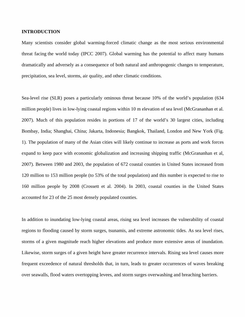
Sea-level rise (SLR) poses a particularly ominous threat because 10% of the world’s population (634

million people) lives in low-lying coastal regions within 10 m elevation of sea level (McGrananhan et al.

2007). Much of this population resides in portions of 17 of the world’s 30 largest cities, including

Bombay, India; Shanghai, China; Jakarta, Indonesia; Bangkok, Thailand, London and New York (Fig.

1). The population of many of the Asian cities will likely continue to increase as ports and work forces

expand to keep pace with economic globalization and increasing shipping traffic (McGrananhan et al,

2007). Between 1980 and 2003, the population of 672 coastal counties in United States increased from

120 million to 153 million people (to 53% of the total population) and this number is expected to rise to

160 million people by 2008 (Crossett et al. 2004). In 2003, coastal counties in the United States

accounted for 23 of the 25 most densely populated counties.

In addition to inundating low-lying coastal areas, rising sea level increases the vulnerability of coastal

regions to flooding caused by storm surges, tsunamis, and extreme astronomic tides. As sea level rises,

storms of a given magnitude reach higher elevations and produce more extensive areas of inundation.

Likewise, storm surges of a given height have greater recurrence intervals. Rising sea level causes more

frequent exceedence of natural thresholds that, in turn, leads to greater occurrences of waves breaking

over seawalls, flood waters overtopping levees, and storm surges overwashing and breaching barriers.

In areas affected by tropical storms, warmer ocean surface temperatures may exacerbate these conditions

by increasing the magnitude of storms (Webster et al. 2005). The recent loss of life and destruction of

property in the northern Gulf of Mexico due to Hurricanes Katrina and Rita in 2005 underscore the

vulnerability of coastal regions to storm surges and flooding. The potential loss of life in low-lying areas

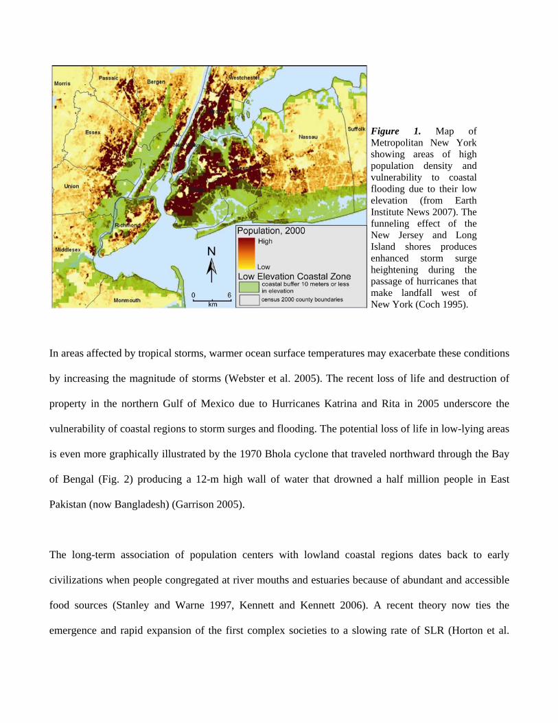
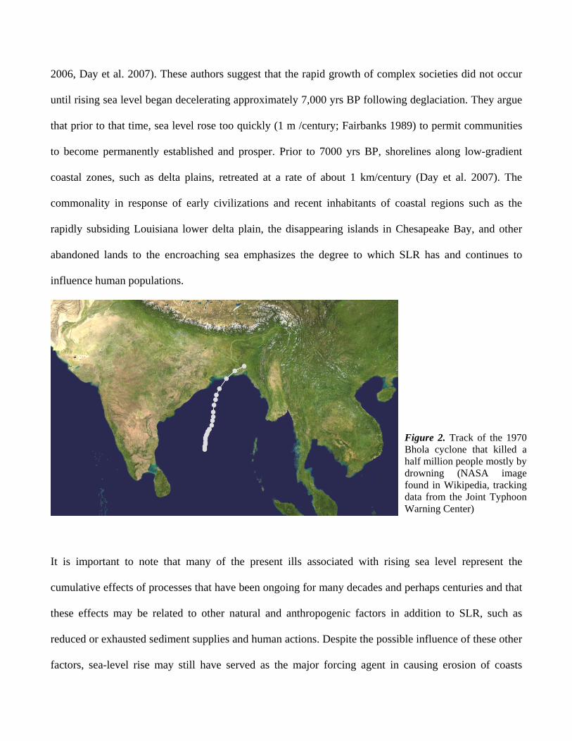
is even more graphically illustrated by the 1970 Bhola cyclone that traveled northward through the Bay

of Bengal (Fig. 2) producing a 12-m high wall of water that drowned a half million people in East

Pakistan (now Bangladesh) (Garrison 2005).

The long-term association of population centers with lowland coastal regions dates back to early

civilizations when people congregated at river mouths and estuaries because of abundant and accessible

food sources (Stanley and Warne 1997, Kennett and Kennett 2006). A recent theory now ties the

emergence and rapid expansion of the first complex societies to a slowing rate of SLR (Horton et al.

Figure 1. Map of Metropolitan New York showing areas of high population density and vulnerability to coastal flooding due to their low elevation (from Earth Institute News 2007). The funneling effect of the New Jersey and Long Island shores produces enhanced storm surge heightening during the passage of hurricanes that make landfall west of New York (Coch 1995).

2006, Day et al. 2007). These authors suggest that the rapid growth of complex societies did not occur

until rising sea level began decelerating approximately 7,000 yrs BP following deglaciation. They argue

that prior to that time, sea level rose too quickly (1 m /century; Fairbanks 1989) to permit communities

to become permanently established and prosper. Prior to 7000 yrs BP, shorelines along low-gradient

coastal zones, such as delta plains, retreated at a rate of about 1 km/century (Day et al. 2007). The

commonality in response of early civilizations and recent inhabitants of coastal regions such as the

rapidly subsiding Louisiana lower delta plain, the disappearing islands in Chesapeake Bay, and other

abandoned lands to the encroaching sea emphasizes the degree to which SLR has and continues to

influence human populations.

It is important to note that many of the present ills associated with rising sea level represent the

cumulative effects of processes that have been ongoing for many decades and perhaps centuries and that

these effects may be related to other natural and anthropogenic factors in addition to SLR, such as

reduced or exhausted sediment supplies and human actions. Despite the possible influence of these other

factors, sea-level rise may still have served as the major forcing agent in causing erosion of coasts

Figure 2. Track of the 1970 Bhola cyclone that killed a half million people mostly by drowning (NASA image found in Wikipedia, tracking data from the Joint Typhoon Warning Center)

worldwide (Leatherman et al. 2000, Pilkey and Cooper 2004). As acknowledged in the recent IPCC

(2007) report, a growing number of tide gage and field studies demonstrate that the rate of SLR began

increasing between the mid-19th and mid-20th centuries, (Nydick et al. 1995, Gehrels 1999, Donnelly

and Bertness 2004, Donnelly 2006) and recent tide gage data suggest that since 1993, the rate of SLR

has increased to 3 mm/yr (Church and White 2006). Thus, many of the impacts of accelerating SLR, can

be generalized as worsening existing long-term conditions. For example, flooding lowlands, beach

erosion, saltwater intrusion, and wetland loss are all processes that have been ongoing along coasts for

centuries and have been widely recognized for many years (Bird 1993, Leatherman 2001).

In addition to increased flooding and greater storm impacts to coastal communities in many low-lying

regions, accelerated SLR will dramatically affect sandy beaches and barrier island coasts. These impacts

go beyond simple inundation caused by rising ocean waters, and involve the permanent or long-term

loss of sand from beaches. The loss results from complex, feedback-dependent processes that operate

within the littoral zone including onshore coastal elements (e.g., the, nearshore, beachface, dunes, tidal

inlets, tidal flats, marshes and lagoons). Sediment budget analyses have shown that nearshore, tidal

deltas, capes, and the inner continental shelf can serve as sediment reservoirs (Komar 1998). Long-term

beach erosion may increase due to accelerated SLR and may eventually lead to the deterioration of

barrier chains such as those along U.S. East and Gulf coasts (Williams et al. 1992, FitzGerald et al.

2007), Friesian Islands in the North Sea, and the Algarve coast in southern Portugal. Barriers protect

highly productive and ecologically sensitive backbarrier wetlands as well as the adjacent mainland coast

from direct storm impacts and erosion. Moreover, barriers support residential communities and a

thriving tourist industry. It is estimated that $3 Trillion are invested in real estate and infrastructure on

the barriers and mainland beaches along the East Coast of the U.S. (Evans 2004). A single 7-km long

barrier in North Carolina, Figure Eight Island, has a tax base of more than $2 Billion (W. Cleary pers.

comm.). In many developing countries tourism is a major part of their economy and the success of this

industry is dependent on the vitality of its beaches.

Determining the socio-economic impacts of sea-level rise on coastal areas comprises one of this

century’s greatest challenges (Titus and Barth 1984, Gornitz 1990, Titus et al. 1991, Nicholls and

Leatherman 1996, Gornitz et al. 2002). This challenge, in turn, depends on accurate determinations of

the effect of accelerated sea-level rise on the natural (physical and ecological) environment. In fact, the

National Assessment of Coastal Vulnerability to Future Sea-Level Rise (USGS 2000) states that

determining the physical response of the coast to SLR constitutes “one of the most important problems

in applied coastal geology today.” Consequently, studies have used various sea-level rise scenarios to

explore the socio-economic, physical and ecological impacts on coasts in the U.S. (e.g., Kana et al.

1984, Park et al. 1989, Weggel et al. 1989, Titus 1990, FEMA 1991, Titus et al. 1991, Yohe et al. 1996,

Wu et al. 2002) and throughout the world (e.g., Paskoff 2004, Walsh et al. 2004, Nicholls and Tol 2006,

Tol et al. 2007).

Rising sea level is affecting coastlines throughout the world; the magnitude and types of impacts are

related to the geologic setting and physical and ecological processes operating in that environment.

Unlike infrequent large-magnitude storms that can change the complexion of coast in a few hours (e.g.

Mississippi coast due to Katrina, http://coastal.er.usgs.gov/hurricanes/ katrina/photo-

comparisons/mainmississippi.html), impacts attributed solely to SLR are usually slow, repetitive, and

cumulative. This paper reviews the state of knowledge concerning the response of coasts to SLR, and

concentrates on coastal plain settings including beaches and barrier chains and associated tidal inlets and

backbarrier wetlands.

SEA LEVEL TRENDS

Although eustatic sea level is presently rising only a few millimeters per year, this condition has

widespread influences on physical and ecological processes on coasts (IPCC 2007). The rate of SLR

determines how quickly areas will be inundated given their slope, the rate at which wetlands, such as

salt marshes, must accrete vertically to maintain their surpratidal and intertidal extent, the rate of erosion

and shoreline recession, and the rate of sand exchange between the beach and the nearshore. Sea level is

a function of the ocean surface, which is a controlled by the: 1. volume of ocean water, 2. volume of the

ocean basins, and 3. distribution of the water, and the land surface, which is affected by crustal

deformation and sediment compaction. Although sea level is influenced by many elements that operate

globally and locally over a wide range of time scales including days to weeks (tides, storms), seasonal

(steric changes, weather), 100 – 104 years (climate, tectonic), and up to millions of years (ocean basin

evolution), the two primary factors dictating the present rate of SLR are thermal expansion due to heat

uptake by ocean surface waters and water input caused by the transfer of water from the land to the

oceans (IPCC 2007).

Earth’s warming since the early 1900’s corresponds well with retreating mountain glaciers, decreasing

snow cover in the Northern Hemisphere, reduction of Arctic ice and with other more subtle proxies,

such as migrational patterns of birds and butterflies, and early growth season of certain plants (IPCC

2007). The record shows that from 1850 to 1915 average global temperatures fluctuated but with no

significant net change. During the past 100 years temperatures have risen by 0.74°C with most of that

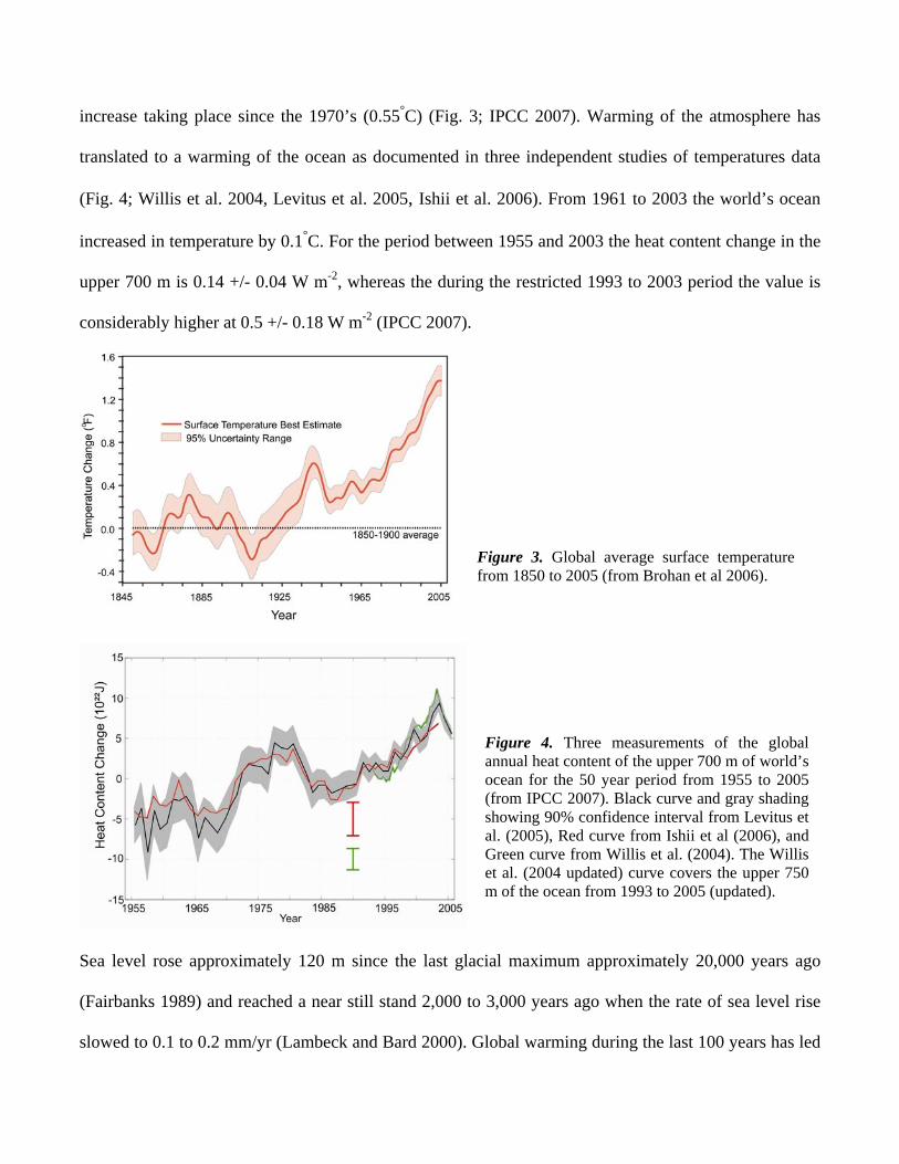
increase taking place since the 1970’s (0.55°C) (Fig. 3; IPCC 2007). Warming of the atmosphere has

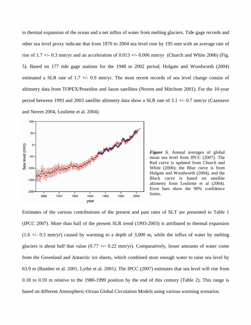
translated to a warming of the ocean as documented in three independent studies of temperatures data

(Fig. 4; Willis et al. 2004, Levitus et al. 2005, Ishii et al. 2006). From 1961 to 2003 the world’s ocean

increased in temperature by 0.1°C. For the period between 1955 and 2003 the heat content change in the

upper 700 m is 0.14 +/- 0.04 W m-2, whereas the during the restricted 1993 to 2003 period the value is

considerably higher at 0.5 +/- 0.18 W m-2 (IPCC 2007).

Sea level rose approximately 120 m since the last glacial maximum approximately 20,000 years ago

(Fairbanks 1989) and reached a near still stand 2,000 to 3,000 years ago when the rate of sea level rise

slowed to 0.1 to 0.2 mm/yr (Lambeck and Bard 2000). Global warming during the last 100 years has led

Figure 3. Global average surface temperature from 1850 to 2005 (from Brohan et al 2006).

Figure 4. Three measurements of the global annual heat content of the upper 700 m of world’s ocean for the 50 year period from 1955 to 2005 (from IPCC 2007). Black curve and gray shading showing 90% confidence interval from Levitus et al. (2005), Red curve from Ishii et al (2006), and Green curve from Willis et al. (2004). The Willis et al. (2004 updated) curve covers the upper 750 m of the ocean from 1993 to 2005 (updated).

to thermal expansion of the ocean and a net influx of water from melting glaciers. Tide gage records and

other sea level proxy indicate that from 1870 to 2004 sea level rose by 195 mm with an average rate of

rise of 1.7 +/- 0.3 mm/yr and an acceleration of 0.013 +/- 0.006 mm/yr (Church and White 2006) (Fig.

5). Based on 177 tide gage stations for the 1948 to 2002 period, Holgate and Woodworth (2004)

estimated a SLR rate of 1.7 +/- 0.9 mm/yr. The most recent records of sea level change consist of

altimetry data from TOPEX/Poseidon and Jason satellites (Nerem and Mitchum 2001). For the 10-year

period between 1993 and 2003 satellite altimetry data show a SLR rate of 3.1 +/- 0.7 mm/yr (Cazenave

and Nerem 2004, Leuliette et al. 2004).

Estimates of the various contributions of the present and past rates of SLT are presented in Table 1

(IPCC 2007). More than half of the present SLR trend (1993-2003) is attributed to thermal expansion

(1.6 +/- 0.5 mm/yr) caused by warming to a depth of 3,000 m, while the influx of water by melting

glaciers is about half that value (0.77 +/- 0.22 mm/yr). Comparatively, lesser amounts of water come

from the Greenland and Antarctic ice sheets, which combined store enough water to raise sea level by

63.9 m (Bamber et al. 2001, Lythe et al. 2001). The IPCC (2007) estimates that sea level will rise from

0.18 to 0.59 m relative to the 1980-1999 position by the end of this century (Table 2). This range is

based on different Atmospheric-Ocean Global Circulation Models using various warming scenarios.

Figure 5. Annual averages of global mean sea level from IPCC (2007). The Red curve is updated from Church and White (2006); the Blue curve is from Holgate and Woodworth (2004), and the Black curve is based on satellite altimetry from Leuliette et al (2004). Error bars show the 90% confidence limits.

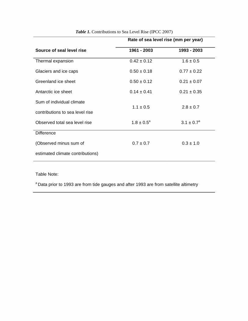
Table 1. Contributions to Sea Level Rise (IPCC 2007)

Rate of sea level rise (mm per year)

Source of seal level rise 1961 - 2003 1993 - 2003

Thermal expansion 0.42 ± 0.12 1.6 ± 0.5

Glaciers and ice caps 0.50 ± 0.18 0.77 ± 0.22

Greenland ice sheet 0.50 ± 0.12 0.21 ± 0.07

Antarctic ice sheet 0.14 ± 0.41 0.21 ± 0.35

Sum of individual climate

contributions to sea level rise 1.1 ± 0.5 2.8 ± 0.7

Observed total sea level rise 1.8 ± 0.5a 3.1 ± 0.7a

Difference

(Observed minus sum of

estimated climate contributions)

0.7 ± 0.7 0.3 ± 1.0

Table Note:

a Data prior to 1993 are from tide gauges and after 1993 are from satellite altimetry

Table 2. Projected trends of SLR based on different warming scenarios (IPCC 2007).

Temperature Change

(oC at 2090-2099 relative to

1980-1999)a

Sea Level Rise

(m at 2090-2099 relative to 1980-

1999)

Case Best

Estimate

Likely

Range

Model-based range excluding

future rapid dynamical changes

in ice flow

Constant Year 2000

concentrations b 0.6 0.3 - 0.9 NA

B1 scenario 1.8 1.1 - 2.9 0.18 - 0.38

A1T scenario 2.4 1.4 - 3.8 0.20 - 0.45

B2 scenario 2.4 1.4 - 3.8 0.20 - 0.43

A1B scenario 2.8 1.7 - 4.4 0.21 - 0.48

A2 scenario 3.4 2.0 - 5.4 0.23 - 0.51

A1F1 scenario 4.0 2.4 - 6.4 0.26 - 0.59

Notes: a These estimates are assessed from a hierarchy of models that encompass a simple climate model, several Earth Models of Intermediate Complexity (EMICs) and a large number of Atmosphere-Ocean Global Circulation Models (AOGCMs). b Year 2000 constant composition is derived from AOGCMs only.

ISLAND AND LOWLAND INUNDATION

One dramatic and immediate effect of SLR is the inundation of low-lying coastal areas around the world

(Bird 1993). In addition to increased coastal erosion caused by SLR, flooding of deltaic regions,

saltwater incursion into coastal urban centers, and disruption of transportation are of great concern in

many countries (Leatherman 1997, Titus 2002, Fig. 6). In their compilation of the countries in the low-

elevation coastal zones (LECZ), McGranahan et al. (2006) report that one in ten people live in coastal

zones less than 10 m in elevation. China has the largest number of people (127 million or 10% of the

total population), whereas in a number of coastal and insular nations with populations exceeding

100,000 people, more than 50% of people live within the LECZ (McGranahan et al. 2006).

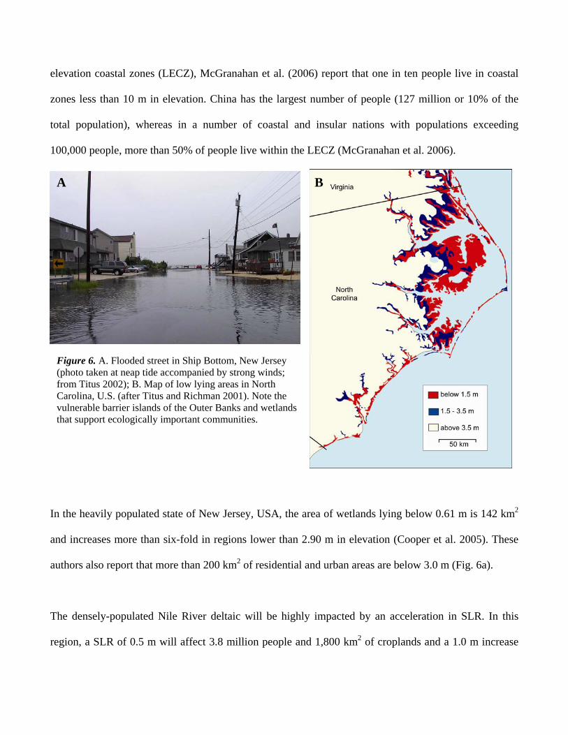
In the heavily populated state of New Jersey, USA, the area of wetlands lying below 0.61 m is 142 km2

and increases more than six-fold in regions lower than 2.90 m in elevation (Cooper et al. 2005). These

authors also report that more than 200 km2 of residential and urban areas are below 3.0 m (Fig. 6a).

The densely-populated Nile River deltaic will be highly impacted by an acceleration in SLR. In this

region, a SLR of 0.5 m will affect 3.8 million people and 1,800 km2 of croplands and a 1.0 m increase

B

Figure 6. A. Flooded street in Ship Bottom, New Jersey (photo taken at neap tide accompanied by strong winds; from Titus 2002); B. Map of low lying areas in North Carolina, U.S. (after Titus and Richman 2001). Note the vulnerable barrier islands of the Outer Banks and wetlands that support ecologically important communities.

A

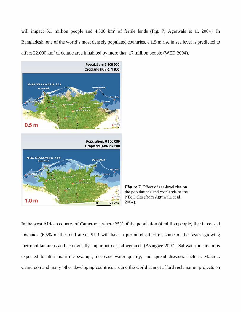
will impact 6.1 million people and 4,500 km2 of fertile lands (Fig. 7; Agrawala et al. 2004). In

Bangladesh, one of the world’s most densely populated countries, a 1.5 m rise in sea level is predicted to

affect 22,000 km2 of deltaic area inhabited by more than 17 million people (WED 2004).

In the west African country of Cameroon, where 25% of the population (4 million people) live in coastal

lowlands (6.5% of the total area), SLR will have a profound effect on some of the fastest-growing

metropolitan areas and ecologically important coastal wetlands (Asangwe 2007). Saltwater incursion is

expected to alter maritime swamps, decrease water quality, and spread diseases such as Malaria.

Cameroon and many other developing countries around the world cannot afford reclamation projects on

0 50 km

Figure 7. Effect of sea-level rise on the populations and croplands of the Nile Delta (from Agrawala et al. 2004).

a scale similar to those in the Netherlands or the Gulf of Mexico. As a consequence, retreat from LECZ

to the hinterlands may be the only option for many coastal communities.

The effect of sea-level rise on small islands and archipelagos has received increased attention due to

vulnerability of their coastal resources and populations to SLR-related coastal flooding (Roy and

Connell 1991, Leatherman 1997, Smithers and Woodroffe 2000, 2001, Dickinson 2004). Whereas some

island nations have coped with SLR and are presently experiencing slightly falling sea level (e.g.,

Maldives, Mörner et al. 2004; but contended by Woodworth 2005), most of them are affected by global

sea-level rise. Because most economic activities on South Pacific islands are concentrated in the coastal

zone, including the capitals of many island states (Fiji, Western Samoa, Tonga, etc.), coastal inundation

is already driving the patterns of re-location for many residents (Nunn and Mimura 1997). In a recent

comprehensive study of Pacific atolls, Dickinson (2004) concludes that SLR may cause overtopping and

submergence of relict mid-Holocene paleo-reef flats, which would drastically increase wave erosion.

This process is an example of the adverse consequences of outer-reef inundation, which would precede

the actual flooding of subaerial parts of the islands and atolls.

In addition to inundation, SLR will cause saltwater intrusion into coastal aquifers, particularly in regions

of high groundwater withdrawal. For the populations of small islands, reduction or disappearance of

potable water may be the greatest impact on their survival, rivaling in importance both coastal erosion

and lowland flooding. Entire island nations are already being affected by saltwater intrusion (Tuvalu,

Marshall Islands, etc; Roy and Connell 1991, Nunn and Mimura 1997) and this hazard should be

considered together with surface flooding associated with rising sea level.

SHORELINE RESPONSE TO SEA LEVEL RISE

Introduction

The various ways that beaches respond to changes in sea level complicate assessments of the impact of

sea-level rise on natural systems. Additionally, as discussed in more detail below, our perspective of an

observed response, and/or our interpretation of a measured response will change as a function of the

time scales over which we view or measure them. For example, using the temporal reference frame of

classical geomorphology (Schumm and Lichty 1965), barrier islands can migrate landward for tens to

hundreds of kilometers over cyclic time scales (Cowell and Thom 1994). At this time scale, often

spanning 103 - 104 years, rising sea levels cause the shoreline to move landward during inundation of a

tectonically or isostatically stable or subsiding terrestrial land surface (Kana et al. 1984) if the sediment

supply rate cannot keep pace with the sea-level rise rate (Curray 1964). Geologic evidence shows that

during the Holocene transgression, coastal barriers, bays, marshes, and wetlands have all experienced

dramatic changes that included the in-place drowning, overstepping, and continuous rolling-over. On

the other end of the temporal spectrum, the daily physical forces associated with sea-level rise (over

steady time periods, 100 years) do not appear to contribute to the net coastal sediment transport regime.

During graded time scales (101 – 102 years), processes other than sea-level rise, such as El Niño, storm

surges, or seasonal wave climate variations, control beach morphological responses (e.g., Storlazzi and

Griggs 2000). Moreover, the global effects of sea-level rise on coasts will vary spatially (Gornitz 1991).

As a consequence, some coastal scientists have advocated analyzing and predicting coastal changes on a

more local scale (Pilkey and Davis 1987, Fenster and Dolan 1993, Pilkey et al. 1993, Cooper and Pilkey

2004).

The need to predict and manage the potential impact of sea-level rise on coasts necessitates accurate

models. Statistical modeling usually involves projecting historical shoreline changes into the future

(e.g., NRC 1990, Fenster et al. 1993, Douglas et al. 1998). The NRC (1990) refers to this approach as

“Historical Trend Analysis.” This response-based approach uses time as a surrogate for processes and

coastal response is measured by trend delineation of historical shoreline positions (Dolan et al. 1991).

Despite this limitation, Leatherman (1984) suggested using historical trends, coupled with an estimate of

sea-level rise, to develop a rule of thumb capable of predicting shoreline recession rates. This approach

assumes that sea-level rise entirely controls shoreline trends. Leatherman et al. (2000) and Zhang et al.

(2004) expanded the concept that a direct relationship exists between sea-level rise and shoreline

recession over centennial to decadal time scales only to have these ideas meet resistance in the coastal

community (Pilkey et al. 2000, Sallenger et al. 2000, Cooper and Pilkey 2004). Conceptual, empirical,

and mathematical models are also used extensively to predict the impact of sea-level rise on coasts.

While these models attempt to link responses with the processes responsible for those changes, each

have limitations. In general, the coastal sciences do not have a holistic model available to make those

links reliably in multiple settings (e.g., Cooper and Pilkey 2004, Cowell et al. 2006, Stolper et al. 2005,

Fenster 2006). Given this constraint, we examine several of the most widely used models to link sea-

level changes to coastal responses in general and shoreline migration in particular and the fundamental

concepts upon which these models rely.

The Equilibrium Profile: A Central Concept

The equilibrium profile has remained a central component of models that predict shoreline retreat based

on sea-level rise since the inception of the Bruun (1954, 1962) Rule as well as one of the central themes

in coastal geology and sedimentation (Swift and Palmer 1978). Fenneman (1902) and Johnson (1919)

first speculated that shore profiles along unconsolidated coasts develop a constant, concave upwards

shape following adjustments of current, slope and sediment load. The equilibrium profile is a time-

averaged response to variations in energy and sediment supply and consists of a shorter and steeper

limb near the shoreline and longer, flatter limb farther offshore (e.g., Moore and Curray 1964, Dean

1991). In theory, fluctuations to the profile produced by the wave climate (i.e., seasonal variations or

storms) and currents maintain the equilibrium profile at a given water-level position, but do not alter its

long-term average form. Additionally, coastal scientists have distinguished between an “ideal” profile

and a “dynamic” equilibrium profile (NRC 1987, Pilkey et al. 1993) where the former represents a

“true” geometric equilibrium profile shape, and the latter undergoes time-dependent profile adjustments

about a long-term average shape. In any case, more than a century of research has shown that coastal

systems tend toward equilibrium configurations with defined geometries despite the inherent variability

of nearshore processes (Fagherazzi et al. 2003).

The equilibrium profile concept implies that cross-shore profiles maintain a concave up, exponential

shape in which the limb nearest the shoreline is shorter and steeper (statistically time-averaged response

to variations in energy and sediment supply, e.g., Moore and Curray 1964). Attempts to confirm the

existence of or to quantify the shape of the equilibrium profile have come from laboratory experiments

(Eagleson et al. 1963, Schwartz 1965, Vellinga 1982, Kriebel 1986), empirical studies (see summary in

Woodroffe 2002), and modeling efforts (Cowell et al. 1995, Niedoroda et al. 1995, Stive and de Vriend,

1995, Stolper et al. 2005, Moore et al. 2006). Each approach has its advantages and disadvantages. For

example, laboratory confirmation must contend with scale effects and limitations of monochromatic

waves (Cooper and Pilkey 2004). Empirical studies, though often quantitative in nature, provide a

descriptive method devoid of a process- or physics-based approach (Dean 1991, Pilkey et al. 1993).

Mathematical models may have shortcomings due to their assumptions and inability to account for

uncertainty or stochastic processes (Pilkey 1994). Nevertheless, some of these approaches have

independently and collectively revealed equilibrium profiles may exist at relatively broad spatial and

long temporal scales or at site-specific reaches (Fenster and Miller 2001, Pilkey et al. 1993).

Curve fitting techniques through bathymetric data have provided an empirical means to examine cross-

shore profiles. For example, using data from the Denmark and southern California coasts, Bruun (1954)

described the geometry of the equilibrium profile with a power function equation that relates profile

shape at a water depth, h, to distance offshore (x) and a scale factor, A, constrained primarily by

sediment characteristics:

h(x) = Ax2/3. (1)

Dean (1977) verified this relationship using a profile data set from Hayden et al. (1975) and

corroborated the exponent value of 2/3 originally provided by Bruun (1962). Moreover, Dean (1977)

found that the shape factor, A, depends primarily on sediment characteristics and speculated that the

monotonic profile form is consistent with uniform wave energy dissipation per unit volume of the water

column within the surf zone. However, Wang and Davis (1998) empirically showed that equation (1)

describes the inner surf zone better than the landward slope of breakpoint-bar and nearshore zone.

Additional studies involving empirical orthogonal functions (EOF) have purported to confirm the

existence of a(n) (quasi-) equilibrium profile (Hayden et al. 1975, Weishar and Wood 1983, Fenster and

Miller, 2001). These studies have uniformly shown that, because the first one or two eigenvectors

capture most of the total variance, a regional control (i.e., sea-level) on profile shape must exist. Dean

(1977) corroborated the exponent value of 2/3 originally provided by Bruun (1962) and found that the

shape factor, A, depends primarily on sediment characteristics and speculated that the monotonic profile

form is consistent with uniform wave energy dissipation per unit volume of the water column within the

surf zone. However, in a cross-shore sense, Wang and Davis (1998) showed that equation (1) describes

the inner surf zone better than the landward slope of breakpoint-bar and nearshore zone.

After reviewing the works of those that attempted to characterize equilibrium beach profiles (Bruun

1954, Eagleson et al. 1963, Swart 1974, Suh and Dalrymple 1988) and to develop the scale parameters

of equation (1) (Noda 1972, Winant et al. 1975, Dalrymple and Thompson 1976, Hughes 1983), Dean

(1991) presented a modified equilibrium beach profile that takes into account the unrealistic

consequence of equation (1), namely the infinite slope at the shoreline. In particular, Dean (1991) added

two terms to account for the gravitational (as a destabilizing force) and turbulent effects. Dean (1991)

goes on to make a case for using equilibrium beach profile concepts for application to various coastal

engineering projects, such as sea-wall and nourishment design, because non-equilibrium conditions can

be considered as well. In addition, Moutzouris (1991) and Work and Dean (1991) modified equation (1)

to improve upper beach profile adjustment predictions and to account for variable cross-shore sediment

grains sizes. Later, Bodge (1992), and Komar and McDougal (1994), developed exponential models

that also use empirical coefficients to improve the mathematical representation of the equilibrium profile

in general and slope predictions near the shore in particular.

Within the active zone (between the landward and seaward boundaries) of sediment transport a variety

of processes produce the shoreface slope. These processes operate over multiple time scales. Swift et al.

(1985) concluded that the relative sea-level rise rate, the sediment supply, and rate of fluid power

expenditure control the geometry of the shoreface. Dean (1991) describes sediment transport within the

coastal zone as a competition between boundary layer forces where constructive bottom shear stresses

move sediments landward and destructive stresses that displace sediments seaward. In this sense,

equilibrium profiles exhibit a condition where no cross-shore or longshore sediment transport occurs

because a balance exists between forces causing sediment transport such that the motion of individual

sand grains remains static (USCOE 2002). Pilkey et al. (1993) point out that wave climate is but one

factor that produces the fluid power necessary for sediment transport. Wright et al. (1991) conducted an

extensive field study in the southern Middle Atlantic Bight of the U.S. coast and found that time-

dependent processes – including mean flows, incident waves, long-period waves, and gravity –

contribute to the rates, directions and mechanisms of cross-shore sediment flux. This suite of processes

moves sediment in both a shoreward and seaward direction across the shoreface. In short, because the

forces that initiate and maintain sediment transport operate over varying time scales, determining the

effect of sea-level rise on the shoreline necessitates parsing or identifying individual processes at each

time scale. Thus, one of the greatest problems in the coastal sciences ensues. In fact, the difficulty

involved in relating processes to responses, in part, has hindered development of a physics-based

approach to predicting equilibrium beach profiles (Dean 1991, Cooper et al. 2004), called to question the

concept of shoreface equilibrium in general (Wright et al. 1991), and has spawned debates on the role of

sea-level rise as a causative factor in coastal erosion (Leatherman et al. 2000, Leatherman 2001, Galvin

2000, Pilkey et al. 2000, Sallenger et al. 2000, Zhang et al. 2004).

Over centennial to millennial time scales, some scientists have suggested that cross-shore profiles in

general and the shoreface in particular will shift landward in response to sea-level rise while maintaining

an equilibrium profile, given other potential factors (e.g., sediment supply) remain constant (Swift et al.

1985). This landward shifting profile adjusts dynamically while maintaining its characteristic, concave

upwards shape – the geometry of which is determined by the relative magnitudes of the driving forces

(Swift et al. 1985). Viewed over this time scale, barrier island evolutionary models have two

components: (1) A long-term component (e.g., overwash, and sea level variations) responsible for

barrier evolution and migration and (2) A short-term process component that leads to an equilibrium

profile (Swift et al. 1985, Fagherazzi et al. 2003).

Viewed over decadal to centennial time scales, i.e., those that affect human activities along the coast, an

accepted conceptual model envisions sea-level rise as a factor in profile evolution in that it allows high

energy, short period storm waves to attack (do most of their work on) the beach on the shallowest and

subaerial parts of the profile (NRC 1987). If the profile displayed a planar shape or linear slope, water-

level increases would not result in disequilibrium. However, increases in water levels on non-linear,

exponentially-shaped profiles result in profiles that must recede in order to maintain conservation of

sediment mass (USCOE 2002). In this case, the “allied roles” (NRC 1987) of sea-level rise and wave

activity create beach and nearshore profiles that are out of equilibrium.

Over relatively short-time scales, beaches respond to a variety of factors including the resultant vectors

of constructive and destructive forces, sediment budgets, sediment characteristics, and inherited

shoreface geology (Dean 1991, Fenster and Dolan 1993, Cowell et al. 2005). Thus, over the short term,

the shore responds episodically to a variety of coastal processes and wave climate plays a role in

determining profile shape, but not exclusive to a myriad of other processes (Komar et al. 1991). In fact,

the role of bottom currents (i.e., other processes besides wave orbital interactions with the shoreface)

weakens assumptions used in models that utilize the equilibrium profile concept.

Distinguishing between long- and short-term processes and responses provides a method for correctly

interpreting the impact of sea-level rise and other coastal processes on beach and nearshore responses

(Everts 1985, Clarke and Eliot 1983, Dolan et al. 1991, Fenster et al. 1993). Indeed, Bruun (1988) asks,

“How long a period of time is required to enable us to measure the reaction of the profile to a long-term

rise in sea level?” For example, empirical studies have showed that profile equilibrium is approached

over decadal time spans because of the phase lag between the processes and responses (Hands 1983).

Statistical approaches have identified a minimum of 10-24 years as the amount of time required to

separate noise from a signal (Everts 1985, Dolan et al. 1991, Clarke and Eliot 1983, 1987, Bruun 1988).

The inherent variability of natural systems thus requires examination of coastal processes and responses

on a case-by-case and site-by-site basis (Dean 1987, Pilkey et al. 1993).

The concept of equilibrium profile has not met pervasive acceptance in the coastal sciences. Arguments

to this concept include: (1) differentiating between relict and active continental shelves (Dietz 1963);

(2) the notion that sediment characteristics (e.g., scale factor A in equation [1]), including grain size and

fall velocity, can determine profile shape have been based on the ideas that the assumption is unrealistic

outside the surf zone (Bruun 1988, Pilkey et al. 1993, Theiler et al. 2000, Pilkey and Cooper 2004,

Cooper and Pilkey 2004); (3) determination of the parameters – including grain size – comes from a

non-physics based, empirical approach that has omitted germane results (Pilkey et al. 1993, Theiler et al.

2000, Pilkey and Cooper 2004, Cooper and Pilkey 2004); (4) limitations of mathematical models that

predict shoreline retreat as a function on sea-level rise – e.g., non-sandy antecedent geologic conditions,

cross-shore variations in sediment type, sediment-starved environments, offshore sediment losses

beyond the “active” sediment transport prism or nearshore, tectonically or isostatically active coasts, a

model’s inability to provide the kinematics and/or dynamics required to maintain the equilibrium profile

(Pilkey et al. 1993, Theiler et al. 2000, Pilkey and Cooper 2004); (5) the use of two dimensional models

in a three-dimensional system and the problems associated with system boundaries.

With respect to longshore boundaries (normal to cross-shore transport direction), two-dimensional

models used to predict shoreline change as a function of sea-level rise do not consider longshore

gradients (i.e., longshore boundaries are infinitesimally small, ∂Qs/∂Y = 0 or constant, where Qs is the

sediment transport flux in a longshore direction, and Y is the sediment volume/time entering a control

volume not caused by relative sea-level rise). On the other hand, three dimensional models have

parameters that provide input parameters for longshore sediment transport fluxes and thus, provide a

sediment budget approach to predicting shoreline changes based on sea-level rise (e.g., Everts 1985,

Dubois 1995). Apparently, separate approaches to quantifying either longshore or cross-shore transport

have developed because of the tendency for coasts to have one component dominate over another in any

one location (USCOE 2002). The seaward boundary, aka “closure depth,” is a major factor in the

modeling and interpretation of morphological changes as a function of sea-level rise (e.g., Komar et al.

1991). The closure depth delineates the nearshore or shoreface (landward of closure depth to the

shoreline) and the offshore or ramp (seaward of closure depth). This dynamic “sand fence” typically

occurs between the seaward large-scale circulation environments of the middle and outer shelf and the

landward friction-dominated environment dominated by shoaling waves (Wright et al. 1991) despite the

recognition that marine currents can predominate on the lower shoreface (Swift et al. 1985). Existence

of this boundary requires an assumption that all sediment erosion, transport, and deposition occurs

landward of closure depth. While this assumption holds true within an envelope or range of beach

profile variability (e.g., Hands 1980), the assumption does not appear to hold true in all cases. For

example, Komar et al. (1972) suggest storm waves can suspend and transport sediment capable of

forming oscillatory ripple marks to depths of 100 – 200 m. Coelho and Veloso-Gomes (2004) found

that field measurements could not confirm predicted depth of closure values for the northwest

Portuguese coast primarily because of temporal variability in grain sizes across the profile. However,

Hallermerier (1991) and Berkemeier (1985) provided a procedure for determining closure depth based

on the wave climate and sediment characteristics. However, both the cross-shore and longshore

boundaries move over time. Consequently, boundary locations are tied to the time-scale of interest.

Dean and Maurmeyer (1983) and Everts (1985) point out that changes in beach profiles over time from

one equilibrium state to another do not necessarily occur with a constant profile form (the profile

configuration is not relevant for modeling, only the maintenance of its shape during sea-level changes).

Consequently, even on sandy substrates, progressive changes over time in profile geometry (i.e.,

sequential gradient changes) violate assumptions of equilibrium profile maintenance needed to drive

predictive models (Komar et al. 1991). For example, shoreline change prediction accuracy decreases

and uncertainty increases as profiles become steeper or flatter over time (Everts 1985). However,

Moore and Curray (1964) pointed out that confusion arises when trying to discuss profile of equilibrium

in the context of topography, morphology, or the nature of the bottom sediments. For example, shelves

possessing a sediment veneer overlying a relict morphology can be in equilibrium while the

morphological profile is not (Curray 1960). Finally, a lag time between changing coastal process

conditions and profile responses or make testing theoretical models difficult (Komar et al. 1991).

However, it is important to note that, despite the limitations mentioned above, most two-dimensional

models that predict shoreline changes as a function of sea-level rise are insensitive to the relationships

among model terms and the dynamics involved in creating the profile (Komar et al. 1991) and models

provide an upper limit on shoreline retreat predictions (Dean and Maurmeyer 1983).

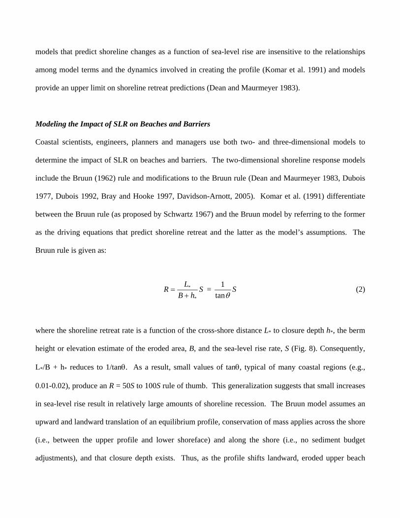
Modeling the Impact of SLR on Beaches and Barriers

Coastal scientists, engineers, planners and managers use both two- and three-dimensional models to

determine the impact of SLR on beaches and barriers. The two-dimensional shoreline response models

include the Bruun (1962) rule and modifications to the Bruun rule (Dean and Maurmeyer 1983, Dubois

1977, Dubois 1992, Bray and Hooke 1997, Davidson-Arnott, 2005). Komar et al. (1991) differentiate

between the Bruun rule (as proposed by Schwartz 1967) and the Bruun model by referring to the former

as the driving equations that predict shoreline retreat and the latter as the model’s assumptions. The

Bruun rule is given as:

ShB

LR

*

*

+= = S

θtan1 (2)

where the shoreline retreat rate is a function of the cross-shore distance L* to closure depth h*, the berm

height or elevation estimate of the eroded area, B, and the sea-level rise rate, S (Fig. 8). Consequently,

L*/B + h* reduces to 1/tanθ. As a result, small values of tanθ, typical of many coastal regions (e.g.,

0.01-0.02), produce an R = 50S to 100S rule of thumb. This generalization suggests that small increases

in sea-level rise result in relatively large amounts of shoreline recession. The Bruun model assumes an

upward and landward translation of an equilibrium profile, conservation of mass applies across the shore

(i.e., between the upper profile and lower shoreface) and along the shore (i.e., no sediment budget

adjustments), and that closure depth exists. Thus, as the profile shifts landward, eroded upper beach

sediment is transported offshore and deposited such that the vertical accretion equals the magnitude of

sea-level rise.

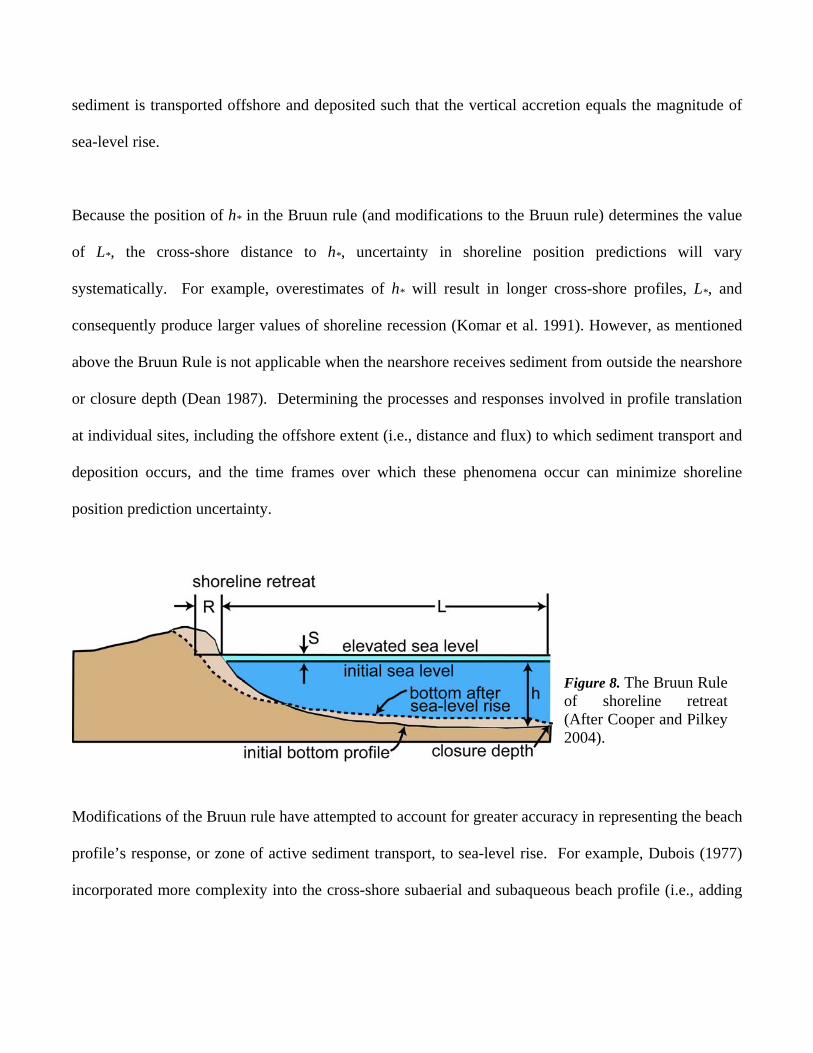
Because the position of h* in the Bruun rule (and modifications to the Bruun rule) determines the value

of L*, the cross-shore distance to h*, uncertainty in shoreline position predictions will vary

systematically. For example, overestimates of h* will result in longer cross-shore profiles, L*, and

consequently produce larger values of shoreline recession (Komar et al. 1991). However, as mentioned

above the Bruun Rule is not applicable when the nearshore receives sediment from outside the nearshore

or closure depth (Dean 1987). Determining the processes and responses involved in profile translation

at individual sites, including the offshore extent (i.e., distance and flux) to which sediment transport and

deposition occurs, and the time frames over which these phenomena occur can minimize shoreline

position prediction uncertainty.

Modifications of the Bruun rule have attempted to account for greater accuracy in representing the beach

profile’s response, or zone of active sediment transport, to sea-level rise. For example, Dubois (1977)

incorporated more complexity into the cross-shore subaerial and subaqueous beach profile (i.e., adding

Figure 8. The Bruun Rule of shoreline retreat (After Cooper and Pilkey 2004).

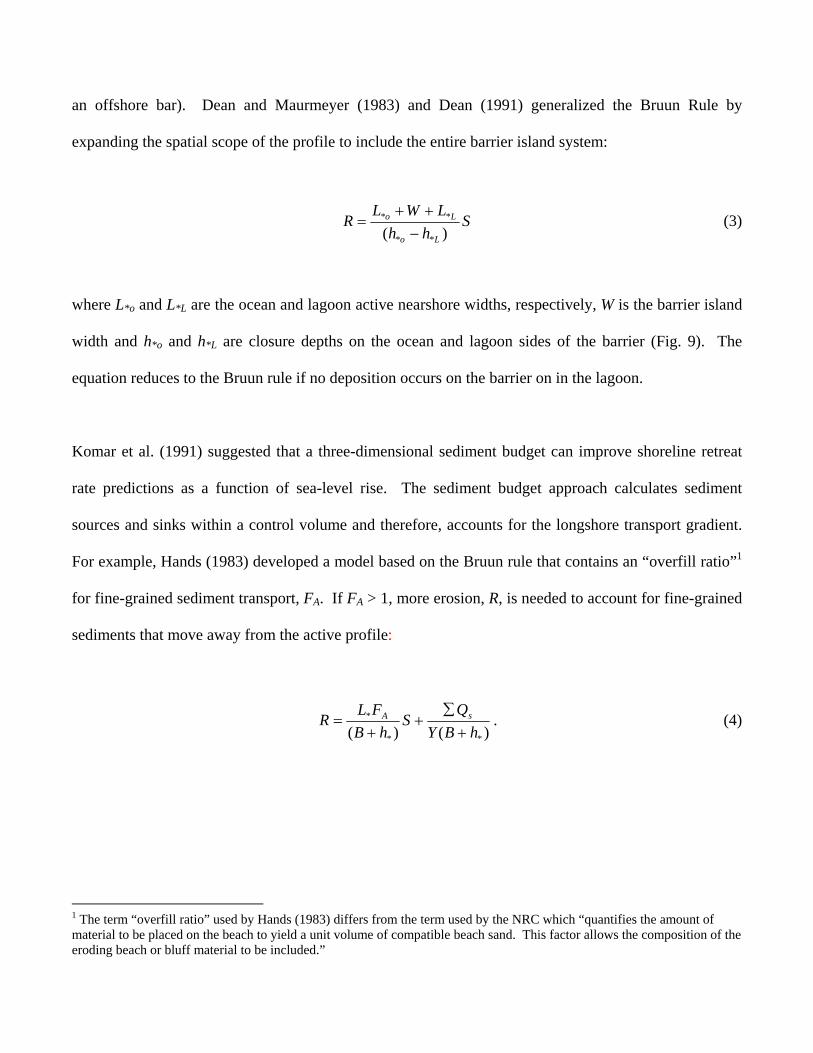
an offshore bar). Dean and Maurmeyer (1983) and Dean (1991) generalized the Bruun Rule by

expanding the spatial scope of the profile to include the entire barrier island system:

Shh

LWLR

Lo

Lo

)( **

**

−++

= (3)

where L*o and L*L are the ocean and lagoon active nearshore widths, respectively, W is the barrier island

width and h*o and h*L are closure depths on the ocean and lagoon sides of the barrier (Fig. 9). The

equation reduces to the Bruun rule if no deposition occurs on the barrier on in the lagoon.

Komar et al. (1991) suggested that a three-dimensional sediment budget can improve shoreline retreat

rate predictions as a function of sea-level rise. The sediment budget approach calculates sediment

sources and sinks within a control volume and therefore, accounts for the longshore transport gradient.

For example, Hands (1983) developed a model based on the Bruun rule that contains an “overfill ratio”1

for fine-grained sediment transport, FA. If FA > 1, more erosion, R, is needed to account for fine-grained

sediments that move away from the active profile:

)()( **

*

hBYQ

ShB

FLR sA

+∑

++

= . (4)

1 The term “overfill ratio” used by Hands (1983) differs from the term used by the NRC which “quantifies the amount of material to be placed on the beach to yield a unit volume of compatible beach sand. This factor allows the composition of the eroding beach or bluff material to be included.”

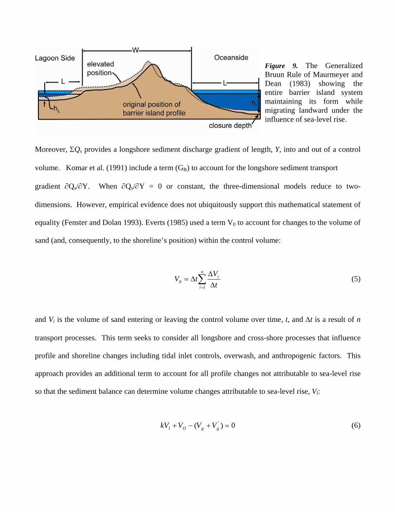
Moreover, ΣQs provides a longshore sediment discharge gradient of length, Y, into and out of a control

volume. Komar et al. (1991) include a term (GB) to account for the longshore sediment transport

gradient ∂Qs/∂Y. When ∂Qs/∂Y = 0 or constant, the three-dimensional models reduce to two-

dimensions. However, empirical evidence does not ubiquitously support this mathematical statement of

equality (Fenster and Dolan 1993). Everts (1985) used a term V0 to account for changes to the volume of

sand (and, consequently, to the shoreline’s position) within the control volume:

∑= ΔΔ

Δ=n

i

i

tV

tV1

0 (5)

and Vi is the volume of sand entering or leaving the control volume over time, t, and Δt is a result of n

transport processes. This term seeks to consider all longshore and cross-shore processes that influence

profile and shoreline changes including tidal inlet controls, overwash, and anthropogenic factors. This

approach provides an additional term to account for all profile changes not attributable to sea-level rise

so that the sediment balance can determine volume changes attributable to sea-level rise, Vl:

0)( ' =+−+ ggOl VVVkV (6)

Figure 9. The Generalized Bruun Rule of Maurmeyer and Dean (1983) showing the entire barrier island system maintaining its form while migrating landward under the influence of sea-level rise.

where k is the volume of sand-sized or larger-grained sediment in Vl, and Vg and 'gV are the volumes of

sand-sized material on the backbarrier and shoreface, respectively and are derived from Vl. Despite this

modeling approach the NRC (1987) claims that the lack of reliable data, such as annualized values of

longshore transport volumes, tidal inlet affects, overwash, and offshore volumetric losses/gains can

constrain these approaches.

Bruun (1988) presents a discussion of the two- and three-dimensional uses of the Bruun rule. Komar et

al. (1991) provide a more comprehensive evaluation of the two and three-dimensional beach response to

sea-level rise models that existed prior to 1991. Cooper and Pilkey (2004) provide a comprehensive

review of the Bruun Rule. Davidson-Arnott (2005) present the most recent revision of shoreline retreat

models as a function of sea-level rise.

Morphological-behavior Models (Large-scale Coastal Behavior, LSCB Models)

Beginning in the 1990s, a suite of quantitative large-scale coastal behavior (LSCB) models developed

which aimed to simulate the large-scale morphologic and stratigraphic evolution of coasts that results

from changes in sea-level and sediment volume (Cowell et al. 1995, Niedoroda et al. 1995, Stive and de

Vriend 1995, Stolper et al. 2005, Moore et al. 2006, Moore et al. 2007). Similar to the shoreline

response models that use time as a surrogate for processes, the LSCB models utilize geometric cross-

shore profile parameters as a proxy for processes. Specifically, these conservation of mass-shoreface

translation models are governed by a sea-level rise scenario and use a set of parameters that rely on the

equilibrium slope concept, an initial volume of (shoreface, barrier, and estuary) sediment, a substrate

slope, and a substrate sand content. The original Shoreface Translation Model (STM; Cowell et al.

1992, 1995) sought to deliver numerical solutions for profile kinematics while simulating the effects of

geological inheritance – one of the criticisms of the Bruun Rule – as well as storm processes, sea-level

changes and variable sediment budgets. The goal of the model is to minimize the number of model

parameters that govern large-scale coastal evolution (to reduce uncertainty), but to maximize the

model’s potential to capture system complexity. Spatially, the models can provide site-specific analysis

at one profile, large-scale analysis because the model aggregates the spatial variability of an entire

coastal cell into one shore-normal profile (that presumably captures both boundary conditions and

driving forces) and a quasi-3D application.

Stolper et al. (2005) sought to improve on the prototype STM of Cowell et al. (1992, 1995) with the

GEOMBEST (Geomorphic Model of Barrier, Estuarine, and Shoreface Translations) model. This model

defines the substrate by stratigraphic and sedimentologic properties such as erodibility (graded

resistance to the erosion potential) and composition instead of requiring an unlimited unconsolidated

sediment supply. This quality enables the model to assess the geological framework when simulating

morphological evolution and shoreline migration. Unlike models that depend on equilibrium profiles (as

explained above), GEOMBEST can account for the disequilibrium found on some shorefaces and, in

fact, is driven by the disequilibrium produced sea-level changes and the vertical displacement of the

profile, for example (e.g., Pilkey et al. 1993, Wright 1995, Thieler et al. 1995, 2000). Validation of

these models, and a simulated evolutionary history of a particular setting for a given sea-level trend,

comes through inverse modeling whereby a known stratigraphy and residual surface serve as the end

member toward which trial and error simulation experiments move.

Moore et al. (2006, 2007) used GEOMBEST to determine sea-level rise was the single greatest

causative factor in controlling the evolutionary history of the Outer Banks near Cape Hatteras followed

by changes in the sediment budget. Additionally, Moore et al. (2007) used GEOMBEST to predict

future impacts of various sea-level rise scenarios for AD2100 on LSCB. Model runs using low, middle,

and high IPCC (2001) sea-level rise estimates showed that a 0.9 m increase in sea-level will increase

erosion rates of up to 2.5 times the present-day rates found in erosion hot spots (Morton et al. 2005).

However, Moore et al. (2007) conjectured that the barrier could remain in tact given that rapid migration

currently exists on other barriers (Morton et al. 2004, Penland et al. 2005). However, simulation runs

using the 1.4 m – 1.9 m rise in sea level by AD2100 show that “threshold collapse” and subsequent

drowning could occur along the Outer Banks similar to the modern day analog of Louisiana’s Isle

Dernieres.

WETLANDS

Background

Coastal wetlands have increasingly been recognized as a unique and vulnerable habitat, a transitional

zone between tidal flats and uplands exposed to extremes of temperature, salinity and inundation by tidal

waters. Salt marshes cover extensive areas of estuarine and deltaic environments in mid to high

latitudes. They are among the most productive ecosystems on Earth (Nixon 1980, Childers et al. 2002)

and provide benefits to coastal communities by filtering surface waters, buffering storm energies and

storing flood waters (Mitsch and Gosselink 2000, Kennish 2001). Salt marshes today are threatened

worldwide by accelerating sea-level rise (SLR) (Church and White 2006, Morris et al. 2002, Reed

2002).

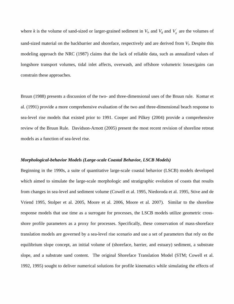
Tidal marshes are maintained through delicate balances between: accretion and subsidence;

bioproductivity and decomposition; erosion and vegetative stabilization; and tidal prism and drainage

efficiency (Cahoon et al. 1995, French 2006, Morris et al. 2002). These processes are in turn controlled

by complex inter-related feedbacks with physical parameters including climate, sea level, and regional

tectonics (Fig. 10).

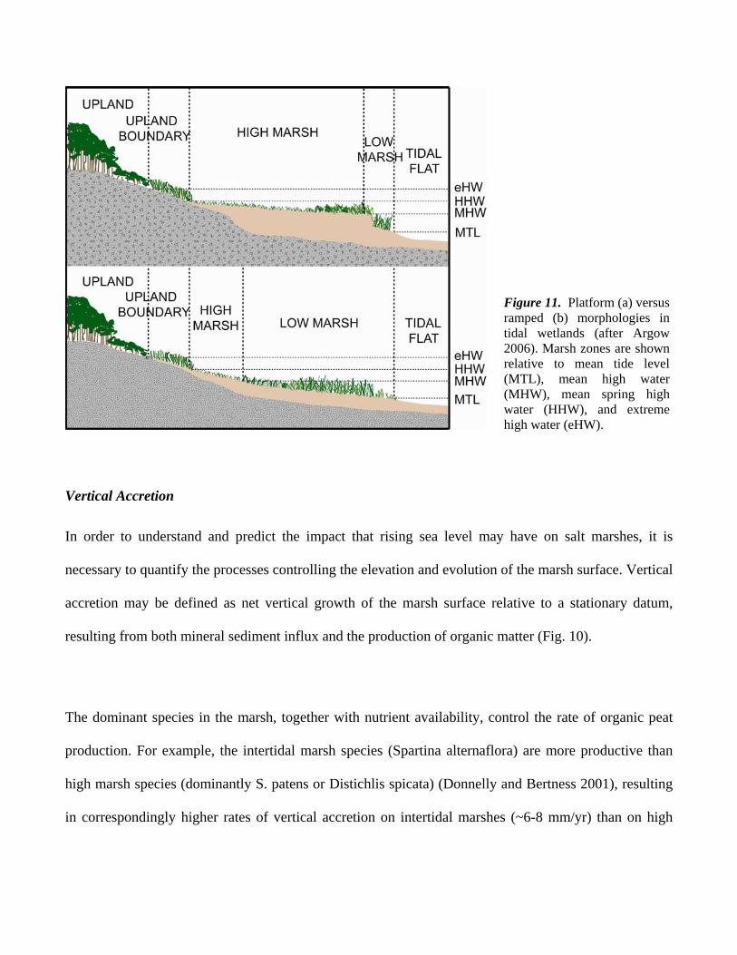
Salt marsh morphology is both a function of, and a control on, these parameters. There are two major

salt marsh morphologies: ramped or platform (Fig. 11), corresponding to a predominance of either tidal

sedimentation or bioproductivity, respectively, as the key driver of accretion (Allen 2000, French 2006).

Marshes dominated by supratidal, or high marsh (Fig. 11a) exhibit a platform-like morphology.

Supratidal marsh peat is more highly organic than intertidal marsh peat, reflecting lower influx of

inorganic sedimentation due to reduced frequency, duration and depth of tidal inundation (Argow 2006).

Intertidal marshes, dominated by low marsh, may exhibit ramped (Fig. 11b), platform, or mixed

morphology, depending on the relative influx of inorganic sedimentation, tidal range, and wave climate

(Allen 2000, Morris et al. 2002).

Figure 10. Conceptual model of the major factors affecting marsh elevation (after Argow 2006)

Vertical Accretion

In order to understand and predict the impact that rising sea level may have on salt marshes, it is

necessary to quantify the processes controlling the elevation and evolution of the marsh surface. Vertical

accretion may be defined as net vertical growth of the marsh surface relative to a stationary datum,

resulting from both mineral sediment influx and the production of organic matter (Fig. 10).

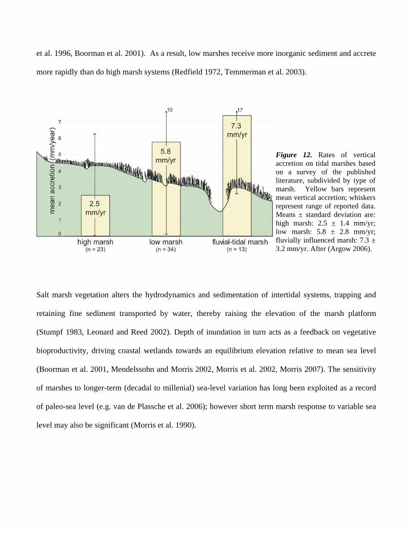
The dominant species in the marsh, together with nutrient availability, control the rate of organic peat

production. For example, the intertidal marsh species (Spartina alternaflora) are more productive than

high marsh species (dominantly S. patens or Distichlis spicata) (Donnelly and Bertness 2001), resulting

in correspondingly higher rates of vertical accretion on intertidal marshes (~6-8 mm/yr) than on high

Figure 11. Platform (a) versus ramped (b) morphologies in tidal wetlands (after Argow 2006). Marsh zones are shown relative to mean tide level (MTL), mean high water (MHW), mean spring high water (HHW), and extreme high water (eHW).

marshes (~2-3 mm/yr) (FitzGerald et al. 2006). The highest rates of marsh vertical accretion are found

in fluvially-dominated systems (Fig. 12).

Tidal sedimentation is a key parameter in this complex system. The fundamental parameters governing

inorganic suspended sediment transport and deposition on salt marshes include tidal range and

inundation depth, vegetation density, and rates of particle settling. There is extensive treatment in the

literature of tidal marsh sedimentation ( Day et al. 1999, Allen 2000, French, 2006). Inorganic sediment

influx on short time scales is controlled by tidal currents and the suspended sediment load, as sediment

is deposited during high slack water. Deposition is aided by the drag created by vegtation ( Nepf et al.

1997, Leonard and Reed 2002). Over longer time scales, episodic storms deposit coarser sediments in

the marsh, rapidly elevating the marsh surface (Donnelly et al. 2004, Cahoon 2006). Storms and other

episodic events may deliver sediment volumes in a single event that are orders of magnitude greater than

single-tide sedimentation rates (Stumpf 1983, Leonard and Reed 2002) and may even impact marshes

where the dominant supply of inorganic sediments is fluvial, e.g the Mississippi delta region (Reed

2002, Cahoon 2006). In northern marshes, ice-rafted sediment is deposited during winter spring tides

and storms (Redfield 1972, van Proosdij et al. 2006).

Within the marsh, spatial variation in tidal sedimentation rates has been attributed to two main physical

parameters: 1. marsh surface elevation; and 2. distance from tidal creeks and the leading marsh edge,

with respect to vegetative biomass. Total suspended sediment increases linearly with depth of tidal

inundation, giving rise to an exponential relationship between inundation time and sedimentation rate

(Leonard and Reed 2002, Paquette et al. 2004). Accordingly, sedimentation rates decrease with

increasing marsh surface elevation (Stumpf 1983, Stoddart et al. 1989, Hutchinson et al. 1995, Callaway

et al. 1996, Boorman et al. 2001). As a result, low marshes receive more inorganic sediment and accrete

more rapidly than do high marsh systems (Redfield 1972, Temmerman et al. 2003).

Salt marsh vegetation alters the hydrodynamics and sedimentation of intertidal systems, trapping and

retaining fine sediment transported by water, thereby raising the elevation of the marsh platform

(Stumpf 1983, Leonard and Reed 2002). Depth of inundation in turn acts as a feedback on vegetative

bioproductivity, driving coastal wetlands towards an equilibrium elevation relative to mean sea level

(Boorman et al. 2001, Mendelssohn and Morris 2002, Morris et al. 2002, Morris 2007). The sensitivity

of marshes to longer-term (decadal to millenial) sea-level variation has long been exploited as a record

of paleo-sea level (e.g. van de Plassche et al. 2006); however short term marsh response to variable sea

level may also be significant (Morris et al. 1990).

Figure 12. Rates of vertical accretion on tidal marshes based on a survey of the published literature, subdivided by type of marsh. Yellow bars represent mean vertical accretion; whiskers represent range of reported data. Means ± standard deviation are: high marsh: 2.5 ± 1.4 mm/yr; low marsh: 5.8 ± 2.8 mm/yr; fluvially influenced marsh: 7.3 ± 3.2 mm/yr. After (Argow 2006).

Marsh accretion over millenial scales is positive during a regime of gradually rising sea level; however

over tidal and seasonal timescales, mineral and organic material on the marsh surface and in tidal

channels may be resuspended by rainfall (Wolters et al. 2005), wind-generated waves (Moller 2006), ice

effects (Dionne 1989, Argow and FitzGerald 2006, Argow et al. 2007), storms ( Leonard et al. 1995, van

de Plassche et al. 2006), tidal currents (French 2006), and modified by the effects of biota (Leonard and

Reed 2002).

Sedimentation rates, either measured in-situ on relatively short (tidal to annual) time-scales, or

approximated from long-term deposition in cores, are used to numerically predict future marsh evolution

despite uncertainties in proxies used or variability in directly measured empirical datasets (e.g.

Woolnough et al. 1995, Callaway et al. 1996, Day et al. 1999, Mudd et al. 2004, Temmerman et al.

2003, French 2006, Kirwan and Murray 2007).

Predictive Models

An acceleration in the rate of sea-level rise to 50 mm/yr or greater must severely impact wetlands and

tidal flats behind barrier island chains, in estuaries, and on lower delta plains. If these environments are

unable to accrete vertically through the deposition of organic and inorganic material at the same rate as

rising sea level, then they will be converted to intertidal and open water areas. Some of the loss in areal

extent will be compensated for by landward migration of these environments, unless the local upland

slope or human infrastructure prevent this (Donnelly and Bertness 2001).

Will marshes be able to accrete at rates comparable to those predicted by the IPCC report? Based on a

survey of published accretion rates, salt marsh systems that are primarily supratidal are most at risk of

inundation, their rate of accretion (2.5 ± 1.4 mm/yr) being close to present rates of SLR. However, these

marshes may be rapidly colonized by low marsh vegetation, preserving some functions of the marsh,

while reducing biodiversity (Donnelly and Bertness 2001).

Salt marsh vertical accretion is a complex response to multiple factors, and observed spatial and

temporal variation remains difficult to capture in existing numerical models (French, 1994, Nyman et al.

1995, Woolnough et al. 1995, Day et al. 1999). Several models in particular provide insight into the

driving processes of marsh evolution.

Krone (1987) presented a method for simulating historic marsh elevations, based on elevations of water

and marsh surface, suspended sediment concentration, and median settling velocity. This sedimentary

infilling approach was later refined for application to other marshes, particularly those with high organic

accreation through a series of more complex models. In particular, Morris et al (2002) developed a

model driven not by inorganic sedimentation, but by changes in bioproductivity with varying levels of

tidal inundation. Two decades of in-situ primary productivity measurements were compared to

interannual variation in mean sea level measured by tide gauge to develop a model of optimal inundation

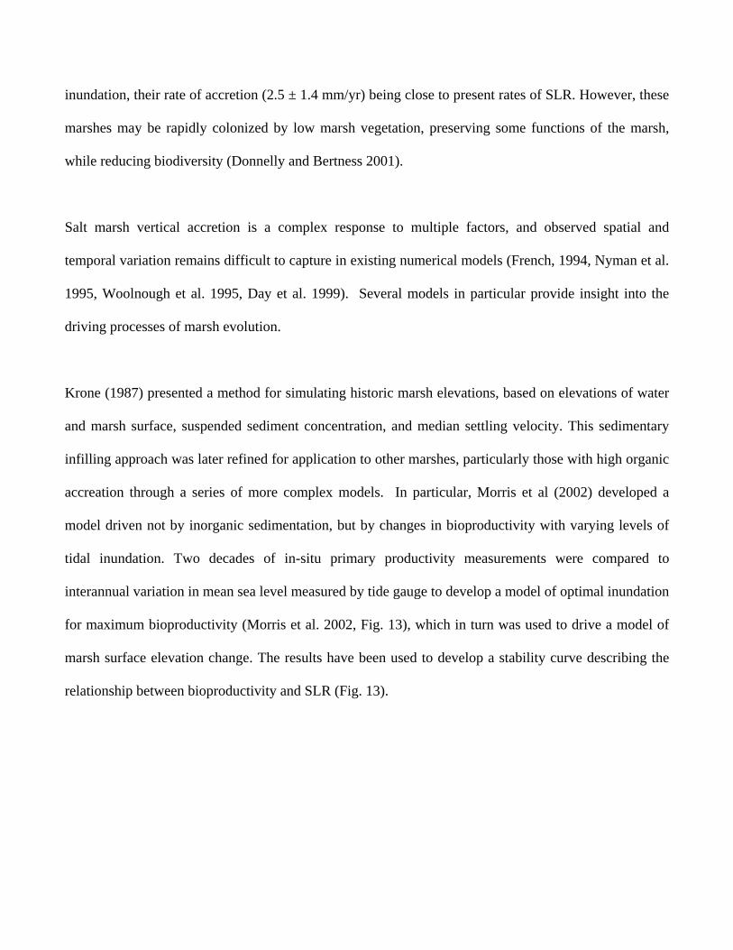
for maximum bioproductivity (Morris et al. 2002, Fig. 13), which in turn was used to drive a model of

marsh surface elevation change. The results have been used to develop a stability curve describing the

relationship between bioproductivity and SLR (Fig. 13).

Rybczyk and Cahoon (2002) employ a cohort modeling approach combined with field data to explore

the submergence potential of two Gulf coast marshes, one stable and one failing. A primary productivity

submodel is intergrated with a complex sediment dynamics submodel forced by mineral sediment influx.

Changes in rates of decomposition, root distribution, sediment compaction, peat characteristics, and

marsh surface elevation were also incorporated. Long-term predictions for the stable site based on the

model suggest that it will not be able to keep up with accelerating rates of RSLR (Rybczyk and Cahoon

2002).

Many models are empirically driven and parameterized based on long-term records from peat cores;

however marsh vertical accretion rates do not necessarily coincide with SLR (French 1994). To counter

this problem, French (2006) proposes a zero-dimensional mass-balance model based on an extensive

data set from published literature, including rates of SLR, tidal range, and sediment supply. The results

show that marshes dominated by inorganic sediment supply are generally near to an equilibrium state

with present rates of SLR; microtidal marshes being the closest to this theoretical equilibrium. The

Figure 13. Observed productivity Spartina alterniflora versus depth of inundation below mean high tide (MHT) of supratidal (open circles) and intertidal (solid circles) marsh sites. Depth below MHT is a highly significant predictor of productivity (r2 = 0.81, P < 0.0001). Solid line represents stable range of equilibrium productivity; dashed line represents instability and reduced productivity. From Morris et al. 2002.

model suggests that marshes dominated by inorganic sediment are more resilient to increases in the rates

of RSLR as tidal range and sediment supply increase (French 2006).

In contrast, a recent simplified 3D model from Kirwan and Murray (2007) demonstrated that the

presence of vegetation stabilized marsh surface elevation relative to SLR, suggesting that rates of

bioproductivity will be able to drive an elevation gain sufficient to keep up with SLR. The model does

not take into account variable patterns of sediment influx and is based on a high rate of bioproductivity,

but is a robust within the constraints of the chosen parameters (Kirwan and Murray 2007).

Marsh inundation with rising sea level

Models are already being applied to policy and management decisions along the U.S. mid-Atlantic

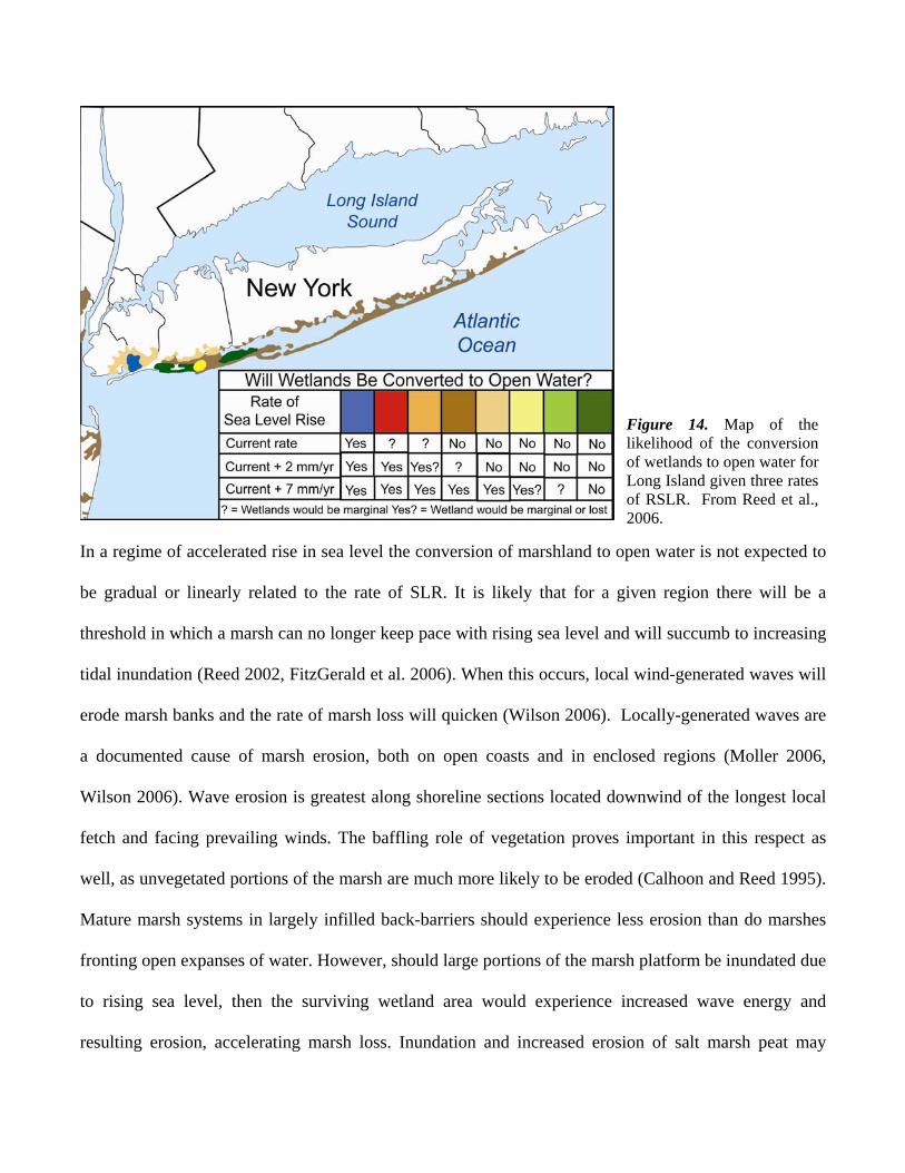
coast. A field-based predictive modeling study by Reed et al. (2006) attempts to utilize the wealth of

published vertical accretion data in concert with tide gauge records to predict regional-scale wetland

inundation into the next century. Within the selected study regions, ranging from Virginia north to New

York, the likelihood of marsh submergence was calculated for three possible RSLR scenarios (Fig. 14).

There was some variation in the quality and resolution of the data used, which were also predominantly

from low marsh sites, potentially skewing sedimentation rates upward. Nevertheless, this report is an

ambitious and valuable contribution to the literature that is especially useful to coastal managers who

must decide where to allocate limited resources within a region. The results suggest that the majority of

mid-Atlantic marshes are stable relative to present rates of SLR, and will vertically accrete at a rate

comparable to accelerated rates of SLR (example: Fig. 14). However, research indicates that there may

be a limit to annual accretion rates (Fig. 11), making this environment extremely vulnerable to the

possible acceleration in SLR (Callaway et al. 1996, Donnelly and Bertness 2001, Reed 2002).

In a regime of accelerated rise in sea level the conversion of marshland to open water is not expected to

be gradual or linearly related to the rate of SLR. It is likely that for a given region there will be a

threshold in which a marsh can no longer keep pace with rising sea level and will succumb to increasing

tidal inundation (Reed 2002, FitzGerald et al. 2006). When this occurs, local wind-generated waves will

erode marsh banks and the rate of marsh loss will quicken (Wilson 2006). Locally-generated waves are

a documented cause of marsh erosion, both on open coasts and in enclosed regions (Moller 2006,

Wilson 2006). Wave erosion is greatest along shoreline sections located downwind of the longest local

fetch and facing prevailing winds. The baffling role of vegetation proves important in this respect as

well, as unvegetated portions of the marsh are much more likely to be eroded (Calhoon and Reed 1995).

Mature marsh systems in largely infilled back-barriers should experience less erosion than do marshes

fronting open expanses of water. However, should large portions of the marsh platform be inundated due

to rising sea level, then the surviving wetland area would experience increased wave energy and

resulting erosion, accelerating marsh loss. Inundation and increased erosion of salt marsh peat may

Figure 14. Map of the likelihood of the conversion of wetlands to open water for Long Island given three rates of RSLR. From Reed et al., 2006.

provide a powerful positive feedback mechanism for increasing greenhouse gases and global warming

by converting organic matter to carbon dioxide and methane (Chmura et al. 2003).

The process whereby marshes are transformed to an open water environment is highly complex, site-

specific, and related to a number of variables including suspended sediment concentrations, nutrient

abundance, storm frequency and intensity, and other factors (Reed 2002). However, gross marsh

morphology will influence the temporal and spatial pattern of marsh inundation (Argow and FitzGerald

2006). Marshes exhibiting a platform-like morphology, such as the high-marsh-dominated coastal

wetlands of New England, could be expected to lose very little areal extent during the initial stages of

increased rates of SLR. However, when mean high water levels eventually exceed the elevation of the

marsh platform, the marsh may be rapidly inundated. Ramped marshes, in contrast, would be expected

to show gradual, persistent loss of aerial extent (or inland migration) in concert with rising sea level

Barataria Bay, Gulf of Mexico, has experienced significant wetlands loss in the past half century with

high rates of RSLR (Barras 1994), and provides an excellent example of this gradual marsh loss,

discussed further below.

BARRIERS AND TIDAL INLETS

Introduction

Barriers comprise approximately 15% of the world's coastlines and are found along every continent

except Antarctica, in every type of geological setting, and in every type of climate (Davies 1980,

Reinson 1984, Davis 1994) They are also best developed in areas of microtidal to mesotidal range1 and

in mid to lower latitudes (Hayes 1979). Climatic conditions control the vegetation on the barriers and in

backbarrier regions, sediment type, and in some regions such as the Arctic, the formation and

modification of barriers themselves.

Barriers are linear features that tend to parallel the coast, generally occurring in groups or chains. The

longest barrier chains in the world coincide with Amero-trailing edges and include the East Coast of the

United States (3100 km) and the Gulf of Mexico coast (1600 km). There are also sizable barrier chains

along the East Coast of South America (960 km), East Coast of India (680 km), North Sea coast of

Europe (560 km), Eastern Siberia (300 km), and the North Slope of Alaska (900 km). Isolated barriers

are common along glaciated coasts such as in northern New England and eastern Canada, and along

high-relief collision coasts, such as the west coast of North and South America. Hayes (1979) has shown

that barrier coastlines can be separated two types based on their wave energy and tidal range1: 1. Wave-

dominated coasts contain long linear barrier islands, few tidal inlets, and open-water lagoons and bays

(i.e. Texas, Panhandle of Florida, Outer Banks of North Carolina, northern New Jersey, Nile River delta,

Fig. 15), 2. Mixed-energy coasts have short, stubby barriers, numerous tidal inlets, and a backbarrier

consisting of marsh and tidal creeks (i.e., Virginia, South Carolina, Georgia, Friesian Islands in the

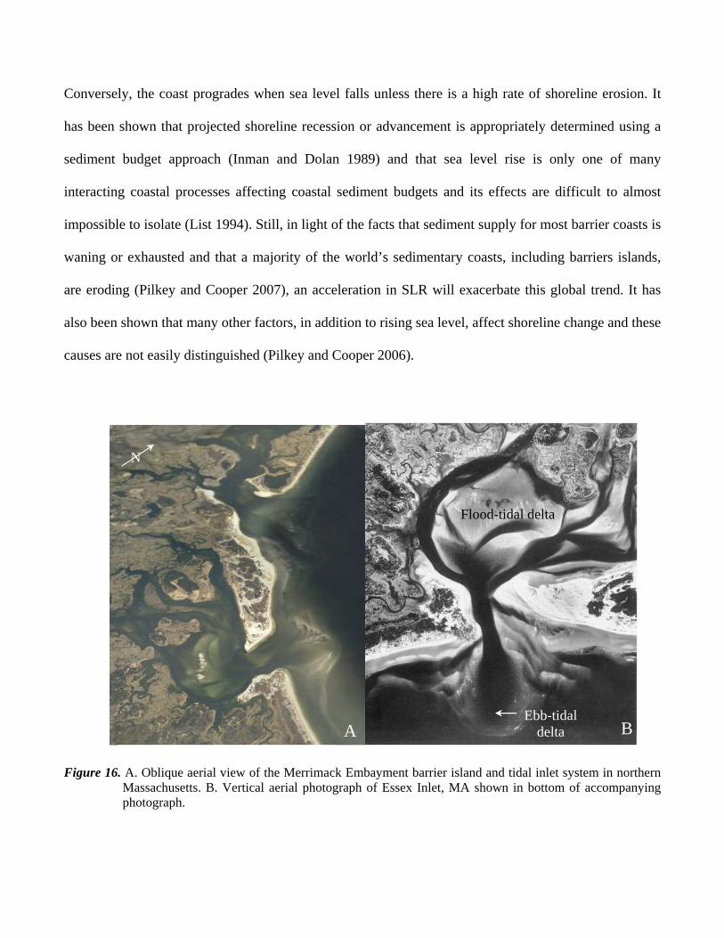
North Sea, Algarve in Portugal, northern New England, Fig. 16).

Tidal inlets are openings along barrier island chains through which water penetrates the land thereby

providing a connection between the ocean and bays, lagoons, and marsh and tidal creek systems. Tidal

currents maintain the main channel of a tidal inlet by continually removing sediment dumped into the

main channel by wave action. Some tidal inlets coincide with the mouths of rivers (estuaries) but in

these cases inlet dimensions and sediment transport trends are still governed, to a large extent, by the

volume of water exchanged at the inlet mouth (tidal prism) and the reversing tidal currents, respectively.

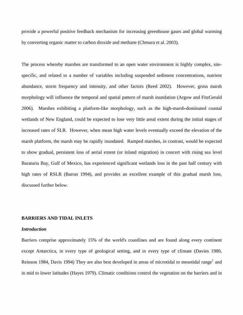
Closely associated with tidal inlets are sand shoals and tidal channels located on the landward and

seaward sides of the inlets. Flood tidal currents deposit sand landward of the inlet forming a flood-tidal

delta and ebb-tidal currents deposit sand on the seaward side forming an ebb-tidal delta (Fig. 16). The

effects of rising sea level on barriers and tidal inlets are treated jointly in this section because of their

complex interactions.

Figure 15. Barrier island and tidal inlet environments (from Pettijohn et al, 1988).

Tidal inlets throughout the world exhibit several consistent relationships that have allowed coastal

engineers and marine geologists to formulate predictive models based on field measurements and

regression analysis. Two of these relationships are particularly useful in predicting how tidal inlets will

respond to accelerated SLR:

Inlet Throat Area - Tidal Prism Relationship- The volume of water flowing through a tidal inlet during a

half tidal cycle, termed the tidal prism (P), is closely related to the inlet throat cross sectional area (Ac)

measured during a spring tide (O’Brien 1931, 1969, Jarrett 1976).

Ac = 7.49 x 10-5 P0.86 (7)

Ebb-Tidal Delta Volume - Tidal Prism Relationship- The spring tidal prism has been shown to closely

correspond to the volume of sand (V) contained in the ebb-tidal delta (Walton and Adams 1976). They

showed that the relationship is improved slightly when wave energy is taken into account.

V = 1.89 x 10-5 P1.23 (8)

Barrier Response to Sea-Level Rise

The response of sedimentary coasts to sea-level changes was discussed in a landmark paper by Curray

(1964) in which he related progradation versus retrogradation2 of a coast to the rate of sea level rise and

whether the supply of sediment to the coast results in erosion or deposition. As Curray (1964) showed,

the coast retreats in most SLR scenarios unless a high rate of sediment deposition offsets this tendency.

2 Curray used the terms transgression for the shoreline retreating landward (retrograding) and regression for a shoreline migrating seaward (prograding).

Conversely, the coast progrades when sea level falls unless there is a high rate of shoreline erosion. It

has been shown that projected shoreline recession or advancement is appropriately determined using a

sediment budget approach (Inman and Dolan 1989) and that sea level rise is only one of many

interacting coastal processes affecting coastal sediment budgets and its effects are difficult to almost

impossible to isolate (List 1994). Still, in light of the facts that sediment supply for most barrier coasts is

waning or exhausted and that a majority of the world’s sedimentary coasts, including barriers islands,

are eroding (Pilkey and Cooper 2007), an acceleration in SLR will exacerbate this global trend. It has

also been shown that many other factors, in addition to rising sea level, affect shoreline change and these

causes are not easily distinguished (Pilkey and Cooper 2006).

Figure 16. A. Oblique aerial view of the Merrimack Embayment barrier island and tidal inlet system in northern Massachusetts. B. Vertical aerial photograph of Essex Inlet, MA shown in bottom of accompanying photograph.

A

B

Flood-tidal delta

Ebb-tidal delta

N

A

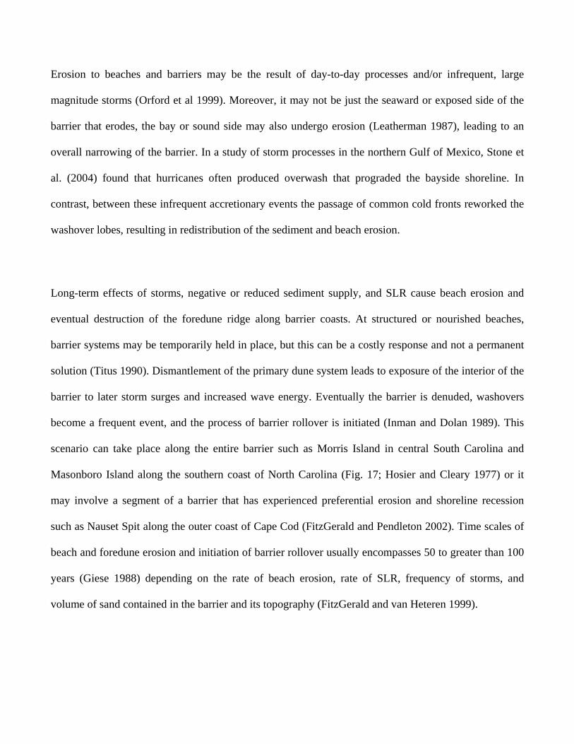
Erosion to beaches and barriers may be the result of day-to-day processes and/or infrequent, large

magnitude storms (Orford et al 1999). Moreover, it may not be just the seaward or exposed side of the

barrier that erodes, the bay or sound side may also undergo erosion (Leatherman 1987), leading to an

overall narrowing of the barrier. In a study of storm processes in the northern Gulf of Mexico, Stone et

al. (2004) found that hurricanes often produced overwash that prograded the bayside shoreline. In

contrast, between these infrequent accretionary events the passage of common cold fronts reworked the

washover lobes, resulting in redistribution of the sediment and beach erosion.

Long-term effects of storms, negative or reduced sediment supply, and SLR cause beach erosion and

eventual destruction of the foredune ridge along barrier coasts. At structured or nourished beaches,

barrier systems may be temporarily held in place, but this can be a costly response and not a permanent

solution (Titus 1990). Dismantlement of the primary dune system leads to exposure of the interior of the

barrier to later storm surges and increased wave energy. Eventually the barrier is denuded, washovers

become a frequent event, and the process of barrier rollover is initiated (Inman and Dolan 1989). This

scenario can take place along the entire barrier such as Morris Island in central South Carolina and

Masonboro Island along the southern coast of North Carolina (Fig. 17; Hosier and Cleary 1977) or it

may involve a segment of a barrier that has experienced preferential erosion and shoreline recession

such as Nauset Spit along the outer coast of Cape Cod (FitzGerald and Pendleton 2002). Time scales of

beach and foredune erosion and initiation of barrier rollover usually encompasses 50 to greater than 100

years (Giese 1988) depending on the rate of beach erosion, rate of SLR, frequency of storms, and

volume of sand contained in the barrier and its topography (FitzGerald and van Heteren 1999).

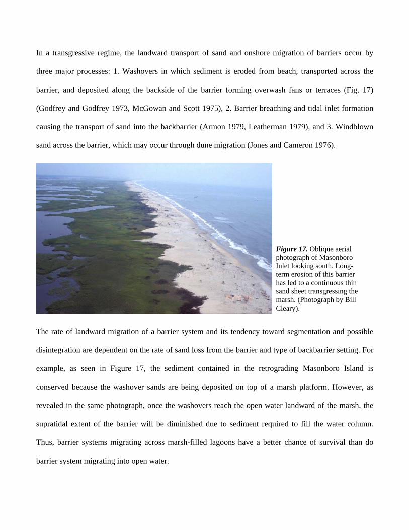
In a transgressive regime, the landward transport of sand and onshore migration of barriers occur by

three major processes: 1. Washovers in which sediment is eroded from beach, transported across the

barrier, and deposited along the backside of the barrier forming overwash fans or terraces (Fig. 17)

(Godfrey and Godfrey 1973, McGowan and Scott 1975), 2. Barrier breaching and tidal inlet formation

causing the transport of sand into the backbarrier (Armon 1979, Leatherman 1979), and 3. Windblown

sand across the barrier, which may occur through dune migration (Jones and Cameron 1976).

The rate of landward migration of a barrier system and its tendency toward segmentation and possible

disintegration are dependent on the rate of sand loss from the barrier and type of backbarrier setting. For

example, as seen in Figure 17, the sediment contained in the retrograding Masonboro Island is

conserved because the washover sands are being deposited on top of a marsh platform. However, as

revealed in the same photograph, once the washovers reach the open water landward of the marsh, the

supratidal extent of the barrier will be diminished due to sediment required to fill the water column.

Thus, barrier systems migrating across marsh-filled lagoons have a better chance of survival than do

barrier system migrating into open water.

Figure 17. Oblique aerial photograph of Masonboro Inlet looking south. Long-term erosion of this barrier has led to a continuous thin sand sheet transgressing the marsh. (Photograph by Bill Cleary).

Causes of Barrier Disintegration

Perhaps one of best-chronicled examples of barrier fragmentation is the Isle Dernieres located along the

central Mississippi River delta coast (Fig. 18). The Isle Dernieres are a barrier arc that formed from the

reworking of an abandoned distributary lobe of the Lafourche delta complex (Bayou Grand Caillou) that

was active from 910 to 400 yrs BP (Penland et al. 1988). In the mid-1800’s the barrier arc was attached

to the mainland, but became separated due SLR and high rates of subsidence (Penland et al. 1981). The

process of barrier arc detachment from the mainland is indicative that the distributary headland no

longer supplied sediment to the barrier system (Penland et al. 1988). As depicted in the sequence of

maps in Fig. 18, rapid subsidence in the region (Penland and Ramsey 1990), the lack of new sediment,

and sediment losses both alongshore and offshore have combined to thin and segment the barrier.

A robust and continuous barrier chain in the mid-1800’s was transformed into a thin, highly

discontinuous barrier system by the late 1900’s necessitating extensive beach nourishment projects to

keep it from disappearing (Kulp et al. 2005). The high rate of relative SLR for this region, which is close

to 1m/century (Penland and Ramsey 1990), provides insight of how barrier chains may respond in a

regime of accelerated SLR. In other locations, barrier segmentation is hastened by barrier breaching and

tidal inlet formation (Giese 1988). When a barrier is breached, the newly formed inlet becomes a

sediment sink as sand is moved seaward and landward building ebb and flood deltas, respectively (Fig.

16). This trapping of sand by the inlet depletes the sand reservoir of the littoral transport system leading

to erosion of the downdrift shoreline. This condition is illustrated along the outer coast of Cape Cod,

Massachusetts, when Nauset Spit was breached during a moderate northeast storm on January 2, 1987

following a long period of beach erosion and barrier thinning caused by a diminished sediment supply

and SLR (Friedrichs et al. 1993, FitzGerald and Pendleton 2002). During the breaching process and

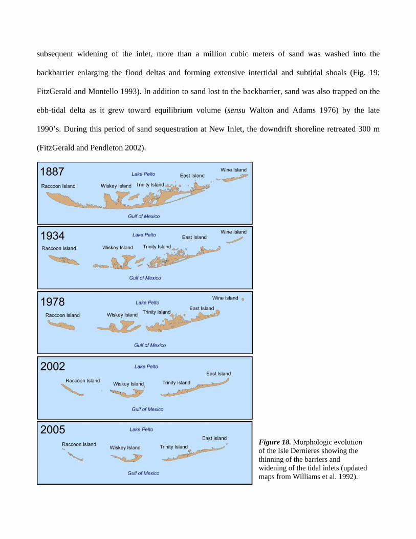
subsequent widening of the inlet, more than a million cubic meters of sand was washed into the

backbarrier enlarging the flood deltas and forming extensive intertidal and subtidal shoals (Fig. 19;

FitzGerald and Montello 1993). In addition to sand lost to the backbarrier, sand was also trapped on the

ebb-tidal delta as it grew toward equilibrium volume (sensu Walton and Adams 1976) by the late

1990’s. During this period of sand sequestration at New Inlet, the downdrift shoreline retreated 300 m

(FitzGerald and Pendleton 2002).

Figure 18. Morphologic evolution of the Isle Dernieres showing the thinning of the barriers and widening of the tidal inlets (updated maps from Williams et al. 1992).

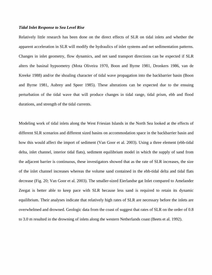
Tidal Inlet Response to Sea Level Rise

Relatively little research has been done on the direct effects of SLR on tidal inlets and whether the

apparent acceleration in SLR will modify the hydraulics of inlet systems and net sedimentation patterns.

Changes in inlet geometry, flow dynamics, and net sand transport directions can be expected if SLR

alters the basinal hypsometry (Mota Oliveira 1970, Boon and Byrne 1981, Dronkers 1986, van de

Kreeke 1988) and/or the shoaling character of tidal wave propagation into the backbarrier basin (Boon

and Byrne 1981, Aubrey and Speer 1985). These alterations can be expected due to the ensuing

perturbation of the tidal wave that will produce changes in tidal range, tidal prism, ebb and flood

durations, and strength of the tidal currents.

Modeling work of tidal inlets along the West Friesian Islands in the North Sea looked at the effects of

different SLR scenarios and different sized basins on accommodation space in the backbarrier basin and

how this would affect the import of sediment (Van Goor et al. 2003). Using a three element (ebb-tidal

delta, inlet channel, interior tidal flats), sediment equilibrium model in which the supply of sand from

the adjacent barrier is continuous, these investigators showed that as the rate of SLR increases, the size

of the inlet channel increases whereas the volume sand contained in the ebb-tidal delta and tidal flats

decrease (Fig. 20; Van Goor et al. 2003). The smaller-sized Eierlandse gat Inlet compared to Amelander

Zeegat is better able to keep pace with SLR because less sand is required to retain its dynamic

equilibrium. Their analyses indicate that relatively high rates of SLR are necessary before the inlets are

overwhelmed and drowned. Geologic data from the coast of suggest that rates of SLR on the order of 0.8

to 3.0 m resulted in the drowning of inlets along the western Netherlands coast (Beets et al. 1992).

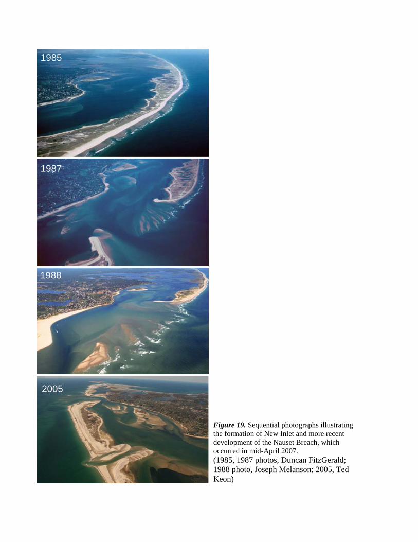
1985

1987

1988

2007

Figure 19. Sequential photographs illustrating the formation of New Inlet and more recent development of the Nauset Breach, which occurred in mid-April 2007. (1985, 1987 photos, Duncan FitzGerald; 1988 photo, Joseph Melanson; 2005, Ted Keon)

2005

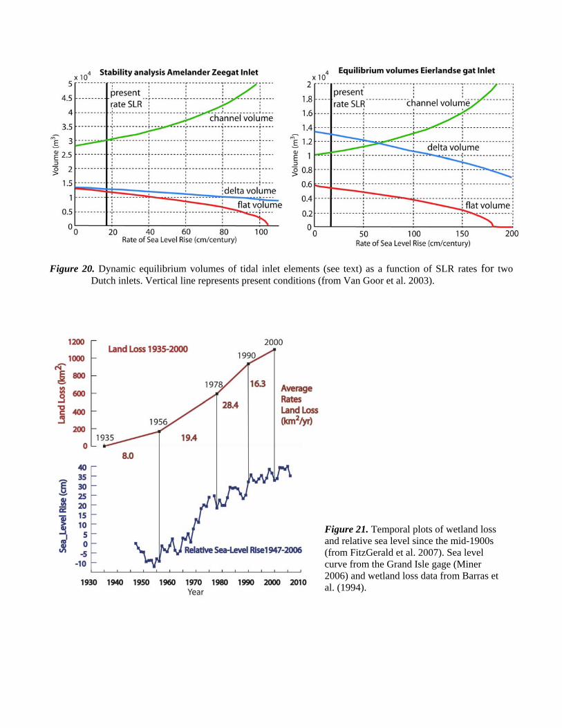
Figure 20. Dynamic equilibrium volumes of tidal inlet elements (see text) as a function of SLR rates for two Dutch inlets. Vertical line represents present conditions (from Van Goor et al. 2003).

Figure 21. Temporal plots of wetland loss and relative sea level since the mid-1900s (from FitzGerald et al. 2007). Sea level curve from the Grand Isle gage (Miner 2006) and wetland loss data from Barras et al. (1994).

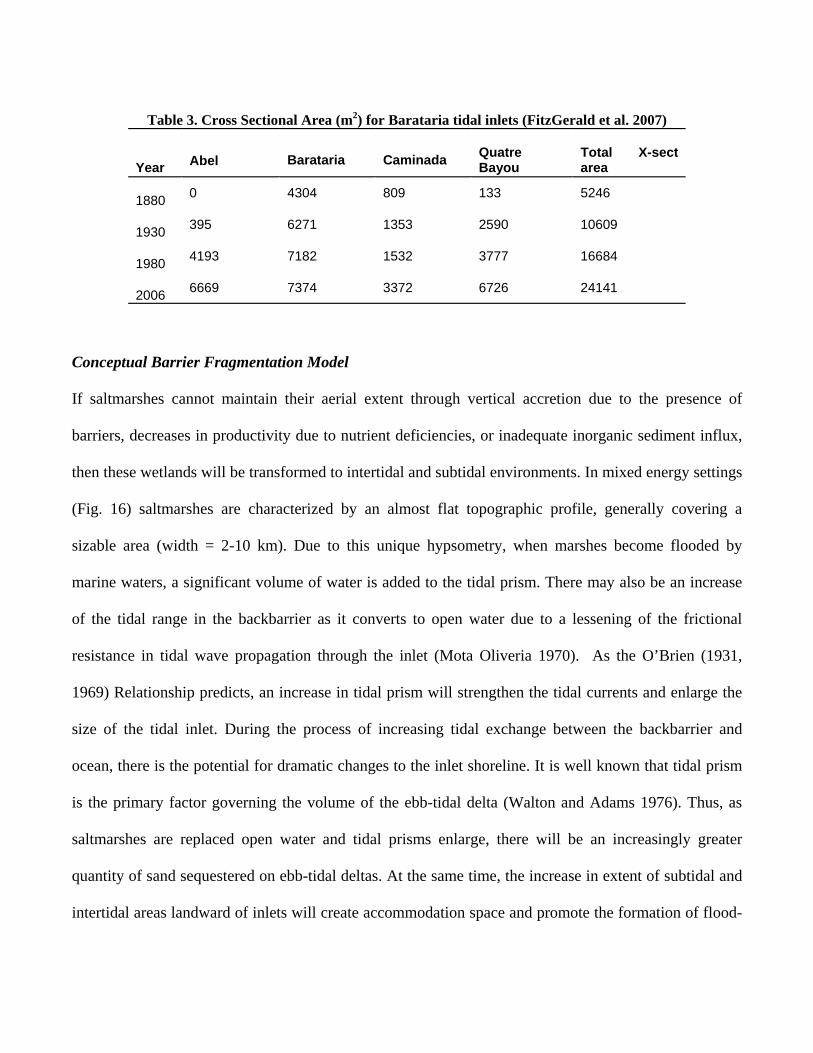
Conceptual Barrier Fragmentation Model

If saltmarshes cannot maintain their aerial extent through vertical accretion due to the presence of

barriers, decreases in productivity due to nutrient deficiencies, or inadequate inorganic sediment influx,

then these wetlands will be transformed to intertidal and subtidal environments. In mixed energy settings

(Fig. 16) saltmarshes are characterized by an almost flat topographic profile, generally covering a

sizable area (width = 2-10 km). Due to this unique hypsometry, when marshes become flooded by

marine waters, a significant volume of water is added to the tidal prism. There may also be an increase

of the tidal range in the backbarrier as it converts to open water due to a lessening of the frictional

resistance in tidal wave propagation through the inlet (Mota Oliveria 1970). As the O’Brien (1931,

1969) Relationship predicts, an increase in tidal prism will strengthen the tidal currents and enlarge the

size of the tidal inlet. During the process of increasing tidal exchange between the backbarrier and

ocean, there is the potential for dramatic changes to the inlet shoreline. It is well known that tidal prism

is the primary factor governing the volume of the ebb-tidal delta (Walton and Adams 1976). Thus, as

saltmarshes are replaced open water and tidal prisms enlarge, there will be an increasingly greater

quantity of sand sequestered on ebb-tidal deltas. At the same time, the increase in extent of subtidal and

intertidal areas landward of inlets will create accommodation space and promote the formation of flood-

Table 3. Cross Sectional Area (m2) for Barataria tidal inlets (FitzGerald et al. 2007) Year

Abel

Barataria

Caminada

Quatre Bayou

Total X-sect area

1880 0 4304 809 133 5246

1930 395 6271 1353 2590 10609

1980 4193 7182 1532 3777 16684

2006 6669 7374 3372 6726 24141

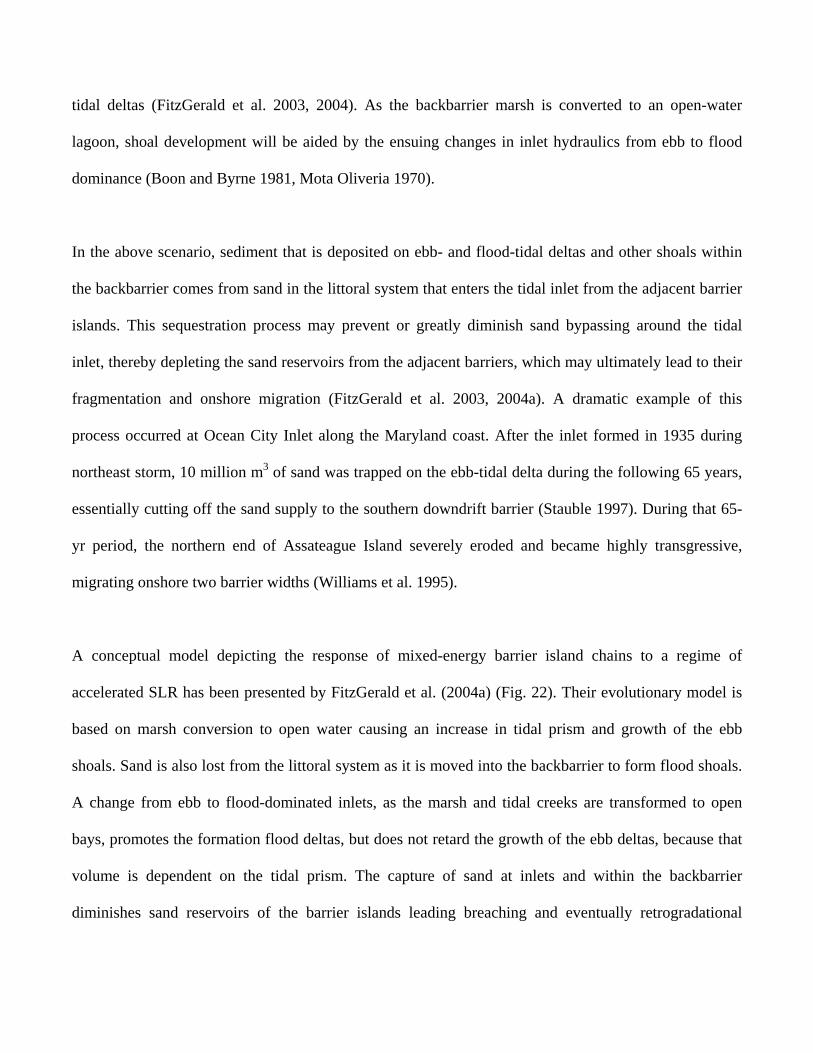
tidal deltas (FitzGerald et al. 2003, 2004). As the backbarrier marsh is converted to an open-water

lagoon, shoal development will be aided by the ensuing changes in inlet hydraulics from ebb to flood

dominance (Boon and Byrne 1981, Mota Oliveria 1970).

In the above scenario, sediment that is deposited on ebb- and flood-tidal deltas and other shoals within

the backbarrier comes from sand in the littoral system that enters the tidal inlet from the adjacent barrier

islands. This sequestration process may prevent or greatly diminish sand bypassing around the tidal

inlet, thereby depleting the sand reservoirs from the adjacent barriers, which may ultimately lead to their

fragmentation and onshore migration (FitzGerald et al. 2003, 2004a). A dramatic example of this

process occurred at Ocean City Inlet along the Maryland coast. After the inlet formed in 1935 during

northeast storm, 10 million m3 of sand was trapped on the ebb-tidal delta during the following 65 years,

essentially cutting off the sand supply to the southern downdrift barrier (Stauble 1997). During that 65-

yr period, the northern end of Assateague Island severely eroded and became highly transgressive,

migrating onshore two barrier widths (Williams et al. 1995).

A conceptual model depicting the response of mixed-energy barrier island chains to a regime of

accelerated SLR has been presented by FitzGerald et al. (2004a) (Fig. 22). Their evolutionary model is

based on marsh conversion to open water causing an increase in tidal prism and growth of the ebb

shoals. Sand is also lost from the littoral system as it is moved into the backbarrier to form flood shoals.

A change from ebb to flood-dominated inlets, as the marsh and tidal creeks are transformed to open

bays, promotes the formation flood deltas, but does not retard the growth of the ebb deltas, because that

volume is dependent on the tidal prism. The capture of sand at inlets and within the backbarrier

diminishes sand reservoirs of the barrier islands leading breaching and eventually retrogradational

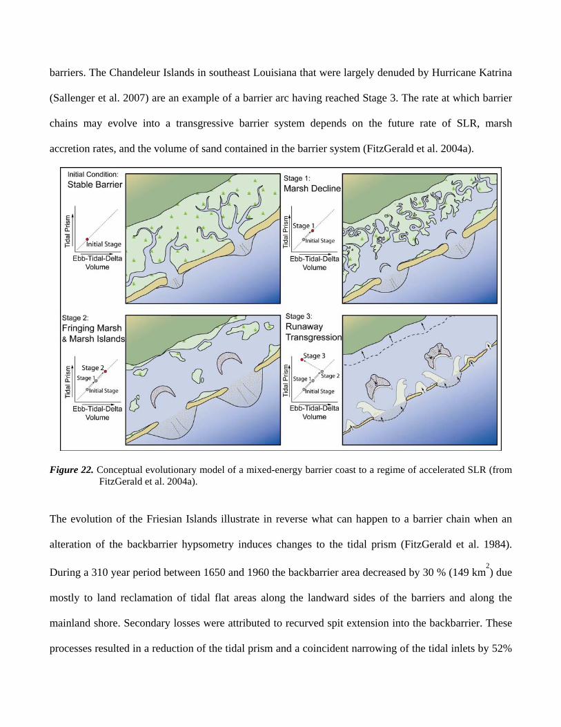
barriers. The Chandeleur Islands in southeast Louisiana that were largely denuded by Hurricane Katrina

(Sallenger et al. 2007) are an example of a barrier arc having reached Stage 3. The rate at which barrier

chains may evolve into a transgressive barrier system depends on the future rate of SLR, marsh

accretion rates, and the volume of sand contained in the barrier system (FitzGerald et al. 2004a).

Figure 22. Conceptual evolutionary model of a mixed-energy barrier coast to a regime of accelerated SLR (from FitzGerald et al. 2004a).

The evolution of the Friesian Islands illustrate in reverse what can happen to a barrier chain when an

alteration of the backbarrier hypsometry induces changes to the tidal prism (FitzGerald et al. 1984).

During a 310 year period between 1650 and 1960 the backbarrier area decreased by 30 % (149 km2) due

mostly to land reclamation of tidal flat areas along the landward sides of the barriers and along the

mainland shore. Secondary losses were attributed to recurved spit extension into the backbarrier. These

processes resulted in a reduction of the tidal prism and a coincident narrowing of the tidal inlets by 52%

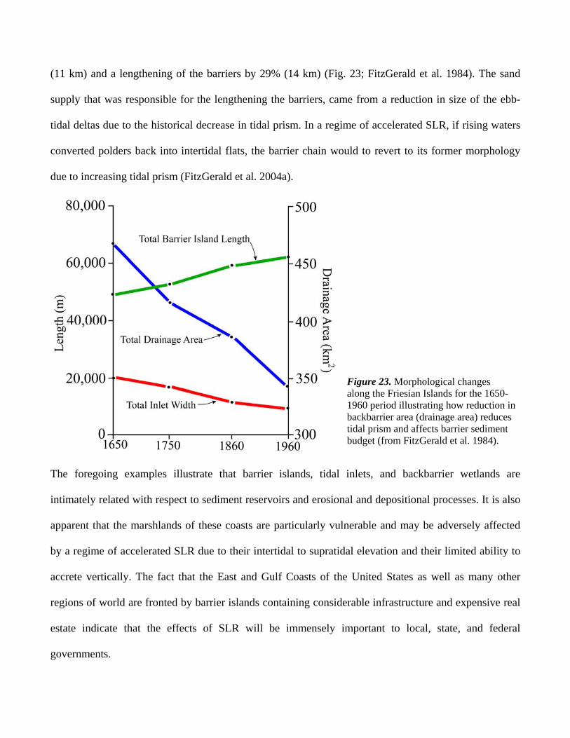
(11 km) and a lengthening of the barriers by 29% (14 km) (Fig. 23; FitzGerald et al. 1984). The sand

supply that was responsible for the lengthening the barriers, came from a reduction in size of the ebb-

tidal deltas due to the historical decrease in tidal prism. In a regime of accelerated SLR, if rising waters

converted polders back into intertidal flats, the barrier chain would to revert to its former morphology

due to increasing tidal prism (FitzGerald et al. 2004a).

The foregoing examples illustrate that barrier islands, tidal inlets, and backbarrier wetlands are

intimately related with respect to sediment reservoirs and erosional and depositional processes. It is also

apparent that the marshlands of these coasts are particularly vulnerable and may be adversely affected

by a regime of accelerated SLR due to their intertidal to supratidal elevation and their limited ability to

accrete vertically. The fact that the East and Gulf Coasts of the United States as well as many other

regions of world are fronted by barrier islands containing considerable infrastructure and expensive real

estate indicate that the effects of SLR will be immensely important to local, state, and federal

governments.

Figure 23. Morphological changes along the Friesian Islands for the 1650-1960 period illustrating how reduction in backbarrier area (drainage area) reduces tidal prism and affects barrier sediment budget (from FitzGerald et al. 1984).

SUMMARY POINTS

1. The advent of accelerated SLR is an ominous byproduct of global warming, and it effects are likely

to be costly both monetarily and in terms of human impact as more than 10% of the world

population lives in coastal regions at elevations lower than 10 m. Many of these regions are

susceptible to gradual inundation, storm flooding, saltwater intrusion, and in some regions,

devastation by tsunamis.

2. A century of research has shown that, over the long term, SLR causes barrier islands to migrate

landward while conserving mass through offshore and onshore sediment transport. Over shorter

time periods, additional factors such as sediment supply and the rate of fluid power expenditure

control the shoreface profile that translates landward during SLR. Under these conditions, coastal

systems adjust to SLR dynamically while maintaining a characteristic geometry that is unique to a

particular coast.

3. Future maintenance of saltmarshes in a regime of SLR is tied to their ability to import inorganic

sediment and produce organic material, particularly root mass. Present estimates of vertical

accretion of high-tide marshes indicate that these environments are highly susceptible to drowning

if SLR accelerates.

4. In a scenario of accelerated SLR, the transformation of backbarrier marshes to open water will

increase tidal prisms resulting in tidal inlet enlargement (leading to erosion of shorelines bordering

inlets) and a growth in size of ebb-tidal deltas (extending shoreline erosion for some distance away

from inlets). Sand will also enter the backbarrier forming flood shoals. This sequestration of sand

on tidal deltas will starve adjacent barrier coasts of sediment, resulting in accelerated erosion.

5. Coastal scientists, engineers, managers, and planners face a great challenge in interpreting the

impact of SLR on beaches and barriers because oceanographic processes work synergistically at a

variety of temporal and spatial scales to produce observable responses. Hydrodynamic and

sediment transport modeling will aid attempts to unravel the impact of different SLR scenarios on

barrier systems. In particular, scientists will need to understand and predict – for different SLR

scenarios – the mobility of beaches and barriers, the sustainability of high and low marshes, the

processes and rates of marsh conversion to open-water areas, and the response times for tidal shoal

development given different rates of tidal prism increase. Understanding and forecasting the

thresholds of barrier and backbarrier stability along both natural and developed coastlines are

among the most vital environmental issues and should be the focus of coastal research for decades

to come.