- 1 -

Choosing the cluster to spli t inbisecting divisive clustering algor ithms

Sergio M. Savaresi†* - Daniel L. Boley‡ - Sergio Bittanti† - Giovanna Gazzaniga††

† Dipartimento di Elettronica e Informazione, Politecnico di Milano, Piazza L. da Vinci, 32, 20133, Milan, ITALY.Phone: +39.02.2399.3545. Fax: +39.02.2399.3412. E-mail: {savaresi,bittanti}@elet.polimi.it.

‡ Department of Electrical Engineering and Computer Science, University of Minnesota, 4-192 EE/CSci, 200 Union StSE, Minneapolis, MN 55455, USA. E-mail:boley@cs.umn.edu.

†† Istituto di Analisi Numerica - C.N.R, Via Ferrata 1, I-27100 PAVIA, ITALY. E-mail: gianna@ian.pv.cnr.it

* Corresponding Author

Abstract. This paper deals with the problem of clustering a data-set. In particular, the bisecting divisive

approach is here considered. This approach can be naturally divided into two sub-problems: the problem

of choosing which cluster must be divided, and the problem of splitt ing the selected cluster. The focus

here is on the first problem. The contribution of this work is to propose a new simple technique for the

selection of the cluster to split. This technique is based upon the shape of the cluster. This result is

presented with reference to two specific split ting algorithms: the celebrated bisecting K-means

algorithm, and the recently proposed Principal Direction Divisive Partitioning (PDDP) algorithm. The

problem of evaluating the quality of a partition is also discussed.

Keywords. Unsupervised clustering; cluster selection; qualit y of clusters; K-means; Principal DirectionDivisive Partitioning.

1. Introduction and problem statement

The problem this paper focuses on is the classical problem of unsupervised clustering of a data-set. In

particular, the bisecting divisive clustering approach is here considered. This approach consists in recursively

spli tting a cluster into two sub-clusters, starting from the main data-set. This is one of the more basic and

common problems in fields li ke pattern analysis, data mining, document retrieval, image segmentation,

decision making, etc. ([GJJ96], [JMF99]).

Note that by recursively using a bisecting divisive clustering procedure, the data-set can be partitioned into

any given number of clusters. Interestingly enough, the so-obtained clusters are structured as a hierarchical

binary tree (or a binary taxonomy). This is the reason why the bisecting divisive approach is very attractive

in many applications (e.g. in document-retrieval/indexing problems – see e.g. [SKV00]).

Any divisive clustering algorithm can be divided into two sub-problems:

- 2 -

x the problem of selecting which cluster must be split;

x the problem of how spli tting the selected cluster.

This paper focuses on the first sub-problem. In particular, in this paper a new method for the selection of the

cluster to spli t is proposed. This method is here presented with reference to two specific bisecting divisive

clustering algorithms:

x the bisecting K-means algorithm;

x the Principal Direction Divisive Partitioning (PDDP) algorithm.

K-means is the most celebrated and widely used clustering technique (see e.g. [F65], [GJJ96], [JD88],

[JMF99], [SI84], [SKV00]); hence it is the best representative of the class of iterative centroid-based divisive

algorithms. On the other hand, PDDP is a recently proposed technique ([B97], [B98], [BG+00a], [BG+00b]).

It is representative of the non-iterative techniques based upon the Singular Value Decomposition (SVD) of a

matrix buil t from the data-set.

The paper is organized as follows: in Section 2 the bisecting K-means and PDDP algorithms are concisely

recalled, whereas in Section 3 the method for the selection of the cluster to spli t is proposed. In Section 4 the

problem of evaluating the quality of a set of clusters is considered and some empirical results are presented.

2. Bisecting K-means and PDDP

The clustering approach considered herein is bisecting divisive clustering. Namely, we want to solve the

problem of splitting the data-matrix > @ NpNxxxM u�� ,...,, 21 (where each column of M, p

ix �� , is a single

data-point) into two sub-matrices (or sub-clusters) LNpLM u�� and RNp

RM u�� , NNN RL � .

This paper focuses on two bisecting divisive partitioning algorithms which belong to different classes of

methods: K-means is the most popular iterative centroid-based divisive algorithm; PDDP is the latest

development of SVD-based partitioning techniques. The specific algorithms considered herein are now

recalled and briefly commented. In such algorithms the definition of “centroid” will be used extensively;

specifically, the centroid of M, say w , is given by

¦

N

jjx

Nw

1

1, (1)

where jx is the j-th column of M . Similarly, the centroids of the sub-clusters LM and RM , say Lw and

Rw , are computed as the average value of their columns.

Bisecting K-means

Step 1. (Initialization). Randomly select a point, say pLc �� ; then compute the centroid w of M, and

compute pRc �� as )( wcwc LR �� .

- 3 -

Step 2. Divide > @NxxxM ,...,, 21 into two sub-clusters LM and RM , according to the following rule:

°°®­

�!���d��

RiLiRi

RiLiLi

cxcxifMx

cxcxifMx

Step 3. Compute the centroids of LM and RM , Lw and Rw .

Step 4. If LL cw and RR cw , stop. Otherwise, let LL wc : , RR wc : and go back to Step 2.

The algorithm above presented is the bisecting version of the general K-means algorithm. This bisecting

algorithm has been recently discussed and emphasized in [SKV00] and [WW+97]. It is here worth noting

that the algorithm above recalled is the very classical and basic version of K-means (except for a slightly

modified initialization step), also known as Forgy’s algorithm ([F65], [GJJ96]). Many variations of this basic

version of the algorithm have been proposed, aiming to reduce the computational demand, at the price of

(hopefully little) sub-optimality.

PDDP

Step 1. Compute the centroid w of M .

Step 2. Compute the auxiliary matrix M~

as weMM � ~, where e is a N-dimensional row vector of ones,

namely > @1,...1,1,1,1,1 e .

Step 3. Compute the Singular Value Decompositions (SVD) of M~

, TVUM 6 ~, where 6 is a diagonal

Npu matrix, and U and V are orthonormal unitary square matrices having dimension ppu and

NNu , respectively (see [GV96] for an exhaustive description of SVD).

Step 4. Take the first column vector of U, say 1Uu , and divide > @NxxxM ,...,, 21 into two sub-clusters

LM and RM , according to the following rule:

°°®­ !��

d��0)(

0)(

wxuifMx

wxuifMx

iT

Ri

iT

Li .

The PDDP algorithm, recently proposed in [B98], belongs to the class of SVD-based data-processing

algorithms ([BDO95], [BDJ99]); among them, the most popular and widely known are the Latent Semantic

Indexing algorithm (LSI – see [A54], [DD+90]), and the LSI-related Linear Least Square Fit (LLSF)

algorithm ([CY95]). PDDP and LSI mainly differ in the fact that the PDDP spli ts the matrix with an

hyperplane passing through its centroid; LSI through the origin. Another major feature of PDDP is that the

SVD of M~

(Step 3.) can be stopped at the first singular value/vector. This makes PDDP significantly less

computationally-demanding than LSI, especially if the data-matrix is sparse and the principal singular vector

is calculated by resorting to the Lanczos technique ( [GV96], [L50]).

The main difference between K-means and PDDP is that K-means is based upon an iterative procedure

- 4 -

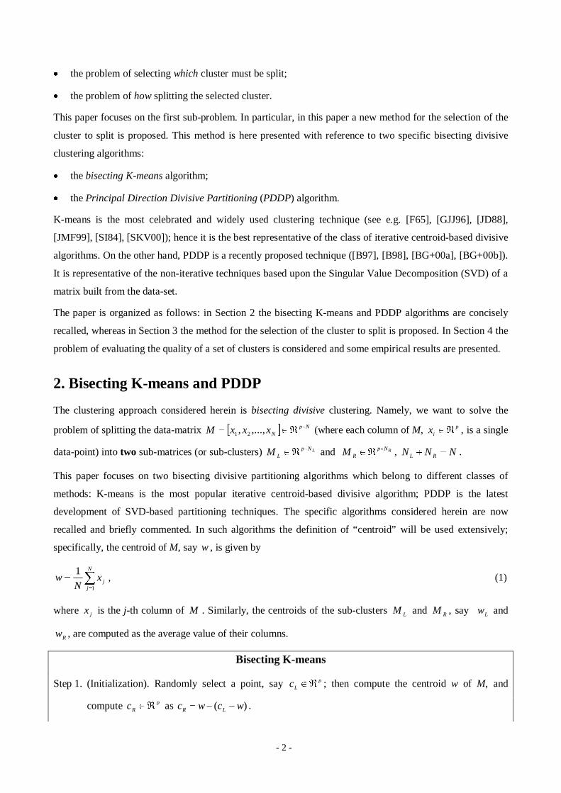
which, in general, provides different results for different initializations, whereas PDDP is a “one-shot”

algorithm which provides a unique solution, given a data-set. In order to understand better how K-means and

PDDP work, in Fig.1a and Fig.1b the partition of a generic matrix of dimension 20002u provided by K-

means and PDDP, respectively, is displayed. From Fig.1, it is easy to see how K-means and PDDP work:

x the bisecting K-means algorithm splits M with an hyperplane which passes through the centroid w of M,

and is perpendicular to the line passing through the centroids Lw and Rw of the sub-clusters LM and

RM . This is due to the fact that the stopping condition for K-means iterations is that each element of a

cluster must be closer to the centroid of that cluster than the centroid of any other cluster.

x PDDP spli ts M with an hyperplane which passes through the centroid w of M, and is perpendicular to the

principal direction of the “unbiased” matrix M~

, which is the translated version of M, having the origin

as centroid. The principal direction of M~

is its direction of maximum variance (see [GV96]).

It is interesting to note that the results of K-means and PDDP are very close, even if the two algorithms differ

substantially (a theoretical explanation of this fact is given and discussed in [SB00]).

K-means and PDDP algorithms, however, provide a solution only to the first sub-problem of bisecting

divisive partitioning: how to spli t a cluster. The problem of selecting which cluster is the best to be split is

left untouched. This wil l be the topic of the following Section.

-1 -0.5 0 0.5 1 1.5

-1

-0.5

0

0.5

1

1.5Bisecting K-means partition

-1 -0.5 0 0.5 1 1.5

-1

-0.5

0

0.5

1

1.5PDDP partition

Fig.1a. Partitioning line (bold) of bisecting K-meansalgorithm. The bullets are the centroids of thedata-set and of the two sub-clusters.

Fig.1b. Partitioning line (bold) of PDDP algorithm. Thebullet is the centroid of the data set. The twoarrows show the principal direction of M

~.

3. Selecting the cluster to spli t

The problem of selecting the cluster to spli t in divisive clustering techniques has received so far much less

attention than what it deserves, since it may have a remarkable impact on the overall clustering results. In the

- 5 -

rest of this section a brief overview on the existing approaches will be given in Subsection 3.1; a new method

for cluster selection will be presented in Subsection 3.2, and discussed in Subsection 3.3.

3.1. Selecting the cluster to split: a quick overview

The following three approaches are typically used for the selection of the cluster to spli t ([JD88]):

(A) complete partition: every cluster is spli t, so obtaining a complete binary tree;

(B) the cluster having the largest number of elements is spli t;

(C) the cluster with the highest var iance with respect to its centroid

¦

� N

jj wx

NM

1

21)(D (2)

is spli t (w is the centroid of data-matrix of the cluster, xj its j-th column, � is the Euclidean norm).

The above criteria are extremely simple and raw. Criterion A) is indeed a "non-choice", since every cluster is

spli t: it has the advantage of providing a complete tree, but it completely ignores the issue of the quality of

the clusters. Criterion B) is also very simple: it does not provide a complete tree, but it has the advantage of

yielding a “balanced” tree, namely a tree where the leaves are (approximately) of the same size. Criterion C)

is the most “sophisticated”, since it is based upon a simple but meaningful property (the "scatter") of a

cluster. This is the reason why C) is the most commonly used criterion for cluster selection.

-1.5 -1 -0.5 0 0.5 1 1.5-1.5

-1

-0.5

0

0.5

1

1.5

N=2000; D(M)=0.53

-1.5 -1 -0.5 0 0.5 1 1.5-1.5

-1

-0.5

0

0.5

1

1.5

N=1000; D(M)=0.10

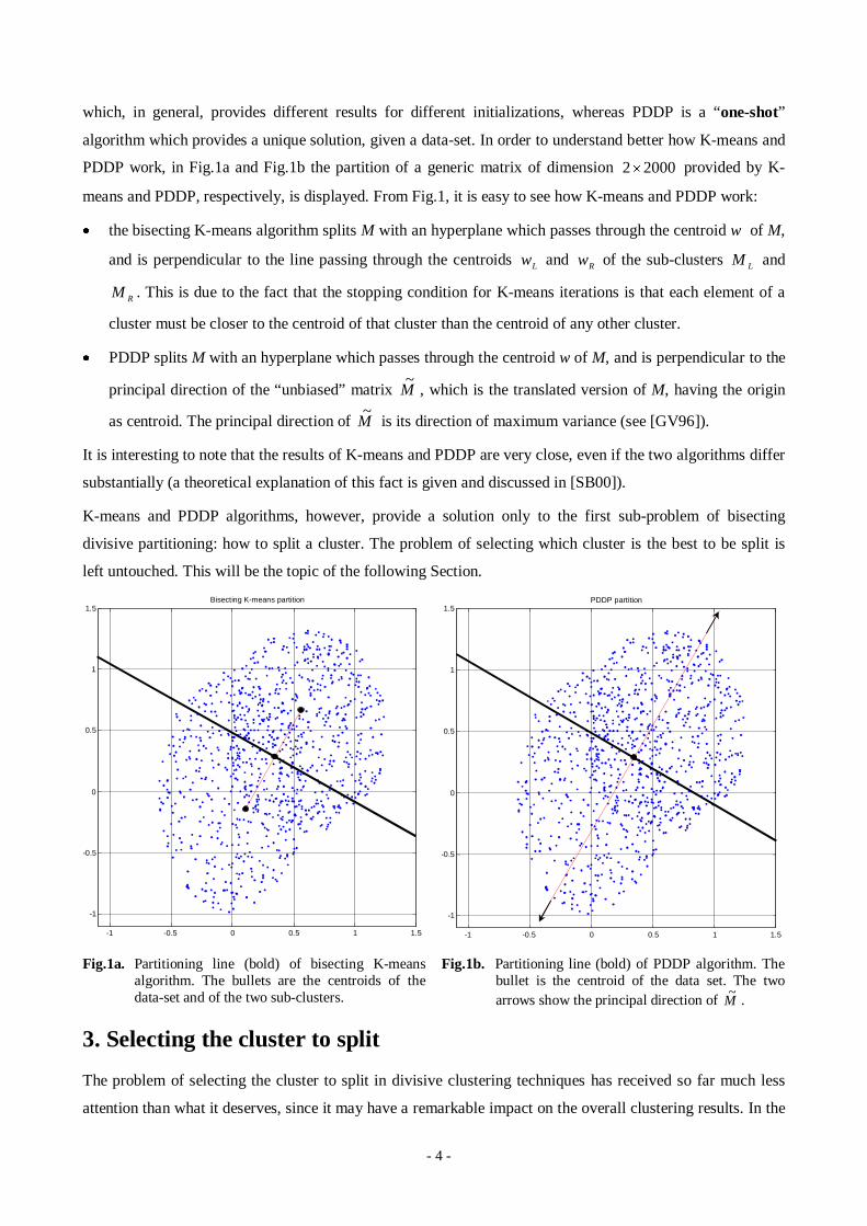
Fig.2a. A data-set with 2000 data-points. Fig.2b. A data-set with 1000 data-points.

The main limit of the above criteria can be pictoriall y described with a naive example. In Fig.2 two data-sets

are displayed: the first is a matrix of size 2u2000 (Fig.2a); the second is a matrix of size 2u1000 (Fig.2b). By

inspecting the two data-sets, it is apparent that the best cluster to spli t is the second one: it is inherently

structured into two sub-clusters. Both criterion B) and C), however, would suggest the first one as the best

- 6 -

cluster to spli t: it has the largest number of data-points, and the largest variance ( 53.0)( MD for the first

data-set, and 10.0)( MD for the second data-set).

It is interesting to observe that the main limit of criteria A)-C) is that they completely ignore the “ shape” of

the cluster, which is known to be a key indicator of the extent to which a cluster is well-suited to be

partitioned into two sub-clusters. This simple but crucial observation, however, deserves some additional

comments:

x taking into account the “shape” of the cluster is a difficult and slippery task, which inherently requires

more computational power than the computation of the simple criterion (2). Henceforth, in

computationally-intensive applications the simplicity of criteria A)-C) can be attractive; however, in

many applications characterized by a comparative small number of data-points (N) and features (p), a

better criterion than A)-C) would be appealing.

x taking into account the “shape” of the cluster requires a wise balancing between an application-specific

approach, and a multi-purpose approach. If the criterion is too application-specific it can only be helpful

for that application. If too generic (as A)-C) are), it cannot provide high clustering performance.

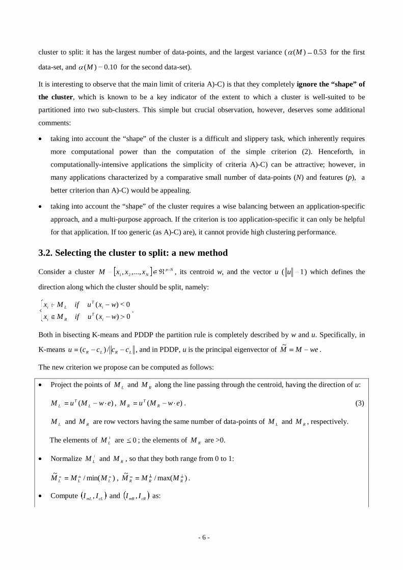
3.2. Selecting the cluster to split: a new method

Consider a cluster > @ NpNxxxM u�� ,...,, 21 , its centroid w, and the vector u ( 1 u ) which defines the

direction along which the cluster should be split, namely:

°°®­ !��

d��0)(

0)(

wxuifMx

wxuifMx

iT

Ri

iT

Li .

Both in bisecting K-means and PDDP the partition rule is completely described by w and u. Specifically, in

K-means LRLR ccccu �� /)( , and in PDDP, u is the principal eigenvector of weMM � ~.

The new criterion we propose can be computed as follows:

x Project the points of LM and RM along the line passing through the centroid, having the direction of u:

)( ewMuM LT

L �� A , )( ewMuM RT

R �� A . (3)

ALM and A

RM are row vectors having the same number of data-points of LM and RM , respectively.

The elements of ALM are 0d ; the elements of A

RM are >0.

x Normalize ALM and A

RM , so that they both range from 0 to 1:

)min(/~ AAA LLL MMM , )max(/

~ AAA RRR MMM .

x Compute � �cLmL II , and � �cRmR II , as:

- 7 -

� � ¸¹·

¨©§ � ¦

ALk

jLLj

L

LcLmL wMk

wII1

22 )~~(

1,)~(, , � � ¸¹

·¨©§ � ¦

ARk

jRRj

R

RcRmR wMk

wII1

22 )~~(

1,)~(, ,

where Lw~ and Rw~ are the centroids of ALM~ and A

RM~ , Lk and Rk are the dimensions of ALM~ and A

RM~ ,

ALjM~ and A

RjM~ are the j-th elements of ALM~ and A

RM~ , respectively.

x Compute ( mI , cI ) =( )(5.0 mRmL II � , )(5.0 cRcL II � ).

x Compute the criterion, denoted )(MJ , as:

m

c

I

IM )(J . (4)

If aM and bM are two clusters, and )()( ba MM JJ � , aM is more suited to be partitioned than bM .

Note that the meaning of )(MJ is intuitive; it is the ratio between the average variance of ALM

~ and A

RM~

around their centroids, and the average squared values of their centroids. ALM

~ and A

RM~

are the normalized

sub-clusters LM and RM projected along the line passing through the centroid with direction u.

3.3. Discussion

The method for cluster selection presented above can be briefly commented as follows:

x Note that neither the scatter of M (given by (2)) nor the distance between the centroids of its sub-clusters

provide useful information about the shape of the data-set M. Indeed, the ratio between scatter and

centroid distance is the indicator that really matters. Indeed, if )(MJ is small, the cluster is expected to

be constituted by two clearly separated sub-clusters, since their scatter is small with respect to their

centroids distance. On the other hand, if )(MJ is large, the cluster cannot be clearly partitioned, since

the two sub-clusters are close and scattered. Criterion )(MJ hence is expected to be a concise but good

indicator of the shape of the cluster.

x Indicator (4) summarizes the properties of the cluster projected along a 1-dimensional line (defined by

u). Of course, this is a limitation with respect to a p-dimensional shape analysis of M. However, note that

this provides the best compromise between computational complexity and shape-information, since u is

the direction of maximum variance of the cluster (this property holds only approximately for K-means -

see [SB00]).

x At a first glance, the fact that M must be split in order to compute )(MJ may appear nonsensical: indeed

the role of )(MJ is to tell us which cluster must be split. This issue deserves some comments:

- as already said, the calculation of a shape-indicator for M is inherently a computational-demanding

task. However, among the many different ways of doing this, )(MJ has the major advantage that, if

M is selected, no additional computation are required. Note that this is not guaranteed for a generic

- 8 -

shape-indicator (in other words, the efforts spent to compute )(MJ can be somehow "recycled").

- if the bisecting clustering recursive procedure is stopped when the data-set has been partitioned into

K sub-clusters, it is easy to see that the computation of )(MJ has required K-1 "useless" bisecting

partitions. However, note that this has li ttle impact on the overall computational balance, since such

partitions are made at "leaves-level" (namely they are partitions of small clusters). Low-level

partitions are known to be much less demanding than high-level partitions.

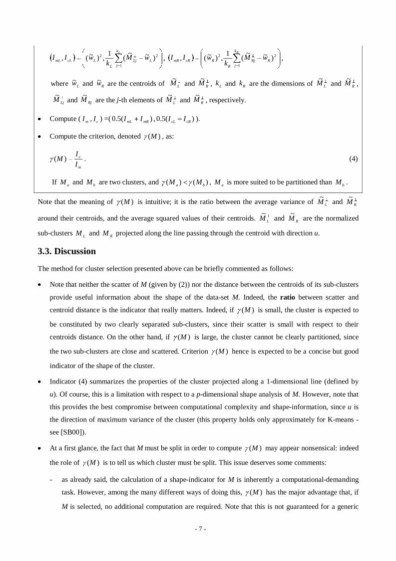
x The shape-indicator (4) can be given a simple but interesting graphical interpretation. On the 2-

dimensional space where the abscissae is given by the average centroid distance from the splitting line

( mI ), and the ordinate is given by the average scatter of the sub-cluster ( cI ), )(MJ is the slope of the

line passing through the origin and the point ( mI , cI ). The smaller this slope is, the more suited M is to

be split. Moreover, it can be proven that, whatever M is, the point ( mI , cI ) lies within a compact convex

2-dimensional interval bounded by the lines cI =0 and mmc III � (and 10 dd mI ). This domain is

depicted in Fig.3 (the computation of this is non-trivial; it is extensively described in [S00]).

0 0.1 0.2 0.3 0.4 0.5 0.6 0.7 0.8 0.9 10

0.05

0.1

0.15

0.2

0.25

Im

Is

mmc III �

),( cm II

Best clusterto split

Fig.3. Domain of points ( mI , cI ).

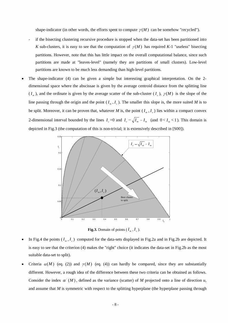
x In Fig.4 the points ( mI , cI ) computed for the data-sets displayed in Fig.2a and in Fig.2b are depicted. It

is easy to see that the criterion (4) makes the "right" choice (it indicates the data-set in Fig.2b as the most

suitable data-set to spli t).

x Criteria )(MD (eq. (2)) and )(MJ (eq. (4)) can hardly be compared, since they are substantially

different. However, a rough idea of the difference between these two criteria can be obtained as follows.

Consider the index )(MAD , defined as the variance (scatter) of M projected onto a line of direction u,

and assume that M is symmetric with respect to the splitting hyperplane (the hyperplane passing through

- 9 -

w and perpendicular to u). Henceforth, )max()min(: AA RL MMv . Under these assumptions, it is easy to

see that the variance of AM (the projection of M along u) is equal to the sum of the variance of ALM , the

variance of ARM , and the squared distances of the centroids of A

LM and ARM from the centroid of AM .

Given the definitions of mI and cI , )(MAD can be therefore re-written as:

)(2)( 2cm IIvM � AD . (5)

Equation (5) is interesting since (even if it holds under some restrictive assumptions) provides a

relationship between )(MJ and a performance index ( )(MAD )closely related to )(MD .

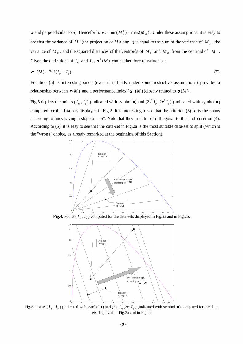
Fig.5 depicts the points ( mI , cI ) (indicated with symbol x) and (2v2mI ,2v2

cI ) (indicated with symbol �)

computed for the data-sets displayed in Fig.2. It is interesting to see that the criterion (5) sorts the points

according to lines having a slope of -45°. Note that they are almost orthogonal to those of criterion (4).

According to (5), it is easy to see that the data-set in Fig.2a is the most suitable data-set to spli t (which is

the "wrong" choice, as already remarked at the beginning of this Section).

0 0.1 0.2 0.3 0.4 0.5 0.6 0.7 0.8 0.9 10

0.05

0.1

0.15

0.2

0.25

Im

Ic

Data-setof Fig.2a

Best cluster to splitaccording to )(MJ

Data-setof Fig.2b

Fig.4. Points ( mI , cI ) computed for the data-sets displayed in Fig.2a and in Fig.2b.

0 0.1 0.2 0.3 0.4 0.5 0.6 0.7 0.8 0.9 10

0.05

0.1

0.15

0.2

0.25

Im

IC

Data-setof Fig.2a

Data-setof Fig.2b

Best cluster to split

according to )(M

AD

Fig.5. Points ( mI , cI ) (indicated with symbol x) and (2v2mI ,2v2

cI ) (indicated with symbol �) computed for the data-sets displayed in Fig.2a and in Fig.2b.

- 10 -

4. Exper imental results

In this section, the selection method proposed in Section 3 wil l be experimentally tested on a set of real data.

This will be done in Subsection 4.2. In Subsection 4.1 a key preliminary issue wil l be discussed: how to

evaluate the performance of a clustering process.

4.1. Per formance evaluation

When a new clustering algorithm or a modification of an existing algorithm is proposed, a crucial problem is

to understand if, and to which extent, this algorithm provides better performance. This is a very subtle and

slippery problem, which, unfortunately, is usually glossed over or de-emphasized. The goal of this

subsection is to present a framework for this problem, and to propose a way of measuring the quality of a

clustering process.

DATA-SET

Partitionmade byexpert

Matrix ofnumbers

Pre-processedmatrix (after

scaling,filtering,

"cleaning", etc.)

Partitionmade byalgorithm

)HDWXUHVVHOHFWLRQ

3UH�SURFHVVLQJ

&OXVWHULQJDOJRULWKP

+XPDQ�H[SHUW��

(;7(51$/TXDOLW\

HYDOXDWLRQ

,17(51$/TXDOLW\

HYDOXDWLRQ

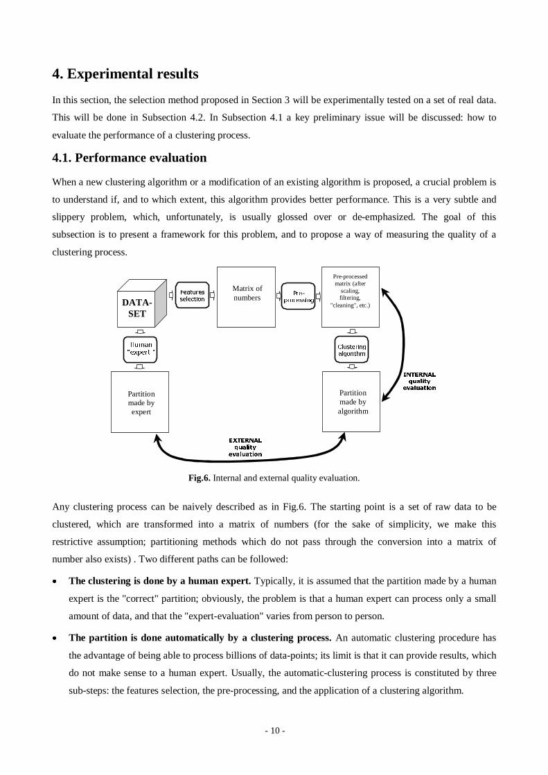
Fig.6. Internal and external quality evaluation.

Any clustering process can be naively described as in Fig.6. The starting point is a set of raw data to be

clustered, which are transformed into a matrix of numbers (for the sake of simplicity, we make this

restrictive assumption; partitioning methods which do not pass through the conversion into a matrix of

number also exists) . Two different paths can be followed:

x The cluster ing is done by a human expert. Typically, it is assumed that the partition made by a human

expert is the "correct" partition; obviously, the problem is that a human expert can process only a small

amount of data, and that the "expert-evaluation" varies from person to person.

x The partition is done automatically by a cluster ing process. An automatic clustering procedure has

the advantage of being able to process billions of data-points; its limit is that it can provide results, which

do not make sense to a human expert. Usually, the automatic-clustering process is constituted by three

sub-steps: the features selection, the pre-processing, and the application of a clustering algorithm.

- 11 -

The evaluation of the results obtained by an automatic clustering procedure can be done in two different

ways (see Fig.6):

x Evaluation of the external quality. In this case, an automatic clustering procedure is assumed to be

good if it provides the same partition yielded by a human expert. A figure of merit for the external

quality of the partition hence is a measure of "distance" between the expert-generated and the algorithm-

generated partitions. Entropy ([BG+00a]) is a widely used measure of external quality.

x Evaluation of the internal quality. In this case, no expert-generated partition is assumed to be

available, nor external information. In this case, only the clustering algorithm (not the entire clustering

process, including feature selection and pre-processing) is evaluated.

Merits and pitfalls of internal and external figures of merit can be summarized as follows:

x Maximizing the external quality is the final goal in any clustering practical application. As a matter of

fact the results obtained by the automatic clustering procedure must be validated by a human expert, in

order to be meaningful and actionable. The main limit of external quality evaluation is that it is

"subjective", since it is strongly dependent on a human-driven clustering process, and on human-driven

steps like features selection and pre-processing. External quality indices hence must be used when

dealing with a specific application. External quality instead can be strongly misleading when the goal is

a general quality assessment of a clustering algorithm.

x Using internal quality is the best way of measuring the performance of clustering algorithm. Obviously,

high internal quality of the algorithm cannot guarantee good results of the overall clustering process in a

specific application, since such results also depend on critical steps like features selection and

preprocessing.

In this paper we have proposed a general method for improving the performance of bisecting divisive

clustering algorithms. This result is general, purely algorithmic, and it is not linked to any specific

application. The natural way of evaluating this method hence is to use an internal quality index.

Given the K matrices ^ `KMMM ,...,, 21 , which constitute a partition of the data-matrix M, the internal quali ty

of the partition can be measured according to the following performance index (see e.g. [JMF99], [SI84],

[SKV00]):

¦¦¦���

������ Kiii Mx

KiMx

iMx

iK wxwxwxMMMJ22

2

2

121 ...),...,,(21

, (6)

where Kwww ,..., 21 are the centroids of ^ `KMMM ,...,, 21 , and ix is the i-th column of M. Note that (6) is a

measure of cohesiveness of each cluster to its centroid: the smaller ),...,,( 21 KMMMJ is, the better is the

partition. This way of measuring the quality of a partition is, however, raw and incomplete. To understand

better how an accurate measure of quali ty should be designed, the general standard definition of a clustering

problem is worth to be recalled.

- 12 -

Definition of an unsupervised cluster ing problem

Given a matrix M, the unsupervised clustering of M into K sub-matrices consists in partitioning M into

^ `KMMM ,...,, 21 ( � � ji MM if ji z , MM j � ), without a-priori or external information, in order to

maximize the similarity among the elements of each sub-matrix (intra-similarity), and to minimize the

similarity among elements of different sub-matrices (inter-similarity).

Note that, according to the above definition, the performance index (6) is incomplete: it only evaluates the

"intra-similarity", without paying attention to "inter-similarity". Given M and ^ `KMMM ,...,, 21 , a more

sophisticated performance index can be computed as follows.

x Compute the scatter, say ^ `Ksss ,...,, 21 , of each sub-matrix about its centroid. In the scatter the

information about "intra-similarity" is condensed. The scatter is of iM is defined as:

¦

� ik

jiji

i

i wMk

s1

2

,

1, (7)

where iw is the centroid of iM , ik is the number of columns of iM , and jiM , is the j-th column of iM .

x Compute the distance, say ^ `Kddd ,...,, 21 , of each sub-matrix from the the others. In id the information

about the "inter-similarity" of iM with respect to the rest of the partition is condensed. The distance id

can be defined as follows:

)(min ijji dd , where )(min ,,, hjkikhij MMd � j,h,k = 1,2,…,K, (8)

where � is the Euclidean norm applied to the columns of matrices (note that ijd is the inter-cluster

distance used in "single-linkage" agglomeration methods) .

x Compute the relative weight, say ^ `KGGG ,...,, 21 , of each sub-matrix. It can be defined as follows:

N

kii G , (9)

where ik is the number of columns of iM , and ¦ i

ikN .

x Compute the performance index � �KMMMQ ,...,, 21 as follows:

� � ¦

K

i i

iiK d

sMMMQ

121 ,...,, G . (10)

The smaller � �KMMMQ ,...,, 21 is, the better the partition.

Performance index (10) is very intuitive: it is the weighted average (the weights being the relative size of

each matrix) of the ratio between scatter and distance. Note that (10) improves (6) since it takes into account

the "inter-similarity" among sub-matrices (according to the definition of a clustering problem) and also

- 13 -

weights the "importance" of each cluster. In the rest of this section (10) wil l be used.

We conclude this subsection with a remark. It is worth pointing out that clustering M by direct minimization

of � �KMMMQ ,...,, 21 (or ),...,,( 21 KMMMJ ) would be, conceptually, the best clustering method.

Unfortunately, the minimization of � �KMMMQ ,...,, 21 requires exhaustive search which is exponential in

time with respect to the number of data-points. Note that the clustering algorithms which have been proposed

in the literature (including K-means and PDDP) can be interpreted as alternate ways of tackling the problem

of minimizing � �KMMMQ ,...,, 21 . All of them provide a solution with a reasonable computational effort, at

the price of some sub-optimality.

4.2. A numerical example

The goal of this subsection is to test the effectiveness of the method for the selection of the cluster to spli t,

presented in Section 3. The method wil l be tested both on bisecting K-means and PDDP, and the results will

be evaluated according to the performance index (10).

Var iable Var iable descr iption1 Major-axis diameter (in arcseconds) from O plate image2 Integrated magnitude from O plate image

3 Magnitude from O plate image using D-M relation for stars4 Major-axis position angle (N to E) from O plate image

5 Ellipticity from O plate image

6 Second Moment of O plate image7 Percent saturation of O plate image

8 Average transmittance of O plate image9 Mean surface brightness (in mag/asec 2) of O plate image

10 Effective (half-li ght) radius from O11 C31 concentration index from O plate.The ratio of the 100% light radius to 50% light radius

12 C32 concentration index from O plate.The ratio of the 100% light radius to 75% light radius13 C21 concentration index from O plate.The ratio of the 75% light radius to 50% light radius

14 Major-axis diameter (in arcseconds) from E plate image15 Integrated magnitude from E plate image

16 Magnitude from E plate image using D-M relation for stars17 Major-axis position angle (N to E) from E plate image

18 Ellipticity from E plate image

19 Second Moment of E plate image20 Percent saturation of E plate image

21 Average transmittance of E plate image22 Mean surface brightness (in mag/asec 2) of E plate image

23 Effective (half-li ght) radius from E24 C31 concentration index from E plate.The ratio of the 100% light radius to 50% light radius

25 C32 concentration index from E plate.The ratio of the 100% light radius to 75% light radius26 C21 concentration index from E plate.The ratio of the 75% light radius to 50% light radius

27 E(B-V) determined by bilinear interpolation of Burstein & Heiles [1982] extinction estimates.28 E(B-V) determined from Schlegel, etal [1998] extinction estimates.

29 O and E imgpars flags (10*Oflag + Eflag).30 O-E color of the object computed using intergrated magnitudes.

31 O-E color of the object computed using D-M relation magnitudes.

32 Estimated local surface density of MAPS-NGP galaxies (in galaxies/degree 2)

Table 1. Features description.

- 14 -

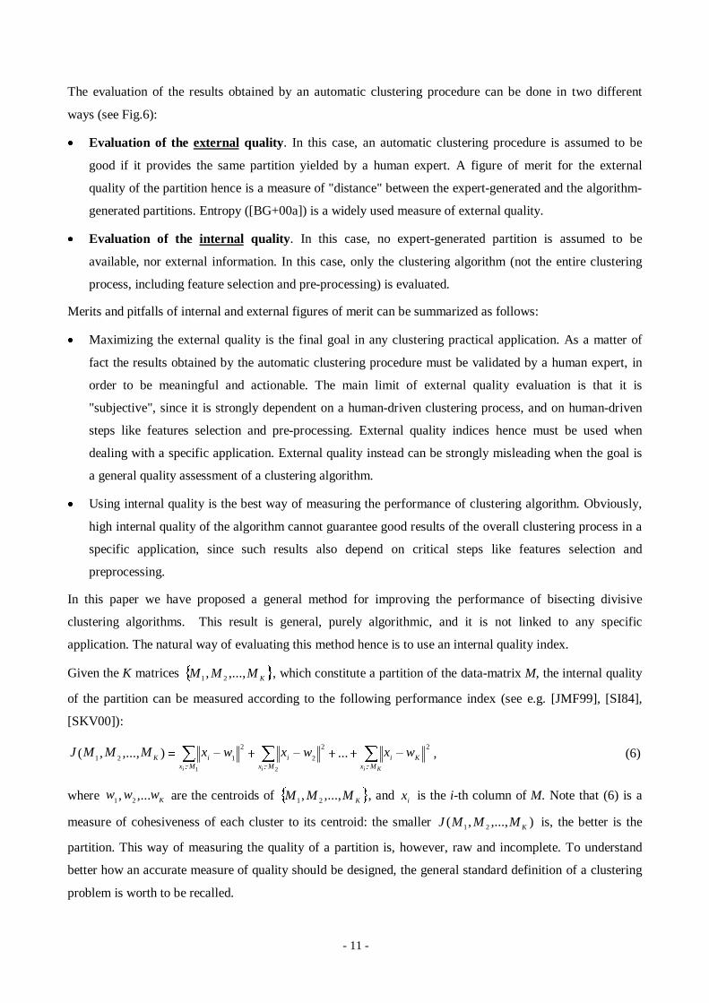
The data-set we have used as a benchmark is a 32u16000 matrix, buil t from 16000 objects extracted from a

database of the University of Minnesota, consisting in a MAPS-NGP catalog of galaxies images on POSS I

(Palomar Observatory Sky Survey) plates within 30 degrees of the North Galactic Pole. The list of the 32

features condensing the information embedded in each image is listed in Table 1. Each feature has been

normalized within the range [-1;+1]. Since our goal here is internal-quali ty evaluation, no further details on

the data-set wil l be given. Detailed information on the data can be found in [C99], [PH+93], or at the URL

http://lua.stcloudstate.edu/~juan/.

50 100 150 200 2500.8

0.9

1

1.1

1.2

1.3

1.4

1.5

Number K of sub-clusters

Quality Q of partition (better partition for lower values of Q) - Bisecting K-means

(B)(C)

(D)

Fig.7. Internal quality evaluation of a partition obtained using bisecting K-means and selection methods (a)-(c).

50 100 150 200 2500.8

0.9

1

1.1

1.2

1.3

1.4

1.5

Number K of sub-clusters

(B)

(C)

(D)

Quality Q of partition (better partition for lower values of Q) - PDDP

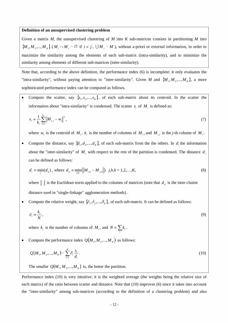
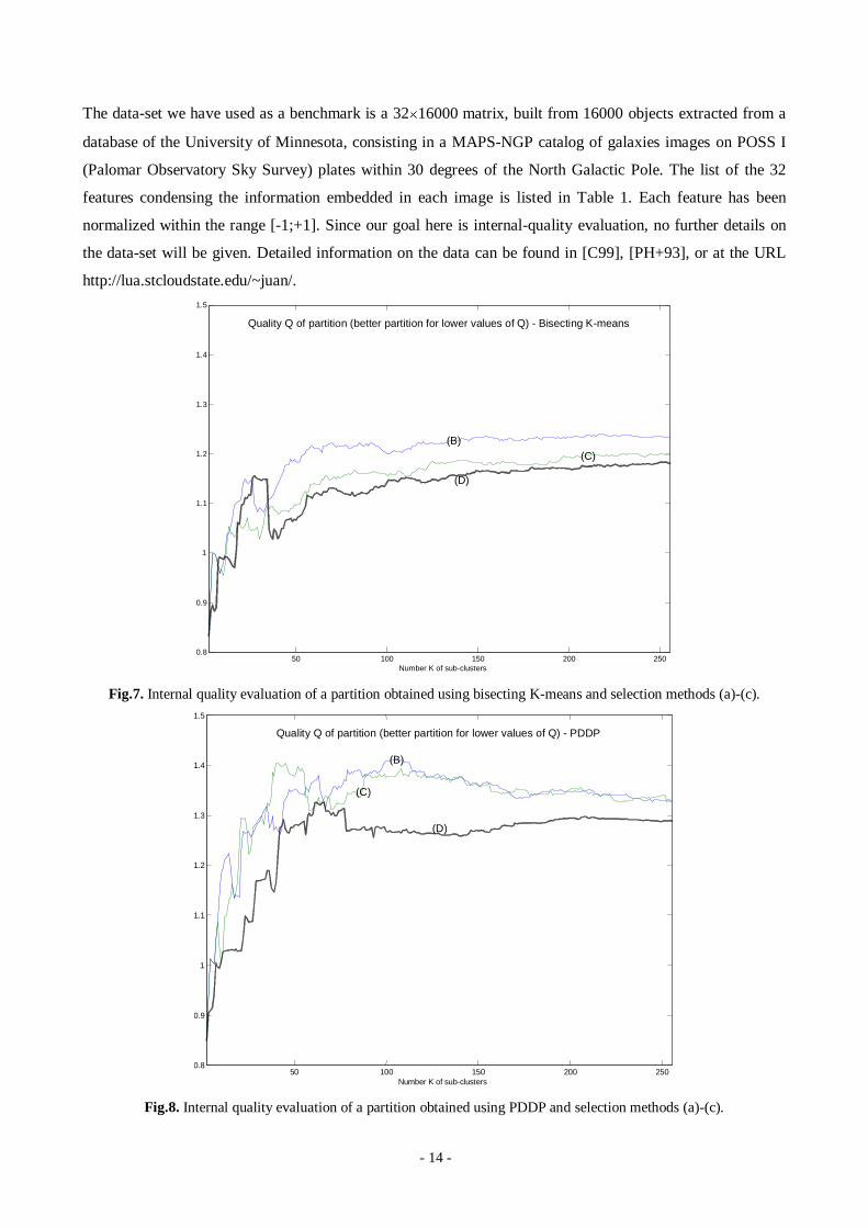
Fig.8. Internal quality evaluation of a partition obtained using PDDP and selection methods (a)-(c).

- 15 -

Using the above 32u16000 matrix, three clustering experiments have been done, both for K-means and

PDDP. The three experiments only differ on the method used for the selection of the cluster to spli t, namely

(see Subsection 3.1):

Method (B): the cluster characterized by the largest number of elements is split;

Method (C): the cluster characterized by the largest scatter is spli t;

Method (D): the cluster characterized by the lowest value of J (see (4)) is spli t, within the set of the 10

clusters having the largest number of elements.

The clustering procedure has been applied iteratively, and stopped when the number of 256 sub-clusters has

been reached. After each step, the quality of the partition has been evaluated using (10). The results are

displayed in Fig. 7 (partition made using bisecting K-means) and in Fig.8 (partition made using PDDP).

By inspecting the results displayed in Figs.7-8, the following can be said:

x Both for K-means and PDDP spli tting algorithms, the method (D) for cluster selection outperforms the

traditional methods (B) and (C). The worst performance is, in both cases, achieved by method (B).

x PDDP seems to take more advantages by method (D) than K-means. Probably this is due to the fact that,

on this particular set of data, K-means provides better performance than PDDP. The possible

improvements hence are more limited.

Even if these results refer to a specific set of data, they are expected to be quite general, since an internal

quality of index has been used. Internal indices are known to be much less application-sensitive than external

indices. The cluster selection based upon )(MJ hence seems to be an effective method to improve the

performance of bisecting divisive clustering algorithms.

5. Conclusions

In this paper the problem of clustering a data-set is considered, using the bisecting divisive partitioning

approach. This approach can be naturally divided into two sub-problems: the problem of choosing which

cluster must be divided, and the problem of spli tting the selected cluster. The focus here is on the first

problem. A new simple technique for the selection of the cluster to spli t has been proposed, which is based

upon the shape of the cluster. This result is presented with reference to two specific splitting algorithms: the

celebrated bisecting K-means algorithm, and the recently proposed Principal Direction Divisive Partitioning

(PDDP) algorithm. The problem of evaluating the clustering performance has been discussed, and a test on a

set of real data has been done.

Acknowledgements

Paper supported by Consiglio Nazionale delle Ricerche (CNR) short-term-mobilit y program, and by NSF

grant IIS-9811229.

- 16 -

References

[A54] Anderson, T. (1954). “On estimation of parameters in latent structure analysis” . Psychometrica, vol.19, pp.1-10.

[BDO95] Berry M.W., S.T. Dumais, G.W. O'Brien (1995). “Using Linear Algebra for intelligent informationretrieval” . SIAM Review, vol.37, pp.573-595.

[BDJ99] Berry, M.W., Z. Drmac, E.R. Jessup (1999). “Matrices, Vector spaces, and Information Retrieval” . SIAMReview, vol.41, pp.335-362.

[B97] Boley, D.L. (1997). “Principal Direction Divisive Partitioning” . Technical Report TR-97-056, Dept. ofComputer Science, University of Minnesota, Minneapolis.

[B98] Boley, D.L. (1998). “Principal Direction Divisive Partitioning” . Data Mining and Knowledge Discovery,vol.2, n.4, pp. 325-344.

[BG+00a] Boley, D.L., M. Gini, R. Gross, S. Han, K. Hastings, G. Karypis, V. Kumar, B. Mobasher, J. Moore (2000).“Partitioning-Based Clustering for Web Document Categorization” . Decision Support Systems (to appear).

[BG+00b] Boley, D.L., M. Gini, R. Gross, S. Han, K. Hastings, G. Karypis, V. Kumar, B. Mobasher, J. Moore (2000).“Document Categorization and Query Generation on the World Wide Web Using WebACE” . AI Review (toappear).

[C99] Cabanela J.E. (1999). Galaxy Properties from a Diameter-limited Catalog. Ph.D. Thesis, University ofMinnesota, MN.

[CY95] Chute, C., Y. Yang (1995). “An overview of statistical methods for the classification and retrieval of patientevents”. Meth. Inform. Med., vol.34, pp.104-110.

[DD+90] Deerwester, S., S. Dumais, G. Furnas, R. Harshman (1990). “ Indexing by latent semantic analysis” . J. Amer.Soc. Inform. Sci, vol.41, pp.41-50.

[F65] Forgy, E. (1965). “Cluster Analysis of Multi variate Data: Eff iciency versus Interpretabil ity ofClassification”. Biometrics, pp.768-780.

[GV96] Golub, G.H, C.F. van Loan (1996). Matrix Computations (3rd edition). The Johns Hopkins University Press.

[GJJ96] Gose, E., R. Johnsonbaugh, S. Jost (1996). Pattern Recognition & Image Analysis. Prentice-Hall .

[JD88] Jain, A.K., R.C. Dubes (1988). Algorithms for clustering data. Prentice-Hall advance reference series.Prentice-Hall , Upper Saddle River, NJ.

[JMF99] Jain, A.K, M.N. Murty, P.J. Flynn (1999). “Data Clustering: a Review” . ACM Computing Surveys, Vol.31,n.3, pp.264-323.

[L50] Lanczos, C. (1950). “An iteration method for the solution of the eigenvalue problem of linear differential andintegral operators” . J. Res. Nat. Bur. Stand, vol.45, pp.255-282.

[L86] LaSalle, J.P. (1986). The Stability and Control of Discrete Processes. Springer-Verlag.

[PH+93] Pennington, R.L., R.M. Humphreys, S.C. Odewahn, W. Zumach, P.M. Thurnes (1993). "The AutomatedPlate Scanner Catalog of The Palomar Sky Survey - Scannig Parameters and Procedures". P.A.S.P, n.105,pp.521-ff.

[S00] Savaresi, S.M. (2000). Data Mining: Algorithms and Applications. Laurea Thesis, Università del SacroCuore, Brescia (in Italian).

[SB00] Savaresi, S.M., D.L. Boley (2000). “Bisecting K-means and PDDP: a comparative analysis” . Submitted.

[SI84] Selim, S.Z., M.A. Ismail (1984). “K-means-type algorithms: a generalized convergence theorem andcharacterization of local optimality” . IEEE Trans. on Pattern Analysis and Machine Intelligence, vol.6, n.1,pp.81-86.

[SKV00] Steinbach, M., G. Karypis, V. Kumar (2000). “A comparison of Document Clustering Techniques” .Proceedings of World Text Mining Conference, KDD2000, Boston.

[V93] Vidyasagar, M. (1993). Nonlinear Systems Analysis. Prentice-Hall

[WW+97] Wang, J.Z., G. Wiederhold, O. Firschein, S.X. Wei (1997). “Content-based image indexing and searchingusing Daubechies' wavelets” . Int. J. Digit. Library, vol.1, pp.311-328.