1

On the performance of bisectingK-means and PDDP *

Sergio M. Savaresi † and Daniel L. Boley ‡

1 Introduction and problem statement

The problem this paper focuses on is the unsupervised clustering of a data-set. The data-set is given by the matrix [ ] Np

NxxxM ×ℜ∈= ,...,, 21 , where each column of M, pix ℜ∈ ,

is a single data-point. This is one of the more basic and common problems in fields likepattern analysis, data mining, document retrieval, image segmentation, decision making,etc. ([12, 13]). The specific problem we want to solve herein is the partition of M into twosub-matrices (or sub-clusters) LNp

LM ×ℜ∈ and RNpRM ×ℜ∈ , NNN RL =+ . This

problem is known as bisecting divisive clustering.Note that by recursively using a divisive bisecting clustering procedure, the data-

set can be partitioned into any given number of clusters. Interestingly enough, the clustersso-obtained are structured as a hierarchical binary tree (or a binary taxonomy). This is thereason why the bisecting divisive approach is very attractive in many applications (e.g. indocument-retrieval/indexing problems – see e.g. [17] and references cited therein).

Among the divisive clustering algorithms which have been proposed in theliterature in the last two decades ([13]), in this paper we will focus on two techniques:• the bisecting K-means algorithm;• the Principal Direction Divisive Partitioning (PDDP) algorithm. * First author supported by Consiglio Nazionale delle Ricerche (CNR) short-term-mobility program. Second author supported by NSF grant IIS-9811229. Thanks are alsodue to Prof. Gene Golub of Dept. of Computer Science at Stanford, to Prof. SergioBittanti of Politecnico di Milano, and to Prof. Giovanna Gazzaniga of Pavia CNRInstitute of Numerical Analysis.

† Dipartimento di Elettronica e Informazione, Politecnico di Milano, Piazza L. da Vinci,32, 20133, Milan, ITALY, savaresi@elet.polimi.it.‡ Department of Computer Science and Engineering, University of Minnesota, 4-192EE/CSci, 200 Union St SE, Minneapolis, MN 55455, USA, boley@cs.umn.edu.

2

K-means is probably the most celebrated and widely used clustering technique;hence it is the best representative of the class of iterative centroid-based divisivealgorithms. On the other hand, PDDP is a recently proposed technique ([4-7]). It isrepresentative of the non-iterative techniques based upon the Singular ValueDecomposition (SVD) of a matrix built from the data-set.

The objective of this paper is twofold:• compare the clustering performance of bisecting K-means and PDDP;• analyze the dynamic behavior of the K-means iterative algorithm.

In the existing literature, both these issues have been considered only empirically.The performance of PDDP and K-means have been recently studied, and have beenreported to be somehow similar, on the basis of a few application examples ([4-7]). Asfor K-means behavior, the main theoretical result known so far is [16], where it is shownthat the K-means iterative procedure is guaranteed to converge; however, nothing is saidabout “where” and “how” it converges.

The main contribution of this work is to provide a simple mathematicalexplanation of some features of K-means and PDDP. This is done under the restrictiveassumption that the data are uniformly distributed within a 2-dimensional ellipsoid. Themain results here obtained can be summarized as follows:• when the number of data-points tends to infinity, K-means and PDDP converge to

the same solution;• when the number of data-points tends to infinity, the iterative bisecting K-means

algorithm is characterized by 2 stationary-points: one is an unstable equilibrium, oneis a stable equilibrium point;

The paper is organized as follows: in Section 2 K-means and PDDP are conciselyrecalled and discussed; in Section 3 they are analyzed when the number of data-pointstends to infinity, whereas in Section 4 an empirical analysis in the case of finite data setsis proposed. Some concluding remarks end the paper.

2 Bisecting K-means and PDDP

As already stated in the Introduction, this paper focuses on two bisecting divisivepartitioning algorithms, which belong to different classes of methods: K-means is themost popular iterative centroid-based divisive algorithm; PDDP is the latest developmentof SVD-based partitioning techniques. The specific algorithms considered herein are nowrecalled and briefly commented. In such algorithms the definition of centroid will be usedextensively; specifically, the centroid of M, say w , is given by

∑=

=N

jjM

Nw

1

1 , (1)

where jM is the j-th columns of M . Similarly, the centroids of the sub-clusters LM and

RM , say Lw and Rw , are given by:

∑∑==

==RL N

jjR

RR

N

jjL

LL M

NwM

Nw

1,

1,

11 , (2)

where jLM , and jRM , are the j-th columns of LM and RM , respectively.

3

Bisecting K-means.Step 1. (Initialization). Randomly select a point, say p

Lc ℜ∈ ; then compute the

centroid w of M (see (1)), and compute pRc ℜ∈ as )( wcwc LR −−= .

Step 2. Divide [ ]NxxxM ,...,, 21= into two sub-clusters LM and RM , according to thefollowing rule:

−>−∈

−≤−∈

RiLiRi

RiLiLi

cxcxifMx

cxcxifMx

Step 3. Compute the centroids of LM and RM , Lw and Rw , as in (2).Step 4. If LL cw = and RR cw = , stop, else, let LL wc = , RR wc = and go to Step 2.

The algorithm above presented is the bisecting version of the general K-meansalgorithm. This bisecting algorithm has been recently discussed and emphasized in [17]and [19]. In these works it is claimed to be very effective in document-processingproblems. It is here worth noting that the algorithm above recalled is the very classicaland basic version of K-means, also known (see [10, 12]) as Forgy’s algorithm (with aslight modification of the initialization step). Many variations of this basic version of thealgorithm have been proposed, aiming to reduce the computational demand, at the priceof (hopefully little) sub-optimality. Since the goal of this paper is to analyze convergenceproperties and clustering performance, this original version of the K-means algorithm isthe most interesting and meaningful.

PDDPStep 1. Compute the centroid w of M as in (1).Step 2. Compute the auxiliary matrix M~ as weMM −=~ , where e is a N-dimensionalrow vector of ones, namely [ ]1,...1,1,1,1,1=e .Step 3. Compute the Singular Value Decompositions (SVD) of M~ , TVUM Σ=~ ,where Σ is a diagonal Np × matrix, and U and V are ortonormal unitary square matriceshaving dimension pp × and NN × , respectively (see [11] for an exhaustive descriptionof SVD).Step 4. Take the first column vector of U, say 1Uu = , and divide [ ]NxxxM ,...,, 21=into two sub-clusters LM and RM , according to the following rule:

>−∈

≤−∈

0)(

0)(

wxuifMx

wxuifMx

iT

Ri

iT

Li .

The PDDP algorithm, recently proposed in [5], belongs to the class of SVD-baseddata-processing algorithms ([2, 3]); among them, the most popular and widely known arethe Latent Semantic Indexing algorithm (LSI – see [1, 9]), and the LSI-related LinearLeast Square Fit (LLSF) algorithm ([8]). PDDP and LSI mainly differ in the fact that thePDDP splits the matrix with hyperplane passing through its centroid; LSI through theorigin. Another major feature of PDDP is that the SVD of M~ (Step 3.) can be stopped atthe first singular value/vector. This makes PDDP significantly less computationallydemanding than LSI, especially if the data-matrix is sparse and the principal singularvector is calculated by resorting to the Lanczos technique ( [11, 14]).

4

-1 -0.5 0 0.5 1 1.5

-1

-0.5

0

0.5

1

1.5 Bisecting K-means partition

-1 -0.5 0 0.5 1 1.5

-1

-0.5

0

0.5

1

1.5 PDDP partition

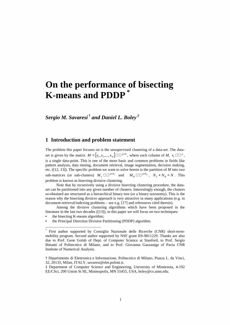
Fig.1a. Partitioning line (bold) ofbisecting K-means algorithm. The bulletsare the centroids of the data-set and of thetwo sub-clusters.

Fig.1b. Partitioning line (bold) of PDDPalgorithm. The bullet is the centroid of thedata set. The two arrows show theprincipal direction of M~ .

The main difference between K-means and PDDP is that K-means is based uponan iterative procedure, which, in general, provides different results for differentinitializations, whereas PDDP is a “one-shot” algorithm, which provides a uniquesolution. In order to understand better how K-means and PDDP work, in Fig.1a andFig.1b the partition of a generic matrix of dimension 20002× provided by K-means andPDDP, respectively, is displayed. From Fig.1, it is easy to see how K-means and PDDPwork:• the bisecting K-means algorithm splits M with an hyperplane which passes through

the centroid w of M, and is perpendicular to the line passing through the centroidsLw and Rw of the sub-clusters LM and RM . This is due to the fact that the stopping

condition for K-means iterations is that each element of a cluster must be closer tothe centroid of that cluster than the centroid of any other cluster.

• PDDP splits M with an hyperplane which passes through the centroid w of M, and isperpendicular to the principal direction of the “unbiased” matrix M~ (note that M~ isthe translated version of M, having the origin as centroid). The principal direction ofM~ is its direction of maximum variance (see [11]).

At a first glance, the two clusters provided by K-means and PDDP look almostindistinguishable. A more careful analysis reveals that the two partitions differ by a fewpoints. Note that this is somewhat unexpected, since the two algorithms differsubstantially.

In the rest of the paper we will try to give a rational explanation to the fact thatPDDP and bisecting K-means may provide similar results. This will be done by analyzingthe dynamic behavior of K-means iteration. Moreover, we will try to clearly outline thepros and cons of these two seemingly equivalent algorithms.

The analysis presented in the following two sections is based upon the restrictiveassumption that the points of the data-set are uniformly distributed within an ellipsoid.This assumption deserves some comments:

5

It is important pointing out that an answer to the question “where does K-meansconverge?” can be found only if an assumption of the data-distribution is made. Note thatthis is not mandatory if one only wants an answer to the question “does the K-meansiteration converge?” (as a matter of fact in [16] no assumptions on the data distributionare made). Therefore, the sensible choice of the data distribution becomes the main issue.

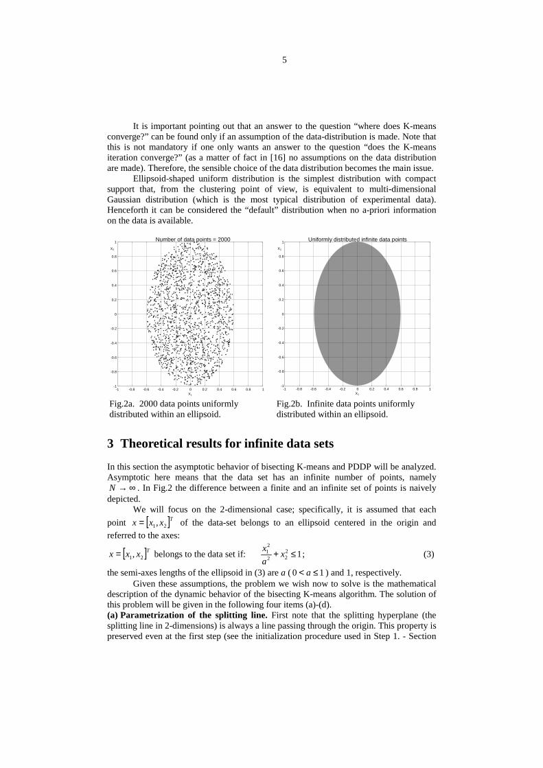
Ellipsoid-shaped uniform distribution is the simplest distribution with compactsupport that, from the clustering point of view, is equivalent to multi-dimensionalGaussian distribution (which is the most typical distribution of experimental data).Henceforth it can be considered the “default” distribution when no a-priori informationon the data is available.

-1 -0.8 -0.6 -0.4 -0.2 0 0.2 0.4 0.6 0.8 1-1

-0.8

-0.6

-0.4

-0.2

0

0.2

0.4

0.6

0.8

1

X1

X2

Number of data points = 2000

-1 -0.8 -0.6 -0.4 -0.2 0 0.2 0.4 0.6 0.8 1-1

-0.8

-0.6

-0.4

-0.2

0

0.2

0.4

0.6

0.8

1

X1

X2

Uniformly distributed infinite data points

Fig.2a. 2000 data points uniformlydistributed within an ellipsoid.

Fig.2b. Infinite data points uniformlydistributed within an ellipsoid.

3 Theoretical results for infinite data sets

In this section the asymptotic behavior of bisecting K-means and PDDP will be analyzed.Asymptotic here means that the data set has an infinite number of points, namely

∞→N . In Fig.2 the difference between a finite and an infinite set of points is naivelydepicted.

We will focus on the 2-dimensional case; specifically, it is assumed that eachpoint [ ]Txxx 21,= of the data-set belongs to an ellipsoid centered in the origin andreferred to the axes:

[ ]Txxx 21,= belongs to the data set if: 1222

21 ≤+ x

ax ; (3)

the semi-axes lengths of the ellipsoid in (3) are a ( 10 ≤< a ) and 1, respectively.Given these assumptions, the problem we wish now to solve is the mathematical

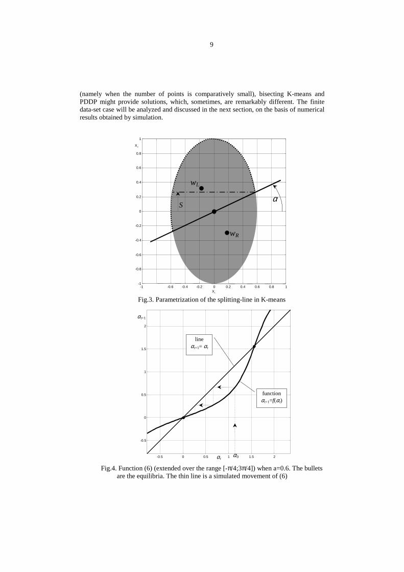
description of the dynamic behavior of the bisecting K-means algorithm. The solution ofthis problem will be given in the following four items (a)-(d).(a) Parametrization of the splitting line. First note that the splitting hyperplane (thesplitting line in 2-dimensions) is always a line passing through the origin. This property ispreserved even at the first step (see the initialization procedure used in Step 1. - Section

6

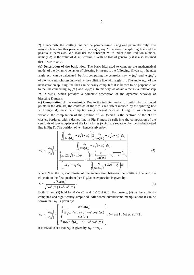
2). Henceforth, the splitting line can be parameterized using one parameter only. Thenatural choice for this parameter is the angle, say α, between the splitting line and thepositive x1 semi-axis. We shall use the subscript “t” to indicate the iteration number,namely tα is the value of α at iteration t. With no loss of generality it is also assumedthat 2/0 πα ≤≤ t .(b) Description of the basic idea. The basic idea used to compute the mathematicalmodel of the dynamic behavior of bisecting K-means is the following. Given tα , the nextangle 1+tα can be calculated by first computing the centroids, say )( tLw α and )( tRw α ,of the two semi-clusters induced by the splitting line with angle tα . The angle 1+tα of thenext-iteration splitting line then can be easily computed: it is known to be perpendicularto the line connecting )( tLw α and )( tRw α . In this way we obtain a recursive relationship

)(1 tt f αα =+ , which provides a complete description of the dynamic behavior ofbisecting K-means.(c) Computation of the centroids. Due to the infinite number of uniformly distributedpoints in the data-set, the centroids of the two sub-clusters induced by the splitting linewith angle tα must be computed using integral calculus. Using 2x as integrationvariable, the computation of the position of Lw (which is the centroid of the “Left”cluster, bordered with a dashed line in Fig.3) must be split into the computation of thecentroids of two sub-pieces of the Left cluster (which are separated by the dashed-dottedline in Fig.3). The position of Lw hence is given by:

−+

−+⋅

+−

−⋅

−+

−+⋅

−−

=

=

∫

∫

∫

∫

∫

∫

−

−

−

−

−

−

S

S t

S

S tS

S

S

S

S

S t

S

S tt

L

LL

dxxax

dxxaxx

dxxa

dxxax

dxxax

dxxaxxax

ww

w

222

2

222

22

222

2222

222

2

222

222

2

2

1

1)tan(

1)tan(

12

12

1)tan(

1)tan(

1)tan(

α

α

α

αα

, (4)

where S is the 2x -coordinate of the intersection between the splitting line and theellipsoid in the first quadrant (see Fig.3); its expression is given by:

)()(cos

)(222

tt

t

sina

sinaSαα

α+

⋅= . (5)

Both (4) and (5) hold for 10 ≤< a and 2/0 πα ≤≤ t . Fortunately, (4) can be explicitlycomputed and significantly simplified. After some cumbersome manipulations it can beshown that Lw is given by:

−+

−+−

=

=

)(cos)(cos

)cos(34

)(cos)(cos

)(34

2222

2222

2

2

1

tt

t

tt

t

L

LL

aa

aa

sina

ww

w

ααπα

ααπα

, 10 ≤< a , 2/0 πα ≤≤ t ;

it is trivial to see that Rw is given by LR ww −= .

7

(d) The dynamic model of bisecting K-means. Once )( tLw α and )( tRw α have beenfound, it is easy to compute the recursive function )(1 tt f αα =+ which models thetransition from tα to the angle 1+tα of the next-iteration splitting line. Indeed, this linemust be perpendicular to the line passing through Lw and Rw , namely:

=+1tα atan [ ])tan(2ta α , 10 ≤< a , 2/0 πα ≤≤ t . (6)

Equation (6) is one of the major results of this work, since it provides a rigorousclosed-form explicit expression of the dynamic behavior of bisecting K-means in thelimiting case. Note that (6) represents a first order autonomous (i.e. without forcinginputs) non-linear dynamic discrete-time system. As such, it can be analyzed using non-linear systems theory (see e.g. [15, 18]). The analysis of (6) reveals that:• By solving the steady-state equation =α atan [ ])tan(2 αa , it is easy to see that the

iterative K-means procedure can only have two stationary-points, at 0=α and2/πα = . In correspondence to these points the ellipsoid is divided by its shorter

axis ( 0=α ), and by its longer axis ( 2/πα = ), respectively.• By locally linearizing the dynamic system (6) about the admissible equilibrium

points (namely by computing the tangent model ( )( ) ttttt

f δαααδα αα =+ ∂∂= )(1 ,

where ααδα −= tt : ), we obtain the following two linear dynamic discrete-timesystems:

local dynamic behavior about 0=α : tt a δαδα )( 21 =+ , 0: −= tt αδα ;

local dynamic behavior about 2/πα = : tt a δαδα )/1( 21 =+ , 2/: παδα −= tt .

From linear discrete-time dynamic system theory we know that, if 10 << a , thelinear system about 0=α is asymptotically stable, and the linear system about

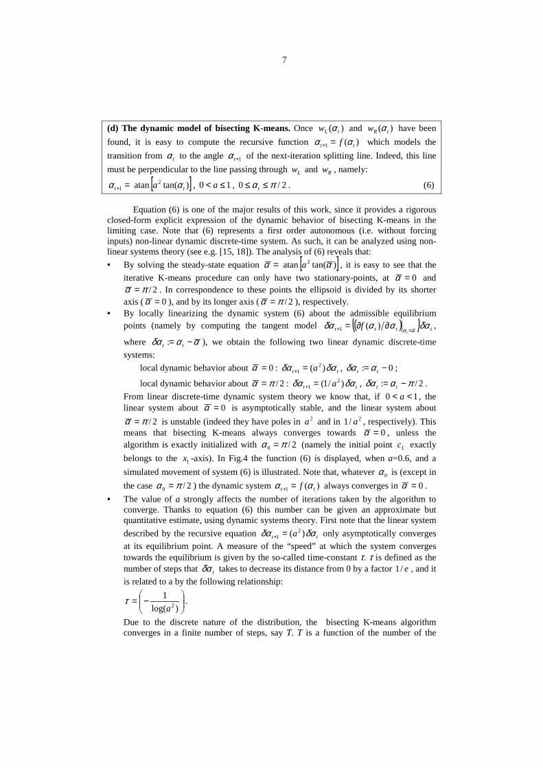
2/πα = is unstable (indeed they have poles in 2a and in 2/1 a , respectively). Thismeans that bisecting K-means always converges towards 0=α , unless thealgorithm is exactly initialized with 2/0 πα = (namely the initial point Lc exactlybelongs to the 1x -axis). In Fig.4 the function (6) is displayed, when a=0.6, and asimulated movement of system (6) is illustrated. Note that, whatever 0α is (except inthe case 2/0 πα = ) the dynamic system )(1 tt f αα =+ always converges in 0=α .

• The value of a strongly affects the number of iterations taken by the algorithm toconverge. Thanks to equation (6) this number can be given an approximate butquantitative estimate, using dynamic systems theory. First note that the linear systemdescribed by the recursive equation tt a δαδα )( 2

1 =+ only asymptotically convergesat its equilibrium point. A measure of the “speed” at which the system convergestowards the equilibrium is given by the so-called time-constant τ. τ is defined as thenumber of steps that tδα takes to decrease its distance from 0 by a factor e/1 , and itis related to a by the following relationship:

−=

)log(1

2aτ .

Due to the discrete nature of the distribution, the bisecting K-means algorithmconverges in a finite number of steps, say T. T is a function of the number of the

8

data-points N (namely it depends on how densely the data are distributed), which isexpected to be proportional to τ, namely:

−⋅=

)log(1)( 2a

NT γ . (7)

The exact value of )(Nγ is hard to be predicted exactly. A rule-of-thumb typicallyused by the control systems practitioner can be used to have an idea of )(Nγ : thisrule says that, when tδα has reached the 98% of the distance between the initialvalue and the equilibrium, the system can be considered, in practice, at steady-state.It is easy to see that this corresponds to 4)( ≈Nγ . In Section 4 a numericalvalidation of this formula will be provided.Finally note that T may take very different values. For instance (if 4)( ≈Nγ ), K-means is expected to take only 10-15 iterations to converge if a=0.7, about 40iterations are needed if a=0.9, whereas if a=0.95 the algorithm might need 80iterations to converge. It is important to observe, however, that (7) is expected toprovide a reliable estimate of T only if the number of the points of the data-set islarge. For small data-sets the number of iterations required by K-means can beconsiderably smaller than (7).

The analysis above presented is the main contribution of this Section. It can beconcisely summarized with the following two propositions.

Proposition 1. If the data-points of a data-set are uniformly distributed in a 2-dimensional ellipsoid, the semi-axes of the hyper-ellipsoid have lengths equal to 1 and a,(0<a<1), and ∞→N , then the dynamic discrete-time system which models the K-meansiterative algorithm is characterized by 2 equilibrium points; one is locally unstable, andone is locally stable. In particular, the dynamic model has the form:

=+1tα atan ))tan(( 2ta α , 2/0 πα ≤≤ t . The splitting hyperplanes corresponding to the

equilibrium points pass through the origin and are orthogonal to the main axes of theellipsoid. The splitting hyperplane corresponding to the stable equilibrium point isorthogonal to the largest axis of the ellipsoid.Proof. The proof of this result is given in items (a)-(d) above. !

Proposition 2. If the data-points of a data-set are uniformly distributed in a 2-dimensional ellipsoid, the semi-axes of the hyper-ellipsoid have lengths equal to 1 and a,(0<a<1), and ∞→N , then the PDDP algorithm splits the ellipsoid with an hyperplanepassing through the origin and orthogonal to the largest axis of the ellipsoid.Proof. This result is a direct implication of the properties of the SVD. Indeed the 2singular vectors of a set of points uniformly distributed within an ellipsoid coincide withthe direction of the principal axes of the ellipsoid (see [11] for details).

!

Propositions 1 and 2 show that bisecting K-means and PDDP provide the samesolution, except in the case when the initialization of K-means exactly corresponds to anunstable equilibrium point of the K-means dynamic model. However, if the initializationis made randomly, this event occurs with probability zero.

These asymptotic results are useful to gain a deep insight into the bisecting K-means algorithm, and to explain why, in many cases, K-means and PDDP show a verysimilar clustering behavior. However, when the data set contains a finite number of data

9

(namely when the number of points is comparatively small), bisecting K-means andPDDP might provide solutions, which, sometimes, are remarkably different. The finitedata-set case will be analyzed and discussed in the next section, on the basis of numericalresults obtained by simulation.

-1 -0.6 -0.4 -0.2 0 0.2 0.4 0.6 0.8 1-1

-0.8

-0.6

-0.4

-0.2

0

0.2

0.4

0.6

0.8

1

X1

X2

α

wR

S

wL

Fig.3. Parametrization of the splitting-line in K-means

-0.5 0 0.5 1 1.5 2

-0.5

0

0.5

1

1.5

2

α t

αt+1

α0

lineα t+1= αt

functionαt+1=f(αt)

Fig.4. Function (6) (extended over the range [-π/4;3π/4]) when a=0.6. The bulletsare the equilibria. The thin line is a simulated movement of (6)

10

4 Numerical results for finite data sets

In this section, the bisecting K-means and PDDP will be analyzed when the data-set has a finite number of data-points. The analysis will be done empirically, usingsimulated data.

The purpose of this section is twofold:• validate the theoretical results obtained in the previous section, and see how they

change when the data-set is finite;• understand the pros and cons of K-means and PDDP.

The analysis is structured as follows: first the dynamic model of K-means will benumerically computed for finite data-sets, and the problem of local minima will bediscussed; then the formula (7) for the estimation of the number of iterations required byK-means to converge will be validated.

-0.5 0 0.5 1 1.5 2

-0.5

0

0.5

1

1.5

2

α(t+1)

Number of data points = 15; a=0.6

(a)

Equilibriumpoints

α(t) -0.5 0 0.5 1 1.5 2

-0.5

0

0.5

1

1.5

2

Number of data points = 30; a=0.6

(b)α(t+1)

α(t)

-0.5 0 0.5 1 1.5 2

-0.5

0

0.5

1

1.5

2

Number of data points = 100; a=0.6

(c)α(t+1)

α(t) -0.5 0 0.5 1 1.5 2

-0.5

0

0.5

1

1.5

2

Number of data points = 2000; a=0.6

(d)α(t+1)

α(t)

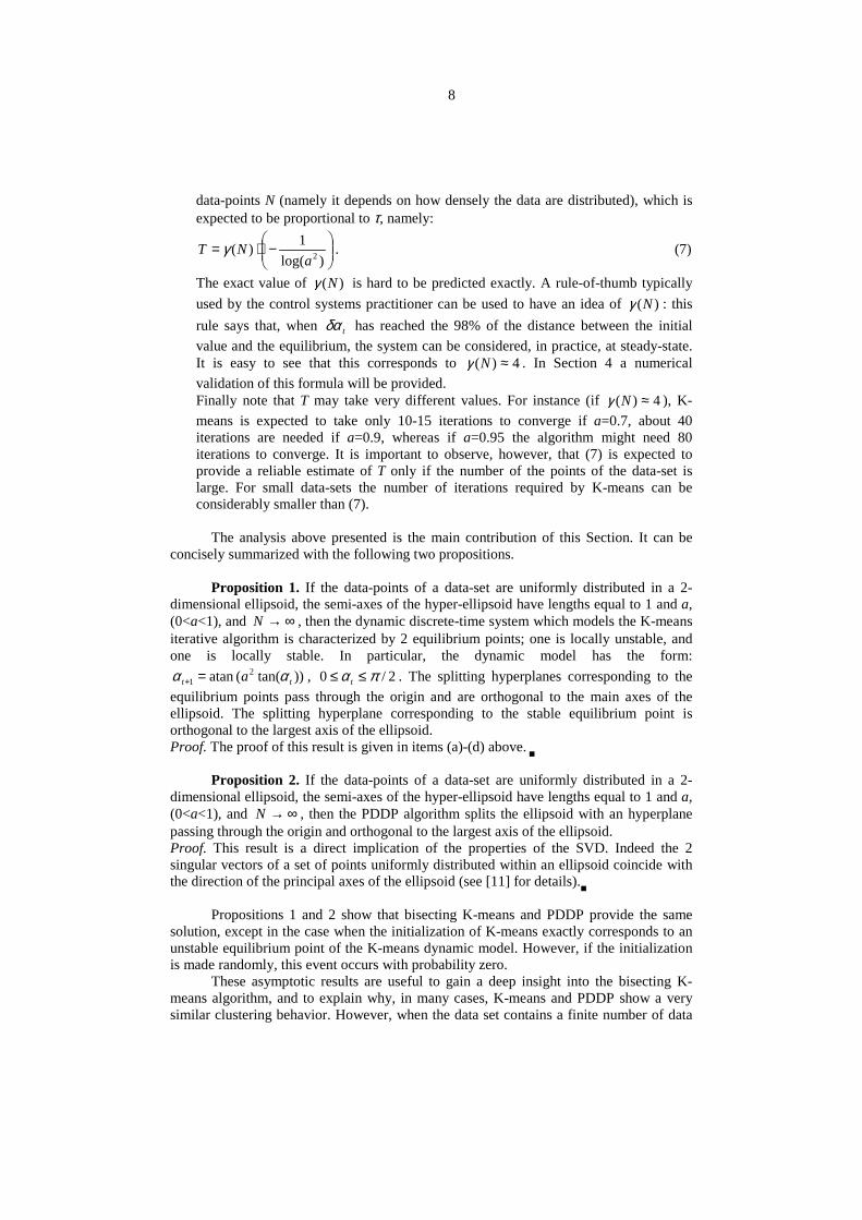
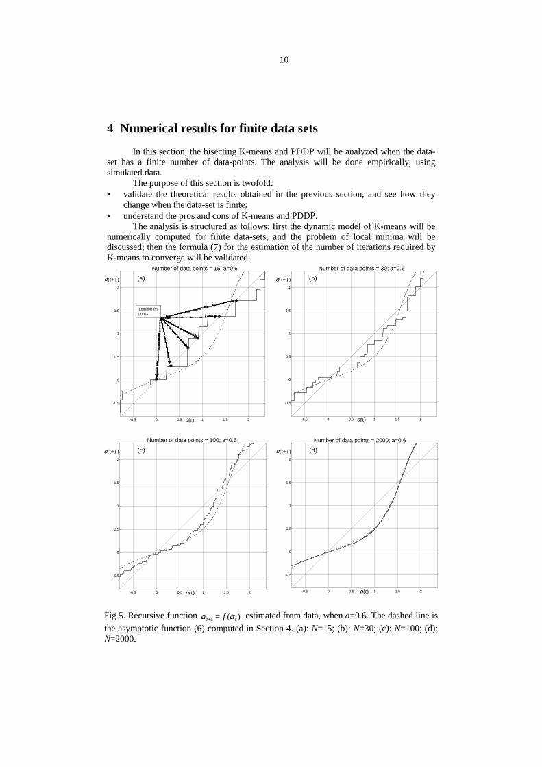
Fig.5. Recursive function )(1 tt f αα =+ estimated from data, when a=0.6. The dashed line isthe asymptotic function (6) computed in Section 4. (a): N=15; (b): N=30; (c): N=100; (d):N=2000.

11

The first problem we consider is the analysis of the K-means dynamic behaviorwhen the data-set has a finite number of data. As a first experiment, four sets of data havebeen considered, characterized by 15, 30, 100 and 2000 data-points uniformly distributedwithin a 2-dimensional ellipsoid with a=0.6. The recursive function )(1 tt f αα =+ hasbeen numerically computed for these four data-sets. The results are displayed in Fig.5.From the inspection of Fig.5, the following remarks can be done:

The main difference between the asymptotic function (6) and the recursivefunctions corresponding to finite data-sets is that the latter are step-wise functions. Amajor consequence of this function being step-like is that every equilibrium point(namely every point where the function crosses the line tt αα =+1 - see Fig.5a) is locallyasymptotically stable, since the local slope of the function about the equilibrium issmaller than 1. Note that this explains why K-means is affected by “local minima”problems.

-0.5 0 0.5 1 1.5 2

-0.5

0

0.5

1

1.5

2

Number of data points = 15; a=0.9

(a)α(t+1)

α(t)-0.5 0 0.5 1 1.5 2

-0.5

0

0.5

1

1.5

2

Number of data points = 30; a=0.9

(b)α(t+1)

α(t)

-0.5 0 0.5 1 1.5 2

-0.5

0

0.5

1

1.5

2

Number of data points = 100; a=0.9

(c)α(t+1)

α(t)-0.5 0 0.5 1 1.5 2

-0.5

0

0.5

1

1.5

2

Number of data points = 2000; a=0.9

(d)α(t+1)

α(t)

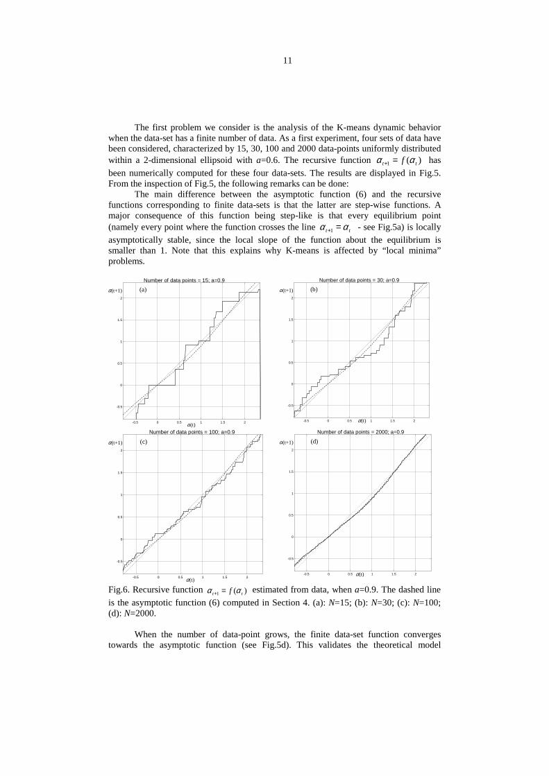
Fig.6. Recursive function )(1 tt f αα =+ estimated from data, when a=0.9. The dashed lineis the asymptotic function (6) computed in Section 4. (a): N=15; (b): N=30; (c): N=100;(d): N=2000.

When the number of data-point grows, the finite data-set function convergestowards the asymptotic function (see Fig.5d). This validates the theoretical model

12

developed in the previous section. Moreover, notice that when the number of data-pointgets large, the number of equilibrium points decreases, and each step gets narrower (seee.g. Fig.5c). This explains why, when the number of data is sufficiently large, it is thecommon experience that the problem of local minima tends to vanish.

As a second experiment, the recursive function )(1 tt f αα =+ has been computedfor four sets of 15, 30, 100 and 2000 data-points uniformly distributed within a 2-dimensional ellipsoid with a=0.9. The results are displayed in Fig.6. The main differencein the results between the case a=0.6 and a=0.9 is that in the latter the problem ofmultiple equilibrium points is more severe.

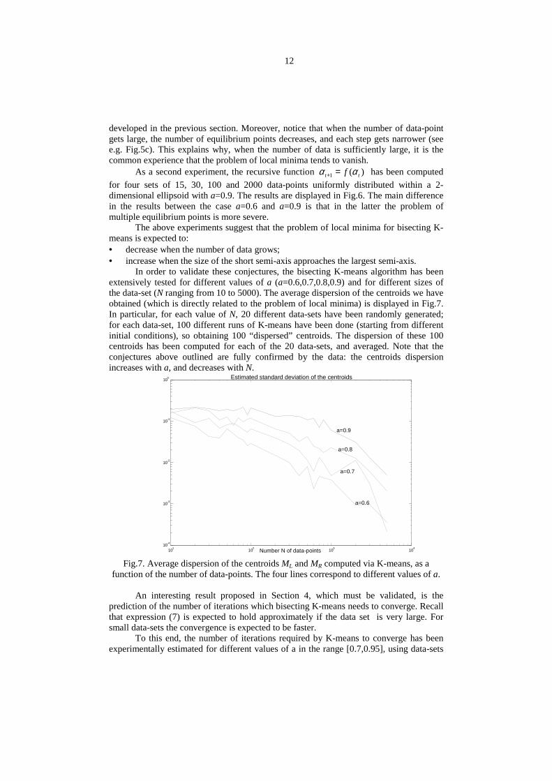
The above experiments suggest that the problem of local minima for bisecting K-means is expected to:• decrease when the number of data grows;• increase when the size of the short semi-axis approaches the largest semi-axis.

In order to validate these conjectures, the bisecting K-means algorithm has beenextensively tested for different values of a (a=0.6,0.7,0.8,0.9) and for different sizes ofthe data-set (N ranging from 10 to 5000). The average dispersion of the centroids we haveobtained (which is directly related to the problem of local minima) is displayed in Fig.7.In particular, for each value of N, 20 different data-sets have been randomly generated;for each data-set, 100 different runs of K-means have been done (starting from differentinitial conditions), so obtaining 100 “dispersed” centroids. The dispersion of these 100centroids has been computed for each of the 20 data-sets, and averaged. Note that theconjectures above outlined are fully confirmed by the data: the centroids dispersionincreases with a, and decreases with N.

101

102

103

104

10-4

10-3

10-2

10-1

100

Number N of data-points

Estimated standard deviation of the centroids

a=0.9

a=0.8

a=0.7

a=0.6

Fig.7. Average dispersion of the centroids ML and MR computed via K-means, as afunction of the number of data-points. The four lines correspond to different values of a.

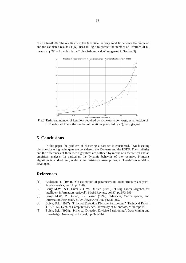
An interesting result proposed in Section 4, which must be validated, is theprediction of the number of iterations which bisecting K-means needs to converge. Recallthat expression (7) is expected to hold approximately if the data set is very large. Forsmall data-sets the convergence is expected to be faster.

To this end, the number of iterations required by K-means to converge has beenexperimentally estimated for different values of a in the range [0.7,0.95], using data-sets

13

of size N=20000. The results are in Fig.8. Notice the very good fit between the predictedand the estimated results ( )(Nγ used in Fig.8 to predict the number of iterations of K-means is 4)( =Nγ , which is the “rule-of-thumb value" suggested in Section 3).

0.7 0.75 0.8 0.85 0.9 0.9510

20

30

40

50

60

70

80

Size of the shorter semi-axis a

Number of steps taken by K-means to converge - Number of data-points = 20000

Fig.8. Estimated number of iterations required by K-means to converge, as a function ofa. The dashed line is the number of iterations predicted by (7), with γ(N)=4.

5 Conclusions

In this paper the problem of clustering a data-set is considered. Two bisectingdivisive clustering techniques are considered: the K-means and the PDDP. The similarityand the differences of these two algorithms are outlined by means of a theoretical and anempirical analysis. In particular, the dynamic behavior of the recursive K-meansalgorithm is studied, and, under some restrictive assumptions, a closed-form model isdeveloped.

References

[1] Anderson, T. (1954). “On estimation of parameters in latent structure analysis”.Psychometrica, vol.19, pp.1-10.

[2] Berry M.W., S.T. Dumais, G.W. O'Brien (1995). “Using Linear Algebra forintelligent information retrieval”. SIAM Review, vol.37, pp.573-595.

[3] Berry, M.W., Z. Drmac, E.R. Jessup (1999). “Matrices, Vector spaces, andInformation Retrieval”. SIAM Review, vol.41, pp.335-362.

[4] Boley, D.L. (1997). “Principal Direction Divisive Partitioning”. Technical ReportTR-97-056, Dept. of Computer Science, University of Minnesota, Minneapolis.

[5] Boley, D.L. (1998). “Principal Direction Divisive Partitioning”. Data Mining andKnowledge Discovery, vol.2, n.4, pp. 325-344.

14

[6] Boley, D.L., M. Gini, R. Gross, S. Han, K. Hastings, G. Karypis, V. Kumar, B.Mobasher, J. Moore (2000). “Partitioning-Based Clustering for Web DocumentCategorization”. Decision Support Systems, Vol.27, n.3, pp.329-341.

[7] Boley, D.L., M. Gini, R. Gross, S. Han, K. Hastings, G. Karypis, V. Kumar, B.Mobasher, J. Moore (2000). “Document Categorization and Query Generation onthe World Wide Web Using WebACE”. AI Review, Vol.13, n.5-6, pp.365-391.

[8] Chute, C., Y. Yang (1995). “An overview of statistical methods for theclassification and retrieval of patient events”. Meth. Inform. Med., vol.34, pp.104-110.

[9] Deerwester, S., S. Dumais, G. Furnas, R. Harshman (1990). “Indexing by latentsemantic analysis”. J. Amer. Soc. Inform. Sci, vol.41, pp.41-50.

[10] Forgy, E. (1965). “Cluster Analysis of Multivariate Data: Efficiency versusInterpretability of Classification”. Biometrics, pp.768-780.

[11] Golub, G.H, C.F. van Loan (1996). Matrix Computations (3rd edition). The JohnsHopkins University Press.

[12] Gose, E., R. Johnsonbaugh, S. Jost (1996). Pattern Recognition & Image Analysis.Prentice-Hall.

[13] Jain, A.K, M.N. Murty, P.J. Flynn (1999). “Data Clustering: a Review”. ACMComputing Surveys, Vol.31, n.3, pp.264-323.

[14] Lanczos, C. (1950). “An iteration method for the solution of the eigenvalueproblem of linear differential and integral operators”. J. Res. Nat. Bur. Stand,vol.45, pp.255-282.

[15] LaSalle, J.P. (1986). The Stability and Control of Discrete Processes. Springer-Verlag.

[16] Selim, S.Z., M.A. Ismail (1984). “K-means-type algorithms: a generalizedconvergence theorem and characterization of local optimality”. IEEE Trans. onPattern Analysis and Machine Intelligence, vol.6, n.1, pp.81-86.

[17] Steinbach, M., G. Karypis, V. Kumar (2000). “A comparison of DocumentClustering Techniques”. Proceedings of World Text Mining Conference,KDD2000, Boston.

[18] Vidyasagar, M. (1993). Nonlinear Systems Analysis. Prentice-Hall[19] Wang, J.Z., G. Wiederhold, O. Firschein, S.X. Wei (1997). “Content-based image

indexing and searching using Daubechies' wavelets”. Int. J. Digit. Library, vol.1,pp.311-328.