Embed Size (px)
Citation preview

CHEE 222: PROCESS DYNAMICS AND NUMERICAL METHODS
Winter 2017
Module 1: Introduction to Process Modeling
Dr. Xiang Li

Module 1 Outline 1. Process and Model - Concepts of process and model - Classification of models and processes - Fundamental model and empirical model - Lumped parameter system and distributed parameter system - Steady-state model and dynamic model
2. Formulating Fundamental Models - Equations physical-chemical relationships - Equations from conservation laws: Material balance, energy balance. - Equations from constitutive relationships
- Model organization - States, inputs, parameters - Dimensionless model - General form of dynamic models – Vector notation
1

Process • A process is any operation or series of operations by which a particular
objective is accomplished (Felder and Rousseau, 2005).
• A chemical process involves transformation of raw materials and input energy into desired products.
Chemical Process Raw Materials
Products
Energy In
Energy Loss
Byproducts/Wastes
1. Process and Model
2

Chemical Process: Fischer-Tropsch Process
Raw Materials: Syngas (CO, H2)
Products: Hydrocarbon fuels
(e.g., Diesel)
Energy (Heat) In
Energy (Heat) Loss
Byproducts/Wastes: Flue gas, sour water
1. Process and Model Fischer–Tropsch process
(2n+1)H2+nCO è CnH(2n+1)+nH2O
3
Operated at 150–300°C and with a high pressure

1. Process and Model
Chemical Process Raw Materials
Products
Energy In
Energy Loss
Byproducts/Wastes
Considerations in Chemical Processing (1) …
!
Desired!process!features! Relevant!physical!quantities!(process!variables)!
High%throughput%(productivity)% Flow%rate,%…%High%product%quality% Concentration,%density,%pH%level…%
Low%energy%consumption% Heat,%temperature,%…%Low%emission%and%effluent% Concentration,%flow%rate,%…%
%Desired process features are achieved via “driving” process variables to appropriate values.
4

Considerations in Chemical Processing (2) …
• Synthesis: What sequence of of units (mixers, heaters, reactors, separators)?
• Design: What type and size of equipment?
• Operation: What operating conditions will optimize product yield?
• Control: How to maintain a measured process variable at a desired value ?
• Safety: What if a process unit fails?
• Environmental: How can we operate the system to minimize pollutants ?
Answer the above questions via trial-and-error? - Expensive, time-consuming, dangerous, limitation of the results …
1. Process and Model
5

Model A mathematical or physical system obeying certain specified conditions, whose behavior is used to understand a physical, biological, or social system to which it is analogous to.
“McGraw-Hill Dictionary of Scientific and Technical Terms”
1. Process and Model
6
Second step – A physical model
Physical aircraft model in wind tunnel (http://www.windtunnels.arc.nasa.gov/pics/12FT/12ft4.html)

Process Model A process model is a set of equations (including necessary input data to solve the equations) that allows us to predict the behavior of a chemical process system.
1. Process and Model
- Bequette, B.W. Process Dynamics: Modeling, Analysis and Simulation, Prentice Hall, Upper Saddle River, NJ (1998)
F1 (L/s) F2 (L/s)
F3 (L/s)
, C1 (mol/L) , C2 (mol/L)
, C3 (mol/L) F1C1 + F2C2 = F3C3
F1 + F2 = F3
With appropriate assumptions, steady-state model of tank inlet/outlet streams
7

Considerations in Chemical Processing (2) …
• Synthesis: What sequence of of units (mixers, heaters, reactors, separators)?
• Design: What type and size of equipment?
• Operation: What operating conditions will optimize product yield?
• Control: How to maintain a measured process variable at a desired value ?
• Safety: What if a process unit fails?
• Environmental: How can we operate the system to minimize pollutants ?
Answer the above questions via trial-and-error? - Expensive, time-consuming, dangerous, limitation of the results …
1. Process and Model
8
Answer the above questions via process models! - Inexpensive (computers, manpower), faster (???), safe, scalability

The Nobel Prize in Chemistry 2013 was awarded jointly to Martin Karplus, Michael Levitt and Arieh Warshel "for the development of multiscale models for complex chemical systems".
From http://www.nobelprize.org/nobel_prizes/chemistry/
9
Mathematical Models and Methods for Chemistry

Understand a Process via Understanding the Model 1. Process and Model • Using process model to simulate/predict process behavior under
different conditions without doing real physical experiments. • For a reliable and effective simulation/prediction, we must ensure
that (1) The process model consists of “correct equations”; (2) We can solve the model (equations) “correctly”.
10

11
Engineers “mirror” processes into models
x = f(x,u,p)
http://www.needlevalve.co.in/images/chemical-plant.jpg
A good model is like …
http://en.wikipedia.org/wiki/Mirror
1. Process and Model
12
x = f(x,u,p)
A poor model is like …
Engineers “mirror” processes into models
http://poojycat.files.wordpress.com/2012/10/p1170732.jpg%3Fw%3D538%26h%3D594
http://www.needlevalve.co.in/images/chemical-plant.jpg
1. Process and Model

13
Perhaps a good model but with incorrect interpretation (solution) …
Engineers “mirror” processes into models
x = f(x,u,p)
http://www.needlevalve.co.in/images/chemical-plant.jpg
http://www.npr.org/blogs/pictureshow/2012/08/07/157743116/does-the-mirror-reflect-how-you-feel
1. Process and Model

Classification of Mathematical Models: Fundamental vs. Empirical
1. Process and Model • Fundamental Model (First-Principle Model)
• These models are based on known physical-chemical relationships • Conservation laws
• Material balance • Energy balance • Momentum balance (CHEE 223)
• Constitutive Relationships • Ideal gas law • Reaction kinetics or rate laws • Heat transfer laws
• Empirical Model (CHEE 209, CHEE 418): • These models are developed directly from measurement/known process
data. • They are usually employed when the processes are overly complex or
poorly understood.
14

Classification of Mathematical Models: Fundamental vs. Empirical (Example)
1. Process and Model
F1 + F2 = F3
Fundamental model is constructed according to mass balance directly
Empirical model is constructed from measurement data: F1 (mol/s): 10.1, 11.2, 13.8, 19.7, ...F2 (mol/s): 1.30, 5.80, 2.90, 7.60, ...F3 (mol/s): 11.4, 17.1, 16.6, 27.4, ...
F1 (L/s) F2 (L/s)
F3 (L/s)
15
F3 = β0 + β1F1 + β2F2 + ε
Constant Volume

Classification of Mathematical Models: Lumped Parameter Systems vs. Distributed Parameter Systems
1. Processes and Models
• Lumped Parameter System A system wherein variables of interest are spatially homogeneous, i.e., each variable has same value at different locations (but it may vary over time). • Distributed Parameter System A system wherein variables of interest are spatially heterogeneous, i.e., each variable has different values at different locations (and it may vary over time as well).
16

Classification of Mathematical Models: Lumped Parameter Sys. vs. Distributed Parameter Sys. (Example)
1. Process and Model
Water
Steam
Counterflow heat exchanger (perfectly insulated with jacket)
17

1. Process and Model
Classification of Mathematical Models: Lumped Parameter Sys. vs. Distributed Parameter Sys. (Example)
Hot Cold
Outlet
Buffer Tank
Hot Cold
Outlet
Stirred Buffer Tank
18

Classification of Mathematical Models: Steady-state vs. Dynamic
• Steady-State Model • Model for the process at a steady state • Steady state is the state of the process at which the process “state
variables” (e.g., temperature, concentration) are unchanged over time.
• Dynamic Model • Model for a process at any time instant, no matter whether the process is at
a steady state or at a transient state. • A steady-state model represents a special case of a dynamic model • Some processes do not have steady states! (e.g., batch processes for
polymer productions)
1. Process and Model
19

Model Types and Equation Types 1. Processes and Models
!
! Lumped!parameter!system!
Distributed!parameter!system!
Steady1state!model! Algebraic!equations! Ordinary!differential!
equations!
Dynamic!model!
Ordinary!differential!equations!
Partial!differential!equations!
!
In CHEE 222, we only consider fundamental (first-principle) steady-state and dynamic models for lumped parameter systems.
20

Stirred Tank 1. Processes and Models Inlet flow 1 2 mol% CO2
Inlet flow 2 1 mol% CO2
Outlet flow
Objective: To achieve desired flow rate and CO2 concentration for the outlet flow, via adjusting the flow rates of the inlet flows.
1) What assumption do we need to model the process as a lumped parameter system?
2) When do we need a dynamic model of the process? When do we need a steady-state model?
3) What is the relationship between the process process and the following equation system? What do the variables stand for?
2x + y = szx + y = z
!"#
$#
21

Module 1 Outline 1. Process and Model - Concepts of process and model - Classification of models and processes - Fundamental model and empirical model - Lumped parameter system and distributed parameter system - Steady-state model and dynamic model
2. Formulating Fundamental Models - Equations physical-chemical relationships - Equations from conservation laws: Material balance, energy balance. - Equations from constitutive relationships
- Model organization - States, inputs, parameters - Dimensionless model - General form of dynamic models – Vector notation
22

A Motivating Example 2. Formulating Fundamental Models
Fin (m3/s)
Fout (m3/s) h (m)
• Surge tank, varying inlet and outlet flow rates.
• The tank is a cuboid with base area of A (m2).
• All streams have a constant density of ρ.
Derive an equation according to: (1) Mass balance for a time period from time instant t to t+Δt, (2) Mass balance for time instant t.
23

Conservation Laws – General Conceptual Form 2. Formulating Fundamental Models
INPUT + GENERATION – OUTPUT – CONSUMPTION = ACCUMULATION
Input
Output Control Volume
24

A Time Dependent Form – Integral Balance 2. Formulating Fundamental Models
INPUT + GENERATION – OUTPUT – CONSUMPTION = ACCUMULATION
INPUTfrom t to t+Δt"
#$
%
&'+
GENERATIONfrom t to t+Δt"
#$
%
&'−
OUTPUTfrom t to t+Δt"
#$
%
&'−
CONSUMPTIONfrom t to t+Δt"
#$
%
&'=
ACCUMULATIONfrom t to t+Δt"
#$
%
&'
Integral balance:
Input
Output Control Volume
25
2. Formulating Fundamental Models
INPUT + GENERATION – OUTPUT – CONSUMPTION = ACCUMULATION
INPUTfrom t to t+Δt"
#$
%
&'+
GENERATIONfrom t to t+Δt"
#$
%
&'−
OUTPUTfrom t to t+Δt"
#$
%
&'−
CONSUMPTIONfrom t to t+Δt"
#$
%
&'=
ACCUMULATIONfrom t to t+Δt"
#$
%
&'
Integral balance:
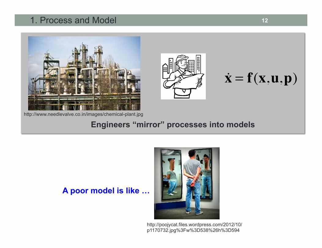
zin (t)
zout (t)
Z(t)
rgen (t)rcon (t)
zin :Rate of INPUTzout :Rate of OUTPUTrgen :Rate of GENERATIONrcon :Rate of CONSUMPTIONZ : Physical quantity of interest
zint
t+Δt
∫ (t)dt + rgen (t)dtt
t+Δt
∫ − zout (t)dtt
t+Δt
∫ − rcon (t)dtt
t+Δt
∫ = Z(t + Δt)− Z(t)
Integral Balance – Mathematical Representation 26

From Integral Balance to Differential Balance 2. Formulating Fundamental Models
Input Output Input
zin (t)+ rgen (t)− zout (t)− rcon (t) =dZ(t)dt
or dZdt
= zin + rgen − zout − rcon⎛⎝⎜
⎞⎠⎟
Integral balance:
Differential balance:
zin (t)
zout (t)
Z(t)
rgen (t)rcon (t)
zin :Rate of INPUTzout :Rate of OUTPUTrgen :Rate of GENERATIONrcon :Rate of CONSUMPTIONZ : Physical quantity of interest
zint
t+Δt
∫ (t)dt + rgen (t)dtt
t+Δt
∫ − zout (t)dtt
t+Δt
∫ − rcon (t)dtt
t+Δt
∫ = Z(t + Δt)− Z(t)
Rate ofINPUT
⎛⎝⎜
⎞⎠⎟+
Rate of GENERATION
⎛⎝⎜
⎞⎠⎟−
Rate of OUTPUT
⎛⎝⎜
⎞⎠⎟−
Rate of CONSUMPTION
⎛⎝⎜
⎞⎠⎟=
Rate of ACCUMULATION
⎛⎝⎜
⎞⎠⎟
27

2. Formulating Fundamental Models
Input Output Input
Differential balance at steady-state –> Rate of ACCUMULATION becomes 0
Rate ofINPUT!
"#
$
%&+
Rate ofGENERATION!
"#
$
%&−
Rate ofOUTPUT!
"#
$
%&−
Rate ofCONSUMPTION!
"#
$
%&= 0
Conservation Laws – Differential Balance at Steady State
zin (t)
zout (t)
Z(t)
rgen (t)rcon (t)
zin :Rate of INPUTzout :Rate of OUTPUTrgen :Rate of GENERATIONrcon :Rate of CONSUMPTIONZ : Physical quantity of interest
zin + rgen − zout − rcon = 0 Now we know better why we can do this in CHEE 221!
28

Differential Balance as General Form of Balance Equations 2. Formulating Fundamental Models
Input Output Input
dZdt
= zin + rgen − zout − rcon
zin (t)
zout (t)
Z(t)
rgen (t)rcon (t)
Rate of INPUT: zin= ρFin
Rate of OUTPUT: zout = ρFout
Rate of GENERATION: rgen= 0Rate of CONSUMPTION: rcon = 0Rate of ACCUMULATION: dZdt
= d(ρAh)dt
Rate of ACCUMULATION
⎛⎝⎜
⎞⎠⎟
=Rate ofINPUT
⎛⎝⎜
⎞⎠⎟+
Rate of GENERATION
⎛⎝⎜
⎞⎠⎟−
Rate of OUTPUT
⎛⎝⎜
⎞⎠⎟−
Rate of CONSUMPTION
⎛⎝⎜
⎞⎠⎟
d(ρAh)dt
= ρFin − ρFout
Fin (m3/s)
Fout (m3/s)
h (m)
29

2. Formulating Fundamental Models
Input Output Input
Material Balance – Example 1 F1 (m3 /min)
F3 (m3 /min)C3 (mol/m3)
C1 (mol/m3) • Well-mixed tank. • All streams have a constant density ρ • C1, C2, C3 are concentrations of a key
component A.
F2 (m3 /min)
C2 (mol/m3)
A (m2 )
h (m) Develop mass balance equations for the total mass and component A in the tank.
30
dhdt
= F1 + F2 − F3A
dC3
dt= F1Ah
C1 +F2Ah
C2 −F1 + F2Ah
C3

2. Formulating Fundamental Models
Input Output Input
Material Balance – Example 2 F1 (L/s)
F (L/s)
CA (mol/L)
CA1 (mol/L)
V (L)
• Stirred tank reactor, well-mixed. • A chemical A reacts to produce a
chemical B. Rate of reaction of A is rA=kCA (mol/s/L).
• All fluids have a constant density of ρ.
1. Develop mass balance equations for the total mass and component A in the tank.
2. Let V=1 L, F1=1 L/s, CA1=1 mol/L, k=1 s-1 and they are all constant over time. a) What is the concentration of A in the tank at the steady state? b) If the concentration of A in the tank is 0 mol/L at a time instant, what is the concentration of A in the tank after 0.01 minute? Keep 4 digits after the decimal point.
31
A→ B

2. Formulating Fundamental Models
Input Output Input
Material Balance – Example 3
• Well-mixed tank, liquid volume V • C1, C2, C, mass fractions of a
component A • ρ1, ρ2, ρ, densities • F1, F2, F, volumetric flow rates • V is constant
Develop a dynamic model with mass balance equations for the following cases: Case 1: ρ1= ρ2= ρ are constant; Case 2: Density varies linearly with mass fraction of A.
F,C,ρ
F2,C2,ρ2F1,C1,ρ1
V
32
- This is Problem 3 of Tutorial 2 - A follow-up question is Problem 1 of Problem Set 1

2. Formulating Fundamental Models
Material Balance – Physical Quantity of Interest is Mass
Rate of massINPUT!
"#
$
%&−
Rate of massOUTPUT!
"#
$
%&=
Rate of massACCUMULATION!
"#
$
%&
Conceptual form for material balance:
(A) Total mass balance
Rate of componentmass INPUT!
"#
$
%&+
Rate of componentmass GENERATION!
"#
$
%&−
Rate of componentmass OUTPUT!
"#
$
%&
−Rate of componentmass CONSUMPTION!
"#
$
%&=
Rate of componentmass ACCUMULATION!
"#
$
%&
(B.1) Mass balance of a component (nonreactive process)
Rate of componentmass INPUT!
"#
$
%&−
Rate of componentmass OUTPUT!
"#
$
%&=
Rate of componentmass ACCUMULATION!
"#
$
%&
(B.2) Mass balance of a component (reactive process) Mole balance can be used here directly (as the molar mass of the component is constant)
General conceptual form for conservation laws: Rate ofINPUT!
"#
$
%&+
Rate ofGENERATION!
"#
$
%&−
Rate ofOUTPUT!
"#
$
%&−
Rate ofCONSUMPTION!
"#
$
%&=
Rate ofACCUMULATION!
"#
$
%&
33

2. Formulating Fundamental Models
Energy Balance – Quantity of Interest is Energy
Rate of energyINPUT!
"#
$
%&−
Rate of energyOUTPUT!
"#
$
%&=
Rate of energyACCUMULATION!
"#
$
%&
Conceptual form for energy balance:
General conceptual form for conservation laws: Rate ofINPUT!
"#
$
%&+
Rate ofGENERATION!
"#
$
%&−
Rate ofOUTPUT!
"#
$
%&−
Rate ofCONSUMPTION!
"#
$
%&=
Rate ofACCUMULATION!
"#
$
%&
outinsys EEdtdE !! −=
where =dtdEsys
=inE!
=outE!
Rate of change of the energy stored in the system
Rate at which energy enters the system
Rate at which energy leaves the system
(1)
34
* CHEE 221 textbook is a good reference for energy balance.

2. Formulating Fundamental Models
Energy Balance – Quantity of Interest is Energy
35
In order to simplify the subsequent discussion, only systems with one inlet flow and one outlet flow are considered …

2. Formulating Fundamental Models
Energy Balance – An Enthalpy Form With Assumption 1
H sys : Specific enthalpy of the system, unit: energy/massmsys : Total mass of the system, unit: mass
Hin : Specific enthalpy of the input, unit: energy/mass!min : Rate of mass input, unit: mass/timeQin : Rate of heat input, unit: energy/time
Hout : Specific enthalpy of the output, unit: energy/mass!mout : Rate of mass output, unit: mass/timeQout : Rate of heat output, unit: energy/time
Assumption 1: Energy change of a system equals to enthalpy change of the system. (i.e., Kinetic energy, potential energy, and work done to and by the system are not considered.)
dEsys
dt=d msysH sys( )
dt
Ein − Eout = minHin − mout Hout + Qin − Qout
Therefore, the energy balance can be written as follows:
d msysH sys( )dt
= !minHin − !mout Hout + Qin − Qout(2)
36

2. Formulating Fundamental Models
Energy Balance – An Enthalpy Form With Assumptions 1 and 2
Assumption 2: The system is a lumped parameter system. H sys = Hout
With Assumptions 1 and 2, the energy balance becomes
d msysHout( )dt
= minHin − mout Hout + Qin −Qout
dHout
dt=!min
msys
H in − Hout( )+ Qin −Qout
msys
Why?
(3)
37

2. Formulating Fundamental Models
Energy Balance – A Temperature Form With Assumptions 1, 2 and 3
Assumption 3: No phase changes take place in the system, and the input and output materials have the same constant specific heat capacity Cp
Hin − Hout ≈Cp Tin −Tout( )
dHout
dt= Cp
dToutdt
+ Δ !Hr
msys Δ Hr : Rate of enthalpy change due to the reaction: energy/time
With Assumptions 1, 2 and 3, the energy balance becomes
dToutdt
=!min
msys
Tin −Tout( )− Δ !Hr
Cpmsys
+Qin −Qout
Cpmsys(4)
38

2. Formulating Fundamental Models
Energy Balance – Summary
outinsys EEdtdE !! −= (1)
(4)
Assumption 1
Assumption 3
d msysH sys( )dt
= minHin − mout Hout + Qin − Qout(2)
dHout
dt=min
msys
H in − Hout( )+ Qin −Qout
msys
(3)
Assumption 2
dToutdt
=min
msys
Tin −Tout( )− Δ Hr
Cpmsys
+Qin −Qout
Cpmsys
39

2. Formulating Fundamental Models
Energy Balance – Stirred Tank Heater
F1 (L/s)
F (L/s) T (K)
T1 (K)
V (L)
Consider a perfectly mixed stirred-tank heater, with a single feed stream and a single product stream. The tank is perfectly insulated, and the rate of the heat added is Q. The volume of liquid in the tank (V) is constant, and the density of the liquid (ρ) does not change with temperature. Develop a model to find the tank temperature as a function of T1, F1, Q, and time, and state the assumptions.
Q (J/s)
dTdt
= F1V
T1 −T( ) + QCpρV
40
Practice problems
41
• Problem Set 1 - Problem 1 - Problem 2 - Problem 3 (a)(b)(c)

2. Formulating Fundamental Models
Constitutive Relationships – Ideal Gas Law
§ Ideal Gas Law
PV = nRT Note: P is absolute pressure, T is in Kelvin.
dPdt
=RTV
q1 − q( )
42
Gas surge drum
V (L), T (K) constantq1 (mol/min) q (mol/min)
Objective: To develop a model describing how drum pressure P changes with time.
Example:

2. Formulating Fundamental Models
Constitutive Relationships – Chemical Reaction Kinetics (1) § Chemical Reaction Kinetics - How fast the reaction is? (CHEE 321)
Reaction A + B à 2C
Definition of Rate of Reaction:
rA ≡ − dCA
dt, rB ≡ − dCB
dt, rC ≡ dCC
dt (mol/(L ⋅min))
(http://chemistry.tutorvista.com/physical-chemistry/collision-theory.html)
“Valid” collision with sufficient collision energy
(http://www.drroyspencer.com/2010/06/) Random movement of molecules Reaction via collision of molecules
“Invalid” collision without sufficient collision energy
43

2. Formulating Fundamental Models
Constitutive Relationships – Chemical Reaction Kinetics (2) § Chemical Reaction Kinetics - How fast the reaction is? (CHEE 321)
Reaction A + B à 2C
Definition of Rate of Reaction:
If rA = kCAmCB
n , the reacation is mth order in A and nth order in B.
rA ≡ − dCA
dt, rB ≡ − dCB
dt, rC ≡ dCC
dt (mol/(L ⋅min))
Order of Reaction:
k = koe−E /RT ,
where E = the activation energy (constant) R = gas constant ko= Pre-exponential constant
k is constant for isothermal reactors.
Arrhenius Equation:
44

2. Formulating Fundamental Models
Constitutive Relationships – Heat Transfer
§ Three heat transfer modes
45
http://www.spectrose.com/wp-content/uploads/2012/12/modes-of-heat-transfer-conduction-convection-and-radiation.jpg

2. Formulating Fundamental Models
Constitutive Relationships – Heat Transfer
§ Rate of Heat Transfer – for conduction and convection
Q =UAΔT
where Q = rate of heat transferred from the hot object to the cold object U = overall heat transfer coefficient A = area for heat transfer ΔT = difference between the temperatures of the hot and cold objects
46
F1,T1
F,T
Fc ,Tc,in cooling water
Cooling jacket Cooling coil
F1,T1
F,Tcooling waterTc,in ,Fc

2. Formulating Fundamental Models
Thoughts on modeling …
1. What is the system?
2. What are the mass/material balance relationships? What are the energy balance relationships? What are the constitutive relationships? 3. What are the assumptions?
Practice and practice!
Questions to be answered during the development of a mathematical model:
47

2. Formulating Fundamental Models
Nonisothermal Continuous Stirred Tank Reactor (CSTR)
• Well mixed reactor, insulated. • Constant volume V. • Constant specific heat capacity Cp (kJ/(kg*K))
and density ρ (kg/L). • Exothermic reaction AàB, first-order in A,
heat of reaction ΔH (kJ/mol). • The cooling flowrate Fc is constant, and the
rate of heat transfer Q (kJ/min) between the liquid in the tank and the cooling coil satisfies:
Q = UA(T-Tin)
Objective: To develop a model describing the dynamic behavior of CA and T. State assumptions made for the model.
dCA
dt= FV
CA1 −CA( )− koe−E /(RT )CA
dTdt
= FVT1 −T( )− ΔH
ρCp
koe−E /(RT )CA −
UAρVCp
T −Tin( )
F (L/min)T (K)
V (L)
Fc (L/min)
Tin (K) Tout (K)
CA1 (mol/L)
F1 (L/min) T1 (K)
CA (mol/L)
A→ B
48
2. Formulating Fundamental Models
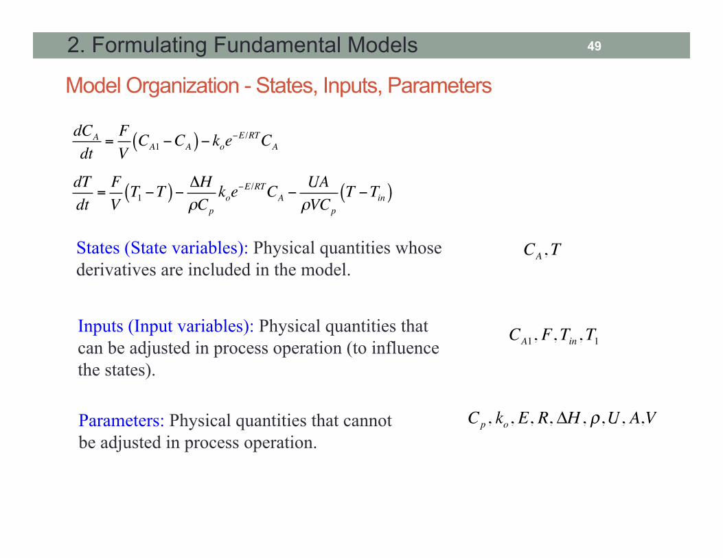
Model Organization - States, Inputs, Parameters
dCA
dt=FV
CA1 −CA( )− koe−E /RTCA
dTdt
=FV
T1 −T( )− ΔHρCp
koe−E /RTCA −
UAρVCp
T −Tin( )
Cp , ko, E, R, ΔH , ρ,U, A,VParameters: Physical quantities that cannot be adjusted in process operation.
49
States (State variables): Physical quantities whose derivatives are included in the model.
CA ,T
Inputs (Input variables): Physical quantities that can be adjusted in process operation (to influence the states).
CA1, F,Tin ,T1

2. Formulating Fundamental Models
Model Organization - States, Inputs, Parameters
dh1dt
=F0A1−βA1h1
dh2dt
=βA2h1 −
βA2h2
F0
h1
h2A1
A2
F1h1=F2h2= β
F1
F2
States: h1, h2 Inputs: F0 Parameters: β, A1, A2
States: T Inputs: F1, T1, Q Parameters: V, ρ, Cp
F1 (L/s)
F (L/s)T (K)
T1 (K)
V (L)
Q (J/s)
dTdt
= F1V
T1 −T( ) + QCpρV
V is constant.
50

2. Formulating Fundamental Models
Model Organization - Dimensionless Model
dCA
dt= F1V(CA1 −CA )− kCA
Let x = CA
CA10
, x f =CA1
CA10
, τ = FVt (All have no units!)
dxdτ
= x f − 1+VkF
"
#$
%
&'x
A→ B
F1 (L/min), CA1 (mol/L), T1 (K)
V (L)
Isothermal reactor
F (L/min), CA (mol/L), T (K)
51
F1 = F = constant
- States and Inputs have no units! - Parameters may have units.

2. Formulating Fundamental Models
Model Organization - General Form of Dynamic Models
x1 = f1(x1,…, xn,u1,…,um, p1,…, pr )x2 = f2 (x1,…, xn,u1,…,um, p1,…, pr )xn = fn (x1,…, xn,u1,…,um, p1,…, pr )
x = f(x,u,p) (more convenient on computers)
x = f (x,u, p)(more convenient for hand-writing)
52
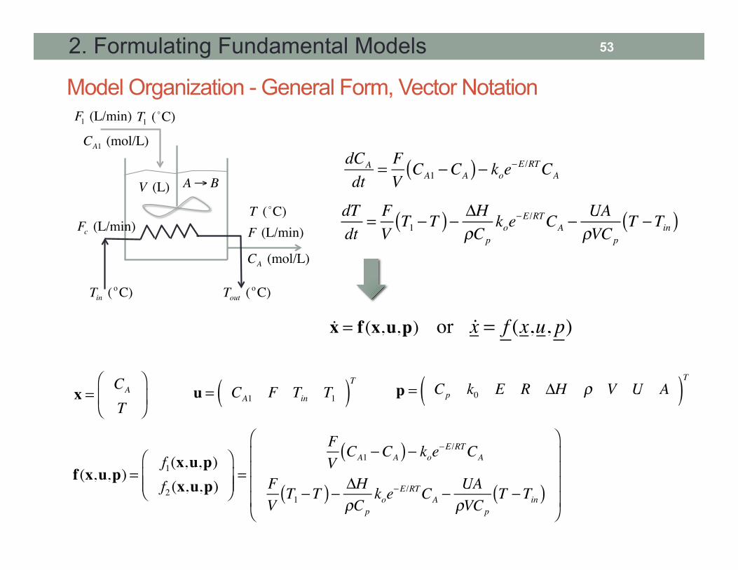
2. Formulating Fundamental Models
Model Organization - General Form, Vector Notation
dCA
dt= FV
CA1 −CA( )− koe−E /RTCA
dTdt
= FVT1 −T( )− ΔH
ρCp
koe−E /RTCA −
UAρVCp
T −Tin( )
x = f(x,u,p)
x = CA
T
⎛
⎝⎜
⎞
⎠⎟ u = CA1 F Tin T1( )T p = Cp k0 E R ΔH ρ V U A( )T
f(x,u,p) =f1(x,u,p)f2 (x,u,p)
⎛
⎝⎜⎜
⎞
⎠⎟⎟=
FV
CA1 −CA( )− koe−E /RTCA
FVT1 −T( )− ΔH
ρCp
koe−E /RTCA −
UAρVCp
T −Tin( )
⎛
⎝
⎜⎜⎜⎜
⎞
⎠
⎟⎟⎟⎟
F (L/min)T ( C)
V (L)
Fc (L/min)
Tin ( o C) Tout (o C)
CA1 (mol/L)
F1 (L/min) T1 ( C)
CA (mol/L)
A→ B
or x = f (x,u, p)
53

2. Formulating Fundamental Models
54
f(x) =f1(CA ,T )f2 (CA ,T )
⎛
⎝⎜
⎞
⎠⎟ =
FV
CAf −CA( )− k0 exp −ERTr
⎛⎝⎜
⎞⎠⎟CA
FVTf −T( )− ΔH
ρCp
k0 exp−ERT
⎛⎝⎜
⎞⎠⎟CA −
UAρVCp
T −Tj( )
⎛
⎝
⎜⎜⎜⎜⎜
⎞
⎠
⎟⎟⎟⎟⎟

2. Formulating Fundamental Models
55
f(x) =f1(CA ,T )f2 (CA ,T )
⎛
⎝⎜
⎞
⎠⎟ =
FV
CAf −CA( )− k0 exp −ERTr
⎛⎝⎜
⎞⎠⎟CA
FVTf −T( )− ΔH
ρCp
k0 exp−ERT
⎛⎝⎜
⎞⎠⎟CA −
UAρVCp
T −Tj( )
⎛
⎝
⎜⎜⎜⎜⎜
⎞
⎠
⎟⎟⎟⎟⎟

2. Formulating Fundamental Models
Model Organization - General Form, Vector Notation
dh1dt
=F0A1−βA1h1
dh2dt
=βA2h1 −
βA2h2
dh1dtdh2dt
!
"
####
$
%
&&&&
=
−βA1
0
βA2
−βA2
!
"
#####
$
%
&&&&&
h1h2
!
"
##
$
%
&&+
1A10
!
"
###
$
%
&&&F0
F0
h1
h2A1
A2F1h1=F2h2= β
F1
F2
x = Ax +Bu or x = Ax + Bu
56

Practice problems
57
• Problem Set 1 - Problem 1 - Problem 2 - Problem 3 - Problem 4 - Problem 5