Charting A Mathematical Equation Using ExcelAnd Defined Names

Introduction

When doing mathematics, wouldn't it be nice if we could type anequation into a cell in Excel and immediately see the resultinggraph?

Suppose we have an equation like:

y=x2-2.x+6

Normally, we would create a column with x values and in theadjacent column "translate" this formula into a cell formula:

=A2^2-2*A2+6

and copy this formula down to match the number of x values incolumn A:

Subsequently, we would base a chart on this set of data:

 

 This method lacks flexibility. It would be much more convenient, if we could:

• Enter the (any!) formula into a single cell

• Enter the lower and upper limit of the x-range into two othercells

• Enter the number of values to use for the chart in yetanother cell:

 

 Yet another constraint we're going to place on this task:

Apart from the cells shown in the figure above, no cells are to beused, just defined names with formulas.

Create the Chart

Because we cannot start creating a chart without data, simplyadd some data to a couple of cells:

 

and click the chart wizard button. Make sure to select the "XY(scatter)" chart type and hit Finish.

Now define two names local to the worksheet the chart is on:

Name Refers To

Sheet1

!x

$A$12:$A$

15

Sheet1

!y

$B$12:$B$

15

Now we need to use these two defined names in the chart'sSERIES formula (click the line in the chart and then click theformula bar), currently looking like this:

(Note this shows the SERIES formula as I see it, with thesemicolon as list separator.)

Edit this formula so it looks like this:

=SERIES(Sheet1!$B$8,Sheet1!x,Sheet1!y,1)

Cell B8 will contain the chart's title, so we'll put this little formulain B8:

="Charting: " & Sheet1!$B$1

Getting x values

 The next task is to get a list if x values we can use for the x-axesof the chart. A little known fact, is that when a defined name isused to name a formula this formula will be an array formula bydefault. We're going to put that to use.

 

First we need a set of incrementing numbers. We'll use the ROWworksheet function for that.

When we define this name local to worksheet Sheet1:

Name: Sheet1!x

RefersTo: =ROW(1:20)

and we enter an array formula into cells A1:A20 (select A1:A20 inSheet1 and type =x, then hit control-shift-enter) we get thisresult:

But we want the number of x-values to be dependent on anumber entered into a cell. We'll use the OFFSET worksheetfunction for this purpose:

=ROW(OFFSET(Sheet1!$A$1,0,0,20,1))

If we replace the previous formula in "Sheet1!x" with the oneabove, the result will remain the same as shown above.All it takes now is replace the fixed 20 with a cell reference:

=ROW(OFFSET(Sheet1!$A$1,0,0,Sheet1!$B$5,1))

 

Now we have the numbers 1 to 20 (or up to whatever number weenter into cell B5 on sheet1).

But we need more flexibility, we want to be able to set aminimum and a maximum value for x and use the 1-20 range tospace out these limits.

Let's define these named ranges:

Name Refers To

xStart=Sheet1!

$B$3

xEnd=Sheet1!

$B$4

xNumberOfPoi

nts

=Sheet1!

$B$5

xRange=xEnd-

xStart

 To get a series of "xNumberOfPoints" from xStart to xEnd, the

following formula applies:

xPoint=xStart+xRange/(xNumberOfPoints-1)*Counter(1 toxNumberOfPoints-1)

So applying the approach depicted above:

=xStart+xRange/(xNumberOfPoints-1)*(ROW(OFFSET(Sheet1!$A$1,0,0,xNumberOfPoints,1))-1)

We'll name this new formula (surprisingly): Sheet1!x

Getting y values

Now that we have gotten a dynamic set of x values it is time toderive results. Again we'll define a named range:

 

Name Refers To

Formul

a

=Sheet1!

$B$1

What we need is a mechanism to evaluate the formula in cell B1using the x values we have available. For this we'll use the factthat Excel accepts ancient xl4 macro functions inside definednames. The function needed is the EVALUATE function, which weuse in the name y, local to worksheet Sheet1:

Name Refers To

Sheet1

!y

=EVALUATE(Formu

la)

Strange enough, this version of y only seems to work for functionsthat do not use built-in Excel functions like SIN or COS, usingthose in the function will cause Excel to compute all constantvalues, regardless of the x's!

Stephen Bullen has created an almost identical version of thisworkbook a long time ago, using Excel 5. Look for a downloadcalledChtFrmla.zip. He used a trick to make these functions workby adding "0*x" to the set of y values:

Name Refers To

Sheet1

!y

=EVALUATE(Formula&"+0

*x")

Suddenly, including Excel functions has become possible!

Using Controls On Worksheets

Where to find the controls

 

Excel 2007 and up

In Excel 2007 and later versions, the form controls and controltoolbox controls are slightly hidden. First of all, you need to showthe "Developer" tab of the ribbon. Here is how that's done:

• Click the Office button and select "Excel options..." (for Excel2010 and up: Click File, Options and then locate this optionon the "Customize ribbon" tab).

• Click the "Popular" tab and check the box next to "ShowDeveloper tab in the ribbon":

Fig 1: Showing the Developer tab on the ribbon (Excel 2010 and up).

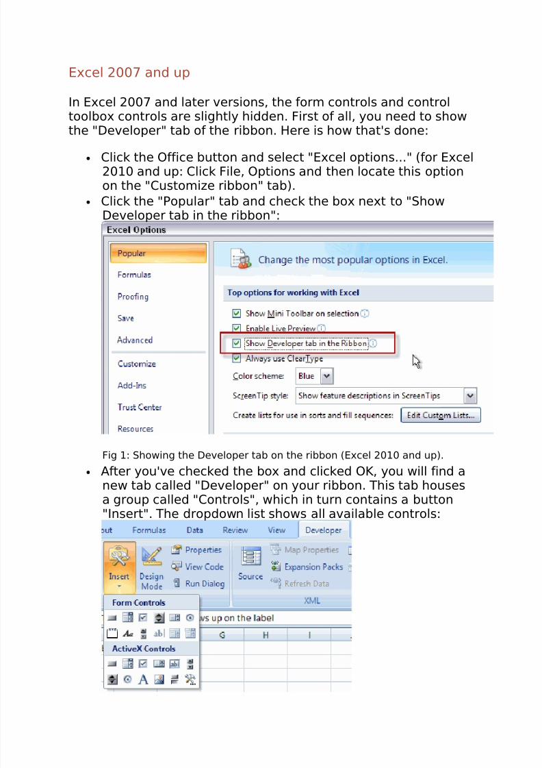
• After you've checked the box and clicked OK, you will find anew tab called "Developer" on your ribbon. This tab housesa group called "Controls", which in turn contains a button"Insert". The dropdown list shows all available controls:

 

Fig. 2: The controls on the Developer tab.

Excel 97-2003

In older Excel versions the controls are housed on two toolbars;the "Forms" toolbar and the "Control toolbox" toolbar. You canshow both toolbars using the menu "View", "Toolbars":

 

Fig. 3: Access to the controls toolbars in Excel 97-2003.

After turning on these two toolbars they are shown:

Fig. 4: The control toolbars in Excel 97-2003.

Two groups of controls; the differences

 

By now it is apparent that there are two distinct series of controls: Those from the forms group and those from the Control toolbox(named ActiveX controls in Excel 2007 and up).

Pro's and con's

 The table below lists some advantages and disadvantages of bothcontrol sets:

Control type Form controls ActiveX controls

Advantages

• Simple to use

• Can be used on chart sheets

• Assigning control to a macro is simple

• Little known problems

• Lots of opti

• Lots of eve

• Lots of for

• Lists returnthan the in

Disadvantag

es• Lists return the index number rather

than the selected value

• Cumbersomultiple co

• Sometimescorruptions

Which should you use

By now you'll be wondering which set you should use. Generallyspeaking, I recommend using the controls from the forms toolbar.If you have specific needs regarding formatting which cannot beachieved using the forms controls (or if you want to programevents in VBA), then you'll have to switch to the ActiveX controls(control toolbox controls).

Inserting controls

Inserting a control on your sheet is very simple: Just click thecontrol you need (See fig. 2 and 4 on the previous page) and draga rectangle on the sheet at the position where you want thecontrol to appear. You can also just click on the sheet and haveExcel decide what dimensions to use for the control.

If you hold down the alt key when you click on the worksheet,then the control will be aligned to the cell grid. You can also holdthe alt key when you are dragging the control or resizing the

 

control to have it snap to the grid. This is a quick way to ensureyour controls are nicely aligned and of equal size.

Double click a control on the toolbar or on the Insert controlsdropdown if you want to draw multiple copies of that control.Click that control again (or any other control) to get out of thatmode.

Overview of the available controls

 The table below shows which controls there are and describeseach one shortly.

Pic

.Control name Control use and remarks

Label Add a label next to other controls.

FrameUse this control to group other controls. OptionB

work together.

Button(CommandButt

on)Start a macro

CheckBox Set an option, Select multiple options from a list o

OptionButton Select one option from a (short) list.

ListBox  Select an option from a list. Multiple options are v

ComboBox Select an option from a list, only the selected opti

ScrollBar Quickly change numeric values.

Spinner Change values step-by-step easily.

 

TextBox Enter a text.

 T oggleButton  Toggle status. This control is not recommended, I

checkbox or a set of two OptionButtons.

Detailed description of the controls (1)

Label

 The label control is the simplest control available, all it can beused for is to display descriptive text. Use this control if you wantto add some explanatory text to another control.

 TIP: You can make sure the label text is derived from aworksheet cell. To do so, select the label and then click in theformula bar and enter a reference to the cell. See fig. 5.

Fig 5: The text on a label drawn from a worksheet cell

Frame

 You can use a frame to visually group controls with a sharedpurpose. Apart from that, the frame control has a specific functionfor option button controls (see the appropriate section aboutthem). You must start with drawing the frame control beforeadding the controls you want placed "inside" the frame. To makethis a painless process, start out by drawing a relatively largeframe (you can make the frame smaller later on). After that, drawthe controls inside the frame:

 

Fig 6: Frames with OptionButtons within.

Button (CommandButton)

Buttons or CommandButtons are used to start VBA code(macro's). If you draw a Button from the Forms toolbar on a sheet,Excel will prompt you for a macro to run when the button isclicked (fig 7). If you have not written a macro yet, then you cantype the macro's name and click the "New" button to have the(empty) subroutine created for you:

Fig 7: Excel asks you what macro to run when the button is clicked.

If you used the CommandButton from the Control toolbox, youneed to double-click the button (in design mode) to access it's

 

VBA click event. Code for control toolbox (ActiveX) controls istypically written in the code module behind the sheet they areplaced on.

 TIP: If you want to change the properties of a control from thecontrol toolbox (an ActiveX control), then you must put yoursheet into "Design mode". In Excel 2003 you can click the firstbutton on the control toolbox toolbar. In Excel 2007 and up youcan find this button on the "Developer" tab, within the "Controls"group. When you want to start using the controls, click the samebutton to get out of design mode.

Detailed description of the controls (2)

CheckBox

 Typically, a checkbox control is used to enable the user to turnsomething on or off, or to answer a yes/no question. Thecheckbox always stands on its own, allowing multiple options tobe selected (checked) at the same time.

OptionButton

 The option button is very similar to the check box, but only allowsmutually exclusive choices to be made; in a set of option buttons,only one option can be "checked". If you take no specific actionthen all option buttons on one sheet will be treated as one singlegroup. It is possible to have multiple groups on a sheet. Themethod to achieve this differs between the two sets of optionbuttons.

 The method to tie an option button to a cell differs between thetwo types too.

Forms option button

 To group option buttons from the forms toolbar, first draw frameson your sheet. Then draw the option buttons INSIDE the frame:

 

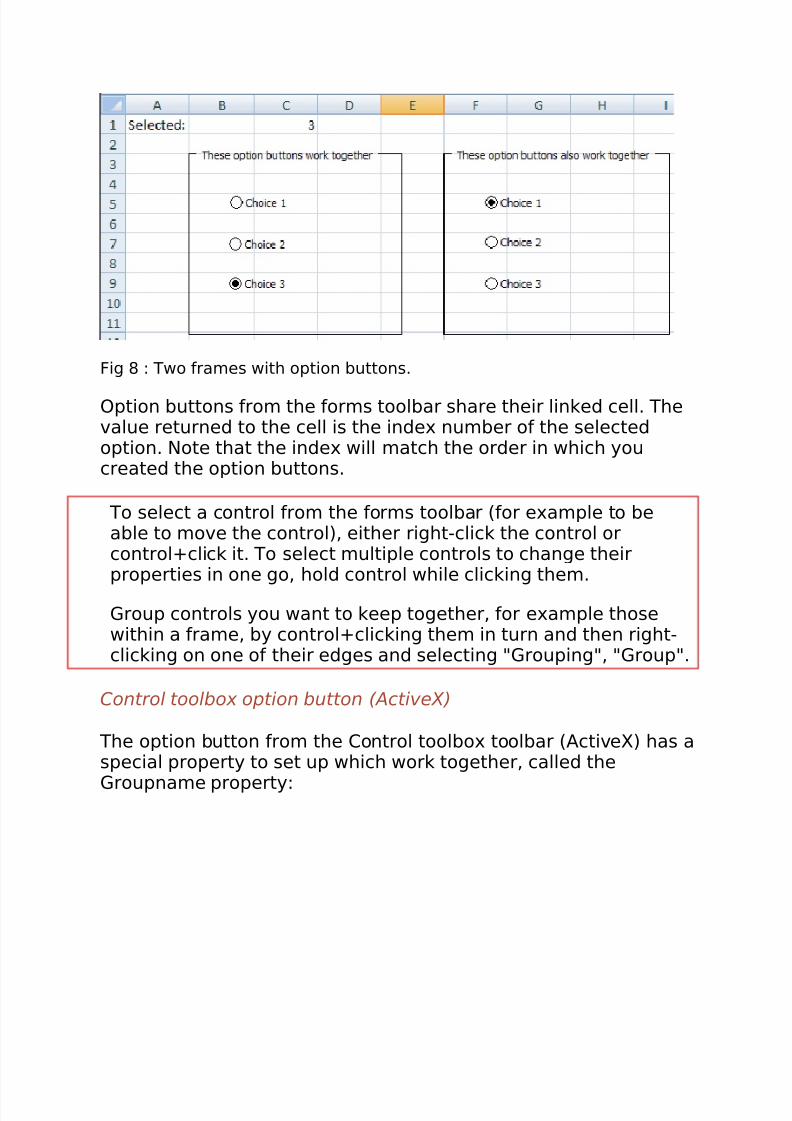
Fig 8 : Two frames with option buttons.

Option buttons from the forms toolbar share their linked cell. Thevalue returned to the cell is the index number of the selectedoption. Note that the index will match the order in which youcreated the option buttons.

 To select a control from the forms toolbar (for example to beable to move the control), either right-click the control orcontrol+click it. To select multiple controls to change theirproperties in one go, hold control while clicking them.

Group controls you want to keep together, for example thosewithin a frame, by control+clicking them in turn and then right-clicking on one of their edges and selecting "Grouping", "Group".

Control toolbox option button (ActiveX)

 The option button from the Control toolbox toolbar (ActiveX) has aspecial property to set up which work together, called theGroupname property:

 

Fig 9: Groupname property of the ActiveX OptionButton control.

If you do not change this property, all option buttons on a sheetwork together as a single group.

ActiveX option buttons all have their own linked cell, which willreceive the checked state of their parents as a True/False value.

 TIP: You can get at the properties window of the controls byright-clicking a control and selecting "Properties". You can alsoclick the appropriate button on the Control Toolbox toolbar. InExcel 2007 and up, you'll find that button on the Developer tab,within the Controls group.

Detailed description of the controls (3)

ListBox

If you want to enable your user to select an option from a list youcan use a list box. Of course you could also use a set of optionbuttons for this goal, but making a set of option buttons dynamic(for example if you want to be able to expand the number of choices) is cumbersome. If you have a limited set of availablechoices (rule of thumb: no more than 5), use option buttons. If there are more, use a list box or a combo box control.

 

 You can either have the control pick up the list from a range of cells, or add the choices to the list box control using VBA. This isdone by entering the corresponding information into theListFillRange or Input range property. If your list of choices resideson a different worksheet from the one your list box is placed on,you must define a range name for the list. Do so by selecting thelist and hitting control+F3. In Excel 2007 and up you then need toclick the "Add" button. Enter a name for the list and click OK untilyou're back in Excel. After that, you can enter this new rangename in the appropriate property of the control.

 The second most important property is the LinkedCell (cell link),this cell will receive the result of selecting an item in the list box:

Fig 10, Two important propeties of the ActiveX list box control.

 

Fig 11: Two important properties of the forms list box.

Note that the list box from the forms toolbar will show the indexof the chosen item in the cell, whereas the control from thecontrol toolbox returns the actual value to the cell. For the list boxfrom the forms toolbar, use a formula like this one to get theactual value:

=INDEX(ListForComboAndList,C1)

 You can set the list box to "Multi" or "Extended" to enablemultiple selections. In that case, the linked cell will show either azero for the list box from the forms toolbar or #N/A for the controltoolbox list box control. You will have to use VBA to read whatitems have been selected and act accordingly.

ComboBox

A combobox is very useful when there are many values to choosefrom and when you only want to show the chosen item. With thecombobox from the Control toolbox you can dynamically additems to the list -using VBA- when the user types a new item inthe box instead of selecting an existing item. The combo box form

 

the forms toolbar does not have this possibility: the user is limitedto the choices available in the list.

 The two important properties LinkedCell and ListFillRange operatein the exact same way as for the list box control.

Detailed description of the controls (4)

ScrollBar

 The most important reason to use a scrollbar is to be able tochange a value very quickly. The user can drag the scroll button,click next to the scroll button to change "page" or click the arrowsto increase or decrease the value stepwise.

Fig 12: Scrollbar with linked cell.

A vertically placed scroll bar works opposite compared to aspinner control. Clicking the up arrow on a spinner increases thevalue; clicking the up arrow on a scroll bar decreases the value.In my opinion, the former is more intuitive. If I need this verticalsetup, I prefer to use a spinner over a scroll bar.

A scroll bar enables you to change the value in two ways. The"Incremental change" is performed by clicking the arrow buttons,the "Page change" is performed by clicking next to the scrollbutton. See fig. 13:

 

Fig 13, Two levels of step sizes.

 These properties have a different name for the scroll bar of theControl Toolbox toolbar (ActiveX) "SmallChange" and"LargeChange" respectively, see figure 14:

 

Fig 14, Setting properties of the ActiveX controls scroll bar.

Scroll bars can only work with integers. The range you can usediffers between the two families. The forms control ranges from 0to 30,000. The ActiveX control can go as high as 666,666.

If you need steps less than 1, then use a calculation. Forexample if you need a step size of 0.5, divide the linked cell'svalue by 2.

Spinner

If you want to be able to quickly change a cell value stepwise, thespinner is the place to be.

 

Fig 15: Spinner controls.

Setting up spinner controls works identical to the scroll barcontrol, using the same properties. Of course the spinner does nothave a Page change (LargeChange) property.

 TextBox

 There is only one text box control, member of the ActiveX familyof controls, on the Control Toolbox toolbar in Excel 2003 andbefore. I find this control to have little use, because you cansimply use a cell and enter text into the cell directly.

 ToggleButton

 The last control I discuss here is the toggle button. This is anotherexample of a control that is only available through the ActiveXfamily of controls. In my opinion, this control is ambiguous. Itcould be used to either indicate an action, or a state. You coulduse a control like this to change the page setup of a sheet fromportrait to landscape and vice versa. Disadvantage of this controlis that the state and action paradigm are conflicting, especially if the two states have a different name (like in the example).

Suppose you want to enable toggling between portrait enlandscape. You might be tempted to use a toggle button, whichhas some VBA attached to it to set the option and which updatesthe caption of the control. What does the caption indicate, thecurrent status, or the status AFTER clicking the toggle button?

Fig 16: Ambiguity when using a toggle button: which one indicates we'rein Portrait mode?

Due to this ambiguity a toggle button is only useful to indicate anon or off state for a property which has the same name in bothstates. For this goal, a checkbox is to be preferred. If there aretwo mutually exclusive choices, consider using two optionbuttons.

 

Interaction between controls and worksheet cells

Each control can be tied to a cell and thus (by using that cell inyour formulas) affect your spreadsheet model directly and driveinteractivity between your model and the user. For the formscontrols, you access these options by right-clicking the control inquestion and selecting "Format control". Each control offers itsown set of options, which are located on the "Control" tab.(see figures 11 en 13). Similarly, you can change the properties of the Control toolbox (ActiveX) controls using their propertieswindow.

Conclusion

Excel is a very flexible instrument to perform analyses and what-if scenario’s. You use formulas in cells with one or more input cellsto calculate the various situations. To ease working with differentvalues and/or choices, you can put the controls from either theControl toolbox or the Forms toolbar to good use. Proper use of these controls make your models easier to use.

 The controls also enable you to ease data entry and at the sametime improve data quality by minimizing the risk of wrong entries.For "day-to-day" use, I recommend the Forms controls. If thereare specific options you need which are not offered by the formcontrols then you can also implement the Control toolbox(ActiveX) controls.

Introduction

In Working with Tables in Excel 2013, 2010 and 2007 I promisedto add a page about working with those tables in VBA too. Well,here you go.

It's a ListObject!

On the VBA side there seems to be nothing new about Tables. They are addressed as ListObjects, a collection that wasintroduced with Excel 2003. But there are significant changes tothis part of the object model and I am only going to touch on thebasic parts here.

 

Creating a table

Converting a range to a table starts with the same code as inExcel 2003:

Sub CreateTable()ActiveSheet.ListObjects.Add(xlSrcRange, Range("$B$1:$D$16"), , xlYes).Name

= _"Table1"'No go in 2003

ActiveSheet.ListObjects("Table1").TableStyle = "TableStyleLight2"End Sub

But the new stuff is right there already: TableStyles. A collectionof objects which are a member of the Workbook object. This givesrise to some oddities. You can change the formatting of atableStyle, e.g. like this:

Sub ChangeTableStyles()'No Go in Excel 2003ActiveWorkbook.TableStyles(2).TableStyleElements(xlWholeTable) _

.Borders(xlEdgeBottom).LineStyle = xlDashEnd Sub

 This changes the linestyle of the bottom of your table. But holdyour horses! If you have any other workbook open, all tables withthe same tablestyle appear in your changed style! But if you saveyour file, close Excel and open Excel again with the file, thechanges are gone. This is because you've just changed a built-intablestyle. If you ask me, I find it strange that the Workbook is atablestyles' parent, whereas built-in table styles behave as if being bound to the Application object.

If you want full control over your table style, you'd betterduplicate a built-in style and modify and apply that style to yourtable.

Listing the tables

Let's start with finding all tables on the active worksheet:

Sub FindAllTablesOnSheet()Dim oSh As WorksheetDim oLo As ListObjectSet oSh = ActiveSheetFor Each oLo In oSh.ListObjects

Application.Goto oLo.RangeMsgBox "Table found: " & oLo.Name & ", " & oLo.Range.Address

NextEnd Sub

 

 This snippet of code works exactly the same in Excel 2003, sonothing new there (well, that is, in 2003 those tables ARE calledLists).

Selecting parts of tables

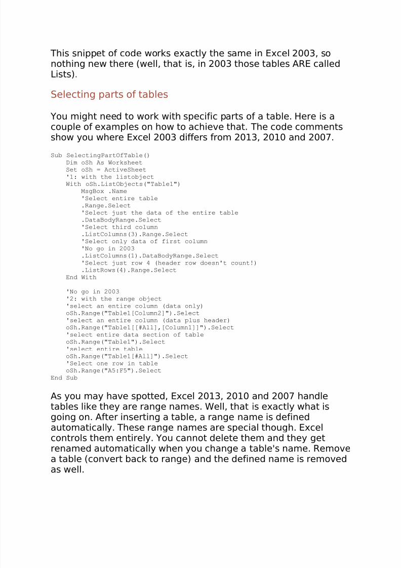
 You might need to work with specific parts of a table. Here is acouple of examples on how to achieve that. The code commentsshow you where Excel 2003 differs from 2013, 2010 and 2007.

Sub SelectingPartOfTable()Dim oSh As WorksheetSet oSh = ActiveSheet'1: with the listobjectWith oSh.ListObjects("Table1")

MsgBox .Name'Select entire table.Range.Select'Select just the data of the entire table.DataBodyRange.Select'Select third column.ListColumns(3).Range.Select'Select only data of first column'No go in 2003.ListColumns(1).DataBodyRange.Select'Select just row 4 (header row doesn't count!).ListRows(4).Range.Select

End With 

'No go in 2003'2: with the range object'select an entire column (data only)oSh.Range("Table1[Column2]").Select'select an entire column (data plus header)oSh.Range("Table1[[#All],[Column1]]").Select'select entire data section of tableoSh.Range("Table1").Select'select entire tableoSh.Range("Table1[#All]").Select'Select one row in tableoSh.Range("A5:F5").Select

End Sub

As you may have spotted, Excel 2013, 2010 and 2007 handletables like they are range names. Well, that is exactly what isgoing on. After inserting a table, a range name is definedautomatically. These range names are special though. Excelcontrols them entirely. You cannot delete them and they getrenamed automatically when you change a table's name. Removea table (convert back to range) and the defined name is removedas well.

 

Inserting rows and columns

Another part in which lists already had most of the functionality. Just a few new things have been added, like the "AlwaysInsert"argument to the ListRows.Add method:

Sub TableInsertingExamples()'insert at specific position

Selection.ListObject.ListColumns.Add Position:=4'insert right

Selection.ListObject.ListColumns.Add'insert above

Selection.ListObject.ListRows.Add (11)'NoGo in 2003'insert below

Selection.ListObject.ListRows.Add AlwaysInsert:=TrueEnd Sub

If you need to do something with a newly inserted row, you canset an object variable to the new row:

Dim oNewRow As ListRowSet oNewRow = Selection.ListObject.ListRows.Add(AlwaysInsert:=True)

If you then want to write something in the first cell of the new rowyou can use:

oNewRow .Range.Cells(1,1).Value="Value For New cell"

Adding a comment to a table

 This is something Excel 2003 cannot do and is related to the factthat a table is a range name. Adding a comment to a tablethrough the UI is a challenge, because you have to go to theName Manager to do that. In VBA the syntax is:

Sub AddComment2Table()Dim oSh As WorksheetSet oSh = ActiveSheet'NoGo in 2003'add a comment to the table (shows as a comment to'the rangename that a table is associated with automatically)'Note that such a range name cannot be deleted!!'The range name is removed as soon as the table is converted to a rangeoSh.ListObjects("Table1").Comment = "This is a table's comment"

End Sub

Convert a table back to a normal range

 That is simple and uses the identical syntax as 2003:

Sub RemoveTableStyle()Dim oSh As Worksheet

 

Set oSh = ActiveSheet'remove table or list styleoSh.ListObjects("Table1").Unlist

End Sub

Special stuff: Sorting and filtering

With Excel 2013, 2010 and 2007 we get a whole new set of filtering and sorting options. I'm only showing a tiny bit here, aSort on cell color (orangish) and a filter on the font color. Thecode below doesn't work in Excel 2003. A List in 2003 only hasthe default sort and autofilter possibilities we have known sinceExcel 5 and which had hardly been expanded at all in the past 12years or so.

Sub SortingAndFiltering()'NoGo in 2003

With ActiveWorkbook.Worksheets("Sheet1").ListObjects("Table1")

.Sort.SortFields.Clear

.Sort.SortFields.Add( _Range("Table1[[#All],[Column2]]"), xlSortOnCellColor,

xlAscending, , _xlSortNormal).SortOnValue.Color = RGB(255, 235, 156)

With .Sort.Header = xlYes.MatchCase = False.Orientation = xlTopToBottom.SortMethod = xlPinYin.Apply

End WithEnd With'Only old autofilter stuff works in 2003ActiveSheet.ListObjects("Table1").Range.AutoFilter Field:=2, _

Criteria1:=RGB(156, 0, 6), Operator:=xlFilterFontColorEnd Sub

Accessing the formatting of a cell inside a table

 You may wonder why this subject is there, why not simply ask forthe cell.Interior.ThemeColor if you need the ThemeColor of a cellin a table? Well, because the cell formatting is completelyprescribed by the settings of your table and the table style thathas been selected. So in order to get at a formatting element of acell in your table you need to:

• Find out where in your table the cell is located (on headerrow, on first column, in the bulk of the table

• Determine the table settings: does it have row stripingturned on, does it have a specially formatted first column, ...

 

• Based on these pieces of information, one can extract theappropriate TableStyleElement from the table style andread its properties.

 The function shown here returns the TableStyleElement belongingto a cell oCell inside a table object called oLo:

Function GetStyleElementFromTableCell(oCell As Range,

oLo As ListObject) As TableStyleElement

'-------------------------------------------------------------------------

' Procedure : GetStyleElementFromTableCell

' Company : JKP Application Development Services (c)

' Author : Jan Karel Pieterse

' Created : 2-6-2009

' Purpose : Function to return the proper style element from a cell inside a

table

'-------------------------------------------------------------------------

  Dim lRow As Long

  Dim lCol As Long

  'Determine on what row we are inside the table

lRow = oCell.Row - oLo.DataBodyRange.Cells(1, 1).Row

lCol = oCell.Column - oLo.DataBodyRange.Cells(1, 1).Column

  With oLo

  If lRow < 0 And .ShowHeaders Then

  'on first row and has header

  Set GetStyleElementFromTableCell =

oLo.TableStyle.TableStyleElements(xlHeaderRow)

  ElseIf .ShowTableStyleFirstColumn And lCol = 0 Then

  'On first column and has first column style

  Set GetStyleElementFromTableCell =

oLo.TableStyle.TableStyleElements(xlFirstColumn)

  ElseIf .ShowTableStyleLastColumn And lCol = oLo.Range.Columns.Count -

1 Then

  'On last column and has last col style

  Set GetStyleElementFromTableCell =

oLo.TableStyle.TableStyleElements(xlLastColumn)

  ElseIf lRow = .DataBodyRange.Rows.Count And .ShowTotals Then

  'On last row and has total row

  Set GetStyleElementFromTableCell =

oLo.TableStyle.TableStyleElements(xlTotalRow)

  Else

  If .ShowTableStyleColumnStripes

And Not .ShowTableStyleRowStripes Then

  'in table, has column stripes

  If lCol Mod 2 = 0 Then

  Set GetStyleElementFromTableCell =

oLo.TableStyle.TableStyleElements(xlColumnStripe1)

  Else

  Set GetStyleElementFromTableCell =

oLo.TableStyle.TableStyleElements(xlWholeTable)

  End If

  ElseIf .ShowTableStyleRowStripes

And Not .ShowTableStyleColumnStripes Then

  'in table, has column stripes

 

  If lRow Mod 2 = 0 Then

  Set GetStyleElementFromTableCell =

oLo.TableStyle.TableStyleElements(xlRowStripe1)

  Else

  Set GetStyleElementFromTableCell =

oLo.TableStyle.TableStyleElements(xlWholeTable)

  End If

  ElseIf .ShowTableStyleColumnStripes And

.ShowTableStyleRowStripes Then

  If lRow Mod 2 = 0 And lCol Mod 2 = 0 Then

  Set GetStyleElementFromTableCell =

oLo.TableStyle.TableStyleElements(xlRowStripe1)

  ElseIf lRow Mod 2 <> 0 And lCol Mod 2 = 0 Then

  Set GetStyleElementFromTableCell =

oLo.TableStyle.TableStyleElements(xlColumnStripe1)

  ElseIf lRow Mod 2 = 0 And lCol Mod 2 <> 0 Then

  Set GetStyleElementFromTableCell =

oLo.TableStyle.TableStyleElements(xlRowStripe1)

  Else

  Set GetStyleElementFromTableCell =

oLo.TableStyle.TableStyleElements(xlWholeTable)

  End If

  End If

  End If

  End With

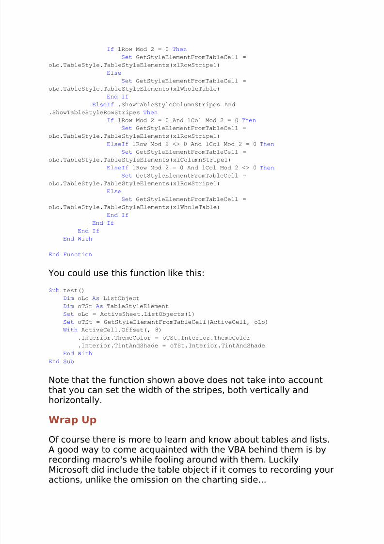
End Function

 You could use this function like this:

Sub test()

  Dim oLo As ListObject

  Dim oTSt As TableStyleElement

  Set oLo = ActiveSheet.ListObjects(1)

  Set oTSt = GetStyleElementFromTableCell(ActiveCell, oLo)

  With ActiveCell.Offset(, 8)

.Interior.ThemeColor = oTSt.Interior.ThemeColor

.Interior.TintAndShade = oTSt.Interior.TintAndShade

  End With

End Sub

Note that the function shown above does not take into accountthat you can set the width of the stripes, both vertically andhorizontally.

Wrap Up

Of course there is more to learn and know about tables and lists.A good way to come acquainted with the VBA behind them is byrecording macro's while fooling around with them. LuckilyMicrosoft did include the table object if it comes to recording youractions, unlike the omission on the charting side...

 

Custom Find

Deze pagina in het Nederlands

 

Finding Cells Matching A SpecificProperty Using The CallByNameFunction

Introduction

I thought it would be nice to have a generic VBA function to whichwe could pass a range object, a string indicating a property of theobject and the property's value, which would then return all cellsmatching that criteria.

CallByName

I decided it was time to explore the CallByName function,introduced with Office 2000. According to Excel XP VBA Help:

CallByName Function

Executes a method of an object, or sets or returns a property of an object.

Syntax

CallByName(object, procname, calltype,[args()])

 The CallByName function syntax has these named arguments:

Part Description

object Required; Variant (Object). The name of the object on which the

function will be executed.

procna

me

Required; Variant (String). A string expression containing the name of a

property or method of the object.

calltype Required; Constant. A constant of type vbCallType representing the

type of procedure being called. Can be vbGet (to return a property),

vbLet (to change a property), vbMethod (to execute a method) or vbSet

(to set an Object)

 

args() Optional: Variant (Array).

Suppose we'd want to find out the colorindex of a cell's interior:

Sub test()

MsgBox CallByName(ActiveCell.Interior, "Colorindex", VbGet)

End Sub

Since I would like to make this method a bit more general, I wouldlike to just pass the cell object and the entire "procname" in astring:

Sub test()

MsgBox CallByName(ActiveCell, "Interior.Colorindex", VbGet)

End Sub

Unfortunately, this does not work, "procname" only accepts asingle entity (Property, Method or Object). So it is necessary tosplit up the "procname" string into it's individual elements.

Something like this (note: Excel 97 doesn't have the Splitfunction, nor the CallByName function):

Dim lProps As Long

Dim vProps As Variant

vProps = Split(sProperties, ".")

lProps = UBound(vProps)

So to get at the colorindex property of the Interior object of theCell object, we need to loop through the variant vProps:

For lCount = 0 To lProps - 1

Set oTemp = CallByName(oTemp, vProps(lCount), VbGet)

Next

We stop the loop at the one-but-last element of vProps, becauseall of the elements except the last one will be objects and the lastone will be the property we're interested in. Then we get theproperty of the last object the loop has given us:

CallByName(oTemp, vProps(lProps), VbGet)

 The complete function is shown below:

Function FindCells(ByRef oRange As Range, ByVal sProperties As Strin

g, _

 

  ByVal vValue As Variant) As Range

  Dim oResultRange As Range

  Dim oArea As Range

  Dim oCell As Range

  Dim bDoneOne As Boolean

  Dim oTemp As Object

  Dim lCount As Long

  Dim lProps As Long

  Dim vProps As Variant

vProps = Split(sProperties, ".")

lProps = UBound(vProps)

  For Each oArea In oRange.Areas

  For Each oCell In oArea.Cells

  Set oTemp = oCell

  For lCount = 0 To lProps - 1

  Set oTemp = CallByName(oTemp, vProps(lCount), VbGet)

  Next

  If CallByName(oTemp, vProps(lProps), VbGet) =

vValue Then

  If bDoneOne Then

  Set oResultRange = Union(oResultRange, oCell)

  Else

  Set oResultRange = oCell

bDoneOne = True

  End If

  End If

  Next

  Next

  If Not oResultRange Is Nothing Then

  Set FindCells = oResultRange

  End If

End Function

A small example of its use, selecting all cells with a white fill:

Sub UseFindCellsExample()

FindCells(ActiveSheet.UsedRange, "Interior.ColorIndex",

0).Select

End Sub