Characterization of regimes and regime transitions …alexandria.tue.nl/repository/freearticles/617778.pdfCharacterization of regimes and regime transitions in bubble columns by chaos

Pergamon ('h,,mi~d E~oincerin,i Scieme, Vol. 52. N~. 24, pp. 4447 4459, I997 I 1997 Elsevier Science Ltd. All rights reserved

Printed in Great Britain PII: S0009-2509(97)00290-X o009 250997 $1700 + 0.00

Characterization of regimes and regime transitions in bubble columns by chaos

analysis of pressure signals

H. M. Letzel, **~ J. C. Schouten,* R. Krishna,* C. M. van den Bleek* *Delft University of Technology, Faculty of Chemical Technology, Julianalaan 136, 2628 BL

Delft, The Netherlands; +University of Amsterdam, Department of Chemical Engineering, Nieuwe Achtergracht 166, 1018 WV Amsterdam, The Netherlands

(Received 3 June 19961

Abstract - I n this study it is shown that the transition from the homogeneous to the heterogeneous flow regime in bubble columns can be quantitatively found with high accuracy by analysing the chaotic characteristics of the pressure fluctuation signal (PESt. In previous work (van den Bleek and Schouten, 1993; Schouten et al., 1996), the authors have already applied this technique to time series from gas-solid fluid beds. Also, it was shown (Krishna et al.. 1993, Ellenberger and Krishna, 1994) that hydrodynamics of bubble columns and fluid beds can be de~ribed in an analogous manner. Therefore in this work, the method of chaos analysis is applied to bubble columns. A distinctive feature of the pressure signal from bubble columns is that it is composed of two different parts: a low frequency part resulting from the motion of the large bubbles and a high frequency part resulting from all other processes (coalescence, collapse, breakup) that take place in the column. From the phase of the cross spectrum of two pressure probes, placed at different axial positions, it was possible to identify' the bands in the spectrum of the PFS that show a significant time delay. This time delay is of the order of the passage time of bubbles between the measurement locations. This band in the spectrum of the PFS was used to estimate the Kolmogorov entropy to quantify the chaotic dynamics in the bubble column. The Kolmogorov entropy as a function of gas velocity indicates a sharp transition from the homogeneous to the churn turbulent flow regime. From other methods considered (e.g. holdup and other properties of the signal such as variance), this transition was less clear. Therefore chaos analysis of PFSs is believed to be a powerful technique for on-line identification of flow regimes. C 1997 Elsevier Science Ltd

K e y w o r d s : Bubble column; flow regime transition: regime characterization: pressure sensing: chaos analysis: Kolmogorov entropy.

I N T R O D U C T I O N

For lnodelling and design of bubble column reactors, it is of great importance to know the flow regime or flow pattern. The reason is that a reactor model that is formulated for a specific flow regime is often not valid in a different flow regime due to different mass transfer, heat transfer and mixing characteristics. As an illustration of such a situation, a cold flow model of a bubble column reactor at ambient pressure can be considered: the flow regime prevailing in the pilot plant or in the commercial reactor to be built can differ considerably from that in the cold model, due to higher pressures (see, e.g. Tarmy et al., 1984). There-

:Corresponding author. Fax: + +31 15 2784452: e-mail: lelzel(u,st m.t udelft.nl.

fore the effects of pressure on the hydrodynamics in general and on the flow regime in particular need to be known. To study these pressure effects, an objective and accurate measurement technique is needed to identify the different regimes and the transitions between these.

An attractive option to study the hydrodynamics of bubble columns is the analysis of pressure fluctuations. The measuring method is well developed and relatively cheap. Furthermore, it is robust and therefore has great possibilities for use at industrial conditions, e.g. for "flow regime monitoring" as a part of process monitoring. Analysis of pressure fluctuations also has advantages compared to visual observation; objective, quantitative criteria for the flow regimes and flow regime transitions can be formulated. Furthermore, in high pressure experimental set ups or in industrial installations, visual observation is in many cases limited if not impossible.

4447

4448

In spite of its experimental advantages, analysis of pressure fluctuations is complicated; it is difficult to unravel from the measured signals the flow-regime characteristics. The reason is obvious: the processes that cause the pressure fluctuations (such as flow circulations and passage of bubbles) take place throughout the column; they are however 'projected' on a one-dimensional pressure signal. Unavoidably, information is hidden or lost in this way. Many authors however have shown that still relevant information about the flow can be obtained by analysis of the pressure fluctuation signal (PFS) by applying the appropriate signal processing techniques.

Examples of different signal processing techniques are (i) analyses of variance and Fourier spectra (Fan e ta l . , 1986), (ii) Hurst analysis or R/S analysis (Drahog et al., 1992; Fan et al., 1990), (iii) wavelet transformation and similar techniques, determining the instantaneous frequency. This technique was used by Bakshi et al. (1995), based on a gas holdup signal, and by Hervieu and Seleghim (1995), based on a pressure signal. The aim is to 'distill' more information about the hydrodynamics, by processing a representative signal from the bubble column with new methods.

In recent years, the hydrodynamic behaviour of gas-solid fluidized beds has been studied by considering it as a chaotic system. Van den Bleek and Schouten (1993), Schouten et al. (1996), Daw et al.

(1990) and Daw and Halow (1991) used the pressure signal to calculate chaotic invariants that characterize the system. Examples of such invariants are correlation dimension and Kolmogorov entropy. Krishna e ta l . (1993) and Ellenberger and Krishna (1994) showed that hydrodynamics in bubble columns are in many aspects analogous to that in gas-solid fluidized beds. Therefore, it is to be expected that bubble columns show comparable chaotic characteristics as fluidized beds.

In this work, the chaos analysis techniques as described by Van den Bleek and Schouten (1993) are applied to the analysis of pressure fluctuations in bubble columns. It will be shown that the transition from the homogeneous to the heterogeneous flow regime can be determined with high accuracy. Before the chaos analysis method can be applied, the signal needs to be pre-processed. Whereas in a gas-solid fluid bed the PFS is mainly due to bubbles, in a gas-liquid bubble column many more effects are present; with cross-spectral techniques, frequency bands containing these effects are identified and filtered out.

First, the principles of the chaos analysis method that is used, are described. Next, the analogies between gas-solid and gas-liquid flow are discussed, sketching at the same time the problems encountered in applying chaos analysis to the 'raw' pressure signal in gas-liquid flow. After description of the experimental set-up, the pre-processing of the signals is discussed. The obtained results are presented, and we end with conclusions and suggestions for applications and future work.

H. M. Letzel et al.

Bubble columns figure prominently in the research interest profile of Prof. M.M. Sharma as witnessed in his recent review (Sharma, 1993). Professor Sharma has always encouraged new concepts and ideas and it is a great pleasure for the authors to offer the current contribution as a tribute to him on his sixtieth birth- day.

CHAOS ANALYSIS OF PRESSURE SIGNALS

For an overview of the analysis of time series with chaotic characteristics, the reader is referred to Grass- berger et al. (1991). Below, some concepts of chaotic time series analysis will be introduced.

Chaot ic sys tem A chaotic system is a non-linear, deterministic sys-

tem that is extremely sensitive to small changes in initial conditions. Two initial states of the system that are almost identical will, after some time, develop in completely different ways. The reason is that the (very small) initial differences grow exponentially with time. The rate at which these differences grow, is a characteristic for the system. Limiting cases are zero growth: a completely ordered system, and infinitely fast growth: a stochastic system. The rate of growth of the difference between two initial conditions in time is expressed in quantities like Lyapunov exponents and Kolmogorov entropy; these quantify the unpredictability of the system.

A t t r a c t o r

It is possible to represent any physical system by a plot in its s tate space; this is an imaginary space with m axes, each representing a state variable of the system. Every state of the system now corresponds to a point in the state space. The co-ordinate values for this point are equal to the values of the corresponding state variables.

As an example a pendulum is considered. The two state variables are angle and angular velocity. Plot- ting these quantities in a two-dimensional state space, the plot in Fig. 1 is obtained. The curves in the plots, representing the states of the system at consecutive time steps are called trajectories or orbits. The part of the state space to which the trajectories converge is called the at t rac tor of the system; in case of a pendulum this can be a single point (damped pendulum: A) or a limit cycle (undamped pendulum: B). These at- tractors are finite. This is a characteristic for fully predictable systems.

Consider now the attractor for say a gas-solid fluidized bed. In this case, the attractor has a dimension higher than unity, whereas only a limited number of signals are available to reconstruct the attractor from, e.g. pressure and/or porosity. However, it was shown by Takens (1981), that it is possible to reconstruct an m-dimensional state space plot by means of only one characteristic variable, using the method of delay co-ordinates: the values of the variable at different time delays (0, At, 2At . . . . . (m -- 1)At) are used as

Characterization of regimes in bubble columns

co-ordinate values in the 'embedding space'. Takens (1981) proved that the state space plot obtained in this way in principle shows the same dynamics and chaotic characteristics as the state space plot that would have been obtained if all the state variables would have been used as co-ordinate values.

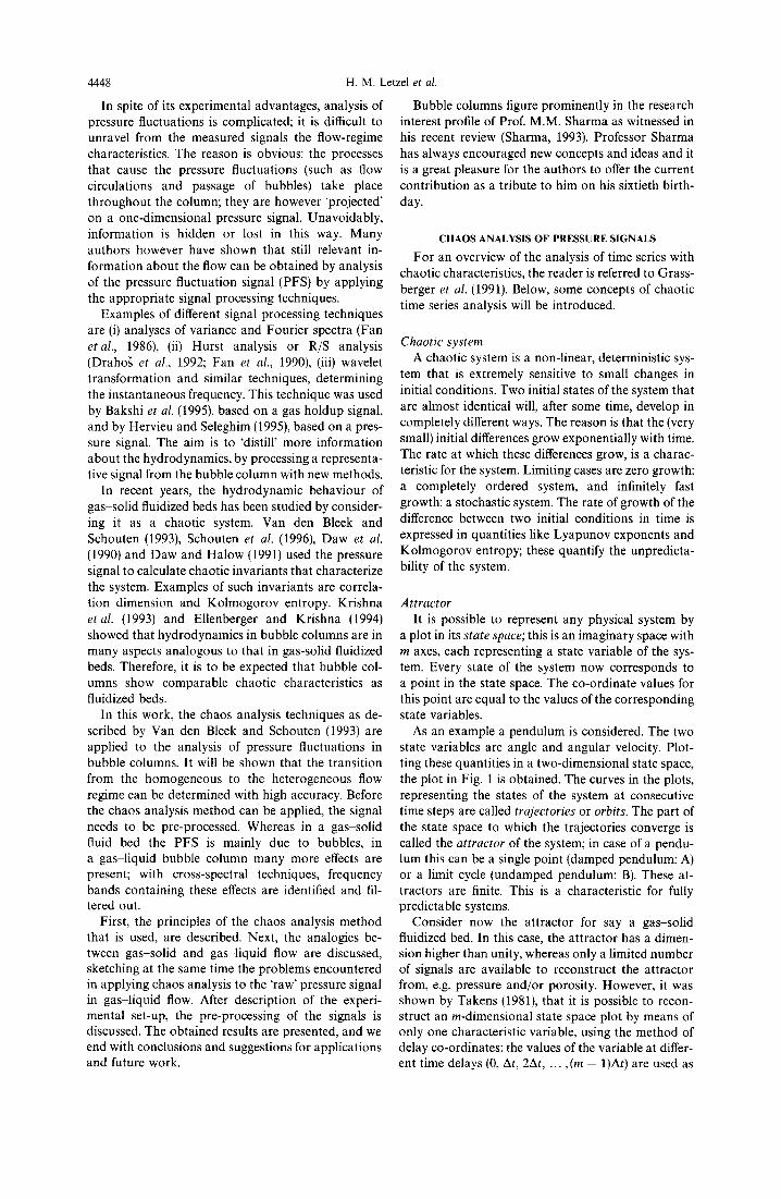
Figure 2 shows a 2D projection of a higher dimensional state space plot from a pressure fluctuation time series, measured in a fluidized bed (38.4 cm inner diameter, 400/~m sand particles, U o = 0.24 m/s). The non-finite attractor obtained in this way is a strange attractor, a typical feature of a chaotic system. For a chaotic system, the strange attractor has a finite dimension that is smaller than the dimension of the embedding space (if the latter is chosen sufficiently high). This dimension, which can be a non-integer, is called the fractal dimension.

j f,0

CO

D A: d a m p ~ ~ ~ _ 0

B: undam~[~ 0

Fig. 1. Plot of state of a pendulum in state space for a damped pendulum (point attractor: A) and an undamped

pendulum (limit cycle: B).

4449

Kolmogorov entropy Systems with a strange attractor have a limited

predictability. The degree of predictability however varies according to the system. Limiting cases are completely predictable systems, like the undamped pendulum, and completely unpredictable systems: stochastic systems. The predictability can be quantified as follows. Consider two nearby points that lie on different orbits of the attractor. These points represent two states of the system, separated in time, with almost equal conditions. The rate at which the orbits separate expresses the 'degree of unpredictability'. It is quantified by the Kolmogorov entropy, a characteristic invariant proportional to the rate of separation of two orbits. Schouten et al. (1994a) and Schouten and Van den Bleek (1992-1995) developed methods and software for a maximum likelihood estimation of the Kolmogorov entropy. The correlation dimension is calculated using the maximum likelihood estimation of Takens as described by Schouten et al. (1994bl.

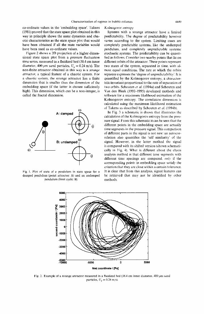
In Fig. 3 a schematic is drawn that illustrates the calculation of the Kolmogorov entropy from the pressure signal. From this schematic it can be seen that the different points in the embedding space are actually time segments in the pressure signal. This comparison of different parts in the signal is not new: an autocor- relation also quantifies the 'self similarity' of the signal. However, in the latter method the signal is compared with its shifted version (shown schemati- cally in Fig. 4). What is different about the chaos analysis method is that different time segments with different time spacings are compared, only if the corresponding points in embedding space satisfy the criterion that they are close within a certain tolerance. It is clear that from this analysis, signal features can be retrieved that may not be identified by other methods.

5000 / 4000 I

L I

-1ooo I "2000 I "3000 I

-10000 ~000 0 5000 first coordinate I [Pa]

Fig. 2. Example of a strange attractor measured in a fluidized bed (38.4 cm inner diameter. 400 #m sand particles, U s = 0.24 m/s).

4450 H. M. Letzel etal.

m samples

AI-: A • I I I I I

^ ~ hA~ ^'A~AA^'M,.

I.~.a I V . . , { _ ~ I p J

vectors in m-dimensional ', m - dimensional attractor space

Rate of separation: unpredictability, quantified by Kolmogorov entropy

Fig. 3. Schematic of the calculation method for Kol- mogorov entropy from the time series of one variable: if two time segments are close in state space, their future is com-

pared.

homogeneous : Ug

Ut rans

£

i U0 Ut rans

large l bubbles small bubbles

heterogeneous

bubbles dense phase

Fig. 5. Analogy concept of Krishna et al. (1993): gas-liquid flow (above) and gas solid flow {below) consist of a dense phase (small bubbles respectively emulsion phase) and a di-

lute phase (large bubbles).

Pll I i V VV VX/Vv ' VVV v V': t

a :

!: V VVV v v,Vl

R12(a)= J'Pl(t)Pz(t+a) dt

Fig. 4. Schematic of calculation method for cross correlation: the entire signal is compared with a shifted version of

itself.

ANALOGY BETWEEN FLUID BEDS AND BUBBLE

COLUMNS

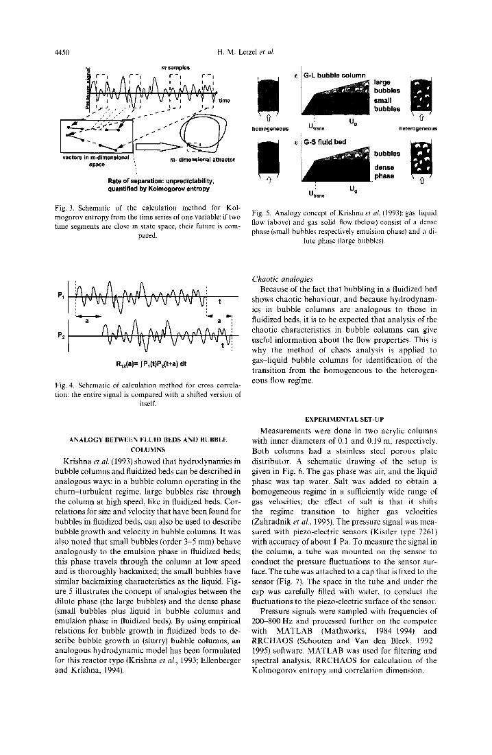
Krishna et al. (1993) showed that hydrodynamics in bubble columns and fluidized beds can be described in analogous ways: in a bubble column operating in the churn turbulent regime, large bubbles rise through the column at high speed, like in fluidized beds. Cor- relations for size and velocity that have been found for bubbles in fluidized beds, can also be used to describe bubble growth and velocity in bubble columns. It was also noted that small bubbles (order 3-5 mm) behave analogously to the emulsion phase in fluidized beds; this phase travels through the column at low speed and is thoroughly backmixed; the small bubbles have similar backmixing characteristics as the liquid. Fig- ure 5 illustrates the concept of analogies between the dilute phase (the large bubbles) and the dense phase (small bubbles plus liquid in bubble columns and emulsion phase in fluidized beds). By using empirical relations for bubble growth in fluidized beds to describe bubble growth in (slurry) bubble columns, an analogous hydrodynamic model has been formulated for this reactor type (Krishna etal . , 1993; Ellenberger and Krishna, 1994).

Chaotic analogies Because of the fact that bubbling in a fluidized bed

shows chaotic behaviour, and because hydrodynamics in bubble columns are analogous to those in fluidized beds, it is to be expected that analysis of the chaotic characteristics in bubble columns can give useful information about the flow properties. This is why the method of chaos analysis is applied to gas-liquid bubble columns for identification of the transition from the homogeneous to the heterogeneous flow regime.

EXPERIMENTAL SET-UP

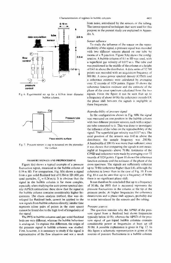
Measurements were done in two acrylic columns with inner diameters of 0.1 and 0.19 m, respectively. Both columns had a stainless steel porous plate distributor. A schematic drawing of the setup is given in Fig. 6. The gas phase was air, and the liquid phase was tap water. Salt was added to obtain a homogeneous regime in a sufficiently wide range of gas velocities; the effect of salt is that it shifts the regime transition to higher gas velocities (Zahradnik et al., 1995). The pressure signal was measured with piezo-electric sensors (Kistler type 7261) with accuracy of about 1 Pa. To measure the signal in the column, a tube was mounted on the sensor to conduct the pressure fluctuations to the sensor surface. The tube was attached to a cap that is fixed to the sensor (Fig. 7). The space in the tube and under the cap was carefully filled with water, to conduct the fluctuations to the piezo-electric surface of the sensor.

Pressure signals were sampled with frequencies of 200-800 Hz and processed further on the computer with MATLAB (Mathworks, 1984-1994) and RRCHAOS (Schouten and Van den Bleek, 1992 1995) software. MATLAB was used for filtering and spectral analysis, RRCHAOS for calculation of the Kolmogorov entropy and correlation dimension.

tu be data acquisition \

/ sensor :.

Q__

control

- - e pressure control


0.19 m

A

2.0 m

!

2.0 m

Fig. 6. Experimental set up for a 0.19m inner diameter bubble column.

4451

from noise, introduced by the sensors or the tubing. The (cross) spectral techniques that were used for this purpose in the present study are explained in Appen- dix A.

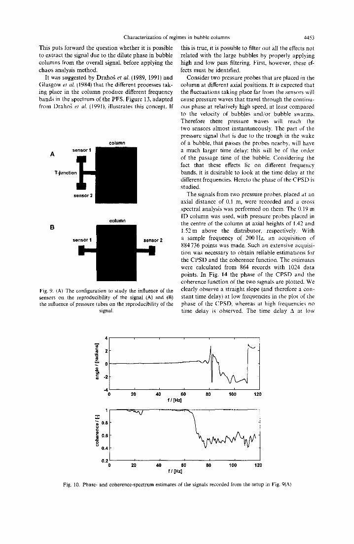
Sensor influence To study the influence of the sensor on the repro-

ducibility of the signal, a pressure signal was recorded with two different sensors placed on one tube by means of a T-junction. Figure 9(A) shows the configuration. A bubble column of 0.1 m ID was used, with a superficial gas velocity of 0.077 m/s. The tube end was positioned in the middle of the column at a height of 0.43 m above the distributor. A data series of 32 768 points was recorded with an acquisition frequency of 800 Hz. A cross power spectral density (CPSD) and a coherence estimate were calculated by averaging over 32 records of 1024 points. Figure 10 shows the coherence function estimate and the estimate of the phase of the cross spectrum calculated from the two signals. From the figure it can be seen that up to a frequency of about 64 Hz the coherence exceeds 0.9; the phase shift between the signals is negligible at these frequencies.

vvv, Cap

vvv'

Piezo electric surface

Pressure tube

I

Fig. 7. Pressure sensor: a cap is mounted on the piezoelec- tric surface.

PRESSURE SIGNALS AND PREPROCESSING

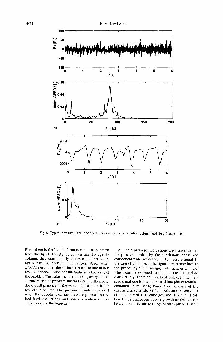
Figure 8(a) shows a typical example of a pressure fluctuation signal, measured in the bubble column of 0.19 m |D. For comparison, Fig. 8(b) shows a signal from a gas-solid fluidized bed of 0.384 m ID (400/~m sand particles, U 0 = 0.24 m/s). It is obvious that the signal in the bubble column is far more complex, especially when studying the auto power spectral density (APSD) estimations: these show that the signal in the bubble column contains considerably higher frequencies. The chaos analysis method, that was developed for fluidized beds, cannot be applied to the raw signals from bubble columns directly; similar time segments (close pairs of points in the state space) cannot be found due to the high level of irregularity of the signal.

The PFS in bubble columns and gas-solid fluidized beds are very different, whereas the bubble behaviour is analogous. To explain this difference, the origin of the pressure signal in bubble columns was studied. First, however, it is necessary to study if the signal is representative of the flow situation and not a result

Reproducibility of pressure signal In the configuration shown in Fig. 9(B) the signal

was measured on one position in the bubble column with two different pressure sensors, each with a separate tube connected to it. This was done to investigate the influence of the tubes on the reproducibility of the signal. The superficial gas velocity was 0.117 m/s. The axial position of the sensors was 0.43 m above the distributor, the sample frequency was 200 Hz. A bandwidth of 100 Hz was more than sufficient, since it was shown that comparing the signals is not mean- ingful at frequencies above 70 Hz. Estimates of the CPSD and coherence were made by averaging over 32 records of 1024 points. Figure 11 shows the coherence function estimate and the estimate of the phase of the cross spectrum. The signals are sufficiently coherent up to 70 Hz (coherence higher than 0.8), although the coherence is lower than in the case of Fig. 10. From Fig. 11 it can be seen that up to a frequency of 50 Hz there is no significant phase shift.

It can therefore be concluded that up to a frequency of 50 Hz, the PFS that is measured represents the pressure fluctuations in the column at the tip of the pressure probe. At higher frequencies the coherency deteriorates and a phase shift appears, probably due to noise introduced by the sensors and the tubing.

Pressure sources The question remains why the APSD of the pres-

sure signal from a fluidized bed shows frequencies typically below 10 Hz, whereas the APSD of the pressure signal of gas-liquid bubble columns contains considerable power at frequencies at least up till 50 Hz. A possible explanation is given in Fig. 12. In this figure a schematic representation is given of the sources of pressure iluctuations in a bubble column.

4452 H.M. Letzel et al.

100

" 50 D.

0

-50

-100 0

,-;, 0.06

7,

o. 0.04 ,<

o 0.02

(a)

1 2 3 4 5 6 t/[s]

i I I

50 100 150 200

f / [ H ~

2000

0

-2000

1

7`

< 0.5

O

0 0

(b)

I I I I I

I I I I l

1 2 3 4 5 6 t / [s]

5 10 15 20 f / [Hzl

Fig. 8. Typical pressure signal and spectrum estimate for (a) a bubble column and {b) a fluidized bed.

First, there is the bubble formation and detachment from the distributor. As the bubbles rise through the column, they continuously coalesce and break up, again causing pressure fluctuations. Also, when a bubble erupts at the surface a pressure fluctuation results. Another source for fluctuations is the wake of the bubbles. The wake oscillates, making every bubble a transmitter of pressure fluctuations. Furthermore, the overall pressure in the wake is lower than in the rest of the column. This pressure trough is observed when the bubbles pass the pressure probes nearby. Bed level oscillations and macro circulations also cause pressure fluctuations.

All these pressure fluctuations are transmitted to the pressure probes by the continuous phase and consequently are noticeable in the pressure signal. In the case of a fluid bed, the signals are transmitted to the probes by the suspension of particles in fluid, which can be expected to dampen the fluctuations considerably. Therefore in a fluid bed, only the pressure signal due to the bubbles (dilute phase) remains. Schouten et al. (1996) based their analysis of the chaotic characteristics of fluid beds on the behaviour of these bubbles. Ellenberger and Krishna (1994) based their analogous bubble growth models on the behaviour of the dilute (large bubble) phase as well.


This puts forward the question whether it is possible to extract the signal due to the dilute phase in bubble columns from the overall signal, before applying the chaos analysis method.

It was suggested by Draho~ et al. (1989, 1991) and Glasgow et al. (1984) that the different processes taking place in the column produce different frequency bands in the spectrum of the PFS. Figure 13, adapted from Draho~ et al. (1991), illustrates this concept. If

A

column

T-junctior

B column

Fig. 9. (A) The configuration to study the influence of the sensors on the reproducibility of the signal (A) and (B) the influence of pressure tubes on the reproducibility of the

signal.

4453

this is true, it is possible to filter out all the effects not related with the large bubbles by properly applying high and low pass filtering. First, however, these effects must be identified.

Consider two pressure probes that are placed in the column at different axial positions. It is expected that the fluctuations taking place far from the sensors will cause pressure waves that travel through the continuous phase at relatively high speed, at least compared to the velocity of bubbles and/or bubble swarms. Therefore these pressure waves will reach the two sensors almost instantaneously. The part of the pressure signal that is due to the trough in the wake of a bubble, that passes the probes nearby, will have a much larger time delay; this will be of the order of the passage time of the bubble. Considering the fact that these effects lie on different frequency bands, it is desirable to look at the time delay at the different frequencies. Hereto the phase of the CPSD is studied.

The signals from two pressure probes, placed at an axial distance of 0.1 m, were recorded and a cross spectral analysis was performed on them. The 0.19 m ID column was used, with pressure probes placed in the centre of the column at axial heights of 1.42 and 1.52m above the distributor, respectively. With a sample frequency of 200 Hz, an acquisition of 884 736 points was made. Such an extensive acquisition was necessary to obtain reliable estimations for the CPSD and the coherence function. The estimates were calculated from 864 records with 1024 data points. In Fig. 14 the phase of the CPSD and the coherence function of the two signals are plotted. We clearly observe a straight slope (and therefore a constant time delay) at low frequencies in the plot of the phase of the CPSD, whereas at high frequencies no time delay is observed. The time delay A at low

4

.I 2

0

O ~

~= -2

- 4 i i

0 20 40

1

~0.8

0.6 / -

O o

0.4

0.2

- ' ' x /

i i i J

I I I

60 80 100 120 f / [Hzl

i

i i i I i

20 40 60 80 100 120 f / W z l

Fig. 10. Phase- and coherence-spectrum estimates of the signals recorded from the setup in Fig. 9(A).

4454 H.M. Letzel et al.

0.5 t ~

0

"~ -0.5 i -

e= -1

-1.5 0

1 , " i "

~uO.8 e - .= o 0.6 o

i i i i

I I I I

20 40 60 80 f / [Hz]

100

0.4 i i i I

0 20 40 60 80 100 f I [Hz]

Fig. 11. Phase- and coherence spectrum estimates of the signals recorded from the setup in Fig. 9(B).

bed level o s c i l l a t i o n s . ~ bubble erupti¢

pressure trou~

breakup I coales

Bubble I Turbulence] Columnsl IcirculaUon Bubbles

I I I I ensor 1 10-1 100 101 102

Frequency (Hz) ensor 2

bubble formati

t.A

Fig. 12. Schematic representation of the sources of the pressure fluctuations in gas liquid flow.

frequencies is estimated from the slope of the phase spectrum:

6qo 2~t - - = 2 n A ~ - - . 6f 6

This gives a time delay of about i s which corresponds to a velocity of 0.6 m/s, The estimation of large bubble velocity with data from Ellenberger and Krishna (1994), given in Appendix B, shows that this velocity is of the order of the rise velocity is of the large bubbles: V~ ~ 0.6 m/s.

If the probe distance doubles, the time spacing should double, assuming the same bubble velocities. In Fig. 15 the phase of the CPSD and the coherence function are depicted, resulting from a probe spacing of 0.2 m. The slope has doubled, indicating a double time delay:

&p 2n - - = 2 ~ A ~ - 6f 3

Fig. 13. Location of different pressure fluctuation sources on the spectrum (from Draho~ et al. 1991)

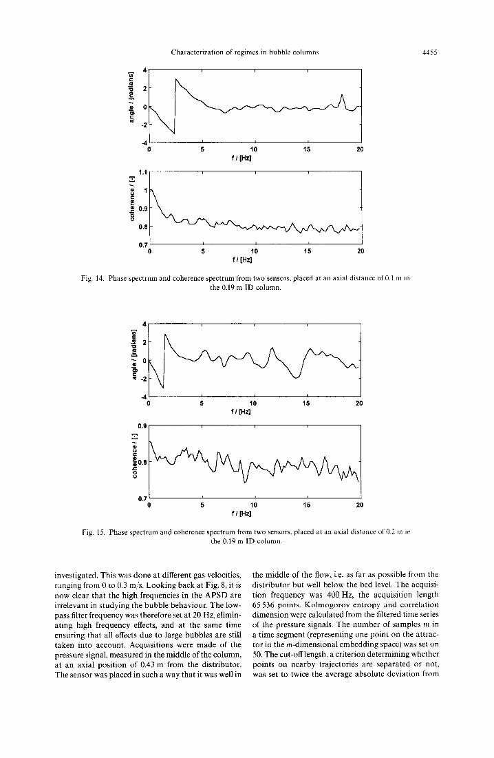
which corresponds to the same velocity of the bubble, i.e. Vh ~ 0.6 m/s. For the higher frequencies we see from Fig, 14 that there is no time shift. It is therefore concluded that the signal due to large bubbles can be found in the low frequency range, typically below 10 Hz. The estimation of the phase of the CPSD seems less reliable, but this can be expected because the probes lie too far apart for the small fluctuations to be coherent.

From Fig. 14 it is concluded that the bubble dynamics are represented by the low frequencies (1 10 Hz) of the spectrum of the pressure fluctuations. Pressure fluctuations due to macro circulations of the fluid in the bubble column and due to bed level oscillations are expected to lie on a much lower frequency, of order 10 1 Hz (Draho~ and Cerm/tk, 1989).

Summarizing, we state that not only large bubbles, but many more effects contribute to the unfiltered PFS. The low-dimensional, chaotic behaviour of bubble columns, that is assumed to result from the large bubble behaviour, can be studied by looking at the low-frequency-part of the spectrum.

REGIME TRANSITION

To determine the regime transition, the chaotic properties of the low-frequency-part of the PFS were

Characterization of regimes in bubble columns 4455

W e -

.-.R "O

@ O~ e-

2

0

-2

..4.

1.1

0 e -

0.9 O o

0.8

0.7 0

I i i

5 10 15 20 f / [Hz]

I I i

5 10 15 20 f ! [Hz]

Fig. 14. Phase spectrum and coherence spectrum from two sensors, placed at an axial distance of 0.1 in in the 0.19 m ID column.

4 W

0

-2

-4

i i I

I I I

0 5 10 15 20 f I [Hz]

0.9

~0.8 c - o o

0.7 0 5 10 15 20

f t [Hz]

Fig. 15. Phase spectrum and coherence spectrum from two sensors, placed at an axial distance of 0.2 m in the 0.19 m ID column.

investigated. This was done at different gas velocities, ranging from 0 to 0.3 m/s. Looking back at Fig. 8, it is now clear tha t the h igh frequencies in the A P S D are i rrelevant in s tudying the bubble behaviour . The low- pass filter frequency was therefore set at 20 Hz, elimin- at ing high frequency effects, and at the same time ensur ing tha t all effects due to large bubbles are still taken into account. Acquisi t ions were made of the pressure signal, measured in the middle of the column, at an axial posi t ion of 0.43 m from the distr ibutor . The sensor was placed in such a way tha t it was well in

the middle of the flow, i.e. as far as possible from the d is t r ibutor but well below the bed level. The acquisi- t ion frequency was 400 Hz, the acquisi t ion length 65 536 points. K o l m o g o r o v en t ropy and corre la t ion d imens ion were calculated from the filtered time series of the pressure signals. The n u m b e r of samples m in a t ime segment (representing one point on the at trac- tor in the m-dimensional embedd ing space) was set on 50. The cut-off length, a cri terion de termining whether points on nearby trajectories are separated or not, was set to twice the average absolute devia t ion from

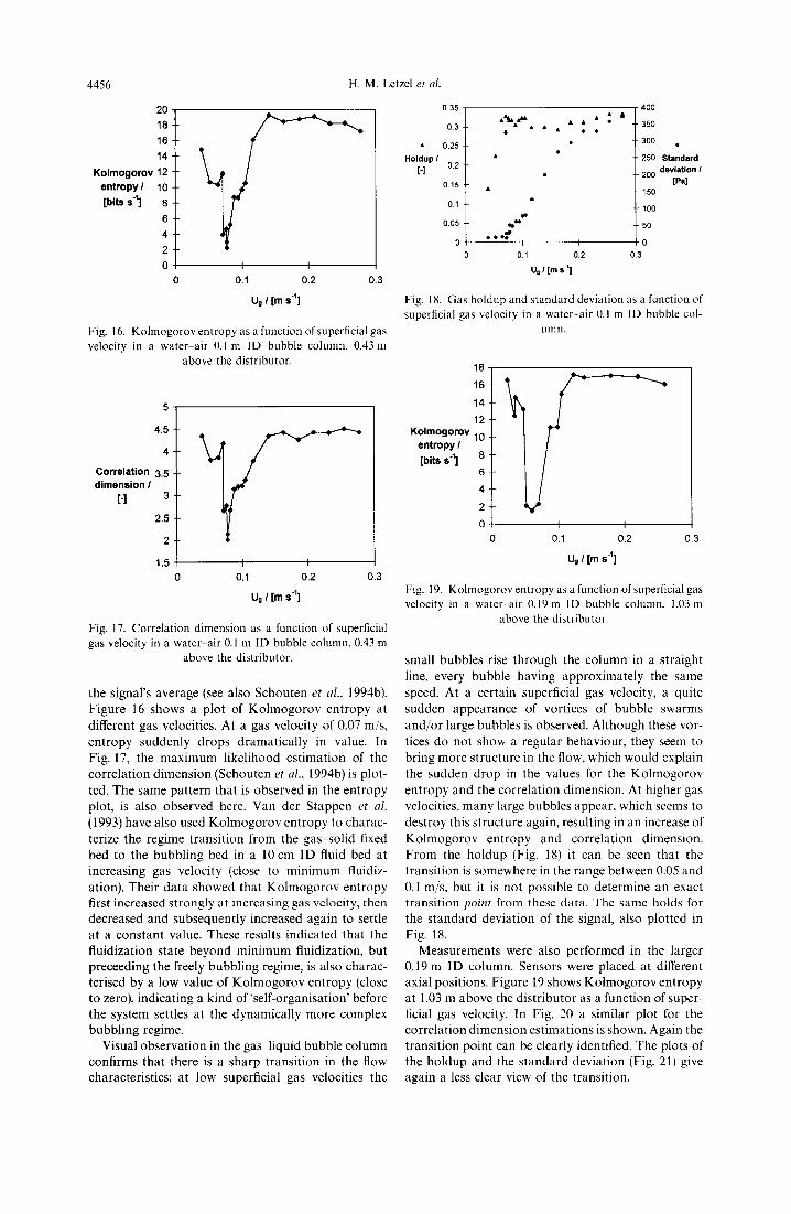
4456 H. M. Letzel eta/.

20 18 16

14

Kolmogorov 12 entropyl 10 [bits s"] 8

6

4 2

0 0 0.1 0.2 0.3

Ug / [m s "1]

Fig. 16. Kolmogorov entropy as a function of superficial gas velocity in a water air 0.l m ID bubble column, 0.43 in

above the distributor.

5

4.5

4

Correlation 3.5 dimension /

[-I 3

2.5

2 '

1.5

I I

I I 0.1 0.2 0.3

Ug / [m s "1]

Fig. 17. Correlation dimension as a function of superficial gas velocity in a water air 0.1 m ID bubble column, 0.43 m


the signal's average (see also Schouten et al., 1994b). Figure 16 shows a plot of Kolmogorov entropy at different gas velocities. At a gas velocity of 0.07 m/s, entropy suddenly drops dramatically in value. In Fig. 17, the maximum likelihood estimation of the correlation dimension (Schouten et al., 1994b) is plotted. The same pattern that is observed in the entropy plot, is also observed here. Van der Stappen et al. (1993) have also used Kolmogorov entropy to characterize the regime transition from the gas solid fixed bed to the bubbling bed in a 10 cm ID fluid bed at increasing gas velocity (close to minimum fluidization). Their data showed that Kolmogorov entropy first increased strongly at increasing gas velocity, then decreased and subsequently increased again to settle at a constant value. These results indicated that the fluidization state beyond minimum fluidization, but preceeding the freely bubbling regime, is also charac- terised by a low value of Kolmogorov entropy (close to zero), indicating a kind of 'self-organisation' before the system settles at the dynamically more complex bubbling regime.

Visual observation in the gas liquid bubble column confirms that there is a sharp transition in the flow characteristics: at low superficial gas velocities the

Holdup I [-]

0,35

0.3

0.25

0.2

0.15

0.1

0.05

0

• • •

• e l • l0 I I

0.1 0.2

U. / [m $41

4 0 0

II 350

3O0

250 Standard deviation /

20O [Pa]

- 150

100

50

0

0.3

Fig. 18. Gas holdup and standard deviation as a function of superficial gas velocity in a water-air 0.! m ID bubble col-

umn.

Kolmogorov entropy / [bits s "1]

1 8

1 6

1 4

12'

10'

8

6

4

2

0 I I 0.1 0.2 0.3

Ug / [m s "1]

Fig. 19. Kolmogorov entropy as a function of superficial gas velocity in a water air 0.19 m ID bubble column, 1.03 m


small bubbles rise through the column in a straight line, every bubble having approximately the same speed. At a certain superficial gas velocity, a quite sudden appearance of vortices of bubble swarms and/or large bubbles is observed. Although these vortices do not show a regular behaviour, they seem to bring more structure in the flow, which would explain the sudden drop in the values for the Kolmogorov entropy and the correlation dimension. At higher gas velocities, many large bubbles appear, which seems to destroy this structure again, resulting in an increase of Kolmogorov entropy and correlation dimension. From the holdup (Fig. 18) it can be seen that the transition is somewhere in the range between 0.05 and 0.1 m/s, but it is not possible to determine an exact transition point from these data. The same holds for the standard deviation of the signal, also plotted in Fig. 18.

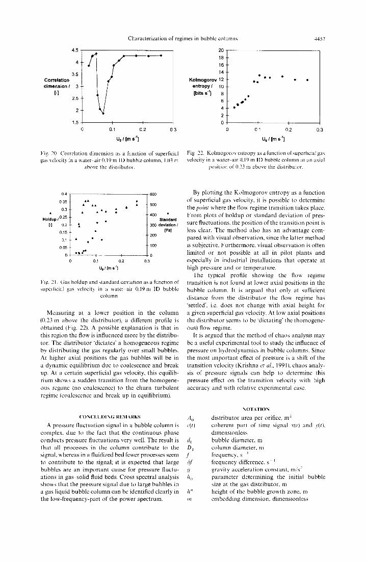
Measurements were also performed in the larger 0.19 m ID column. Sensors were placed at different axial positions. Figure 19 shows Kolmogorov entropy at 1.03 m above the distributor as a function of superficial gas velocity. In Fig. 20 a similar plot for the correlation dimension estimations is shown. Again the transition point can be clearly identified. The plots of the holdup and the standard deviation (Fig. 21) give again a less clear view of the transition.

I I

4.5

4

3.5

3

2.5

2

1.5

Corre la t ion d imens ion I

[ ' l


0.1 0.2 0.3

Ug I [m s'l]

20

18

16

14

K o l m o g o r o v 12 e n t r o p y / 10

[bits s -~] 8

6

4

2

0

e

o o

I I

4 4 5 7

0 0.1 0.2 0.3

Ug / [m s-~]

Fig. 20. Correlation dimension as a function of superficial gas velocity in a water air 0.19 m ID bubble column, 1.03 m


Fig. 22. Kolmogorov entropy as a function of superficial gas velocity in a water air 0.19 m 1D bubble column at an axial

position of 0.23 m above the distributor.

04

035

0.3

Holdup 10.25

[-I 0.2 015

01

005

0

A A& &&

, •

o4b • ° ° I I

0.1 0.2

U a I [m s -~]

600

~" 500

400 * Standard

300 deviation I [Pa]

200

100

0 0.3

Fig. 21. Gas holdup and standard deviation as a function of superficial gas velocity in a water air 0.19 m ID bubble

cohlmn.

Measuring at a lower position in the column (0.23 m above the distributor), a different profile is obtained (Fig. 22). A possible explanation is that in this region the flow is influenced more by the distributor. The distributor 'dictates' a homogeneous regime by distributing the gas regularly over small bubbles. At higher axial positions the gas bubbles will be in a dynamic equilibrium due to coalescence and break up. At a certain superficial gas velocity, this equilibrium shows a sudden transition from the homogeneous regime (no coalescence) to the churn turbulent regime (coalescence and break up in equilibrium).

C O N C L U D I N G R E M A R K S Ao

A pressure fluctuation signal in a bubble column is c(t) complex, due to the fact that the continuous phase conducts pressure fluctuations very well. The result is d b that all processes in the column contribute to the D T signal, whereas in a fluidized bed fewer processes seem .[ to contribute to the signal; it is expected that large ,~[ bubbles are an important cause for pressure fluctu- H ations in gas solid fluid beds. Cross spectral analysis h o shows that the pressure signal due to large bubbles in a gas liquid bubble column can be identified clearly in h* the low-frequency-part of the power spectrum, m

By plotting the Kolmogorov entropy as a function of superficial gas velocity, it is possible to determine the point where the flow regime transition takes place. From plots of holdup or standard deviation of pressure fluctuations, the position of the transition point is less clear. The method also has an advantage compared with visual observation, since the latter method is subjective. Furthermore, visual observation is often limited or not possible at all in pilot plants and especially in industrial installations that operate at high pressure a n d o r temperature.

The typical profile showing the flow regime transition is not found at lower axial positions in the bubble column. It is argued that only at sufficient distance from the distributor the flow regime has "settled', i.e. does not change with axial height for a given superficial gas velocity. At low axial positions the distributor seems to be 'dictating" the [homogeneous) flow regime.

It is argued that the method of chaos analysis may be a useful experimental tool to study the influence of pressure oll hydrodynamics in bubble columns. Since the most important effect of pressure is a shift of the transition velocity (Krishna et al., 1991 ), chaos analysis of pressure signals can help to determine this pressure effect on tile transition velocity with high accuracy and with rehttive experimental ease.

~ O T A T I O N

distributor area per orifice, m 2 coherent part of time signal xlt) and y(t), dimensionless bubble diameter, m column diameter, m frequency, s frequency difference, s gravity acceleration constant, m/s 2 parameter determining the initial bubble size at the gas distributor, m height of the bubble growth zone, m embedding dimension, dimensionless

4458

P t At

Udf Ug Wtrans Vb x(t) y(t)

H. M. Letzel et al.

pressure, Pa time, s characteristic time step in entropy calculation, s gas velocity through the dense phase, m/s superficial gas velocity, m/s superficial gas velocity at transition, m/s large bubble velocity, m/s time signal, dimensionless time signal, dimensionless

Greek letters proportionality constant in Darton relation, eq. (B1), dimensionless

A time delay between two signals, s e voidage, dimensionless el.z(t) non-coherent part of time signal x(t) and

y(t), dimensionless q5 phase, dimensionless

proportionality constant in Werther relation, eq. (B2), dimensionless

6~b phase difference, dimensionless

Abbreviations APSD Auto Power Spectral Density CCF Cross Correlation Function CPSD Cross Power Spectral Density PFS Pressure Fluctuation Signal

REFERENCES

Bakshi, B. R., Zhong, H., Jiang, P. and Fan, L. S. (1995) Analysis of flow in gas-liquid bubble columns using multi-resolution methods. Trans. Inst. Chem. Engrs 73, 608-614.

Darton, R. C., LaNauze, R. D., Davidson, J. F. and Harrison, D. (1977) Bubble growth due to coalescence in fluidized beds. Trans. Inst. Chem. Engrs 55, 274-280.

Daw, C. S. and Halow, J. S. (1991) Characterization of voidage and pressure signals from fluidized beds using deterministic chaos theory. Proceedings of the 11th International Conference On Fluidized Bed Combustion, ed. E. J. Anthony, Vol. 1, pp. 777-786.

Daw, C. S., Lawkins, W. F., Downing, D. J. and Clapp, N. E. (1990) Chaotic characteristics of a complex gas solid flow. Phys. Rev. A 41, 1179-1181.

Draho~, J., Bradka, F. and Puncochfir, M. (1992) Fractal behaviour of pressure fluctuations in a bubble column. Chem. Engng Sci. 47, 4069-4075.

Draho§, J. and Cermfik, J. (1989) Diagnostics of gas-liquid flow patterns in chemical engineering systems. Chem. Engng Process. 26, 147-164.

Draho~, J., Zahradnik, M., Puncochfir, M., Fialovfi, M. and Bradka, F. (1991) Effect of operating conditions on the characteristics of pressure fluctuations in a bubble column. Chem. Engng Process. 29, 107 115.

Ellenberger, J. and Krishna, R. (1994) A unified approach to the scale-up of gas-solid fluidized bed and gas-liquid bubble column reactors. Chem. Engng Sci. 49, 5391-5411.

Fan, L. T., Neogi, D., Yashima, M. and Nassar, R. (1990) Stochastic analysis of a three-phase fluidized bed: fractal approach. A.I.Ch.E.J. 36, 1529-1535.

Fan, L. S., Satija, S. and Wisecarver, K. (1986) Pres- sure fluctuation measurements and flow regime transitions in gasqiquid fluidized beds. A.I.Ch.E.J. 32, 338-340.

Glasgow, L. A., Erickson, L. E., Lee, C. H. and Patel, S. A. (1984) Wall pressure fluctuations and bubble size distributions at several positions in an airlift fermentor. Chem. Engng Commun. 29, 311-336.

Grassberger, P., Schreiber, Th. and Schraffrath, C. (1991) Nonlinear time sequence analysis, lnt. J. Bifurcation Chaos 1, 521-547.

Hervieu, E. and Seleghim Jr, P. (1995) Characteriza- tion of gas-liquid two-phase flow pattern transition by analysis of the instantaneous frequency. Pro- ceedings of the 2nd International conference on multiphaseflow, April 3-7 (1995) Kyoto, Japan.

Krishna, R., Ellenberger, J. and Hennephof, D. E. (1993) Analogous description of the hydrodynamics of gas-solid fluidized beds and bubble columns. Chem. Engng J. 53, 89-101.

Krishna, R., Wilkinson, P. M. and Van Dierendonck, L. L. (1991) A model for gas holdup in bubble columns incorporating the influence of gas density on flow regime transitions. Chem. Engng Sci. 46, 2491-2496.

Mathworks (1984-1994) MATLAB User Manual. The Mathworks inc., Natick, MA., U.S.

Schouten, J. C., Takens, F. and Van den Bleek, C. M. (1994a) Maximum-likelihood estimation of the entropy of an attractor. Phys. Rev. E 49, 126-129.

Schouten, J. C., Takens, F. and Van den Bleek, C. M. (1994b) Estimation of the dimension of a noisy attractor. Phys. Rev. E 50, 1851-1861.

Schouten, J. C. and Van den Bleek, C. M. (1992) A.I.Ch.E. Symp. Ser. 88, 70-84.

Schouten, J. C. and Van den Bleek, C. M. (1992-1995) RRCHAOS: an interactive software package for deterministic chaos analysis of non-linear time series. Reactor Research Foundation, Delft, The Netherlands.

Schouten, J. C., Vander Stappen, M. L. M. and Van den Bleek, C. M. (1996) Scale-up of chaotic fluidized bed hydrodynamics. Chem. Engng Sci. 51, 1991-2000.

Sharma, M. M. (1993) Some novel aspects of multi- phase reactions and reactors. Trans. lnstn. Chem. Engrs Part A 71, 595-610.

Takens, F. (1981) Lecture notes in Mathematics, Vol. 898. Springer, New York, 366.

Tarmy, B. L., Chang, M., Coulaloglou, C. A. and Ponzi, P. R. (1984) The three phase characteristics of the EDS coal liquefaction reactors: their develop- ment and use in reactor scale up. Instn. Chem. Engrs Symp. Ser. 87, 303-317.

Van den Bleek, C. M. and Schouten, J. C. (1993) Deterministic chaos: a new tool in fluidized bed design and operation. Chem. Engng J. 53, 75-87.

Van der Stappen, M. L. M., Schouten, J. C. and Van den Bleek, C. M. (1993) Application of deterministic chaos theory in understanding the fluid dynamic behavior of gas solids fluidization. A.I.Ch.E. Syrup. Ser. 89, 91-102.

Werther, J. (1983) Hydrodynamics and mass transfer between bubble and emulsion phase in fluidized


beds o f s a n d a n d c r a c k i n g ca ta lys t . In Fluidizat ion, I V, eds D. K u n i i a n d R. toei, pp. 93 -102 . E n g i n e e r - x{t} ing F o u n d a t i o n , N e w York .

W i l k i n s o n , P. M. (1991) P hys i ca l a spec t s a n d s ca l e -up o f h igh p r e s s u r e b u b b l e c o l u m n s . P h . D . Thes i s ,

U n i v e r s i t y of G r o n i n g e n . yltl Z a h r a d n i k , ,I., F i avo la , M., K a s t a n e k , F., G reen , K. D.

and T h o m a s , N. H. (1995) T he effect of electrolytes on bubble coalescence and gas h o l d u p in bubble c o l u m n reactors . Trans. ln s tn Chem. En,qrs 73, 341 346.

APPENDIX A: CROSS SPECTRAL ANALYSIS

De./initions We consider signals x(t) and y(t}. The Fourier transform of

signal \iO is defined as:

3 ( x ) = ~ " x(t)e i:~*"dt (A1) g_

and the same for y(t). The auto power spectral density (APSDt is the Fourier transform times its complex conjugate or the Fourier transform of the autocovariance:

APSD~{ 1 ) - 3(x)3*(xt = 3(COVe). (A2)

Similarly, the cross power spectral density of signals x(t) and yIt) can be defined from their Fourier transforms and from their cross covariance:

CPSD~.,.(1) = 3(x13*(y) = 3(COVx~.}. (A3)

When two signals are coherent, this feature can be suppressed by noise. This effect can be different at different frequencies. The coherence function, 7 e, quantifies the extent in which two signals are linearly related at a certain frequency:

I CPSD~,. 12 7~y(f) = APSD~APSD~. (A4)

A value of unity means a completely coherent signal, a value of zero means completely uncorrelated signals (at a certain frequency). The coherence function gives a means to com- pare two signals al several different frequencies.

Time delay

Suppose signals x(t) and 310 consist of a coherent part c(tt that shows a time delay A, and non coherent parts el(t) and c,(t), rcspcctively:

V(t) - - c ( t ) ? ,~:l(t), ) ' ( t ) = t'{t A) + e2( t ). (A5t

The time delay is visible in the cross correlation function. The non-coherent part ~: will not contribute in it:

C(TF~,.tr} := (x(rlylt)) - (c(t)c(t + z - - A))

:= ACF,(r - A). (A6)

In an estimation over a sufficient amount of data, the es- t imator of the cross correlation function will be equal to ACF,, the ACF of the coherent parts of the signals x(O and y(o. A time delay A in the coherent part of the signal results in a peak at r = A in the CCF. The time shift is also visible in lhe CPSD:

( 'PSI)x, .(f) = 3(CCF~,.(r)} = ~(ACF,,(r -- A))

- A P S D , ( . f ) e Je"J~. (A7)

It is noted that a time delay in the time domain results in a phase shift m the Fourier domain. Three cases are con-

4459

CCF/ [4

A A ÎX^ . AÂ ÂÂA^M ; V v vv V V v V " V vv V Vv V]: t

,+x~, +w+ ::AÂ^ A, A^ AA ^ A ~A AÂA i ! V ~ vv ~/Vvv" Vvv Vvvt~

A B

phase; NN~

£~ 10 20 30 40 time shift / [s] f / [Hz]

Fig. A1. A time delay' A between two signals resuhs in (At a peak in the correlation function and (B) a linear phase shift

in the phase spectrum of the ( 'PSI).

sidered for the time delay between signals .,;it) and y!t):

a. No time delay. The CCF is symmetric around 0. This means that the CCF has a symmetric peak at ": - 0. resulting in a real value for the CPSD.

b. A uniform time delay A.lbr allfi'equencies. This means that the CCF has a symmetric peak at a time shift z- - A, resulting in a complex CPSD with a linear phase shift - 2nj~. A plot of the phase against the frequency will show

a slope of 2hA. Figure AI illustrates this. c. Dilfi'rent time delays at d!~erent ji'equencies. In some

cases, different frequencies can travel with different velocities, resulting in different time delays. This results in a non-symmetric peak at some average time shift in the CCF. In the APSD the slope ef thc phase represents the time shift at that given frequency.

APPENDIX B: ESTIMATION OF BUBBLE VELOCITIES FROM ELLENBERGER AND KR1SHNA (1994)

Use is made of a relation for the bubble diameter in gas liquid bubble colunms, similar to that of Darlon et el. ( 1977):

dh=~(U,~ Uay5111* +h0) 45g ~ ~ IBI)

where :~ is a constant. U,, is the superficial gas velocity. Udt is the superficial gas velocity through the dense phase, and h* is the bubble growth zone. Furthermore, use is made of a rela- lien for the bubble velocity similar to that of Werther (1983):

I'b = q)x ~/db I B2~

where ~ is a constant. Ellenberger and Krishna {19941 obtained experimentall> :+, = 1; h* = 0.018 + 1.05(t', I. ,~l); ~1) = 1.95D{ eL with D, the column diameter, ho can be estimated from h 0 = 4x 'Ao. where Ao is the area of the distributor plate per orifice. For porous plate dislributors lhey estimate A0 = 0.000056 m e, giving ho = 0.03 m.

The dense-phase gas ~elocity is taken equal to the superli- cial gas velocity at the transition point. From Fig. 19 this velocity is estimated to be about 0.05 m:s. Substituting these data in eqs (B1) and (I]2). we obtain for a superficial gas velocity of 0.07 m/s: 1/h z 0.6 m/'s. This estimation of the bubble velocity based on empirical data agrees with the time shift for lov+ frequencies, measured at different axial positions. This confirms that these frequencies represent the bubble behaviour.

Documents

Characterization of regimes and regime transitions …alexandria.tue.nl/repository/freearticles/617778.pdfCharacterization of regimes and regime transitions in bubble columns by chaos