Do Exchange Rate Regimes affectForeign Direct Investment?

Jakub Knaze∗

This draft: July 27, 2017First draft: March 20, 2017

Abstract

The paper uses a newly constructed dataset on bilateral exchange rate regimes toaccount for the fact that pegging to one currency means implicitly floating vis-a-vis manyother currencies. The new dataset distinguishes ten different exchange rate regimes thatdiffer based on ex-ante expectations rather than ex-post observations, the latter beingstandard in the literature on exchange rate volatility. We find that countries whose de-facto exchange rate regime deviates from the de-jure commitment experience significantlylower FDI, which suggests that exchange rate regimes act as an important credibilitydevice. Countries that are linked by a non-floating exchange rate regime seem to attractsignificantly more FDI. In particular, currency unions are most favourable to FDI indeveloped countries, whereas developing countries attract most FDI under soft pegs.

Keywords: Exchange rate regimes · Foreign direct investment · Uncertainty ·Exchange rate variability

JEL codes: F21, F23, O24

1 Introduction

The interest in exchange rates as a determinant of firms’ international activity has been thefocus of researchers for several decades. The studies aimed to answer in particular the questionof how exchange rates influence the decisions of multinational corporations to serve foreignmarkets either through exporting or by conducting foreign direct investment (FDI). Nowa-days, we have a wide range of theoretical studies explaining the role of exchange rate levelsand volatilities for FDI (see Faeth, 2009). In addition to the theories on exchange rate levelsand volatilities, Aizenman (1992) introduced a theoretical model where he found that exchangerate regimes should be an important determinant of FDI. In particular, fixed exchange rateregimes are expected to be more conducive to FDI than floating regimes. Different theorieson exchange rate levels and volatilities have been extensively tested empirically. However, theconclusions of Aizenman’s theoretical model have not been empirically tested until recently.

Upon closer inspection of the recent empirical studies, one can notice that the previouspapers on exchange rate regimes and FDI share a common drawback because they are basedon the use of unilateral exchange rate regimes data. In particular, the lack of appropriate dataforces the authors to ignore the fact that to fix or peg to one currency means implicitly floatingvis-a-vis many other currencies. We aim to address this drawback and test whether exchangerate regimes matter for FDI, as predicted by Aizenman, by constructing an entirely new dataset

∗Johannes Gutenberg University Mainz, Gutenberg School of Management and Economics, Jakob-Welder-Weg 4, 55128 Mainz, Germany, phone: + 49-6131-39-25140, e-mail: knaze@uni-mainz.de.

1

on bilateral exchange rate regimes based on ex-ante announcements of the monetary author-ities. We argue that the role of announcements is what distinguishes exchange rate regimesfrom the ex-post observed volatilities, because only the former can influence expectations aboutthe future variability of the exchange rate. The reason is that exchange rate regimes are basedon ex-ante policy announcements that can influence expectations of multinational firms whenmaking FDI decisions.

To test the role of such ex-ante policy announcements on FDI it is crucial to have bilat-eral data. An example from the Annual Report on Exchange Arrangements and ExchangeRestrictions (AREAER) explains why the use of unilateral data can be misleading: Until theyear 2006, AREAER classified Germany - being a member of the Euro area - as having anexchange rate arrangement1 with no separate legal tender. The AREAERs starting from theyear 2007 onwards classify Germany as having a free floating exchange rate arrangement sincethe exchange rate arrangement of the euro area as a whole is free floating. What is then thecorrect classification of Germany’s exchange rate arrangement? Both classifications are correctdepending on whether the respective counterparty of Germany is a member of the Eurozoneor not. However, such bilateral data are so far not readily available. Traditional datasets onexchange rate regimes are designed such that the observations are unilateral. We argue thatthis might lead to a serious bias in the estimations. In particular, we follow up Abbott etal. (2012) who caution that an exchange rate is always pegged only to one currency but it isimplicitly floating vis-a-vis many other currencies. Indeed, the authors argue that the examina-tion of country-pairs combinations of exchange rate regimes would be beneficial. The necessityfor the dataset containing bilateral data on exchange rate regimes arises in particular becausethe other data sources are getting increasingly bilateral, an example being the CoordinatedDirect Investment Survey (CDIS) and the Coordinated Portfolio Investment Survey (CPIS) ofthe IMF. According to our knowledge there is no study on exchange rate regimes and FDI thatwould use data on the bilateral exchange rate regimes.

The key for the construction of our dataset is an algorithm that automatically computesimplicit exchange rate regimes by each respective partner country. For example, Germanyhas a free floating exchange rate regime with the U.S., a currency board with Bulgaria and acurrency union with France. An important aspect of our dataset is that it aims to measureex-ante expectations rather than ex-post observations in the development of the exchange rate.When making long-term investments such as FDI, firms want to eliminate risks stemming fromcurrency movements.2 The past literature frequently measured these risks by using data onex-post observed exchange rate volatility. However, we argue that the concept of exchange ratevolatility as a measure of currency movements relevant for the decision-making of multinationalcorporations might not be appropriate. The reason is that exchange rate volatility is a measurebased on ex-post observations and as such cannot provide any information for the potentialinvestor about how volatile the currency movement will be in the future. This might also bethe reason why previous theoretical and empirical literature on exchange rate volatilities deliv-ered rather mixed results.3 On the contrary, exchange rate regimes that are ex-ante officiallyand credibly declared and implemented by an independent monetary authority should play animportant role in steering investment decisions of firms. Put differently, credibly implementedexchange rate regimes should be capable of influencing expectations about future exchange rate

1Throughout the paper, the terms “exchange rate regime” and “exchange rate arrangement” will be usedinterchangeably.

2For example, when Jaguar Land Rover announced a large FDI investment in Slovakia, the official pressrelease stated that: “As well as benefiting from lower labour costs in Slovakia, having a plant in the Eurozonewill help insulate Jaguar Land Rover from currency movements” (The Teleraph, 2015).

3Literature survey on the topic is included in Schiavo (2007) and Abbott et al. (2012).

2

movements.

By applying the new bilateral exchange rate regimes dataset we show that - compared tofree floating exchange rate regimes - countries that are linked by a non-floating exchange rateregime seem to attract significantly more FDI. Depending on the particular country group, cur-rency unions are most favourable to FDI in developed countries, whereas developing countriesattract most FDI under soft pegs. We conclude that the free floating exchange rate regimes donot attract more FDI in any country group. Another feature of our dataset is that it allowsto control for countries which have a de-facto exchange rate regime which deviates from theofficial de-jure announcement of the monetary authority. We find that countries whose de-factoexchange rate regime deviates from the de-jure commitment experience significantly lower FDI.This effect of a credible announcement is particularly important for developing countries. Theresults confirm our hypothesis that ex-ante announcements matter for FDI decisions of multi-national firms. It is of no surprise that the effect of a credible announcement is particularlyimportant for developing countries which are likely to have weaker institutions, thus benefitingmore from a credible ex-ante announcement than developed countries.

The rest of the paper is structured as follows: Section 2 describes why the exchange rateregime should matter as a determinant of FDI and provides a short summary of the previousempirical literature. Section 3 describes the construction of the bilateral exchange rate regimedataset and outlines the empirical methodology. Section 4 summarizes the results, section 5includes further extensions and section 6 concludes.

2 Exchange rate regimes as determinant of FDI

Santos Silva and Tenreyro (2010) argue that the question about the appropriate domain of acurrency area is as relevant as ever. They list two main benefits for joining a currency union:elimination of disturbances in relative prices and currency conversion costs. We argue that thesebenefits do not apply exclusively to countries that are in a currency union, but also to otherexchange rate regimes belonging to hard or soft pegs. First, the elimination of the disturbancesin relative prices originating from nominal exchange rate fluctuations provides benefit not onlyto countries with the same legal tender but also for countries with currency board arrangementas there is no exchange rate fluctuation if a currency board is in place. The same benefit musthold for conventional pegged arrangements as long as the peg is credible and does not change.This benefit should also hold - albeit to a smaller extent - for currencies whose exchange ratefluctuations are significantly dampened by the actions of the monetary authority, for examplefor crawling pegs, crawl-like arrangements and exchange rates pegged within horizontal bands.

Second, if the exchange rates are fixed, the currency conversion costs have to be negligiblegiven that the uncertainty about the future development of the exchange rate is low. The onlycost for an agent is the money conversion fee paid in order to exchange currencies at a pre-defined conversion rate. By the same logic, the benefits stemming from greater predictabilityand lower transaction costs must also hold for all regimes within both hard pegs and soft pegscategories, whereas the benefits diminish the less rigid the exchange rate arrangement gets.Indeed, one can plausibly argue that different fixed exchange rate regimes do not share onlysimilar benefits but also similar costs as currency unions. Why is it then that the literature onexchange rate regimes is so strongly focused on the case of currency unions?

We argue that the reason why the previous empirical research was predominantly focusedon the effects of currency unions was the lack of appropriate data to look at other exchange rate

3

regimes. The aim of our paper is to go beyond the special case of currency unions to analysethe whole range of exchange rate arrangements including different types of hard and soft pegs,and compare them to the free floating arrangements. We argue that exchange rate regimesmatter because, in contrast to ex-post observed exchange rate volatility, an ex-ante characterof exchange rate regimes plays an important role in anchoring the expectations. The followingsubsection describes why the ex-ante character of exchange rate regimes should be particularlyimportant determinant of FDI.

2.1 Why do we expect Exchange Rate Regimes to matter?

A theoretical model which found that fixed exchange rate regimes should be more conductiveto FDI than floating regimes was introduced by Aizenman (1992). In his general equilibriummodel producers diversify internationally to increase the flexibility of production. The flexibil-ity, in turn, helps to diversify country-specific productivity and monetary shocks. An importantfeature of the model is that it explicitly distinguishes between exchange rate volatility and ex-change rate regimes. The conclusion of the model is that investment including FDI is alwayshigher under fixed than under flexible exchange rate regimes. Interestingly, the effect of ex-change rate volatility is ambiguous: On the one hand, higher volatility encourages investmentthrough the channel of higher expected profits. On the other hand, volatility directly influencesemployment and real wages fluctuation which partially offsets the beneficial effects on invest-ment. FDI and exchange rate volatility may be positively or negatively correlated dependingon whether productivity volatility or production volatility prevail.

The model of Aizenman can be seen as a form of horizontal FDI since the main reason ofinternationalization is diversification of risks. Aggregate investment is found to be higher undera fixed exchange rate regime than under a flexible regime. Since FDI is a part of the aggregateinvestment, it is also expected to increase if a fixed regime is adopted. However, the aggregateview might be misleading since the paper does not directly model FDI decisions of the multi-national enterprises (MNEs). Also, the model introduces two exchange rate regimes: flexibleand fixed exchange rate regime. A closer look at the model shows that the fixed exchangerate regime is modelled as a national money markets integrated into a unified internationalmoney market which implies that the countries have the same currency, i.e. a currency union.Therefore, our critique that the potential benefits should be investigated for all kinds of uniqueexchange rate regimes applies also for this model. What we need is an understanding of howthe FDI decision of MNEs is influenced across entire categories of hard pegs, soft pegs as wellas floating exchange rate regimes.

Schiavo (2007) argued that it is costly for a multinational to quickly liquidate its horizon-tal FDI due to a high degree of irreversibility. The volatility of profits is proportional to thevolatility of the exchange rate. Therefore, the higher the exchange rate volatility the higherthe profits required by the firm to engage in the project. Interestingly, the author argued thatcurrency unions have a positive effect on top of the pure elimination of exchange rate volatil-ity. The main benefit lies in the elimination of the transactional and informational barriers.Similar argument is put forward by Busse et al. (2010) who argued that the main additionaleffect from an exchange rate regime is an increased credibility of consistent peg. More recently,Harms (2017) used a proximity-concentration trade-off with short-run price rigidity in a partial-equilibrium model to analyse the relationship between exchange rate regimes and firms’ choicebetween exports and horizontal FDI. The author found that countries that are linked by a fixedexchange rate should attract more FDI. Highlighting the importance of policy announcements,the more a country departs from a credible peg the higher the share of exports relative to FDI

4

that we should observe.

We can summarize the previous findings by arguing that the role of announcements is whatdistinguishes exchange rate regimes from the observed volatilities, because only the former caninfluence expectations about the future variability of the exchange rate. The reason is thatexchange rate regimes are based on ex-ante policy announcements that influence expectationsof multinational firms when making FDI decisions. Another advantage from looking at theexchange rate regimes rather than exchange rate volatility is that the ex-ante character of theexchange rate regime announcement is unlikely to suffer from the kind of endogeneity problemthat arises from the ex-post measure of exchange rate volatility because capital flows are unlikelyto cause a change in an exchange rate regime, as long as the exchange rate regime in place iscredible and does not change.4 Since the members of the currency union can be understoodas having the highest degree of ex-ante commitment towards the future exchange rate againsteach other, we expect those countries to receive the highest share of inward FDI from othermembers of the currency union. The strength of the commitment is lower (and the benefit ofan ex-ante announcement lower) with each looser degree of exchange rate regime such that weexpect a linearly decreasing positive effect from each looser exchange rate regime on FDI. Forexample, countries with officially pegged arrangements are expected to experience more FDIthan countries with crawling pegs, but countries with crawling pegs will still have a highershare of inward FDI compared to countries with free floating exchange rate regime.

2.2 Literature review of the empirical studies

Studies that empirically analyzed the effect of exchange rate regimes on FDI appeared onlyquite recently. With the special focus on currency unions, Schiavo (2007) analyzed the case ofthe European Monetary Union (EMU) under the assumption that currency unions may fosterinternational investment because exchange rate uncertainty hinders cross-border flows. The pa-per estimates effects of common currencies on FDI flows using a gravity-type empirical model.Schiavo found that (1) there is a link between ER uncertainty and cross-border investment and(2) European Monetary Union (EMU) resulted in larger FDI flows both between members ofthe currency union and with members from outside of the currency union. The author found asignificant effect of a currency union even after controlling for exchange rate volatility.

Busse et al. (2010) estimated a gravity-type OLS fixed-effects panel regression model acrosscountries and over time. The authors found a significant effect from fixed exchange rates onbilateral FDI flows in developed countries, but no effect for developing countries. The exchangerate volatility was found to have no significant effect on bilateral investment flows. Abbott andDe Vita (2011) found that currency unions are most conductive to cross-border investment.This effect is equally strong for countries that peg their currency to an official currency of acurrency union. In another study, Abbott et al. (2012) explicitly controlled for endogeneitybias by using instrumental variable estimation in a systems of generalized methods of mo-ments (SYS-GMM) framework. The authors found that both fixed and intermediate de-factoexchange rate regimes significantly outperform de-facto floating regimes in attracting FDI flows.

The studies suggest that more flexible exchange rate regimes lower FDI flows, but the re-sults differ across the different country groups. To compare the studies, one must answer whichexchange rate regimes classifications the studies used. The exchange rate regimes data sources

4See Russ (2007) and Russ (2012) for the detailed description of the endogeneity problem. We control forthe potential endogeneity in the data by using dummies for countries that have de-facto exchange rate regimeswhich differ from the de-jure announcements, as well as by controlling for the occurrences of currency crises.

5

are rather similar and include standard unilateral de-jure or de-facto classifications of exchangerate regimes. Schiavo (2007) uses only currency union dummies, i.e. a dummy variable thatequals 1 if countries i and j use the same currency at time t and 0 otherwise. Similarly, Busseet al. (2010) use only a dummy variable FixRegimeijt that corresponds to a fixed exchangerate regime between the source and the host country. The dummy is equal to one for hardpegs, pre-announced pegs, currency boards, horizontal bands and de facto pegs. We find thisinsufficient as this coarse classification does not allow to analyze the wide spectrum of differ-ent exchange rate regimes. Abbott and De Vita (2011) map exchange rate classifications intothree categories: currency unions, fixed exchange rates and currency floats. Subsequently, theyintroduce a dummy variable CU −CUijt if countries i and j are members of the same currencyunion in year t. However, the rest of their dataset is based only on unilateral pairs. Similarly,Abbott et al. (2012) base their results on the standard unilateral IMF and Levy-Yeyati andSturzenegger (2003) classifications. Therefore, all mentioned studies share a common weakness:the studies use exchange rate regimes vis-a-vis one archor currency for the lack of bilateral ex-change rate regimes data as mentioned by Abbott et al. (2012). Either the bilateral natureof exchange rate regimes is not considered or the focus is only at the special case of currencyunions. We return to this problem in the next section where we explain the construction of ourbilateral dataset on exchange rate regimes.

3 Methodology and data

The following chapter describes the structure of the bilateral exchange rate regimes dataset,other data sources and the empirical methodology.

3.1 Data on exchange rate regimes

Data on exchange rate regimes have been readily available for many years. The Annual Re-port on Exchange Arrangements and Exchange Restrictions (AREAER) of the IMF trackedexchange and trade arrangements for all member countries starting from as early as 1950. TheAREAERs include country chapters that contain information about the exchange rate struc-ture as reported by the member countries, providing us with de-jure exchange rate regimes. Inaddition to the de-jure classification, starting from the AREAER published in year 2001, theIMF includes valuable information on operations of members’ de-facto policies, as analyzed byIMF staff. This is done by including the official IMF classification table based on members’de-facto regimes, which may differ from their officially announced arrangements (IMF, 2001).

We decided to use the AREAERs as a building block for our new bilateral dataset. Thereason is that the alternative datasets are mainly built on the ex-post observed behavior of theexchange rates and as such may not appropriately to capture the potential credibility benefitof an ex-ante announcement. Of course, it is very likely that the credibility benefit is lost if acountry decides (or is forced) to abandon a peg currently in place (for example if a peg breaksdown as a result of a currency crisis). We have two ways to control for this effect: First, weuse the information from the AREAER dataset which allows to control for countries which hadde-facto exchange rate regime that did not comply with a de-jure exchange rate regime. Ourprediction from the theory is that an official commitment of the monetary authority ratherthan ex-post observed exchange rate volatility is an important determinant of FDI activity. Ifthe monetary authority announces de-jure regime but acts on an ad-hoc basis the potentialcredibility benefit is lost. Second, we take a more direct approach by checking the robustness

6

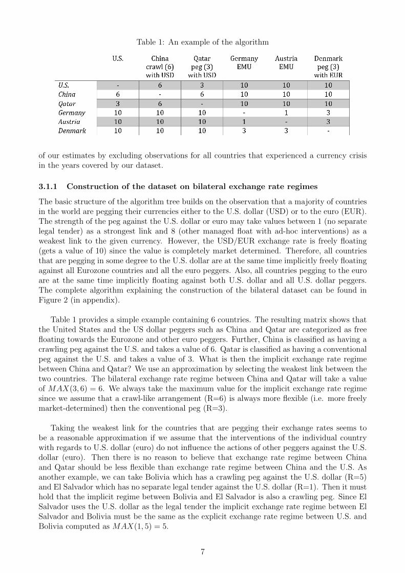
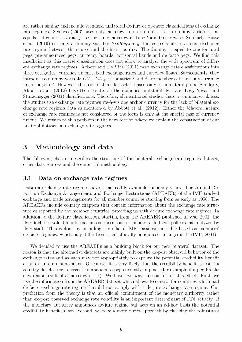
Table 1: An example of the algorithm

of our estimates by excluding observations for all countries that experienced a currency crisisin the years covered by our dataset.

3.1.1 Construction of the dataset on bilateral exchange rate regimes

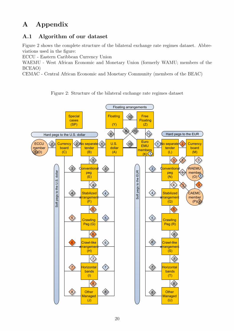
The basic structure of the algorithm tree builds on the observation that a majority of countriesin the world are pegging their currencies either to the U.S. dollar (USD) or to the euro (EUR).The strength of the peg against the U.S. dollar or euro may take values between 1 (no separatelegal tender) as a strongest link and 8 (other managed float with ad-hoc interventions) as aweakest link to the given currency. However, the USD/EUR exchange rate is freely floating(gets a value of 10) since the value is completely market determined. Therefore, all countriesthat are pegging in some degree to the U.S. dollar are at the same time implicitly freely floatingagainst all Eurozone countries and all the euro peggers. Also, all countries pegging to the euroare at the same time implicitly floating against both U.S. dollar and all U.S. dollar peggers.The complete algorithm explaining the construction of the bilateral dataset can be found inFigure 2 (in appendix).

Table 1 provides a simple example containing 6 countries. The resulting matrix shows thatthe United States and the US dollar peggers such as China and Qatar are categorized as freefloating towards the Eurozone and other euro peggers. Further, China is classified as having acrawling peg against the U.S. and takes a value of 6. Qatar is classified as having a conventionalpeg against the U.S. and takes a value of 3. What is then the implicit exchange rate regimebetween China and Qatar? We use an approximation by selecting the weakest link between thetwo countries. The bilateral exchange rate regime between China and Qatar will take a valueof MAX(3, 6) = 6. We always take the maximum value for the implicit exchange rate regimesince we assume that a crawl-like arrangement (R=6) is always more flexible (i.e. more freelymarket-determined) then the conventional peg (R=3).

Taking the weakest link for the countries that are pegging their exchange rates seems tobe a reasonable approximation if we assume that the interventions of the individual countrywith regards to U.S. dollar (euro) do not influence the actions of other peggers against the U.S.dollar (euro). Then there is no reason to believe that exchange rate regime between Chinaand Qatar should be less flexible than exchange rate regime between China and the U.S. Asanother example, we can take Bolivia which has a crawling peg against the U.S. dollar (R=5)and El Salvador which has no separate legal tender against the U.S. dollar (R=1). Then it musthold that the implicit regime between Bolivia and El Salvador is also a crawling peg. Since ElSalvador uses the U.S. dollar as the legal tender the implicit exchange rate regime between ElSalvador and Bolivia must be the same as the explicit exchange rate regime between U.S. andBolivia computed as MAX(1, 5) = 5.

7

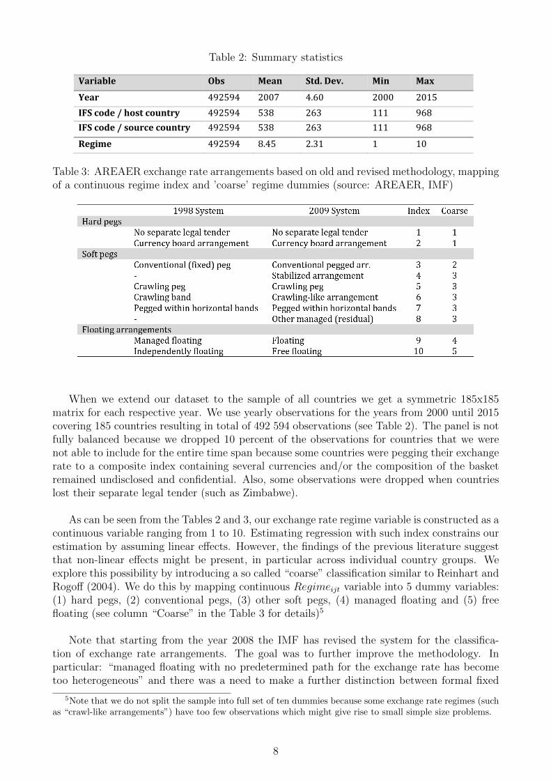
Table 2: Summary statistics

Variable Obs Mean Std. Dev. Min Max

Year 492594 2007 4.60 2000 2015

IFS code / host country 492594 538 263 111 968

IFS code / source country 492594 538 263 111 968

Regime 492594 8.45 2.31 1 10

Table 3: AREAER exchange rate arrangements based on old and revised methodology, mappingof a continuous regime index and ’coarse’ regime dummies (source: AREAER, IMF)

When we extend our dataset to the sample of all countries we get a symmetric 185x185matrix for each respective year. We use yearly observations for the years from 2000 until 2015covering 185 countries resulting in total of 492 594 observations (see Table 2). The panel is notfully balanced because we dropped 10 percent of the observations for countries that we werenot able to include for the entire time span because some countries were pegging their exchangerate to a composite index containing several currencies and/or the composition of the basketremained undisclosed and confidential. Also, some observations were dropped when countrieslost their separate legal tender (such as Zimbabwe).

As can be seen from the Tables 2 and 3, our exchange rate regime variable is constructed as acontinuous variable ranging from 1 to 10. Estimating regression with such index constrains ourestimation by assuming linear effects. However, the findings of the previous literature suggestthat non-linear effects might be present, in particular across individual country groups. Weexplore this possibility by introducing a so called “coarse” classification similar to Reinhart andRogoff (2004). We do this by mapping continuous Regimeijt variable into 5 dummy variables:(1) hard pegs, (2) conventional pegs, (3) other soft pegs, (4) managed floating and (5) freefloating (see column “Coarse” in the Table 3 for details)5

Note that starting from the year 2008 the IMF has revised the system for the classifica-tion of exchange rate arrangements. The goal was to further improve the methodology. Inparticular: “managed floating with no predetermined path for the exchange rate has becometoo heterogeneous” and there was a need to make a further distinction between formal fixed

5Note that we do not split the sample into full set of ten dummies because some exchange rate regimes (suchas “crawl-like arrangements”) have too few observations which might give rise to small simple size problems.

8

Figure 1: Evolution of bilateral exchange rate regimes over time: The number of country-pairsfalling into a certain category (source: own computation)

and crawling pegs and arrangements that are merely peg-like or crawl-like (IMF, 2008). Ourmapping of both the old and the new methodology is reported in the Table 3. The evolutionof the exchange rate regimes over time is shown in the Figure 1. Here we simplified the picturesuch that we categorized the 10 different regimes into 3 groups: Hard pegs (regimes 1 and 2),soft pegs (regimes 3, 4, 5, 6, 7 and 8) and floating arrangements (regimes 9 and 10). It can beseen from the Figure 1 that hard pegs make up only a small share of bilateral exchange rateregimes. This is what we expect to observe given the structure of our dataset which uses aweakest link between the two countries. Also, from a bilateral perspective only relatively smallshare of countries is connected via direct or indirect pegs.

It is to note that the bilateral exchange rate regimes data have been used before for exami-nation of international trade by Klein and Shambaugh (2006). The authors introduced so called“de-facto bilateral exchange rate arrangements” using the dataset of Shambaugh (2004). How-ever, the approach taken by the authors was different from ours: The classification examineswhether a currency stayed within certain pre-defined band against the base currency so it relieson ex-post de-facto observations. The dataset ranges from 1973 to 1999 and it differentiatesonly between direct pegs, indirect pegs and currency unions. We believe that our dataset hasan advantage because it controls for de-facto exchange rate regimes which deviate from theofficial de-jure announcements of monetary authorities. It is s also more granular because itdistinguishes between 10 categories of exchange rate regimes ranging from hard pegs to freefloats.

3.2 Estimation methodology and remaining data sources

We begin our estimation using a gravity-type model across country-pairs and over time withhost country, source country and year fixed effects. Our basic model specification reads asfollows:

9

ln(FDIijt) = α0 + βRegimeijt + γ1JFhostjt + γ2JFsourceit + δ′Wijt+

φ′Xjt + λ′Yit + ϕ′Zij + αi + αj + ξt + εijt(1)

where FDIijt denotes inward direct investment stock positions from country i (source) to coun-try j (host) at time t. Regimeijt denotes a continuous exchange rate regime index taking thevalues from 1 until 10 as described in the Table 2. JFhostjt (JFsourceit) denotes a dummyvariable if the host (source) country has a de-jure exchange rate regime that differs from its defacto exchange rate regime by more than 1 degree. We expect all three coefficients β, γ1 and γ2to be negative and statistically significant. Wijt denotes a set of bilateral time-variant controlvariables, Xjt (Yit) denotes a set of time-variant control variables of the host (source) country,Zij denotes the set of bilateral time-invariant control variables, αi (αj) denotes source (host)country fixed effects and ξt denotes year fixed effects.

Although the estimation using OLS estimates of the gravity model is informative, it hasseveral important drawbacks: First drawback is that observations with zero values are dropped(logarithm of zero is undefined). A common practice in the literature6 is to perform a “replace-ment” approach of the dependent variable such that all non-positive values will be assigned avalue of 1 such that taking the logarithm is possible and the observations are not lost:

FDIadjijt =

{1 if FDIijt ≤ 0

1 + FDIijt if FDIijt > 0

We decided not to follow this approach and drop the non-positive values.7 Another commondrawback of the OLS estimation specified in the equation (1), as highlighted by Santos Silvaand Tenreyro (2006), is that the parameters of log-linearised models estimated by OLS lead tobiased estimates of the true elasticities. The authors argue that this problem can be fixed byusing a Poisson estimator. Shepherd (2013) recommends that the Poisson results should alwaysbe presented for comparative purposes to avoid the problem of heteroskedasticity in the originalOLS. Another benefit of using the Poisson estimator is that it allows us to include observationsfor which the observed FDI were zero, which results in our case in twice as large sample sizecompared to the OLS estimation. We follow the recommendation of Shepherd (2013) and usethe “Poisson Pseudo-Maximum Likelihood Estimator” (PPML) command developed by SantosSilva and Tenreyro (2011b). Our “PPML” model specification reads as follows:

FDIijt = α0 + βRegimeijt + γ1JFhostjt + γ2JFsourceit + δ′Wijt

+φ′Xjt + λ′Yit + ϕ′Zij + αi + αj + ξt + εijt(2)

where the only difference to the equation (1) is that the independent variable (FDI stock) isnow entered in levels. Equations (1) and (2) use a continuous exchange rate regime variable(Regimeijt). Further, we test for the existence of non-linear effects using the dummy-based“coarse” classification as explained in the Table 3. The model specification reads as follows:

FDIijt = α0 +4∑

K=1

βKRegimeK,ijt + γ1JFhostjt + γ2JFsourceit + δ′Wijt

+φ′Xjt + λ′Yit + ϕ′Zij + αi + αj + ξt + εijt

(3)

6See Schiavo (2007) or Busse et al. (2010).7First, we would artificially change the value of 58 percent of our observations, 12 percent of which are

negative. Second, the main argument of Busse et al. (2010) to justify the “replace” approach as an aim to haveas many observations as possible. However, we already have more than 30.000 observations even if we drop thezeros given the bilateral structure of our dataset.

10

where∑4

K=1 βKRegimeK,ijt is a vector of exchange rate regime dummies from 1 (hard pegs) to4 (managed floating). The free floating dummy (5) was excluded such that we are comparingeach of the remaining four dummies against the free floating case. We test the equation (3)using the “PPML” estimator with the independent variable (FDI stock) entered in levels.

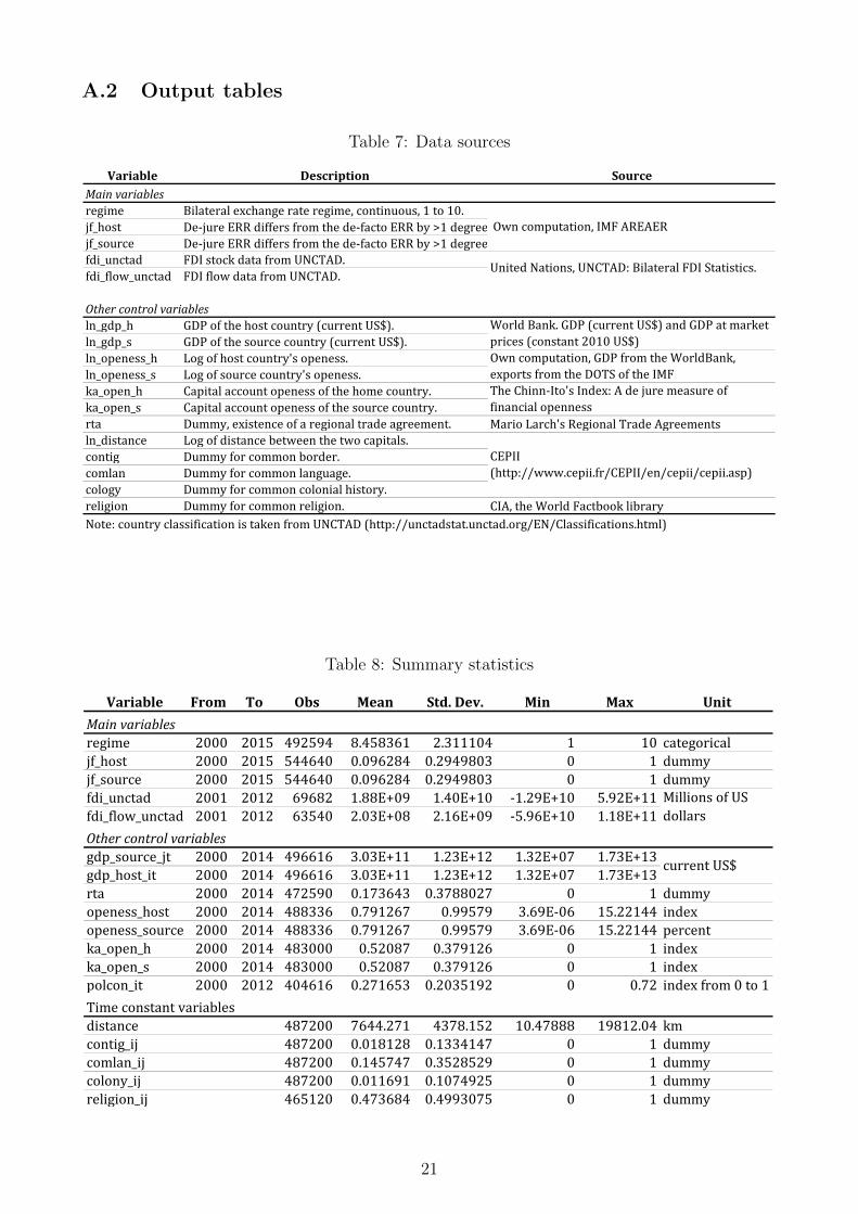
The data sources and summary statistics of the data are listed in the appendix in Tables7 and 8, respectively. The time-variant bilateral control variables include the logs of the hostand source countries’ GDP (ln.gdp.hjt and ln.gdp.sit); trade openness (ln.openness.hjt andln.openness.sit) and capital account openness (ka.open.hjt and ka.open.sit). A dummy for theexistence of regional and trade agreements is denoted by rtaijt. Bilateral time-invariant controlvariables include the distance between two capitals (ln.distanceij) and dummies for commonborder (contigij), common language (comlanij), colonial history (colonyij) and common religion(religionij). We expect the signs of all explanatory variables - with the exception of distance -to be positive.

FDI data available for the years 2001 until 2012 are taken from the UNCTAD. Althoughthe majority of FDI studies uses flow instead of stock data, we decided to use the bilateralUNCTAD stock data as our baseline specification in line with Daude and Fratzscher (2007).The authors preferred to use the stock data due to the fact that the capital stock does notchange strongly over time. We find that the use of the stock data when evaluating the effectsof exchange rate regimes is also preferable because the exchange rate regimes do not frequentlychange over time. Also, less observations have to be dropped since FDI flows frequently takenegative values, which is not the case for FDI stocks. Wacker (2015) argues that in theoryit should not matter whether we use FDI flows or FDI stocks because the former are only ahomogeneous function of the latter. He shows that the correlation in the data between stocksand flows is very high. However, to make sure that the results are consistent, we also compareour results using the flow data. Indeed, we can confirm that the results of our estimation arevery similar notwithstanding whether we use the stocks of flows. We discuss this issue furtherin the section 5.

4 Empirical Results

We report our baseline results of the OLS and PPML estimators from equations (1) and (2).Further, we include estimations for country groups depending on whether the host country isa developing or developed country.

4.1 Baseline estimation using the flexibility index

Table 4 reports the results from the estimation of the equations (1) and (2) with host country,source country and time fixed effects. Columns 1 to 5 report the results for OLS and columns 6to 10 report the results for PPML. Columns 1 and 6 include only the basic specification includ-ing exchange rate regime dummies and log of the GDP of the host and source country. Furtherexplanatory variables are included in the subsequent columns. The distance variable is includedin columns 4 and 9. Full specification in columns 5 and 10 can be seen as our benchmark result.

From Table 4 can be seen that all coefficients of the standard gravity variables have theexpected signs. For example, it can be seen from column 5 that a 1 per cent increase in hostcountry’s GDP is associated with a 65 percent higher FDI stock (exp(0.499)-1). Looking atthe distance coefficient, a 1 percent increase in distance is associated with a decrease in FDIby around 1.65 percent, and this effect is significant at the 1 percent level. This effect is larger

11

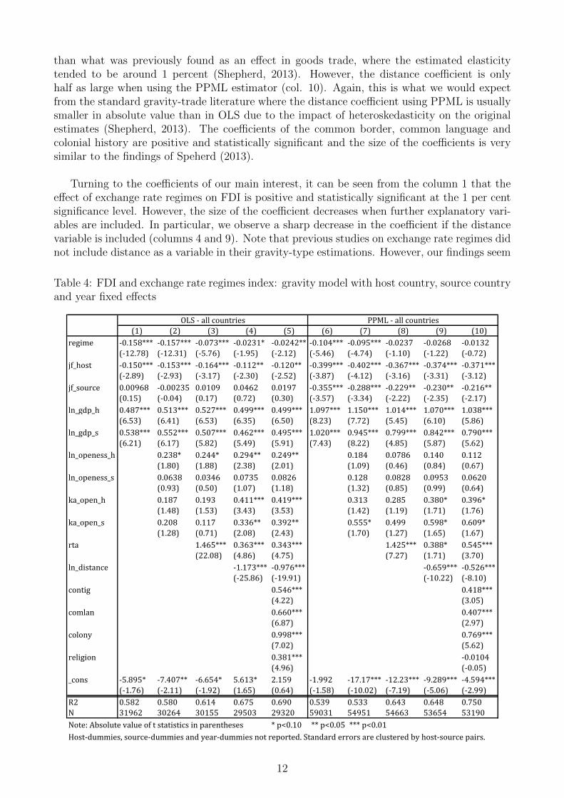
than what was previously found as an effect in goods trade, where the estimated elasticitytended to be around 1 percent (Shepherd, 2013). However, the distance coefficient is onlyhalf as large when using the PPML estimator (col. 10). Again, this is what we would expectfrom the standard gravity-trade literature where the distance coefficient using PPML is usuallysmaller in absolute value than in OLS due to the impact of heteroskedasticity on the originalestimates (Shepherd, 2013). The coefficients of the common border, common language andcolonial history are positive and statistically significant and the size of the coefficients is verysimilar to the findings of Speherd (2013).

Turning to the coefficients of our main interest, it can be seen from the column 1 that theeffect of exchange rate regimes on FDI is positive and statistically significant at the 1 per centsignificance level. However, the size of the coefficient decreases when further explanatory vari-ables are included. In particular, we observe a sharp decrease in the coefficient if the distancevariable is included (columns 4 and 9). Note that previous studies on exchange rate regimes didnot include distance as a variable in their gravity-type estimations. However, our findings seem

Table 4: FDI and exchange rate regimes index: gravity model with host country, source countryand year fixed effects

(1) (2) (3) (4) (5) (6) (7) (8) (9) (10)

regime -0.158*** -0.157*** -0.073*** -0.0231* -0.0242** -0.104*** -0.095*** -0.0237 -0.0268 -0.0132

(-12.78) (-12.31) (-5.76) (-1.95) (-2.12) (-5.46) (-4.74) (-1.10) (-1.22) (-0.72)

jf_host -0.150*** -0.153*** -0.164*** -0.112** -0.120** -0.399*** -0.402*** -0.367*** -0.374*** -0.371***

(-2.89) (-2.93) (-3.17) (-2.30) (-2.52) (-3.87) (-4.12) (-3.16) (-3.31) (-3.12)

jf_source 0.00968 -0.00235 0.0109 0.0462 0.0197 -0.355*** -0.288*** -0.229** -0.230** -0.216**

(0.15) (-0.04) (0.17) (0.72) (0.30) (-3.57) (-3.34) (-2.22) (-2.35) (-2.17)

ln_gdp_h 0.487*** 0.513*** 0.527*** 0.499*** 0.499*** 1.097*** 1.150*** 1.014*** 1.070*** 1.038***

(6.53) (6.41) (6.53) (6.35) (6.50) (8.23) (7.72) (5.45) (6.10) (5.86)

ln_gdp_s 0.538*** 0.552*** 0.507*** 0.462*** 0.495*** 1.020*** 0.945*** 0.799*** 0.842*** 0.790***

(6.21) (6.17) (5.82) (5.49) (5.91) (7.43) (8.22) (4.85) (5.87) (5.62)

ln_openess_h 0.238* 0.244* 0.294** 0.249** 0.184 0.0786 0.140 0.112

(1.80) (1.88) (2.38) (2.01) (1.09) (0.46) (0.84) (0.67)

ln_openess_s 0.0638 0.0346 0.0735 0.0826 0.128 0.0828 0.0953 0.0620

(0.93) (0.50) (1.07) (1.18) (1.32) (0.85) (0.99) (0.64)

ka_open_h 0.187 0.193 0.411*** 0.419*** 0.313 0.285 0.380* 0.396*

(1.48) (1.53) (3.43) (3.53) (1.42) (1.19) (1.71) (1.76)

ka_open_s 0.208 0.117 0.336** 0.392** 0.555* 0.499 0.598* 0.609*

(1.28) (0.71) (2.08) (2.43) (1.70) (1.27) (1.65) (1.67)

rta 1.465*** 0.363*** 0.343*** 1.425*** 0.388* 0.545***

(22.08) (4.86) (4.75) (7.27) (1.71) (3.70)

ln_distance -1.173*** -0.976*** -0.659*** -0.526***

(-25.86) (-19.91) (-10.22) (-8.10)

contig 0.546*** 0.418***

(4.22) (3.05)

comlan 0.660*** 0.407***

(6.87) (2.97)

colony 0.998*** 0.769***

(7.02) (5.62)

religion 0.381*** -0.0104

(4.96) (-0.05)

_cons -5.895* -7.407** -6.654* 5.613* 2.159 -1.992 -17.17*** -12.23*** -9.289*** -4.594***

(-1.76) (-2.11) (-1.92) (1.65) (0.64) (-1.58) (-10.02) (-7.19) (-5.06) (-2.99)

R2 0.582 0.580 0.614 0.675 0.690 0.539 0.533 0.643 0.648 0.750

N 31962 30264 30155 29503 29320 59031 54951 54663 53654 53190

Note: Absolute value of t statistics in parentheses * p<0.10 ** p<0.05 *** p<0.01

Host-dummies, source-dummies and year-dummies not reported. Standard errors are clustered by host-source pairs.

OLS - all countries PPML - all countries

12

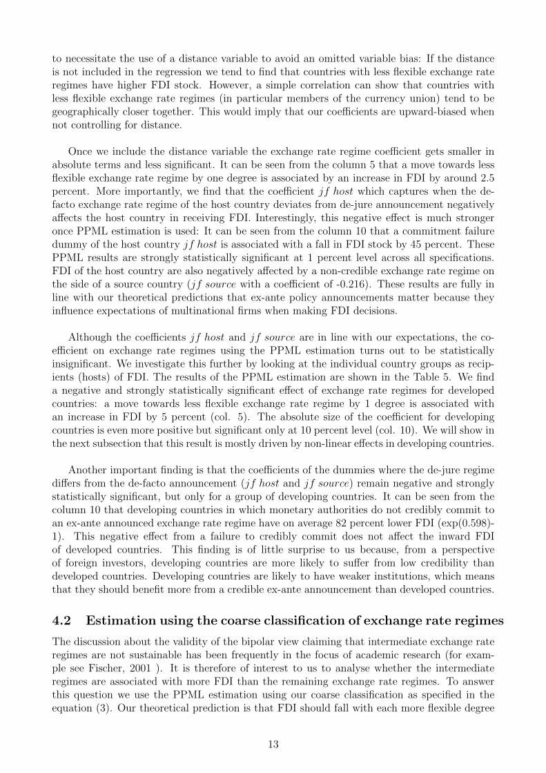
to necessitate the use of a distance variable to avoid an omitted variable bias: If the distanceis not included in the regression we tend to find that countries with less flexible exchange rateregimes have higher FDI stock. However, a simple correlation can show that countries withless flexible exchange rate regimes (in particular members of the currency union) tend to begeographically closer together. This would imply that our coefficients are upward-biased whennot controlling for distance.

Once we include the distance variable the exchange rate regime coefficient gets smaller inabsolute terms and less significant. It can be seen from the column 5 that a move towards lessflexible exchange rate regime by one degree is associated by an increase in FDI by around 2.5percent. More importantly, we find that the coefficient jf host which captures when the de-facto exchange rate regime of the host country deviates from de-jure announcement negativelyaffects the host country in receiving FDI. Interestingly, this negative effect is much strongeronce PPML estimation is used: It can be seen from the column 10 that a commitment failuredummy of the host country jf host is associated with a fall in FDI stock by 45 percent. ThesePPML results are strongly statistically significant at 1 percent level across all specifications.FDI of the host country are also negatively affected by a non-credible exchange rate regime onthe side of a source country (jf source with a coefficient of -0.216). These results are fully inline with our theoretical predictions that ex-ante policy announcements matter because theyinfluence expectations of multinational firms when making FDI decisions.

Although the coefficients jf host and jf source are in line with our expectations, the co-efficient on exchange rate regimes using the PPML estimation turns out to be statisticallyinsignificant. We investigate this further by looking at the individual country groups as recip-ients (hosts) of FDI. The results of the PPML estimation are shown in the Table 5. We finda negative and strongly statistically significant effect of exchange rate regimes for developedcountries: a move towards less flexible exchange rate regime by 1 degree is associated withan increase in FDI by 5 percent (col. 5). The absolute size of the coefficient for developingcountries is even more positive but significant only at 10 percent level (col. 10). We will show inthe next subsection that this result is mostly driven by non-linear effects in developing countries.

Another important finding is that the coefficients of the dummies where the de-jure regimediffers from the de-facto announcement (jf host and jf source) remain negative and stronglystatistically significant, but only for a group of developing countries. It can be seen from thecolumn 10 that developing countries in which monetary authorities do not credibly commit toan ex-ante announced exchange rate regime have on average 82 percent lower FDI (exp(0.598)-1). This negative effect from a failure to credibly commit does not affect the inward FDIof developed countries. This finding is of little surprise to us because, from a perspectiveof foreign investors, developing countries are more likely to suffer from low credibility thandeveloped countries. Developing countries are likely to have weaker institutions, which meansthat they should benefit more from a credible ex-ante announcement than developed countries.

4.2 Estimation using the coarse classification of exchange rate regimes

The discussion about the validity of the bipolar view claiming that intermediate exchange rateregimes are not sustainable has been frequently in the focus of academic research (for exam-ple see Fischer, 2001 ). It is therefore of interest to us to analyse whether the intermediateregimes are associated with more FDI than the remaining exchange rate regimes. To answerthis question we use the PPML estimation using our coarse classification as specified in theequation (3). Our theoretical prediction is that FDI should fall with each more flexible degree

13

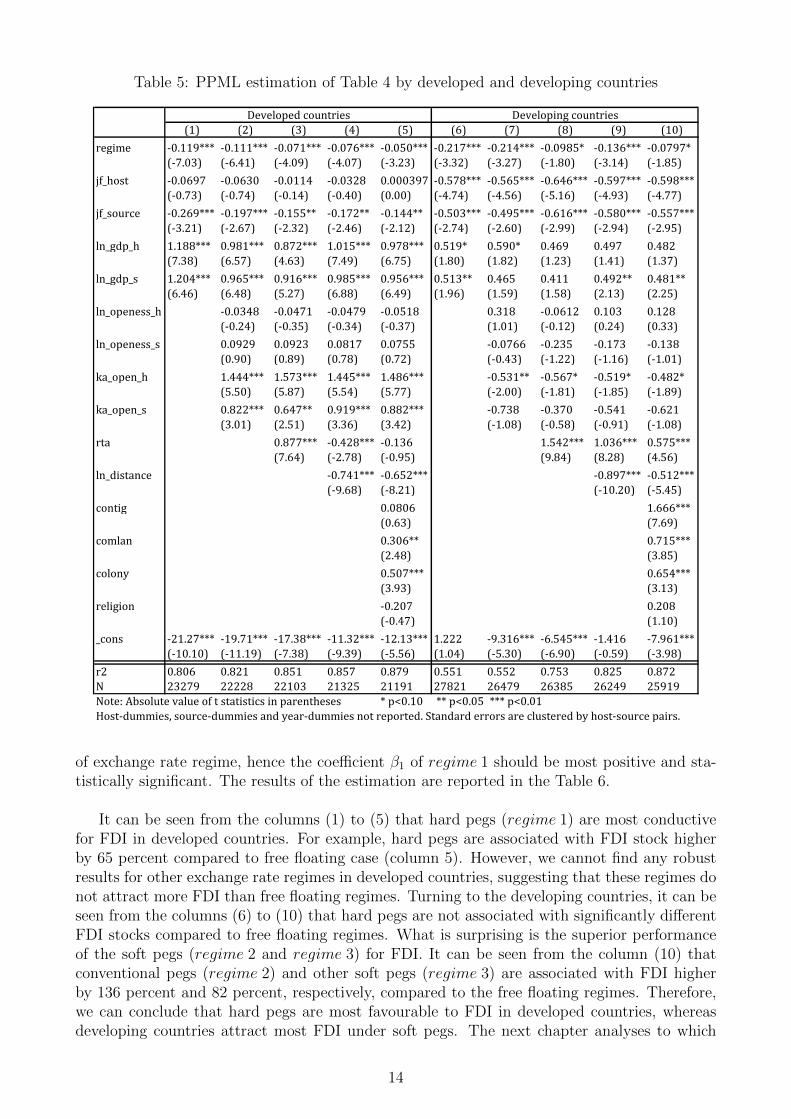
Table 5: PPML estimation of Table 4 by developed and developing countries

(1) (2) (3) (4) (5) (6) (7) (8) (9) (10)

regime -0.119*** -0.111*** -0.071*** -0.076*** -0.050*** -0.217*** -0.214*** -0.0985* -0.136*** -0.0797*

(-7.03) (-6.41) (-4.09) (-4.07) (-3.23) (-3.32) (-3.27) (-1.80) (-3.14) (-1.85)

jf_host -0.0697 -0.0630 -0.0114 -0.0328 0.000397 -0.578*** -0.565*** -0.646*** -0.597*** -0.598***

(-0.73) (-0.74) (-0.14) (-0.40) (0.00) (-4.74) (-4.56) (-5.16) (-4.93) (-4.77)

jf_source -0.269*** -0.197*** -0.155** -0.172** -0.144** -0.503*** -0.495*** -0.616*** -0.580*** -0.557***

(-3.21) (-2.67) (-2.32) (-2.46) (-2.12) (-2.74) (-2.60) (-2.99) (-2.94) (-2.95)

ln_gdp_h 1.188*** 0.981*** 0.872*** 1.015*** 0.978*** 0.519* 0.590* 0.469 0.497 0.482

(7.38) (6.57) (4.63) (7.49) (6.75) (1.80) (1.82) (1.23) (1.41) (1.37)

ln_gdp_s 1.204*** 0.965*** 0.916*** 0.985*** 0.956*** 0.513** 0.465 0.411 0.492** 0.481**

(6.46) (6.48) (5.27) (6.88) (6.49) (1.96) (1.59) (1.58) (2.13) (2.25)

ln_openess_h -0.0348 -0.0471 -0.0479 -0.0518 0.318 -0.0612 0.103 0.128

(-0.24) (-0.35) (-0.34) (-0.37) (1.01) (-0.12) (0.24) (0.33)

ln_openess_s 0.0929 0.0923 0.0817 0.0755 -0.0766 -0.235 -0.173 -0.138

(0.90) (0.89) (0.78) (0.72) (-0.43) (-1.22) (-1.16) (-1.01)

ka_open_h 1.444*** 1.573*** 1.445*** 1.486*** -0.531** -0.567* -0.519* -0.482*

(5.50) (5.87) (5.54) (5.77) (-2.00) (-1.81) (-1.85) (-1.89)

ka_open_s 0.822*** 0.647** 0.919*** 0.882*** -0.738 -0.370 -0.541 -0.621

(3.01) (2.51) (3.36) (3.42) (-1.08) (-0.58) (-0.91) (-1.08)

rta 0.877*** -0.428*** -0.136 1.542*** 1.036*** 0.575***

(7.64) (-2.78) (-0.95) (9.84) (8.28) (4.56)

ln_distance -0.741*** -0.652*** -0.897*** -0.512***

(-9.68) (-8.21) (-10.20) (-5.45)

contig 0.0806 1.666***

(0.63) (7.69)

comlan 0.306** 0.715***

(2.48) (3.85)

colony 0.507*** 0.654***

(3.93) (3.13)

religion -0.207 0.208

(-0.47) (1.10)

_cons -21.27*** -19.71*** -17.38*** -11.32*** -12.13*** 1.222 -9.316*** -6.545*** -1.416 -7.961***

(-10.10) (-11.19) (-7.38) (-9.39) (-5.56) (1.04) (-5.30) (-6.90) (-0.59) (-3.98)

r2 0.806 0.821 0.851 0.857 0.879 0.551 0.552 0.753 0.825 0.872

N 23279 22228 22103 21325 21191 27821 26479 26385 26249 25919

Note: Absolute value of t statistics in parentheses * p<0.10 ** p<0.05 *** p<0.01

Host-dummies, source-dummies and year-dummies not reported. Standard errors are clustered by host-source pairs.

Developed countries Developing countries

of exchange rate regime, hence the coefficient β1 of regime 1 should be most positive and sta-tistically significant. The results of the estimation are reported in the Table 6.

It can be seen from the columns (1) to (5) that hard pegs (regime 1) are most conductivefor FDI in developed countries. For example, hard pegs are associated with FDI stock higherby 65 percent compared to free floating case (column 5). However, we cannot find any robustresults for other exchange rate regimes in developed countries, suggesting that these regimes donot attract more FDI than free floating regimes. Turning to the developing countries, it can beseen from the columns (6) to (10) that hard pegs are not associated with significantly differentFDI stocks compared to free floating regimes. What is surprising is the superior performanceof the soft pegs (regime 2 and regime 3) for FDI. It can be seen from the column (10) thatconventional pegs (regime 2) and other soft pegs (regime 3) are associated with FDI higherby 136 percent and 82 percent, respectively, compared to the free floating regimes. Therefore,we can conclude that hard pegs are most favourable to FDI in developed countries, whereasdeveloping countries attract most FDI under soft pegs. The next chapter analyses to which

14

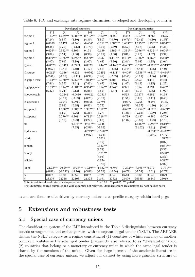
Table 6: FDI and exchange rate regimes dummies: developed and developing countries

(1) (2) (3) (4) (5) (6) (7) (8) (9) (10)

regime 1 1.116*** 1.039*** 0.680*** 0.736*** 0.502*** -0.358 -0.362 -0.869** -0.263 -0.676

(7.24) (6.59) (4.30) (4.30) (3.50) (-0.70) (-0.71) (-2.41) (-0.80) (-1.53)

regime 2 0.0809 0.0477 -0.268 -0.404* -0.611*** 1.686*** 1.685*** 1.095*** 1.130*** 0.860***

(0.35) (0.20) (-1.13) (-1.79) (-3.10) (5.59) (5.52) (4.17) (5.06) (4.35)

regime 3 0.626*** 0.582*** 0.308* 0.171 -0.139 1.382*** 1.381*** 0.796*** 0.832*** 0.604***

(3.82) (3.51) (1.80) (0.98) (-0.99) (3.80) (3.81) (3.22) (4.02) (3.37)

regime 4 0.389*** 0.375*** 0.292** 0.239** 0.156 0.415** 0.434** 0.326** 0.269* 0.258**

(3.07) (2.94) (2.39) (2.07) (1.63) (2.50) (2.41) (2.03) (1.85) (2.01)

jf_host -0.0523 -0.0427 0.0399 0.0979 0.244*** -0.463*** -0.439*** -0.550*** -0.523*** -0.513***

(-0.52) (-0.46) (0.48) (1.17) (2.58) (-3.66) (-3.44) (-4.44) (-4.06) (-4.01)

jf_source -0.262** -0.186* -0.122 -0.0762 0.0452 -0.411** -0.408** -0.538*** -0.510*** -0.484***

(-2.41) (-1.90) (-1.41) (-0.90) (0.49) (-2.55) (-2.45) (-3.11) (-3.06) (-2.83)

ln_gdp_h_resc 1.182*** 0.978*** 0.868*** 1.012*** 0.972*** 0.385 0.521 0.453 0.473 0.458

(7.41) (6.55) (4.61) (7.43) (6.67) (1.30) (1.47) (1.18) (1.25) (1.25)

ln_gdp_s_resc 1.159*** 0.914*** 0.881*** 0.964*** 0.954*** 0.367* 0.321 0.354 0.391 0.427*

(6.22) (6.21) (5.12) (6.86) (6.52) (1.67) (1.38) (1.35) (1.56) (1.92)

ln_openess_h -0.0246 -0.0450 -0.0421 -0.0519 0.523 0.0279 0.188 0.198

(-0.17) (-0.33) (-0.29) (-0.37) (1.51) (0.06) (0.41) (0.49)

ln_openess_s 0.0947 0.0911 0.0866 0.0794 -0.0877 -0.255 -0.193 -0.155

(0.92) (0.88) (0.83) (0.75) (-0.51) (-1.27) (-1.20) (-1.14)

ka_open_h 1.500*** 1.586*** 1.392*** 1.352*** -0.607* -0.754** -0.628* -0.609**

(5.69) (5.96) (5.38) (5.27) (-1.88) (-2.03) (-1.89) (-2.04)

ka_open_s 0.770*** 0.561** 0.782*** 0.718*** -0.759 -0.487 -0.580 -0.709

(3.10) (2.23) (3.27) (3.02) (-1.02) (-0.68) (-0.93) (-1.15)

rta 0.875*** -0.437*** -0.145 1.526*** 1.096*** 0.610***

(7.65) (-2.86) (-1.02) (11.02) (8.81) (5.02)

ln_distance -0.749*** -0.668*** -0.831*** -0.442***

(-9.82) (-8.36) (-10.49) (-4.72)

contig 0.0624 1.597***

(0.49) (8.07)

comlan 0.323*** 0.831***

(2.74) (5.35)

colony 0.521*** 0.508**

(4.05) (2.51)

religion -0.254 0.397**

(-0.58) (2.02)

_cons -21.23*** -20.59*** -19.33*** -10.19*** -14.32*** -0.794 -7.272*** -7.695*** 0.979 -3.781***

(-8.82) (-12.12) (-9.76) (-5.80) (-7.78) (-0.54) (-6.71) (-7.54) (0.61) (-2.77)

r2 0.807 0.822 0.852 0.857 0.879 0.640 0.640 0.802 0.843 0.879

N 23279 22228 22103 21325 21191 27821 26479 26385 26249 25919

Note: Absolute value of t statistics in parentheses * p<0.10 ** p<0.05 *** p<0.01

Host-dummies, source-dummies and year-dummies not reported. Standard errors are clustered by host-source pairs.

Developed countries Developing countries

extent are these results driven by currency unions as a specific category within hard pegs.

5 Extensions and robustness tests

5.1 Special case of currency unions

The classification system of the IMF introduced in the Table 3 distinguishes between currencyboards arrangements and exchange rates with no separate legal tender (NSLT). The AREAERdefines the NSLT category as a regime consisting of (1) countries of which currency of anothercountry circulates as the sole legal tender (frequently also referred to as “dollarization”) and(2) countries that belong to a monetary or currency union in which the same legal tender isshared by the members of the union. Given the large interest of the academic literature inthe special case of currency unions, we adjust our dataset by using more granular structure of

15

the data with the special focus on currency unions. We do this by splitting the NSLT regimecategory (regime 1) into the currency union members (cu.nslt.dum) and “dollarized” coun-tries8 (not.cu.nslt.dum) subcategories. Also, we separately include the currency board dummy(cb.dummy) which was previously part of the hard pegs (regime 1).

The results of the PPML estimation are shown in the Table 9 (in Appendix). We can seethat the positive coefficient of regime 1 from the previous Table is driven mostly by the NSLTcategories as the coefficient for the currency boards turns out to be statistically insignificant.Currency unions seem to attract most FDI flows in developed countries. Developed countrieswith no separate legal tender which are not members of the currency union (i.e. “dollarized‘”countries) seem to attract more FDI as well, albeit the coefficient is significant only at the 10percent level (0.688 in col. 5). What regards the developing countries, it can be seen from thecolumn (10) that being a “dollarized” country is associated with FDI stock which is almost 300percent higher (EXP(1.359)-1) compared to free floating regimes. This effect is even strongerthan the coefficients of regimes 2 and 3, which is exactly what we expect from the theory:the more a country departs from a credible peg the lower the FDI that we should observe.However, the coefficients for both currency unions and currency boards of developing countriesremain mostly statistically insignificant and the coefficients are overall quite noisy across thespecifications, which is likely the reason why the coefficient of regime 1 was insignificant in theprevious Table 6.

5.1.1 Accounting for third-country effects of countries belonging to a currencyunion

The property of the dataset built on a bilateral basis is that only members that are insideof a currency union will be captured in the data as belonging to the currency union. Thus,our dummy variable captures whether the currency union results in larger FDI stock betweencurrency union members. However, Schiavo et al.(2007), looking at the special case of the Eu-ropean Monetary Union (EMU), found that the EMU has resulted in larger FDI flows not onlybetween EMU members but also with the rest of the world. We test this finding by creatinga new currency union dummy (cu.dum.unilateral) that equals to one if a host country is amember of currency union in a year t.

We report the results of this extended test using the PPML estimator in the Table 10 (inAppendix). It can be seen that the standard bilateral currency union dummy cu.nslt.dumremains strongly statistically significant. However, the coefficient cu.dum.unilateral is statis-tically insignificant, implying that the pure fact that a country is a member of the currencyunion does not increase FDI. Instead, both sending and recipient countries must be in the samecurrency union to experience an increase in FDI. Therefore, we cannot cannot confirm thefinding of Schiavo that currency union members receive higher FDI from the rest of the world.We find that currency unions are associated with higher FDI inflows from other members ofthe currency area without having any significant effect on the FDI inflows from the countriesfrom the outside of the currency unions.

5.2 Other robustness tests

We noted in the introduction of our paper that the benefit of a credible announcement holdsonly as long as the exchange rate regime in place is credible and does not change. We controlfor this potential endogeneity problem in the data by using dummies for countries that have

8The term “dollarization” does not imply that the currency in circulation has to be the U.S. dollar.

16

de-facto exchange rate regimes which differ from the de-jure announcements. In addition, weaim to control for this more directly by controlling for the occurrences of currency crises. Wedo this by excluding observations for all countries in our sample that were in a currency crisisin any period of time. The results are reported in the Table 11. It can be seen that the resultsare fully in line with our previous findings.

Further robustness tests include the use of FDI flows instead of stocks. One of the reasonswhy we decided to use FDI stock data instead of flow data was that FDI stock data consistsof 47 per cent of observations which are zero and only 2 per cent of observations which arenegative. The FDI flow data consist of 46 per cent of observations which are zero and 12percent of the observations which are negative. If we use the PPML estimator and drop thenegative values the estimation with FDI stocks will lose only 2 percent of the observations,compared to 12 per cent in the case of the estimation with FDI flows. We show the resultsusing the FDI flows specification in the Table 12. We can see that the results are surprisinglysimilar to the FDI stock estimation. Therefore, we are confident that the results are robustto both stock and flow specifications. In addition, we perform further robustness checks whichincluded dropping all countries with population below 1 million, dropping small island statesand using different classification of tax havens. The results for these tests are available uponrequest.

6 Summary and conclusion

By using our newly developed dataset on bilateral exchange rate regimes, we can confirm thefindings of the previous literature that exchange rate regimes are an important determinant ofcross-border investment. We argue that the key channel at work through which exchange rateregimes affect FDI is their ex-ante character based on a policy announcement. This announce-ment is important for foreign investors in forming expectations about the future developmentof the exchange rate. For this channel to work it is crucial for such announcement to becredible. We control for the credibility of the announcement by collecting data on countrieswhere de-facto exchange rate regimes deviate from their ex-ante announced de-jure exchangerate regimes. We find that this credibility effect is particularly strong for developing coun-tries which is in line with our expectations because these countries are likely to have weakerinstitutions than developed countries, thus benefiting more from a credible announcement effect.

Our results further suggest that it is crucial to include a distance variable in the FDI esti-mation to avoid an omitted variable bias problem because countries with less flexible exchangerate regimes, in particular members of the currency union, tend to be geographically closertogether. This would imply that the coefficients are upward-biased when not controlling for thedistance. The results from regression using the individual regimes show that while currencyunions are most favourable to FDI in developed countries, developing countries attract mostFDI under soft pegs.

17

References

[1] A. Abbott, D. O. Cushman, and G. De Vita. Exchange rate regimes and foreign directinvestment flows to developing countries. Review of International Economics, pages 95–107, 2012.

[2] A. Abbott and G. De Vita. Evidence on the impact of exchange rate regimes on bilateralfdi flows. Journal of Economic Studies, 38(3):253–274, 2011.

[3] J. Aizenman. Exchange rate flexibility, volatility and foreign direct investment. IMF StaffPapers, 39:890–922, 1992.

[4] M. Busse, C. Hefeker, and S. Nelgen. Foreign direct investment and exchange rate regimes.MAGKS Papers on Economics, 15-2010, 2010.

[5] Ch. Daude and M. Fratzscher. The pecking order of cross-border investment. Journal ofInternational Economics, 74:94–119, 2008.

[6] A. Faeth. Determinants of foreign direct investment - a tale of nine theoretical models.Journal of Economic Surveys, 23:165–196, 2009.

[7] Stanley Fischer. Exchange Rate Regimes: Is the Bipolar View Correct? Journal ofEconomic Perspectives, 15(2):3–24, Spring 2001.

[8] P. Harms. How does the exchange rate regime affect fdi? a note. Unpublished note,Johannes Gutenberg University Mainz, March 2017.

[9] International Monetary Fund. Annual report on exchange arrangements and exchange re-strictions. http://www.elibrary-areaer.imf.org/Pages/YearlyReports.aspx, 2000-2015.

[10] M. W. Klein and J. C. Shambaugh. Fixed exchange rates and trade. NBER WorkingPaper, 10696, 2004.

[11] M. W. Klein and J. C. Shambaugh. Fixed exchange rates and trade. Journal of Interna-tional Economics, 70:359–383, 2006.

[12] E. Levy-Yeyati and F. Sturzenegger. To float or to fix: Evidence on the impact of exchangerate regimes on growth. American Economic Review, 93:1173–1193, 2003.

[13] C. Reinhart and K. S. Rogoff. The modern history of exchange rate arrangements: areinterpretation. Quarterly Journal of Economics, 119:1–48, 2004.

[14] K. N. Russ. The endogeneity of the exchange rate as a determinant of fdi: A model ofentry and multinational firms. Journal of International Economics, 71(2):344–372, 2007.

[15] K. N. Russ. Exchange rate volatility and first-time entry by multinational firms. Reviewof World Economics, 148(2):269–295, 2012.

[16] J. M. C. Santos Silva and S. Tenreyro. The log of gravity. The Review of Economics andStatistics, 88(4):641–658, 2006.

[17] J. M. C. Santos Silva and S. Tenreyro. Currency unions in prospect and retrospect. AnnualReview of Economics, 2:51–74, 2010.

18

[18] J. M. C. Santos Silva and S. Tenreyro. Poisson: Some convergence issues. Stata Journal,11(2):207–212, 2011b.

[19] S. Schiavo. Common currencies and fdi flows. Oxford Economic Papers, 59(3):536–560,2007.

[20] B. Shepherd. The grativy model of international trade: A user guide. http://www.

unescap.org/sites/default/files/tipub2645.pdf, 2013.

[21] The Teleraph. Jaguar land rover revving up production with new factory in slo-vakia. http://www.telegraph.co.uk/finance/newsbysector/industry/12045191/

Jaguar-Land-Rover-revving-up-production-with-new-factory-in-Slovakia.html,11 Dec 2015.

[22] K. M. Wacker. When should we use foreign direct investment data to measure the activitiesof multinational corporations? theory and evidence. Review of International Economics,24(5):980–999, 2016.

19

A Appendix

A.1 Algorithm of our dataset

Figure 2 shows the complete structure of the bilateral exchange rate regimes dataset. Abbre-viations used in the figure:ECCU - Eastern Caribbean Currency UnionWAEMU - West African Economic and Monetary Union (formerly WAMU; members of theBCEAO)CEMAC - Central African Economic and Monetary Community (members of the BEAC)

Figure 2: Structure of the bilateral exchange rate regimes dataset

20

A.2 Output tables

Table 7: Data sources

Variable Description SourceMain variablesregime Bilateral exchange rate regime, continuous, 1 to 10.jf_host De-jure ERR differs from the de-facto ERR by >1 degree jf_source De-jure ERR differs from the de-facto ERR by >1 degree fdi_unctad FDI stock data from UNCTAD.fdi_flow_unctad FDI flow data from UNCTAD.

Other control variablesln_gdp_h GDP of the host country (current US$).ln_gdp_s GDP of the source country (current US$).ln_openess_h Log of host country's openess.ln_openess_s Log of source country's openess.ka_open_h Capital account openess of the home country. ka_open_s Capital account openess of the source country. rta Dummy, existence of a regional trade agreement. Mario Larch's Regional Trade Agreements ln_distance Log of distance between the two capitals. contig Dummy for common border. comlan Dummy for common language. cology Dummy for common colonial history. religion Dummy for common religion. CIA, the World Factbook libraryNote: country classification is taken from UNCTAD (http://unctadstat.unctad.org/EN/Classifications.html)

The Chinn-Ito's Index: A de jure measure of financial openness

Own computation, GDP from the WorldBank, exports from the DOTS of the IMF

World Bank. GDP (current US$) and GDP at market prices (constant 2010 US$)

CEPII (http://www.cepii.fr/CEPII/en/cepii/cepii.asp)

Own computation, IMF AREAER

United Nations, UNCTAD: Bilateral FDI Statistics.

Table 8: Summary statistics

Variable From To Obs Mean Std. Dev. Min Max UnitMain variablesregime 2000 2015 492594 8.458361 2.311104 1 10 categoricaljf_host 2000 2015 544640 0.096284 0.2949803 0 1 dummyjf_source 2000 2015 544640 0.096284 0.2949803 0 1 dummyfdi_unctad 2001 2012 69682 1.88E+09 1.40E+10 -1.29E+10 5.92E+11fdi_flow_unctad 2001 2012 63540 2.03E+08 2.16E+09 -5.96E+10 1.18E+11Other control variablesgdp_source_jt 2000 2014 496616 3.03E+11 1.23E+12 1.32E+07 1.73E+13gdp_host_it 2000 2014 496616 3.03E+11 1.23E+12 1.32E+07 1.73E+13rta 2000 2014 472590 0.173643 0.3788027 0 1 dummyopeness_host 2000 2014 488336 0.791267 0.99579 3.69E-06 15.22144 indexopeness_source 2000 2014 488336 0.791267 0.99579 3.69E-06 15.22144 percentka_open_h 2000 2014 483000 0.52087 0.379126 0 1 indexka_open_s 2000 2014 483000 0.52087 0.379126 0 1 indexpolcon_it 2000 2012 404616 0.271653 0.2035192 0 0.72 index from 0 to 1Time constant variablesdistance 487200 7644.271 4378.152 10.47888 19812.04 kmcontig_ij 487200 0.018128 0.1334147 0 1 dummycomlan_ij 487200 0.145747 0.3528529 0 1 dummycolony_ij 487200 0.011691 0.1074925 0 1 dummyreligion_ij 465120 0.473684 0.4993075 0 1 dummy

Millions of US dollars

current US$

21

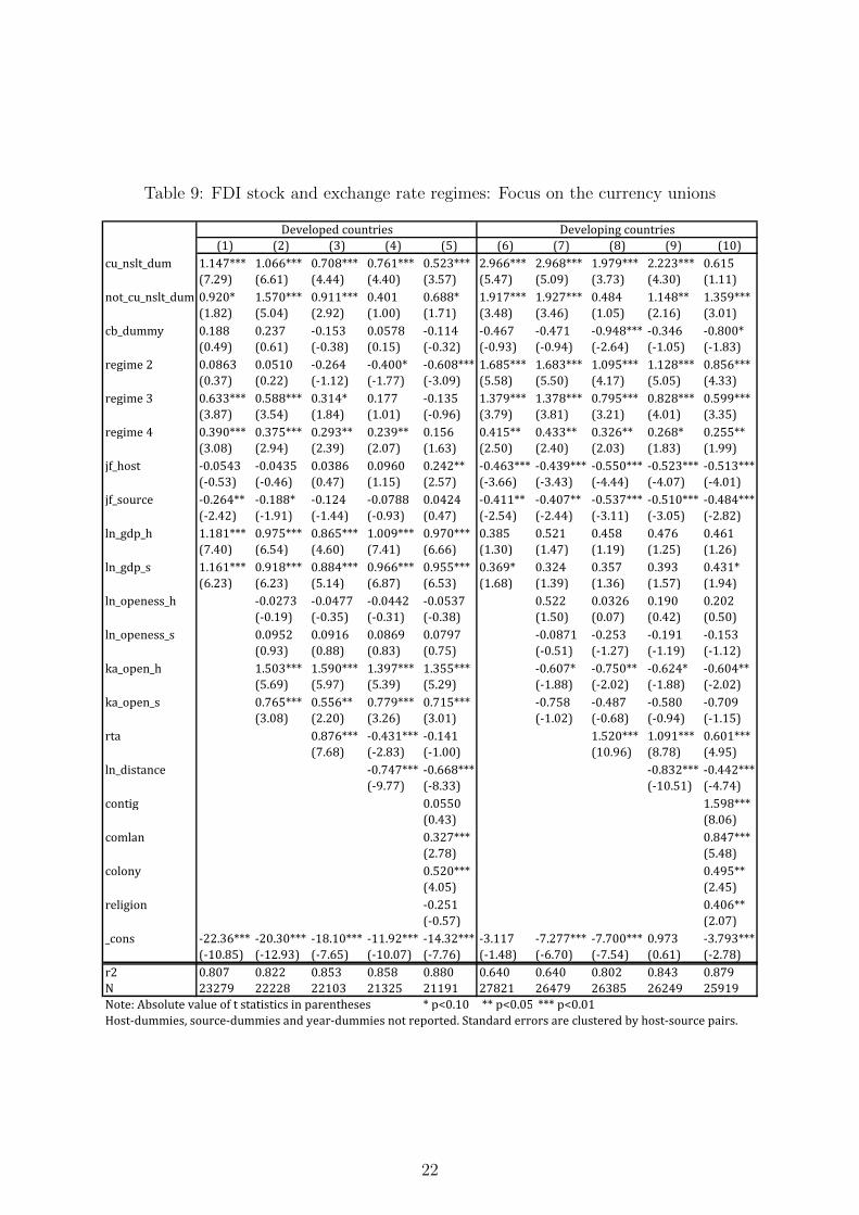
Table 9: FDI stock and exchange rate regimes: Focus on the currency unions

(1) (2) (3) (4) (5) (6) (7) (8) (9) (10)

cu_nslt_dum 1.147*** 1.066*** 0.708*** 0.761*** 0.523*** 2.966*** 2.968*** 1.979*** 2.223*** 0.615

(7.29) (6.61) (4.44) (4.40) (3.57) (5.47) (5.09) (3.73) (4.30) (1.11)

not_cu_nslt_dum 0.920* 1.570*** 0.911*** 0.401 0.688* 1.917*** 1.927*** 0.484 1.148** 1.359***

(1.82) (5.04) (2.92) (1.00) (1.71) (3.48) (3.46) (1.05) (2.16) (3.01)

cb_dummy 0.188 0.237 -0.153 0.0578 -0.114 -0.467 -0.471 -0.948*** -0.346 -0.800*

(0.49) (0.61) (-0.38) (0.15) (-0.32) (-0.93) (-0.94) (-2.64) (-1.05) (-1.83)

regime 2 0.0863 0.0510 -0.264 -0.400* -0.608*** 1.685*** 1.683*** 1.095*** 1.128*** 0.856***

(0.37) (0.22) (-1.12) (-1.77) (-3.09) (5.58) (5.50) (4.17) (5.05) (4.33)

regime 3 0.633*** 0.588*** 0.314* 0.177 -0.135 1.379*** 1.378*** 0.795*** 0.828*** 0.599***

(3.87) (3.54) (1.84) (1.01) (-0.96) (3.79) (3.81) (3.21) (4.01) (3.35)

regime 4 0.390*** 0.375*** 0.293** 0.239** 0.156 0.415** 0.433** 0.326** 0.268* 0.255**

(3.08) (2.94) (2.39) (2.07) (1.63) (2.50) (2.40) (2.03) (1.83) (1.99)

jf_host -0.0543 -0.0435 0.0386 0.0960 0.242** -0.463*** -0.439*** -0.550*** -0.523*** -0.513***

(-0.53) (-0.46) (0.47) (1.15) (2.57) (-3.66) (-3.43) (-4.44) (-4.07) (-4.01)

jf_source -0.264** -0.188* -0.124 -0.0788 0.0424 -0.411** -0.407** -0.537*** -0.510*** -0.484***

(-2.42) (-1.91) (-1.44) (-0.93) (0.47) (-2.54) (-2.44) (-3.11) (-3.05) (-2.82)

ln_gdp_h 1.181*** 0.975*** 0.865*** 1.009*** 0.970*** 0.385 0.521 0.458 0.476 0.461

(7.40) (6.54) (4.60) (7.41) (6.66) (1.30) (1.47) (1.19) (1.25) (1.26)

ln_gdp_s 1.161*** 0.918*** 0.884*** 0.966*** 0.955*** 0.369* 0.324 0.357 0.393 0.431*

(6.23) (6.23) (5.14) (6.87) (6.53) (1.68) (1.39) (1.36) (1.57) (1.94)

ln_openess_h -0.0273 -0.0477 -0.0442 -0.0537 0.522 0.0326 0.190 0.202

(-0.19) (-0.35) (-0.31) (-0.38) (1.50) (0.07) (0.42) (0.50)

ln_openess_s 0.0952 0.0916 0.0869 0.0797 -0.0871 -0.253 -0.191 -0.153

(0.93) (0.88) (0.83) (0.75) (-0.51) (-1.27) (-1.19) (-1.12)

ka_open_h 1.503*** 1.590*** 1.397*** 1.355*** -0.607* -0.750** -0.624* -0.604**

(5.69) (5.97) (5.39) (5.29) (-1.88) (-2.02) (-1.88) (-2.02)

ka_open_s 0.765*** 0.556** 0.779*** 0.715*** -0.758 -0.487 -0.580 -0.709

(3.08) (2.20) (3.26) (3.01) (-1.02) (-0.68) (-0.94) (-1.15)

rta 0.876*** -0.431*** -0.141 1.520*** 1.091*** 0.601***

(7.68) (-2.83) (-1.00) (10.96) (8.78) (4.95)

ln_distance -0.747*** -0.668*** -0.832*** -0.442***

(-9.77) (-8.33) (-10.51) (-4.74)

contig 0.0550 1.598***

(0.43) (8.06)

comlan 0.327*** 0.847***

(2.78) (5.48)

colony 0.520*** 0.495**

(4.05) (2.45)

religion -0.251 0.406**

(-0.57) (2.07)

_cons -22.36*** -20.30*** -18.10*** -11.92*** -14.32*** -3.117 -7.277*** -7.700*** 0.973 -3.793***

(-10.85) (-12.93) (-7.65) (-10.07) (-7.76) (-1.48) (-6.70) (-7.54) (0.61) (-2.78)

r2 0.807 0.822 0.853 0.858 0.880 0.640 0.640 0.802 0.843 0.879

N 23279 22228 22103 21325 21191 27821 26479 26385 26249 25919

Note: Absolute value of t statistics in parentheses * p<0.10 ** p<0.05 *** p<0.01

Host-dummies, source-dummies and year-dummies not reported. Standard errors are clustered by host-source pairs.

Developed countries Developing countries

22

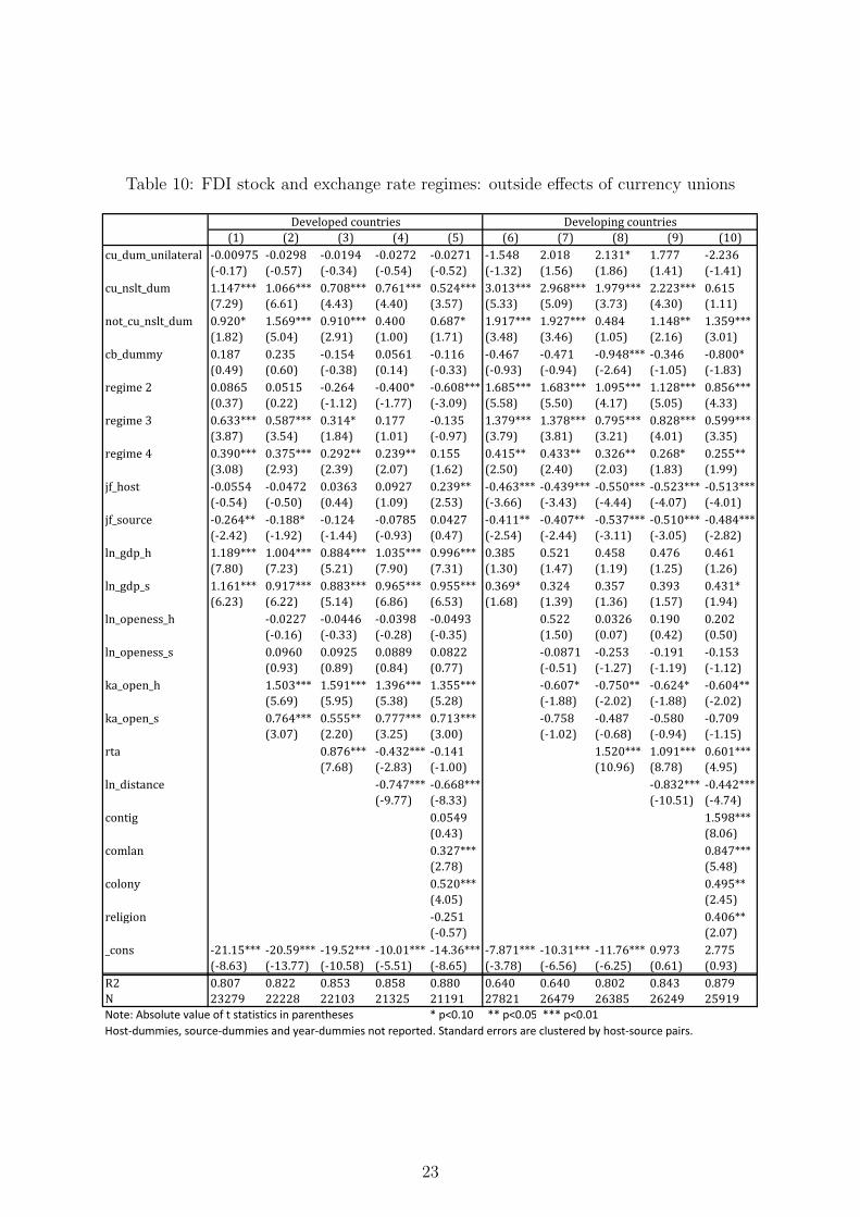
Table 10: FDI stock and exchange rate regimes: outside effects of currency unions

(1) (2) (3) (4) (5) (6) (7) (8) (9) (10)cu_dum_unilateral -0.00975 -0.0298 -0.0194 -0.0272 -0.0271 -1.548 2.018 2.131* 1.777 -2.236

(-0.17) (-0.57) (-0.34) (-0.54) (-0.52) (-1.32) (1.56) (1.86) (1.41) (-1.41)cu_nslt_dum 1.147*** 1.066*** 0.708*** 0.761*** 0.524*** 3.013*** 2.968*** 1.979*** 2.223*** 0.615

(7.29) (6.61) (4.43) (4.40) (3.57) (5.33) (5.09) (3.73) (4.30) (1.11)not_cu_nslt_dum 0.920* 1.569*** 0.910*** 0.400 0.687* 1.917*** 1.927*** 0.484 1.148** 1.359***

(1.82) (5.04) (2.91) (1.00) (1.71) (3.48) (3.46) (1.05) (2.16) (3.01)cb_dummy 0.187 0.235 -0.154 0.0561 -0.116 -0.467 -0.471 -0.948*** -0.346 -0.800*

(0.49) (0.60) (-0.38) (0.14) (-0.33) (-0.93) (-0.94) (-2.64) (-1.05) (-1.83)regime 2 0.0865 0.0515 -0.264 -0.400* -0.608*** 1.685*** 1.683*** 1.095*** 1.128*** 0.856***

(0.37) (0.22) (-1.12) (-1.77) (-3.09) (5.58) (5.50) (4.17) (5.05) (4.33)regime 3 0.633*** 0.587*** 0.314* 0.177 -0.135 1.379*** 1.378*** 0.795*** 0.828*** 0.599***

(3.87) (3.54) (1.84) (1.01) (-0.97) (3.79) (3.81) (3.21) (4.01) (3.35)regime 4 0.390*** 0.375*** 0.292** 0.239** 0.155 0.415** 0.433** 0.326** 0.268* 0.255**

(3.08) (2.93) (2.39) (2.07) (1.62) (2.50) (2.40) (2.03) (1.83) (1.99)jf_host -0.0554 -0.0472 0.0363 0.0927 0.239** -0.463*** -0.439*** -0.550*** -0.523*** -0.513***

(-0.54) (-0.50) (0.44) (1.09) (2.53) (-3.66) (-3.43) (-4.44) (-4.07) (-4.01)jf_source -0.264** -0.188* -0.124 -0.0785 0.0427 -0.411** -0.407** -0.537*** -0.510*** -0.484***

(-2.42) (-1.92) (-1.44) (-0.93) (0.47) (-2.54) (-2.44) (-3.11) (-3.05) (-2.82)ln_gdp_h 1.189*** 1.004*** 0.884*** 1.035*** 0.996*** 0.385 0.521 0.458 0.476 0.461

(7.80) (7.23) (5.21) (7.90) (7.31) (1.30) (1.47) (1.19) (1.25) (1.26)ln_gdp_s 1.161*** 0.917*** 0.883*** 0.965*** 0.955*** 0.369* 0.324 0.357 0.393 0.431*

(6.23) (6.22) (5.14) (6.86) (6.53) (1.68) (1.39) (1.36) (1.57) (1.94)ln_openess_h -0.0227 -0.0446 -0.0398 -0.0493 0.522 0.0326 0.190 0.202

(-0.16) (-0.33) (-0.28) (-0.35) (1.50) (0.07) (0.42) (0.50)ln_openess_s 0.0960 0.0925 0.0889 0.0822 -0.0871 -0.253 -0.191 -0.153

(0.93) (0.89) (0.84) (0.77) (-0.51) (-1.27) (-1.19) (-1.12)ka_open_h 1.503*** 1.591*** 1.396*** 1.355*** -0.607* -0.750** -0.624* -0.604**

(5.69) (5.95) (5.38) (5.28) (-1.88) (-2.02) (-1.88) (-2.02)ka_open_s 0.764*** 0.555** 0.777*** 0.713*** -0.758 -0.487 -0.580 -0.709

(3.07) (2.20) (3.25) (3.00) (-1.02) (-0.68) (-0.94) (-1.15)rta 0.876*** -0.432*** -0.141 1.520*** 1.091*** 0.601***

(7.68) (-2.83) (-1.00) (10.96) (8.78) (4.95)ln_distance -0.747*** -0.668*** -0.832*** -0.442***

(-9.77) (-8.33) (-10.51) (-4.74)contig 0.0549 1.598***

(0.43) (8.06)comlan 0.327*** 0.847***

(2.78) (5.48)colony 0.520*** 0.495**

(4.05) (2.45)religion -0.251 0.406**

(-0.57) (2.07)_cons -21.15*** -20.59*** -19.52*** -10.01*** -14.36*** -7.871*** -10.31*** -11.76*** 0.973 2.775

(-8.63) (-13.77) (-10.58) (-5.51) (-8.65) (-3.78) (-6.56) (-6.25) (0.61) (0.93)R2 0.807 0.822 0.853 0.858 0.880 0.640 0.640 0.802 0.843 0.879N 23279 22228 22103 21325 21191 27821 26479 26385 26249 25919Note: Absolute value of t statistics in parentheses * p<0.10 ** p<0.05 *** p<0.01Host-dummies, source-dummies and year-dummies not reported. Standard errors are clustered by host-source pairs.

Developed countries Developing countries

23

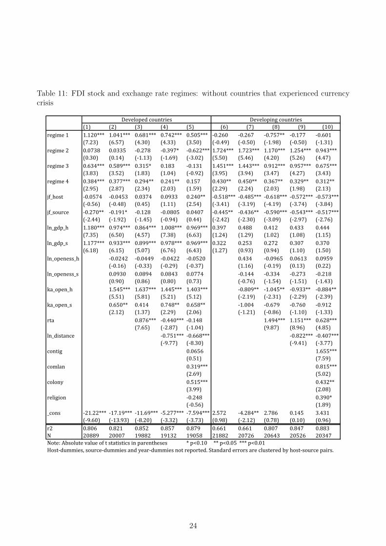
Table 11: FDI stock and exchange rate regimes: without countries that experienced currencycrisis

(1) (2) (3) (4) (5) (6) (7) (8) (9) (10)

regime 1 1.120*** 1.041*** 0.681*** 0.742*** 0.505*** -0.260 -0.267 -0.757** -0.177 -0.601

(7.23) (6.57) (4.30) (4.33) (3.50) (-0.49) (-0.50) (-1.98) (-0.50) (-1.31)

regime 2 0.0738 0.0335 -0.278 -0.397* -0.622*** 1.724*** 1.723*** 1.170*** 1.254*** 0.943***

(0.30) (0.14) (-1.13) (-1.69) (-3.02) (5.50) (5.46) (4.20) (5.26) (4.47)

regime 3 0.634*** 0.589*** 0.315* 0.183 -0.131 1.451*** 1.443*** 0.912*** 0.957*** 0.675***

(3.83) (3.52) (1.83) (1.04) (-0.92) (3.95) (3.94) (3.47) (4.27) (3.43)

regime 4 0.384*** 0.377*** 0.294** 0.241** 0.157 0.430** 0.450** 0.367** 0.329** 0.312**

(2.95) (2.87) (2.34) (2.03) (1.59) (2.29) (2.24) (2.03) (1.98) (2.13)

jf_host -0.0574 -0.0453 0.0374 0.0933 0.240** -0.518*** -0.485*** -0.618*** -0.572*** -0.573***

(-0.56) (-0.48) (0.45) (1.11) (2.54) (-3.41) (-3.19) (-4.19) (-3.74) (-3.84)

jf_source -0.270** -0.191* -0.128 -0.0805 0.0407 -0.445** -0.436** -0.590*** -0.543*** -0.517***

(-2.44) (-1.92) (-1.45) (-0.94) (0.44) (-2.42) (-2.30) (-3.09) (-2.97) (-2.76)

ln_gdp_h 1.180*** 0.974*** 0.864*** 1.008*** 0.969*** 0.397 0.488 0.412 0.433 0.444

(7.35) (6.50) (4.57) (7.38) (6.63) (1.24) (1.29) (1.02) (1.08) (1.15)

ln_gdp_s 1.177*** 0.933*** 0.899*** 0.978*** 0.969*** 0.322 0.253 0.272 0.307 0.370

(6.18) (6.15) (5.07) (6.76) (6.43) (1.27) (0.93) (0.94) (1.10) (1.50)

ln_openess_h -0.0242 -0.0449 -0.0422 -0.0520 0.434 -0.0965 0.0613 0.0959

(-0.16) (-0.33) (-0.29) (-0.37) (1.16) (-0.19) (0.13) (0.22)

ln_openess_s 0.0930 0.0894 0.0843 0.0774 -0.144 -0.334 -0.273 -0.218

(0.90) (0.86) (0.80) (0.73) (-0.76) (-1.54) (-1.51) (-1.43)

ka_open_h 1.545*** 1.637*** 1.445*** 1.403*** -0.809** -1.045** -0.933** -0.884**

(5.51) (5.81) (5.21) (5.12) (-2.19) (-2.31) (-2.29) (-2.39)

ka_open_s 0.650** 0.414 0.748** 0.658** -1.004 -0.679 -0.760 -0.912

(2.12) (1.37) (2.29) (2.06) (-1.21) (-0.86) (-1.10) (-1.33)

rta 0.876*** -0.440*** -0.148 1.494*** 1.151*** 0.628***

(7.65) (-2.87) (-1.04) (9.87) (8.96) (4.85)

ln_distance -0.751*** -0.668*** -0.822*** -0.407***

(-9.77) (-8.30) (-9.41) (-3.77)

contig 0.0656 1.655***

(0.51) (7.59)

comlan 0.319*** 0.815***

(2.69) (5.02)

colony 0.515*** 0.432**

(3.99) (2.08)

religion -0.248 0.390*

(-0.56) (1.89)

_cons -21.22*** -17.19*** -11.69*** -5.277*** -7.594*** 2.572 -4.284** 2.786 0.145 3.431

(-9.60) (-13.93) (-8.20) (-3.32) (-3.73) (0.98) (-2.12) (0.78) (0.10) (0.96)

r2 0.806 0.821 0.852 0.857 0.879 0.661 0.661 0.807 0.847 0.883

N 20889 20007 19882 19132 19058 21882 20726 20643 20526 20347

Note: Absolute value of t statistics in parentheses * p<0.10 ** p<0.05 *** p<0.01

Host-dummies, source-dummies and year-dummies not reported. Standard errors are clustered by host-source pairs.

Developed countries Developing countries

24

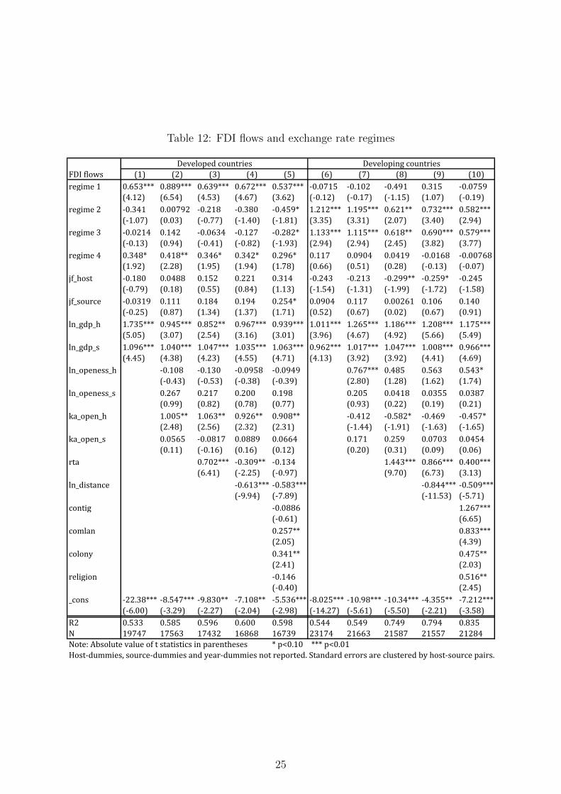
Table 12: FDI flows and exchange rate regimes

FDI flows (1) (2) (3) (4) (5) (6) (7) (8) (9) (10)

regime 1 0.653*** 0.889*** 0.639*** 0.672*** 0.537*** -0.0715 -0.102 -0.491 0.315 -0.0759

(4.12) (6.54) (4.53) (4.67) (3.62) (-0.12) (-0.17) (-1.15) (1.07) (-0.19)

regime 2 -0.341 0.00792 -0.218 -0.380 -0.459* 1.212*** 1.195*** 0.621** 0.732*** 0.582***

(-1.07) (0.03) (-0.77) (-1.40) (-1.81) (3.35) (3.31) (2.07) (3.40) (2.94)

regime 3 -0.0214 0.142 -0.0634 -0.127 -0.282* 1.133*** 1.115*** 0.618** 0.690*** 0.579***

(-0.13) (0.94) (-0.41) (-0.82) (-1.93) (2.94) (2.94) (2.45) (3.82) (3.77)

regime 4 0.348* 0.418** 0.346* 0.342* 0.296* 0.117 0.0904 0.0419 -0.0168 -0.00768

(1.92) (2.28) (1.95) (1.94) (1.78) (0.66) (0.51) (0.28) (-0.13) (-0.07)

jf_host -0.180 0.0488 0.152 0.221 0.314 -0.243 -0.213 -0.299** -0.259* -0.245

(-0.79) (0.18) (0.55) (0.84) (1.13) (-1.54) (-1.31) (-1.99) (-1.72) (-1.58)

jf_source -0.0319 0.111 0.184 0.194 0.254* 0.0904 0.117 0.00261 0.106 0.140

(-0.25) (0.87) (1.34) (1.37) (1.71) (0.52) (0.67) (0.02) (0.67) (0.91)

ln_gdp_h 1.735*** 0.945*** 0.852** 0.967*** 0.939*** 1.011*** 1.265*** 1.186*** 1.208*** 1.175***

(5.05) (3.07) (2.54) (3.16) (3.01) (3.96) (4.67) (4.92) (5.66) (5.49)

ln_gdp_s 1.096*** 1.040*** 1.047*** 1.035*** 1.063*** 0.962*** 1.017*** 1.047*** 1.008*** 0.966***

(4.45) (4.38) (4.23) (4.55) (4.71) (4.13) (3.92) (3.92) (4.41) (4.69)

ln_openess_h -0.108 -0.130 -0.0958 -0.0949 0.767*** 0.485 0.563 0.543*

(-0.43) (-0.53) (-0.38) (-0.39) (2.80) (1.28) (1.62) (1.74)

ln_openess_s 0.267 0.217 0.200 0.198 0.205 0.0418 0.0355 0.0387

(0.99) (0.82) (0.78) (0.77) (0.93) (0.22) (0.19) (0.21)

ka_open_h 1.005** 1.063** 0.926** 0.908** -0.412 -0.582* -0.469 -0.457*

(2.48) (2.56) (2.32) (2.31) (-1.44) (-1.91) (-1.63) (-1.65)

ka_open_s 0.0565 -0.0817 0.0889 0.0664 0.171 0.259 0.0703 0.0454

(0.11) (-0.16) (0.16) (0.12) (0.20) (0.31) (0.09) (0.06)

rta 0.702*** -0.309** -0.134 1.443*** 0.866*** 0.400***

(6.41) (-2.25) (-0.97) (9.70) (6.73) (3.13)

ln_distance -0.613*** -0.583*** -0.844*** -0.509***

(-9.94) (-7.89) (-11.53) (-5.71)

contig -0.0886 1.267***

(-0.61) (6.65)

comlan 0.257** 0.833***

(2.05) (4.39)

colony 0.341** 0.475**

(2.41) (2.03)

religion -0.146 0.516**

(-0.40) (2.45)

_cons -22.38*** -8.547*** -9.830** -7.108** -5.536*** -8.025*** -10.98*** -10.34*** -4.355** -7.212***

(-6.00) (-3.29) (-2.27) (-2.04) (-2.98) (-14.27) (-5.61) (-5.50) (-2.21) (-3.58)

R2 0.533 0.585 0.596 0.600 0.598 0.544 0.549 0.749 0.794 0.835

N 19747 17563 17432 16868 16739 23174 21663 21587 21557 21284

Note: Absolute value of t statistics in parentheses * p<0.10 *** p<0.01

Host-dummies, source-dummies and year-dummies not reported. Standard errors are clustered by host-source pairs.

Developed countries Developing countries

25