GEOLOGIAN TUTKIMUSKESKUS ESY/Merigeologia ja geofysiikka Espoo 47/2011

Characterization of geotomographic studies with the EMRE system

Arto Korpisalo

GEOLOGIAN TUTKIMUSKESKUS ESY/Merigeologia ja geofysiikka Espoo 47/2011

GEOLOGIAN TUTKIMUSKESKUS

GEOLOGIAN TUTKIMUSKESKUS KUVAILULEHTI Päivämäärä / Dnro

06.12.2011

Tekijät

Arto Korpisalo Raportin laji

Archive report

Toimeksiantaja

Raportin nimi Characterization of geotomographic studies with the EMRE systemTiivistelmä

The EMRE (ElectroMagnetic Radiofrequency Echoing) system consists of a continuous wave (CW) transmitter and a su-perheterodyne-type receiver. The system is designed, for example, to scan conductive mineralizations between two deep boreholes, to help in mine planning or to determine the structural integrity of the rock in the area. The method is based on the radiowave attenuation between the boreholes and is known as a radiofrequency imaging method (RIM).

The physical characteristics of geomographic feasibility studies of RIM/EMRE are presented. A short description of the behaviour of electromagnetic field has been introduced to distinguish between the real wave propagation and diffusion movement in a dissipative medium using the Q-factor. The studies on the theoretical attenuation rates of various materials are examined to identify the conditions under which the sufficient penetration distances can be achieved. The results indicate that the transillumination distances can be up to 1000 metres in highly resistive environment at the lowest measurement fre-quency of the system (312.5 kHz), at least. The cross-sectional image or tomographic reconstruction of the borehole section is based on the far-field approximation of the electric field when the field is assumed to propagate along straight rays from the source to the receiver and the changes in the electromagnetic field are generated by the changes in the material properties along the ray. The special purpose methods (ART, SIRT) are included in the commercial software called ImageWin which are the traditional methods to solve the reconstruction problem. The field surveys were conducted at Olkiluoto in western Finland. The estimated apparent resistivities ranged between tens and tens of thousands of Ωm. The first results indicate that RIM can really be a potential geophysical method. The measurement technique is simple. The step size of the transmitter can be equal to the length of transmitter antenna due to the dense measurement sequence of the receiver. Quick considerations for the geology of the borehole section can already be done by investigating the real time signals on the laptop. The final interpretation is done quickly using the traditional methods and can give good results, especially when the electrical contrasts are moderate. Asiasanat (kohde, menetelmät jne.)

electromagnetic, radiofrequency imaging method, RIM, ElectroMagnetic Radiofrequency Echoing, EMRE, cross-borehole geophysics, ART, SIRT, ImageWin, tomogram Maantieteellinen alue (maa, lääni, kunta, kylä, esiintymä)

Karttalehdet

Muut tiedot

Arkistosarjan nimi

Arkistotunnus

46/2011 Kokonaissivumäärä

47Kieli Hinta Julkisuus

julkinenYksikkö ja vastuualue

ESY/Merigeologia ja geofysiikka Hanketunnus

7780061 Allekirjoitus/nimen selvennys

Arto Korpisalo Allekirjoitus/nimen selvennys

GEOLOGIAN TUTKIMUSKESKUS 6.6.2012

Sisällysluettelo

1 INTRODUCTION .............................................................................................................................................. 1

2 THEORY ............................................................................................................................................................. 3

3 RIM INSTRUMENT ....................................................................................................................................... 19

4 MEASUREMENT TECHNIQUE AND SYSTEM CAPACITIES ................................................................ 23

5 PROCESSING AND INTERPRETATION ................................................................................................... 29

6 FIELD CASE IN FINLAND ............................................................................................................................ 34

7 DISCUSSION AND CONCLUSIONS ............................................................................................................ 39

8 REFERENCES .................................................................................................................................................. 45

1

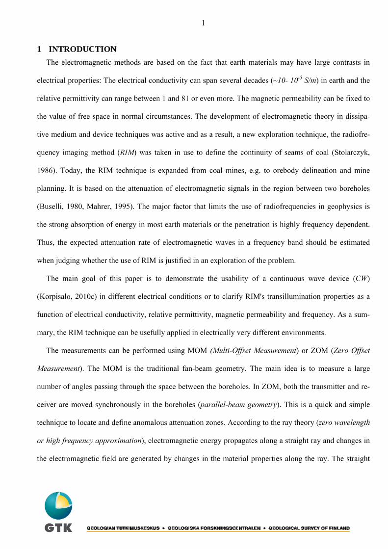
1 INTRODUCTION The electromagnetic methods are based on the fact that earth materials may have large contrasts in

electrical properties: The electrical conductivity can span several decades (~10- 10-5 S/m) in earth and the

relative permittivity can range between 1 and 81 or even more. The magnetic permeability can be fixed to

the value of free space in normal circumstances. The development of electromagnetic theory in dissipa-

tive medium and device techniques was active and as a result, a new exploration technique, the radiofre-

quency imaging method (RIM) was taken in use to define the continuity of seams of coal (Stolarczyk,

1986). Today, the RIM technique is expanded from coal mines, e.g. to orebody delineation and mine

planning. It is based on the attenuation of electromagnetic signals in the region between two boreholes

(Buselli, 1980, Mahrer, 1995). The major factor that limits the use of radiofrequencies in geophysics is

the strong absorption of energy in most earth materials or the penetration is highly frequency dependent.

Thus, the expected attenuation rate of electromagnetic waves in a frequency band should be estimated

when judging whether the use of RIM is justified in an exploration of the problem.

The main goal of this paper is to demonstrate the usability of a continuous wave device (CW)

(Korpisalo, 2010c) in different electrical conditions or to clarify RIM's transillumination properties as a

function of electrical conductivity, relative permittivity, magnetic permeability and frequency. As a sum-

mary, the RIM technique can be usefully applied in electrically very different environments.

The measurements can be performed using MOM (Multi-Offset Measurement) or ZOM (Zero Offset

Measurement). The MOM is the traditional fan-beam geometry. The main idea is to measure a large

number of angles passing through the space between the boreholes. In ZOM, both the transmitter and re-

ceiver are moved synchronously in the boreholes (parallel-beam geometry). This is a quick and simple

technique to locate and define anomalous attenuation zones. According to the ray theory (zero wavelength

or high frequency approximation), electromagnetic energy propagates along a straight ray and changes in

the electromagnetic field are generated by changes in the material properties along the ray. The straight

2

ray assumption is valid in moderate contrasts when the reconstructed tomographic images can also be re-

liable. Only the waves that propagate in the first Fresnel zone (e.g. direct and multipath waves) are gener-

ally strong enough and detectable. In addition, the smallest structure that can be resolved, can be estimat-

ed by the width of the first Fresnel zone. The performance level of the EMRE system (maximum distanc-

es rmax) is estimated using a simplified model (Pralat & Zdunek, 2005). Our conclusion is that the maxi-

mum borehole distances can be up to 1000 metres.

When the amplitude data is collected, it is the attenuation that can be estimated directly. Because the

impedance of transmitter antenna and the gains are unknown in the EMRE system, the Friis transmission

equation is not usable. But using a plane wave assumption, which is valid in the far-field, the measured

amplitudes can be converted to the attenuation distribution in a simple way. Olkiluoto served as a testing

place for the RIM measurements to determine the capacity and usefulness of RIM in determining the

structural integrity of the rock in the area. Despite a challenging measurement geometry and the sulphide-

rich areas in the bedrock, the measurements and results were successful and good. However, the smaller

scaled fractures couldn't be separated in the conductive rock mass.

After the positive experiences with RIM, the renovation of the EMRE system is under considerations.

The highest frequency can be increased to 5000 kHz. The sensitivity and the angular resolution of the re-

ceiver can be improved by new solutions. In addition, to improve the operation level of the receiver, the

present mixer technique must be modernized, followed by an effective filter stages. With developments of

this kind, the EMRE system could become a powerful tool in large rock building projects to more precise-

ly determine the structural integrity of the rock. The relative phase difference contains information on the

relative permittivity. Thus, the development of phase interpretation is also under consideration.

3

2 THEORY A cross-borehole EM survey has several clear benefits over ground- level electromagnetic sounding

methods. Applying a borehole transmitter, brings the survey closer to the target, and will allow the use of

higher frequencies, thus enabling a higher spatial resolution. Another benefit is the possibility to view the

target from different angles and directions not only in the vertical direction. Having the transmitter in a

borehole, eliminates the boundary effects related to the ground surface and the strong attenuation emerg-

ing from soil deposits. A drawback is the suboptimal availability and location of boreholes and limited

power of transmission of borehole probes. Thus, the relatively complex behaviour of a 3D source field

within the subsurface target is difficult to resolve numerically without significant approximations. The

physical behaviour of an electromagnetic field is governed mathematically by Maxwell equations, which

describe the relationship between electric and magnetic fields in a medium and quantify the material

properties. (Korpisalo, 2010c).

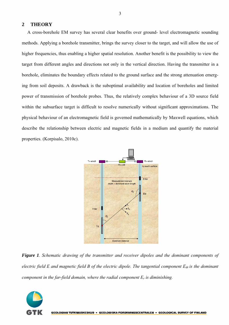
Figure 1. Schematic drawing of the transmitter and receiver dipoles and the dominant components of

electric field E and magnetic field B of the electric dipole. The tangential component EΘ is the dominant

component in the far-field domain, where the radial component Er is diminishing.

4

In the EMRE system, the electromagnetic fields are generated by insulated electric dipole antennas

(Korpisalo, 2010a) that are aligned parallel to the borehole axis. Figure 1 presents the separation of elec-

tromagnetic field of the electric dipole into its effective components: a magnetic component (B φ) and an

electric tangential component (EΘ) and radial component (Er). The electric field determines the polariza-

tion, and the maximal coupling with targets is achieved when the field component is parallel to the target.

The major factor that limits the use of radiofrequencies in geophysics is the strong absorption of energy in

most earth materials or the penetration is highly frequency dependent. Thus, the expected attenuation rate

of electromagnetic waves in a frequency band should be estimated when judging whether the use of RIM

is justified in an exploration of the problem.

The field depends on the distance r from the source. Certain characteristics of an electromagnetic

field dominates at one particular distance from the antenna, while a completely different behaviour can

dominate at another location. The wave number k multiplied by the distance r , defines the behaviour

(Korpisalo, 2010a). When rk ⋅ <<1 or at a distance much shorter than the wavelength, the electric field

resembles the static dipole field being proportional to r–3 (static term), and anything in this region that

couples with the antenna will disturb the antenna severely (reactive near-field). The EMRE system oper-

ates in the near-field domain due to the wavelengths of hundreds of metres when low frequencies (f < 300

kHz) and short distances (r < 50 m) are used in a resistivity range of <1000 Ωm. When rk ⋅ =1, the field

is proportional to r–2 (induction term), and the static and induction terms (~r-2, r-3) become negligible. The

region is known as a radiating near-field or Fresnel zone. At the frequency range of 300–2500 kHz and

with resistivities <10 000 Ωm, the EMRE system operates in the radiating domain. When rk ⋅ >>1 or at a

distance much greater than the wavelength, the electric field is inversely dependent on the distance r-1

(radiation term). The angular field distribution is independent of the distance from the antenna (far-field

5

or Fraunhofer zone). When frequencies f > 1000 kHz and distances r > 100 m are used in the resistivity

range of >10 000 Ωm, the EMRE system is operating in the far-field.

The inhomogeneous generalized time-domain wave equations for the time harmonic electric field E

and magnetic field H (eiωt dependence) can be written as (Korpisalo, 2010c)

tJ

tE

dtEE

∂∂

+∇=∂

∂−

∂−∇ μρ

εμεμσ 1

2

22 (1)

JtH

dtHH ×−∇=

∂

∂−

∂−∇ 2

22 μεμσ (2)

On the right-hand side are the sources of the fields. On the left-hand side, the second-order time-

derivative term is the wave term (oscillating term) with an energy storage factor (με) and the first-order

time-derivative term is the damping term with an energy dissipation factor (μσ). For sinusoidal time-

harmonic fields (~eiωt), these equations (in a source-free region, ρ = 0 and J = 0) become frequency-

domain Helmholtz's equations by using the following substitutions; 22

2 , ωω −→∂

∂→

∂∂

ti

t

00 2222 =+∇→=+−∇ EkEEEiE μεωωμσ (3)

00 2222 =+∇→=+−∇ EkEHHiH μεωωμσ

ωμσμεω ik −= 22

(4)

where is the complex wave number (Korpisalo, 2010c). Depending on the magnitude of energy loss (conductivity) relative to energy storage (permittivity, perme-

ability), the fields may diffuse or propagate as waves. The Q-factor (inverse loss tangent) describes the

behaviour of the field (Daniels, 1996),

σεω

εωσσεω

εωσωσε

′′

≈Φ=′′+′′′−′

=′′+′

′′−′= −1tan/Q

σ ′′ σσσ ′′+′= i ε ′′ εεε ′′+′= i

(5)

In its effective form (Eq. 5), the Q-factor contains the imaginary components of complex conductivity

( ) and permittivity ( ). The loss tangent of any material (tanφ) quantita-

6

tively describes dissipation of the electric energy due to different physical processes such as electrical

conduction, dielectric relaxation, dielectric resonance and loss from nonlinear processes (hysteresis).

When Q >> 1 (high frequency/low conductivity), the dielectric properties are dominant ( ),

and the electromagnetic fields propagate as waves through the medium. All the frequency components

travel roughly at the same velocity (non–dispersive), encounter the same negligible attenuation α and the

waveform remains unaltered through the passage. Reflection, scattering, refraction and diffraction effects

on the boundaries are possible due to the different electrical properties, resulting, for instance, in multi-

path waves. The velocity v, attenuation rate α, phase shift β, wave impedance η and wave number k can

be written as

σεω ′>>′

εμ1

=v Ω≈= 377εμη (6)

2σ

εμα ⋅= μεωβ = μεω22 =k

ε

σεω ′<<′

(7)

The attenuation rate is dependent on the dielectric permittivity , magnetic permeability µ and electrical

conductivity σ, but not on the frequency ω. The phase shift is dependent on the frequency, permittivity

and permeability. When σ = 0, the wave impedance has the value of a vacuum or η ≈ 377 Ω. The wave

impedance is an important factor when reflection and transmission coefficients are concerned in the

boundaries.

When Q << 1 ( ), the velocity v is independent of the dielectric permittivity ε (quasi-static),

but is controlled by the product of conductivity σ and permeability µ. The energy distribution is disper-

sive, i.e. the attenuation α will depend on the conductivity σ, permeability µ and frequency ω

μσω2

=v ( ) )4/(12

πσ

ωμσ

ωμσωμη ieii

=+==

ωμσik −=2

(8)

. βδ

ωμσα ===1

2 (9)

7

Thus, the phase shift is equal to the attenuation constant (Eq. 9). One wavelength λ means a phase shift of

2π radians. It is also the distance corresponding to 2π Nepers (~55 dB) of attenuation (1 Neper = 8.686

dB). In addition, one skin depth, a distance where the field has attenuated to e–1 of the initial field

strength, means an attenuation of 1 Neper (~9 dB), corresponding to one radian length (~57o). In the low

Q-domain, the attenuation is equal to the phase shift and can be described in terms of skin depth δ (Eq. 9).

The skin depth is a plane wave factor that is attached to damping fields. The induced volume currents can

be replaced by the surface currents and the current is concentrated on the surface of the target. The ap-

proximation holds both in the high frequency domain, when the conductivity has to be large enough, and

in the low frequency domain, when the target can be more resistive. In conductors, the wave impedance is

complex valued. Thus, the electric and magnetic fields are no longer in phase (Eq. 8). For almost all

rocks, the magnetic susceptibility χm << 1 (μr = 1+χm), thus, the permeability μ ≅ μo or μr = 1. In the wave

equations (Eqs. 1-2), the permeability μ appears as a product with conductivity σ (μσ). Due to the large

range of conductivity variation in the Earth's materials (~10 - 10-5 S/m), the conductivity outweighs the

permeability changes (μr≈1). However, it is evident that the effect of increasing the permeability is to in-

crease the attenuation and phase shift. In quasi-static conditions (diffusive domain), electromagnetic fields

don’t experience the above-mentioned effects on the boundaries (e.g. reflection, refractions), but the

fields diffuse over the boundaries like heat.

When Q ≈ 1 ( ,Figs. 2- 3), the system is in the intermediate domain where

both the electric permittivity and conductivity and permeability influence the phase shift and attenuation

rate. To estimate the phase shift (β) and attenuation rate (α) in a dissipative medium, more general ex-

pressions must be used for the phase and attenuation constants

σεω ↔′≅′ επσ ′′≈ 2/f

)/(1tan12

112

2/12

2/12

mrad⎟⎠⎞⎜

⎝⎛ +Φ+=

⎟⎟⎟

⎠

⎞

⎜⎜⎜

⎝

⎛+⎟

⎠⎞

⎜⎝⎛+=

μεωωεσμεωβ (10)

8

)/(1tan12

*686.8112

*686.82/1

22/1

2mdB⎟

⎠⎞⎜

⎝⎛ −Φ+=

⎟⎟⎟

⎠

⎞

⎜⎜⎜

⎝

⎛−⎟

⎠⎞

⎜⎝⎛+=

μεωωεσμεωα

.

The phase velocity v, the wavelength λ and wave number k for a dissipative medium are obtained using

the following general formulas:

2/12

2/12 1tan12

1

112

1

⎟⎠⎞⎜

⎝⎛ +Φ+

=

⎟⎟⎟

⎠

⎞

⎜⎜⎜

⎝

⎛+⎟

⎠⎞

⎜⎝⎛+

==

μεω

ωεσ

μεω

βω

pv

2/12

2/12

1tan12111212 −−

⎟⎠⎞⎜

⎝⎛ +Φ+=

⎟⎟⎟

⎠

⎞

⎜⎜⎜

⎝

⎛+⎟

⎠⎞

⎜⎝⎛+==

μεωεσ

μεβπλ

ff

ωμσμεω ik −= 22

πωσ 2/′

. (11)

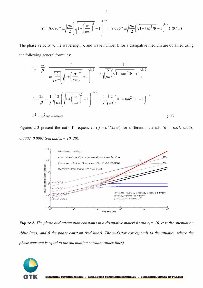
Figures 2-3 present the cut-off frequencies ( ) for different materials (σ = 0.01, 0.001,

0.0002, 0.0001 S/m and εr = 10, 20).

=f

Figure 2. The phase and attenuation constants in a dissipative material with εr = 10, α is the attenuation

(blue lines) and β the phase constant (red lines). The m-factor corresponds to the situation where the

phase constant is equal to the attenuation constant (black lines).

9

In a fairly conductive rock (σ = 0.01S/m, εr = 10), the quasi-static conditions (displacement current neg-

ligible) are valid almost up to ~1000 kHz, while in a highly resistive environment (σ = 0.0001 S/m), the

quasi-static conditions are valid up to ~10 kHz (Fig. 2).

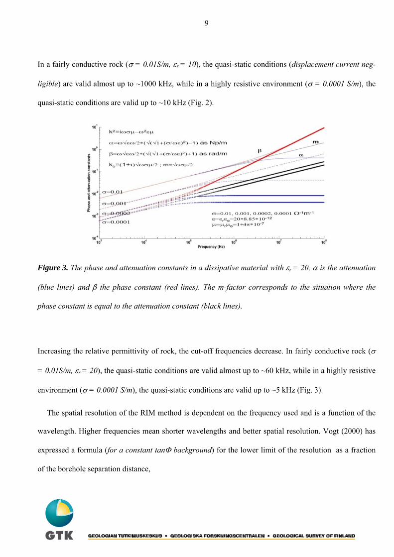
Figure 3. The phase and attenuation constants in a dissipative material with εr = 20, α is the attenuation

(blue lines) and β the phase constant (red lines). The m-factor corresponds to the situation where the

phase constant is equal to the attenuation constant (black lines).

Increasing the relative permittivity of rock, the cut-off frequencies decrease. In fairly conductive rock (σ

= 0.01S/m, εr = 20), the quasi-static conditions are valid almost up to ~60 kHz, while in a highly resistive

environment (σ = 0.0001 S/m), the quasi-static conditions are valid up to ~5 kHz (Fig. 3).

The spatial resolution of the RIM method is dependent on the frequency used and is a function of the

wavelength. Higher frequencies mean shorter wavelengths and better spatial resolution. Vogt (2000) has

expressed a formula (for a constant tanΦ background) for the lower limit of the resolution as a fraction

of the borehole separation distance,

10

24 R⋅⋅π10max

21

2

2

210max

21

2

2

log10686.82

1tan1

1tan14log10

686.82

11

11

bRbR ⋅−

⋅⋅⎥⎥⎦

⎤

⎢⎢⎣

⎡

+Φ+

−Φ+=

⋅⋅⋅−

⋅⋅

⎥⎥⎥⎥⎥

⎦

⎤

⎢⎢⎢⎢⎢

⎣

⎡

+⎟⎠⎞

⎜⎝⎛+

−⎟⎠⎞

⎜⎝⎛+

=π

ππ

ωεσ

ωεσ

λ

(12)

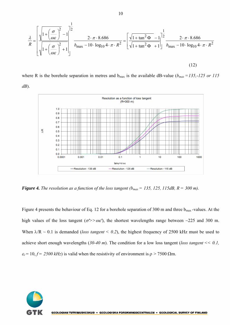
where R is the borehole separation in metres and bmax is the available dB-value (bmax =135,-125 or 115

dB).

Figure 4. The resolution as a function of the loss tangent (bmax = 135, 125, 115dB, R = 300 m).

Figure 4 presents the behaviour of Eq. 12 for a borehole separation of 300 m and three bmax -values. At the

high values of the loss tangent (σ'>>ωε'), the shortest wavelengths range between ~225 and 300 m.

When λ/R ~ 0.1 is demanded (loss tangent < 0.2), the highest frequency of 2500 kHz must be used to

achieve short enough wavelengths (30-40 m). The condition for a low loss tangent (loss tangent << 0.1,

εr = 10, f = 2500 kHz) is valid when the resistivity of environment is ρ > 7500 Ωm.

11

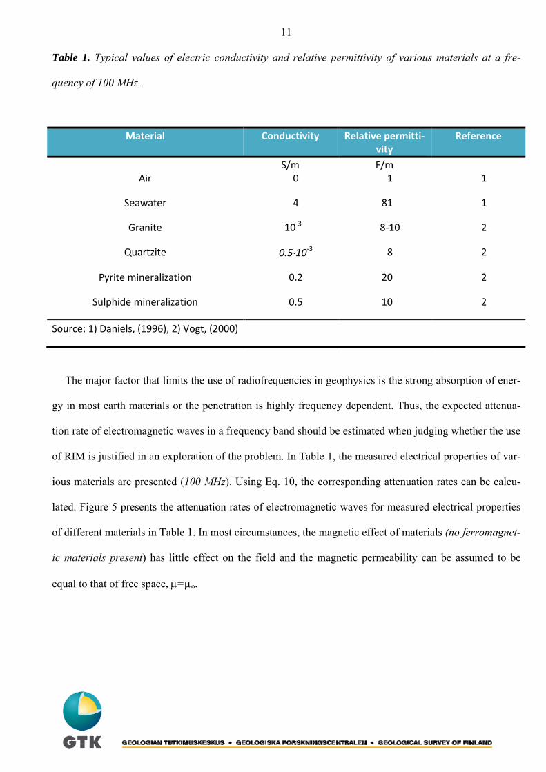
Table 1. Typical values of electric conductivity and relative permittivity of various materials at a fre-

quency of 100 MHz.

Material Conductivity Relative permitti‐vity

Reference

S/m F/m Air 0 1 1

Seawater 4 81 1

Granite 10‐3 8‐10 2

Quartzite 0.5⋅10‐3 8 2

Pyrite mineralization 0.2 20 2

Sulphide mineralization 0.5 10 2

Source: 1) Daniels, (1996), 2) Vogt, (2000)

The major factor that limits the use of radiofrequencies in geophysics is the strong absorption of ener-

gy in most earth materials or the penetration is highly frequency dependent. Thus, the expected attenua-

tion rate of electromagnetic waves in a frequency band should be estimated when judging whether the use

of RIM is justified in an exploration of the problem. In Table 1, the measured electrical properties of var-

ious materials are presented (100 MHz). Using Eq. 10, the corresponding attenuation rates can be calcu-

lated. Figure 5 presents the attenuation rates of electromagnetic waves for measured electrical properties

of different materials in Table 1. In most circumstances, the magnetic effect of materials (no ferromagnet-

ic materials present) has little effect on the field and the magnetic permeability can be assumed to be

equal to that of free space, μ=μo.

12

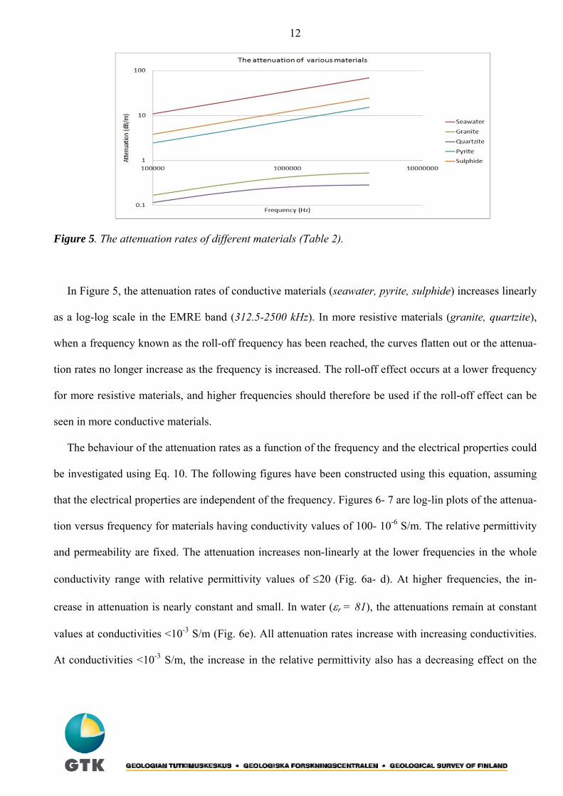
Figure 5. The attenuation rates of different materials (Table 2).

In Figure 5, the attenuation rates of conductive materials (seawater, pyrite, sulphide) increases linearly

as a log-log scale in the EMRE band (312.5-2500 kHz). In more resistive materials (granite, quartzite),

when a frequency known as the roll-off frequency has been reached, the curves flatten out or the attenua-

tion rates no longer increase as the frequency is increased. The roll-off effect occurs at a lower frequency

for more resistive materials, and higher frequencies should therefore be used if the roll-off effect can be

seen in more conductive materials.

The behaviour of the attenuation rates as a function of the frequency and the electrical properties could

be investigated using Eq. 10. The following figures have been constructed using this equation, assuming

that the electrical properties are independent of the frequency. Figures 6- 7 are log-lin plots of the attenua-

tion versus frequency for materials having conductivity values of 100- 10-6 S/m. The relative permittivity

and permeability are fixed. The attenuation increases non-linearly at the lower frequencies in the whole

conductivity range with relative permittivity values of ≤20 (Fig. 6a- d). At higher frequencies, the in-

crease in attenuation is nearly constant and small. In water (εr = 81), the attenuations remain at constant

values at conductivities <10-3 S/m (Fig. 6e). All attenuation rates increase with increasing conductivities.

At conductivities <10-3 S/m, the increase in the relative permittivity also has a decreasing effect on the

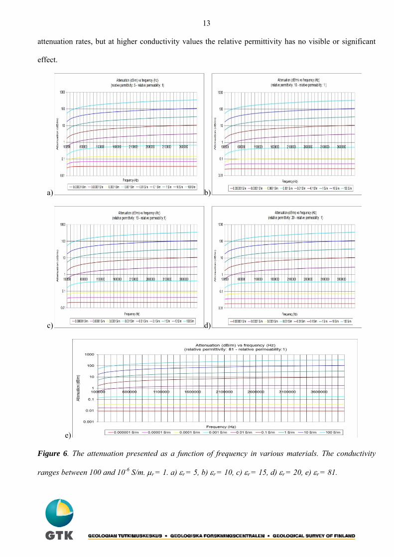
13

attenuation rates, but at higher conductivity values the relative permittivity has no visible or significant

effect.

a) b)

c) d)

e)

Figure 6. The attenuation presented as a function of frequency in various materials. The conductivity

ranges between 100 and 10-6 S/m. μr = 1. a) εr = 5, b) εr = 10, c) εr = 15, d) εr = 20, e) εr = 81.

14

a)

b)

c)

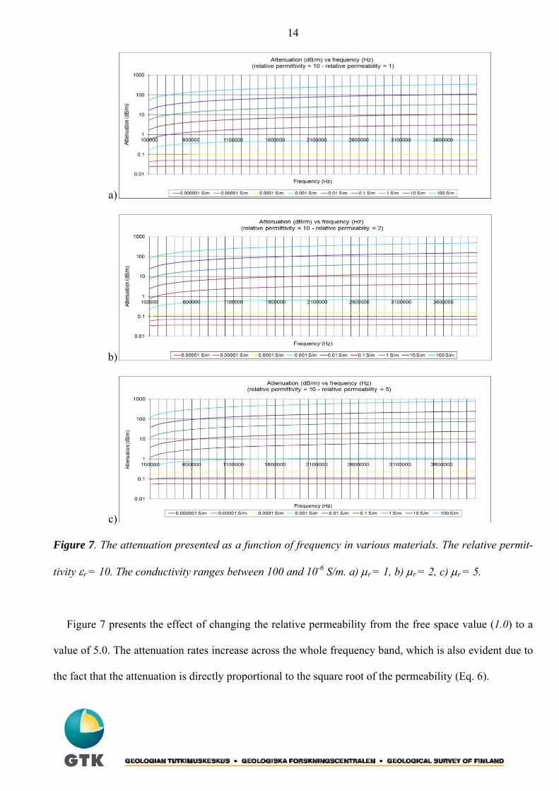
Figure 7. The attenuation presented as a function of frequency in various materials. The relative permit-

tivity εr = 10. The conductivity ranges between 100 and 10-6 S/m. a) μr = 1, b) μr = 2, c) μr = 5.

Figure 7 presents the effect of changing the relative permeability from the free space value (1.0) to a

value of 5.0. The attenuation rates increase across the whole frequency band, which is also evident due to

the fact that the attenuation is directly proportional to the square root of the permeability (Eq. 6).

15

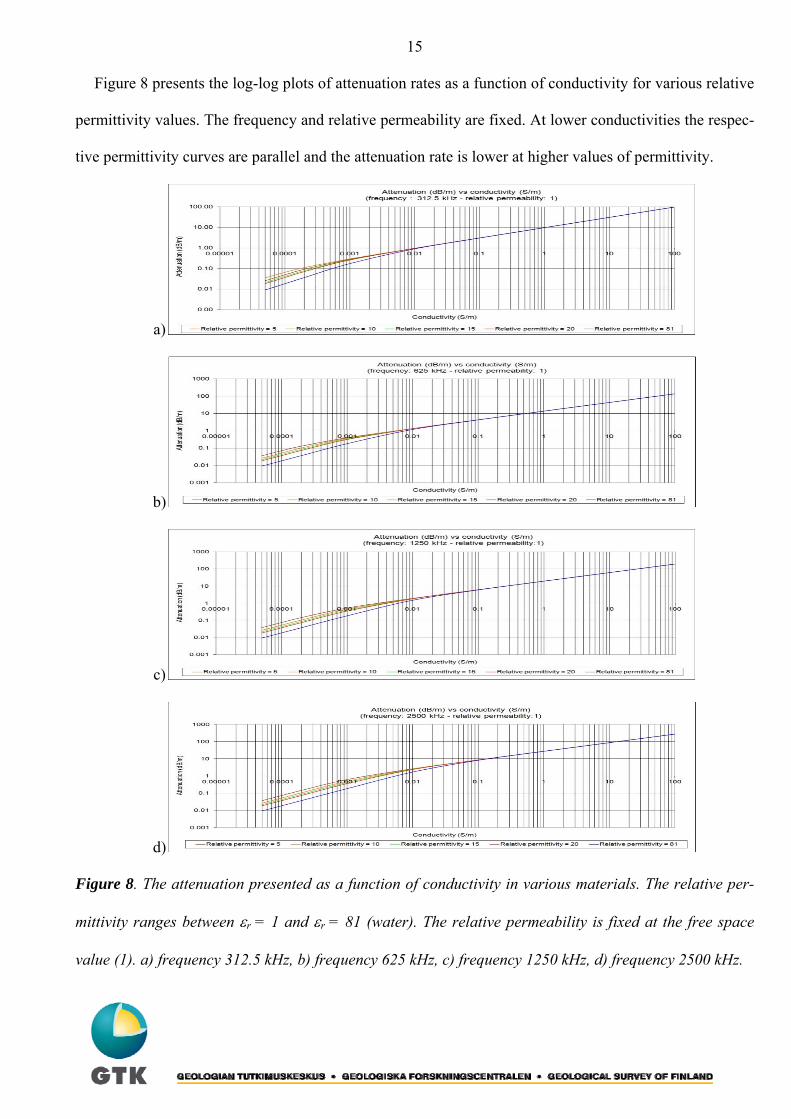
Figure 8 presents the log-log plots of attenuation rates as a function of conductivity for various relative

permittivity values. The frequency and relative permeability are fixed. At lower conductivities the respec-

tive permittivity curves are parallel and the attenuation rate is lower at higher values of permittivity.

a)

b)

c)

d)

Figure 8. The attenuation presented as a function of conductivity in various materials. The relative per-

mittivity ranges between εr = 1 and εr = 81 (water). The relative permeability is fixed at the free space

value (1). a) frequency 312.5 kHz, b) frequency 625 kHz, c) frequency 1250 kHz, d) frequency 2500 kHz.

16

In resistive materials, the attenuation is dependent on the permittivity value but at the critical conduc-

tivity values of ~10-2-10-1 S/m the curves merge together to become identical, and this happens sooner at

lower frequencies. This is clear because Eq.6 reduces to a form of μωσα eff≅ when the loss tangent is

much greater than unity. The attenuation rates increase as the conductivity increases in all plots (Fig. 8).

The attenuation rates of rocks can also be measured directly as in-situ measurements. Direct measure-

ment, in which the reduction in the amplitude of an electromagnetic wave due to a known distance of ma-

terial is measured, is the most accurate method of measuring the attenuation rate. Vogt (2000) reported a

capacitive method in which small cylindrical pieces of different rock types were carefully prepared and

placed as a dielectric in the capacitor. Thus, measuring the complex impedance of the capacitor, the elec-

trical conductivity σ and the relative permittivity εr of the sample could be calculated. The reliability of

the results is not good, because the electrical properties are highly variable. For instance, the moisture of

sample is probably changed and it is always a question about a certain scale dependence in which differ-

ent factors are involved: in-situ measurements represent an average over a much larger rock volume than

laboratory measurements performed on small samples. On the other hand, small-scale variations may thus

be lost in in-situ measurements. . Thus, the results may not even reflect the properties in-situ. When the

measured conductivities and permittivities are concerned, the conductivity must be introduced in a form

and the permittivity in a form of , where and are the imaginary

parts of complex conductivity (dielectric conductivity) and permittivity (conductive permittivity). The die-

lectric conductivity takes account of time lags in conduction and the conductive permittivity

takes account of time lags in polarization. Generally, the separation of measured values of the conductivi-

ty and permittivity into their complex components is a complicated problem. Dr D. Vogt performed and

published Vector Impedance Meter– measurements of the electrical properties of different rock types in

the frequency range of 1-64 MHz (Vogt, 2000). The results from two samples and the corresponding De-

bye models (multiple relaxation times) are plotted as black curves in Figure 9.

εωσσ ′′−′=eff ωσεε /′′+′=eff σ ′′ ε ′′

σ ′′ ε ′′

17

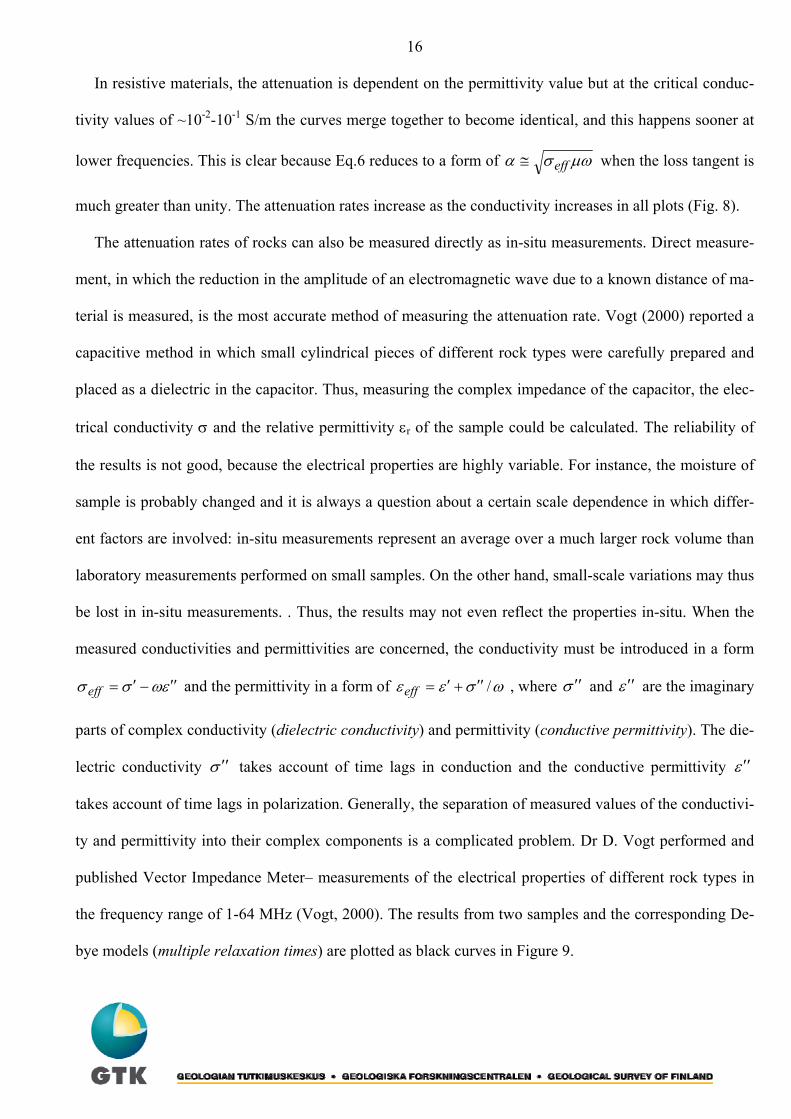
a) b)

Figure 9. The electrical properties of a granite sample (a) and a sulphide sample (b) from Vogt (2000).

Error bars are included to show the uncertainty of the measurements.

Figure 9 presents the results of capacitive measurements of two small cylindrical rock samples by Vogt

(2000) to determine the electrical conductivity and relative permittivity. The remaining properties are

generated from the measured values. The measurements include a certain degree of equipment-based in-

accuracy (e.g. sample contacts to the electrodes), and error the bars are therefore included in the plots.

Granite is a highly resistive rock type in which the effective permittivity remains almost at a constant val-

ue as a function of frequency, perhaps having a slightly decreasing trend, meaning that the dielectric con-

ductivity has a minor effect on the permittivity. The effective conductivity ( ) with a

high degree of inaccuracy, is dominated by the real component at low frequencies while at higher fre-

quencies the dielectric conductivity component , the out-off phase component, starts to dominate and

has an increasing effect on the conductivity. The attenuation rate, also infected by the inaccuracy, is low,

being ~0.02 dB/m (~ 1 MHz); thus, the translumination distances should be large. The wavelengths range

between tens and hundreds of metres. The loss tangent, strongly inflected by the inaccuracy, has a slightly

decreasing trend (Fig. 9a). Sulphide is a good conductor. The effective conductivity is almost constant

σ ′′ εωσσ ′′−′=eff

ε ′′

18

(DC-value), and the real component is therefore dominant and the dielectric conductivity component

is negligible. The permittivity has a strongly decreasing trend and is strongly inflected by the inaccuracy.

The attenuation rates increase strongly as a function of frequency. The loss tangents, inflected by the in-

accuracy, are high, meaning high attenuation rates that reduce translumination distances (Fig. 9b).

ε ′′

19

3 RIM INSTRUMENT In Finland, the radiofrequency imaging method (RIM) method has been used since the pioneering work

by A. Korpisalo in 2005 (Korpisalo et al. 2008; Heikkinen et al. 2006). The effective performance of any

radiating system depends on the characteristics of transmitter and receiver antennas, because they are the

important intermediate devices that radiate and capture the propagating electromagnetic energy

(Korpisalo, 2010a). The heart of the EMRE system is a Russian-based device (Redko et al. 2000) that

simultaneously operates at a maximum of four frequencies; 312.5,- 625,- 1250 and 2500 kHz. Thus, the

survey time is reduced by measuring all frequencies simultaneously. The amplitude of the tangential

component of the electric field (far-field approximation) and the relative phase difference are measured

along the axis of the receiver borehole. The reference signal (156.25 kHz) generated in the borehole

transmitter is essential in a tuning operation of the receiver when the receiver is locked to the reference

frequency. Without a reference signal, the detection of phase difference would be impossible, but even if

the tuning is not functioning properly, the equipment can be used to detect the amplitudes. The measure-

ments are controlled and information recorded by a laptop. The automated measurement process requires

minimal intervention by the operator. The operator can monitor the data quality from the laptop's screen

at all frequencies in real time and view previous results. This allows quick adjustments to the survey

depth range and makes easy the shortening or lengthening of the transmitter step size, and will enable de-

cisions on rapid re-measurement. The technical specifications of the EMRE system are presented in Table

2.

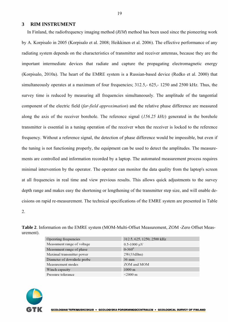
Table 2. Information on the EMRE system (MOM-Multi-Offset Measurement, ZOM -Zero Offset Meas-urement).

20

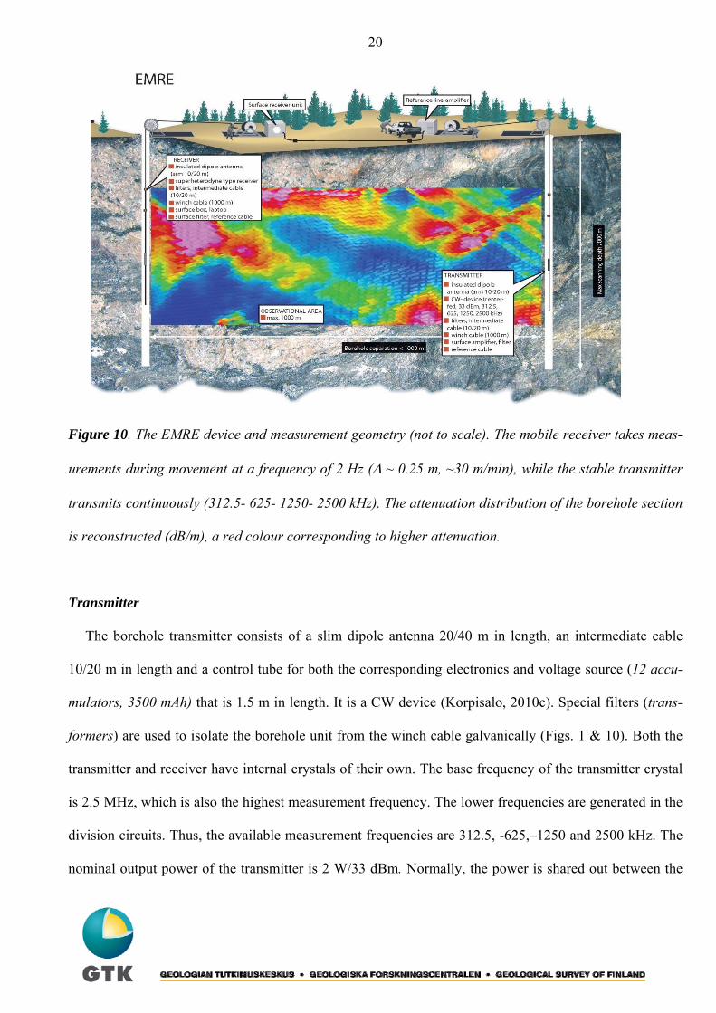
Figure 10. The EMRE device and measurement geometry (not to scale). The mobile receiver takes meas-

urements during movement at a frequency of 2 Hz (Δ ~ 0.25 m, ~30 m/min), while the stable transmitter

transmits continuously (312.5- 625- 1250- 2500 kHz). The attenuation distribution of the borehole section

is reconstructed (dB/m), a red colour corresponding to higher attenuation.

Transmitter

The borehole transmitter consists of a slim dipole antenna 20/40 m in length, an intermediate cable

10/20 m in length and a control tube for both the corresponding electronics and voltage source (12 accu-

mulators, 3500 mAh) that is 1.5 m in length. It is a CW device (Korpisalo, 2010c). Special filters (trans-

formers) are used to isolate the borehole unit from the winch cable galvanically (Figs. 1 & 10). Both the

transmitter and receiver have internal crystals of their own. The base frequency of the transmitter crystal

is 2.5 MHz, which is also the highest measurement frequency. The lower frequencies are generated in the

division circuits. Thus, the available measurement frequencies are 312.5, -625,–1250 and 2500 kHz. The

nominal output power of the transmitter is 2 W/33 dBm. Normally, the power is shared out between the

21

four frequencies. However, a frequency can be rejected from the usual operation in a special situation,

and to channel the whole power to the remaining frequencies. Because the frequencies (312-5- 2500 kHz)

are sent simultaneously, matching of the antenna impedance to the generator is impossible due to the

highly varying environmental properties (conductivity, permittivity). Thus, the effective radiative power is

diminished due to near-field losses. In addition, the high voltage standing wave ratio (VSWR) values are

evident due the open-end terminations in the antenna or a part of energy returns to the generator. The ref-

erence frequency of 156.25 kHz is sent through the winch cable to the Earth's surface. After the amplifi-

cation, it is channelled through the ground-level reference cable to the receiver box, where it is used in the

tuning operation. When a receiver tuning is accomplished, a receiver is locked to the reference frequency,

making the phase detection possible . The reference frequency is low enough to not disturb the measure-

ments (Korpisalo, 2010c).

Receiver

The borehole receiver has the same antennas and cables as the transmitter, but the control tube for the

electronics and voltage source (12 accumulators, 3500 mAh) is 2.5 m long. The galvanic isolation is per-

formed using the same types of filters as in the transmitter (Figs. 1 & 8). The receiver is established in a

manner that does not deviate from a normal radio. The front end of the receiver (RF-amplifier) and the

mixers are situated in the borehole unit. The normal components (e.g. detector where the originals are

reproduced) are situated in the surface box. Technically, it is a normal superheterodyne-type receiver in

which a long winch cable is used to transmit the modulated signals up to the detector.

The receiver has a crystal with a basic frequency of 2.6 MHz. The incoming signals are amplified and

sent to a first mixer to be heterodyned with the signals generated in the external crystal (2.6 MHz). Thus,

the IF frequencies (intermediate frequencies) of 100,-50,-25 and 12.5 kHz are generated. The band (100-

12.5 kHz) is several octaves. In the EMRE system, data is transferred from the borehole to the surface us-

22

ing a pair cable where the two filters (transformers) are connected. Because it is challenging to transfer

effectively the broad first intermediate band through the filters, another mixing stage is performed, using

the frequency of 162.5 kHz (2.6 MHz/16) to produce the second intermediate frequencies of 262.5,-

212.5, 187,5 and 175.1 kHz. This band (262.5-175.1 kHz) is not even one octave and the data transfer is

not so challenging. When the receiver has sensed a strong enough reference signal (156.25 kHz), tuning

can be performed and the receiver is ready for the proper reception. The modulated signals are fed to the

detector where both the amplitude and phase detections are performed. The digitizing is performed by a

12-bit analogue-digital converter.

The receiver has similar antennas to the transmitter. It is not compulsory to use antennas of same

lengths in transmission and reception. It is usual to use a longer antenna in transmission to make use of

the best possible efficiency and at the same time to use a shorter antenna in reception to maintain the best

possible resolution. The receiver has the same impedance mismatching problem as the transmitter and the

load (antenna) does not absorb all the RF power that reaches it. Instead, some of the RF power is sent

back towards the signal source when the signal reaches the point where the line is connected to the load.

This is known as a reflected power or reverse power. The receiver unit consists of an internal calibration

unit where the constant valued fields of 100,- 10 and 1 μV can be fed to the antenna input of the receiver.

Thus, the measured amplitude values can be converted to the actual μV-units. The receiver has a dynamic

range of ~40 dB, which can be a limiting factor. The dynamic range of a receiver is the input power range

over which the receiver is useful. Thus, the user has to select the antennas carefully in order to avoid the

saturation of the receiver. Changing the antennas, rejecting the problematic frequency or the usage of

longer distances between the transmitter and receiver are ways to eliminate saturation (Korpisalo, 2010c).

23

4 MEASUREMENT TECHNIQUE AND SYSTEM CAPACITIES According to the cross-borehole measurement geometry, the EMRE system operates in the transmis-

sion mode in order to detect the attenuation of the transmitted radiofrequency waves (Fig. 10). The meas-

urements can be performed using MOM (Multi-Offset Measurement) or ZOM (Zero Offset Measurement).

The MOM is the traditional method, whereby a stable transmitter is fixed in one borehole and a mobile

receiver is moving in the other borehole (fan-beam geometry). The main idea is to measure a large num-

ber of angles passing through the space between the boreholes. In ZOM, both the transmitter and receiver

are moved synchronously in the boreholes (parallel-beam geometry). This is a quick and simple tech-

nique to locate and define anomalous attenuation zones. In a homogeneous environment, signal levels

should be same at each location.

Two-way measurement is normally performed, where the transmitter and receiver are interchanged in

the boreholes, and a full tomographic survey can be accomplished. This is known as a limited angle

method, because the angle coverage is seldom more than 60 degrees (cf. medical computerized tomogra-

phy (CT), which has an angle coverage of 360 degrees). When the light propagates in free space, the rays

may be reflected, diffracted and scattered by the obstacles. Radiowaves may experience the same phe-

nomena when travelling through different geological deposits with quite different electrical and magnetic

properties. In addition, radiowaves suffer from strong internal attenuation. The EMRE system cannot dis-

tinguish between the above-mentioned phenomena. As a result, multipath effects (Rayleigh scattering),

for instance, are possible in the recordings. Rayleigh scattering is known as a small-scale fading effect

and is associated with small objects (order of wavelength) in the environment.

According to ray theory (zero wavelength or high frequency approximation), electromagnetic energy

propagates along a ray and changes in the electromagnetic field are generated by changes in the material

properties along the ray. In a homogeneous material, the rays are straight lines, unlike in an inhomogene-

ous material. The volume of the first Fresnel zone (prolate spheroid) is an important factor when consid-

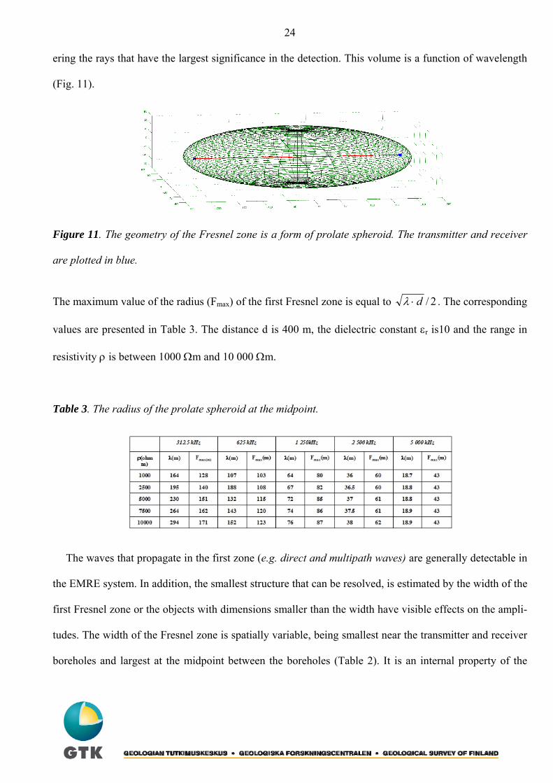
24

ering the rays that have the largest significance in the detection. This volume is a function of wavelength

(Fig. 11).

Figure 11. The geometry of the Fresnel zone is a form of prolate spheroid. The transmitter and receiver

are plotted in blue.

2/d⋅λThe maximum value of the radius (Fmax) of the first Fresnel zone is equal to . The corresponding

values are presented in Table 3. The distance d is 400 m, the dielectric constant εr is10 and the range in

resistivity ρ is between 1000 Ωm and 10 000 Ωm.

Table 3. The radius of the prolate spheroid at the midpoint.

The waves that propagate in the first zone (e.g. direct and multipath waves) are generally detectable in

the EMRE system. In addition, the smallest structure that can be resolved, is estimated by the width of the

first Fresnel zone or the objects with dimensions smaller than the width have visible effects on the ampli-

tudes. The width of the Fresnel zone is spatially variable, being smallest near the transmitter and receiver

boreholes and largest at the midpoint between the boreholes (Table 2). It is an internal property of the

25

EMRE system to always sense the strongest wave (first Fresnel zone), which according to Fermat’s prin-

ciple must also be the shortest in time. When sensing a multipath wave, a sharp and localized change in

the measured phase difference immediately tells the operator the difference in the lengths of raypaths, or

how much longer a path the multipath wave has travelled. In addition, the phase difference between the

direct and reflected wave may interfere in such a manner that the amplitude may increase or decrease. In

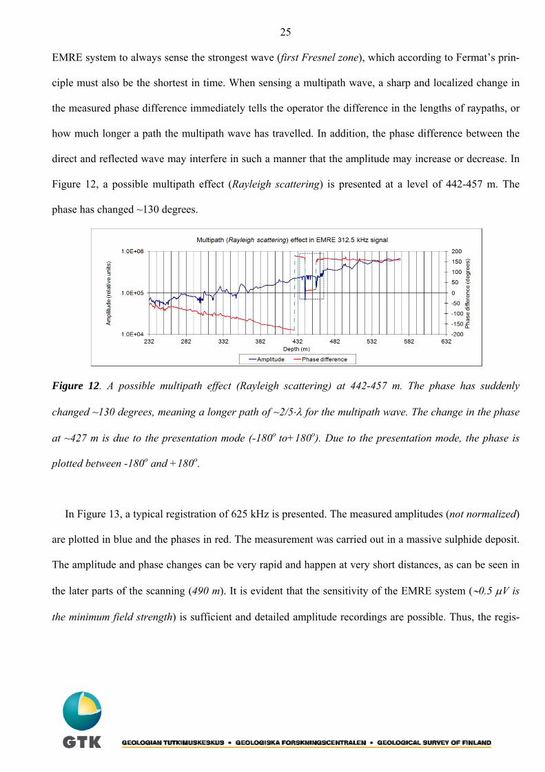
Figure 12, a possible multipath effect (Rayleigh scattering) is presented at a level of 442-457 m. The

phase has changed ~130 degrees.

Figure 12. A possible multipath effect (Rayleigh scattering) at 442-457 m. The phase has suddenly

changed ~130 degrees, meaning a longer path of ~2/5⋅λ for the multipath wave. The change in the phase

at ~427 m is due to the presentation mode (-180o to+180o). Due to the presentation mode, the phase is

plotted between -180o and +180o.

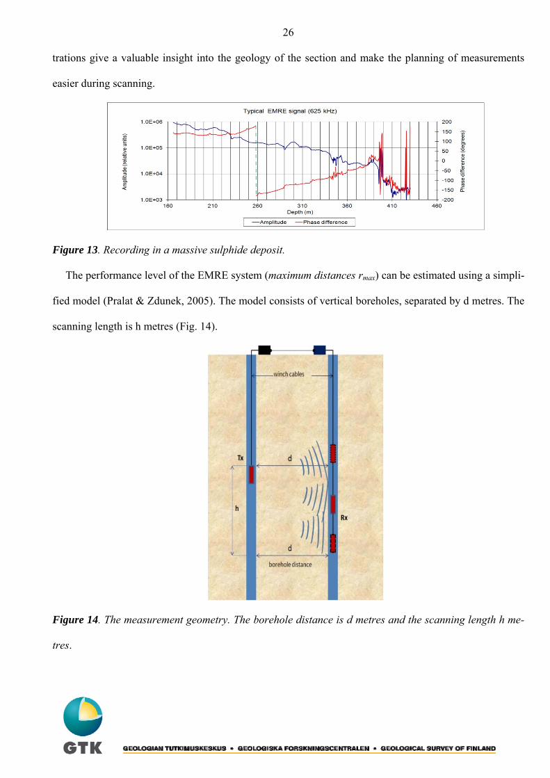
In Figure 13, a typical registration of 625 kHz is presented. The measured amplitudes (not normalized)

are plotted in blue and the phases in red. The measurement was carried out in a massive sulphide deposit.

The amplitude and phase changes can be very rapid and happen at very short distances, as can be seen in

the later parts of the scanning (490 m). It is evident that the sensitivity of the EMRE system (∼0.5 μV is

the minimum field strength) is sufficient and detailed amplitude recordings are possible. Thus, the regis-

26

trations give a valuable insight into the geology of the section and make the planning of measurements

easier during scanning.

Figure 13. Recording in a massive sulphide deposit.

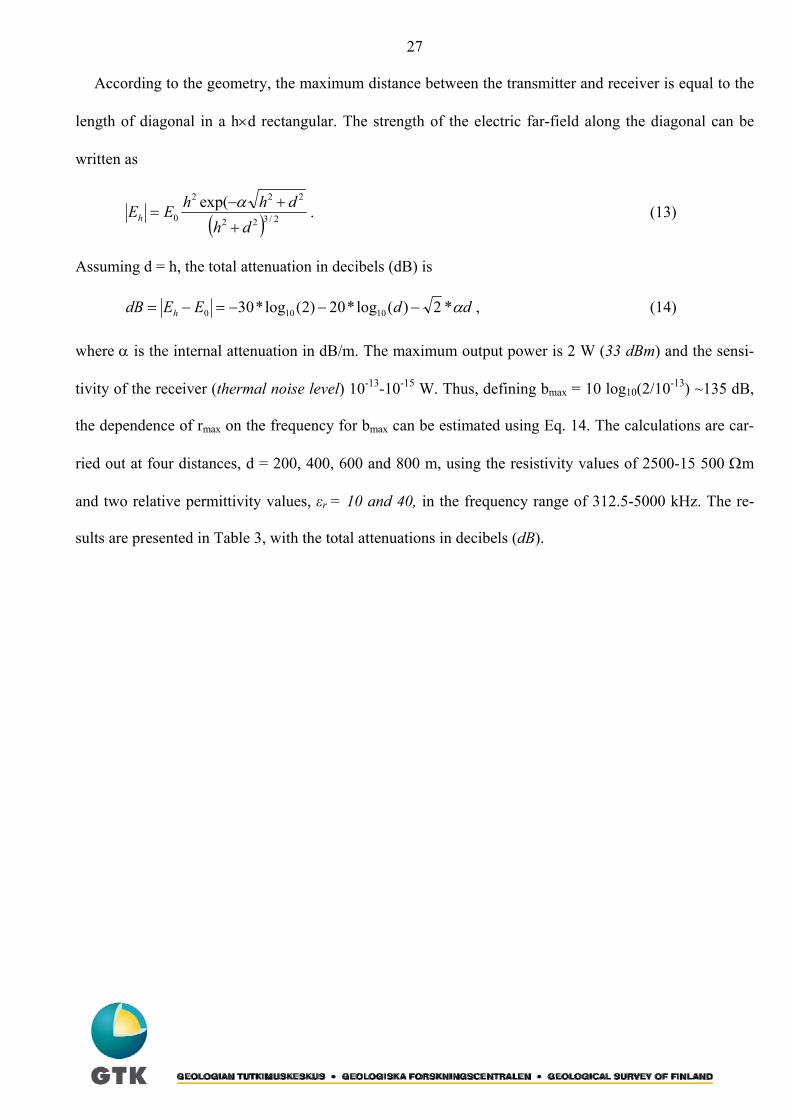
The performance level of the EMRE system (maximum distances rmax) can be estimated using a simpli-

fied model (Pralat & Zdunek, 2005). The model consists of vertical boreholes, separated by d metres. The

scanning length is h metres (Fig. 14).

Figure 14. The measurement geometry. The borehole distance is d metres and the scanning length h me-

tres.

27

According to the geometry, the maximum distance between the transmitter and receiver is equal to the

length of diagonal in a h×d rectangular. The strength of the electric far-field along the diagonal can be

written as

( ) 2/322

222

0exp(

dhdhhEEh

+

+−=

α . (13)

Assuming d = h, the total attenuation in decibels (dB) is

ddEEdB h α*2)(log*20)2(log*30 10100 −−−=−= , (14)

where α is the internal attenuation in dB/m. The maximum output power is 2 W (33 dBm) and the sensi-

tivity of the receiver (thermal noise level) 10-13-10-15 W. Thus, defining bmax = 10 log10(2/10-13) ~135 dB,

the dependence of rmax on the frequency for bmax can be estimated using Eq. 14. The calculations are car-

ried out at four distances, d = 200, 400, 600 and 800 m, using the resistivity values of 2500-15 500 Ωm

and two relative permittivity values, εr = 10 and 40, in the frequency range of 312.5-5000 kHz. The re-

sults are presented in Table 3, with the total attenuations in decibels (dB).

28

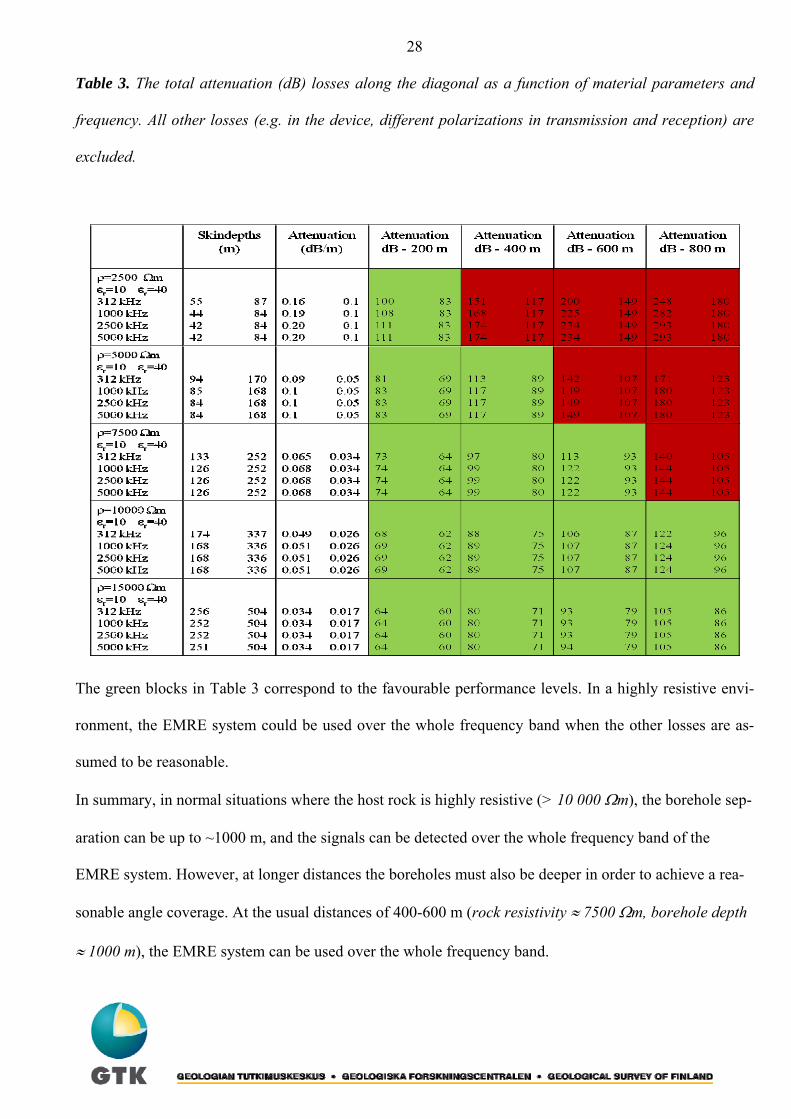
Table 3. The total attenuation (dB) losses along the diagonal as a function of material parameters and

frequency. All other losses (e.g. in the device, different polarizations in transmission and reception) are

excluded.

The green blocks in Table 3 correspond to the favourable performance levels. In a highly resistive envi-

ronment, the EMRE system could be used over the whole frequency band when the other losses are as-

sumed to be reasonable.

In summary, in normal situations where the host rock is highly resistive (> 10 000 Ωm), the borehole sep-

aration can be up to ~1000 m, and the signals can be detected over the whole frequency band of the

EMRE system. However, at longer distances the boreholes must also be deeper in order to achieve a rea-

sonable angle coverage. At the usual distances of 400-600 m (rock resistivity ≈ 7500 Ωm, borehole depth

≈ 1000 m), the EMRE system can be used over the whole frequency band.

29

5 PROCESSING AND INTERPRETATION The problem of forming a cross-sectional image or a tomographic reconstruction arises in a variety of

contexts, including medical tomography (CT) and radiofrequency imaging (RIM) between two deep

boreholes. It is always important to remember that the reconstruction is a registered response of the sub-

surface medium to the existing electromagnetic fields across the used frequency band. Thus, users must

understand the physical meaning of a medium's electrical and magnetic properties, and how these relate to

the attenuation of electromagnetic fields (Korpisalo, 2010b). General purpose methods consists of real

optimization methods where the ultimate goal is to find x that minimizes a cost functional of the form ⎜⎜y-

Ax⎜⎜, where y is a random vector of measurements, x is a vector representing the unknown quantity to be

reconstructed and A is the system matrix. However, in geotomography, many algorithms have been pro-

posed that are not based on the minimizing of any cost functional, and which are formulated as find x

such that y = Ax. These methods are known as special purpose methods. The algebraic reconstruction

technique (ART) (Kak & Slaney, 1999) and the simultaneous iterative reconstruction technique (SIRT)

(Jackson & Tweeton, 1996) are special algorithms. SIRT and ART are traditional methods that are com-

monly used even today. ImageWin (Fullagar, 2004) is a commercial software program for image recon-

struction. In addition to the two algebraic reconstruction methods, the iterative least square method

(LSQR) and the iterative conjugated gradient method (CGLS) are included. If the electrical contrasts are

moderate, the results from the above-mentioned methods are often very good and sufficient. New algo-

rithms, that are also effective with limited angle data (data coverage < 180 degrees), are available in den-

tistry. They could perhaps also be used in solving complicated geotomographic problems, resulting in

more reliable reconstructions of sections.

The data processing is carried out in two stages. In the first stage (editing stage), the raw data are

smoothed and sampled. The signals are cleaned to remove the noisy sections, possible multipath effects

defined by the short and sharp phase changes (Fig. 12) and spurious values (outliers) by rejection and av-

30

erage filtering. Before removing a distinct feature from one frequency, a careful comparison with all fre-

quencies must be performed, and if the feature is missing from the other frequencies, it may be removed.

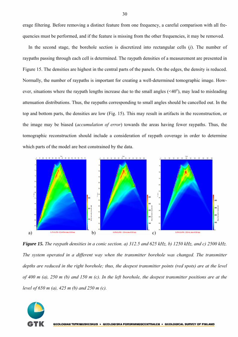
In the second stage, the borehole section is discretized into rectangular cells (j). The number of

raypaths passing through each cell is determined. The raypath densities of a measurement are presented in

Figure 15. The densities are highest in the central parts of the panels. On the edges, the density is reduced.

Normally, the number of raypaths is important for creating a well-determined tomographic image. How-

ever, situations where the raypath lengths increase due to the small angles (<40o), may lead to misleading

attenuation distributions. Thus, the raypaths corresponding to small angles should be cancelled out. In the

top and bottom parts, the densities are low (Fig. 15). This may result in artifacts in the reconstruction, or

the image may be biased (accumulation of error) towards the areas having fewer raypaths. Thus, the

tomographic reconstruction should include a consideration of raypath coverage in order to determine

which parts of the model are best constrained by the data.

a) b) c)

Figure 15. The raypath densities in a conic section. a) 312.5 and 625 kHz, b) 1250 kHz, and c) 2500 kHz.

The system operated in a different way when the transmitter borehole was changed. The transmitter

depths are reduced in the right borehole; thus, the deepest transmitter points (red spots) are at the level

of 400 m (a), 250 m (b) and 150 m (c). In the left borehole, the deepest transmitter positions are at the

level of 650 m (a), 425 m (b) and 250 m (c).

31

In figure 15, the highest densities are displayed in red. This results in a better and more reliable recon-

struction in these regions.

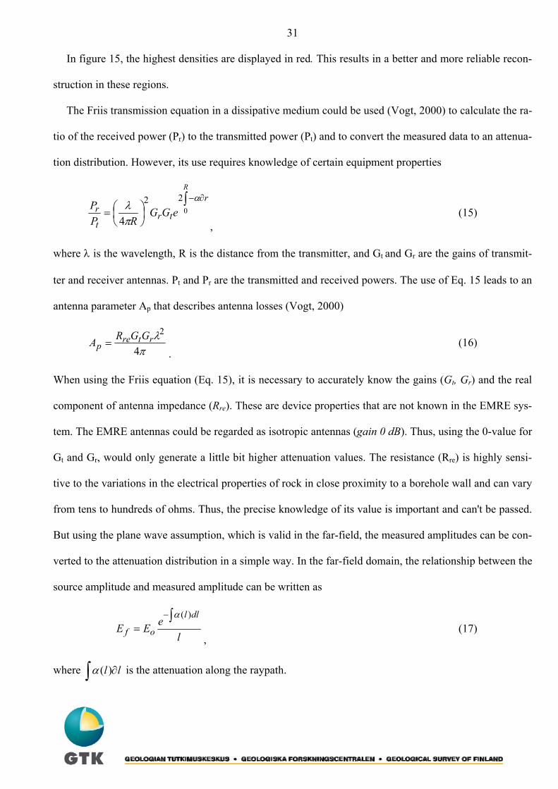
The Friis transmission equation in a dissipative medium could be used (Vogt, 2000) to calculate the ra-

tio of the received power (Pr) to the transmitted power (Pt) and to convert the measured data to an attenua-

tion distribution. However, its use requires knowledge of certain equipment properties

∫ ∂−R

r22 α

⎟⎠⎞

⎜⎝⎛= tr

t

r eGGRP

P 04πλ

, (15)

where λ is the wavelength, R is the distance from the transmitter, and Gt and Gr are the gains of transmit-

ter and receiver antennas. Pt and Pr are the transmitted and received powers. The use of Eq. 15 leads to an

antenna parameter Ap that describes antenna losses (Vogt, 2000)

π

λ4

2rtre

pGGRA =

. (16)

When using the Friis equation (Eq. 15), it is necessary to accurately know the gains (Gt, Gr) and the real

component of antenna impedance (Rre). These are device properties that are not known in the EMRE sys-

tem. The EMRE antennas could be regarded as isotropic antennas (gain 0 dB). Thus, using the 0-value for

Gt and Gr, would only generate a little bit higher attenuation values. The resistance (Rre) is highly sensi-

tive to the variations in the electrical properties of rock in close proximity to a borehole wall and can vary

from tens to hundreds of ohms. Thus, the precise knowledge of its value is important and can't be passed.

But using the plane wave assumption, which is valid in the far-field, the measured amplitudes can be con-

verted to the attenuation distribution in a simple way. In the far-field domain, the relationship between the

source amplitude and measured amplitude can be written as

leEE

dll

of∫−

=)(α

∫ ∂ll )(α

, (17)

where is the attenuation along the raypath.

32

At first, the measured amplitudes must be corrected for the radiation pattern of the antenna and the geo-

metric spreading. Thus, Eq. 17 becomes (Holliger at al., 2001, Holliger & Bergman, 2002)

∫

ΘΓΘΓ=

∫−

dleEE rrtt

dllo

f)()(

)(α

,

(18)

where the denominator contains or the geometric spreading factor, is a correction function of

the transmitter antenna and is a correction function of the receiver antenna. The angles and

are defined in Figure 1. The functions and can be approximated by sinusoidal functions (Zhou and

Fullagar, 2001), in the discrete form. Thus, Eq. 18 along raypath i (j is the cell number) is written as

∫ dl/1 tΓ

rΓ tΘ rΘ

tΓ rΓ

∑ΘΘ

=

∑ −

jij

rt

l

oE l

eE jijj

i

)sin()sin(α

.

(19)

Taking the natural logarithm of Eq. 19 and changing to the common logarithms (decibel units) and rear-

ranging the terms, a reduced equation can be written as

yar

EEr ort −=⎥⎦

⎤⎢⎣⎡ ΘΘ

++−==sinsin

log20)(log20)(log20155.0 1001010ατ , (20)

where the factor 0.155 comes from the logarithm conversion (natural to common) and is equal to

)(log201

10 e. E0 is the unknown source strength that can be estimated by a linear regression of reduced

amplitudes in a homogeneous media. There are two possibilities to handle estimation of the source

strength in ImageWin. In a homogeneous environment, a global source strength can be used for all trans-

mitter positions. In situations where close proximity to a borehole wall changes from one transmitter posi-

tion to another resulting in large variations in the antenna impedance, local source strengths can be used.

Because the antenna impedance is sensitive to the electrical properties of the material near the borehole,

the radiated power is also very different from one transmitter position to another (Korpisalo, 2010a). The

33

first and second term can be combined as , which represents the total intrinsic attenua-

tion (amplitude drop due absorption). The third term includes the angular correction and geometric terms.

The data reduction is completed to provide the attenuation distribution (dB/m) by using the above-

mentioned reconstruction methods (ART, SIRT, LSQR, CGLS). The attenuation distribution can be con-

verted to the conductivity distribution (S/m) using an equation by Zhou (1998)

)/(log20 10 oEE−

f*

*25002

2

πασ = , (21)

where α is the attenuation in Nepers/m and f the frequency in kHz. Eq. 21 is a plane wave solution that is

satisfied in the far-field domain.

The final presentation of the reconstruction is performed using the EMRE– toolbox (Korpisalo, 2009).

As a result, the attenuation or conductivity distribution is presented in the 3D -borehole environment.

When several sections are included in the measurement plan, it is possible to also delineate the targets

that may not be situated directly in the cross section but somewhere in the first Fresnel zone (Fig. 11).

34

6 FIELD CASE IN FINLAND Posiva Oy carries out research and development related to spent nuclear fuel in Finland. The work is con-

centrated at Olkiluoto in the municipality of Eurajoki (in western Finland). Underground characterization

premises, known as ONKALO, have been under construction since 2004. In 2009, a special project was

established between Posiva and GTK to determine the capacity and usefulness of RIM in determining the

structural integrity of the rock in the area. This was the second time (Korpisalo & Niemelä, 2010d), that

RIM measurements had been taken in Olkiluoto, because the pioneering work had already been per-

formed in 2005 (Korpisalo et al. 2008; Korpisalo, 2005). The functioning level of the system was incor-

rect due to the lack of a reference signal, thus, only the amplitude detection was possible. Despite, the at-

tenuation distributions were in good agreement with the results from other methods used in the area. The

massive sulphide deposit at Pyhäsalmi (in central Finland) is an ideal test location for the system, where

the resistive host rock is occupied by a massive conductive ore. The test measurements were continued at

Pyhäsalmi in 2008 (Korpisalo, 2010c).

This paper illustrates the results from Olkiluoto in 2009. The borehole section was quite a challenge

for the EMRE system because the geometry was conic (Fig. 20). The mutual orientation of the antennas

was occasionally very disadvantageous and generated problems. On the other hand, the shape of the sec-

tion also made it possible to start the measurements closer to the Earth's surface without one dominant

wavelength rule to avoid the possible reflection from the Earth's surface. Alternatively, the scanning

could be started near the Earth's surface when the transmitter was located deeper. The highest measure-

ment frequency (2500 kHz) was problematic, as no signals were received. The reason lay not only in the

internal attenuation of the material but also in the unfavourable functioning of the transmitter antenna

(Korpisalo, 2010a). The theoretical scattering parameter s11 that defines the relationship between the input

power and the reflected power in the transmitter, was ~-2dB, thus meaning that ~62% of the power was

reflected back to the generator and only ~38% was radiated. In addition, the large polarization losses in

antennas can also have been significant due to the problematic orientation of the boreholes.

35

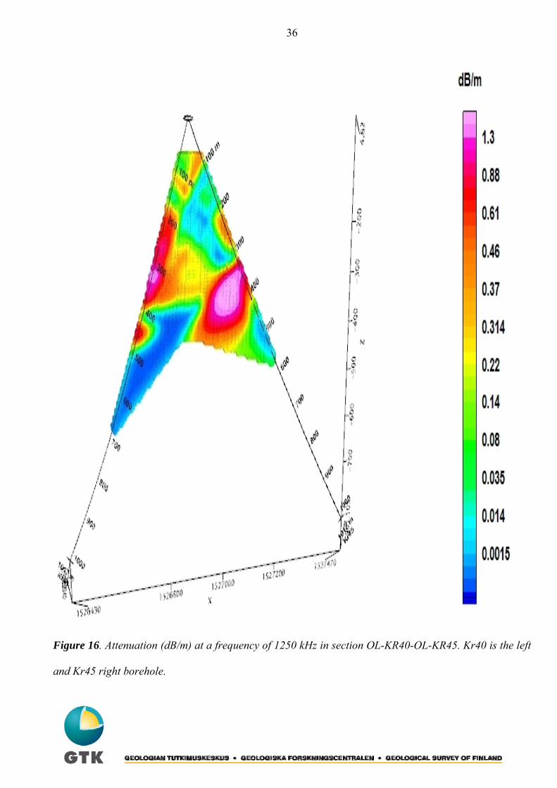
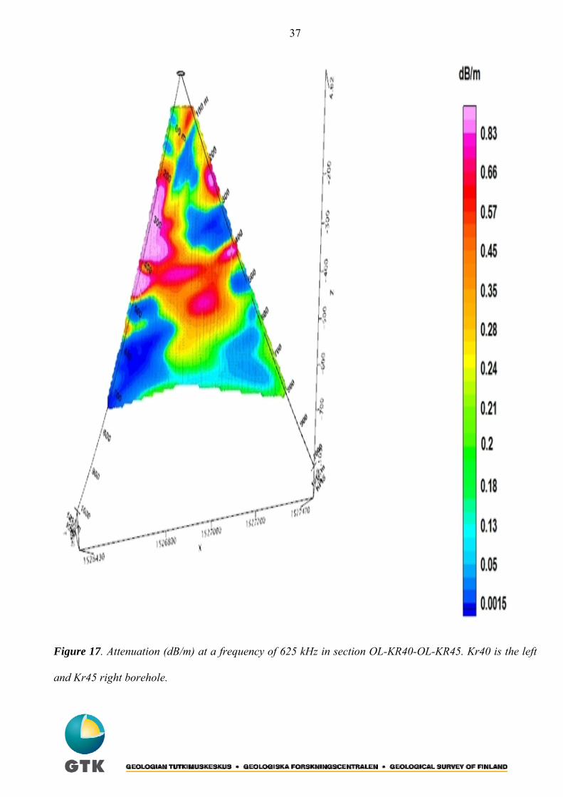
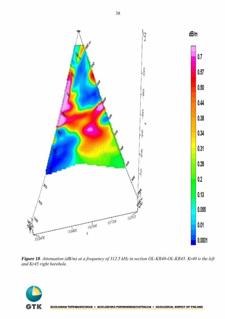
The interpretation was performed by the ImageWin software. The final results with three lower fre-

quencies are presented in Figures 21-23. As a whole, the results coincided very well at the three frequen-

cies. The maximum attenuation rates range from 1.3 dB/m (1250 kHz) to 0.7 dB/m (312.5 kHz). The cor-

responding maximum apparent resistivity value is ~200 Ωm at all frequencies (Eq. 21). The main and

common attenuating zones are clearly visible in all three images. The massive attenuating zone near the

left borehole in the depth range of 200-400 metres dips downwards towards the right borehole and it oc-

curs in all images. In upper part of the right borehole, another common attenuating zone is in the depth

range of 200-300 metres. At 625 kHz, this zone dips downwards towards the left borehole. This feature is

not visible in other images and it may be generated by an object outside the cross section plane and the

object size should be comparable to the wavelength of 625 kHz. There are differences in the distributions,

as would be expected because of the different wavelengths (higher frequencies have shorter wavelengths

and better spatial resolution) and different volumes of the first Fresnel zone. The EMRE system senses

always the strongest signals coming from the first Fresnel and differences are possible in images. The up-

per and lower edges have the greatest potential for errors because of the lower raypath densities, and one

must therefore be careful in drawing final conclusions concerning the edges. For instances, attenuation

seems to be increasing in the head of the cone but careful must be before making any decision about it. It

could be real because all frequencies have the same response. Perhaps, other methods could reveal its fi-

nal nature.

36

Figure 16. Attenuation (dB/m) at a frequency of 1250 kHz in section OL-KR40-OL-KR45. Kr40 is the left

and Kr45 right borehole.

37

Figure 17. Attenuation (dB/m) at a frequency of 625 kHz in section OL-KR40-OL-KR45. Kr40 is the left

and Kr45 right borehole.

38

Figure 18. Attenuation (dB/m) at a frequency of 312.5 kHz in section OL-KR40-OL-KR45. Kr40 is the left and Kr45 right borehole.

39

7 DISCUSSION AND CONCLUSIONS The EMRE system has been taken into productive use at the Geological Survey of Finland (GTK) fol-

lowing a set of test measurements at Olkiluoto (Korpisalo et al. 2008, Korpisalo & Niemelä, 2010e) and

Pyhäsalmi (Korpisalo & Niemelä, 2010d). The system is completed by a modern graphical interface,

EMRE GUI (Korpisalo, 2006), in which the preliminary editing stage is performed, and by a commercial

interpretation program (ImageWin) for the tomographic reconstruction. The final presentation is carried

out with the EMRE module (implemented in Geosoft), in which the attenuation or conductivity distribu-

tion is transferred and displayed in the 3D- borehole environment (Korpisalo, 2009). The three different

cases have proven the potential of the method in exploration geophysics.

The transmitter is a continuous wave (CW) device and all the measurement frequencies are sent simul-

taneously. The nominal output power is 2 W (33dBm). The impedance matching provides the means to

maximize the power transfer or minimize the reflections from the load (antenna). Whenever a transmitter

generator (fixed output impedance) operates with a load, the maximum possible power is delivered to the

load when the impedance of the load is equal to the complex conjugate of the impedance of the source.

For two impedances to be complex conjugates, their resistances must be equal, and their reactances must

be equal in magnitude but of opposite signs. The matching problem has not been solved in our transmitter

due to the broad simultaneous frequency band and highly variable environment properties, which make

the solution impossible. Thus, the total power radiated from the antenna into the rock is reduced. On the

other hand, halving the power only means a decrease of 3 dBm. In the sections (e.g. closely located bore-

holes, saturation), where the response of a frequency or frequencies may be fuzzy, the rejection of a fre-

quency or frequencies from the normal operation can be performed in a jumper board. Thus, the total

power is channelled to the remaining frequencies. The receiver is a superheterodyne-type receiver and it

deviates little from a normal radio receiver. The reception and the double intermediate frequency (IF)

synthesis is performed down in the borehole receiver. The IF frequencies are used as carriers to feed the

measured signals through the winch cable up to the Earth's surface where the final detection is performed.

40

The same mismatching problem concerns the receiver (Korpisalo, 2010c) but it is not as crucial as in the

transmitter.

Normally, the measurements are performed as a fan-beam scanning (ZOM), where the fixed transmit-

ter operates in one borehole and the mobile receiver takes measurements (2 Hz) during movement in the

other borehole. The measurements can be monitored in real time, thus making the control of the scanning

lengths easy and keeping the productivity at a high level. One nominal wavelength rule is used for both

the transmitter and receiver (Fig. 1), or it determines the starting depth levels. The lengths of transmitter

antennas are 20/40 m, thus the transmitter steps of equal lengths can be used because the denser receiver

steps (~0.3 m) ensure dense enough data collection. However, the upper and lower edges of the borehole

section are the most likely artifact sources, so denser transmitter steps may be used in these areas.

The wavelengths from tens to hundreds of metres in the frequency band (312.5-2500 kHz) dictates the

resolution or the smallest features that can be resolved in the bedrock. Higher frequencies (smaller wave-

lengths) mean smaller features can be resolved, but at the same time the ranges are shorter because the

energy transmitted is strongly attenuated. Smaller frequencies (longer wavelengths) have less resolving

power but a greater range. Thus, there is a trade-off between the physical resolution and the range of a

survey. The first field cases have been successful and RIM has risen to the challenge. The method has

been found to have potential in ore exploration among the other geophysical prospecting methods, identi-

fying attenuation (conductivity) variations associated with different geological structures. The smallest

detectable objects need to be 20–30 m thick (very good conductors may be thinner) and continuous in the

lengthwise direction. The thickness corresponds to the wavelength of the highest measurement frequency

(2500 kHz) in a moderate conductive environment.

The interpretation used is based on the far-field solution of electric field. The straight ray assumption

(zero wavelength) is accepted, thus the electromagnetic energy propagates along a ray, and the changes in

the electromagnetic field are generated by the changes in the material properties along the ray. The curved

41

ray paths should generally not be used in amplitude inversion, because the raypath curvature is controlled

by the velocity, not the attenuation. However, in a low-Q (Q << 0.1) regime, the slowness (1/velocity) is

proportional to the attenuation and curved raypaths could be used (Jackson & Tweeton, 1996). However,

when the contrasting electrical properties are moderate, the simple assumption works well. The full wave

field solution of Maxwell’s equations for the electrical dipole field would be useful in the complicated

and inhomogeneous situations, but no software is available that could take into account the complicated

and more realistic characteristics of the environment and the details of borehole antennas and solve the

problem in a reasonable computer time. Practicable solutions to develop the interpretation could be found

in dentistry, where the limited angle problem has been managed to solve in the angle coverage of <180o.

In the EMRE system, the amplitudes and relative phase shifts are measured. As the amplitude is the di-

rectly measurable parameter, it can be used to estimate attenuation, bearing in mind the following. The

far-field condition is assumed where the source and transmitter are separated by several wavelengths.

This may not be completely true in all EMRE surveys, but the approximation makes the interpretation

much easier. The attenuation α is formulated for the Eθ component, having 1/r dependency in the inter-

mediate and far field approximation. In the near-field, the radial Er component with a different attenuation

rate and the static field behaviour having a dependency of r-3 when distances of less than 50–100 m

should be considered. The off-plane conductive targets will also strongly influence the field results. Thus,

the numerical inversion would resolve the case in more detail than the approximate and rapid methods

such as a straight ray method.

In 2009, RIM measurements in borehole section OL-KR40-OL-KR45 were successful. Despite the

challenging measurement geometry, the attenuation distributions with three lower frequencies could be

reconstructed and the results were congruent. At the highest frequency of 2500 kHz, the result was poor

because the received amplitude levels were very low. This could refer possibly to high internal attenua-

tion. However, the frequency suffered mostly from the other reasons (e.g. polarization and reflection

42

losses) and the inherent property of the transmitter. The scattering parameter s11 was at a disturbingly low

level of ~-2dB, and the radiated power was therefore highly reduced (Korpisalo, 2010a). The usefulness

of 1250 kHz was limited to the upper parts of the section, partly for the same reasons as with 2500 kHz.

The lowest transmitter positions were at the level of 250 m in OL-KR45 and 450 m in OL-KR40 (Fig.

16). Both at 625 kHz and 312.5 kHz, the deepest transmitter positions were at the levels of 400 m and 650

m (Figs. 17-18). The longest straight distances between the transmitter and receiver were over 600 m

Thus, the electromagnetic waves could penetrate sufficiently into the rocks in the area, and the measure-

ments could be indicative of the geophysical properties. The bedrock was known to have also sulphide-

rich areas. The resistivity could therefore vary from tens to tens of thousands of ohm metres. It was evi-

dent that RIM could reveal these areas in the bedrock, but the fractured areas were the most interesting

and desirable features. Could the EMRE system rise to the challenge and reveal the small-scaled features?

The existence of sulphide areas made the problem very difficult, because the sulphide content efficiently

masked the influence of fractures. Thus, the cumulative effect of both features could be seen in the tomo-

grams In addition, perhaps the highest frequency with wavelengths of a few tens of metres could had giv-

en a response to the fractures and without any masking.

The reconstructed attenuation images of section OL-KR40-OL-KR45 coincided well with the three

lowest frequencies (Figs. 16-18). The attenuation rates increase with the frequency being highest at the

frequency of 1250 kHz and having a maximum value of 1.3 dB/m (Fig. 16). According to Fig. 8c, the rate

would correspond to a resistivity value of ~200 Ωm. The smallest rates are at the frequency of 312.5 kHz,

ranging from 0.7 dB/m (~200 Ωm) to 0.0015 dB/m (Fig.18). The corresponding middle frequency (625

kHz) values range from 0.83 dB/m (~200 Ωm) to 0.0015 dB/m (Fig. 17). In all images, the common fea-

ture is that the attenuating or conductive material, concentrated at the level of 300 m (OL-KR40), dips

downwards towards OL-KR45. This downwards dipping phenomenon was already evident during the

measurement for the experienced operator. The attenuating concentration at the level of 200- 300 m near

43

borehole OL-KR45 was also well visible at all frequencies. The resolution decreases as a function of de-

creasing frequency, thus the images become more smeared when the frequency is reduced. The smearing

effect in the horizontal direction is always a common feature of the reconstructions, despite the frequency

used, due to the low angle coverage in that direction. On the contrary, the vertical direction doesn't suffer

from smearing.

Inspired by the positive results with RIM, the development of the EMRE system is under consideration,

and an additional high frequency option (5000 kHz) is going to be added to the system. Both the transmit-

ter and receiver will be designed to work more effectively. Weaker signals (~0.1 μV) should be detectable

and a broader dynamic range of 60 dB would increase the usefulness of the device. The angular resolution

of the present device is ~10 degrees, but a resolution of ~2 degrees is possible. These improvements can

be performed, e.g. by improving the frequency synthesis and minimizing phase losses using (TXCO) both

in the transmitter and receiver. In addition, to improve the operation level of the receiver, the present

mixer technique must be modernized and followed by an more effective filter stage. With developments

of this kind, the EMRE system could become a powerful tool in large rock building projects to more pre-

cisely determine the structural integrity of the rock. At present, amplitude data are utilized. However, the

relative phase difference contains information on the relative permittivity. Thus, the development of

phase interpretation is also under consideration.

44

Acknowledgements

I wish to acknowledge RF-specialist Mika Niemelä, who maintained the proper functioning of the EMRE

device. Geophysicists Tapio Ruotoistenmäki and Kimmo Korhonen aided in the preparation of this paper.

45

8 REFERENCES Buselli G., 1980, Electrical geophysics in the USSR, Geophysics, vol. 45, n: 10, 1551-1562.

Daniels D. J., 1996. Surface Penetrating Radar. The Institution of Electrical Engineers. London. United

Kingdom, 1996.

Fullagar P., 2004, ImageWin Geophysical Tomography, Fullagar Geophysics Pty Ltd, February, 2004

Heikkinen E., Korpisalo A., Jokinen T., Popov N., Shuval-Sergeev A., Zhienbaev T., Ahokas T., 2006,

Crosshole radiowave imaging (RIM) at Eurajoki Olkiluoto, Finland, A paper at the International Confer-

ence “Near Surface 2006 in Helsinki”.

Holliger K. , Bergman T., 2002, Numerical modeling of borehole georadar data. Geophysics 67, 1249-

1257.

Holliger K., Musil M., Maurer H. R., 2001, Ray-based amplitude tomography for cross-hole georadar da-

ta: a numerical assessment, J. app. Geoph. 2001, 47, 2856-298

Jackson M. J. & Tweeton D. R., 1996, 3DTOM – Three-dimensional geophysical tomography: USBM

Report of Investigation 9617, 1996.

Kak A. C. & Slaney M., 1998, Principles of Computerized Tomographic Imaging, IEEE Press, 1998.

King R., 1981, Antennas in Materia, Publisher: MIT Press, 1981.

Korpisalo A., 2010a, Borehole antenna considerations in EMRE system: Frequency band 312.5 – 5000

kHz. (Unpublished, part of a PhD thesis).

Korpisalo A., 2010c, “Radio imaging method (RIM) in Finland” (Unpublished, part of a PhD thesis).

Korpisalo A., 2010d, ”RIM measurements in three borehole sections in the Pyhäsalmi area with the

EMRE system”, (Unpublished, part of a PhD thesis).

Korpisalo A. & Niemelä M., 2010e, “Cross-borehole Research with EMRE-System: Radiofrequency

Measurements in Drillhole section OL-KR40-OL-KR45 at Olkiluoto, 2009”, Posiva Working report

2010-24

Korpisalo A., 2009, Radioluotausmittaus (EMRE) –tulosten esittäminen OasisMontaj:ssa, Geological

Survey of Finland, Archive report (in Finnish), Q16.2/2009/14.

Korpisalo A., Jokinen T., Popov N., Shuval-Sergeev A., Zhienbaev T., Heikkinen E., Nummela J., 2008,

“Review of Crosshole Radiowave Imaging (FARA) in Borehole Sections OL-KR4-OL-KR10 and OL-

KR10-OL-KR2 in Olkiluoto”, Posiva Working report 2008-79

46

Korpisalo A., 2007, FARA –laitteen kokoonpano ja käyttö, Geological Survey of Finland, Archive report,

(in Finnish), Q15/2007/13.

Korpisalo A., 2006, Graafinen käyttöliittymä FARA –datan käsittelyyn ja tulkintaan, Geological Survey

of Finland, Archive report, (In Finnish), Q16.2/2006/3.

Korpisalo A., 2005, Radio imaging method with FARA equipment: Crosshole surveys in borehole sec-

tions Kr4-Kr10 and Kr10-Kr2 in Olkiluoto with FARA in 2005, Geological Survey of Finland, Archive

report, Q16.1/2005/1.

Mahrer K. D., 1995, Review of the radio frequency (RIM) method and its utilization in near-surface in-

vestigations, The Leading Edge, April 1995, 249-256.

Orfanidis S.,2008, “Electromagnetic Waves and Antennas”, http://www.ece.rutgers.edu/~orfanidi/ewa/

Pralat A. and Zdunek R., 2005, Electromagnetic Geotomography – Selection of Measuring Frequency,

Sensors Journal, IEEE,Volume 5, Issue 2, April 2005 Page(s): 242 – 250

G V Redko G. V., L V Lebedkin L. V., Shuval-Sergeev A., VIRG-Rudgeofizika, St. Petersburg, Russia, Ste-

vens K., Kazda G, Falconbridge Ltd., Canada, 2000, Borehole electromagnetic geo-physical methods in

ore and coal deposits. A paper at the International Conference “300 years of Russian mine-geological ser-

vice”, Saint-Petersburg (Russia), 2000.

Stevens K, Watts A, Falconbridge Exploration Ltd; Redko G., VIRG-Rudgeofizika, Russian Academy of

Sciences, 1998, In-Mine Applications of the Radiowave Method in the Sudbury Igneous Complex, A pa-

per at the International Conference “Mine Geophysics – 98”, Saint-Petersburg (Russia), 1998.

Seybold J., 2008, Introduction to RF propagation, Wiley, 2008.

Stolarczyk L. G. and Fry R. C., 1986, Radio imaging method (RIM) or diagnostic imaging of anomalous

geologic structures in coal seam waveguides. Transactions of Society for Mining, Metallurgy, and Explo-

ration, Inc., Vol. 288, 1806-1814.

Vogt D,2000, The modelling and design of Radio Tomography antennas, DPhil thesis, unpublished, Uni-

versity of York (United Kingdom), http://www.opengrey.eu/item/display/10068/624370.

Zhang K. and Li D., 2007, Electromagnetic Theory of Microwaves and Optoelectronics, 2007, Springer

Zhou B., Fullagar P. K., 2001, Delineation of sulphide ore zones by borehole radar tomography at

Hellyer mine, Australia J Appl. Geophys. 47, 261-269.

47

Zhou B., Fullagar P. K. and Fallon G. N., 1998, Radio frequency tomography trial at Mt Isa Mine, Explo-

ration geophysics (1998), 29, 675-679.