Computer-aided detection of subtle signs of early breast cancer: Detection of architectural distortion

in mammograms Rangaraj M. Rangayyan

Department of Electrical and Computer Engineering, University of Calgary, Calgary, Alberta, CANADA

2

Breast cancer statistics

Canada: lifetime probability of developing breast cancer is one in 8.8

Canada: lifetime probability of death due to breast cancer is one in 27

Prevalence: 1% of all women living with the disease

Screening mammography has been shown to reduce mortality rates by 30% to 70%

3

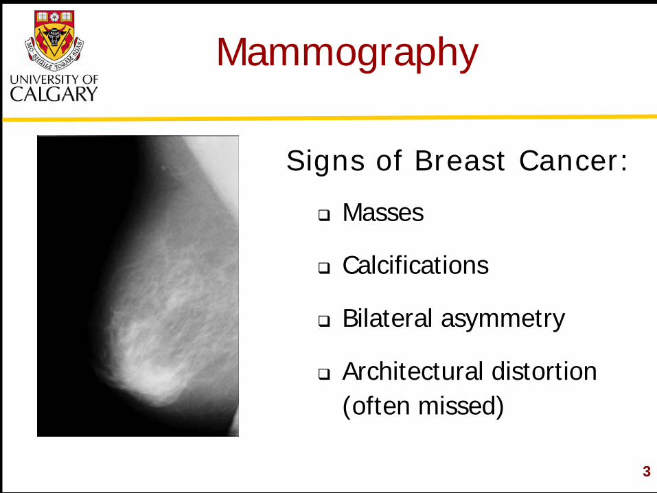
Mammography

Masses

Calcifications

Bilateral asymmetry

Architectural distortion (often missed)

Signs of Breast Cancer:

4

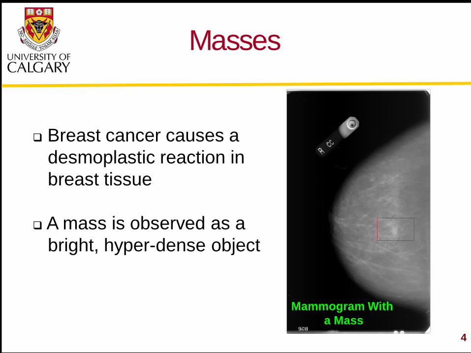
Mammogram With a Mass

Masses

Breast cancer causes a desmoplastic reaction in breast tissue A mass is observed as a bright, hyper-dense object

5

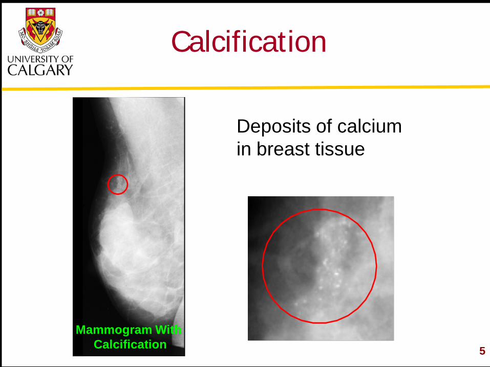
Calcification

Deposits of calcium in breast tissue

Mammogram With Calcification

6

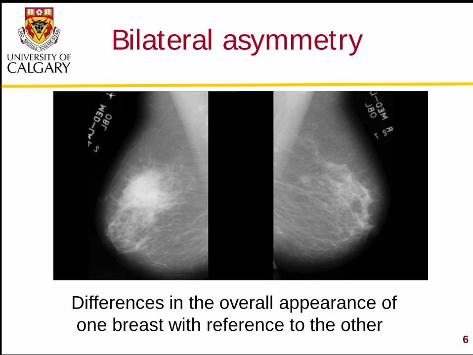
Bilateral asymmetry

Differences in the overall appearance of one breast with reference to the other

7

Computer-aided diagnosis

Increased number of cancers detected1

by 19.5%

Increased early-stage malignancies detected1

from 73% to 78%

Recall rate increased1 from 6.5% to 7.7%

50% of the cases of architectural distortion missed2

1 (Freer and Ulissey, 2001) 2 (Baker et al., 2003)

8

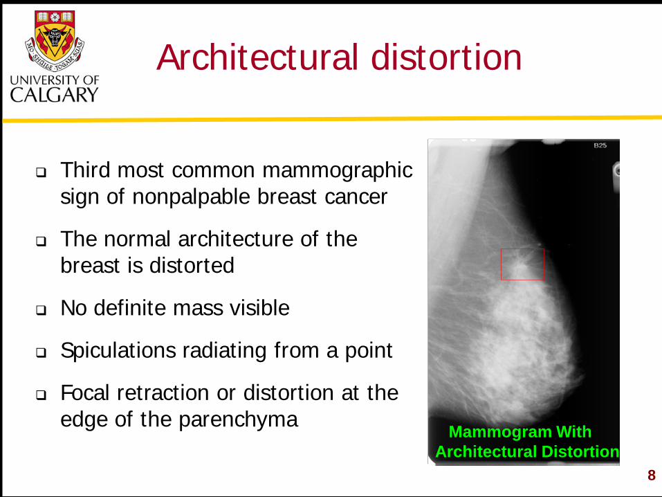
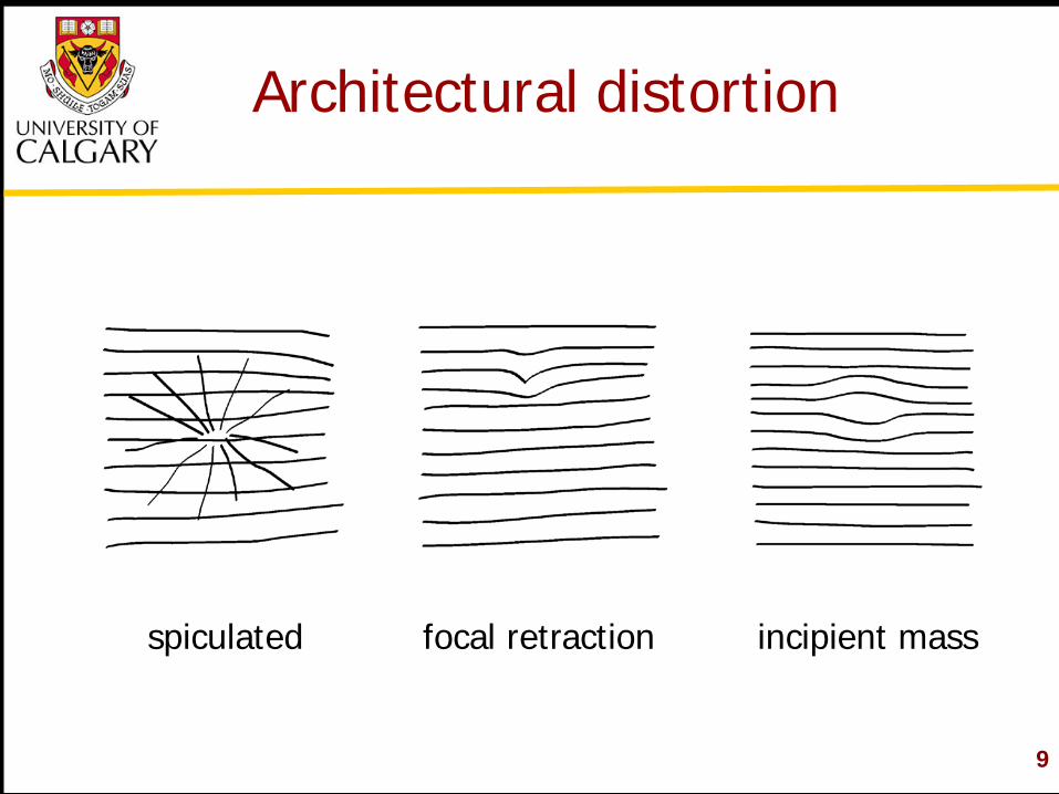
Architectural distortion

Third most common mammographic sign of nonpalpable breast cancer

The normal architecture of the breast is distorted

No definite mass visible

Spiculations radiating from a point

Focal retraction or distortion at the edge of the parenchyma Mammogram With

Architectural Distortion

9

Architectural distortion

spiculated focal retraction incipient mass

10

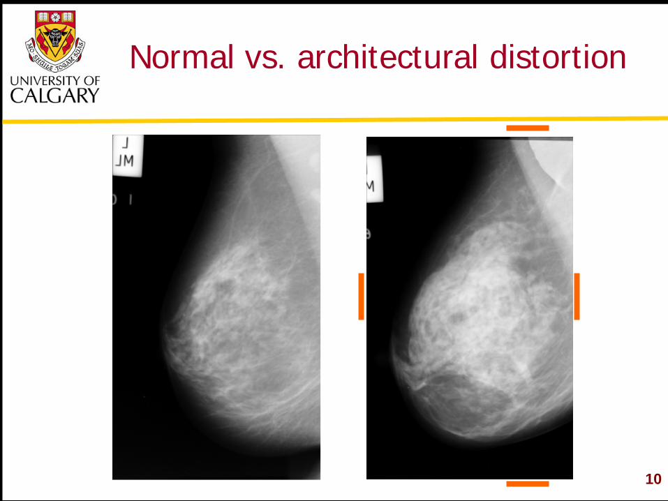
Normal vs. architectural distortion

11

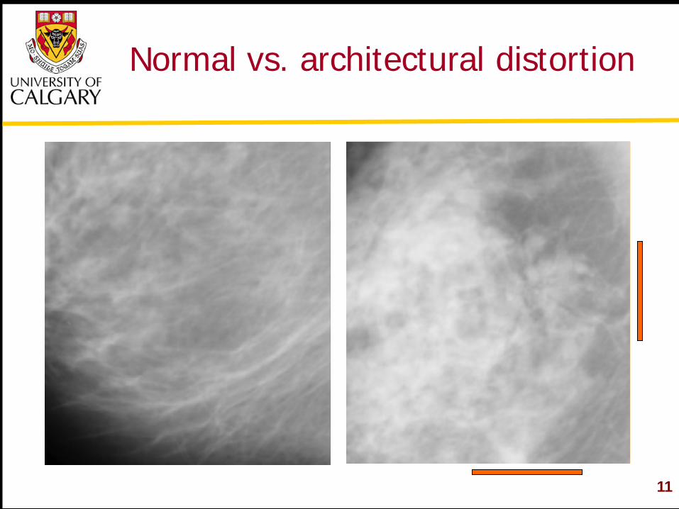
Normal vs. architectural distortion

12

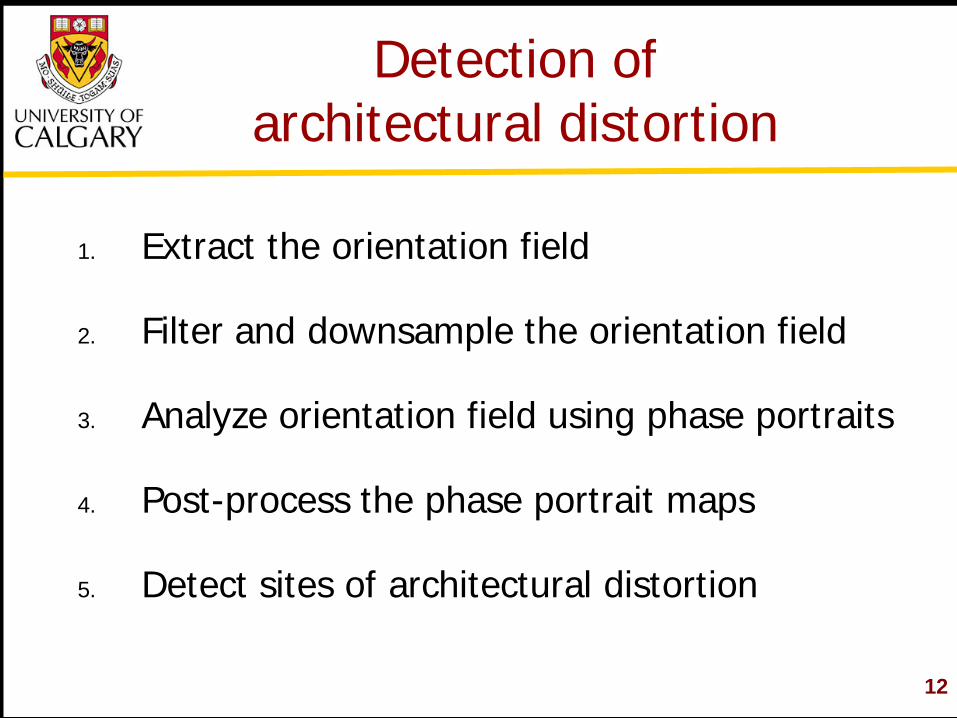
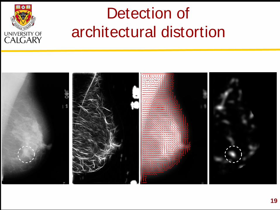
Detection of architectural distortion

1. Extract the orientation field

2. Filter and downsample the orientation field

3. Analyze orientation field using phase portraits

4. Post-process the phase portrait maps

5. Detect sites of architectural distortion

13

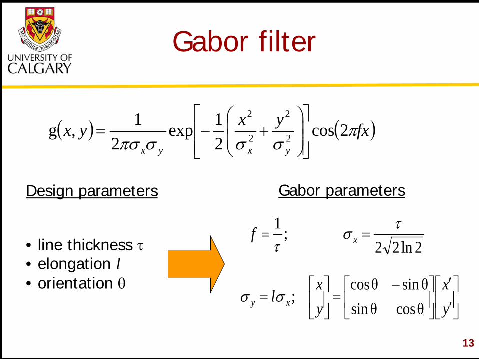
Gabor filter

( ) ( )fxyxyxyxyx

πσσσπσ

2cos21exp

21,g 2

2

2

2

+−=

Design parameters

′′

−=

=

==

yx

yx

l

f

xy

x

θcosθsinθsinθcos

;

2ln22;1

σσ

τστ

Gabor parameters

• line thickness τ • elongation l • orientation θ

14

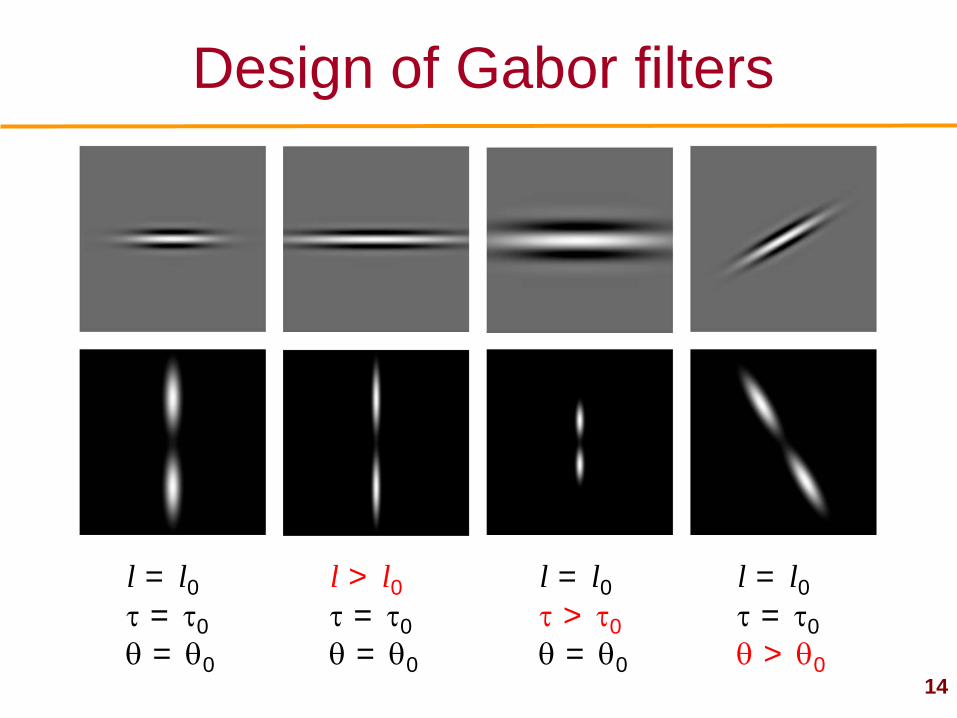
l > l0 τ = τ0 θ = θ0

l = l0 τ > τ0 θ = θ0

l = l0 τ = τ0 θ > θ0

Design of Gabor filters

l = l0 τ = τ0 θ = θ0

15

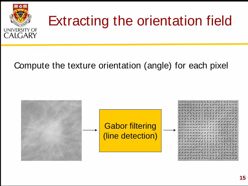
Extracting the orientation field

Compute the texture orientation (angle) for each pixel

Gabor filtering (line detection)

16

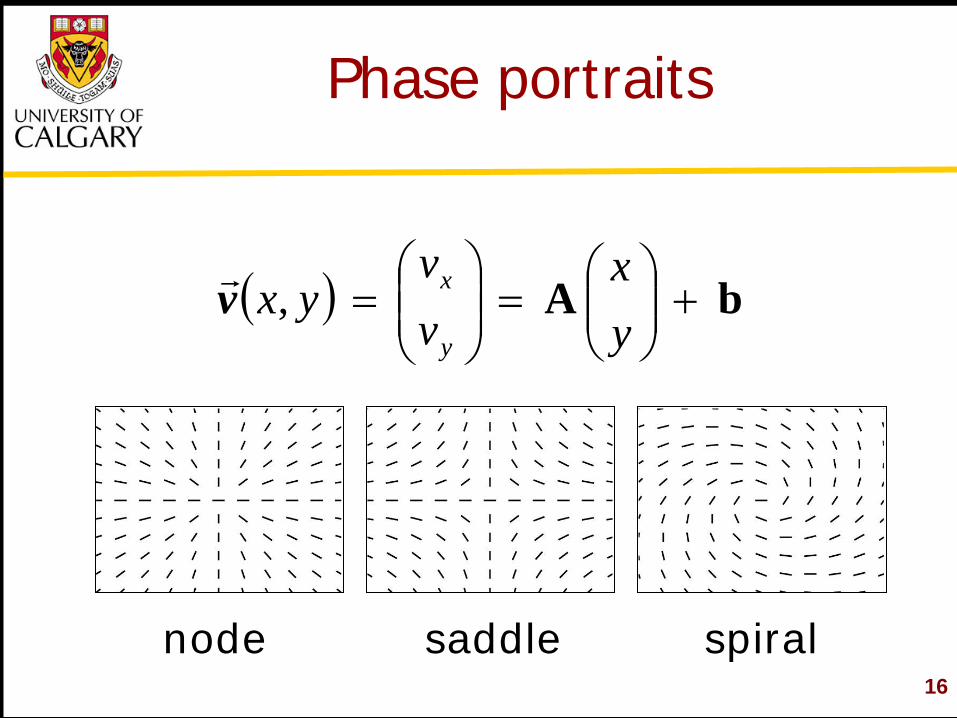
Phase portraits

( ) bA , +

=

=

yx

vv

yxy

xv

node saddle spiral

17

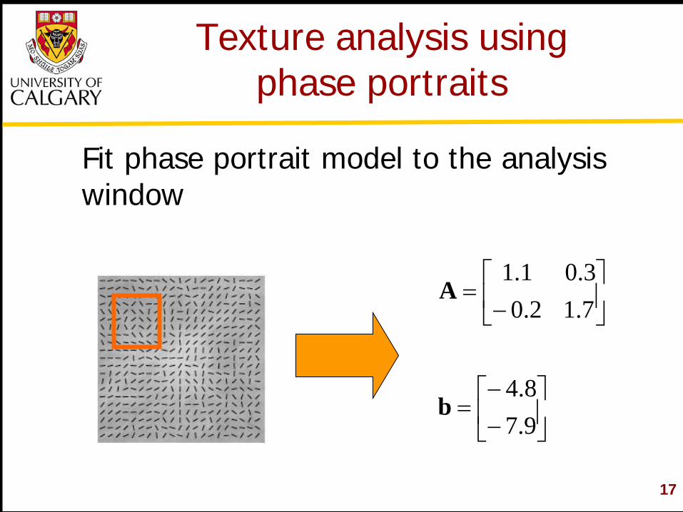
Texture analysis using phase portraits

Fit phase portrait model to the analysis window

−−

=

−

=

9.78.4

7.12.03.01.1

b

A

18

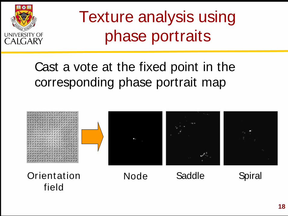
Texture analysis using phase portraits

Cast a vote at the fixed point in the corresponding phase portrait map

Node Saddle Spiral Orientation field

19

Detection of architectural distortion

20

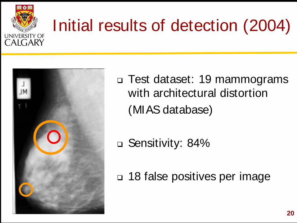
Initial results of detection (2004)

Test dataset: 19 mammograms with architectural distortion

(MIAS database) Sensitivity: 84%

18 false positives per image

21

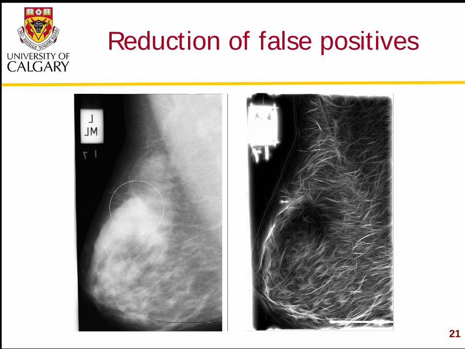
Reduction of false positives

22

Rejection of confounding structures

Confounding structures include Edges of vessels Intersections of vessels Edge of the pectoral muscle Edge of the fibro-glandular disk “Curvilinear Structures”

23

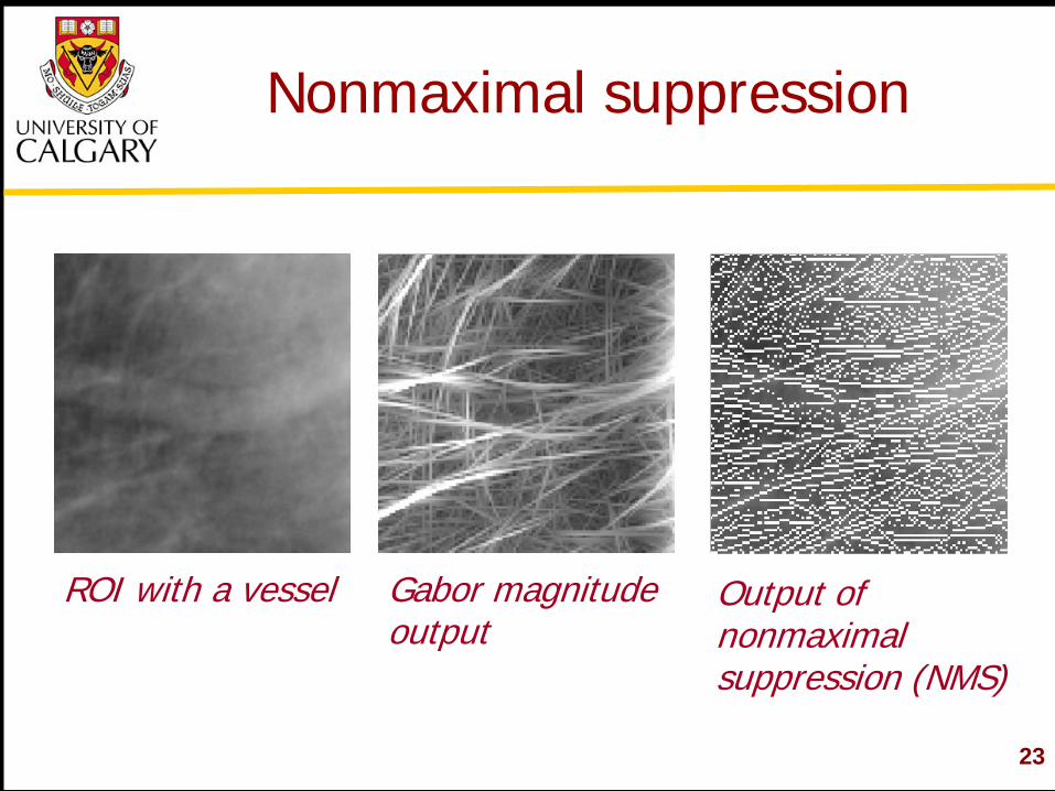
Nonmaximal suppression

ROI with a vessel Output of nonmaximal suppression (NMS)

Gabor magnitude output

24

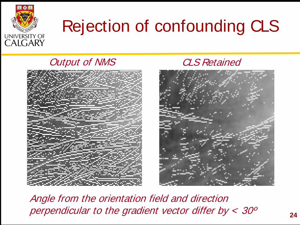
Rejection of confounding CLS

Angle from the orientation field and direction perpendicular to the gradient vector differ by < 30º

Output of NMS CLS Retained

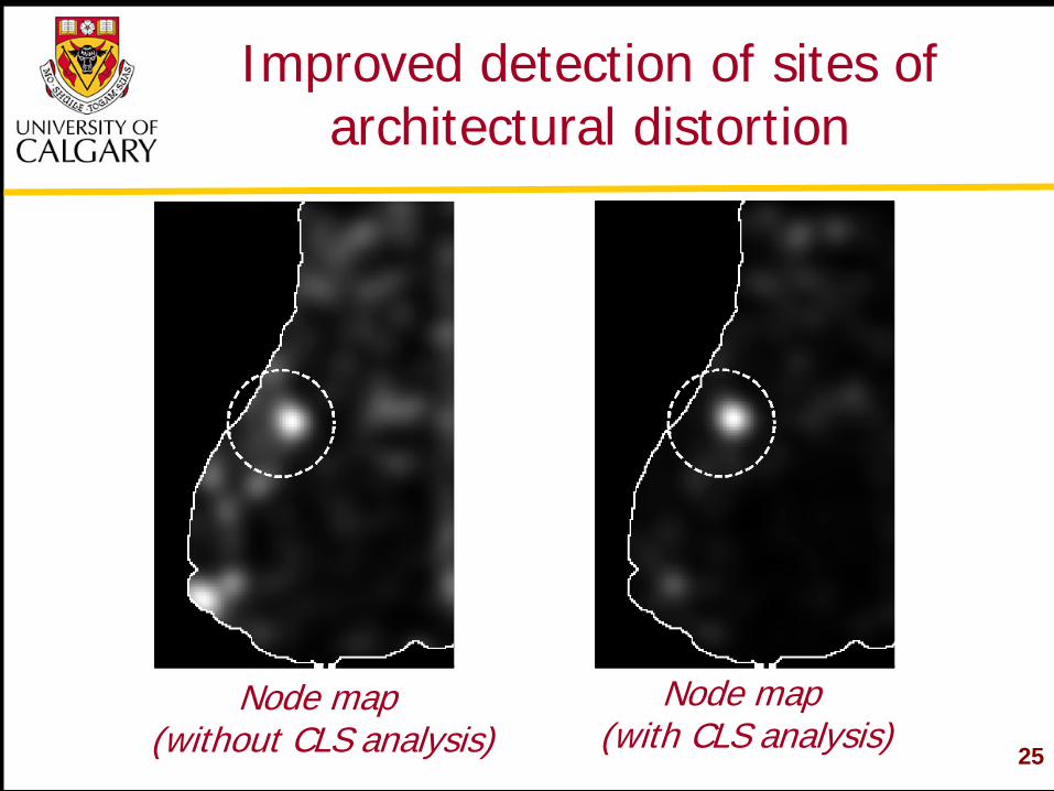
25

Improved detection of sites of architectural distortion

Node map (without CLS analysis)

Node map (with CLS analysis)

26

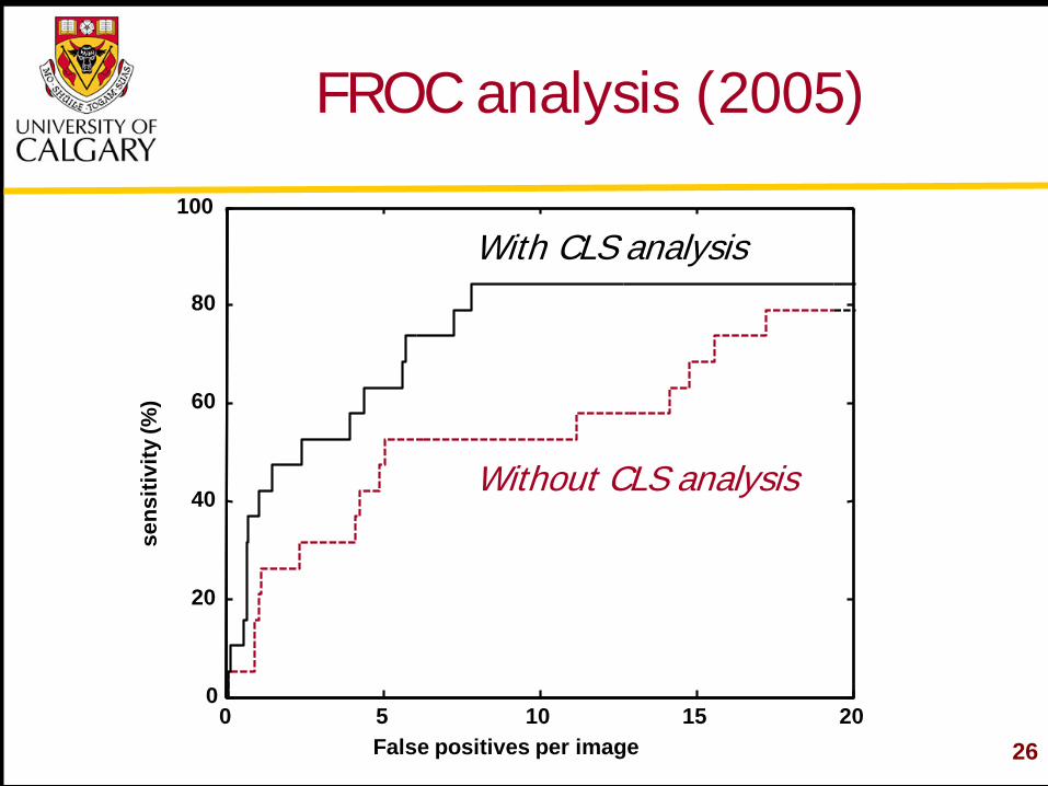
FROC analysis (2005)

0 5 10 15 20 0

20

40

60

80

100

False positives per image

sens

itivi

ty (%

)

With CLS analysis

Without CLS analysis

27

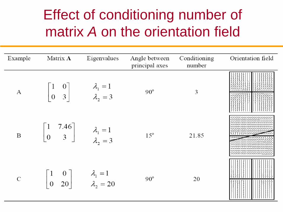
Effect of conditioning number of matrix A on the orientation field

28

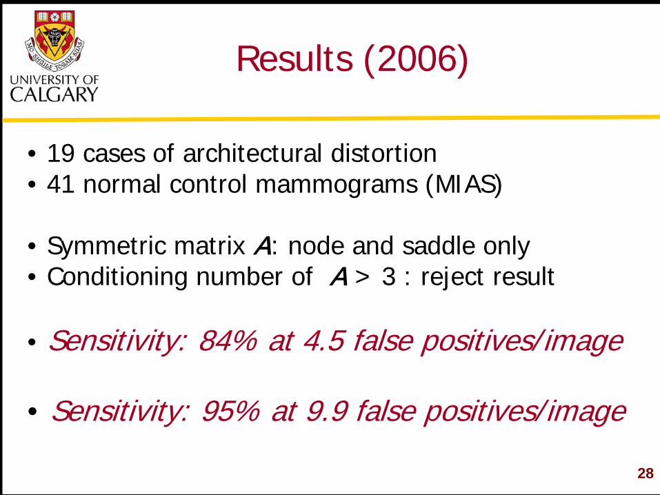
Results (2006)

• 19 cases of architectural distortion • 41 normal control mammograms (MIAS) • Symmetric matrix A: node and saddle only • Conditioning number of A > 3 : reject result

• Sensitivity: 84% at 4.5 false positives/image • Sensitivity: 95% at 9.9 false positives/image

29

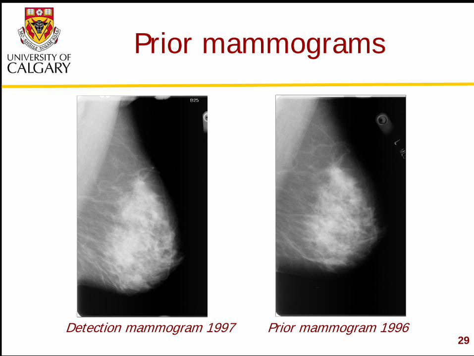
Prior mammograms

Detection mammogram 1997 Prior mammogram 1996

30

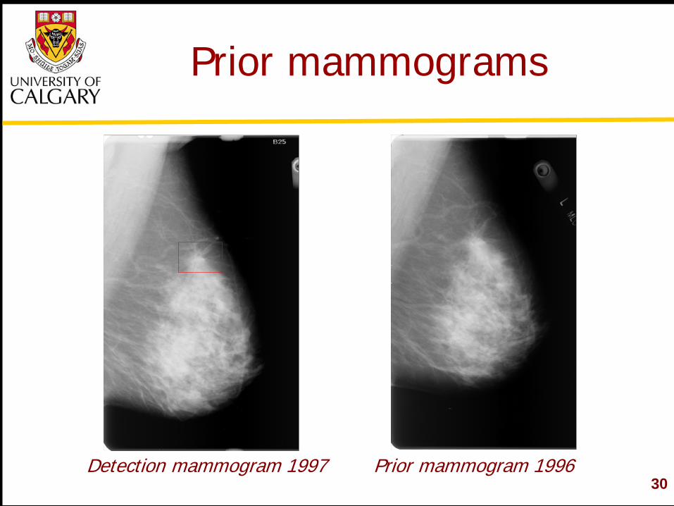
Prior mammograms

Detection mammogram 1997 Prior mammogram 1996

31

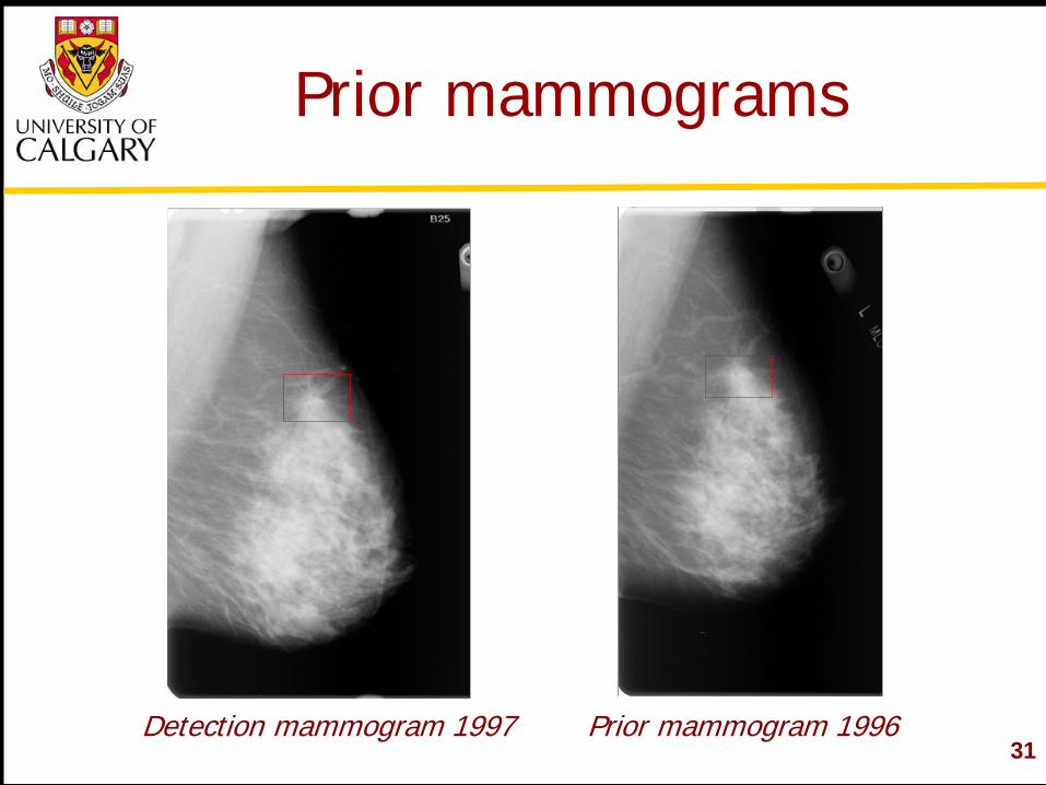
Prior mammograms

Detection mammogram 1997 Prior mammogram 1996

32

Interval cancer

Indicates a case where breast cancer was detected outside the screening program in the interval between scheduled screening sessions.

“Detection Mammograms” were not available.

33

Dataset

106 prior mammographic images of 56 individuals diagnosed with breast cancer (interval-cancer cases).

Time interval between prior and detection (33 cases)- average: 15 months, standard deviation: 7 months, minimum: 1 month, maximum: 24 months.

52 prior mammographic images of 13 normal individuals.

Normal control cases selected represent the penultimate screening visits at the time of preparation of the database.

34

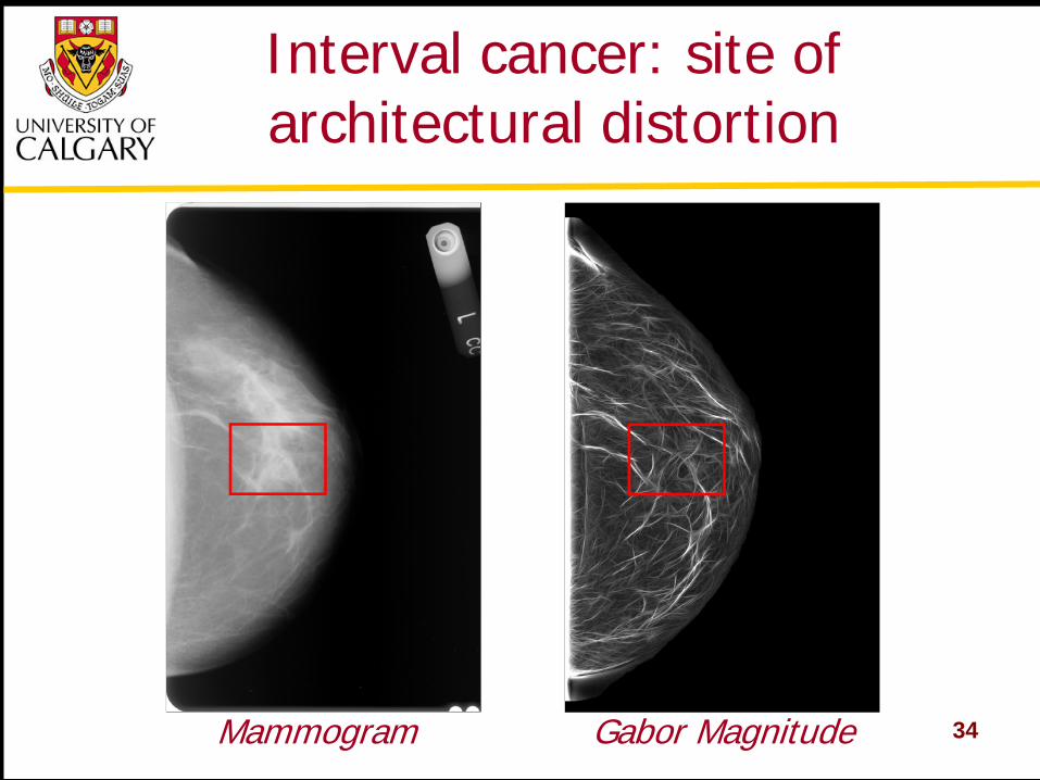
Interval cancer: site of architectural distortion

Mammogram Gabor Magnitude

35

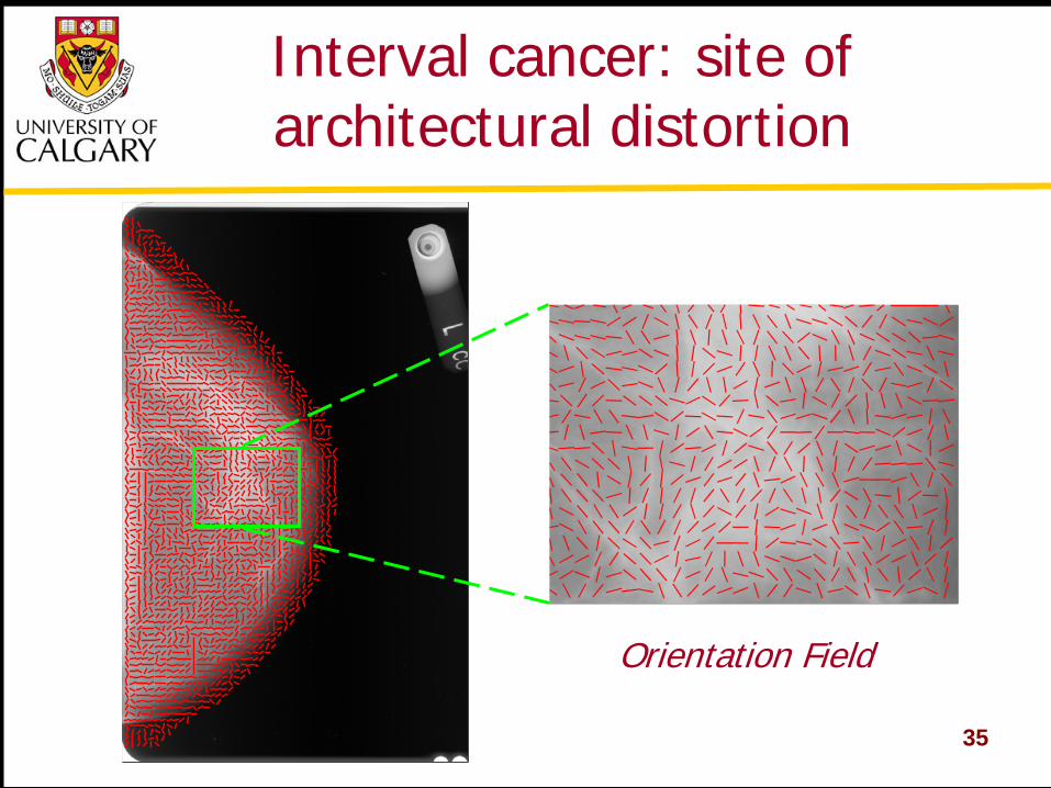
Interval cancer: site of architectural distortion

Orientation Field

36

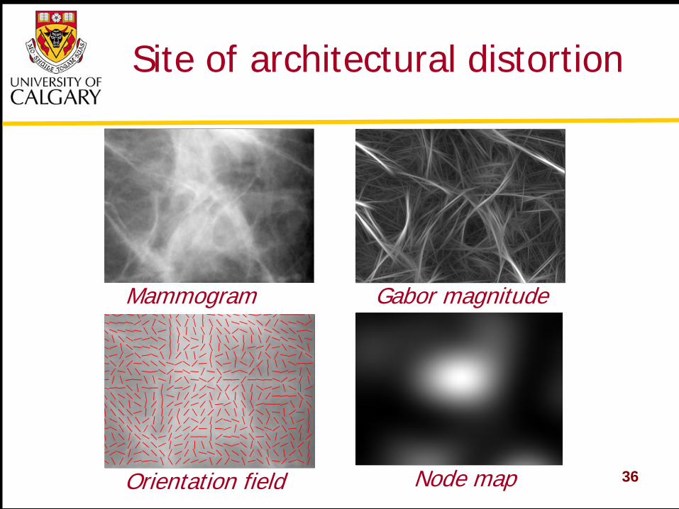
Site of architectural distortion

Mammogram Gabor magnitude

Orientation field Node map

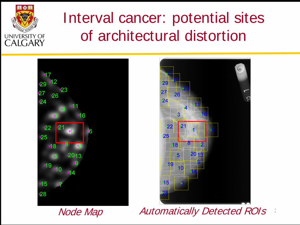
37

Interval cancer: potential sites of architectural distortion

Node Map Automatically Detected ROIs

38

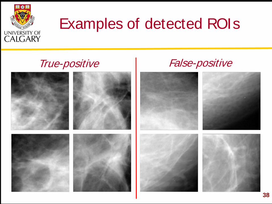
Examples of detected ROIs

True-positive False-positive

39

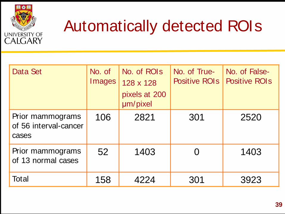
Automatically detected ROIs

Data Set No. of Images

No. of ROIs 128 x 128 pixels at 200 μm/pixel

No. of True- Positive ROIs

No. of False- Positive ROIs

Prior mammograms of 56 interval-cancer cases

106

2821 301 2520

Prior mammograms of 13 normal cases

52

1403 0 1403

Total 158 4224 301 3923

40

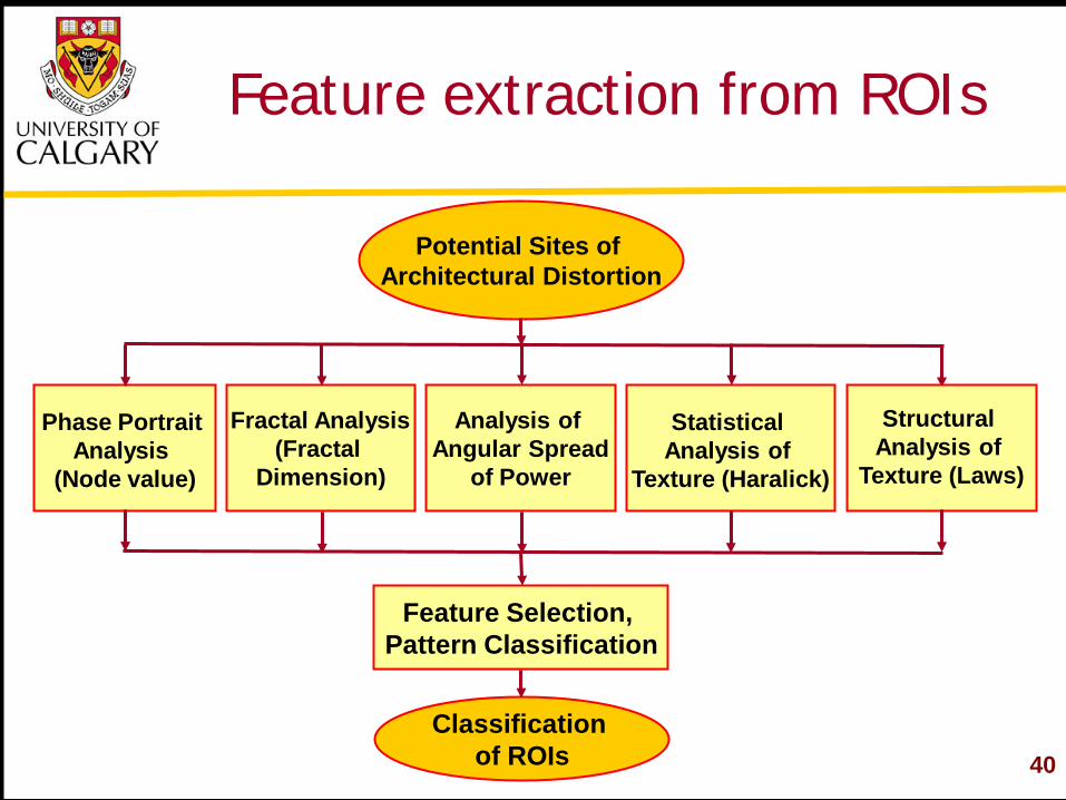
Feature extraction from ROIs

Potential Sites of Architectural Distortion

Feature Selection, Pattern Classification

Classification of ROIs

Phase Portrait

Analysis (Node value)

Fractal Analysis

(Fractal Dimension)

Analysis of

Angular Spread of Power

Statistical

Analysis of Texture (Haralick)

Structural

Analysis of Texture (Laws)

41

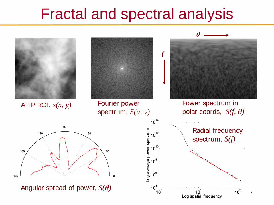
Fractal and spectral analysis

A TP ROI, s(x, y) Fourier power spectrum, S(u, v)

Power spectrum in polar coords, S(f, θ)

θ

f

Angular spread of power, S(θ)

Radial frequency spectrum, S(f)

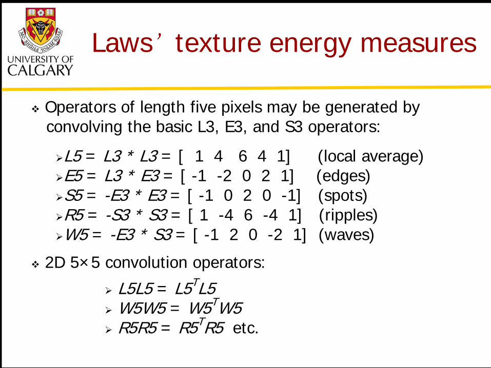
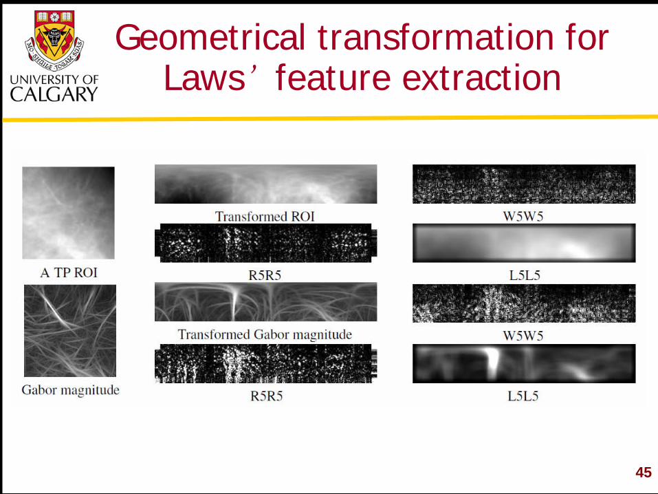
Laws’ texture energy measures

Operators of length five pixels may be generated by convolving the basic L3, E3, and S3 operators:

L5 = L3 * L3 = [ 1 4 6 4 1] (local average) E5 = L3 * E3 = [ -1 -2 0 2 1] (edges) S5 = -E3 * E3 = [ -1 0 2 0 -1] (spots) R5 = -S3 * S3 = [ 1 -4 6 -4 1] (ripples) W5 = -E3 * S3 = [ -1 2 0 -2 1] (waves)

2D 5×5 convolution operators:

L5L5 = L5TL5 W5W5 = W5TW5 R5R5 = R5TR5 etc.

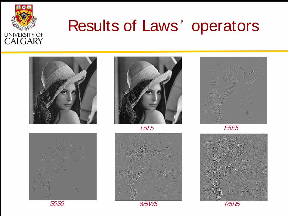
Results of Laws’ operators

L5L5 E5E5

S5S5 W5W5 R5R5

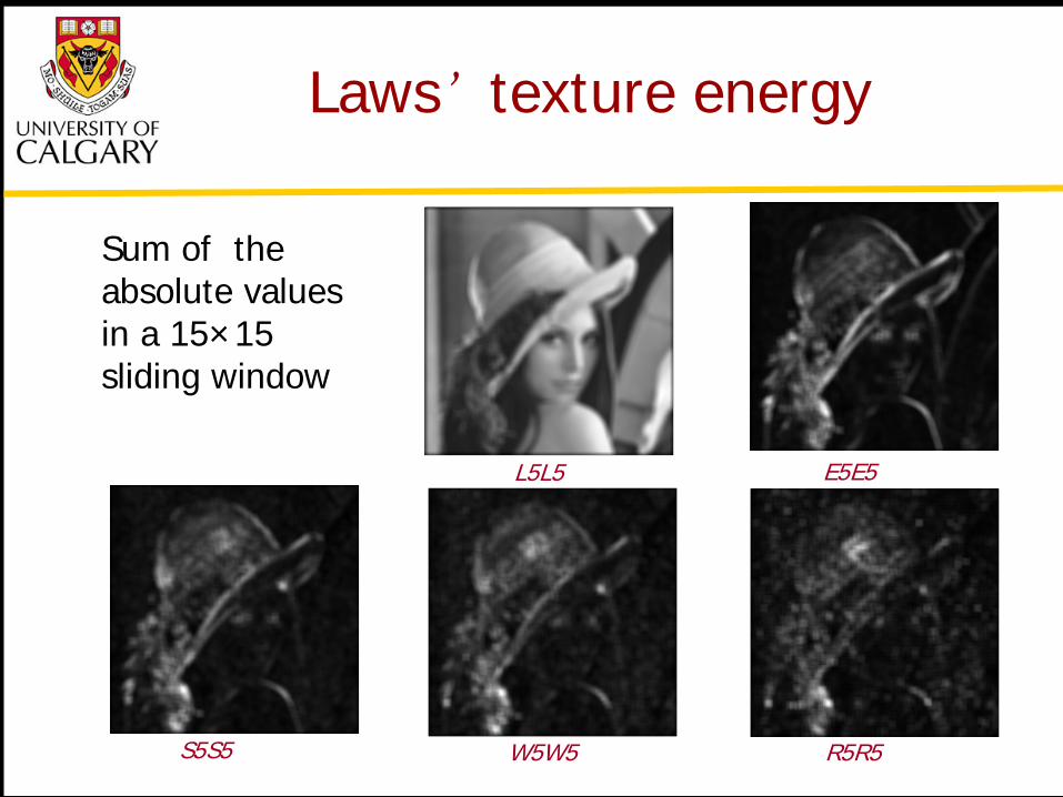
Laws’ texture energy

L5L5 E5E5

S5S5 W5W5 R5R5

Sum of the absolute values in a 15×15 sliding window

45

Geometrical transformation for Laws’ feature extraction

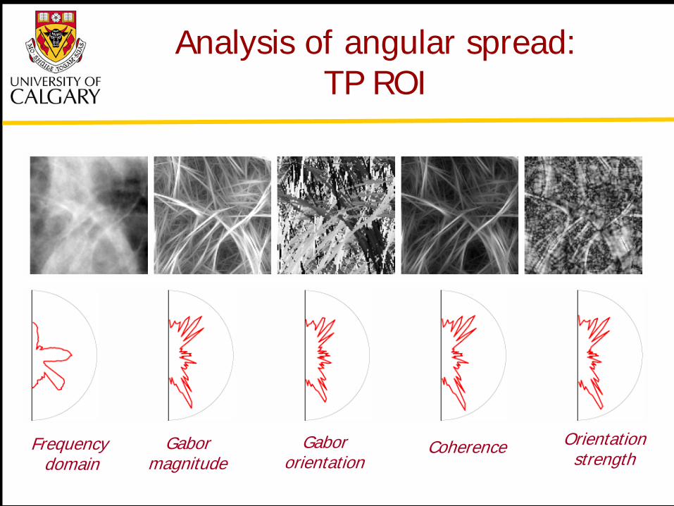
Analysis of angular spread: TP ROI

Gabor magnitude

Gabor orientation

Coherence Orientation strength

Frequency domain

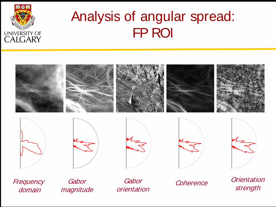
Analysis of angular spread: FP ROI

Gabor magnitude

Gabor orientation

Coherence Orientation strength

Frequency domain

48

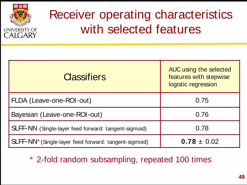
Receiver operating characteristics with selected features

Classifiers AUC using the selected features with stepwise logistic regression

FLDA (Leave-one-ROI-out) 0.75

Bayesian (Leave-one-ROI-out) 0.76

SLFF-NN (Single-layer feed forward: tangent-sigmoid) 0.78

SLFF-NN*(Single-layer feed forward: tangent-sigmoid) 0.78 ± 0.02

* 2-fold random subsampling, repeated 100 times

49

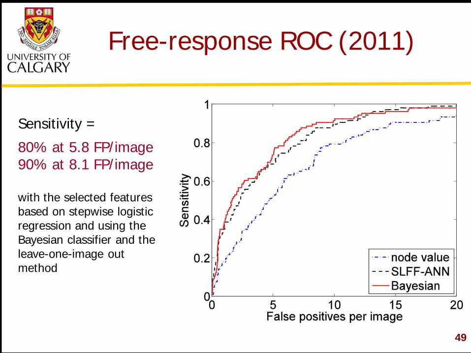
Free-response ROC (2011)

Sensitivity =

80% at 5.8 FP/image 90% at 8.1 FP/image with the selected features based on stepwise logistic regression and using the Bayesian classifier and the leave-one-image out method

50

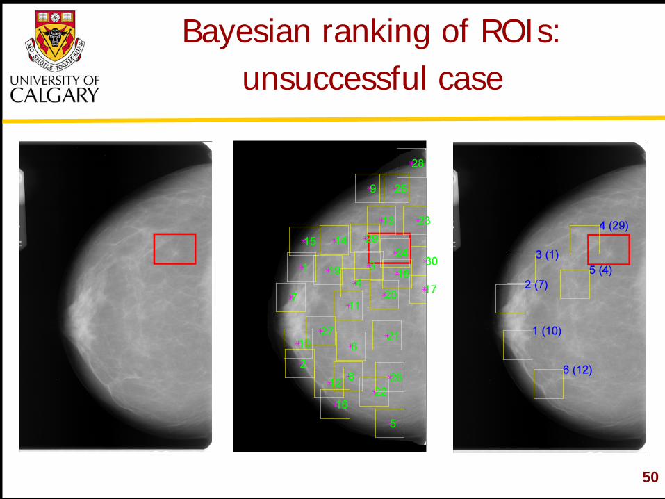
Bayesian ranking of ROIs: unsuccessful case

51

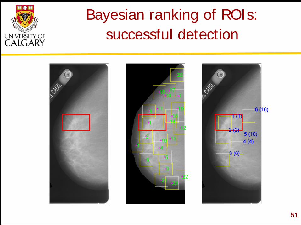
Bayesian ranking of ROIs: successful detection

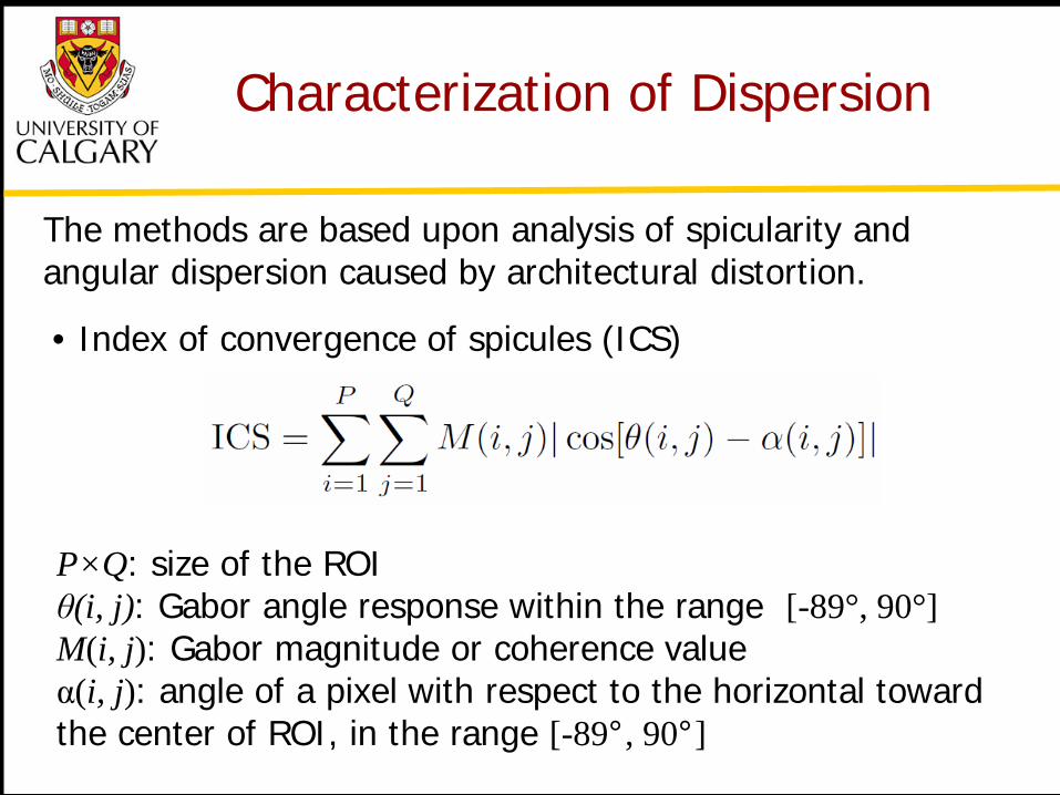
Characterization of Dispersion

The methods are based upon analysis of spicularity and angular dispersion caused by architectural distortion.

• Index of convergence of spicules (ICS)

P×Q: size of the ROI θ(i, j): Gabor angle response within the range [-89°, 90°] M(i, j): Gabor magnitude or coherence value α(i, j): angle of a pixel with respect to the horizontal toward the center of ROI, in the range [-89°, 90°]

Index of Convergence of Spicules

ICS quantifies the degree of alignment of each pixel toward the center of the ROI weighted by the Gabor magnitude or coherence value.

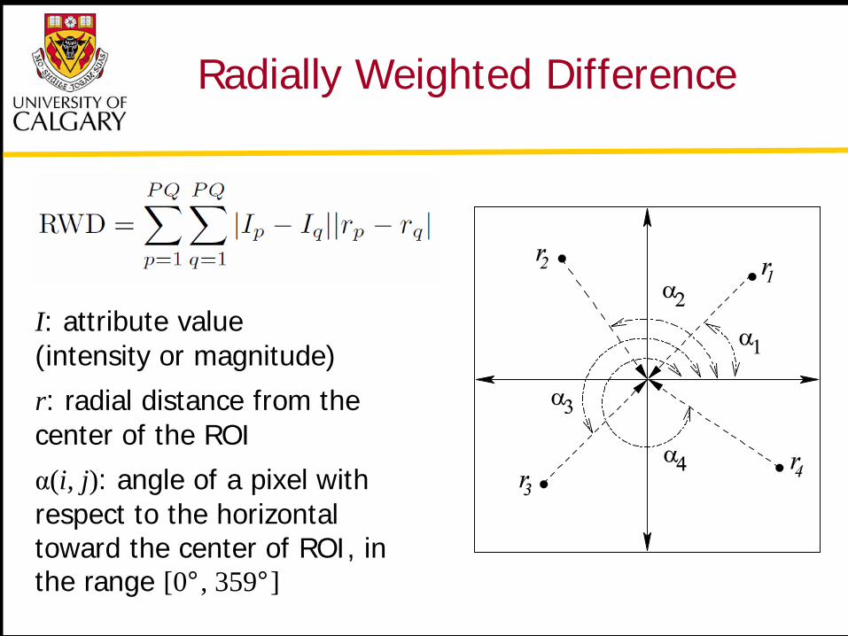
Radially Weighted Difference

I: attribute value (intensity or magnitude)

r: radial distance from the center of the ROI

α(i, j): angle of a pixel with respect to the horizontal toward the center of ROI, in the range [0°, 359°]

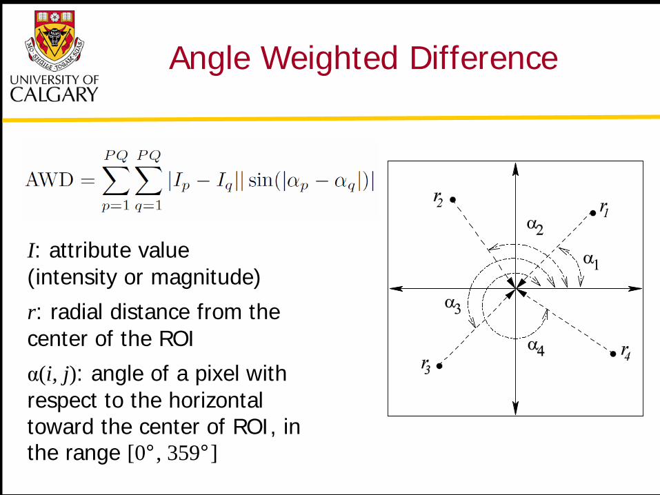
Angle Weighted Difference

I: attribute value (intensity or magnitude)

r: radial distance from the center of the ROI

α(i, j): angle of a pixel with respect to the horizontal toward the center of ROI, in the range [0°, 359°]

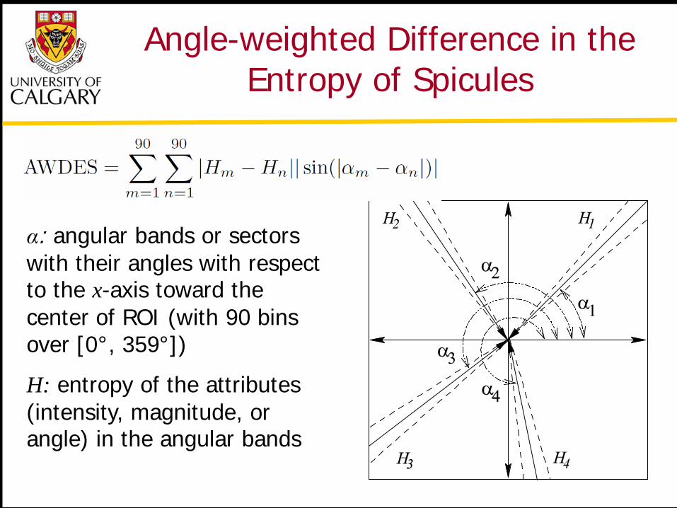
Angle-weighted Difference in the Entropy of Spicules

α: angular bands or sectors with their angles with respect to the x-axis toward the center of ROI (with 90 bins over [0°, 359°])

H: entropy of the attributes (intensity, magnitude, or angle) in the angular bands

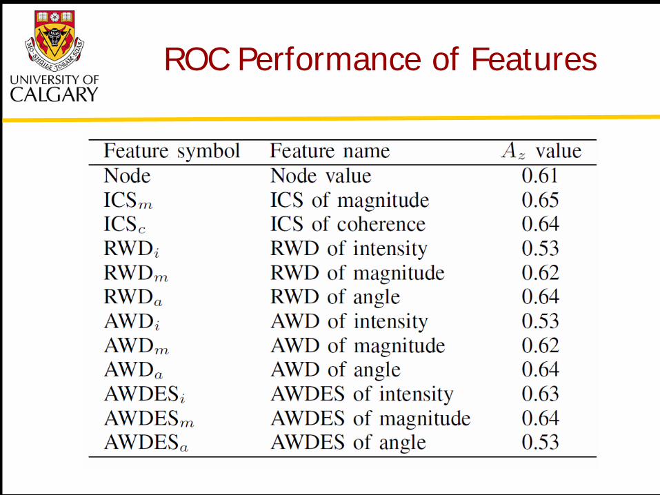
ROC Performance of Features

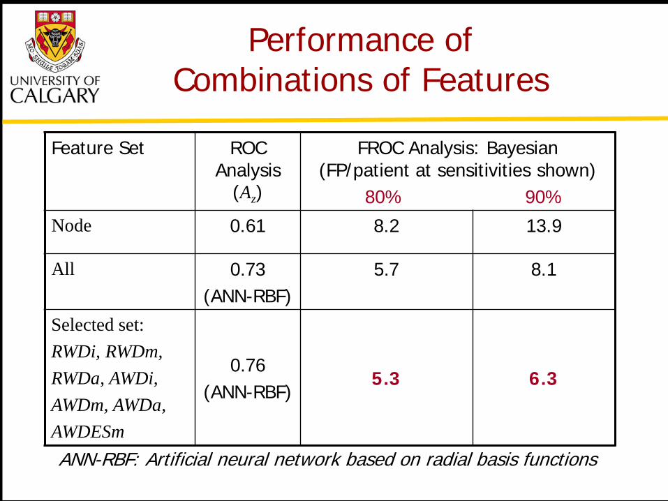
Performance of Combinations of Features

Feature Set ROC Analysis

(Az)

FROC Analysis: Bayesian (FP/patient at sensitivities shown)

80% 90% Node 0.61 8.2 13.9

All 0.73 (ANN-RBF)

5.7 8.1

Selected set: RWDi, RWDm, RWDa, AWDi, AWDm, AWDa, AWDESm

0.76 (ANN-RBF)

5.3 6.3

ANN-RBF: Artificial neural network based on radial basis functions

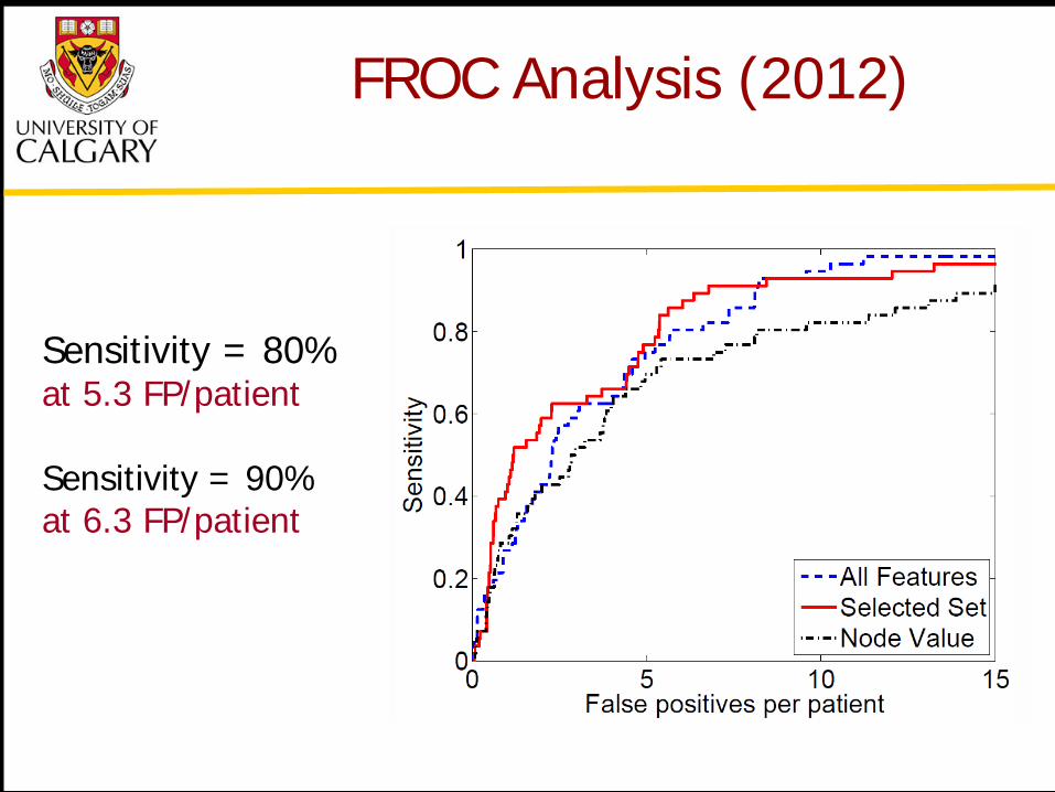
FROC Analysis (2012)

Sensitivity = 80% at 5.3 FP/patient

Sensitivity = 90% at 6.3 FP/patient

Other Approaches to Detect Architectural Distortion

Karssemeijer and te Brake, IEEE TMI 1996: multiscale-based method using the output of three-directional, second-order, Gaussian derivative operators Sampat et al., IEEE SW Symp. Im. An. Int. 2006: linear filtering of the Radon transform of the given image for the enhancement of spicules; the enhanced image was filtered with radial spiculation filters

Matsubara et al., CARS 2003, 2004: detection of architectural distortion near the skin line Nemoto et al., IJCARS 2009: lines corresponding to spiculation of architectural distortion differ in characteristics from lines in the normal mammary gland; modified point convergence index weighted by the likelihood of spiculation calculated to enhance architectural distortion

Other Approaches to Detect Architectural Distortion

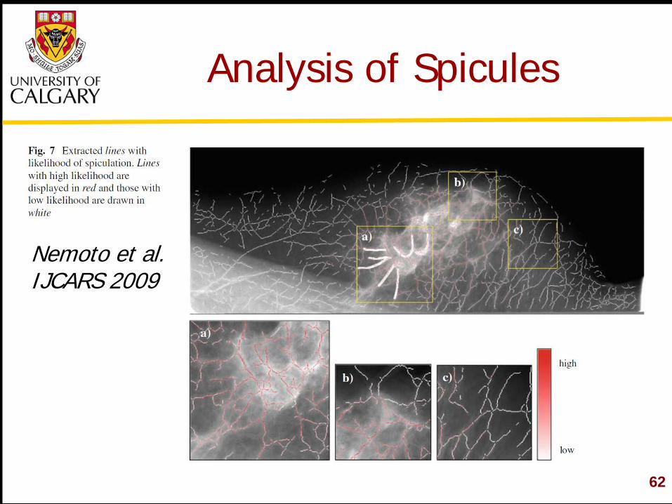
Analysis of Spicules

62

Nemoto et al. IJCARS 2009

Fractal Analysis

Guo et al. IJCARS 2009: fractional Brownian motion model; regions with masses and architectural distortion have lower fractal dimension and higher lacunarity than normal regions Tourassi et al. Phys. Med. Biol. 2006: fractal dimension using power spectral analysis Rangayyan et al. IJCARS 2007: fractal analysis and texture analysis of ROIs detected in prior mammograms of cases of screen-detected cancer 63

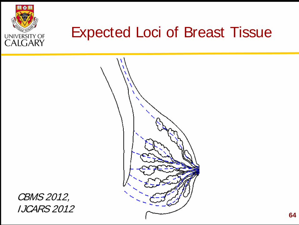
Expected Loci of Breast Tissue

64

CBMS 2012, IJCARS 2012

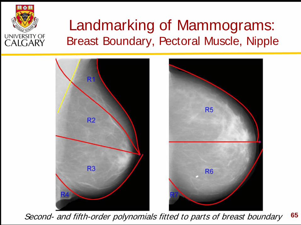
Landmarking of Mammograms: Breast Boundary, Pectoral Muscle, Nipple

Second- and fifth-order polynomials fitted to parts of breast boundary 65

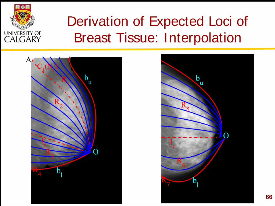
Derivation of Expected Loci of Breast Tissue: Interpolation

66

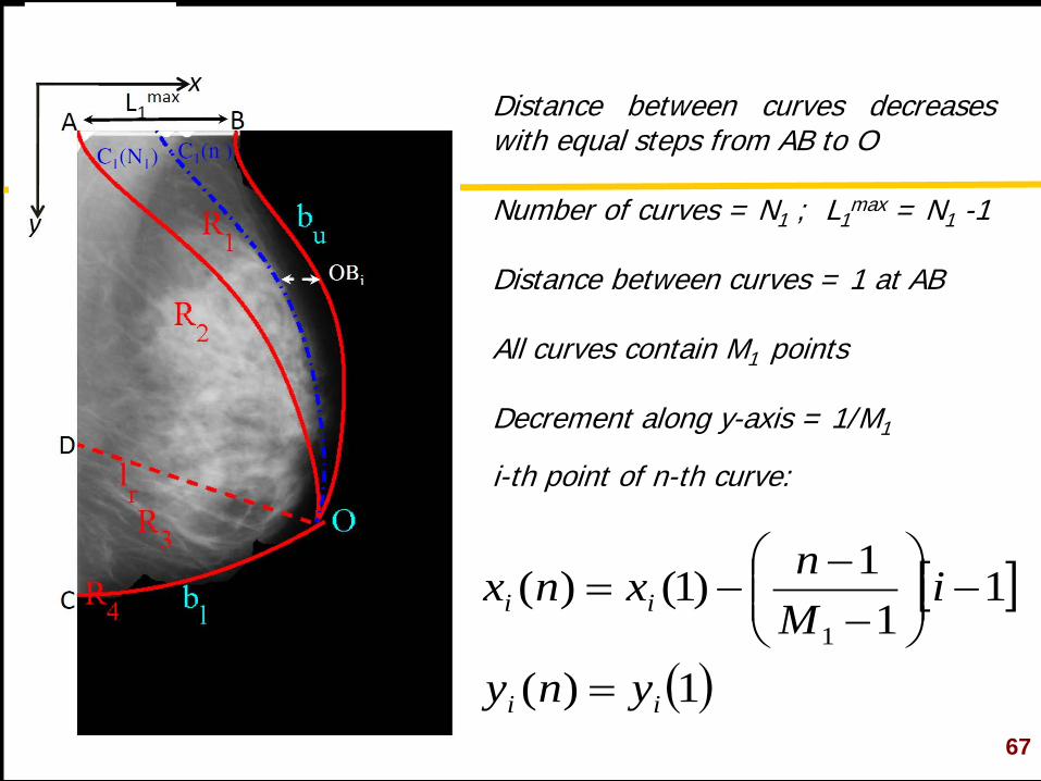
Distance between curves decreases with equal steps from AB to O Number of curves = N1 ; L1

max = N1 -1 Distance between curves = 1 at AB All curves contain M1 points Decrement along y-axis = 1/M1 i-th point of n-th curve:

[ ]

( )1)(

11

1)1()(1

ii

ii

yny

iMnxnx

=

−

−

−−=

67

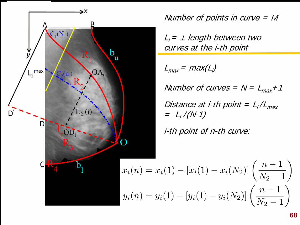
Number of points in curve = M Li = ⊥ length between two curves at the i-th point Lmax = max(Li) Number of curves = N = Lmax+1 Distance at i-th point = Li /Lmax = Li /(N-1) i-th point of n-th curve:

68

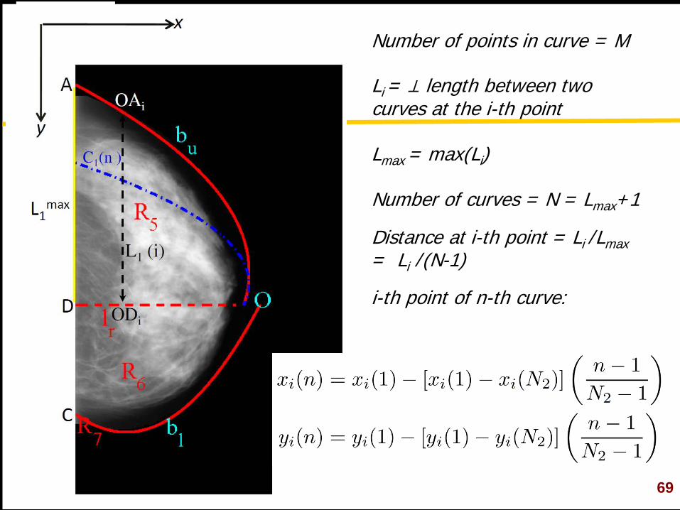
Number of points in curve = M Li = ⊥ length between two curves at the i-th point Lmax = max(Li) Number of curves = N = Lmax+1 Distance at i-th point = Li /Lmax = Li /(N-1) i-th point of n-th curve:

69

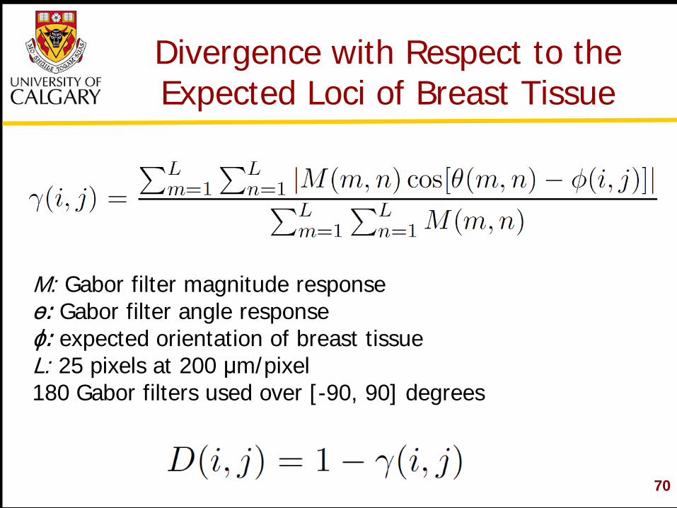
Divergence with Respect to the Expected Loci of Breast Tissue

M: Gabor filter magnitude response ɵ: Gabor filter angle response ɸ: expected orientation of breast tissue L: 25 pixels at 200 μm/pixel 180 Gabor filters used over [-90, 90] degrees

70

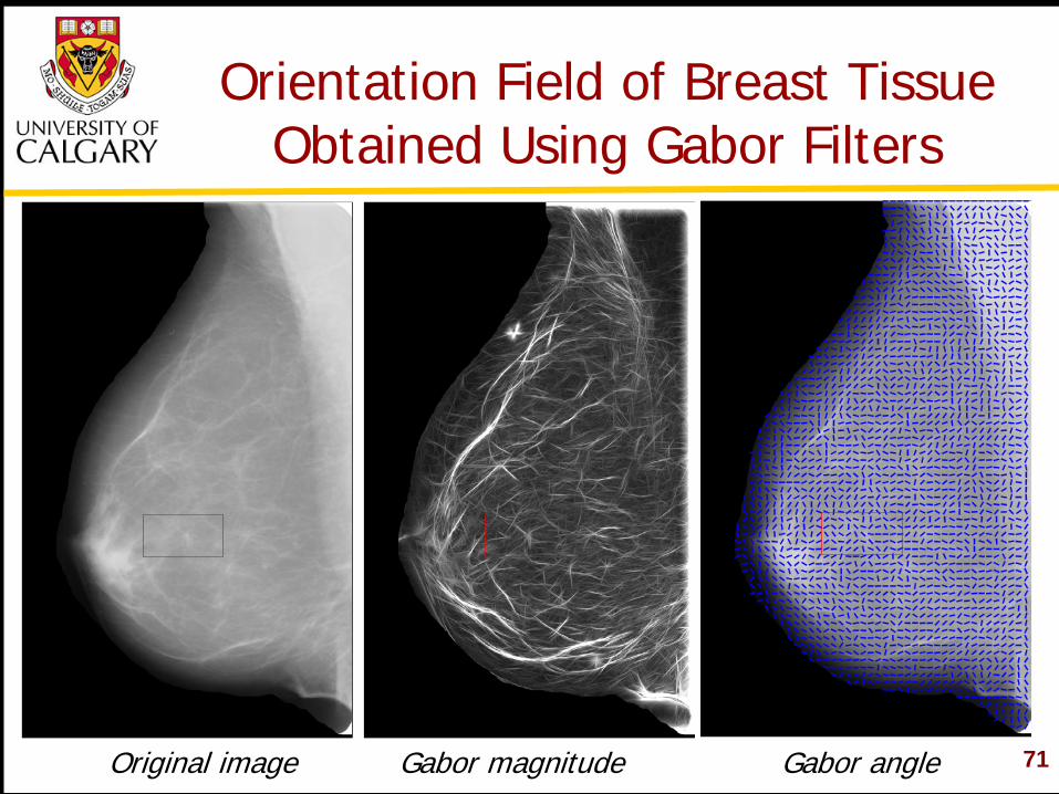
Orientation Field of Breast Tissue Obtained Using Gabor Filters

Original image Gabor magnitude Gabor angle 71

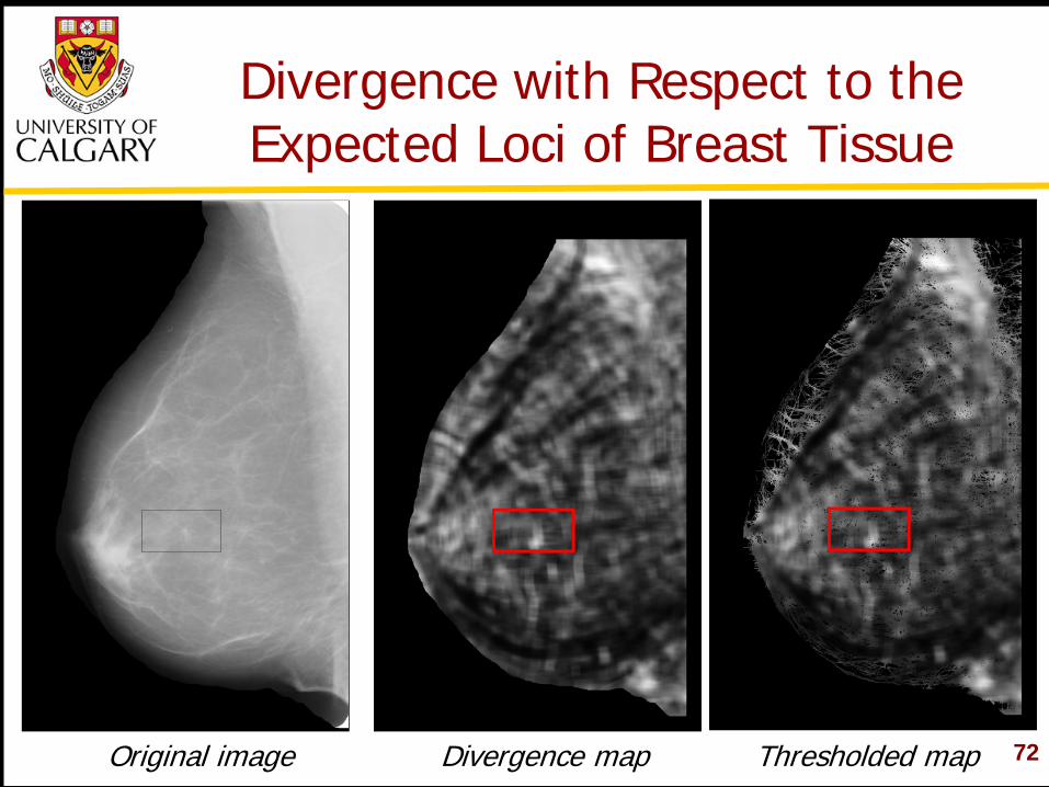
Divergence with Respect to the Expected Loci of Breast Tissue

Original image Divergence map Thresholded map 72

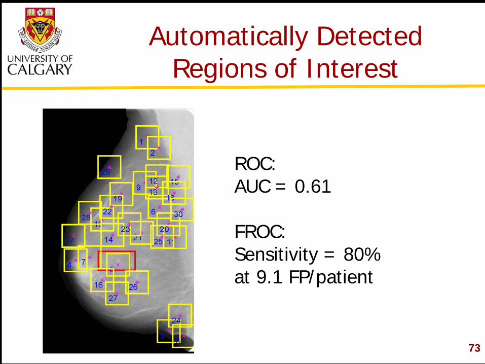
Automatically Detected Regions of Interest

ROC: AUC = 0.61 FROC: Sensitivity = 80% at 9.1 FP/patient

73

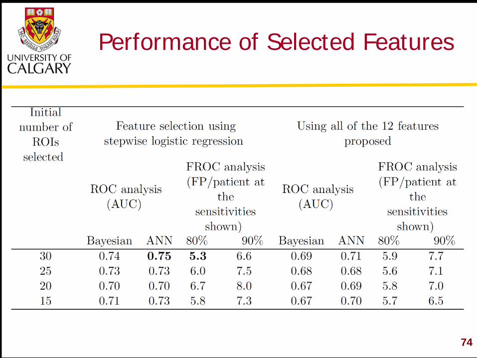
Performance of Selected Features

74

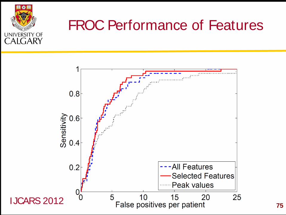
FROC Performance of Features

75 IJCARS 2012

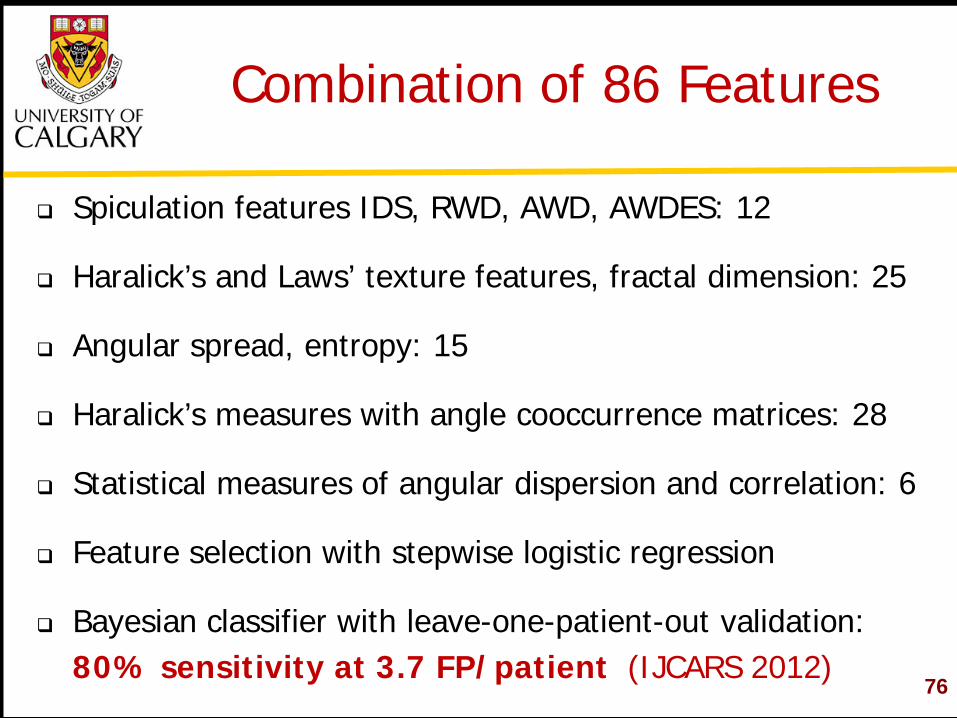
Combination of 86 Features

Spiculation features IDS, RWD, AWD, AWDES: 12

Haralick’s and Laws’ texture features, fractal dimension: 25

Angular spread, entropy: 15

Haralick’s measures with angle cooccurrence matrices: 28

Statistical measures of angular dispersion and correlation: 6

Feature selection with stepwise logistic regression

Bayesian classifier with leave-one-patient-out validation: 80% sensitivity at 3.7 FP/patient (IJCARS 2012)

76

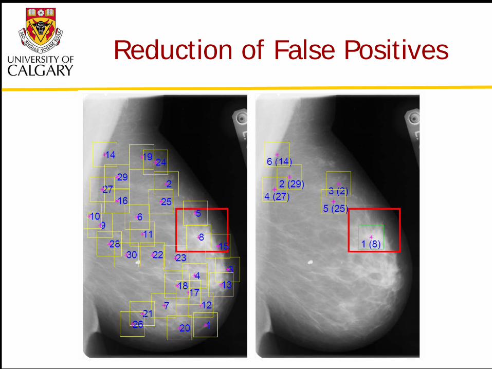
Reduction of False Positives

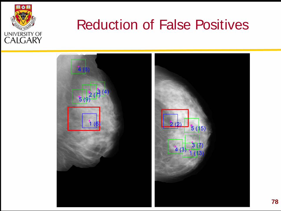
Reduction of False Positives

78

“Our methods can detect early signs of breast cancer 15 months ahead of the time of clinical diagnosis with a sensitivity of 80% with fewer than 4 false positives per patient”

Conclusion

Future work:

Detection of sites of architectural distortion at higher sensitivity and lower false-positive rates Application to direct digital mammograms and breast tomosythesis images

79

Natural Sciences and Engineering Research Council (NSERC) of Canada

Indian Institute of Technology Kharagpur Shastri Indo-Canadian Institute University of Calgary International Grants Committee Department of Information Technology, Government of India My collaborators and students: Dr. J.E.L. Desautels, Dr. S. Mukhopadhyay, N. Mudigonda,

H. Alto, F.J. Ayres, S. Banik, S. Prajna, J. Chakraborty http://people.ucalgary.ca/~ranga/

Thank You!

80