CHAPTER III

I. TRADE MODEL WITH INCREASING RETURNS TO SCALE, ZERO PROFIT AND THE COBB-DOUGLAS UTILITY FUNCTION

Recent development of trade theory in the area of market structure,

returns to scale,etc have enhanced our understanding of the cause of trade. While

writing the theory of factor proportion early in 1933. Ohlin pointed out that

economies of scale in production provide an incentive for international

specialization and trade, even in the absence of cross-country differences in factor

endowment.

Using the increasing returns to scale production functions of both X and

Y industry which we've got earlier in the introduction part, we will try to show

that both factor endowment and returns to scale play an important role in

deciding the trade pattern under certain conditions.

Unlike the case of perfectly competitive and constant returns to scale

where there is no clear focus on firms in the market, we will discuss some issues

of individual firrns in the oligopolistic structure of increasing returns to scale. In

the following, we assume general production function with increasing returns to

scale, zero profit in the long run and Cobb-Douglas utility function for knowing

the trade pattern in an autarkic general equilibrium model.

Production function of a representative firm in each of the two industries

producing goods X and Y are :

28

(1)

Where X and Y are firm outputs, Lx and LY are labour units employed, kx and ky

are capital labour ratios, rx and ry returns~to-scale parameters in the two

industries respectively. For the assumption of increasing returns to scale, ri(i =x,y)

is strictly larger than one, but less than 2 for profit maximization. This point will

be elaborated in the next part and also in the appendix. (0 < ri < 1) represents

decreasing returns to scale.

Let rr x and rr Y be the profits of representiye firms, defined as

1tx = Px(X,Y)X - WLx - rKx

(2)

Where Kx and~ are capital stocks, Px,Py prices and W ,r nominal wage rate and

- -rental price of capital, X = ~X and Y = I; Y are total outputs in the two

industries. Factor prices are assumed to be the same in the two industries as

there is no imperfection in the factor markets. The product markets are assumed

f0 be oligopolistic. The firms in each industry produce a homogeneous product

nnd follow Cournot·type conjectural variation in their profit maximizing

- -behaviour. In other words, dX/ dX = d Y I d Y = 1 . At the firm level decision-

- -making X and Y are assumed t() have no effect on PY and Px respectively.

29

Maximizing *the first profit function in (2) with respect to Lx and Kx and the

second with respect to LY and KY, we get

a1tx = [P~(X)X + 'px(X)]XL = W aLx

anx = [P~{X)X + Px(X)]XK = r aKx

a1ty = (P~(Y)Y + Py(Y)]YL = W aLy

a1ty = [P~(Y)Y + Py(Y)]Y K = r aKy

(3)

Wher~ Xi and Yi(i=L,K) are the marginal products oflabour and capital in the

two industries, which may be written as:

rx-1 1\ XL = Lx (rxf - kxf,

Y - Lry-lh' K - y

(4)

Expressing the marginal revenue terms m equation (3) m terms of pnce

elasticities, we get

*

I - 1 Px (X) X+ Px = Px(l---)

exnx (5)

Further details are given in the appendix where second order conditions are discussed

30

Where nx = X/X and ny = Y /Y are the numbers of identical firms in the two

- P aY P industries respectively and e = - ax . ~ and e = -- .! are the market

X apx X y apy y

de mend elasticities. The number of firms is determined in a situation where each

firm earns zero profit in the long run. Using (2),(3),(5) and the Euler's law we

get

,, = P,(XJx{l-r,(l- e,lnJ} ~ 0

", = Py (Y) v{l-r,( 1 - e,ln,)} = 0

This gives us

i = X,Y

(6)

6(a)

We assume that the social utility functiton is Cobb-Douglas and therefore the

demand elasticities, € x and EY are unity. Thus, the number of firms is uniquely

determined by the returns-to- scale parameters:

ri n. = -- i = X, Y 6(b)

1 r.- 1 1

In this model ri is strictly greater than one. The number of firms is inversely

related to ri. For instance, if ri is close to unity, say 100/99, the number of firms

will be 100. ni is infinitively large in the constant return-to-scale case. We also

assume ri to be less than or equal to 2. For the sake of simplicity we do not

impose any integer constraint on ni. Since ri is a parameter of the model, its

values can he S0 chosen that ni ·iS an integer.

31

As the factor marginal productivity should be equal to the factor price for

firm's profit maximization, we use (3), (5) and (6) to get

p Py 2X = -YL =W r L ry

X

(7)

p Py 2X = -YK = r r k ry

X

We get the factor price ratio ( w) in each X, Y industry

W r/ -f'kx r h- h'k· (&) = - = = y y

r f' h1 (8)

Now, we turn to the demand side for knowing the price ratio. Maximizing the

Cobb-Douglas Utility Function

U = D" DP X y

We get

etDa-1D 11 -J..P = 0 X Y X

AD"DP-l_).p = 0 tJ X y y

D P +D P =I X X y y

Where ). is the Lagrange multipli_er.

I = National Income

Di =Demand, i = X,Y

In a closed economy, Dx = X = nxX ; Dy = Y = ny Y

From the above equations, we get

~ Dy = px p Dx py

32

(9)

9(a)

P = Price ratio

p X nxX nxL:1 f(~) (10) = --=-=Y- = y ex y nYY nYL;rh(~)

Where, ~ = y a

We get the following from the equility of marginal value productivity of capital

in (7) after using the expressions of marginal product of capital in( 4) and price

ratio in (10)

f l n h 1L X X

= y rxf nyryhLY

For rewriting Lx/LY' we use full employment condition.

( L +L = L

X y

- -LX~ + Ly~ = K

-L

X

Px = -=- ' L

-L

P = ...2. y -

L

( 11)

11(a)

Now, we have seven equations, 6-(a),(8),(10),(11) and 11-(a) and seven

unknowns kx ky ,px, pY' P, nx and ny for solving our closed equilibrium.When we

solve the above, equation ll(a),, we get

Using pj Py• we rewrite the above equation (11)

f I = y hI p x = y hI (ky-k)

ri ryh Py r~ (k-kx)

33

(12)

we get, ll(b)

Therefore, we get the two reducep form equations (8) and ll(b) in terms of the

factor endowment ratio, k to solve for kx and ky

We rewrite the equal factor price equation (8) as:

r ,.f - k,.f 1

f' Therefore,

f r --k = w

X f'. X

or

w + k ri

--X f'

or 1 f' --- --

w+k X ri

h -k = w r-y h' y

w +k = r)l y h'

1 h' --

w+~ r)l

8(a)

(13)

\Ve rewrite the equal marginal capital productivity equation ll(b) with the help

of(13).

f1(k- kx) = Y h 1~ -k) = (k-k.~) = Y (~ -k)

ri r)l (w+kx) (w+~) ll(c)

Let's find the relationship between labor ratio in X industry (Px) and that of Y

industry (Py) using (13).

=

34

k-k X 1 k-k w+k

X y = = y • ky-kx • W + ~

1 (A) +ky = -p -­

y y (&)+~

We get

w+k YPx = P ____r

Y w+k X

•

by (12)

(14)

We define the elasticity of factor substitution ( ai) with respect to factor price

ratio (w).

ak, w w a.=-.-=---1 aw ki kiw'(ki)

= x,y .(15)

Let's differentiate the changed equal factor price ratio equations 8(a) and equal

marginal capital productivity condition ll(c) using the above equations.

8(a)

By differentiation,

Using the definition of elasticities of factor substitution (15),we get

We change the above equation into variational form with an asterisk denoting

relative rate of change

35

(16)

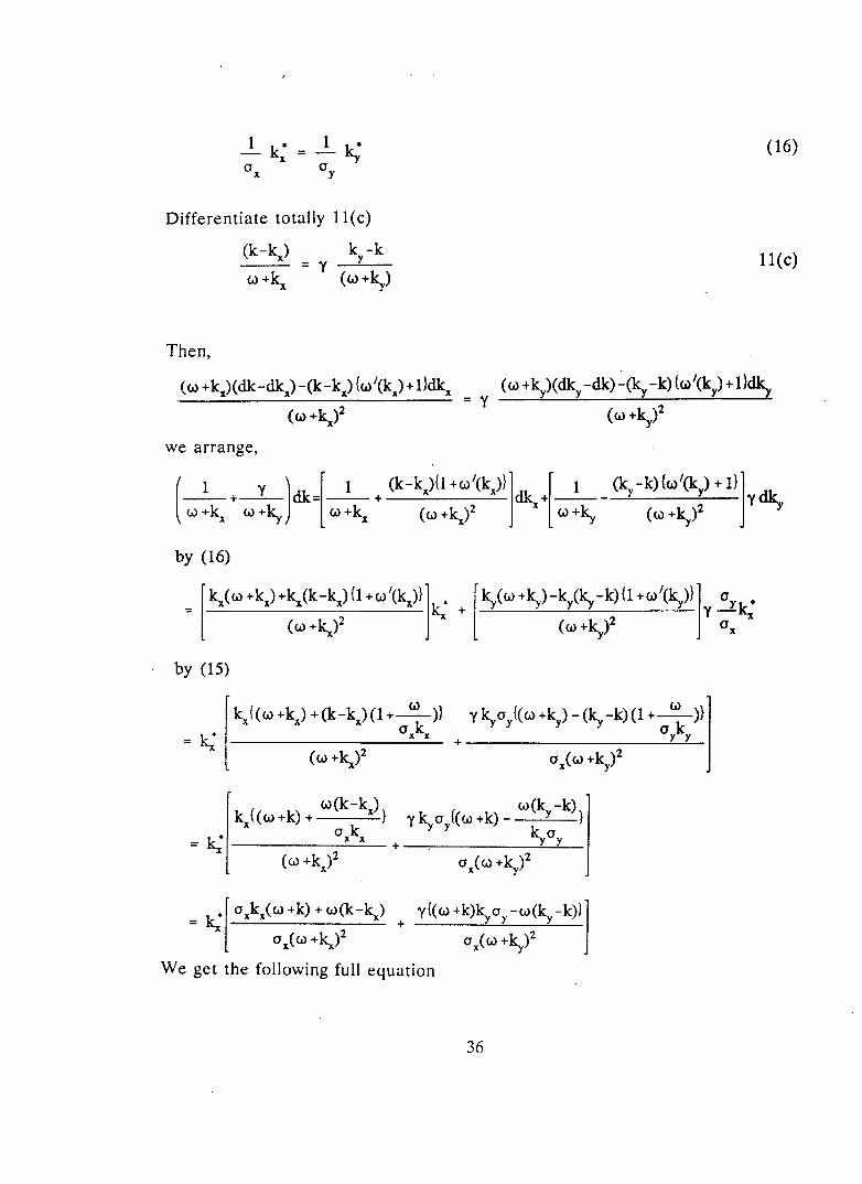
Differentiate totally 11(c)

(k-k) k -k __ x_ = Y ___..!....Y_

U> + kx ( U> + ~) ll(c)

Then,

(w +kx)(dk-dkx) -(k-kx) {w 1(kx)+ l}dkx = y (w +ky)(dky -dk)-~ -k) {w'(ky) + l}ill).

(w+~)2 (w+~i

we arrange,

by (16)

= [ ~(w +kx)+~(k-~){1 +w 1(~)}]~ + [~(w +~)-~(~ -k){1 +w'(~)}ly oYI<

(w+~i (w+~)2 ox

by (15)

::::; k. X

kx{(w+kx)+(k-kx)(l+ 0;x)} y~oy{(w+~)-(~-k)(1+

0: )}

--------- + y y (w +~)2

= ~r oxkx<w +k) + w(k-k) + y{(w +k)~oy -w(ky -k)}l

ox(w +k,i ox(w +ky?

We get the following full equation

36

We assume in the above equation (17)

. k ' yk· S=--+--

w+kx w+~

Z = [ oxkx(w +k) + w(k-kx)

ox(w+~?

Let us know the changing pattern of capital-labour ratios k·, kx. and ky.

k yk S=--+-->0

W+kx W+~

kx(w +k) w(k--k) oyky(w +k) w(ky-k) = + + y -y ----!..--

(w+kx)2 ox(w+~)2 ox(w+~)2 ox(w+ky)2

by ll{c)

Because, kx ~ k e ky and (k - kJ (ky-kJ > 0, Z is larger than zero (Z > 0)

37

~ = ~ k* > 0 z

(18)

~ = ~~ k* > 0 if k* > 0 ox z

Thus, kx·· ky. and k. have the same sign, whether plus ( +) or minus(-) .

. And, let us kqow the relative ,size of variables k·, ky·· kx.

For that purpose , we work out (Z - S)

Z _ S = kx(w+k) +y oykiw+k) + w(k-kx)(ky-kx) __ k __ _____y!_ (w +~)2 ox(w +~)2 ox(w +~)2 (w +~) w +~ U> +~

=

We reformulate the above equation in the following way:

38

Again, (Z - S)

=

(by 11-c)

1 a w(k-kx)(kx-~)(1--) yk (w+k)(2-l)

ox Y a = ------ + _____ x_ (19)

Then, we get the following results by using (18) and (19)

(i) k. > k. X if ox < 1 and ay ~ ox

( ii) k. < k. X if ax > 1 and ox ~ ay

(iii) k. = k. =~ ifo =a =1 X X y

39

In case (i) Z > S ; in case (ii) Z < S and in case (iii) Z = S,

So far, we tried to know the sizes of the change of capital-labour ratios

(~ ,k· .~) using the elasticities of factor substitution in both industries (ax,ay)

in our limited assumptions.

Using the equations which we have got so far, we try to know the relation

between price ratio (P.) and capital-labor endowment ratio (k.)for the

verification of trade pattern.

From the price ratio equation (10)

r, r,f k 0 x Lx ( x)

-r Lx'f(~)

~ - n L:'f(k)

r -1

p X nx· = = y = y X X = y

px -y nYL;yh(~) r r

n/L/h(~)

r -1 n .. X

= y -r L/h(~)

r -1 nr y

r -1 nr y

= y

r -1-r n Y L .. £(k)

Y X X

r -1-r nx .. L/h(~)

= y = y

We take log on both sides,

logP = logy+ (ry -l)logny- (rx -l)lognx + (rx -rY)logL +rxlog Px

-rylog Py + logf -logh

Totally differentiating and writng in variational form and remembering that nx

and ny.are uni9uely determine~ by rx and ry.

40

P* = (r -r)l:+r p*-r p*+C-h* X y X X y Y

(20)

. We know that the rate of change of price ratio (P*) depends on the variation rate

in the total labor (L *), the labor ratio in X industry ( Px "), the labor ratio in Y

industry ( Py·), productivity in X industry (f"), and productivity in Y industry (h *).

Let us look into (rxPx. - rypy*) in equation (20).

From the full employment equation (12)

k -k p X = ___.:._Y -

~-kx

Let us take the log function and by differentiation.

log Px = log (ky- k) - log (ky - kJ

~-dkx_

ky-~

• dk -dk Px = --'Y __

~-k

= (~~-+ k -k

y

(by 18) ...

(~ .5: _§_ - k) = ox Z

~-k

we define S/Z = m

. . (<y m-kl r~ :y -~ )~ Px = X - X r& k*

~-k ~-~

41

(12)

(12a)

And,

k-k X p =--

y ky -kx

Let us again take the log function

log Py = log (k - kx) - log (ky - kJ

Let's differentiate and with varia~ion form,

• dk -dkx dky -dkx Py = k - ~ - k) - kx

k-k X

k-km = k* X

k-~

We substitute (12a) and (12b) into (rxPx. - ryPy.)

rx(~ aYm-k) = k* __ a..::...x __

ky-k

And (-h. ' f 1dk

X h 1dk

- __ Y = k f'dk X X

f h

(12b)

(20a)

Equation (20) and the subsequent results show that a simple relationship between

p and k, which is the basis for a Heckscher-Ohlin type trade pattern, does not

exist in this model. We have therefore to introduce simplifying assumptions. Let

the elasticity of factor substitution in both industries (ax, ay) be the same and

equal to one (ax = ay = 1), then S equals Z (S = Z) and m = 1, kx* = ky* = k*

follows.

Then, rx Px. - ryPy• is reduced to zero.

r p • - r p • = k • (r - r + r - r ) = 0 xx yy y X X y

The price ratio change (20) is reduced to

P* = (r -r) L • + f* - h • X y

And, we get by (20b)

P*=(r -r)L*+(rxkx- rykylk* X y (A)+~ (A)+~

(21)

If suppose, the return to scale is the same in both industries (rx = ry).

Then, the above p• equation is reduced to

p * : f X x-y y X y k * : f X y k * {

k w + k 1c- - wk - k k } { w(k - k ) }

x (w+kx)(w+~) x (w+~)(w+~) 21(a)

P has the positive relation with k when the capital intensity in X industry is larger

than that of Y industry. So, we know that the traditional Heckscher- Ohlin type ' '

trade pattern is likely to be observed in the above situation.

But, when the returns to scale are not the same in the industries, p* is

determined by both the change of whole labor (L *) and capital labor endowment

ratio (k*)

43

= (r _ r ) L • + x x x x y y y y x y k. - {r k w +r k k - r k w - r k k } X y ((A) + ~) ( (,.) + ~)

(22)

with k • > 0 and L • ~ 0 p• > 0

p· and k • have positive relation if return to scale and capital intensity in X

industry are larger than those of y industry. We know that the Heckscher-Ohlin

type trade pattern is still valid with more constraints than in the traditional

model.

The Heckscher-Ohlin trade pattern is likely to be observed provided that

(i) the returns to scale in the capital- intensive industry is at least as strong as

that in the labour intensive industry and (ii) the capital-abundant country is at

least as large as the labour abundant country in terms of the size of its labour

force.

If, however, k • = 0.

then , p• = (r -r )L • X y (23)

This means that trade between two countries that are identical in relative factor

endowments but different in size is likely to be determined by the returns to scale

44

factor. The larger country is likely to have comparative advantage in the product

whose returns to scale is stronger and the smaller country will have comparative

advantage in the product whose returns to scale is weaker.

The analysis upto this point does not really determine the pattern of trade.

One has to look into the integrated world economy for determining comparative

advantage. Our purpose has been to show that an unambiguous relat~onship

between the autarky price ratio and factor endowment ratio does not e1nerge

unless we assume that ax = ay = 1. In what follows we formulate a model with

Cobb-Douglas production functions and discuss the equilibrium in the integrated

world economy.

45

II. INTEGRATED WORLD TRADE MODEL WITH COBB-DOUGLAS PRODUCTION FUNCTIONS AND INCREASING RETURNS TO SCALE

In the following, we extend the prevwus closed economy into open

economy which includes foreign country and try to know the trade pattern in the

integrated world formulation ori~inated with Dixit and Norman(1980). We use

the Cobb-Douglas production function in place of general production function of

the preceding part of this chapter. The production function of a representative

firm in each of the two industries producing X and Y goods are:

.X = L «xK Px = L "x + P1 ( KXJP• X X X L

X

r. = a. + A.> 1, I I 1-' I i=x,y

(1)

From the X, Y functions, the marginal products of labour and capital may

be written as:

XK = L:•pxk:x-1 ~ = PxL~~-1~.-1 X

(2)

For profit maximization of a representative firm with respect to its factors,

Land K:

46

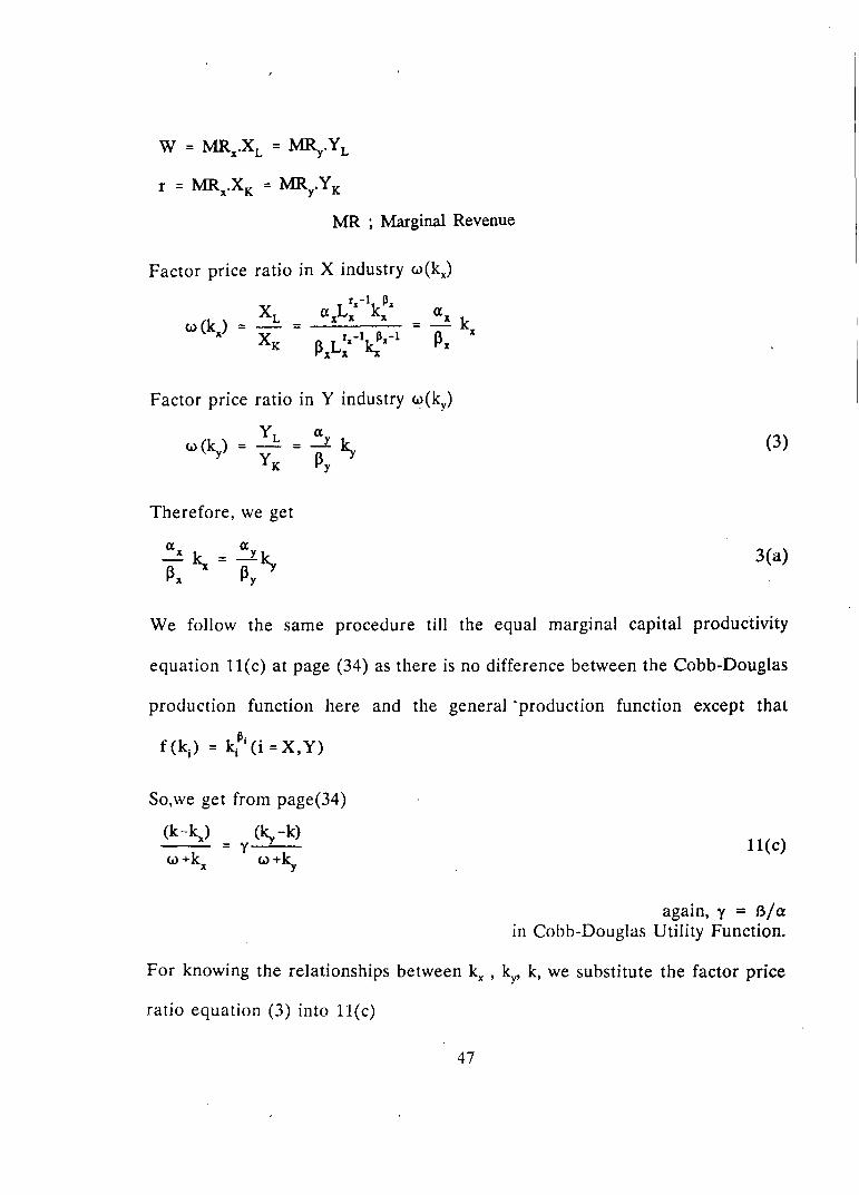
r = MRx.XK = MRY.Y K

MR ; Marginal Revenue

Factor price ratio in X industry w(kJ

XL w(k) = - =

X X K

Factor price ratio in Y industry U?(ky)

w(~) = YL = ~ ~ YK ~y

Therefore, we get

(3)

3(a)

We follow the same procedure till the equal marginal capital productivity

equation ll(c) at page (34) as there is no difference between the Cobb-Douglas

production function here and the general 'production function except that

f(ki) = ~~1 (i =X,Y)

So,we get from page(34)

(k-~) = y (~ -k)

w+k1 c..>+~ ll(c)

again, y = B/a in Cobb-Douglas Utility Function.

For knowing the relationships between kx , kY' k, we substitute the factor price

ratio equation (3) into ll(c)

47

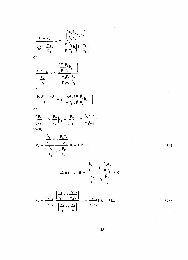
or

k- k X

or

or

(~ + Y ~)kx = (~~ + Y Pxay)k rx ry rx axry

then,

Px Pxay - +y--

~= rx axry

k = Hk (4) . Px

+ y~ rx rY

Px Pxay - +y --

where H = rx axry

> 0 ' Px p

+ y _L

rx rY

4(a)

48

where , J..

And, the factor price ratio( w) is:

(5)

~. ~.", l -+y--

where, J "x rx axry > 0 =-

Px (~•r!r] rx ry

We come to know that the factor price ratio ( w) and the factor endowment ratio

(k) have the positive relation. When we introduce the world which consists of

only two countries, Home (h) and Foreign Country (f) into our model, we get

K 8 = Kh + Kt

L8 = Lb + Lr

then

g:Global

Kb +Kt Kb Lh Kr Lr k = = -.- + -- = p k + p k

8 L LL LL hh tt g h g f g

Where ph = ~/Lg and Pr = Lr/Lg.

Therefore,

~ ~ kg ~ kc

(6)

Then, we can draw the following straight line through origin between w and k

according to (5)

49

k

Before trying to find the equilibrium price ratio of X.Y goods for the

closed economy, let's find out the labour ratio in X. Y industry ( Px• Py). From the

full employment condition ( 12) at page(33 ), we get.

k -k P - y

x ~-kx

k-k X

Py = --~-kx

by (12)

We calculate

6(a)

J3x J3x«y J3y 1_ P.a,) --+y-- y-

k-~ = k 1 -rx «xry

= k rY «xJ3y

~X J3 J3x J3 --- +y-L + y .:J..

6(b)

IX rY rx ry

k-~ = k 1 6(c)

50

Therefore, the labor ratio in X industry ( pJ is: ' '

Px =

(~ + y Pxcxyl rx CXly

(7)

Px is a constant because all (rx, ay, ~x· .. ) are parameters.

Therefore, Py = 1 - Px = constant also,

Next, we try to know the demand funtions of X.Y goods using Cobb-

Douglas Utility Function.

Again, using Lagrangian from the closed equilibrium model 9(a) at page(32)

(X Dy p X - = p Dx py

or,

Dy p px

=- -D (X p X y

We substitute the above demand DY into the Income equation.

p px Z (Income) = D P + - - DxPy

X X (X p y

51

Then, the demand functions are;

Dx z (X (8)

= --px cx+P

D z _P_ = y py cx+P

We assume the price of X goods as numerate (Px= 1), then, the price ratio(p)•

Then, the demand functions (8) is rewritten as follows.

D=-p_z y

Now, we try to get the national income (Z) from the factor market.

w- r­Z=-L+-K

px px

~

Assuming the social Cobb-Douglas utility function and taking factor marginal

productivity with zero profit in the long run (7) at page(32), we get

r xk ~ Lrx-1 kPx-1 -=-Px

X X rx rf

w XL = ~ L:I-l~I = (9) p rx rx X

52

Then, the national income(Z) is;

z = ~ L:·-1~'L + .~x L:·-1~·-1i( rx rx

r -1

= Lr,£ k:'- 1n~·-r·(cxx~ +Pxk) rx

r, -1

= ~HP,-1n~-r·(cxxH+Px)Lr•kp• rx

We rewrite the demand functions Dx DY in the following way.

r1

-1 _ p _ P D = _p_ ~ HP.-1n 1-r.(cx H+P) L r1k 1 =C e•k 1

Y a+ p rx x x x p p

where,

Now, we get the supply functions of X and Y goods

X == n L r,kP. == n 1-r .. (L- )r• kp1 X X X X. X X

where p X

53

by (4)

8(a)

(10)

We've got the demand and supply of both goods.

Then, for Y goods(Dy = Y)

therefore,

pea = .A[<rx-rr>k<P.-P,.> (11)

= closed economy equilibrium price ratio

A > 0

We come to know that in the closed equilibrium, the price ratio depends on

eeuntry size (L) and capital-labour endowment ratio(k). In this model, the price

' ratio is independent of its output. This independence character has also been

shown in many other monopolistic competition models.

ANALYSIS OF INTEGRATED WORLD TRADE MODEL

We assume that the world (G) simply consists of home country (H) and

foreign country (F) and follow the way of what Krugman(1980), Lawrence &

Spiller ( 1983) had done in their integrated trade model. The foreign country

having the identical production functions has a closed economy equilibrium

similar to that, of the home country. And also, the world equilibrium shows the

same structure of relationships as in the home aswell as foreign country closed

equilibrium as if the world is a bigger country than either home or foreign

54

country. The world economy, ,being a closed economy, has perfect mobility of

both goods and factors within itself.

Using the relation between factor price ratio ( w) and factor endowment

ratio (k) in a closed economy from (5) extended to world equilibrium, let's try to

know the relation in our integrated world trade.

(&)h = J kh

h : home country, g : global

Then, we get

(12)

wh- wg = J(kh -kg)>< 0 , as, kh> <kg 12(a)

We know that if home country is capital abundant, the factor price ratio ( w) falls

when trade takes place as in the traditional Heckscher-Ohlin theorem. This of

course, presupposes that the integrated world equilibrium can be taken as the

free trade equilibrium-a proposition which we shall establish later.

Next, we try to know the tendency towards the equilibrium factor price

ratio. From the real factor price equation (9).

W = Closed economy equilibrium wage rate measured m terms of good X

= (XX (Lxtx-1 k:• rx

13(a)

55

Where,

<X 1 r 1 -1Hp• 1-r1 O Jx =- Px nx >

rx r = Closed economy equilibrium profit rate on capital

= HxcLt·-1kP.-1

Where,

= ~ p:·-1n~-\L)r.-1 HP.-1kP.-1 rx

Px r,-1 1-r, p -1 O H =-p n H • >

X X X

rx

13(b)

It may be mentioned here that since the number of producers in each

industry is uniquely determined by the returns to scale parameter, the two

countries as well as the integrated world economy will have the same number of

producers in each industry. It also implies that the degree of industrial

concentration is higher in the world economy than in either of the two counties

in their respective autarky equilibria. This is a special feature of our model which

follows from Cobb-Douglas utility function. But, Lawrence and Spiller(1983) have

used C.E.S. utility function in monopolistic competition model for getting

different results. We write the equilibrium wage rates of home country and world

as follows :

wh = Jx(L)~'-1k:· by 13(a)

w = J (L)r.-1 kP. g X g g (14)

56

When the home country is relatively labour abundant (kg > kh), the world

equilibrium wage rate may be higher than the closed equilibrium rate (Wg > Wh).

Therefore, after trade the real wage rises in the labour abundant country. But,

if the home country is capital abundant (kh > kg), then the sign of (Wh- W,) is

indeterminate and we can not s.ay that the real wage rate falls in a capital

abundant country after trade begins.

Likewise,

by 13(b)

(15)

Since 1 < (ax + .Bx) < 2, we also assume that .Bx < 1.

When the home country is relatively capital abundant (kh > kg ) and (.Bx < 1),

then world equilibrium return on capital may be higher than the closed

equilibrium rate. But, if the home country is labour abundant (kh < k ) and (.B . g X

< 1), then the sign of (rh - rg) is indeterminate. In both cases, a country's

abundant factor experiences an increase in its real reward after trade like in the

traditional Heckscher-Ohlin Theorem. But, nothing definite can be said about its

scarce factor's real reward.

57

THE TRADE PATTERN

We try to know the pattern of trade in the integrated world equilibrium.

From the closed economy equilibrium price ratio (11), we know that the product

price ratio depends on country size (L) and capital-labor endowment ratio (k)

unlike in the constant returns to scale model. We write home country(h) as well

as integrated world(g) equilibrium price ratio like:

ph = A(i)~' -ry k:• -~Y

p = A(i)r,-ry k~.-~,. g g g

(16)

In view of( 6) capital and labour in the integrated economy can be apportioned

between the home and foreign components in which case P g will be the free trade

terms of trade between the two trading countries with no international factor

mobility.

Firstly, let us know the sign of (Bx-By) in the above equation.

From 6(a)

then, Bx ay - ax BY > 0 or, Bx (ry-By) - BY (rx-BJ > 0 or, Bxry > Byfx

58

(17)

In other words, Bx and BY are proxies for capital labour ratios in the two sectors

provided that the returns-to-scale parameter is higher in the capital-intensive

sector.

We know from (16) that, when the returns to scale are the same in

both X and Y industry (rx = ry) and home country is relatively capital abundant

(kh > kg), then the integrated price of capital intensive goods (kx > ky, Bx > By)

might be higher than the closed economy equilibrium price (pg < ph). Then the

traditional Heckscher-Ohlin theorem holds.

But, when the returns to scale are not the same in both industries

(rx ,. ry), then the H-0 theorem may not hold. If suppose, the returns to scale in

X industry is stronger than Y industry (rx > ry, kx > kY' Bx > By) and there is no

difference in capital endowment ratios between countries (kh = kg = kr), then the

world integrated equilibrium price of X goods might be lower than that of closed

equilibrium price (Pg > Ph).

Now,let us compare the home equilibrium price ratio with foreign price ratio.

ph = A(L)~'-rY k:x-Py

Pr = A(L);·-rr ki·-Py (18)

If suppose, the home country is simply bigger than foreign country in terms of

population size (Lh > Lr), but both countries have the same capital labour

endowment ratio as before arid (k > k, r > r and B > B) then the price of X y X y X Y'

capital intensive goods in home country (1/Pg) might be lower than that of

59

foreign equilibrium price (Ph > Pr). Therefore, we come to know that a country

larger in size will have comparative advantage in the capital intensive goods of

which scale economy is stronger. But in free trade, the price of the product will

decrease in both countries.

1 I 1 -< -<- 18(a) pg ph pf

We assume that this outcome is due to world wide production opportunities of

economies of s~ale. In this mod.el, the smaller country will gain more because it

import goods at cheaper price than autarkic price of import-competing goods and

export the labour intensive goods at a higher price than the autarkic equilibria,

whereas the large country exports at a price less than its autarky price.

Now, we try to explain the pattern of trade using excess demand function.

EDY = world excess demand for Y good(world consumption- world production)

J {L)r~ kll~ (L)r1 1r~1 ] = Ll ~ h + ~ nt - C •[ L~r k:1 + L;r Icir) = 0

Then, we get free trade equilibrit.Im price ratio (Pe)

pe = C(~x~x+L;x~x) (19)

c·~rk:r +L:1 ~1) Substituting the free trade equilibrium price ratio ( 19) into the domestic demand

function of Y goods 8(a), we get home country excess demand of Y good (EDyh)

60

EDyh

LrYlr~Y 1+-f~_

~Yk!Y

L;x~x 1+-·--

~·~·

- 1 (20)

If (kr > kh, bJ.It Lr= ~). then, th~ excess demand of Y goods equation(20) is

changed like

EDyh < 0 20(a)

When the size of population is the same in both home and foreign countries

(Lr = L11 ), but the foreign country is more capital abundant than home country

(kr > k11 ), then the excess demand of Y goods at home country might be less than

zero (EDyh < 0), that is, the home country exports the Y goods which are labour

intensive.

Likewise, if(Lh > Lr, but kr = k 11), then again equation (20) is changed like,

( Lf ry - ( Lf r,

Lh Lb

I + ( ~:r > 0' 20(b)

61

1

When the size of home country is bigger than foreign country (L11 > Lr), but the

capital~lahour endowment ratio is the same in both countries, then the home

country exports the good in which scale economy is stronger as we sec in both

equations (18) and 20(b).

62