Chapter 6

Production Theory and Estimation

Production Theory and Estimation

Ch. 6: Production Function and Estimation Overview

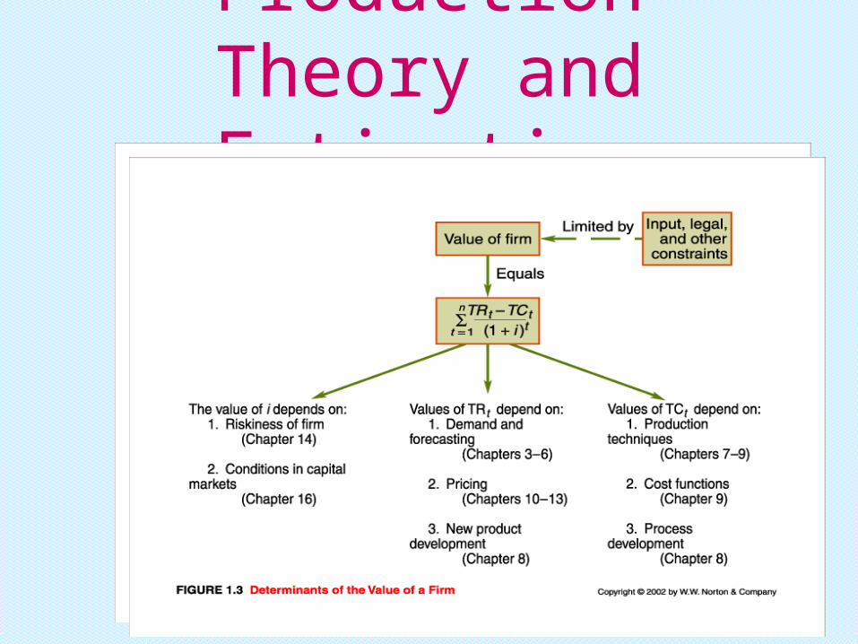
1. The main objective any business is to maximize profits (Value Maximization).

Profits = Revenues - Costs (Value) (P, Ad. Quality) (Efficiency)

Guiding Principles of Optimal Resource Use

1. The Single Case : Q=f(L)

Decision Rule: MRPi = MFCi => # 4,

MRPi=> marginal revenue product (MR) input i

MFCi=> marginal factor cost (MC) input i

What if MRPi > MFCi ?

Should we use more or less of the resource? Why?

Guiding Principles of optimal resource use-cont.

2. The multiple inputs case Q=f(L, K)

a. Least cost combination rule=> MPL/w=MPK/r #10

(This is a necessary condition for optimal input use)

What if MPL/w < MPK/r? Use more or less labor? Why?

b. Given the production function Q=f(L, K), the cost of hiring workers (w) and the cost of capital (r), and the firm’s cost outlay (C= wL+rK). The objective function of the firm may be to: Maximize Q s.t. C=wL+rK, or

Minimize C=wL +rK s.t. the constraint of producing a fixed Q

Sufficient Condition for Choosing the Optimal Combination of L and K

Optimal input use: MPL /MPK=w/r

(This rule a sufficient condition for optimal use).

What if MPL/MPK < w/r => use more what?

L

K

k2

L2

k1

L1

Q2Q1

Q3k3

L3

C1 C2 C3

1. Production is the process of transforming inputs (resources) into output of goods and services.

Inputs include land, labor including entrepreneurial talent, and capital.

2. a) Fixed inputs are those that can not readily be changed during the period under consideration.

Note: In the SR, we have both fixed & variable inputs

Variable inputs are those whose use changes as needed (Labor, utilities, etc.)

b) Short-run is the time period during

which at least one input is fixed.

Long-run is the time period during

which all inputs are variable.

3. A production Function shows the relationship between inputs and some output.

Qbooks =f(workers,machine,paper,ink,

others)

Qgraduation=f(faculty,facilities,personnel,

etc)

4. The short-run production function with one variable input(labor).

a) The total product of labor (Q) shows the different levels of output produced by different quantities of labor(capital is fixed).

Measures of Productivity

• The average product of labor(APL) measures output per worker

APL= Q/L measures production efficiency

The marginal product of labor(MPL)

measures the output produced by the last unit

of labor.

;MP Q LL / dLdQMPL /

- The output elasticity of labor (EL) measures the percentage change in output as a result of one percent change in the quantity of labor.

E Q L Q L L QL % / % / * /

MP APL L/

b) Short-run production of potatoes on one acre of land using labor as a variable input.

L Q(lb) APL=Q/L MPL= Q/ L EL=% Q/% L

0 0 - - -

1 3 3.0 3 1.00

2 8 4.0 5 1.25

3 12 4.0 4 1.00

4 14 3.5 2 0.57

5 14 2.8 0 0.00

6 12 2.0 -2 -1.00

Notice that the MPL is diminishing beyond

the 2nd unit of labor. Why?

5. a) Some measures of productivity:

-Output per worker (APL) =Q/L

-Marginal productivity per

worker(MPL)=ΔQ/ΔL

or dQ/dL

b) Factors which influence productivity gains:

Increase in the amount of capital available per worker(K/L)

Improvements in technology(the level of applied scientific knowledge).

Changes in institutional rule(union work rules

Changes in government statutes.

Demographic trends may be the driving force behind technological changes, work-rule modification(fast food tech, flexible work hours).

c) Importance of productivity gains:

-Increased profits for firms.

-Better standards of living for society.

6. The three stages of SR Production

See, p. 240a) Stage 1-The fixed factor of production is underutilized. As we add more of the variable input to the fixed input, productive efficiency increases. AP increasing, MP>AP, EL>1.

b) Stage 2-Represents a rational boundary of production. In our example, it occurs between 3 and 5 units of labor.

c) Stage 3-Total product is declining. Even if wage per hour is 0, a rational producer will not use more than 5 units of labor in our example (Refer to previous table).

Notice that the output elasticity of labor is negative in this stage i.e. EL< 0

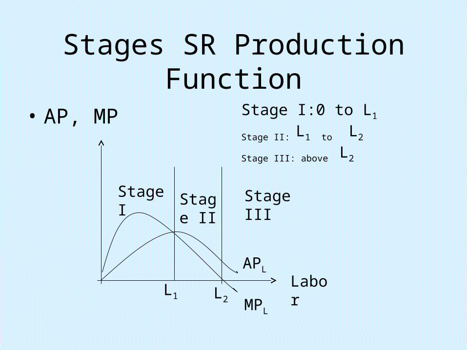
Stages SR Production Function

• AP, MP

LaborAPL

Stage I Stage II

Stage III

L1 L2

Stage I:0 to L1

Stage II: L1 to L2

Stage III: above L2

MPL

7. An optimal labor size will be employed when the marginal revenue product (MRPL) and the marginal factor cost of labor (MFCL) are equal =>MRPL = MFCL

MRPL = MPL * product price (=>DL)

MFCL = the additional cost of hiring an additional worker (SL)

Rule: MRPL =MFCL

Labor Units MPL MR=Price MRPL MFCL

2.5 4 $10 $40 $20

3.0 3 10 30 20

3.5 2 10 20 20

4.0 1 10 10 20

4.5 0 10 0 20

Optimal Units of Labor

MRP

MFC

Labor

MFCL

MRPL

3.5

$20

8. A production function with two variable inputs Q = f(L,K).

a) Iso-quant curve is a curve which shows the various combinations of labor and capital which yield the same level of output (see p. 243).

b) MRTSLK is the rate at which labor is substituted for capital. It represents the slope of the iso-quant curve (p. 276).

MRTSLK = - K/ L = MPL/MPK

Multiple Inputs Production Function

c) Ridge lines are lines which separate the relevant (negatively sloped) from the irrelevant portions of the iso-quants.

d) Iso-cost line is a line which shows the various combinations of labor and capital which entail the same total cost

Total cost(expenditures) = exp. on labor and exp on capital

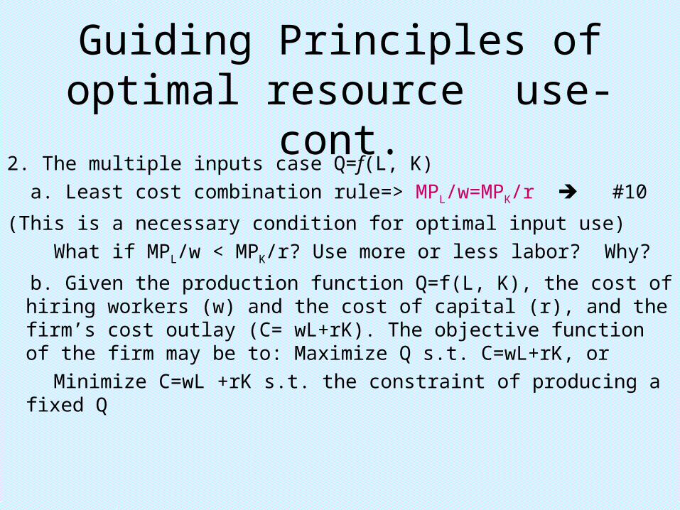
Guiding Principles of optimal resource use-cont.

2. The multiple inputs case Q=f(L, K)

a. Least cost combination rule=> MPL/w=MPK/r #10

(This is a necessary condition for optimal input use)

What if MPL/w < MPK/r? Use more or less labor? Why?

b. Given the production function Q=f(L, K), the cost of hiring workers (w) and the cost of capital (r), and the firm’s cost outlay (C= wL+rK). The objective function of the firm may be to: Maximize Q s.t. C=wL+rK, or

Minimize C=wL +rK s.t. the constraint of producing a fixed Q

Sufficient Condition for Choosing the Optimal Combination of L and K

Optimal input use: MPL /MPK=w/r

(This rule a sufficient condition for optimal use).

What if MPL/MPK < w/r => use more what?

L

K

k2

L2

k1

L1

Q2Q1

Q3k3

L3

C1 C2 C3

MRTSLK=ΔK/ΔL=MPL/MPK

K

L

Slope of Q1 at b => ΔK/ΔL=MPL/MPK=w/γ

Q1

b

C1L1

K1

Note: K1 and L1 are optimal mix of K and L

C2

Slope of Isocost equation=> K= C/r – wL/r =>w/r taking the derivative of K w.r.t. L

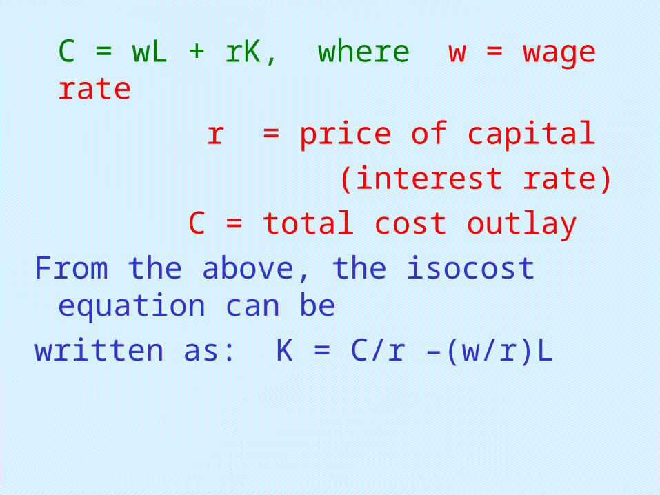
C = wL + rK, where w = wage rate

r = price of capital

(interest rate)

C = total cost outlay

From the above, the isocost equation can be

written as: K = C/r –(w/r)L

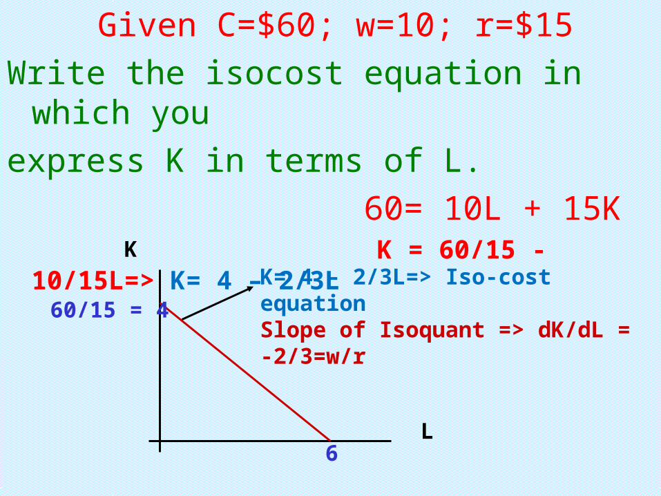
Given C=$60; w=10; r=$15

Write the isocost equation in which you

express K in terms of L.

60= 10L + 15K K = 60/15 - 10/15L=> K= 4 – 2/3L

K= 4 – 2/3L=> Iso-cost equationSlope of Isoquant => dK/dL = -2/3=w/r

L

K

60/15 = 4

6

9. An optimal input combination is obtained when a mix of resources (inputs) for which the MRTS is equal to the slope of the iso-cost line(the input price ratio).

MRTSLK=- K/ L=>MPL/MPK => slope of

isoquant

dK/dL = w/r =slope of isocost

Optimal point=> at MPL/MPK=w/r

Optimal Input Mix of K and L

E

F

L

K

Q1

Notice that only point D satisfies the optimal input combination. Why? P. 250

K

L C1 C2

At point D, 1. MPL/W=MPK/r =>LCC2. MPL/MPK=w/r => sufficient condition for optimal combination

D

A firm can minimize the cost of producing a given level of output or maximize the output for given cost outlay when MRTS = W/r. This equilibrium condition yields both production and cost efficiency.

10. An expansion path is a line which traces the least cost combination of inputs (i.e. MPL/w=MPK /r). P. 250

Note this takes place in the long-run when all production inputs can vary.

11. The effect of a decrease in the wage rate, the cost of capital remaining the same is the use of a labor intensive technique of production and vice-versa.

12. Returns to scale refer to what happens to output if all the variable inputs are changed by the same proportion (%) in the LR?

There are three possibilities:

a) Output can increase by the same percentage as inputs => constant returns to scale.

b) Output can increase by a greater percentage than the increase in inputs => increasing returns to scale.

c) Output can increase by a smaller percentage than the increase in inputs => decreasing returns to scale.(see p.255)

13. a) The Cobb-Douglas production (Q =AKaLb) is used to estimate production relationships.

b) Useful properties of the Cobb-Douglas production:

- MPK and MPL depend on the quantities of capital and labor used, respectively.

- The exponents of capital (a) and labor (b) represent the output elasticity of capital(EK) and labor (EL), respectively. EK = a; EL = b.

- The Cobb-Douglas production function can be estimated by linear regression by transforming it into:

lnQ = lnA + a lnK + b lnL

- The Cobb-Douglas production function can be easily extended to determine the contribution of several inputs.

Returns to Scale from Cobb-Douglas Production Function

• The sum of the exponents of the C-D represent returns to scale

• Given Q =AKαLβ, If α + β= 1, the production function exhibits

constant returns to scaleIf α + β> 1, the production function exhibits

increasing returns to scaleIf α + β< 1, the production function exhibits

decreasing returns to scale