Production Function Estimation with MeasurementError in Inputs∗

Allan Collard-WexlerDuke University

NBER

Jan De LoeckerPrinceton University and KU Leuven

NBER and CEPR

May 12, 2016

Abstract

Production functions are a central component in a variety of economicanalysis. However, these production functions often first need to be estimatedusing data on individual production units. More than any other input in theproduction process, there is reason to believe that there are severe errors inthe recording of a producer’s capital stock. Thus, when estimating productionfunctions, we need to account for the ubiquity of measurement error in capi-tal stock. This paper shows that commonly used estimation techniques in theproductivity literature fail in presence of plausible amounts of measurementerror in capital. We propose an estimator that addresses this measurement er-ror, while controlling for unobserved productivity shocks. Our main insight isthat investment expenditures are informative about a producer’s capital stock,and we propose a hybrid IV-Control function approach that instruments cap-ital with (lagged) investment, while relying on standard intermediate inputdemand equations to offset the simultaneity bias. We rely on a series of Monte-Carlo simulations and find that standard approaches yield downward biasedcapital coefficients. We apply our estimator to two standard datasets, the cen-sus of manufacturing firms in India and Slovenia, and find capital coefficientsthat are, on average, twice as large. We discuss the implications for productiv-ity analyses.

Key words: Production function estimation; measurement error

∗Contact information: collardwexler@gmail.com and jdeloeck@princeton.edu. We thank SteveBerry, Matt Masten, Shakeeb Khan, Jo Van Biesebroeck, and Daniel Xu, and participants of theCornell-Penn State Econometrics workshop for helpful conversations, and Daniel Ackerberg for shar-ing his code. Sherry Wu and Yiling Jiang provided excellent research assistance.

1

1 Introduction

The measurement of capital is one of the nastiest jobs that economistshave set to statisticians. (Hicks (1981) p. 204)

Production functions are a central component in a variety of economic analysis.However, these production functions often first need to be estimated using dataon individual production units. Measurement of capital assets poses a problem forestimation of production functions. More than any other input in the productionprocess, there is reason to believe that there are severe errors in the recording ofa producer’s capital stock. These errors are likely to be large, and are extremelydifficult to reduce through improved collection efforts since firms themselves havedifficulty evaluating their capital stock. Thus, when estimating production func-tions, we need to account for the ubiquity of measurement error in capital stock.This paper shows that commonly used estimation techniques in the productivityliterature fail in presence of plausible amounts of measurement error in capital.We show that using both investment and the book value of capital can correct thepresence of measurement error in the capital stock. This idea follows the standardinsight of relying on two measures of the same underlying (true) variable of inter-est, and using one of these measures as an instrument for the other.

The presence of substantial, or at least the potential of, measurement error incapital is reflected in a well-documented fact that when estimating productionfunctions with firm fixed-effects, capital coefficients are extremely low, and some-times even negative. Griliches and Mairesse (1998) state ‘’In empirical practice, theapplication of panel methods to micro-data produced rather unsatisfactory results: low andoften insignificant capital coefficients and unreasonably low estimates of returns to scale.”.One obvious other interpretation is that capital is a fixed factor of production, andtherefore the variation left in the time series is essentially noise. However, this alsoimplies that changes in capital, which is by definition equal to investment minusdepreciation, is heavily contaminated by measurement error. Indeed, Becker andHaltiwanger (2006) do an in depth study of measurement issues related to capi-tal, and find that different ways of measuring capital that ought to be equivalent,such as using perpetual inventory methods or inferring capital investment fromthe capital producing sectors, lead to different results for a variety of outcomes,such as parameter estimates of the production function, and the investment andcapital patterns.

2

The recent literature on the estimation of production functions (Olley and Pakes,1996; Levinsohn and Petrin, 2003; Ackerberg, Frazer, and Caves, 2015), has ex-ploited control functions to solve the problem of endogenous inputs. However,these control function approaches are difficult to reconcile with the presence ofmeasurement error in inputs. We propose an estimator that deals with the mea-surement error in capital, while controlling for unobserved productitvity shocks. Inparticular, we leverage the log-linearity from the Cobb-Douglas production func-tion and productivity process, to construct an estimator that jointly addresses thesesources of bias, is simple to use, and requires no additional data.

Related Literature

There has a been a long literature on the estimation and identification of produc-tion functions when a researcher has access to a panel data set of producers overtime (of a given) industry with information on output and inputs. Olley and Pakes(1996) (henceforth OP) and Levinsohn and Petrin (2003) (henceforth LP) have re-newed interest in addressing the simultaneity bias, due to the unobserved produc-tivity term ωit, when estimating the relationship between output and input. Morerecently Ackerberg, Frazer, and Caves (2015) (henceforth ACF) refined the preciseconditions under which these production functions are identified, and providedan alternative estimator. In a related literature, the focus has moved away from theclassic simultaneity problem to the one of unobserved prices, for both output andinputs (De Loecker and Warzynski, 2012; De Loecker, Goldberg, Khandelwal, andPavcnik, 2016).1

Van Biesebroeck (2007) evaluates the performance of various production func-tion estimators, including the so-called control function approaches, in the pres-ence of measurement error, although not with a specific focus on measurement er-ror in capital. He compares various methods in the presence of log additive mean-zero independent and standard normally distributed errors to all inputs, measure-ment error in output and input prices. While the focus of Van Biesebroeck (2007)

1In most settings, we observe firms charging different prices for their output, and paying differentprices for inputs, which leads to an additional complication since researchers typically only haveaccess to (deflated) revenues and expenditures on inputs. We believe this to be a very importantconcern, but we abstract away from this issue in this paper. In other words we start our analysis byhaving correctly converted the revenue and expenditure data to the comparable units in a physicalsense. This is precisely the setup of Ackerberg, Frazer, and Caves (2015). Of course, to the extentthat input prices vary across firms, and are not correlated with the actual levels of input choices, ourapproach is relevant.

3

is on the bias in the estimated coefficients, we provide an estimator that is robustto the presence of such measurement error, in the context of endogenous inputchoices.

Kim, Petrin, and Song (2016) also study the identification of production func-tion with measurement error in inputs, and suggest an estimator that leverage re-cent research in the econometric literature on non-linear measurement error mod-els. Their paper relies on different condition than ours for identification, essentiallyleveraging the fact that the classic models of investment and input choice used forproduction functions, famously outlined in (Olley and Pakes, 1996), is a first-orderMarkov process. Thus further temporal dependance in observable transitions canbe used to structure the measurement error in capital (similarly to Hu and Shum(2013)). This estimator is more complex, which explains why, to our knowledge,their estimator has not yet been used. In contrast, our estimator is simple to pro-gram and use with standard statistical software packages.

2 Sources of Measurement Error in Capital

In this section we discuss the potential sources of measurement error in capital, andhow we incorporate measurement error into estimation of the production function.This discussion leads to, what we believe, to conclude that investment is a naturalinstrument for recorded capital.

2.1 Construction of Capital Stock: Book Value and Perpetual InventoryMethods

Capital stock is typically measured in two ways, using either book value, or theso-called perpetual inventory method (PIM, hereafter). The book value of capitalis measured using direct information on the value of capital, as recorded in a firm’sbalance sheet. The PIM requires data on investment, and recorded depreciationsto construct capital stock. Of course, both of these approaches are related, sincethe book value of capital is typically the outcome of firms themselves applying thePIM in their internal accounting. PIM is the most common approach to constructcapital stock series, see Becker and Haltiwanger (2006) for an excellent overview.In essence this approach measures the capital stock of a particular asset Ka using:

Kat =

∞∑j=0

θajtIat−j , (1)

4

where θajt is the weight at time t of asset a of vintage j, and thus captures thedepreciation profile, and Iat−j is the real gross investment of vintage j. Literallyapplying equation (1) is virtually impossible, even when we rely on the highestquality dataset, such as for example the U.S. Census of Manufacturers. Instead,applied work typically relies on a more familiar law of motion for capital:

Keit = (1− δst)Ke

it−1 + Iit−1, (2)

where we now calculate current capital stock for a more aggregated asset e, such asequipment and buildings, and rely on an industry-wide depreciation rate for assetsδst, where s indicates the industry. Finally, real gross investment expenditure isideally corrected for sales and the retirement of capital assets.

This immediately raises a few important potential measurement issues. First,this approach requires an initial stock of capital, Ke0, which is not just the firstyear of recorded data, but the date at which production started. Second, invest-ment price deflators are rarely available at the producer level — typically these arecomputed at the industry level. This is a problem, since asset mix can be differconsiderably across producers within the same industry. Third, depreciation ratesare assumed to not vary across producers and vintage of the capital stock, whichagain creates measurement error in capital. Indeed, depreciation is very hard toreckon. Moreover, depreciation does not simply follow a fixed factor, and this all isfurther compounded by reported depreciation being governed by tax treatment ofdepreciation, rather than economic depreciation.2

In contrast, investment is more precisely recorded through the purchases of var-ious capital goods and services in a given year. This is in stark contrast to capitalstock, which is accumulated over time, and this further exacerbates the problem.While to some extent every input of the production function, including labor andintermediate inputs, is subject to measurement error, capital is distinct in this di-mension.

The use of book value as recorded in a producer’s balance sheet is also subjectto measurement error. In principle, one can rely on both measures, the book valueand the constructed capital stock using PIM, and see how they line up. In the U.S.Census data on manufacturing, such as the Annual Survey of Manufacturing and

2For example, when regulators set electricity rates (see for instance Progress Energy – Carolinas(2010)), they often have hundreds of pages of asset specific depreciations depending on the lifespanof a boiler, car, truck, or building, and these depreciation rates typically have fairly intricate timeseries patterns.

5

the Census of Manufacturers, these perpetual inventory and direct assets measuresdiffer by 15 to 20 percent (see Becker and Haltiwanger (2006)). This suggests areasonable amount of measurement error in capital that is likely to be persistentover time. Given that we see measurement error even in the highest quality datasources such as the U.S. Census of Manufacturers, capital measurement error maybe more prevalent for datasets covering developing countries. In the latter, we areoften precisely interested in identifying factors driving productivity growth, andthe (mis) allocation of resource, and therefore accurately measuring the marginalproducts, and capital growth is of first order importance.

2.2 Investment as an Instrument

When we turn to the actual solution and implementation of our estimator, we relyon the commonly assumed errors-in-variable structure, where the observed log ofthe capital stock (k∗) is the sum of the log true capital stock (k) and the measure-ment error (εk):

k∗it = kit + εkit, (3)

where i indexes the producer, and t is time. We will use the ∗ notation to denotevariables measured with error, and the unstarred notation to denote the true value— the one that is typically observed by the firm. We refer to this representation,loosely, as the reduced form for the various measurement error sources we havedescribed.3 We assume that εkit is classical measurement error – i.e. it is uncorre-lated with true capital stock kit. More precisely, in all that follows, we assume thatE[εkit] = 0. We do, however, allow for εkit to be serially correlated over time (withina producer). Since capital is constructed using historical information on the cost ofassets, it is incredible that there is no serial dependence in measurement error ofthe value of assets.

Our main premise is that investment (at t − 1) is informative about the capitalstock at time t, conditional on lagged capital, but is not correlated with the mea-surement error in capital εkit. Formally, this first means that E(kitiit−1) 6= 0 – i.e.,lagged investment is informative about current capital. This is of course a testableassumption. Second, this means that E(εkitiit) = 0. Since current capital is just

3In Appendix D we discuss a different process for measurement error whereKit = (1−δit)Kit−1+Iit and δit = (δ+εdit); i.e., there is measurement error in depreciation rates. We perform similar MonteCarlo simulations. For this process for measurement error, the estimator we propose still performsfairly well for reasonable amounts of measurement error in capital.

6

the addition of past investment choices, our approach leverages the idea that thesource of measurement error is the accumulated errors in depreciation, rather thanthe new addition to capital.

3 Estimation in the presence of errors-in-variables

3.1 Setup

We are interested in estimating a standard Cobb-Douglas production function givenin logs by:

yit = βllit + βkkit + ωit, (4)

where yit, lit, kit denote (log) output, labor and capital respectively. 4

We focus on measurement error in capital, rather than other inputs such aslabor or materials, since we believe this is inherently the most difficult input tomeasure. Of course, this does not mean that other inputs do not share some ofthe same difficulties, simply that these errors are likely to be considerably smaller.Finally, the literature has explicitly allowed for measurement error in output, andwe follow this tradition by relying on measured output yit where yit = y∗it + εyit,where again εyit is classical measurement error that is potentially serially correlated.Throughout we denote the true variable with a superscript ∗.

The question we address is whether we can correctly estimate the coefficientsof the production (β = βl, βk), and also therefore recover productivity (ωit) whenwe have data on< yit, kit, lit, dit >, where lit and dit capture labor and intermediateinputs, which assume are measured without error, dit = d∗it and lit = l∗it.

5

Even in the absence of the standard simultaneity problem we therefore cannotobtain consistent estimates of β using OLS estimates of the following:

yit = βllit + βkkit + ωit + εyit − βkεkit, (5)

due to the error-in-variables problem.Note that estimates of the production function are predominantly used for two

reasons. In many applications, say when looking at misallocation of factors, or

4The restriction to Cobb-Douglas production functions is more substantial than in most papers onthe estimation of production functions, since we require log-linearity of the estimating equation.

5We can allow for measurement error in labor, but we focus instead on error in capital. We do,however, do not consider measurement error in intermediate inputs, since we rely on it to controlfor unobserved productivity shocks, as is standard in the literature. The treatment of an imperfectcontrol variable lies beyond the scope of this paper.

7

computing structural models of investment, the marginal products of inputs areof direct interest, and thus bias in β’s leads to biased marginal products. As well,production function coefficients are also used as an intermediate input in the con-struction of productivity, and biases in β, such as underestimating the capital co-efficient, will lead to capital intensive firms appearing more productive than theyreally are.

3.2 Solution

We propose a simple IV-strategy to deal with the measurement error in the capitalstock. In particular we rely on a separate but related measure of the capital stock:investment. The main advantage is that investment is usually already observed,and thus, does not constitutes an extra burden on the researcher in terms of datacollection.

Investment has been proposed by Olley and Pakes (1996) (hereafter, OP) to off-set the simultaneity problem, and we will argue that some of the appealing featuresof the OP approach, leading to substantially higher capital coefficients for example,are related to our insights of relying on investment as an instrument rather than acontrol variable. We do in fact not rely on a dynamic control, such as investment,but rather exploit the Levinsohn and Petrin (2003) insight of using a static control(dit), to exploit the (log) linearity of the production function and the associated firstorder conditions.

In particular throughout the paper we rely on an intermediate input demandequation to control for unobserved productivity: ωit = h(dit, kit, zit), where z isa vector of variables capturing departures from the standard setup considered inACF.6 The choice of the specific variable input, dit, to use depends not only on dataavailability but more so on which production technology is assumed. We followthe literature and consider a value-added production function, but our approachcan equally accommodate a gross output production function.

Our approach leverages the log linear structure of the Cobb-Douglas produc-tion function, and the associated (variable) input demand equations. Albeit restric-tive, it is the predominant functional form used in applied work. Under a Cobb-Douglas production function, we obtain a log-linear intermediate input demand

6See De Loecker and Warzynski (2012) for a detailed treatment

8

equation, which after inverting for productivity gives us:

ωit = (1− βd)dit − βllit − βkkit − ln(βd) + zit, (6)

where lower cases denote logs and we collect the output and input price terms inzit = pdit−pit+µit.7 In the standard setup considered in the literature, this last termzit drops out due to perfect output and input markets. Our proposed estimatordoes not rely on this restriction, but throughout the Monte Carlo analysis we donot consider departures from this standard setup.

The second component that preserves the linear structure is the linear produc-tivity processes – i.e. we consider an AR(1) process for productivity:

ωit = ρωit−1 + ξit. (7)

This is a departure from the literature that typically assumes a first-order markovprocesses, but in theory can allow for a non-linear process of the form g(ωit−1).However, in practice the AR(1) process is often used, and even the properties ofnew estimators, such as ACF, are evaluated on data generating processes with ex-actly this AR(1) process.8

The insight to rely on lagged investment to instrument the capital stock sug-gests an IV approach, given the linearity we have assumed in the productivityprocess and the production function, and therefore in the material demand equa-tion. The actual implementation now depends on whether we consider a so-calledone-step estimator, as suggested by Wooldridge (2009), or a two-step estimator, assuggested by Ackerberg, Frazer, and Caves (2015). While from a theoretical pointof view both approaches are very similar, in practice they are expected to performdifferently depending on the degree of persistence of the capital stock over time.We start with the one-step approach since this gives rise to a standard GMM esti-mator with the well-known properties, and analytically provided standard errors,and then present our approach works using the two-step approach of Ackerberg,Frazer, and Caves (2015).

7To obtain this expression, we take the first-order condition for the intermediate input dit with theprofit function Πit = PitQit− (P dDit +P lLit +P kKit), and taking logs and invert for productivity.Formally, we can deal with an linear control function ωit = θddit + θllit + θkkit, but we wish toprovide a theoretical grounding for a linear control.

8While we consider an AR(1) process, the approach goes through for higher order AR processesof the form

∑Pp=1 ρpωt−p. If we considered dynamic controls, such as investment, having a higher

order Markov process would cause considerable problem since the control variable would typicallybe a function of many unobserved productivity terms ωit, ωit−1, · · · . It thus remains an empiricalmatter how to evaluate the trade off between allowing for non linearities and higher order AR terms.

9

3.3 One-step approach

The first step of our approach follows precisely the insight of Wooldridge (2009)and substitutes the productivity shock by the empirical counterpart of its law ofmotion (7), and relies on the intermediate input equation (6):

yit = βllit + βkkit + ωit + εyit − βkεkit

= βllit + βkkit + ρωit−1 + ξit + εyit − βkεkit

= βllit + βkkit + θkkit−1 + θllit−1 + θddit−1 + z′it−1γ + ξit + εit

(8)

with εit ≡ εyit − εkit and εkit collects all the relevant terms related to the measure-ment error in capital – i.e. εkit ≡ βkε

kit + θ1ε

kit−1. We combine the persistence and

production parameters in θ, e.g. θd ≡ ρ(1− βd).In the absence of the measurement error in capital εk, we can rely on standard

techniques to obtain consistent estimates of the production function. The specificestimator will of course depend on a host of assumptions about the environmentin which firms produce, and the degree of variability of the inputs. However, ourfocus is specifically on the bias induced by the presence of the measurement errorsuch that E(kitεit) 6= 0, regardless of the specific environment under considera-tion. The details of our approach do, however, vary with the exact assumptionsregarding the variability of the labor input and the degree of competition in outputmarkets, and we consider these cases separately below.

We start in section 3.3.1 with the simplest case of perfectly competitive outputmarkets and static labor choices. This is the predominant set of assumptions in theliterature. We then consider the case with labor adjustment costs (section 3.3.2),and finally the case with imperfect competition in output markets in section 3.3.3.

3.3.1 Standard case: perfect competition and static labor choices

The classic setup relies on perfectly competitive output markets and labor beinga static input choice. This implies that we can immediately obtain an estimate ofthe labor coefficient by exploiting the first-order condition for the choice of labor,which yields βl = WLit

PYit, where P is the price for output, which is the same across

producers due to the assumption of perfect competition, and W is the wage ratefor labor which is also a constant due to perfect competition in the labor market.

The presence of measurement error in output then calls for a simple estimator

10

for the labor coefficient:βl = Median

[WLitPYit

], (9)

the median of the sales to labor cost ratio, where the median is used instead of themean, due to the error in the denominator of this expression.9 This estimator is aconsistent estimator of βl if we assume that the output measurement error satisfiesMed[εyit = 0]. To see this consider the first-order condition of profits with respect tolabor, and rearrange terms to obtain:

Median

[WLitPYit

1

exp(εyit)

]=WLitPYit

1

exp(Median[εyit]), (10)

where we use the property of the exponential being a monotone function. Thus,our estimator proposed in equation (9) is consistent estimator of βl.

Using this estimator βl and that the output market is perfectly competitive sim-plifies equation (8) to:

yit = βkkit + θkkit−1 − ρlit−1 + θddit−1 + ξit + εit, (11)

where yit = y∗it − βllit – i.e. output net of labor variation, and lit−1 = βllit−1.In the absence of the measurement error in capital we could run the equation

(11) above with OLS and obtain a consistent estimate of the capital coefficient giventhe timing assumptions: capital at t (and at t−1) are orthogonal to the productivityshock ξit, and so is the intermediate input choice at t− 1. We call this the One-StepControl Function estimator. It is precisely because of errors in the capital stock thatwe require an instrument.

Our strategy is to use lagged investment as an instrument for current capital,and an analogous strategy for the lagged capital term, which controls (partially) thepersistent part of productivity. Specifically we use following moment conditions:

E

(εit + ξit)

iit−1iit−2lit−1dit−1

= 0, (12)

and the resulting estimator is called the IV One-Step Control Function estimator.To sum up we rely on a simple linear IV to obtain consistent estimates of the

production function in the presence of serially correlated unobserved productivityand measurement error in capital.

9Strictly speaking, we could use a mean estimator for equation (9). The point of the median is toallow for measurement error in labor that is also median zero. Of course, this assumption is difficultto square with the rest of the setup of the paper, which is why we do not discuss it.

11

3.3.2 Perfect competition and labor adjustment costs

In the case where labor faces adjustment cost, the labor input now constitutes astate variable and labor choices will not entirely react to productivity innovationshocks ξit. In addition, labor choices are no longer described by a simple first ordercondition as described by equation (9) and therefore we can no longer net out thelabor variation. The equation of interest thus becomes:

y = βllit + βkkit + θkkit−1 + θllit−1 + θddit−1 + ξit + εit, (13)

and depending on the specific source of invariability of the labor input we canspecify the relevant instruments. In the case of one-period hiring, labor at time tand t − 1 are exogenous variables and do not require instruments. The momentsconditions to obtain the estimates for (βl, βk, θk, θl, θd) are given by:

E

(εit + ξit)

litiit−1iit−2lit−1dit−1

= 0. (14)

The source of identification for the labor coefficient is then precisely that adjust-ment cost vary across firms, to the extent that these vary with the labor stock (seeBond and Soderbom (2005) for a discussion).

3.3.3 Imperfect competition and static labor

The case of imperfect competition is similar to the previous subsection in that thestatic first order condition cannot be used to recover the labor coefficient. However,there are two extra complications. First, we need to address the simultaneity oflabor, and this requires additional assumptions on labor markets, and the wage ratein particular. Second, the control function (equation (6)) now consists of the extraterm zit, and we need to include the relevant variables in the control function toavoid an omitted variable bias. The relevant estimating equation is thus preciselyequation (8).

A data generating process discussed in De Loecker and Warzynski (2012) con-siders lit−1 and lit−2, to instrument for lit and lit−1. This requires of course thatlabor choices are linked over time, and this is the case when wages do not onlyvary across firms, but also are serially correlated over time. Note that in this case

12

we require to observe wages, and in fact they become the dit−1 variable in equation(13). In this case the relevant moment conditions are now:

E

(εit + ξit)

lit−1iit−1iit−2lit−2dit−1zit−1

= 0, (15)

where the last moment, E[(εit + ξit)zit−1] = 0, highlights that firms produce in animperfect output market and face different input prices, here wages.

3.4 Two-step approach

The two-step approach relies on the same assumptions as the one-step approach,but instead of replacing the unobserved productivity shock by its productivity pro-cess, which is directly a function of observables, in the production function, it re-places the productivity shock by the inverted intermediate input demand equation.This yields a so-called first stage regression:

yit = θkkit + θllit + θddit + z′itγ + εit, (16)

where we highlight that the error term in this regression, εit, is different from theone-step approach. Unlike the first stage in ACF, an OLS regression of equation (16)gives biased estimates of the first stage parameters due to the errors in variablesproblem. Therefore, our first stage requires an instrumental variables regressionwhere iit−1 is used as an instrument for kit, to obtain unbiased estimates of thecoefficients.This provides us with a consistent estimate of predicted output, φit inthe notation of ACF, and now we obtain an expression for productivity given theparameters (βl, βk), using this first stage regression:

ωit = φit − βllit − βkkit, (17)

with the only wrinkle that we only observe capital with measurement error andtherefore we have to incorporate the measurement error in capital. This, however,does not affect the remainder of the procedure.

The remainder of the ACF approach relies on the specific law of motion of pro-ductivity to generate moment conditions directly on the productivity shock, ξit,where the latter is obtained, for a given value of βl and βk, by projecting ωit on

13

its lag, given the linear productivity process assumed throughout. Formally, thisgives moment conditions on ξit and they are very similar to the one-step approachand given by:

E[ξit(β)iit−1] = 0. (18)

This moment compares to the standard moment condition in ACF, E(ξitkit) = 0,which highlights our IV strategy, whereby we rely on lagged investment to instru-ment for the potentially mis-measured capital stock.

3.5 Discussion

3.5.1 Comparison to Olley-Pakes

The moment condition of the two-step ACF approach, E(ξitiit−1) = 0, is differentfrom the Olley-Pakes estimator, where both current and lagged (measured) capitalare used. However, it is useful to contrast this to a special case of the Olley-Pakesestimator where investment variation is implicitly used to identify the capital co-efficient. To see this let us consider a simple Martingale process for productivity,ωit = ωit−1 + ξit, and consider the final stage of the Olley-Pakes procedure. Thisfinal stage is very similar to equation (11), where the labor variation is subtracted,and the productivity process has been substituted. In this case the Olley-Pakesregression is given by:

∆yit = βk∆kit + ξit + ∆εyit, (19)

where ∆ denotes the first difference operator – i.e. ∆xit = xit − xit−1, and capi-tal is assumed to be observed without error. Given the law of motion on capital(equation (2)) this implies that the capital coefficient is identified from the momentcondition E[(ξit + εyit)iit−1] = 0. However, in practice the difference in the mea-sured capital stock, ∆kit, is used.10 This is precisely the focus of this paper, andwe propose to use the actual recorded investment at t − 1, which will eliminatethe measurement error present in both current and lagged capital. The compari-son to the (final stage) Olley-Pakes specification only holds under the case wherewe can directly compute the labor coefficient; and therefore immediately nets outlabor variation.11 It is, however, well-known that the Olley-Pakes estimator leads

10We use the notation iit−1 to reflect that ∆kit 6= iit, but ∆kit = kit−1 − ln[(1 − δ)Kit−1 + Iit−1].However, the variation in ∆kit comes from the lagged investment component.

11In the absence of this first order approach to measuring βl, the measurement error in capital nolonger enters linearly: it is now part of the unspecified nonparametric function φ(k + εk, i). Insteadwe focus on a simple IV strategy while still encompassing a relatively rich environment.

14

to substantial higher capital coefficients, and our approach suggests that this couldpartly reflect the presence of measurement error in the capital stock.

3.5.2 Departures from linearity

The choice between the various data generating processes, such as is labor a staticvariable input or not, depends of course on the specific application and the insti-tutional details of the industry. While our approach works under a wide varietyof economic environments, the main restrictions we have imposed is to specify aCobb-Douglas production technology, and an associated linear control function,and a linear process for productivity. While this captures a large majority of theempirical applications considered by previous studies, this is still a restriction.

The main issue with allowing for either a) an non Cobb-Douglas ProductionFunction, such as a translog, b) a non-linear productivity control function of theform ωit = h(dit, kit, zit), or c) a non-linear Markov process for productivity ωit =

g(ωit)+ξit, has to do with addressing an errors-in-variables problem for non-linearspecifications. To our knowledge, the non-linear error in variables literature, suchas Schennach (2004), deals with instrumental variables with a specific so-calleddouble measurement form iit = kit + εiit, or as in Hausman, Newey, Ichimura, andPowell (1991), looks at specific functional forms such as g(·) =

∑Kk=0 αkx

k, whichare not met by our framework.

3.5.3 Validity of instrument

Our approach has a very transparent first stage regression to check the validityof the instrument, although that this is met by construction when we rely on thecapital stock computed using PIM law of motion – i.e. Kit = (1 − δ)Kit−1 + Iit−1.When we rely on the reported book value of capital, this is not the case. However,in both instances it is a useful check whether lagged investment has sufficientlyexplanatory power to predict current capital stock. Obviously, we rule out that themeasurement in capital is correlated with investment, or if investment itself is mea-sured with error, we rule out that there is a correlation between both measurementerrors. As discussed in section 2.1, we belief the main source of measurement er-ror to come from the difficulty to appropriately measure depreciations over a longperiod of time across heterogeneous assets and production processes. We do, how-ever, require that this measurement error is unrelated to the measurement of grossinvestment.

15

We demonstrate our estimator in a controlled setting using a Monte Carlo anal-ysis, in the next section, based on the framework introduced by ACF, where weintroduce measurement error in capital to evaluate the performance of our estima-tor. We then turn to two datasets covering standard production and input data forplants active in manufacturing in India and Slovenia.

4 Monte Carlo Analysis

We evaluate our estimator in a series of Monte Carlo analysis where the main in-terest lies in comparing the capital coefficient across methods as we ramp up mea-surement error in capital. We follow Ackerberg, Frazer, and Caves (2015) closelyand start from their data generating process, and add measurement error to cap-ital. We do we depart from ACF by adding time-varying investment costs in theinvestment policy function.

We refer the reader to Appendix C for the details of the underlying model of in-vestment, but the main features of our setup are as follows. We rely on a constantreturns to scale production function with a quadratic adjustment cost for invest-ment. This model yields closed form solutions for both labor and capital, wherelabor is set using a static first-order condition given firm-specific wages.12 Produc-tivity and wages follow an AR(1) process, and we consider a quadratic adjustmentcost for investment: φitI2it, where φit — which should be considered as the price ofcapital — itself follows a first-order Markov process. We solve the model in closedform, following the work in Syverson (2001) and discussed in Appendix C.2, andthis generates our perfectly measured monte-carlo dataset on output, inputs, in-vestment and productivity.

We then overlay measurement error on this dataset composed of AR(1) pro-cesses with normally distributed shocks:

εyit = ρyεyit−1 + uyit

εkit = ρkεkit−1 + ukit,(20)

where uy ∼ N (0, σ2y), and uk ∼ N (0, σ2k). In other words we allow for seriallycorrelated measurement error in output and capital.

12ACF also deal with two other data generating processes, other than the approach we described(called DGP1 in their paper). In appendix C.4, we also consider optimization error in labor (DGP2)and an interim productivity shock between labor and materials as in ACF (DGP3) along with opti-mization error in labor.

16

Within this setup we focus mainly on the impact of increasing εk which is gov-erned by the variance σ2k. We distinguish between the role of measurement errorwithin a given Monte Carlo, and the overall distribution of estimated coefficientsacross 1000 Monte Carlo runs.

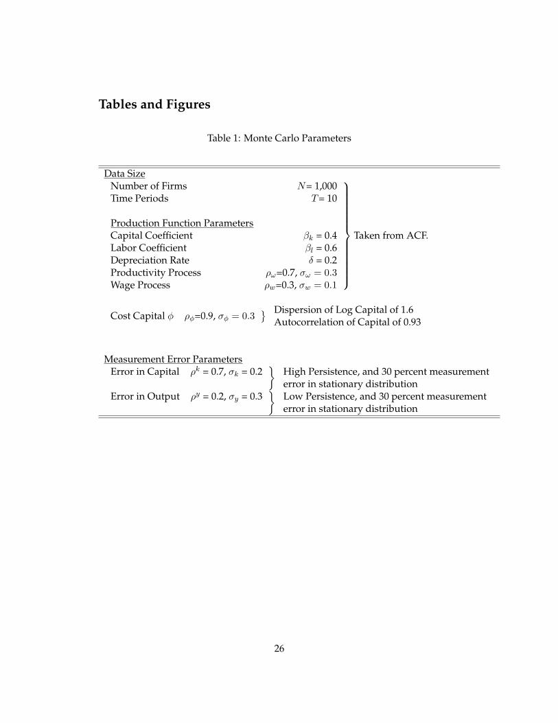
Table 1 shows the parameters used in our Monte Carlo. We pick the same pa-rameters for the size of the dataset, production function, and processes for pro-ductivity and wages as in ACF. For the process for the price of capital, denotedφit, we pick parameters that match the the cross-sectional dispersion of capital(std.[kit] = 1.6), and the time-series variation in capital (Corr.[kit − kit−1] = 0.93)in the Annual Survey of Industries in India (discussed in section 5), choosing anautocorrelation term for the process of φ of 0.9, and a shock variance of 0.3. In-deed, it is this last moment that the ACF monte carlo has difficulty replicating: itpredicts a serial correlation coefficient of capital of 0.997. Clearly this will makethe one-stage approach problematic, as both current and lagged capital are highlycollinear, much more so than in any producer level dataset we are aware of.

Finally, we pick parameters for the measurement error in inputs and outputs.We choose a measurement error for output with a standard deviation of 30 per-cent, and a low autocorrelation of 0.2. For capital, we choose a serial correlationcoefficient of 0.7, so a fairly high persistence, and a standard deviation of 0.2. Im-portantly, this assumption on the time series process for capital measurement erroryields a difference between k and k∗ which has a standard deviation of 30 percent.However, we precisely verify the sensitivity to the value of the capital measure-ment error’s standard deviation.

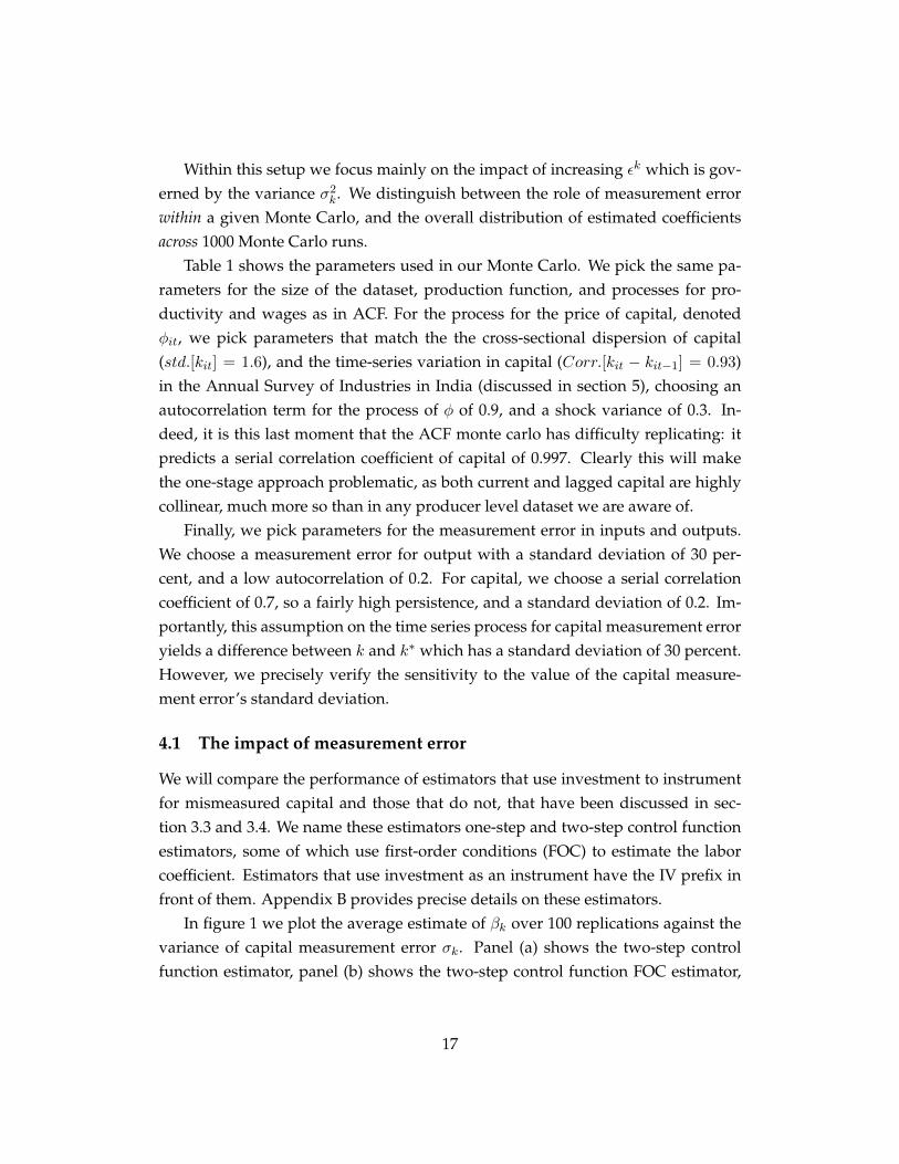
4.1 The impact of measurement error

We will compare the performance of estimators that use investment to instrumentfor mismeasured capital and those that do not, that have been discussed in sec-tion 3.3 and 3.4. We name these estimators one-step and two-step control functionestimators, some of which use first-order conditions (FOC) to estimate the laborcoefficient. Estimators that use investment as an instrument have the IV prefix infront of them. Appendix B provides precise details on these estimators.

In figure 1 we plot the average estimate of βk over 100 replications against thevariance of capital measurement error σk. Panel (a) shows the two-step controlfunction estimator, panel (b) shows the two-step control function FOC estimator,

17

and panel (c) shows the one-step control function estimator FOC.13

The first main result of our Monte Carlo simulations is that we find that stan-dard estimators, both the one-step FOC, two-step, and two-step FOC, become pro-gressively more biased as the measurement error in capital increases. It is of coursedifficult to guess the relevant range of this variance, but the main takeaway is thatour IV-based estimator is insulated from this problem. The simulations do suggestthat standard methods deliver an estimate of half the magnitude for a standarddeviation in the capital measurement error σk of about 0.2, which corresponds to astandard deviation between k and k∗ of 0.28 in the stationary distribution.

It is important to note that our estimators are robust to capital measurementerror, while still undoing the simultaneity bias that typically plagues the produc-tion function estimation. Therefore, applying our estimator when capital stock isaccurately measured provides consistent estimates of the production function co-efficients.

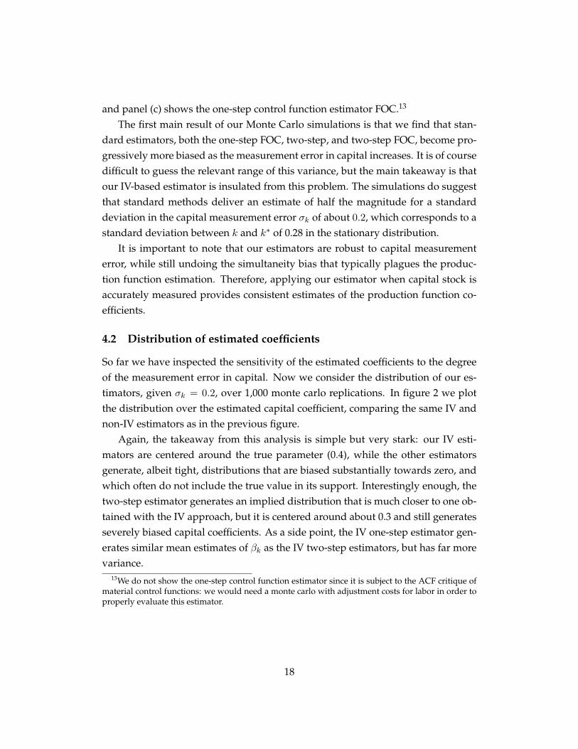
4.2 Distribution of estimated coefficients

So far we have inspected the sensitivity of the estimated coefficients to the degreeof the measurement error in capital. Now we consider the distribution of our es-timators, given σk = 0.2, over 1,000 monte carlo replications. In figure 2 we plotthe distribution over the estimated capital coefficient, comparing the same IV andnon-IV estimators as in the previous figure.

Again, the takeaway from this analysis is simple but very stark: our IV esti-mators are centered around the true parameter (0.4), while the other estimatorsgenerate, albeit tight, distributions that are biased substantially towards zero, andwhich often do not include the true value in its support. Interestingly enough, thetwo-step estimator generates an implied distribution that is much closer to one ob-tained with the IV approach, but it is centered around about 0.3 and still generatesseverely biased capital coefficients. As a side point, the IV one-step estimator gen-erates similar mean estimates of βk as the IV two-step estimators, but has far morevariance.

13We do not show the one-step control function estimator since it is subject to the ACF critique ofmaterial control functions: we would need a monte carlo with adjustment costs for labor in order toproperly evaluate this estimator.

18

4.3 Alternative sources of measurement error

As discussed before we have so far considered, what we refer to as, a reduced formfor the measurement error in capital. I.e. we consider the standard representationof an errors-in-variable, whereby the measurement error is (log) additive – herek + εk. In Appendix D we discuss an alternative source of measurement errorin capital, derived structurally from the measurement error in depreciation rates:Kit = (1 − δit)Kit−1 + Iit and δit = (δ + εdit); i.e., there is measurement error indepreciation rates.

This form of measurement error does not map into a log-additive structure, andwe therefore evaluate our estimator in the presence of this alternative setup. Themain takeaway from figure D.1 in the appendix is that our estimator outperformsthe other approaches (both in a one-step and two-step setting), but given the formalviolation of the moment conditions, leads to a small bias of the capital coefficientfor large values of the variance of the capital measurement error.

The evidence from the Monte Carlo unequivocally favors our estimator in thepresence of measurement error in capital, and moreover suggests that the bias canbe quite severe for moderate measurement error in capital. To verify how large thisproblem is in real data we now apply our estimator, exactly as performed in ourMonte Carlo analysis, to two different datasets of manufacturing plants, in Indiaand Slovenia.

5 Applications to plant-level data

We show our methodology in a couple of separate applications using plant-levelmicrodata. The first data that we use is the Annual Survey of Industries from India.This a plant-level survey for over 600,000 plants on a 20 year period. This datasethas been previously used and described in Allcott, Collard-Wexler, and O’Connell(2016). The second data set is the Slovenian Database, as used in De Loecker andWarzynski (2012) and De Loecker (2007) and covers all establishments in the Slove-nian manufacturing sector for the period 1994-2000. All variables are deflated us-ing industry-specific price deflators. Appendix A describes each dataset briefly,and presents basic summary statistics.

These two data sets have been used extensively to study productivity dynam-ics, but at the same time have distinct features related to the measurement of cap-ital. The data on Slovenian establishments reports the book value of plants and

19

investment, while the Indian census data reports both the book value and the (con-structed) capital stock using the perpetual inventory method. In addition, the eco-nomic environments are different in an important ways. There is substantial invest-ment during the process of economic transition in Slovenia, while in India, laborrepresents about 20 percent of value added, which is far below the cost share oflabor in most other countries. We expect these differences to materialize in the esti-mated coefficient, and the role and importance of measurement error in the capitalstock.

Throughout we will compare the production function coefficients obtained bysimple OLS, IV (without the simultaneity control), One-Step Control (i.e. the LPapproach), Two-Step Control (i.e. the ACF approach) and our approach, either IVOne-Step or IV Two-Step. We estimate a separate capital and labor coefficient foreach industry in both Slovenia and India.

We start by reporting the average labor and capital coefficients across the var-ious estimators in Table 2 below. We confirm a well known result in the literaturethat using fixed effects lowers the capital coefficient substantially, from an averageof 0.39 to 0.20 in India, and from 0.24 to 0.18 in Slovenia. By itself, this does notconclusively show that there is measurement error in capital. However, if capitalis fixed over a long period of time we can simply not identify its marginal productusing the time series variation within producers. Our next specification, IV (in-vestment), considers a two-stage least squares regression of output on capital andlabor, where we instrument for capital with investment. Thus, the IV estimatoralso ignores the simultaneity bias. We find substantially higher capital coefficientscompared to OLS, of 0.59 versus 0.39 in India, and 0.35 versus 0.24 in Slovenia. Thisreinforces our prior that instrumenting for capital with lagged investment may leadto a higher capital coefficient. In fact, the first-stage of this IV regression — a uni-variate regression of capital on lagged investment — has a R2 of 0.79 and 0.64 inSlovenia and India. However, investment and unobserved productivity are verylikely to be positively correlated, so the increase in the capital coefficient in the IVregression might be due to endogeneity problem as well.

The second panel lists the standard control function estimators used in the lit-erature; i.e. those that do not use investment as an instrument for capital, One-Stepand Two-Step Control, and also considers the FOC approach to estimating labor(denoted by FOC). They produce reasonable parameter estimates that are line withthe literature – i.e. capital coefficients of around 0.25.

20

The third panel lists the estimators based on our IV strategy, again for the one-step and two-step approach, and interacted with the FOC approach. We obtainmuch higher capital coefficients across both datasets and various specifications.For instance, the IV One-Step Control produces an average capital coefficient of0.41 and 0.41 for India and Slovenia, respectively, compared to 0.23 and 0.19 whenwe do not instrument the capital stock with lagged investment. Likewise, instru-menting with investment raises the Two-Step control estimate of capital from 0.31to 0.46 in India, and from 0.26 to 0.32 in Slovenia. More generally, the IV estimatorsproduce higher capital coefficient for all but one country-estimator pair.

These differences are not only statistically significant (at any level of signifi-cance), but most of all, are economically meaningful. The implied marginal prod-uct of capital and associated objects of interest, such as productivity dynamics arewidely different.

Our estimators also controls for the simultaneity of inputs, and this is reflectedin the labor coefficients: we find lower coefficients than obtained using OLS – againa standard finding in the literature. An attentive reader will also notice that theestimators that use first-order conditions give very different labor coefficients (witha smaller effect on capital coefficients). In particular, in India the labor coefficientfalls from 0.63 in the IV Two-Step Control, to 0.22 for the IV Two-Step Control FOC.Note that the labor coefficient in all the FOC methods is the same, since it is derivedfrom the input cost share of labor: in India, labor accounts for 22 percent of valueadded, versus 54 percent in Slovenia. Thus, the implausibly low labor coefficientsin India are not a result of our particular techniques. Instead, they suggest thatstatic labor choices are a particularly bad assumption in the Indian context.14

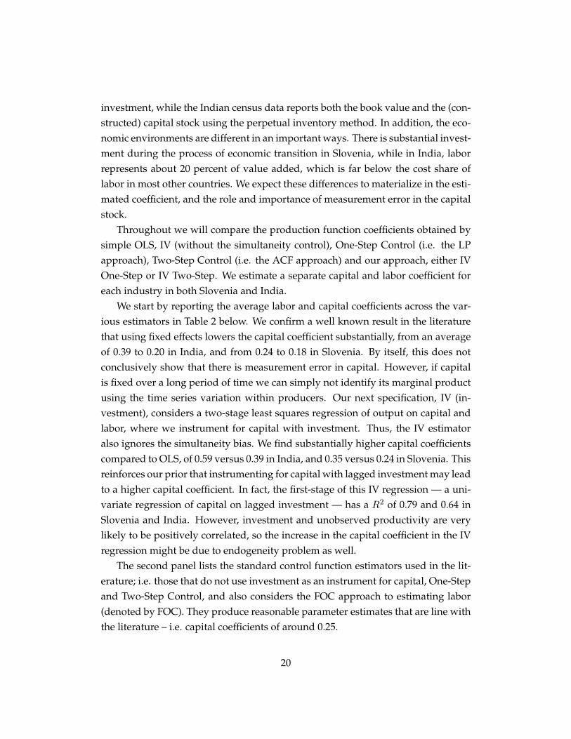
Finally, we plot the industry-specific capital coefficients by country in Figure 3,for our one-step and two-step estimators. For each panel, the left subpanel showsthe results for India, and the right subpanel shows the results for Slovenia. The ver-tical axis shows the capital coefficient from our IV estimator, while the horizontalaxis shows the capital coefficient that does not instrument with investment. Mostobservations are above the 45 degree line (in red), indicating that our IV estimatesare higher than the non-IV estimates for capital. On average we obtain capital co-efficients that are about two times larger, and this holds across all industries in allour data sets. If we go back to our Monte Carlo results, say in figure 1, dropping

14This is to be expected given the evidence on the prevalence of substantial labor adjustment costin the Indian labor market, which would invalidate the use of the FOC approach. See e.g. De Loecker,Goldberg, Khandelwal, and Pavcnik (2016) for a discussion.

21

the capital coefficient by half would indicate that the variance of the measurementerror σk is around 0.2.

This is very much in line with the results in Van Biesebroeck (2007), in partic-ular section V (ii) and Table II panel (4c) is relevant for our purpose: The reportedbias in the capital coefficient, between the estimated and the true value, is around−0.2 for the Olley and Pakes method, the most similar to our approach, and giventhe selected value for the capital coefficient of 0.4. Taking these results at face valuewould suggest that measurement error in capital could lead to obtain capital coef-ficients that are significantly lower – i.e. half the magnitude. This has importantconsequences for any subsequent productivity analysis, and we discuss this in thenext section.

6 Implications for productivity analysis

The results from the Monte Carlo and analysis of various census datasets points toa rather large bias in the capital coefficient. This biases our estimates of marginalproducts of capital, and propagate to productivity analysis as productivity esti-mates, such as measures of TFP, rely on estimates of the production function.

In what follows, we abstract away from the bias in the labor coefficient, andtherefore we can write the implied bias in the measured productivity residual ωm

as follows:ωmit = ωit + b · kit − βkεkit, (21)

where b measures the bias: b = (βk − βk).15 Our monte carlo exercises in section 4have shown that, without correcting for measurement error in capital, we shouldexpect βk < βk, and thus b > 0. This will lead to a spurious positive relationshipbetween productivity and size, if we measure size by the capital stock, of magni-tude b. Note that many of the outcomes that researchers have studied, such as therelationship between productivity and other important firm characteristics such asR&D activities or import and export behavior, may also suffer from bias in βk, tothe extent that these characteristics are correlated with capital stock — which theyare. This is precisely what we find both datasets.

15The last term βkεkit will not affect most of the analysis we are interested in here, as E(εkit) = 0.

22

Productivity dispersion

The dispersion of productivity has recently received tremendous amount of atten-tion, starting from earlier work by Syverson (2004), among others, and broughtto an cross-country context in the work of Hsieh and Klenow (2009). The latteridentified the mere presence of productivity dispersion as a potential diagnostic ofmisallocation of resources, and consequently an indication as to where to look fordrivers of difference in income across countries.

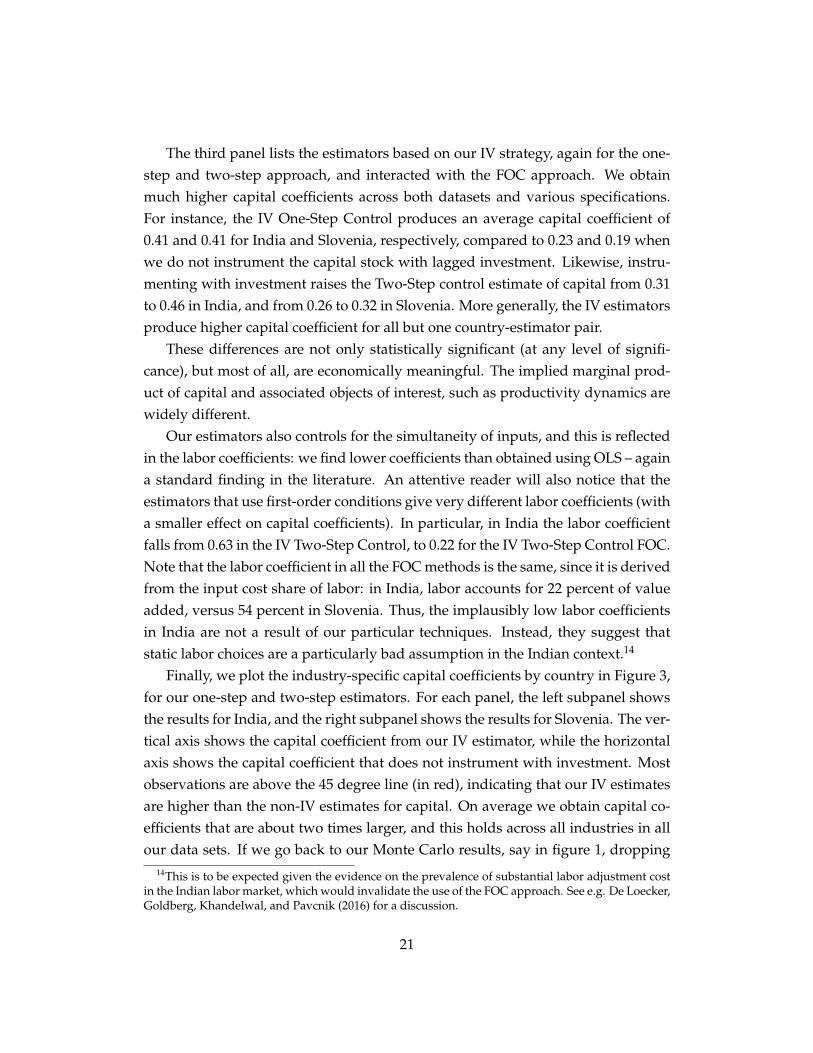
It is easy to show that the dispersion of productivity, which is typically mea-sured using the standard deviation of log productivity (Std.(ω)), is again a func-tion of the bias in our estimate of βk. Indeed, the difference between the standarddeviation of productivity, with and without measurement . term and therefore willalso depend on the variance of the capital stock and the covariance of capital andoutput. The difference between the variance with and without the bias in βk isgiven by: b · var(k) + 2b · cov(y, k), and therefore we can expect to find a larger dis-persion of TFPR, which would then suggest for example a (potential) larger degreeof misallocation.

To highlight the possibility of such a finding, in Figure 4 we plot the distributionof the corrected and uncorrected (ACF based) productivity for the entire Indianmanufacturing dataset. We confirm that the mean of productivity is higher, andthat the standard deviation of productivity is also higher.

7 Conclusion

This paper revisits the estimation of production functions, using standard data onoutput and inputs, in the presence of measurement error in inputs, and in capital inparticular. Our starting point is that appropriately measuring capital is one of themost difficult tasks that go into estimating a production function. There is, how-ever, rather surprisingly little work that directly deals with the potential presenceof measurement error in capital, or any input for that matter.

We introduce an estimator that relies on a hybrid IV-control function approach,and we build on what have now become standard techniques to address the si-multaneity bias, and add an IV strategy to correct for the measurement error ofcapital. We propose a simple strategy that relies on investment to inform us aboutthe marginal product of capital; and specifically we use investment as an instru-ment for the capital stock while still controlling for the standard simultaneity bias.

23

Investment is an instrument and therefore an excluded variable from the controlfunction.

Monte Carlo simulations show that our estimator performs well even in cases ofrather large measurement error. We also apply our estimator to Indian and Slove-nian census data. We find capital coefficients that are about twofold of those ob-tained with standard techniques. These results suggest that correcting for measure-ment error in capital can be a first order concern, and it has immediate implicationsfor the literature that studies productivity dynamics, firm growth, investment, andthe covariates of productivity growth, to name but a few.

References

ACKERBERG, D., G. FRAZER, AND K. CAVES (2015): “Identification Properties ofRecent Production Function Estimators,” Econometrica, forthcoming.

ALLCOTT, H., A. COLLARD-WEXLER, AND S. D. O’CONNELL (2016): “How DoElectricity Shortages Affect Industry? Evidence from India,” American EconomicReview, 106(3), 587–624.

BECKER, R. A., AND J. HALTIWANGER (2006): “Micro and macro data integration:The case of capital,” in A new architecture for the US national accounts, pp. 541–610.University of Chicago Press.

BOND, S., AND M. SODERBOM (2005): “Adjustment costs and the identificationof Cobb Douglas production functions,” Discussion paper, IFS Working Papers,Institute for Fiscal Studies (IFS).

DE LOECKER, J. (2007): “Do Exports Generate Higher Productivity? Evidence fromSlovenia,” Journal of International Economics, (73), 69–98.

DE LOECKER, J., P. GOLDBERG, A. KHANDELWAL, AND N. PAVCNIK (2016):“Prices, Markups and Trade Reform,” Econometrica, 84(2), 445–510.

DE LOECKER, J., AND F. WARZYNSKI (2012): “Markups and firm-level export sta-tus,” American Economic Review, 102(6), 2437–2471.

GRILICHES, Z., AND J. MAIRESSE (1998): Production Functions: The Search for Identi-ficationpp. 169–203. Cambridge University Press.

24

HAUSMAN, J. A., W. K. NEWEY, H. ICHIMURA, AND J. L. POWELL (1991): “Iden-tification and estimation of polynomial errors-in-variables models,” Journal ofEconometrics, 50(3), 273–295.

HICKS, J. R. (1981): Wealth and Welfare: Collected Essays on Economic Theory, vol. 1.Oxford: Blackwell.

HSIEH, C.-T., AND P. J. KLENOW (2009): “Misallocation and Manufacturing TFP inChina and India,” Quarterly Journal of Economics, 124(4), 1403–1448.

HU, Y., AND M. SHUM (2013): “Identifying dynamic games with serially-correlatedunobservables,” Advances in Econometrics, 31, 97–113.

KIM, K., A. PETRIN, AND S. SONG (2016): “Estimating production functions withcontrol functions when capital is measured with error,” Journal of Econometrics,190(2), 267–279.

LEVINSOHN, J., AND A. PETRIN (2003): “Estimating Production Functions UsingInputs to Control for Unobservables,” Review of Economic Studies, 70(2), 317–341.

OLLEY, G. S., AND A. PAKES (1996): “The dynamics of productivity in the telecom-munications equipment industry,” Econometrica, 64(6), 35.

PROGRESS ENERGY – CAROLINAS (2010): “Electricity Utility Plant DepreciationRate Study,” Docket E-2 Sub 1025.

SCHENNACH, S. M. (2004): “Estimation of nonlinear models with measurementerror,” Econometrica, pp. 33–75.

SYVERSON, C. (2001): “Output Market Segmentation, Heterogeneity, and Produc-tivity,” Ph.D. thesis, University of Maryland.

(2004): “Market Structure and Productivity: A Concrete Example,” Journalof Political Economy, 112(6), 1181–1222.

VAN BIESEBROECK, J. (2007): “Robustness of Productivity Estimates,” Journal ofIndustrial Economics, 3(55), 529–539.

WOOLDRIDGE, J. M. (2009): “On estimating firm-level production functions usingproxy variables to control for unobservables,” Economics Letters, 104(3), 112–114.

25

Tables and Figures

Table 1: Monte Carlo Parameters

Data SizeNumber of Firms N= 1,000Time Periods T= 10

Production Function ParametersCapital Coefficient βk = 0.4Labor Coefficient βl = 0.6Depreciation Rate δ = 0.2Productivity Process ρω=0.7, σω = 0.3Wage Process ρw=0.3, σw = 0.1

Taken from ACF.

Cost Capital φ ρφ=0.9, σφ = 0.3 Dispersion of Log Capital of 1.6

Autocorrelation of Capital of 0.93

Measurement Error ParametersError in Capital ρk = 0.7, σk = 0.2

High Persistence, and 30 percent measurementerror in stationary distribution

Error in Output ρy = 0.2, σy = 0.3

Low Persistence, and 30 percent measurementerror in stationary distribution

26

Table 2: Mean Industry-Level Coefficients

India Slovenia(Nr Ind. =19) (Nr Ind. =18)

Capital Labor Capital LaborOLS 0.39 0.78 0.24 0.83FE 0.20 0.59 0.18 0.77IV (investment) 0.59 0.51 0.35 0.70

One-Step Control 0.23 0.41 0.19 0.65Two-Step Control 0.31 0.91 0.26 0.47Two-Step Control (Adj) 0.36 0.71 0.21 0.85One-Step Control, Labor FOC 0.25 0.22 0.20 0.54Two-Step Control, Labor FOC 0.57 0.22 0.42 0.54

IV One-Step Control 0.41 0.37 0.41 0.61IV Two-Step Control 0.46 0.63 0.32 0.67IV Two-Step Control (Adj) 0.56 0.53 0.32 0.74IV One-Step Control, Labor FOC 0.47 0.22 0.44 0.54IV Two-Step Control, Labor FOC 0.68 0.22 0.40 0.54

Notes: We report the average capital across all industries for each dataset. We consider value-addedbased Cobb-Douglas production functions with material demand as a control for productivity, andan AR(1) process for productivity. FOC refers to case where the labor coefficient is obtained usingthe FOC approach – i.e. we compute the median of the wage bill to sales ratio for each industryseparately. All estimators labeled with FOC thus have the same estimate for labor – i.e. the medianof the wage bill over sales, by industry. (Adj) refers to the specification with both labor and capitaladjustment costs – i.e. current labor is used as the instrument.

27

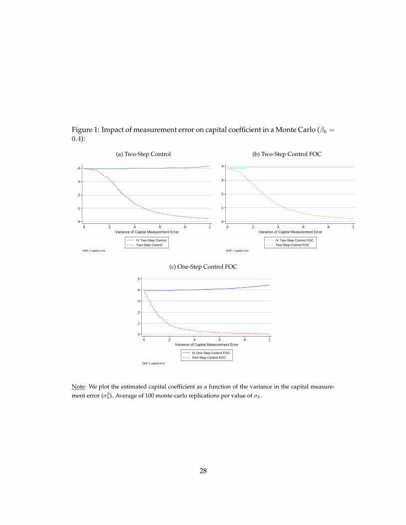
Figure 1: Impact of measurement error on capital coefficient in a Monte Carlo (βk =0.4):

(a) Two-Step Control

0

.1

.2

.3

.4

0 .2 .4 .6 .8 1

Variance of Capital Measurement Error

IV Two-Step ControlTwo-Step Control

DGP 1 capital error

(b) Two-Step Control FOC

0

.1

.2

.3

.4

0 .2 .4 .6 .8 1

Variance of Capital Measurement Error

IV Two-Step Control FOCTwo-Step Control FOC

DGP 1 capital error

(c) One-Step Control FOC

0

.1

.2

.3

.4

.5

0 .2 .4 .6 .8 1

Variance of Capital Measurement Error

IV One-Step Control FOCOne-Step Control FOC

DGP 1 capital error

Note: We plot the estimated capital coefficient as a function of the variance in the capital measure-ment error (σ2

k). Average of 100 monte-carlo replications per value of σk.

28

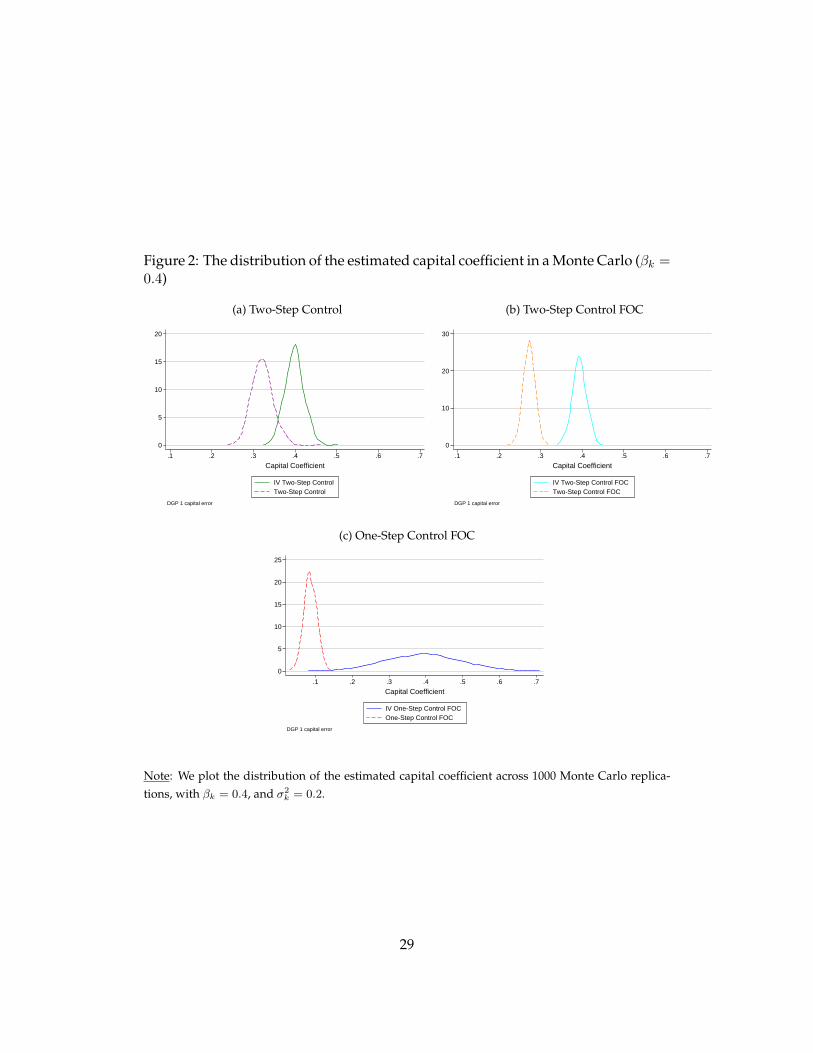
Figure 2: The distribution of the estimated capital coefficient in a Monte Carlo (βk =0.4)

(a) Two-Step Control

0

5

10

15

20

.1 .2 .3 .4 .5 .6 .7

Capital Coefficient

IV Two-Step ControlTwo-Step Control

DGP 1 capital error

(b) Two-Step Control FOC

0

10

20

30

.1 .2 .3 .4 .5 .6 .7

Capital Coefficient

IV Two-Step Control FOCTwo-Step Control FOC

DGP 1 capital error

(c) One-Step Control FOC

0

5

10

15

20

25

.1 .2 .3 .4 .5 .6 .7

Capital Coefficient

IV One-Step Control FOCOne-Step Control FOC

DGP 1 capital error

Note: We plot the distribution of the estimated capital coefficient across 1000 Monte Carlo replica-tions, with βk = 0.4, and σ2

k = 0.2.

29

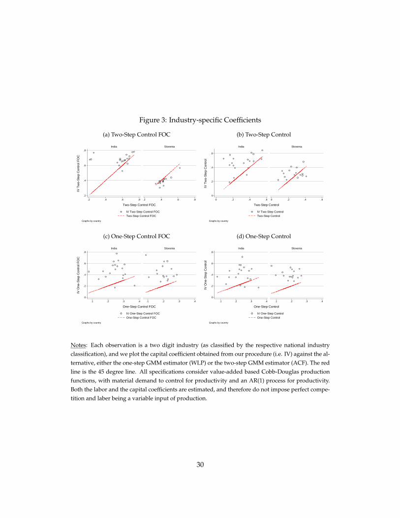
Figure 3: Industry-specific Coefficients

(a) Two-Step Control FOC

.2

.4

.6

.8

.2 .4 .6 .8 .2 .4 .6 .8

India Slovenia

IV Two-Step Control FOCTwo-Step Control FOC

IV T

wo-

Ste

p C

ontr

ol F

OC

Two-Step Control FOC

Graphs by country

(b) Two-Step Control

0

.2

.4

.6

0 .2 .4 .6 0 .2 .4 .6

India Slovenia

IV Two-Step ControlTwo-Step Control

IV T

wo-

Ste

p C

ontr

olTwo-Step Control

Graphs by country

(c) One-Step Control FOC

0

.2

.4

.6

.8

.1 .2 .3 .4 .1 .2 .3 .4

India Slovenia

IV One-Step Control FOCOne-Step Control FOC

IV O

ne-S

tep

Con

trol

FO

C

One-Step Control FOC

Graphs by country

(d) One-Step Control

0

.2

.4

.6

.8

.1 .2 .3 .4 .1 .2 .3 .4

India Slovenia

IV One-Step ControlOne-Step Control

IV O

ne-S

tep

Con

trol

One-Step Control

Graphs by country

Notes: Each observation is a two digit industry (as classified by the respective national industryclassification), and we plot the capital coefficient obtained from our procedure (i.e. IV) against the al-ternative, either the one-step GMM estimator (WLP) or the two-step GMM estimator (ACF). The redline is the 45 degree line. All specifications consider value-added based Cobb-Douglas productionfunctions, with material demand to control for productivity and an AR(1) process for productivity.Both the labor and the capital coefficients are estimated, and therefore do not impose perfect compe-tition and laber being a variable input of production.

30

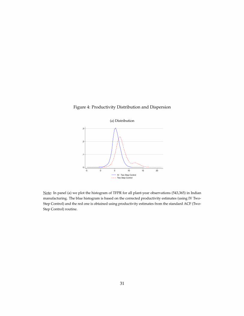
Figure 4: Productivity Distribution and Dispersion

(a) Distribution

0

.1

.2

.3

-5 0 5 10 15 20

IV - Two Step ControlTwo Step Control

Note: In panel (a) we plot the histogram of TFPR for all plant-year observations (543,365) in Indianmanufacturing. The blue histogram is based on the corrected productivity estimates (using IV Two-Step Control) and the red one is obtained using productivity estimates from the standard ACF (Two-Step Control) routine.

31

A Data Appendix

We apply our estimator to two datasets, covering manufacturing plants in India and Slove-nia. There have been numerous productivity studies using these data, and therefore arecompletely standard in which variables are reported, and how they are constructed.

A.1 Slovenian manufacturing

We refer the reader to De Loecker (2007) for a detailed discussion of the data. For thissetting it is important to note that the data contain standard information on establishment-level production and that similar data have been used throughout the literature. See, forexample Olley and Pakes (1996) and Levinsohn and Petrin (2003).

In particular, and as mentioned in the paper, the data represent the population of pro-ducers of manufacturing products over the period 1994-2000. The estimation of the pro-duction function requires information on plant-level output (revenues deflated with de-tailed producer price indices), (deflated) value added, and input use: labor as measuredby full-time equivalent production workers, raw materials and a measure of the capitalstock. The latter is constructed from the balance sheet information on total fixed assetsbroken down into 1) machinery and equipment, 2) land and buildings and 3) furniture andvehicles. Appropriate depreciation rates (based on actual depreciation rates) are used toconstruct a firm-level capital stock series using standard techniques. See, for example, thedata appendix in Olley and Pakes (1996).

In addition, the data report investment and provide detailed information on owner-ship, firm entry and exit. Finally, the export status and export revenues – at every pointin time – provide information whether a firm is a domestic producer, an export entrantor a continuing exporter. This gives rise to an unbalanced panel of about six thousandproducers, covering the period 1994-2000.

A.2 Indian manufacturing

We use India’s Annual Survey of Industries (ASI) for establishment-level microdata, andthis dataset is described in more detail in Allcott, Collard-Wexler, and O’Connell (2016).Registered factories with over 100 workers (the “census scheme”) are surveyed every year,while smaller establishments (the “sample scheme”) are typically surveyed every three tofive years. The publicly available ASI includes establishment identifiers that are consistentacross years beginning in 1998, but we have plant identifiers going back to 1992. We havea plant-level panel for the entire 1992-2010 sample.

The ASI is comparable to manufacturing surveys in the United States and other coun-tries. Variables include revenues, value of fixed capital stock, total workers employed, totalcosts of labor, and materials. Industries are grouped using India’s NIC (National IndustrialClassification) codes, which are closely related to SIC (Standard Industrial Classification)codes.

There are 615,721 plant-by-year observations at 224,684 unique plants. 107,032 plantswill be immediately dropped from our estimators because they are observed only once.For plants observed multiple times, 60 percent of intervals between observations are oneyear, while 91 percent are five years or less.

The mean (median) plant employs 79 (34) people and has gross revenues of 139 million(20 million) Rupees, or in U.S. dollars approximately $3 million ($400,000).

32

B Estimators: Details

In this section we describe the estimators proposed in this paper in great detail, enoughso that these estimator can easily be coded up by other researchers, and code for theseestimators is also available in STATA. In what follows, we use materials as the static controlfunction decision d∗.

B.1 One-Step Estimators, Labor FOC

1. Estimate βl

βl = Median

(WLitPYit

).

2. Produce output yit netted out from labor contribution.

yit = yit − βllit

3. Estimateyit = βkkit + θkkit−1 + θllit−1 + θddit−1 + εit

using instruments xit = [iit−1, iit−2, lit−1, dit−1]

Notice that we refer to the non-IV version of this estimator as the estimator that esti-mates yit = βkkit + θkkit−1 + θllit−1 + θddit−1 by OLS.

B.2 One-Step Estimators, Labor Adjustment Costs

Estimate:yit = βllit + βkkit + θkkit−1 + θllit−1 + θddit−1

by two-stage least-squares using instruments xit = [lit, iit−1, iit−2, lit−1, dit−1]. Notice thatwe refer to the non-IV version of this estimator as the estimator that estimates this previousequation by OLS.

B.3 Two-Step Estimators, Labor FOC

1. Estimate βl

βl = Median

(WLitPYit

).

2. Produce output yit netted out from labor contribution.

yit = yit − βllit

3. Estimate

yit = θddit

by OLS, and obtain yit = θddit.

33

4. For a parameter βk, minimize the criterion Q(βk) using:

(a) Compute ωit = yit − βkkit(b) Estimate the AR(1) process for productivity, ωit = ρωit−1 , by OLS, obtain ρ.

Recover productivity shock ξit = ωit − ρωit−1.

(c) ComputeQ(βk) as the empirical analogue of the moment condition E[ξitiit−1] =0.

Q(βk) = (ξz)′(z′z)−1(ξz)

where ξ denotes the stacked vector of ξit, and z denotes the stacked vector ofiit−1.

(d) Find βk as the minimizer of Q(βk).

B.4 Two-Step Estimators, Labor Adjustment Costs

1. Estimate the regression:yit = θddit,

by OLS.

Obtain yit = θddit.

2. For a parameter β = [βk, βl], minimize the criterion Q(β) using:

(a) Compute ωit = yit − βkkit − βllit(b) Estimate the AR(1) process for productivity, ωit = ρωit−1 , by OLS, obtain ρ.

Recover productivity shock ξit = ωit − ρωit−1.

(c) ComputeQ(β) as the empirical analogue of the moment condition E[ξit

(litiit−1

)] =

0 given by:Q(β) = (ξZ)′(Z ′Z)−1(ξZ) (B.1)

where ξ denotes the stacked vector of ξit, and Z denotes the stacked matrix ofxit = [lit, iit−1].

(d) Compute βk as the minimizer of Q(βk).

34

C Monte Carlo

In this section, we describe details of the Monte-Carlo that we will use to evaluate the per-formance of our estimator. We will need to specify laws of motion for each of the variablesin the data generating process.

C.1 Timing

First, we specify the timing assumptions in our model. Investment is chosen with one pe-riod time to build. Materials are chosen statically, i.e., after the firm knows it’s productivityΩit. Labor is chosen statistically in for DGP 2 and DGP 3, and in an interim period for DGP1, i.e. part of the productivity shock is revealed before the firm makes its labor choice.

Second, there are three exogenous state variables, productivity Ait, wages Wit, out-put prices Pit, and the price of capital φit, which all have log AR(1) processes. The onlyendogenous state variable is capital.

Logged productivity A has a first-order Markov evolution:

ait = ρaait−1 + uait, (C.1)

where ua ∼ N (0, σ2a).

As well, log wages have a first-order markov process:

wit = ρwwit−1 + uwit, (C.2)

and likewise for the logged price for output (P ):

pit = ρppit−1 + upit. (C.3)

where uw ∼ N (0, σ2w) and up ∼ N (0, σ2

p). For the purposes of the Monte-Carlo, we willnormalize pit ≡ 1, the case of perfect competition.

C.2 Derivation of Investment Policy as in Syverson (2001)

In this section, we derive a closed form for the investment function in Syverson (2001), toshow that we can allow a time varying cost of capital φit. This derivation is very close toSyverson (2001), so our goal is merely to show that this model admits a time-varying costof capital φit.

Firms have flow profits given by:

Πit = PitAitLαitK

1−αit −WitLit −

φit2I2it, (C.4)

where P is the price of output, A is physical productivity, W refers to firm specificwages, and I is investment.

The firm’s value function V is given by:

V (Pit, Ait,Kit,Wit, φit) = maxLit,Kit

PitAitLαitK

1−αit −WitLit

+ βEitV (Pit+1, Ait+1,Kit+1,Wit+1, φit+1)

such that Kit+1 = (1− δ)Kit + Iit

(C.5)

35

where δ is the depreciation rate of capital.Labor is chosen using the usual first-order condition ∂Πit

∂Lit= 0:

PitAitαLα−1it K1−α

it = Wit

→ Lit =

[αPitAitWit

] 11−α

Kit

(C.6)

And likewise, investment solves the Euler Equation, ∂V∂I = 0 giving,

φitIit = βEitVK(Pit+1, Ait+1,Kit+1,Wit+1, φit+1). (C.7)

The envelope condition yields:

VK(Pit, Ait,Kit,Wit, φit) =(1− α)PitAitLαitK−αit

+ (1− δ)EitVK(Pit+1, Ait+1,Kit+1,Wit+1, φit+1)(C.8)

Substituting into the first-order conditions, the envelope condition becomes

φitIit =βEit[(1− α)α

α1−αW

− α1−α

it+1 P1

1−αit+1A

11−αit+1

]+ β(1− δ)Eitφit+1Iit+1 (C.9)

And then iterating this equation forward; i.e., replacing EitφitIit with the right handside in equation (C.9), yields:

φitIit =βEit[(1− α)α

α1−αW

− α1−α

it+1 P1

1−αit+1A

11−αit+1

]+ β(1− δ)Eitβ

[(1− α)α

α1−αW

− α1−α

it+2 P1

1−αit+2A

11−αit+2

]+ [β(1− δ)]2 Et+1φit+2Iit+2

φitIit =βEit[(1− α)α

α1−αW

− α1−α

it+1 P1

1−αit+1A

11−αit+1

]+ β(1− δ)Eitβ

[(1− α)α

α1−αW

− α1−α

it+2 P1

1−αit+2A

11−αit+2

]+ [β(1− δ)]2 β

[(1− α)α

α1−αW

− α1−α

it+3 P1

1−αit+3A

11−αit+3

]+ [β(1− δ)]3 Et+2φit+3Iit+3.

(C.10)

Writing in the form of geometric series

Iit =β(1− α)

φitα

α1−αEit

∞∑j=0

[β(1− δ)]jW−

α1−α

it+1+jP1

1−αit+1+jA

11−αit+1+j

(C.11)

Given that we have assume that Pit, Ait and Wit follow the log-linear AR(1) processwith normal error terms:

36

then the investment function becomes

Iit =β(1− α)

φitα

α1−αEit

∞∑j=0

[β(1− δ)]jW−αφi+1w

1−αit

j∏s=0

(uwt+1+i−s)−αφ

sw

1−α Pφi+1p

1−αit

·j∏s=0

(upt+1+i−s)φsp1−αA

φi+1a

1−αit

j∏s=0

(uat+1+i−s)φsa1−α

=β(1− α)

φitα

α1−α

j∏s=0

[β(1− δ)]jW−αφi+1w

1−αit

j∏s=0

Eit(uwt+1+i−s)−αφ

sw

1−α Pφi+1p

1−αit

·j∏s=0

Eit[(upt+1+i−s)φsp1−α ]A

φi+1a

1−αit

j∏s=0

Eit[(uat+1+i−s)φsa1−α ]

Since for ε ∼ N (0, σ2), we have E(uφs

1−α ) = exp( σ2φ2s

2(1−α)2 ), then the investment functioncan be further simplified as:

Iit =β(1− α)

φitα

α1−αEit

∞∑i=0

[β(1− δ)]jW−αφi+1w

1−αit

j∏s=0

exp

(α2σ2

wφ2sw

2(1− α)2

)Pφi+1p

1−αit

·j∏s=0

exp

(σ2pφ

2sp

2(1− α)2

)Aφi+1a

1−αit

j∏s=0

exp

(σ2aφ

2sa

2(1− α)2

).

(C.12)

C.3 Process for the Price of Capital

In the original Monte-Carlo proposed by Ackerberg, Frazer, and Caves (2015), the authorsextend the model proposed by Syverson (2001) by allowing for the price for capital φ todiffer between firms, i.e. to allow the price for capital to be a firm specific φi. This is impor-tant, in the context of their Monte-Carlo, since it allows a higher cross-sectional dispersionof capital between firms than what is generated by reasonable processes of productivity,given the patterns in standard producer-level data.

In this paper, we also need capital to move around more than what would be generatedby the process considered by Ackerberg, Frazer, and Caves (2015), which generates a serialcorrelation coefficient for capital of 0.99. Instead, we have the following AR(1) process:

φit = ρφφit−1 + σφuφit, (C.13)

where uφit ∼ N (0, 1).Figure C.1 shows the relationship between the autocorrelation of the price of capital

and estimates of the capital coefficient using both the one and two step estimators proposedin the paper. To make these estimates more comparable, when we change ρφ, we adjust σφ

so that the stationary distribution of φ, given by the usual formula for an AR(1) processwith normal errors σ√

1−ρ2, is unchanged. In panel a, showing one-step estimators, for a

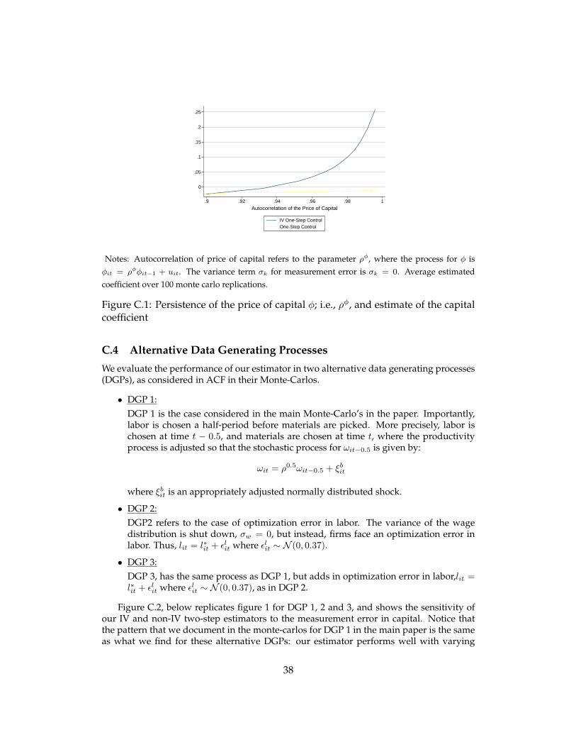
wide range range of ρφ parameters below one, our estimator performs very well. However,at very high levels of persistence of φ, our IV one-step estimate drop to 0.2. In contrast, theestimates for panel b showing two-step estimators, do not change much as we vary thepersistence of the price of capital φ.

37

0

.05

.1

.15

.2

.25

.9 .92 .94 .96 .98 1

Autocorrelation of the Price of Capital

IV One-Step ControlOne-Step Control

Notes: Autocorrelation of price of capital refers to the parameter ρφ, where the process for φ isφit = ρφφit−1 + uit. The variance term σk for measurement error is σk = 0. Average estimatedcoefficient over 100 monte carlo replications.

Figure C.1: Persistence of the price of capital φ; i.e., ρφ, and estimate of the capitalcoefficient

C.4 Alternative Data Generating Processes

We evaluate the performance of our estimator in two alternative data generating processes(DGPs), as considered in ACF in their Monte-Carlos.

• DGP 1:DGP 1 is the case considered in the main Monte-Carlo’s in the paper. Importantly,labor is chosen a half-period before materials are picked. More precisely, labor ischosen at time t − 0.5, and materials are chosen at time t, where the productivityprocess is adjusted so that the stochastic process for ωit−0.5 is given by:

ωit = ρ0.5ωit−0.5 + ξbit

where ξbit is an appropriately adjusted normally distributed shock.

• DGP 2:DGP2 refers to the case of optimization error in labor. The variance of the wagedistribution is shut down, σw = 0, but instead, firms face an optimization error inlabor. Thus, lit = l∗it + εlit where εlit ∼ N (0, 0.37).

• DGP 3:DGP 3, has the same process as DGP 1, but adds in optimization error in labor,lit =l∗it + εlit where εlit ∼ N (0, 0.37), as in DGP 2.

Figure C.2, below replicates figure 1 for DGP 1, 2 and 3, and shows the sensitivity ofour IV and non-IV two-step estimators to the measurement error in capital. Notice thatthe pattern that we document in the monte-carlos for DGP 1 in the main paper is the sameas what we find for these alternative DGPs: our estimator performs well with varying

38

degrees of capital measurement error, while the standard control function approaches arebiased for reasonable amounts of measurement error.

39

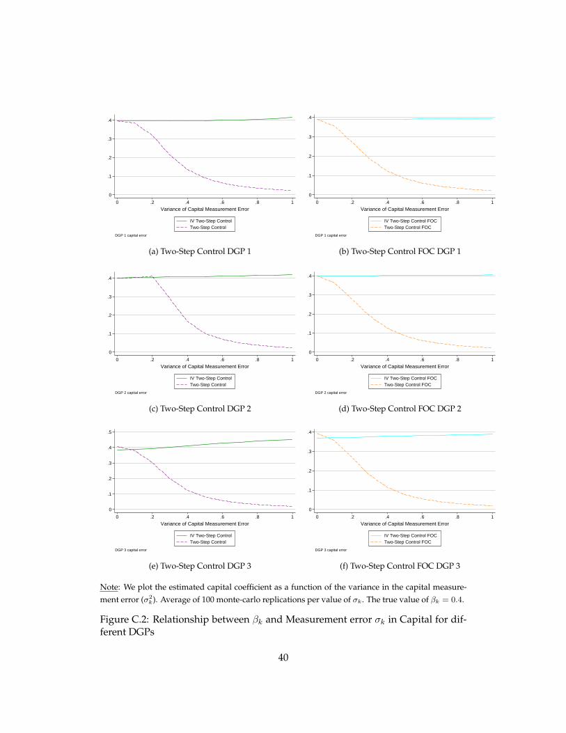
0

.1

.2

.3

.4

0 .2 .4 .6 .8 1

Variance of Capital Measurement Error

IV Two-Step ControlTwo-Step Control

DGP 1 capital error

(a) Two-Step Control DGP 1

0

.1

.2

.3

.4

0 .2 .4 .6 .8 1

Variance of Capital Measurement Error

IV Two-Step Control FOCTwo-Step Control FOC

DGP 1 capital error

(b) Two-Step Control FOC DGP 1

0

.1

.2

.3

.4

0 .2 .4 .6 .8 1

Variance of Capital Measurement Error

IV Two-Step ControlTwo-Step Control

DGP 2 capital error

(c) Two-Step Control DGP 2

0

.1

.2

.3

.4

0 .2 .4 .6 .8 1

Variance of Capital Measurement Error

IV Two-Step Control FOCTwo-Step Control FOC

DGP 2 capital error

(d) Two-Step Control FOC DGP 2

0

.1

.2

.3

.4

.5

0 .2 .4 .6 .8 1

Variance of Capital Measurement Error

IV Two-Step ControlTwo-Step Control

DGP 3 capital error

(e) Two-Step Control DGP 3

0

.1

.2

.3

.4

0 .2 .4 .6 .8 1

Variance of Capital Measurement Error

IV Two-Step Control FOCTwo-Step Control FOC

DGP 3 capital error

(f) Two-Step Control FOC DGP 3

Note: We plot the estimated capital coefficient as a function of the variance in the capital measure-ment error (σ2

k). Average of 100 monte-carlo replications per value of σk. The true value of βk = 0.4.

Figure C.2: Relationship between βk and Measurement error σk in Capital for dif-ferent DGPs

40

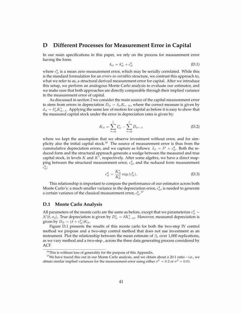
D Different Processes for Measurement Error in Capital

In our main specifications in this paper, we rely on the process for measurement errorhaving the form:

kit = k∗it + εkit (D.1)

where εkit is a mean zero measurement error, which may be serially correlated. While thisis the standard formulation for an errors-in-variables structure, we contrast this approach to,what we refer to as, a structural derived measurement error for capital. After we introducethis setup, we perform an analogous Monte Carlo analysis to evaluate our estimator, andwe make sure that both approaches are directly comparable through their implied variancein the measurement error of capital.

As discussed in section 2 we consider the main source of the capital measurement errorto stem from errors in depreciation Dit = δitKi−1t, where the correct measure is given bydit = δ∗itK

∗it−1. Applying the same law of motion for capital as before it is easy to show that

the measured capital stock under the error in depreciation rates is given by:

Kit =

t∑τ=0

I∗iτ −t∑

τ=0

Diτ−1 (D.2)

where we kept the assumption that we observe investment without error, and for sim-plicity also the initial capital stock.16 The source of measurement error is thus from thecummulative depreciation errors, and we capture as follows: δit = δ∗ + εdit. Both the re-duced form and the structural approach generate a wedge between the measured and truecapital stock, in levels K and K∗, respectively. After some algebra, we have a direct map-ping between the structural measurement error, εdit, and the reduced form measurementεkit:

εdit =K∗itK∗0

exp (εkit). (D.3)

This relationship is important to compare the performance of our estimator across bothMonte Carlo’s: a much smaller variance in the depreciation error, εdit, is needed to generatea certain variance of the classical measurement error, εkit.

17

D.1 Monte Carlo Analysis

All parameters of the monte carlo are the same as before, except that we parameterize εdit ∼N (0, σd). True depreciation is given by D∗it = δK∗i−1t. However, measured depreciation isgiven by Dit = (δ + εdit)Kit.

Figure D.1 presents the results of this monte carlo for both the two-step IV controlmethod we propose and a two-step control method that does not use investment as aninstrument. Plot the relationship between the mean estimate of βk over 1,000 replications,as we vary method and a two-step , across the three data generating process considered byACF.

16This is without loss of generality for the purpose of this Appendix.17We have traced this out in our Monte Carlo analysis, and we obtain about a 20-1 ratio – i.e., we

obtain similar implied variances for the measurement error using either σk = 0.2 or σd = 0.01.

41

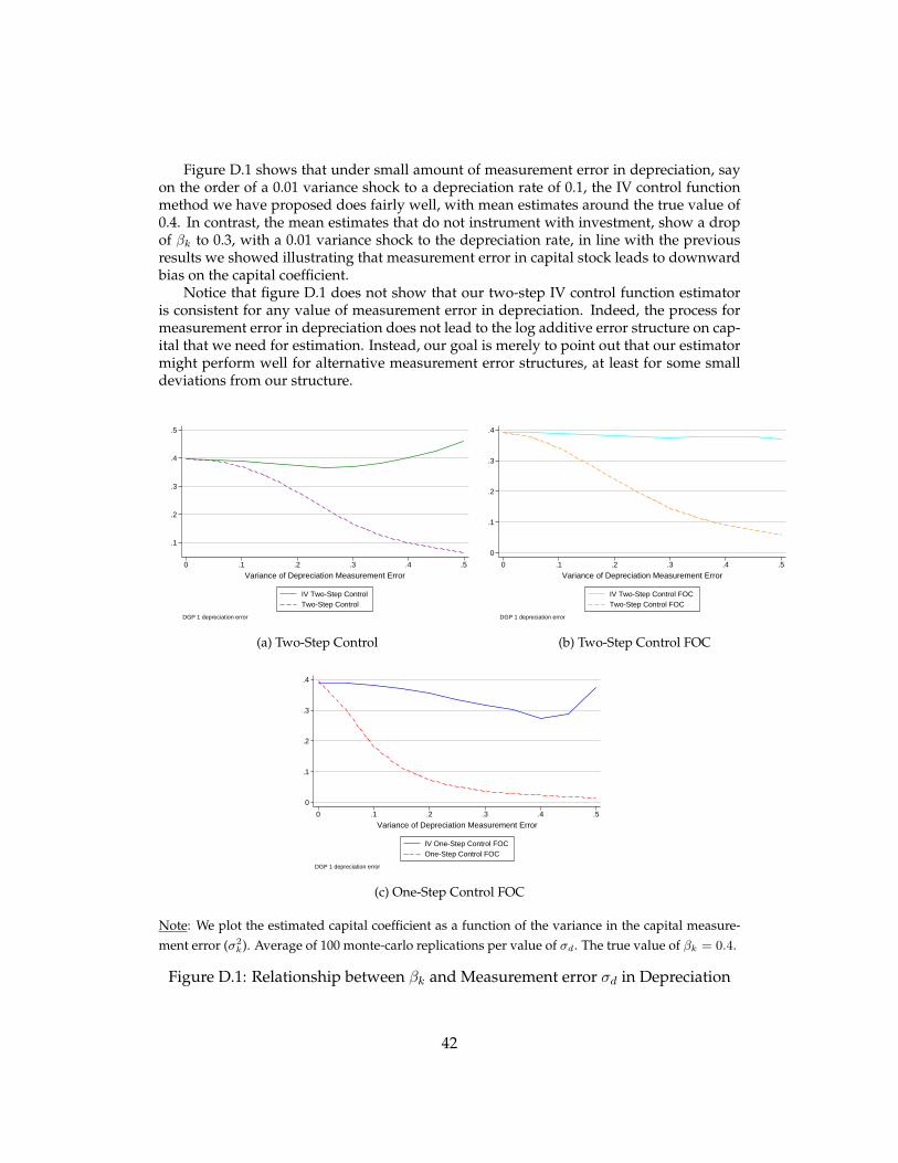
Figure D.1 shows that under small amount of measurement error in depreciation, sayon the order of a 0.01 variance shock to a depreciation rate of 0.1, the IV control functionmethod we have proposed does fairly well, with mean estimates around the true value of0.4. In contrast, the mean estimates that do not instrument with investment, show a dropof βk to 0.3, with a 0.01 variance shock to the depreciation rate, in line with the previousresults we showed illustrating that measurement error in capital stock leads to downwardbias on the capital coefficient.

Notice that figure D.1 does not show that our two-step IV control function estimatoris consistent for any value of measurement error in depreciation. Indeed, the process formeasurement error in depreciation does not lead to the log additive error structure on cap-ital that we need for estimation. Instead, our goal is merely to point out that our estimatormight perform well for alternative measurement error structures, at least for some smalldeviations from our structure.

.1

.2

.3

.4

.5

0 .1 .2 .3 .4 .5

Variance of Depreciation Measurement Error

IV Two-Step ControlTwo-Step Control

DGP 1 depreciation error

(a) Two-Step Control

0

.1

.2

.3

.4

0 .1 .2 .3 .4 .5

Variance of Depreciation Measurement Error

IV Two-Step Control FOCTwo-Step Control FOC

DGP 1 depreciation error

(b) Two-Step Control FOC

0

.1

.2

.3

.4

0 .1 .2 .3 .4 .5

Variance of Depreciation Measurement Error

IV One-Step Control FOCOne-Step Control FOC

DGP 1 depreciation error

(c) One-Step Control FOC

Note: We plot the estimated capital coefficient as a function of the variance in the capital measure-ment error (σ2

k). Average of 100 monte-carlo replications per value of σd. The true value of βk = 0.4.

Figure D.1: Relationship between βk and Measurement error σd in Depreciation

42