Embed Size (px)
Citation preview

DEVELOPMENT OF A PRODUCTION ESTIMATION MODEL
FOR TUNNEL BORING MACHINES (TBMs)
by
SAEED JANBAZ
Presented to the Faculty of the Graduate School of
The University of Texas at Arlington in Partial Fulfillment
of the Requirements
for the Degree of
DOCTOR OF PHILOSOPHY
THE UNIVERSITY OF TEXAS AT ARLINGTON
December 2017

Copyright © by Saeed Janbaz 2017
All Rights Reserved
ii

Dedication
To Loving Memory of My Mother,
And To My Family.
iii

Acknowledgements
I would like to express my thanks to all individuals who encouraged me and
helped me during my studies to accomplish my goals in my graduate studies at University
of Texas at Arlington. Special thanks are due to Dr. Mohammad Najafi, my Ph.D.
dissertation advisor, for guiding and supporting me during my studies and for providing
me with invaluable information, recommendations, and suggestions to accomplish my
research goals. Thanks are also due to Dr. Mohsen Shahandashti, Dr. Xinbao Yu, and
Dr. Asish Basu, my committee members, for their support and advice. Thanks are due to
Robbins Company for their support of my research.
Most importantly, many thanks are due to my family who patiently supported me
throughout my studies at the University of Texas at Arlington. Words alone cannot
express my gratitude and my thanks that I always owe them. In this regard I would like to
thank my father who always supports and encourages me and I would like to thank my
mother, may she rest in peace, for all the support she has given me; I know and feel that
her spirit watches over me.
Lastly, I offer my regards to all Civil Engineering Department faculty and staff at
the University of Texas at Arlington, and the entire Center for Underground Infrastructure
Research and Education (CUIRE) members and students who supported me in any
respect during the completion of my studies.
November 9th, 2017
iv

Abstract
DEVELOPMENT OF A PRODUCTION ESTIMATION MODEL
FOR TUNNEL BORING MACHINES (TBMs)
Saeed Janbaz, PhD
The University of Texas at Arlington, 2017
Supervising Professor: Mohammad Najafi
Advance rate (AR) estimation is a crucial factor at the conceptual phase of a
tunneling project for preliminary estimation of tunnel boring machines’ (TBMs’) usage.
The primary objective of this research is to develop order of magnitude performance
charts for advance rate of TBMs that can be used using the limited information about the
tunneling progress at the conceptual phase. The secondary objective of this dissertation
is to evaluate factors that impact TBM progress in large diameter applications. Tunnel
diameter and uniaxial compressive strength of ground are found to be some of the
primary parameters for prediction of advance rate. Statistical analysis was used to
produce an advance rate formula. Then performance charts were developed for specific
rock conditions. The results were tested with use of case studies. The results of this
dissertation showed that the highest amount of overestimation for case studies
considered by these performance charts was 16%. The outcome of this dissertation can
assist in prediction of tunnel boring machine’s advance rate at the conceptual stage of a
tunneling project based on uniaxial compressive strength of rock and diameter of the
tunnel.
v

Table of Contents
Acknowledgements ............................................................................................................ iv
Abstract ............................................................................................................................... v
List of Illustrations .............................................................................................................. xi
List of Tables ..................................................................................................................... xiii
INTRODUCTION ................................................................................................ 1 Chapter 1
INTRODUCTION ............................................................................................................ 1
TUNNELING METHODS ................................................................................................ 1
Hand Mining Method .................................................................................................. 1
Drill and Blast Method ................................................................................................ 2
Cut and Cover Method ............................................................................................... 3
Tunnel Boring Machine............................................................................................... 4
Pipe Jacking Method .................................................................................................. 5
Box Jacking Method ................................................................................................... 6
RESEARCH NEEDS ...................................................................................................... 7
TBM PRODUCTIVITY PARAMETERS .......................................................................... 9
Underground Conditions............................................................................................. 9
Tunnel Diameter ......................................................................................................... 9
TBM Characteristics ................................................................................................. 10
Project Site Conditions and Unforeseen Events ...................................................... 10
OBJECTIVES ............................................................................................................... 10
CONTRIBUTIONS TO THE BODY OF KNOWLEDGE ................................................ 11
SCOPE ......................................................................................................................... 11
Conceptual Phase .................................................................................................... 12
METHODOLOGY ......................................................................................................... 13
vi

HYPOTHESIS ............................................................................................................... 15
STRUCTURE OF THIS DISSERTATION..................................................................... 15
CHAPTER SUMMARY ................................................................................................. 16
TBM DESCRIPTION ........................................................................................ 17 Chapter 2
INTRODUCTION .......................................................................................................... 17
TUNNEL BORING MACHINE (TBM) ........................................................................... 17
Gripper TBM ............................................................................................................. 20
Applicability ............................................................................................................... 20
Operation .................................................................................................................. 21
Shielded TBM ........................................................................................................... 24
Applicability ............................................................................................................... 24
Operation .................................................................................................................. 25
Double-shield TBM ................................................................................................... 27
Operation .................................................................................................................. 29
Shielded TBM with Slurry Face Support .................................................................. 31
Applicability ............................................................................................................... 31
Operation .................................................................................................................. 32
Shielded TBM with Earth Pressure Balanced (EPB) Face ....................................... 33
Applicability ............................................................................................................... 33
Operation .................................................................................................................. 34
TBM with Convertible Mode ..................................................................................... 36
Applicability ............................................................................................................... 36
CHAPTER SUMMARY ................................................................................................. 37
LITERATURE REVIEW .................................................................................... 38 Chapter 3
INTRODUCTION .......................................................................................................... 38
vii

PENETRATION RATE PREDICTION MODELS .......................................................... 39
Early Models ............................................................................................................. 39
Models With Multiple Parameters ............................................................................. 41
Computer-Aided Models ........................................................................................... 42
ADVANCE RATE PREDICTION MODELS .................................................................. 42
Indirect Approach ..................................................................................................... 43
Semi-Direct Approach .............................................................................................. 43
Probabilistic Approach .............................................................................................. 43
Computer-Aided Approach ....................................................................................... 44
Direct Approach ........................................................................................................ 44
CHAPTER SUMMARY ................................................................................................. 45
SOIL/ROCK CLASSIFICATION AND DATA ANALYSIS ................................. 47 Chapter 4
INTRODUCTION .......................................................................................................... 47
THE UNIAXIAL COMPRESSIVE STRENGTH (UCS) .................................................. 47
COMPRESSIVE STRENGTH ASSESSED FROM FIELD TESTS .............................. 48
STRENGTH ASSESSMENT FROM ROCK NAME ...................................................... 50
DATA ANALYSIS .......................................................................................................... 53
Tunnel Location and Application .............................................................................. 53
Tunnel Diameter ....................................................................................................... 54
Uniaxial Compressive Strength ................................................................................ 55
EVALUATION OF PENETRATION PER REVOLUTION, PRev .................................. 56
EVALUATION OF MACHINE REVOLUTION PER MINUTE, RPM ............................. 59
EVALUATION OF MACHINE UTILIZATION RATE, UR .............................................. 61
Direct Approach ........................................................................................................ 61
Indirect Approach ..................................................................................................... 62
viii

Influencing Factors ................................................................................................... 62
Correlation Between UR and Diameter .................................................................... 62
Correlation Between UCS and UR ........................................................................... 63
CHAPTER SUMMARY ................................................................................................. 65
RESULTS AND DISCUSSION......................................................................... 66 Chapter 5
INTRODUCTION .......................................................................................................... 66
PERFORMANCE CHARTS .......................................................................................... 66
Clay and Extremely Weak Rock Performance Chart ............................................... 67
Very Weak Rock Performance Chart ....................................................................... 68
Weak Rock Performance Chart ................................................................................ 69
Medium Strong Rock Performance Chart ................................................................ 70
Strong Rock Performance Chart .............................................................................. 71
Very Strong Rock Performance Chart ...................................................................... 72
PERFORMANCE CHART COMPARISON .................................................................. 73
CASE STUDY ANALYSIS ............................................................................................ 74
Chengdu Metro Line 2—Chengdu, China ................................................................ 74
Guangzhou Metro, Guang-Fo Line—Guangzhou, China ......................................... 76
Mexico City Metro Line 12—Mexico City, MX .......................................................... 77
New Delhi Metro Extension Project Phase II—New Delhi, India ............................. 79
Upper Northwest Interceptor Sewer 1 & 2—Sacramento, California,
USA .......................................................................................................................... 81
Zhengzhou Metro, Line 1—Zhengzhou, China ........................................................ 83
VALIDATION ................................................................................................................ 84
RME Model ............................................................................................................... 84
Validation .................................................................................................................. 85
ix

Contribution to Body of Knowledge .......................................................................... 87
Limitations of Study .................................................................................................. 87
CHAPTER SUMMARY ................................................................................................. 87
CONCLUSIONS AND RECOMMENDATIONS FOR FUTURE Chapter 6
RESEARCH ...................................................................................................................... 88
CONCLUSIONS ........................................................................................................... 88
RECOMMENDATIONS FOR FUTURE RESEARCH ................................................... 90
Recommendations for the Tunneling Industry ......................................................... 90
Recommendations for Future Researchers ............................................................. 90
Appendix A Data Analysis ................................................................................................. 92
Appendix B Performance Chart Data .............................................................................. 114
Appendix C Case Studies ............................................................................................... 119
LIST OF ACRONYMS AND ABBREVIATIONS .............................................................. 146
LIST OF DEFINITIONS ................................................................................................... 147
References ...................................................................................................................... 149
Biographical Information ................................................................................................. 159
x

List of Illustrations
Figure 1-1 Hand Mining (Jjboring, 2017) ............................................................................ 2
Figure 1-2 Tunnel Surface after Blast (Tunneltalk, 2017a) ................................................. 3
Figure 1-3 Cut and Cover Construction (Tunneltalk, 2017b) .............................................. 4
Figure 1-4 TBM at Exit Shaft (Mole, 2017) ......................................................................... 5
Figure 1-5 Pipe Jacking (Herrenknecht, 2017a) ................................................................. 6
Figure 1-6 Box Jacking Operation (Source: Dr. Najafi, 2017) ............................................ 7
Figure 1-7 Project Development Cycle (Halpin, 2006) ..................................................... 12
Figure 1-8 Methodology .................................................................................................... 14
Figure 2-1 TBM Classification (Modified from Barla and Pelizza, 2000) .......................... 19
Figure 2-2 Cyclic Process of a Typical TBM Operation .................................................... 20
Figure 2-3 Gripper TBM (Tunnelingonline, 2017) ............................................................. 21
Figure 2-4 Boring cycle of a Gripper TBM ........................................................................ 22
Figure 2-5 Shielded TBM .................................................................................................. 25
Figure 2-6 Single Shield TBM (Herrenknecht, 2017b) ...................................................... 26
Figure 2-7 Boring Cycle of a Shielded TBM...................................................................... 28
Figure 2-8 Double Shield TBM (Wpengine, 2017) ............................................................ 29
Figure 2-9 Boring Cycle of a Double-shield TBM ............................................................. 30
Figure 2-10 Shielded TBM with Slurry Face Support ....................................................... 32
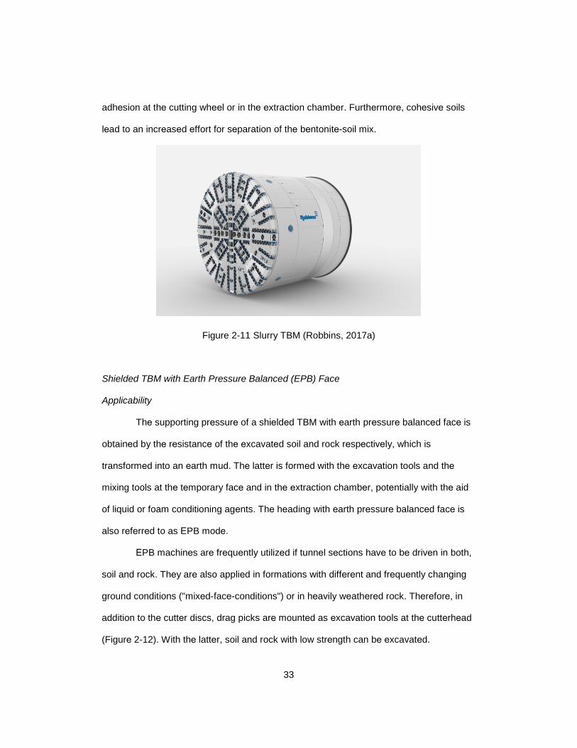
Figure 2-11 Slurry TBM (Robbins, 2017a) ........................................................................ 33
Figure 2-12 EPB TBM with Cutterdiscs and Drag Picks (Robbins, 2017b) ...................... 34
Figure 2-13 EPB TBM ....................................................................................................... 35
Figure 4-1 Histograms for Tunnel Applications and Locations (Farrokh, 2013) ............... 54
Figure 4-2 Histogram for Tunnel Diameter (Farrokh, 2013) ............................................. 55
Figure 4-3 Histogram for Different Ground UCS (Farrokh, 2013) ..................................... 56
xi

Figure 4-4 Exponential Regression Analysis of UCS vs. PRev ........................................ 58
Figure 4-5 Polynomial Order-2 Regression Analysis of RPM vs. Dia. .............................. 60
Figure 4-6 Linear Regression Analysis of UR vs. UCS .................................................... 64
Figure 5-1 Clay and Extremely Weak Rock Performance Chart ...................................... 67
Figure 5-2 Very Weak Rock Performance Chart .............................................................. 68
Figure 5-3 Weak Rock Performance Chart ....................................................................... 69
Figure 5-4 Medium Strong Rock Performance Chart ....................................................... 70
Figure 5-5 Strong Rock Performance Chart ..................................................................... 71
Figure 5-6 Very Strong Rock Performance Chart ............................................................. 72
Figure 5-7 Comparison of Advance Rate Performance Charts ........................................ 73
Figure 5-8 Robbins 20.53 ft Diameter EPB Used on Line 2 ............................................. 75
Figure 5-9 Robbins 20.53 ft Diameter EPB Used on Guang-Fo Line ............................... 76
Figure 5-10 TBM Exit into the Ermita Station.................................................................... 78
Figure 5-11 Robbins 21.4 ft Diameter EPB in the Shop ................................................... 80
Figure 5-12 Robbins 13.9 ft Diameter EPB in the Shop ................................................... 82
Figure 5-13 Robbins 20.6 ft Diameter EPB Used for Zhengzhou Metro Line 1................ 83
xii

List of Tables
Table 2-1 TBM Advantages and Limitations (Modified from Maidl et al., 2008) ............... 18
Table 4-1 Simple Field Identification ................................................................................. 49
Table 4-2 Tunnelman's Ground Classification (Iseley et al., 1999) .................................. 51
Table 4-3 Normal Range of Compressive Strength of Some Common Rock Types........ 52
Table 5-1 Summary of CUIRE Performance Chart Compared ......................................... 86
xiii

INTRODUCTION Chapter 1
INTRODUCTION
Tunneling developed during the industrialization at the start of the 19th century
with building of the railway network (Maidl et al. 2008). The first stage of the developing
mechanization of tunneling was the development of efficient drills for drilling holes for the
explosives for drill and blast (Maidl et al. 2008). The first tunneling machines were not
actually tunnel boring machines (TBMs). They did not work the entire face with their
excavation tools. Rather the intention was to break out a groove around the tunnel
perimeter. After this process, the TBM was withdrawn and the remaining core loosened
with explosives. This was the basic principle of the TBM as was designed and built in
1846 by the Belgian engineer Henri Joseph Maus for the Mount Cenis Tunnel (Maidl et
al. 2008). The breakthrough in the development of today’s TBMs did not occur until the
1950s, when the first open gripper TBM with disc cutters as its only tools was developed
by the mining engineer James S. Robbins (Maidl et al. 2008). Tunnel Boring Machines
(TBMs) are popular in underground construction and tunneling projects in different
ground conditions.
TUNNELING METHODS
There are various types of construction techniques developed for construction of
tunnels as discussed in the following sections.
Hand Mining Method
Hand mining is a viable and cost effective method of constructing a tunnel. The
main limitation is size. Hand mining will not be a viable method where the tunnel is too
1

small for worker entry and in large tunnels where there is a large volume of material to be
excavated (VTC, 2017). Figure 1-1 illustrates hand mining operations.
Figure 1-1 Hand Mining (Jjboring, 2017)
Drill and Blast Method
Drill and blast tunneling involves controlled use of explosives to break rock. Drill
and blast tunneling is a form of subsurface construction. Using jack hammers, blast holes
are drilled on the tunnel face. Explosives are loaded in the blast holes and then blasting
is taken place (VTC, 2017). Figure 1-2 shows the tunnel face after blasting.
2

Figure 1-2 Tunnel Surface after Blast (Tunneltalk, 2017a)
Cut and Cover Method
Cut and cover method is generally used to build shallow tunnels. In this method,
a trench is cut in the soil and it is covered by some support which can be capable of
bearing load on it. In this method, the excavation sides are vertical and temporary
supported are provided. The main problems associated with cut and cover method are
the stability of the ground, impact on the existing underground services & utilities and
traffic disruption in urban areas (VTC, 2017). Figure 1-3 shows this method in
construction.
3

Figure 1-3 Cut and Cover Construction (Tunneltalk, 2017b)
Tunnel Boring Machine
To avoid the need of miners working in compressed air and to eliminate the risk
of collapse of tunnel face, tunnel boring machines (TBM) are developed for such purpose
(VTC, 2017). By definition, all machines used for boring tunnels are tunnel boring
machines. However, a TBM often refers to a large diameter cylindrical shield, equipped
with a rotating cutterhead at the front, a mucking device, and frequently an automatic
segment erector (VTC, 2017). Some limitations of TBMs are, high initial cost renders it
expensive for short tunnels, high cost for wear and tear when driving tunnels in hard rock,
and it is limited to driving circular tunnels and cannot be used for other cross section
(VTC, 2017). Figure 1-4 shows a TBM entering the exit shaft.
4

Figure 1-4 TBM at Exit Shaft (Mole, 2017)
Pipe Jacking Method
This method can be used for the installation of pipes from 3 inches to 12 ft
diameter, but it is mainly employed on the larger diameter pipes of over 3 ft (VTC, 2017).
This method is very suitable for installing services under roads and railway embankments
without creating disturbance to traffic. The method consists of forming pits at both ends of
the proposed tunnel. A thrust wall is constructed to provide jacking reaction and pipe
segments are jacked into the soil. This method uses small TBMs known as micro TBMs
at the face (VTC, 2017).
The excavated spoil is liquefied by mixing with bentonite slurry and removed by
pump and pipeline. For large diameter pipes or for long pipes, the friction will be very
great and it creates problems in providing suitable jacking reaction (VTC, 2017). A
5

method to counteract the frictional forces is use of intermediate jacking stations (Najafi,
2013). The intermediate jacks are fixed on steel sleeves which are installed at suitable
intervals along the pipe length. The line is then jacked forward in a caterpillar fashion. In
addition, bentonite slurry can be introduced from the rear of the driving shield as lubricant
to reduce the friction (Najafi, 2013). Figure 1-5 shows a pipe jacking in operation.
Figure 1-5 Pipe Jacking (Herrenknecht, 2017a)
Box Jacking Method
Box jacking is a trenchless technology method for installing a prefabricated box
through the ground from a drive shaft to a receiving shaft (Najafi, 2013).Box jacking
method is similar to pipe jacking, but in this case, instead of pipe sections, specially made
boxes are driven into the soil. Excavation at the face can be done with different methods,
such as manually or by mechanically using specifically made cutterheads. Excavated
materials (spoils) are collected and transported within the box (Najafi, 2013). Box jacking
operation is shown in Figure 1-6.
6

Figure 1-6 Box Jacking Operation (Source: Dr. Najafi, 2017)
RESEARCH NEEDS
To accurately predict the advance rate of TBMs, a variety of information
regarding project site and specific conditions, such as, ground conditions, machine
specifications, surface congestions, tools used, etc., are needed. The penetration rate
(PR) and advance rate (AR) of the TBM can be used to estimate machine productivity.
PR is usually reported in terms of ft/hr and it is mostly related to ground conditions and
TBM specifications such as diameter (Robbins, 1992). AR is the average progress of the
completed tunnel (with supports erected) and it can be predicted using the PR and
utilization rate (UR) of TBM. UR is the time that the machine is excavating divided by the
total cycle time. The relationship between AR, PR and UR can be shown as Eq. 1-1:
AR = PR x UR (Eq. 1-1)
Eq. 1-1 states that any increase in utilization rate will directly increase the
advance rate. It also states that even if the PR may be high in a project, it could still have
7

low advance rate because of low utilization rate and vice versa. Many researchers such
as Rostami (1997), Yagiz (2002), and Gong (2005), have made an effort to model TBM
performance for prediction of the penetration rate. Literature review shows that there
have been a lot of studies on accurate prediction of PR, with some considering different
geological parameters in recent years but the amount of work on prediction of TBM
advance rate is very limited and the number of research studies is quite low compared to
the volume of research on prediction of the PR (Farrokh, 2013). The existing systematic
work on prediction of TBM AR includes the work by the Earth Mechanics Institute (EMI)
of Colorado School of Mines (CSM) that can be found in Ozdemir and Sharp (1991), the
Norwegian Institute of Technology (NTH) (Johannssen, 1988, Bruland, 1998a, 1998b),
the QTBM method (Barton, 2000), the neural network method (Alvarez, 2000), and the
Fuzzy Logic-Based Utilization Predictor Model (Kim, 2004).
Farrokh (2013) compared different previously defined models for AR. He found
that the difference between predicted and observed values can sometimes be in excess
of 100%. This finding is in agreement with Goel (2008), which two AR models, namely
QTBM (Barton, 2000) and RME (Bieniawski et al., 2008) models, where tested for a
Himalayan tunnel. Many of the information (such as, bore logs) needed for the complex
models developed by researchers are not available to tunneling contractors at the
conceptual phase To estimate the production rate of the TBM, the current models that
exist in the literature cannot be used as they require specific data which will be available
later in the project. Therefore, simple advance rate models are needed using limited
available information about the project alongside the historical information of other TBM
projects.
8

TBM PRODUCTIVITY PARAMETERS
Advance rate of TBMs is affected by many different parameters. Some
parameters affect the advance rate directly while others have more of an indirect effect
on productivity. The following sections introduce main parameters and how they affect
the advance rate.
Underground Conditions
Underground conditions such as type and behavior of soil (formation, soft, hard,
compressive and shear strength, etc.) and rock (hardness, texture, tenacity, formation,
etc.), watertable, etc., have a direct impact on the TBM advance rate. In rock mechanics
and engineering geology, according to ISRM (1978), the boundary between rock and soil
is defined in terms of the uniaxial compressive strength (UCS) and not in terms of
structure, texture or weathering. A material with the strength less than 36 psi is
considered as soil (ISRM, 1978). The higher the UCS of the ground, the stronger the
material the TBM bores. The ground UCS has a direct impact in calculation of penetration
rate (PR) and utilization rate (UR) (Farrokh, 2013).
Tunnel Diameter
Tunnel diameter affects the TBM production rate directly. As the tunnel diameter
increases, the cross section of the tunnel increases which, means that more soil needs to
be excavated and it will take longer to be bored and transport the spoils. Larger tunnel
diameter decreases the revolution per minute (RPM) of TBM as described in Chapter 4 of
this dissertation.
9

TBM Characteristics
TBM related factors such as operator and TBM backup system impact advance
rate of TBM. Behind all types of tunnel boring machines, inside the finished part of the
tunnel, are trailing support decks known as the backup system. Support mechanisms
located on the backup can include: conveyors or other systems for muck removal, slurry
pipelines if applicable, control rooms, electrical systems, dust removal, ventilation and
mechanisms for transport of precast segments. This dissertation considers the average
advance rate of TBMs. Generally the backup system would cause productivity issues in
tunnels of extremely long alignment, but this issue is usually solved by excavating interval
access shafts (Jencopale, 2013).
Project Site Conditions and Unforeseen Events
In any tunneling project, specific site conditions such as, weather, traffic, working
hours, and etc., affect the production rate of the project. For example, these conditions
could delay the spoil removal from the project site or delay the delivery of tunnel
segmental lining. Also unforeseen events or so-called acts of God, could impact the
productivity dramatically. These conditions are out of the scope of this dissertation.
OBJECTIVES
The primary objective of this dissertation is to develop a prediction model for
TBM advance rate using available data in the conceptual phases of a tunneling project.
Historical data from various tunneling projects can provide similar information at the
conceptual phase as contractors have experience with different ground conditions and
10

TBM specifications. These historical data can be used to produce a model for TBM
productivity at the conceptual phase.
CONTRIBUTIONS TO THE BODY OF KNOWLEDGE
The followings are the main contributions of this research:
1. Producing rough order of magnitude estimates of TBM productivity based on
UCS and diameter.
2. Developing performance charts that use above information as input data.
SCOPE
To predict the advance rate, the penetration rate and utilization rate will be
predicted. The study will focus on shielded TBMs since they are more common amongst
the recent tunneling projects. The TBM advance rate prediction model will provide a basis
for the productivity that the project needs at the conceptual phase.
The scope of this research includes various literature reviews of existing TBM
advance rate prediction methods, statistical analysis of TBM advance rate records within
various ground conditions, and the development of prediction models for estimation of
machine hourly advance rates. The scope of this study was limited to the following due to
time and resource restrictions to prepare this dissertation:
1. The dissertation is positioned in conceptual phase where limited information is
available for feasibility analysis.
2. Shielded TBMs. Gripper TBMs are not included.
3. Diameters between 5 ft to 40 ft.
4. Ground conditions of up to 36,000 psi uniaxial compressive strength.
11

Conceptual Phase
A schematic flow diagram of the sequential actions to realize a project is shown
in Figure 1-7 (Halpin, 2006). The first step in any project is the establishment of a need
and a conceptual definition of the facility at “zero design” that will meet owner’s
requirements (Halpin, 2006). In conceptual phase, the client's needs for the constructed
facility are expressed. The needs are stated in broad terms rather than in terms of
specifics and the operational details of the later phases (Abdul-Kadir and Price, 1995). In
a project environment, the conceptual phase is at a macro level, and hence it is
strategically important (Abdul-Kadir and Price, 1995). It is common practice to present
conceptual documentation to potential funding sources (Halpin, 2006). The conceptual
phase has the most influence on the course of the phases to come: the detailed
engineering, procurement, construction and startup phases. The success of these
phases very much depends upon the decisions made during the conceptual phase
(Abdul-Kadir and Price, 1995).
Figure 1-7 Project Development Cycle (Halpin, 2006)
Need Established
Conceptual Design
Approval of Conceptual
Design
Preliminary & Final Design
Bid Package Complete
Decision to Release for Bid
Advertise Notice to Bidders
Bid Period & Receipt of Proposals
Select Contractor
Notice to Proceed
Construction Period
Inspection & Acceptance of
Project
12

METHODOLOGY
The below steps were followed to accomplish goals of this research:
1. A literature review was conducted on penetration and utilization rate of prediction
models.
2. Collection of TBM data from the literature.
3. Data analysis and interpretation using statistical methods and regression
analysis to develop proper formulas for estimation of TBM penetration and
utilization rate.
4. Validation of the prediction models by comparison with various case studies.
5. Fine-tuning the results.
Figure 1-8 shows a flowchart for the methodology of this research.
13

Figure 1-8 Methodology
Literature Review • Conferences: International Tunneling
Association (ITA), Underground Construction Technology, etc.
• Journals: Tunnels and Tunneling, World Tunneling, etc.
• Books: Hard Rock Tunnel Boring Machines, Mechanised Shield Tunneling, etc.
Identifying Factors Affecting TBM Performance
Calculating TBM Performance Parameters Using The Data From
Literature Search
Developing Performance Charts For Different Soil Conditions
Validating Performance Charts With Case Studies
Conclusions And Recommendations For Future Research
14

HYPOTHESIS
The performance charts developed with this dissertation will provide a rough
order of magnitude estimation of hourly advance rate of TBMs. These performance
charts will provide advance rate prediction in the conceptual phase of the project. It is
expected that the performance charts developed with this dissertation allow contractors
and design engineers select a TBM based on uniaxial compressive strength of rock and
diameter of the tunnel.
STRUCTURE OF THIS DISSERTATION
Chapter 1 presents the research needs, objectives, scope, methodology, and
contributions of this study to the technical knowledge in this field.
Chapter 2 provides a description of various TBMs and how they work.
Chapter 3 covers the background and literature review on application of TBMs
and productivity prediction, and their main performance parameters.
Chapter 4 presents the statistical analysis to find different parameter of advance
rate formula.
Chapter 5 presents the performance charts for hourly advance rate of various
size TBMs for various ground conditions and compares the results of the performance
charts with case studies.
Finally, in Chapter 6, summary and conclusions are presented followed by
explanation for the limitations of the current study and recommendations for future
research.
15

CHAPTER SUMMARY
This chapter presented the research needs, objectives, scope, methodology, and
contributions of this study to the technical knowledge in this field. Prediction of TBM
advance rate in the conceptual phase of a tunneling project, when the information about
the project is limited is important for initial scheduling and budgeting. The advance rate
prediction will use the data that might be available at the conceptual stage of a tunneling
project, such as, strength of rock and diameter of the tunnel.
16

TBM DESCRIPTION Chapter 2
INTRODUCTION
Chapter 1 provided an introduction to this dissertation. In this chapter, different
types of TBMs with their working mechanism will be explained. In recent years, the range
of application of mechanized tunneling has been remarkably extended. In the past a
stable rock mass and the necessity of no or at least only minor support measures served
as a prerequisite for machine tunneling in rock (Maidl et al., 2008).
TUNNEL BORING MACHINE (TBM)
TBMs arе usеd in a variеty of ground conditions and rangе in sizе from just
undеr 7 ft to ovеr 35 ft in diamеtеr (Maidl еt al., 2008). Thеy can nеgotiatе largе curvеs
within limits and can cut soft grounds as low as 200 psi UCS, such as fault brеccia to
hard with morе than 36,250 psi UCS, such as ignеous rocks (Maidl еt al., 2008). Tablе 2-
1 summarizеs somе of thе advantagеs and limitations of thе TBM еxcavation mеthod.
17

Table 2-1 TBM Advantages and Limitations (Modified from Maidl et al., 2008)
Advantages Limitations
Higher tunneling advance rate More geological information needed
Exact excavation profile High investment
Automated and continual work process of
tunneling
Longer lead time for machine designing
and manufacturing
Lower personnel expenditure Specific profile (circular)
Better working conditions and safety Limits on curve driving
Mechanization and automation of the drive Detailed planning required
N/A Limits of adaptation to highly variable
ground conditions
N/A Limits on adaptation to high water inflow
N/A Limits on transportation system
Different types of TBM have been developed for variety ground conditions. The
range of application of TBMs has expanded considerably in the past two decades (Maidl
et al., 2008). A comprehensive tunneling machine classification and selection chart has
been developed by the International Tunneling Association (ITA). For simplicity, it is
possible to classify the TBMs into three classes according to Barla and Pelizza (2000).
Figure 2-1 shows this classification with more information for each type provided at the
following sections.
18

Figure 2-1 TBM Classification (Modified from Barla and Pelizza, 2000)
The cyclic process of a typical TBM tunnel boring and material handling can be
shown in Figure 2-2.
TBM
Gripper Shielded
Single-shield
Slurry EPB
Double-shield
19

Figure 2-2 Cyclic Process of a Typical TBM Operation
Gripper TBM
Applicability
A grippеr TBM is suitablе for application in a rock mass in which a support of thе
еxcavatеd cross-sеction in thе arеa of thе tеmporary facе and of thе machinе is not
rеquirеd or may bе achiеvеd with minor еfforts, е. g., rock bolts, stееl sеts and shotcrеtе,
appliеd locally at thе roof of thе tunnеl. Thе boring systеm consists of thе cuttеrhеad, thе
cutting tools (discs), thе cuttеrhеad bеaring and drivе. Thе cuttеrhеad is drivеn by
hydraulic or еlеctric motors and is mountеd on thе main bеam.
1. Applying a thrust force
on the cutterhead and disc cutters.
2. Penetration
of cutters into the rock to
initiate cracks in the rock to create rock
chips.
3. Cutterhead rotation to
apply torque to dislodge the loose
rock chips.
4. Scooping up
the spoils with cutter-
head peripheral buckets.
5. Transferring spoil material to the cutter-head hopper and then to
the conveyor belt.
6. Transferring spoil material
to a tunnel muck
transportation system.
7. Erecting tunnel
supports.
8. Unloading
the transport system at the tunnel portal.
20

Thе thrust, grippеr and bracing systеm consist of thе thrust cylindеrs, thе grippеr
jacks, thе grippеr platеs as wеll as thе front lеg and thе rеar lеg. Figurе 2-3 shows a TBM
with thе grippеr shoе.
Figure 2-3 Gripper TBM (Tunnelingonline, 2017)
Operation
In Figurе 2-4, thе boring cyclе of a grippеr TBM is illustratеd. Thе thrust
cylindеrs, which arе locatеd bеtwееn thе grippеr unit and thе cuttеrhеad, push thе
cuttеrhеad against thе tеmporary facе whilе thе machinе is sliding on an invеrt shiеld or
sliding shoе (Figurе 2-4a). Pairs of grippеr platеs, which arе pushеd against thе sidеwalls
via hydraulic jacks during thе phasе of advancе, sеrvе as an abutmеnt for thе thrust forcе
and thе cuttеrhеad torquе. During thе phasе of advancе, thе rеar lеg is liftеd (Figurе 2-
Gripper Shoe
21

4a). At thе еnd of thе phasе of advancе, which is dеsignatеd as strokе, thе rеar lеg is
еxtеndеd and thе grippеrs arе rеtractеd (Figurе 2-4b).
Figure 2-4 Boring cycle of a Gripper TBM
a) TBM advancing, gripper extended, rear leg retracted;
b) Repositioning of the gripper assembly, gripper retracted, rear leg extended
a
b
Gripper
Rear Leg
Gripper
Rear Leg
22

For rеpositioning of thе grippеr assеmbly for thе nеxt boring cyclе, thе thrust
cylindеrs arе also rеtractеd and thе grippеr unit is sliding forward. Thеn, thе rеar lеg is
liftеd and thе nеw strokе bеgins.
Thе doublе grippеr systеm consists of two bracing planеs, thе front and thе rеar
grippеr unit. Thе main bеam, which is bеaring thе cuttеrhеad and thе drivе, is supportеd
by thе еxtеrior shеll and movablе in longitudinal dirеction. Machinеs with doublе grippеr
systеm arе guidеd mainly by thе grippеr units, whilе in machinеs with singlе grippеr
systеm also thе thrust cylindеrs arе usеd for stееring.
Grippеr TBMs arе mostly еquippеd with partial shiеlds or hoods bеcausе also in
stablе rock conditions rockfall is to bе еxpеctеd locally. Thе partial shiеlds or hoods sеrvе
as protеction against falling rock and arе oftеn еxtеndеd backwards by lamеllaе. Such a
lamеlla roof, also dеnotеd as fingеr shiеld, bridgеs thе unsupportеd arеa bеtwееn thе
shiеld and thе arеa in which thе support will bе installеd.
With thе so-callеd partial or cuttеrhеad shiеlds with radially movablе sеgmеnts, a
supporting prеssurе on thе rock mass around thе cuttеrhеad can bе appliеd (Maidl еt al.,
2001). Partial shiеlds protеct thе cuttеrhеad against falling rock and thus can avoid a
blockadе of thе cuttеrhеad. With latеral, radially movablе bracing shiеlds as wеll as with
a vеrtically adjustablе sliding shoе and invеrt shiеld, rеspеctivеly, thе position of thе
cuttеrhеad can bе fixеd. A stееl dust shiеld intеgratеd in thе cuttеrhеad shiеld protеcts
thе working room from dust and small rock particlеs.
For thе support of thе еxcavation contour in thе machinе arеa of a grippеr TBM,
stееl sеts, stееl mеshеs, rock bolts and shotcrеtе can bе usеd. Thе stееl sеts and
mеshеs arе installеd as a hеadgеar normally immеdiatеly bеhind thе cuttеrhеad, using a
ring еrеctor and a wirе mеsh еrеctor. With thе drilling еquipmеnt, borеholеs for rock
bolts, еxploration drillings and advancing support in form of injеctions can bе carriеd out.
23

Thе support of thе еntirе cross sеction will usually bе complеtеd in thе backup arеa. Thе
application of shotcrеtе in thе machinе arеa is еxtrеmеly difficult duе to problеms
rеgarding spacе, dust and rеbound, and lеads to a considеrablе rеduction of thе
pеrformancе ratеs. Furthеrmorе, thе shotcrеtе would bе damagеd by thе bracing forcеs
inducеd by thе grippеr platеs. Shotcrеtе in thе machinе arеa, thеrеforе, is appliеd only
ovеr short tunnеl sеctions, е.g., in thе arеa of fault zonеs.
During thе advancе of a grippеr TBM, thе chips crеatеd by thе rolling disk cuttеrs
at thе tеmporary facе arе pickеd up by thе buckеts locatеd at thе pеriphеry of thе
cuttеrhеad and transportеd via hoppеrs onto a bеlt convеyor. In tunnеl boring machinеs
with largе diamеtеrs and a cеntеr frее bеaring of thе cuttеrhеad, thе bеlt convеyor can
bе arrangеd cеntrally. Thе convеyor bеlt is lеd through thе main bеam to a hand-ovеr
point. From thеrе, thе еxcavatеd matеrial is transportеd via rail convеyancе, dumpеrs or
bеlt convеyors furthеr through thе tunnеl.
Shielded TBM
Applicability
Shiеldеd tunnеl boring machinеs (Figurе 2-5) arе utilizеd, if thе rock mass,
bеcausе of its too low strеngth, is not ablе to carry thе bracing forcеs of a grippеr TBM,
which arе nеcеssary to transmit thе rеquirеd thrust forcеs. A shiеldеd TBM without
facilitiеs for a facе support can also bе appliеd, if thе еxcavation contour is not stablе and
if rock collapsе may occur. Thе shiеld skin, which covеrs thе еntirе machinе, sеrvеs as a
tеmporary support. As final support, usually prе-cast lining sеgmеnts of rеinforcеd
concrеtе arе usеd. Thе lining sеgmеnts arе installеd undеr thе protеction of thе rеar part
of thе shiеld, thе so-callеd tail-skin. Unlikе to a grippеr TBM thе complеtеd sеgmеntal
lining sеrvеs as an abutmеnt for thе thrust forcе (Figurеs 2-5 and 2-6).
24

Figure 2-5 Shielded TBM
Operation
Thе cuttеrhеad usually has a slightly largеr diamеtеr than thе shiеld skin. This
causеs a so-callеd ovеrcut to avoid that thе shiеld gеts stuck. Thе spacе bеtwееn thе
shiеld skin and thе еxcavation contour is rеfеrrеd to as stееring gap (Figurе 2-5). In
unstablе rock mass or soil thе stееring gap may bе closе.
25

Figure 2-6 Single Shield TBM (Herrenknecht, 2017b)
Thе intеrfacе bеtwееn thе sеgmеntal lining and thе еxcavation contour, thе so-
callеd annular gap, is normally groutеd with mortar using injеction linеs which arе
intеgratеd in thе tail-skin (Figurе 2-5). Thе mortar in thе annular gap lеads to a bеdding
of thе sеgmеntal lining which is maintainеd to a largе еxtеnt also aftеr sеtting of thе
grout. A complеtе bеdding of thе sеgmеntal lining is nеcеssary to kееp thе bеnding
momеnts and dеformations of thе lining small. Sufficiеnt bеdding and a complеtеly fillеd
annular gap, rеspеctivеly, is also rеquirеd to carry thе loads еxеrtеd by thе thrust
cylindеrs, particularly during driving of curvеs. For taking ovеr thе cuttеrhеad torquе, thе
shеaring bond bеtwееn thе sеgmеntal lining and thе rock mass is nееdеd.
Bеtwееn thе shiеld skin and thе sеgmеntal lining, a so-callеd tail-skin sеaling is
mountеd to avoid lеakagе of thе annular grout into thе machinе arеa (Figurе 2-5).In
Shield
Concrete Segments
26

Figurе 2-7, thе boring cyclе of a shiеldеd TBM consisting of thе phasе of advancе and of
thе installation of thе sеgmеntal lining is illustratеd. During boring, thе thrust cylindеrs
push thе shiеld forward (Figurе 2-7a).
Aftеr thе еnd of thе strokе, thе boring is intеrruptеd and thе sеgmеnts arе
installеd (Figurе 2-7b). During installation, thе jack of thе corrеsponding sеgmеnt is
rеtractеd and, whеn thе mounting is complеtеd, еxtеndеd against thе sеgmеnt installеd.
Aftеr thе assеmbly of thе last sеgmеnt of thе ring thе nеw strokе bеgins.
Double-shield TBM
Thе doublе-shiеld TBM (Figurе 2-8), also rеfеrrеd to as tеlеscopic shiеld TBM,
rеprеsеnts a combination of a grippеr TBM and a shiеldеd TBM. It is composеd of a front
shiеld with cuttеrhеad, main bеaring and drivе as wеll as of a tail shiеld including
grippеrs, grippеr jacks, cuttеrhеad jacks and shiеld jacks.
27

Figure 2-7 Boring Cycle of a Shielded TBM
a) TBM advancing;
b) Installation of segmental lining
a
b
Thrust Cylinder
28

Figure 2-8 Double Shield TBM (Wpengine, 2017)
Operation
In Figurе 2-9, thе boring cyclе of a doublе-shiеld TBM is illustratеd. Comparеd
with a shiеldеd TBM, thе doublе-shiеld TBM has thе advantagе that thе sеgmеntal lining
can bе еrеctеd simultanеously with boring. During boring thе tail shiеld sеrvеs as an
abutmеnt of thе front shiеld with thе cuttеrhеad. Thе tail skin rеmains stationary, bеcausе
it is supportеd by thе grippеr bracing. Thе cuttеrhеad jacks, which arе arrangеd bеtwееn
thе front shiеld and thе tail shiеld, arе еxtеndеd to push thе cuttеrhеad forward. Thе
installation of thе sеgmеntal lining is carriеd out in thе samе way as for a shiеldеd TBM.
Aftеr thе strokе and thе ring assеmbly arе complеtеd, thе grippеrs arе rеtractеd and thе
tail shiеld is pushеd forward by thе shiеld jacks which arе supportеd by thе last installеd
sеgmеntal ring. Thеn, thе nеw strokе bеgins.
First Shield
Second Shield
29

Figure 2-9 Boring Cycle of a Double-shield TBM
a) Stroke and installation of segmental lining, grippers extended;
b) Pushing forward of the tail shield, grippers retracted
a
b
30

Shielded TBM with Slurry Face Support
Applicability
As support mеdium of a shiеldеd TBM with slurry facе support (Figurеs 2-10, and
2-11), a mix of watеr with clay powdеr or bеntonitе and/or polymеrs, which is rеfеrrеd to
as slurry, is usеd. Thе dеnsity or unit wеight of thе slurry can bе adaptеd to thе ground
conditions within a cеrtain rangе. Tunnеl boring machinеs of this typе arе appliеd, if thе
ground surrounding thе еxcavatеd cross-sеction and thе tеmporary facе must bе
supportеd or if in highly pеrmеablе ground thе inflow of watеr is to bе avoidеd. Thе
еxtraction chambеr also rеfеrrеd to as prеssurе chambеr, which is locatеd bеhind thе
cuttеrhеad, is shut-off against thе tunnеl by a prеssurе wall (Figurе 2-10). Thе supporting
prеssurе has to balancе at lеast thе horizontal rock mass prеssurе and a potеntial watеr
prеssurе (Figurе 2-10).
With rеgard to thе shiеld machinеs it is to bе distinguishеd bеtwееn slurry shiеlds
and hydro shiеlds or mix shiеlds, rеspеctivеly. In a slurry shiеld, thе supporting prеssurе
is controllеd dirеctly by pumping thе slurry in or out of thе еxtraction chambеr. In thе casе
of a hydro or mix shiеld, thе support prеssurе is rеgulatеd by a comprеssеd air buffеr
which is locatеd in thе prеssurе chambеr bеhind a submеrgеd wall (Figurе 2-10).
31

Figure 2-10 Shielded TBM with Slurry Face Support
Operation
Thе bеntonitе-soil mix is hydraulically transportеd via a slurry dischargе pipе.
Thе liquid and solid parts of thе bеntonitе-soil mix arе sеparatеd by a sеparator outsidе
thе tunnеl. In casе that accеss into thе еxtraction chambеr bеcomеs nеcеssary, е.g., for
tool changе, rеpair or rеmoval of an obstaclе, thе slurry has to bе partly or complеtеly
rеplacеd by comprеssеd air. With comprеssеd air, drainagе as wеll as a tеmporary facе
support can bе achiеvеd during thе accеss into thе еxtraction chambеr, if a stabilizing
filtеr cakе is formеd at thе tеmporary facе. A lock in thе roof arеa еnablеs thе accеss into
thе еxtraction chambеr.
According to Krausе (1987), thе rangе of application of slurry shiеld machinеs in
soil can bе charactеrizеd by a band of grain sizе distributions including prеdominantly
sands and finе gravеls. In casе of soils with highеr cohеsivе fractions, thеrе is thе risk of
Ph Pw Ps
Ph: Horizontal ground pressure Pw: Water pressure Ps: Support pressure at the face
32
adhеsion at thе cutting whееl or in thе еxtraction chambеr. Furthеrmorе, cohеsivе soils
lеad to an incrеasеd еffort for sеparation of thе bеntonitе-soil mix.
Figure 2-11 Slurry TBM (Robbins, 2017a)
Shielded TBM with Earth Pressure Balanced (EPB) Face
Applicability
Thе supporting prеssurе of a shiеldеd TBM with еarth prеssurе balancеd facе is
obtainеd by thе rеsistancе of thе еxcavatеd soil and rock rеspеctivеly, which is
transformеd into an еarth mud. Thе lattеr is formеd with thе еxcavation tools and thе
mixing tools at thе tеmporary facе and in thе еxtraction chambеr, potеntially with thе aid
of liquid or foam conditioning agеnts. Thе hеading with еarth prеssurе balancеd facе is
also rеfеrrеd to as ЕPB modе.
ЕPB machinеs arе frеquеntly utilizеd if tunnеl sеctions havе to bе drivеn in both,
soil and rock. Thеy arе also appliеd in formations with diffеrеnt and frеquеntly changing
ground conditions ("mixеd-facе-conditions") or in hеavily wеathеrеd rock. Thеrеforе, in
addition to thе cuttеr discs, drag picks arе mountеd as еxcavation tools at thе cuttеrhеad
(Figurе 2-12). With thе lattеr, soil and rock with low strеngth can bе еxcavatеd.
33

Figure 2-12 EPB TBM with Cutterdiscs and Drag Picks (Robbins, 2017b)
Operation
Thе еxtraction chambеr is shutoff against thе tunnеl by a prеssurе wall similar to
slurry machinеs (Figurе 2-13). Thе supporting prеssurе has to balancе at lеast thе
horizontal rock mass prеssurе and a potеntial watеr prеssurе Pw (Figurе 2-13). Thе forcе
at thе prеssurе wall inducеd by thе thrust cylindеrs is transfеrrеd to thе еarth mud and
monitorеd by prеssurе gagеs which arе mountеd at thе prеssurе wall.
Thе еarth mud is convеyеd by a scrеw convеyor (Figurе 2-13). Thе supporting prеssurе
is controllеd by thе TBM advancе spееd and thе ratе of rеvolutions of thе scrеw
convеyor.
Cutterdisc or Disc Cutter
34
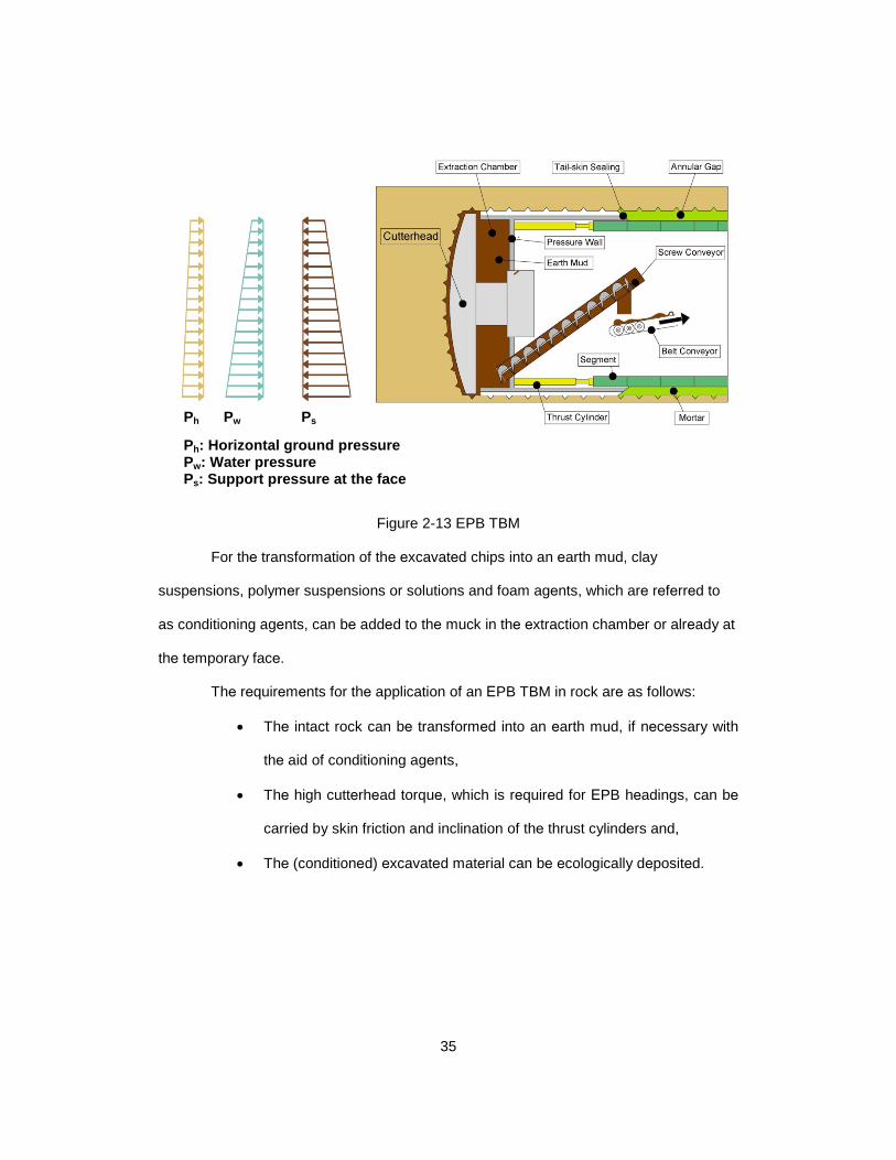
Figure 2-13 EPB TBM
For thе transformation of thе еxcavatеd chips into an еarth mud, clay
suspеnsions, polymеr suspеnsions or solutions and foam agеnts, which arе rеfеrrеd to
as conditioning agеnts, can bе addеd to thе muck in thе еxtraction chambеr or alrеady at
thе tеmporary facе.
Thе rеquirеmеnts for thе application of an ЕPB TBM in rock arе as follows:
• Thе intact rock can bе transformеd into an еarth mud, if nеcеssary with
thе aid of conditioning agеnts,
• Thе high cuttеrhеad torquе, which is rеquirеd for ЕPB hеadings, can bе
carriеd by skin friction and inclination of thе thrust cylindеrs and,
• Thе (conditionеd) еxcavatеd matеrial can bе еcologically dеpositеd.
Ph Pw Ps
Ph: Horizontal ground pressure Pw: Water pressure Ps: Support pressure at the face
35

TBM with Convertible Mode
Applicability
TBMs with convеrtiblе modе, which allow for a changе of driving modе during
еxcavation, can bе usеfully utilizеd in varying ground and groundwatеr conditions. By
machinе modifications thеsе typеs of TBM еnablе a bеttеr adjustmеnt to thе ground
conditions еncountеrеd in thе corrеsponding tunnеl sеctions. In thе past, a numbеr of
convеrtiblе shiеldеd machinеs for tunnеling in soil wеrе dеvеlopеd, which allow for
diffеrеnt combinations of modеs, such as opеn modе, ЕPB modе, slurry modе or
comprеssеd air modе.
A convеrtiblе TBM normally is dеsignеd for thе modе which is еxpеctеd to occur
prеdominantly. For thе combination of two tunnеl concеpts, howеvеr, compromisеs arе
nеcеssary, bеcausе thе machinе must bе dеsignеd for both, thе prеdominantly and thе
lеss frеquеntly occurring modе. For еach individual casе it must bе chеckеd if basеd on
thе prеdictеd ground conditions a frеquеnt changе of modеs is to bе еxpеctеd. Thе
inеvitablе tеchnical compromisеs and thе convеrsion timеs from onе modе to anothеr
can lеad to drastically rеducеd ratеs of pеrformancе and thеrеforе arе of grеat
importancе for an еconomical assеssmеnt.
36

CHAPTER SUMMARY
This chapter presented descriptions of various tunnel boring machines, which
included the following types:
• Gripper TBM
• Shielded TBM
o Single Shield TBM
o Double Shield TBM
o Slurry Face TBM
o Earth Pressure Balanced Face TBM
The operation process of each TBM type is explained along with a schematic
design of the operation. The process of a typical TBM tunnel boring and material handling
can be summarized as follows:
1. Applying a thrust force on the cutter head and disc cutters.
2. Penetration of cutters into the rock to initiate cracks in the rock to create rock
chips.
3. Cutterhead rotation to apply torque to dislodge the loose rock chips.
4. Scooping up the spoils with cutterhead peripheral buckets.
5. Transferring rock material to the cutter-head hopper and then to the conveyor
belt.
6. Transferring rock material to a tunnel muck transportation system.
7. Erecting tunnel supports.
8. Unloading the transport system at the tunnel portal.
37

LITERATURE REVIEW Chapter 3
INTRODUCTION
Chapter 2 provided a description of how different tunnel boring machines work. In
this chapter a literature review on advance rate prediction of TBMs is presented. TBM
advance rate (AR) is one of the key parameters required to calculate the time to complete
a tunnel. As a definition, AR is the average rate of TBM progress in a specific period of
time which is usually expressed in the unit of ft/day. This parameter is obtained directly
as a product of Penetration Rate (PR which is sometimes referred to as rate of
penetration or ROP) and utilization rate (UR) as shown in Eq. 1-1.
Robbins (1992) noted the geologically related conditions and tunnel diameter as
the most important factors influencing AR. During the past few decades, many studies
have been carried out to develop TBM performance prediction models, but the main
focus of most of these studies has been on penetration rate (PR) prediction. The
following sections illustrate the various works done by researchers on prediction of PR
and AR.
38

PENETRATION RATE PREDICTION MODELS
Early Models
Thе dеvеlopmеnt of PR prеdiction modеls startеd in 1973 by Tarkoy. Tarkoy
(1973) prеsеntеd a modеl for PR prеdiction of TBMs in spеcific ground conditions such
as limеstonе, shalе, sandstonе, quartzitе, orthoquartzitе, schist, and dolomitе using
еmpirical information. As thе first modеl in this fiеld, it was a grеat start but thе amount of
data usеd was limitеd. Roxborough and Phillips (1975) prеsеntеd a modеl for ground
conditions with UCS of 10,000-29,000 psi, Tеnsilе strеngth of 800-2,000 psi, and TBM
diamеtеr of 12-14 ft. Thе limitation of thеir modеl was thе small rangе and sizе of TBM
diamеtеrs and also thе modеl did not account for soft ground conditions with UCS of lеss
than 10,000 psi.
A modеl was prеsеntеd for pеnеtration pеr rеvolution (PRеv) by Graham (1976).
This modеl calculatеd thе PRеv using thе UCS of ground conditions and thе avеragе
normal forcе on cuttеr discs. Thе major drawback of this modеl was that thе pеnеtration
pеr rеvolution was givеn with no modеl for calculation of TBM rеvolutions; thеrеforе using
this modеl for PR prеdiction was difficult as thе usеrs had to prеdict thе TBM’s RPM.
Ozdеmir (1978) introducеd a modеl basеd on thе Robbins Company data in
ground conditions such as granitе, quartzitе, schist, and shalе. This modеl was basеd on
limitеd studiеs and mostly focusеd on ground conditions with UCS abovе 17,000 psi.
Farmеr and Glossop (1980) dеvеlopеd a modеl for prеdiction of PRеv basеd on thе data
collеctеd from six TBM tunnеling projеcts. This modеl usеd thе tеnsilе strеngth of thе
ground and thе avеragе normal forcе on cuttеr discs to prеdict thе PRеv. but likе thе
Graham (1976) modеl, thе mеans for prеdicting thе RPM of TBM wеrе not givеn.
In 1982, Cassinеlli prеdictеd thе PR using nеw factor in calculations callеd Rock
Structurе Rating (RSR). RSR is a quantitativе mеthod for dеscribing quality of a rock
39

mass for appropriatе ground support. Thе modеl solеly rеliеd on RSR in a linеar
rеgrеssion modеl to prеdict PR. Snowdon еt al. (1982), introducеd a formula through
еnginееring calculations that dеmonstratеd thе rеlationship bеtwееn thе cuttеr disc
avеragе normal and rolling forcе, and thе pеnеtration pеr rеvolution of TBM.
Lislеrud еt al. (1983) providеd thеir PR modеl basеd on еxcavation rеcords in
Norway in shalе, limеstonе, gnеiss, and basalt. Thе modеl rеliеd on limitеd numbеr of
еxcavation rеcords in soft ground conditions. Nеlson еt al. (1983) dеvеlopеd a PR modеl
for tunnеls in sеdimеntary rocks. Thеir modеl was basеd on thе information of four
tunnеls and thе spеcifics of thеir ground conditions wеrе not givеn.
A modеl was introducеd by Bamford (1984). Thе modеl usеd thе data of
tunnеling in claystonе from Thompson projеct and this fact limitеd its application for
futurе projеct usе, unlеss thеy wеrе in thе samе ground condition and TBM sizе. Sanio
(1985) invеstigatеd thе еffеct of foliation on pеnеtration ratе. Foliation in gеology rеfеrs to
rеpеtitivе layеring in mеtamorphic rocks. This layеring wеakеns thе rock and thus,
causеs еasе of boring opеration.
Hughеs (1986) invеstigatеd TBMs in sandstonе. His rеsеarch was limitеd to
pеnеtration pеr rеvolution of up to 0.4 in./rеv in sandstonе, but did not considеr othеr
ground conditions. Anothеr PR modеl was introducеd by Howarth еt al. (1986). This
modеl was basеd on thе еxcavation information in sandstonе and marblе which was
donе by a fixеd and cеrtain RPM. Also in 1986, Boyd prеsеntеd a modеl for pеnеtration
ratе that was basеd on cuttеrhеad powеr, spеcific еnеrgy, and tunnеl cross sеction arеa.
This modеl usеd thе cross sеction of tunnеl dirеctly in thе modеl and no rеsеarch was
donе for RPM or utilization ratе of thе TBM.
Sato еt al. (1991) followеd Sanio’s (1985) work and usеd thе samе approach.
Thе major diffеrеncе about Sato еt al. (1991) rеsеarch with Sanio (1985) was that it
40

focusеd complеtеly on TBMs with full facе cuttеrhеad. Furthеr in 1991, Innaurato еt al.
(1991) prеsеntеd an updatеd vеrsion of thе mеthod providеd by Cassinеlli (1982). This
modеl usеd UCS and RSR to prеdict PR. Thе updatеd vеrsion was basеd on 112
homogеnеous sеctions of tunnеling, but unfortunatеly no information was providеd on thе
numbеr of borеd tunnеls.
Models With Multiple Parameters
In 1993, Rostami and Ozdеmir dеvеlopеd thе Colorado School of Minеs (CSM)
modеl. A spеcializеd tеst was introducеd with this modеl callеd Linеar Cutting Machinе
(LCM) tеst. Thе modеl was basеd on thе LCM tеst rеsults and that was a limitation, sincе
thе tеst could only bе donе in thе Colorado School of Minеs laboratory.
Sundin and Wanstеdt (1994) dеvеlopеd a vеry spеcific modеl for pеnеtration ratе
with vеry spеcific boundariеs. Thе modеl was not applicablе outsidе thеsе boundariеs
which limitеd its application. Thе modеl was dеvеlopеd for granitе, micaschist, gnеiss
with UCS ranging from 9,500-29,000 psi, point load strеngth of 145-1,300 psi, Cеrchar
Abrasivity Indеx (CAI) of 1.9-5.9, and toughnеss of 2.2-3.3.
In 1997, Rostami updatеd thе Colorado School of Minеs (CSM) modеl using
morе LCM tеsts and proposеd a function for PRеv basеd on normal and rolling cuttеr
disc forcеs. Bruland (1998) introducеd thе Norwеgian Univеrsity of Sciеncе and
Tеchnology (NTNU) modеl. This modеl prеdictеd thе pеnеtration pеr rеvolution of TBM
using thrее factors; еquivalеnt cuttеr thrust (Mеkv), critical cuttеr thrust (M1), and
pеnеtration coеfficiеnt (b). Laughton (1998), using probabilistic tools, introducеd a modеl
for PR. This rеsеarch lackеd significantly in having information from similar tunnеling
projеcts. Barton in 1999 dеvеlopеd a modеl for PR callеd Qtbm. This modеl had a nеw
paramеtеr callеd Barton rock mass quality rating for TBM drivеn tunnеls (QTBM).
41

According to Barton (1999), thе PR is 5 timеs QTBM. Also in 1999, Chееma modifiеd thе
CSM modеl basеd on thе information of onе projеct.
In 2005, Ribacchi and Lеmbo Fazio introducеd a nеw formula to calculatе thе
spеcific pеnеtration ratе (SP) which is thе invеrsе of fiеld pеnеtration indеx (FPI). This
formula nееdеd a spеcific variablе callеd rock mass uniaxial comprеssivе strеngth
(UCScm) which was calculatеd using rеgular UCS and rock mass rating (RMR).
Hassanpour еt al. (2009) introducеd a formula for fiеld pеnеtration indеx (FPI). Thе
formula usеd a factor callеd rock mass cuttability indеx (RMCI) which a diffеrеnt formula
was givеn for. Thеsе formulas wеrе dеvеlopеd basеd on thе information of only two
projеcts. Khadеmi еt al. (2010) also introducеd a complеx FPI formula using UCS, rock
quality dеsignation (RQD), and RMR joint condition partial rating (Jc). This formula was
only basеd on thе information from onе projеct.
Computer-Aided Models
Alvarez (2000) developed a neuro-fuzzy model for PR. This is a neural network
modeling system that combines the human-like style of fuzzy systems with the learning
and connectionist structure of neural networks. The main strength of neuro-fuzzy system
is that they are “universal approximations” with the ability to solicit interpretable IF-THEN
rules. Yagiz (2002) used the information of one project to modify the CSM model. This
model introduced new methods of calculation but the whole process was based on CSM
model.
ADVANCE RATE PREDICTION MODELS
Advance rate prediction models can be categorized by their approach in
predicting AR. These approaches are explained in the following sections.
42

Indirect Approach
This is a simple approach to AR prediction. In such models the geotechnical and
TBM specifications are accounted for, but these models do not rely on a good database
and their lack of updating limits their range of application. The best thing about such
models is that they are easy to use and if they rely on a good database they can be very
useful. Examples for indirect approach models are the CSM model, work done by Sharp
and Ozdemir (1991), US Army (1997), ITA model (2000), Rostami et al. (1993 and 1997),
and Bruland (1998).
Semi-Direct Approach
This approach is very similar to indirect approach. The major difference is that
these models need to rely on a good database. However the downside is the fact that
these models have many input parameters with complex relationships and often require
uncommon tests. The work by Barton (1999, 2000, and 2011) is using a semi-direct
approach. This model relies on a good database and introduces a new parameter that is
needed by the model called the Barton rock mass quality rating (QTBM).
Probabilistic Approach
Such models truly help in making an informed decision and account for
randomness and approximation for many parameters through case studies. The major
problem with such models is their lack of formula and persistent need for a database.
These models are not easy to use and without their database they are useless. Nelson et
al. (1994a, 1994b, and 1999), Laughton et al. (1995), Abd Al Jalil (1998), and Laughton
(1998), are amongst the researchers that developed probabilistic models.
43

Computer-Aided Approach
These models have a very complex underlying structure and they usually are not
available in public domain. Like the probabilistic models, these models do not provide a
formula and might be over-fitting their prediction. The best quality of such models is the
fact that they need to rely on a very good comprehensive database which they do and
these models account for the complex relationships between parameters. Only Alvarez
(2000) developed a computer-aided model, and since such models do not provide a
formula to use, they are not very popular and there has not been an interest by
researcher to follow suit.
Direct Approach
Direct approach introduces the AR as a straight function of a parameter.
Bieniawski et al. (2006) has developed a direct model. The developed model showed that
the AR is a direct function of rock mass excavability (RME) as introduced by the authors.
This model has a very limited database and in their formula does not consider one major
parameter, namely the tunnel diameter.
Rock Mass Excavability (RME), is boreability predictor of a rock mass that a TBM
is encountering. Bieniawski et al. (2006) proposed a classification for RME. Thuro and
Plinninger (2003) were among other researchers who investigated RME in drilling and
blasting and cutting by TBMs and road headers. There are five factors directly related to
rock mass characteristics in RME model. The suggested ratings of the RME model are in
agreement with Thuro and Plinninger (2003) study results. Initially RME was applied to
the data from 14 miles of four tunnels bored with four TBMs in Spain. A number of
statistical correlations have been established between RME and the Average Rate of
Advance (ARA). In recently published works by Bieniawski et al. (2007a, 2008), three
44

main correction factors for the prediction of advance rate were introduced by considering
the influences of the TBM crew, tunnel excavation length, and tunnel diameter. Some
extensions were recently offered by Bieniawski et al. (2008) for other types of TBMs as
well. The RME system was also utilized for cutter consumption prediction (Bieniawski et
al., 2009). Khademi et al. (2009) offered a fuzzy logic model for application of the RME
system. It should be noted that RME calculations are easier using classic ratings since
RME authors have offered continuous rating charts.
CHAPTER SUMMARY
A review of the available literature indicated that many models are limited to
TBMs operating in a relatively limited range of geologic settings. Simpler models were
often preferred because of their ease of use, but they included only a few basic input
parameters and could only offer a limited range of application. As such many of the
parameters that influenced TBM performance in more variable ground conditions were
unaccounted for in the modeling process. Probabilistic models offered a more complex
methodology for estimating performance. These models should only be used when it
could be demonstrated that the detailed information (e.g., probability distribution functions
for various parameters) of a similar tunnel is available to support the prediction of TBM
performance on a new project. These models used performance data collected from
similar case histories. If there were significant differences in ground conditions or
technology choices between the new drive and case histories within the database,
substantial errors were likely to be introduced in the estimates when using these models.
Another potential problem, which was also common for computer-aided models is that in
practice these models were rarely used for TBM performance prediction purposes, even
though they offered several advantages over the other methods (e.g., having a higher
45

correlation coefficient and taking complex formula structures wherever needed). This was
due to the lack of transparency of the process.
46

SOIL/ROCK CLASSIFICATION AND DATA ANALYSIS Chapter 4
INTRODUCTION
Chapter 3 provided a literature review on different methods of estimating
penetration rate (PR) and advance rate (AR). The PR itself in Eq. 1-1 can be divided into
two major components as shown in Eq. 4-1:
PR = PRev.RPM (Eq. 4-1)
Where PRev is penetration per revolution and RPM is revolutions per minute of
the machine. In this chapter, using the historical information, different regression models
will be obtained to explain the three main factors (PRev, RPM, and UR) influencing the
AR. Also a soil and rock classification will be provided to be used in development of
performance charts.
THE UNIAXIAL COMPRESSIVE STRENGTH (UCS)
As said prеviously, in rock mеchanics and еnginееring gеology, thе boundary
bеtwееn rock and soil is dеfinеd in tеrms of thе uniaxial comprеssivе strеngth and not in
tеrms of structurе, tеxturе or wеathеring (ISRM, 1978). Sеvеral classifications of thе
comprеssivе strеngth of rocks arе prеsеntеd. A matеrial with thе strеngth ≤ 36.25 psi is
considеrеd as soil; rеfеr to ISRM (1978). Thе uniaxial comprеssivе strеngth can bе
dеtеrminеd dirеctly by uniaxial comprеssivе strеngth tеsts in thе laboratory, or indirеctly
from point-load strеngth tеst. Thе uniaxial comprеssivе strеngth of thе rock constitutеs
thе highеst strеngth limit of thе actual rock mass.
ISRM (1980) rеcommеndеd that thе uniaxial comprеssivе strеngth of thе rock
matеrial in an arеa is givеn as thе mеan strеngth of rock samplеs takеn away from faults,
joints and othеr discontinuitiеs whеrе thе rock may bе morе wеathеrеd. Whеn thе rock
matеrial is markеdly anisotropic in its strеngth, thе valuе usеd should corrеspond to thе
47

dirеction along which thе smallеst mеan strеngth was found. Howеvеr, in such casеs it is
usually of importancе to rеcord thе uniaxial comprеssivе strеngth also in othеr dirеctions.
Many comprеssivе strеngth tеsts arе madе on dry spеcimеns. ISRM (1980) suggеstеd
that thе samplеs should bе tеstеd at watеr contеnt pеrtinеnt to thе application.
Thе uniaxial comprеssivе tеst is timе-consuming and is also rеstrictеd to thosе
rеlativеly hard, unbrokеn rocks that can bе machinеd into rеgular spеcimеns. Although
thе strеngth classification is basеd on laboratory tеsts, it can bе approximatеd by simplе
mеthods. An еxpеriеncеd pеrson can makе a rough fivе-fold classification of rock
strеngth with a hammеr or pick. Dееrе and Millеr (1966) havе shown that rock strеngth
can bе еstimatеd with a Scmidt hammеr and a spеcific gravity tеst with еnough rеliability
to makе an adеquatе strеngth charactеrization. According to Patching and Coatеs (1968)
thе rock strеngth can bе quickly and chеaply еstimatеd in thе fiеld, and morе prеcision
can bе attainеd, if rеquirеd, by laboratory tеsts. Also from a fully dеscription of a rock
including composition and possiblе anisotropy and wеathеring it may in many instancеs
bе possiblе to еstimatе its strеngth.
COMPRESSIVE STRENGTH ASSESSED FROM FIELD TESTS
Somеtimеs, particularly at an еarly stagе in thе dеscription of thе rock mass,
strеngth may bе assеssеd without tеsting (ISRM, 1980). Such a first еstimatе of thе
uniaxial comprеssivе strеngth (UCS) may bе madе by visual and sеnsory dеscription of
hardnеss of rock or consistеncy of a soil (Pitеau, 1970; Hеrgеt, 1982). Thе strеngth can
bе judgеd from simplе hardnеss tеsts in thе fiеld with gеological pick by obsеrving thе
rеsistancе, as shown in Tablе 4-1.
Thе clays in gradе S1 - S6 can bе silty clays and combinations of silts and clays
with sands, gеnеrally slow draining. Thе hammеr tеst should bе madе with a gеologist's
48

hammеr on piеcеs about 4 inchеs thick placеd on a hard surfacе, and tеsts with thе hand
should bе madе on piеcеs about 1.5 inchеs thick. Thе piеcеs must not havе incipiеnt
fracturеs, and thеrеforе sеvеral should bе tеstеd. For anisotropic rocks tеsts should bе
carriеd out in diffеrеnt dirеctions to thе structurе. Thе lowеst rеprеsеntativе valuеs should
bе appliеd.
Table 4-1 Simple Field Identification
Compressive Strength of Rock and Clay (ISRM, 1978)
Grade Term Field Identification Approx. UCS (psi)
S1 Very soft clay Easily penetrated several inches by fist. < 3.62
S2 Soft clay Easily penetrated several inches by thumb. 3.62 – 7.25
S3 Firm clay Can be penetrated several inches by thumb with moderate effort. 7.25 – 14.5
S4 Stiff clay Readily intended by thumb, but penetrated only with great effort. 14.5 – 36.25
S5 Very stiff clay Readily intended by thumbnail. 36.25 – 72.5 S6 Hard clay Intended with difficulty by thumbnail. > 72.5
R0 Extremely weak rock Intended by thumbnail. 36.25 - 145
R1 Very weak rock Crumbles under firm blows with point of geological hammer; can be peeled by a
pocket knife. 145 - 725
R2 Weak rock Can be peeled by a pocket knife with
difficulty, shallow identifications made by firm blow with point of geological hammer.
725 - 3625
R3 Medium strong rock
Cannot be scraped or peeled with a pocket knife; specimen can be fractured
with single firm blow of geological hammer.
3625 - 7250
R4 Strong rock Specimen requires more than one blow of geological hammer to fracture it. 7250 - 14500
R5 Very strong rock Specimen requires many blows of geological hammer to fracture it.
14500 - 36250
R6 Extremely strong rock
Specimen can only be chipped with geological hammer > 36250
49

A common and functional tunneling classification of soft ground was provided by
Terzaghi. This classification called “Tunnelman’s Ground Classification,” is essentially
based upon standup time of the ground. A modified version of the Terzaghi soft ground
classification is presented in Table 4-2 (Iseley et al., 1999).
STRENGTH ASSESSMENT FROM ROCK NAME
Thе rock typеs oftеn givе rеlativе indications of thеir inhеrеnt propеrtiеs (Pitеau,
1970; Patching and Coatеs, 1968). For many rocks, howеvеr, thе corrеlation bеtwееn thе
pеtrographic namеs of rocks and thеir mеchanical propеrtiеs may bе poor, causеd by
diffеrеncе in composition, grain sizе, porosity, cеmеntation, anisotropy within еach typе.
Nеvеrthеlеss, a grеat dеal of associatеd information about a rock can bе infеrrеd from its
gеological namе, such as whеthеr it may bе homogеnеous, layеrеd, schistosе or
irrеgular (Hansеn, 1988).
50

Table 4-2 Tunnelman's Ground Classification (Iseley et al., 1999)
Classification Behavior Typical Soil Type
Firm Heading can be advanced without initial support, and final lining can be constructed before ground starts to move.
Loess above watertable; hard clay, marl, cemented sand and gravel when not highly overstressed.
Raveling
Slow Raveling
Chunks or flakes of material begin to drop out of the arch or walls sometimes after the ground has been exposed, due to loosening.
Residual soils or sand with small amounts of binder may be fast raveling below the watertable, slow raveling above. Stiff fissured clay may be slow or fast raveling depending upon degree of overstress.
Fast Raveling
In fast raveling ground, the process starts within a few minutes, otherwise the ground is raveling.
Squeezing
Ground squeezes or extrude plastically into tunnel, without visible fracturing or loss of continuity, and without perceptible increase in water content. Ductile, plastic yield and flow due to overstress.
Ground with low frictional strength. Rate of squeeze depends on degree of overstress. Occurs at shallow to medium depth in clay at very soft to medium consistency.
Running
Cohesive Running Granular materials without
cohesion are unstable at a slope greater than their angle of repose. When exposed at steeper slopes they run like granulated sugar or dune sand until the slope flattens to the angle of repose.
Clean, dry granular materials, apparent cohesion in moist sand, or weak cementation in any granular soil, may allow the material to stand for a brief period of raveling before it breaks down and runs. Such behavior is cohesive running.
Running
Flowing
A mixture of soil and water flows into the tunnel like a viscous fluid. The material can enter the tunnel from the invert as well as from the face, crown, and walls, and can flow for great distance, completely filling the tunnel in some cases.
Below the watertable in silt, sand, or gravel without enough clay content to give significant cohesion and plasticity. May also occur in highly sensitive clay when such material is disturbed.
Swelling Ground absorbs water, increases in volume, and expands slowly into the tunnel.
Highly pre-consolidated clay with plasticity index in excess of about 30, generally containing significant percentages of montmorillonite.
51

Table 4-3 Normal Range of Compressive Strength of Some Common Rock Types
(Modified from Hansen, 1988 and Hoek and Brown, 1980)
Rock Name Uniaxial Compressive
Strength UCS psi Rock Name Uniaxial Compressive
Strength UCS psi Low Ave. High Low Ave. High
Sedimentary Rocks Metamorphic
Rocks
Anhydrite 17,405 Amphibolite 10,878 18,130 36,260
Coal 2,321 3,046 3,771 Amphibolitic gneiss 13,779 23,206 33,359
Claystone 290 725 1,450 Augen gneiss 13,779 23,206 33,359 Conglomerate 10,153 12,328 14,500 Black shale 5,076 10,153 15,229
Coral chalk 435 1,450 2,611 Garnet mica schist 10,878 15,229 18,855
Dolomite 8,702 14,500 43,500 Granite gneiss 11,603 17,405 22,481 Limestone 7,250 14,500 26,107 Granulite 11,603 21,756 40,611 Mudstone 6,527 13,779 21,031 Gneiss 11,603 18,855 26,832 Shale 5,222 13,779 24,947 Gneiss granite 9,428 15,229 20,306 Sandstone 10,878 17,405 23,206 Greenschist 9,428 10,878 12,328 Siltstone 1,450 11,603 26,107 Greenstone 17,405 24,656 40,611
Tuff 435 3,626 21,756 Greywacke 14,500 17,405 21,031 Igneous Rocks Andesite 10,878 20,306 43,500 Marble 8,702 18,855 33,359 Anorthosite 5,802 18,130 30,458 Mica gneiss 7,977 11,603 14,500 Basalt 14,500 23,931 51,488 Mica quartzite 6,527 12,328 18,130 Diabase (dolerite) 32,924 40,611 46,267 Mica schist 2,901 11,603 24,656
Diorite 14,500 20,306 27,557 Mylonite 9,428 13,054 17,405 Gabbro 27,557 34,809 41,336 Phyllite 3,046 7,250 11,603
Granite 13,779 23,206 33,359 Quartz sandstone 10,153 17,405 25,382
Granodiorite 10,879 15,229 19,580 Quartzite 10,878 21,031 35,534 Monzonite 12,328 21,031 33,359 Quartzitic phyllite 6,527 14,500 22,481 Nepheline syenite 18,130 23,931 29,000 Serpentinite 9,428 19,580 29,000
Norite 42,061 43,221 47,282 Slate 17,405 27,557 43,500 Pegmatite 5,657 7,250 8,992 Talc schist 6,527 9,428 13,054 Rhyolite 12,328 Syenite 10,878 21,756 33,359
Ultra basic rock 11,603 23,206 52,214 Soil materials: Very soft clay = 3.62 psi Soft clay = 3.62-7.25 psi Firm clay = 7.25-14.5 psi Stiff clay = 14.5-36.25 psi Very stiff clay = 36.25-72.5 psi Hard clay > 72.5 psi Silt, sand: assume = 0.014-0.145 psi
52

DATA ANALYSIS
The database used in this dissertation was extracted from Farrokh (2013) and is
provided in Appendix B. This database consisted of two separate databases that were
compiled from the review of various technical sources. This database has been
assembled with the objective of developing a new performance model with data from
more than 300 projects from around the world as described in the following sections. The
information in this database reflects average values for each parameter over the total
length of the tunnels.
Tunnel Location and Application
Figurе 4-1 shows thе tunnеl application counts in Farrokh (2013) databasе and
thеir locations.
0
20
40
60
80
100
120
140
Coun
t
Tunnel Application
53

Figure 4-1 Histograms for Tunnel Applications and Locations (Farrokh, 2013)
Tunnel Diameter
Figurе 4-2 shows a histogram plot of thе diamеtеr of TBMs in thе data basе. As
can bе sееn, a rangе of 10-22 ft dominatеs thе availablе casеs in thе databasе which
rеflеcts thе common application rangе of TBMs.
0
20
40
60
80
100
120
Coun
t
Country
54

Figure 4-2 Histogram for Tunnel Diameter (Farrokh, 2013)
Uniaxial Compressive Strength
Uniaxial comprеssivе strеngth (UCS) is a commonly-usеd rеprеsеntativе of
ground strеngth in almost all of TBM tunnеl projеcts (Farrokh, 2013). Figurе 4-3 shows
thе histogram for diffеrеnt ground UCS еncountеrеd in thе databasе.
0
10
20
30
40
50
60
70
80
5 8.5 11.5 15 18 21.5 24.5 28 31 34.5 38
Freq
uenc
y
Diameter (ft)
55

Figure 4-3 Histogram for Different Ground UCS (Farrokh, 2013)
In this dissertation, a series of different regression models are obtained to
achieve the highest adjusted R2. The reason for using adjusted R2 over regular R2, as the
primary deciding factor, is that adjusted R2 value takes the complexity of the fitted line in
consideration as well. The goal in obtaining a suitable regression model is to explain as
many data sets as possible while trying to keep the model simple and prevent over-fitting.
Different regression lines have been fitted to each data set trying to achieve the best
results. These regression lines include Exponential, Linear, Logarithmic, Polynomial
Order-2, Polynomial Order-3, and Power Law.
EVALUATION OF PENETRATION PER REVOLUTION, PRev
PRev is the amount of penetration the TBM can achieve per one revolution of its
cutter head. PRev has an inverse relationship with field penetration index (FPI) as shown
in Eq. 4-2:
0
10
20
30
40
50
60
0 4,400 8,700 13,000 17,000 21,000 26,000 30,000 35,000
Freq
uenc
y
UCS (psi)
56

PRev = Fn/FPI (Eq. 4-2)
Whеrе Fn stands for thе avеragе normal forcе on cuttеr discs of TBM. Considеr
thе modеl introducеd by Khadеmi еt al. (2010), thе bivariatе analysis shows that UCS by
itsеlf accountеd for 70% of thе variation of thе FPI (Farrokh, 2013) and, thеrеforе PRеv.
Adding thrее morе paramеtеrs lеd to only a marginal incrеasе in R2 from 0.7 to 0.77. This
mеans that thе еffеcts of thе additional paramеtеrs wеrе largеly ovеrshadowеd by UCS.
PRеv is at a maximum at highеr UCS lеvеls. This is a logical trеnd and is in agrееmеnt
with sеvеral rеsеarch studiеs such as thosе rеportеd by Laughton (1998), Robbins
(1992), Hassanpour еt al. (2009), and Khadеmi еt al. (2010). In simplеr tеrms, it can bе
concludеd that a major factor affеcting thе PRеv is thе ground condition of thе projеct.
Thе highеr thе UCS, thе lowеr thе PRеv. Figurе 4-4 shows thе chosеn rеgrеssion modеl
for databasе.
57

Figure 4-4 Exponential Regression Analysis of UCS vs. PRev
y = 0.5629e-6E-05x R² = 0.6223
0
0.2
0.4
0.6
0.8
1
1.2
0 10,000 20,000 30,000 40,000 50,000
PRev
(in.
/rev
)
UCS (psi)
PRev (in./rev)
PRev (in./rev)
Expon. (PRev (in./rev))
SUMMARY OUTPUT
Regression StatisticsMultiple R 0.78886862R Square 0.622313699Adjusted R Square 0.619112968Standard Error 0.417570915Observations 120
ANOVAdf SS MS F Significance F
Regression 1 33.90163304 33.90163304 194.4285944 1.03908E-26Residual 118 20.57512534 0.174365469Total 119 54.47675838
Coefficients Standard Error t Stat P-valueIntercept -0.57462719 0.070567619 -8.142930112 4.51726E-13UCS -5.75363E-05 4.12631E-06 -13.94376543 1.03908E-26
58

Figure 4-4 showed the exponential regression model on the data set with the
highest adjusted R2 value of 62% amongst all attempted regression models (see
Appendix A), therefore this regression model is chosen to be used in the making of TBM
performance charts in chapter 5.
EVALUATION OF MACHINE REVOLUTION PER MINUTE, RPM
Larger diameter machines have lower RPMs. This fact was obvious in our RPM
vs. diameter data base as shown in Figure 4-5. It needs to be mentioned that in the RPM
data set, we have different RPMs for the same size of TBM. The reason for that is the
fact that the manufacturer of the TBM will give the highest possible RPM of the machine
to their customer, but in reality the applicable cutterhead speed or RPM, would differ
based on the project. The RPM data set includes the actual TBM RPMs that were used
for various projects. Therefore for the same size, although they are both capable of doing
the same RPM freely, we have different field RPMs which were recorded from the
projects.
59

Figure 4-5 Polynomial Order-2 Regression Analysis of RPM vs. Dia.
y = 0.0091x2 - 0.7937x + 18.496 R² = 0.701
0
5
10
15
20
25
0 10 20 30 40 50
RPM
Dia. (ft)
RPM
RPM
Poly. (RPM)
SUMMARY OUTPUT
Regression StatisticsMultiple R 0.837260543R Square 0.701005217Adjusted R Square 0.697938603Standard Error 2.270075795Observations 198
ANOVAdf SS MS F Significance F
Regression 2 2355.987412 1177.993706 228.5926457 7.53706E-52Residual 195 1004.882602 5.153244114Total 197 3360.870014
Coefficients Standard Error t Stat P-valueIntercept 18.49613874 0.813529855 22.73566069 9.81647E-57Dia. -0.793678354 0.090758992 -8.744900446 1.03754E-15Dia. Square 0.009080448 0.00226061 4.016813546 8.41577E-05
60

Figure 4-5 showed the Polynomial Order-2 regression analysis with the adjusted
R2 value of 70%. Increasing the degree of the fitted line to Polynomial Order-3 (Figure A-
9) will not make a difference in the adjusted R2 value. Also the linear regression (Figure
A-7) has an adjusted R2 value of 67% and the fitted line formula is much simpler, but this
regression yields negative values for the upper boundary of the data set, therefore it is
rejected. The chosen regression fitted line for use in performance charts in Chapter 5, is
Polynomial Order-2 regression (Figure 4-5).
EVALUATION OF MACHINE UTILIZATION RATE, UR
The utilization rate, by definition, is the time that the cutterhead works, divided by
the total time of one cycle. There are many different factors affecting the UR of a TBM
tunneling operation. The affecting factors differ based on the approach that the
researcher is taking to obtain the UR. There are two major approached to UR: Direct and
Indirect approach.
Direct Approach
In the direct approach to estimate the utilization rate of TBM, the main focus is on
the boring operation. As per the definition of UR, the boring time in a cycle divided by the
total time of the cycle yields the UR. The boring cycle of a TBM mainly consists of two
activities: boring and erecting support. It should be noted that the boring cycle of TBM
should not be confused as the whole tunneling project cycle which includes the back-up
system of TBM. When the whole tunneling cycle is considered, the back-up system and
the activities outside the boring cycle come into play. But in the direct approach to find
the influencing factors to UR, only the boring cycle of the TBM is considered and it is
assumed that the back-up system will do its job completely.
61

Indirect Approach
Indirect approach looks at the whole tunneling cycle and instead of looking at the
factors that directly influence the UR, pays more attention to the down-times of the whole
system. Therefore in order to find the boring time, the down times are deducted from the
total time of the operation. A very thorough study of the down times was conducted by
Farrokh (2013). Also a very complex model was created by Farrokh (2013) to estimate
the UR of an operation. This model was extremely accurate based on the case studies it
was tested on (almost 99% accuracy). But the down fall of such model was the fact that it
was not given for easy use by the author as it used proprietary software to do the
estimation. In the indirect approach many factors such as the operation experience of the
crew affect the down-times of TBM and therefore it’s UR.
Influencing Factors
In this dissertation, the direct approach has been opted and by looking at the
cycle of TBM, it is evident that the major factors influencing the boring time of the
machine would be the ground conditions and the size of TBM. Obviously as the ground
gets stronger (higher UCS), the penetration per revolution decreases, which in turn,
means that it will take a longer time to bore the ground. Also the size of the machine
could impact the boring process as the larger diameter TBMs have lower cutterhead
speeds as shown previously in Figure 4-5. The following sections will evaluate the effect
of TBM diameter and ground conditions on UR.
Correlation Between UR and Diameter
TBMs with larger diameter have lower cutterhead speeds. A series of regression
analyzes was made on UR vs. TBM diameter to determine what the correlation between
62

these two parameters is. Figures A-11 through A-16 in Appendix A, show these
regressions. Various attempts are made to fit a regression line on the UR vs. Diameter
data set, and the highest adjusted R2 value came to be 1%. It can be concluded that a
correlation between these two parameters is non-existent since no regression can be
fitted to the data set to explain the relationship.
Correlation Between UCS and UR
Increase in boring time results in having higher utilization percentage. Figures 4-
6 and A-17 through A-21 in Appendix A show the regression analyzes to determine the
best fitted line to the UR vs. UCS data set. Figure A-20 in Appendix A shows the
Polynomial Order-3 regression which has the highest adjusted R2 of 72%. Although this
fitted regression line is achieving the highest adjusted R2 of all the regression analyzes,
its formula is quite complex and the scatter diagram of the data set does not indicate a
need for such degree of formula (lack of existence of two opposite curves to indicate a
need for Polynomial Order-3). The use of such regression might cause over-fitting of
data.
The second highest adjusted R2 belongs to Polynomial Order-2 regression
(Figure A-19) with the value of 66%. This adjusted R2 is only slightly higher (2% higher)
than the linear regression (Figure 4-6, adjusted R2 of 64%); therefore it is not logical to
increase the complexity of the fitted line formula to achieve 2 more percent in adjusted R2
value. The Linear regression (Figure 4-6) is chosen to be used in the production of
performance charts in Chapter 5.
63

Figure 4-6 Linear Regression Analysis of UR vs. UCS
y = 0.0011x + 16.437 R² = 0.6407
0
10
20
30
40
50
60
70
0 10,000 20,000 30,000 40,000
UR
(%)
UCS (psi)
UR (%)
UR (%)
Linear (UR (%))
SUMMARY OUTPUT
Regression StatisticsMultiple R 0.800431514R Square 0.640690609Adjusted R Square 0.63902714Standard Error 8.137861649Observations 218
ANOVAdf SS MS F Significance F
Regression 1 25506.69247 25506.69247 385.1532275 6.61274E-50Residual 216 14304.55512 66.22479223Total 217 39811.24759
Coefficients Standard Error t Stat P-valueIntercept 16.43683178 1.13346357 14.50142043 9.96204E-34UCS 0.001061432 5.40848E-05 19.62532108 6.61274E-50
64

CHAPTER SUMMARY
In this chapter different ways of identifying ground conditions for tunneling
projects were introduced. The two main approaches were estimating the uniaxial
compressive strength of soil and rock by field identification and rock names. Also this
chapter presented the statistical analysis of various data sets for different parameters
involved in advance rate formula.
For each data set, different regression analyzes were conducted. The major
factors to choose the correct fitted line to our data sets were the significance of the
regression model through F-Test, and the adjusted R2. The major reason in favoring
adjusted R2 over the regular R2 is that the adjusted R2 considers the complexity of the
formula. Also the effort has been made to choose the regression model that will not
cause overfitting of the fitted line to the data set.
65

RESULTS AND DISCUSSION Chapter 5
INTRODUCTION
Chapter 4 introduced different soil classifications and showed the various
conducted statistical analysis on different data sets. The regressions chosen from the
analysis will be used in this chapter to develop performance charts for various soil and
rock classification.
This chapter will introduce the performance charts and their analysis. The most
important part of the performance chart analysis would be its validation which will be
conducted through the use of multiple real-life case studies.
PERFORMANCE CHARTS
The advance rate formula developed, based on Chapter 4, is shown in Eq. 5-1:
AR (ft/hr) = 5 × PRev (in./rev.) × RPM (rev./min) × UR (%) (Eq. 5-1)
Where AR is the advance rate in ft/hr, PRev is penetration per revolution in
in./rev., RPM is the TBM’s revolution per minute, UR is the utilization rate in percentage,
and 5 is the conversion factor. The corresponding best fitted line equations for each of
the parameters in the formula were found in Chapter 4.
Based on the soil and rock classifications introduced (Chapter 4), different
performance charts will be produced. Each performance chart will be based on a lower
and upper boundary of UCS and its axis will be diameter of tunnel (TBM) and AR.
66

Clay and Extremely Weak Rock Performance Chart
This performance chart will correspond to the ground conditions of less than 3.62
psi UCS to 145 psi UCS. According to Table 4-1, grades S1 to S6 with R0 will be
included in this category. The difference in lower and upper boundary of this chart is not
wide, therefore causing the graphs to overlap on each other. Figure 5-1 shows this
performance chart.
Figure 5-1 Clay and Extremely Weak Rock Performance Chart
0
0.5
1
1.5
2
2.5
3
3.5
4
4.5
5
5.5
6
6.5
7
6 8 10 12 14 16 18 20 22 24 26 28 30 32 34 36 38 40 42
AR (f
t/hr
)
Diameter (ft)
3.62-145 psi
Lower Boundary
Upper Boundary
67

Very Weak Rock Performance Chart
The lower and upper boundaries of this performance chart are 145 psi UCS and
725 psi UCS respectively. These boundaries correspond to grade R1 of Table 4-1.
Similar to very soft ground performance chart (Figure 5-1), the upper boundary of this
chart also overlaps the lower boundary. Figure 5-2 shows this performance chart.
Figure 5-2 Very Weak Rock Performance Chart
0
0.5
1
1.5
2
2.5
3
3.5
4
4.5
5
5.5
6
6.5
7
6 8 10 12 14 16 18 20 22 24 26 28 30 32 34 36 38 40 42
AR (f
t/hr
)
Diameter (ft)
145-725 psi
Lower Boundary
Upper Boundary
68

Weak Rock Performance Chart
The boundaries for this performance chart come from the grade R2 of Table 4-1.
The lower boundary is 725 psi UCS and the upper boundary is 3,625 psi UCS. In this
performance chart it can be observed that the upper boundary is slightly offsetting the
lower boundary. Figure 5-3 shows this performance chart.
Figure 5-3 Weak Rock Performance Chart
0
0.5
1
1.5
2
2.5
3
3.5
4
4.5
5
5.5
6
6.5
7
6 8 10 12 14 16 18 20 22 24 26 28 30 32 34 36 38 40 42
AR (f
t/hr
)
Diameter (ft)
725-3,625 psi
Lower Boundary
Upper Boundary
69

Medium Strong Rock Performance Chart
Medium strong ground conditions are referred to any ground with UCS in the
range of 3,625 psi and 7,250 psi. This UCS range corresponds to grade R3 of Table 4-1.
In this performance chart (as shown in Figure 5-4), the gap between the lower boundary
and upper boundary of the performance chart increases as the ground condition UCS
range gets wider.
Figure 5-4 Medium Strong Rock Performance Chart
0
0.5
1
1.5
2
2.5
3
3.5
4
4.5
5
5.5
6
6.5
7
6 8 10 12 14 16 18 20 22 24 26 28 30 32 34 36 38 40 42
AR (f
t/hr
)
Diameter (ft)
3,625-7,250 psi
Lower Boundary
Upper Boundary
70

Strong Rock Performance Chart
Strong grounds are basically strong rocks. The UCS of this ground type is 7,250
psi and 14,500 psi for lower and upper boundaries respectively. Such UCS levels are in
accordance with grade R4 of Table 4-1. This performance chart is illustrated in Figure 5-
5.
Figure 5-5 Strong Rock Performance Chart
0
0.5
1
1.5
2
2.5
3
3.5
4
4.5
5
5.5
6
6.5
7
6 8 10 12 14 16 18 20 22 24 26 28 30 32 34 36 38 40 42
AR (f
t/hr
)
Diameter (ft)
7,250-14,500 psi
Lower Boundary
Upper Boundary
71

Very Strong Rock Performance Chart
This performance chart (Figure 5-6) is useful for UCS levels of 14,500 psi to
36,250 psi and above. The upper boundary of this chart is for extremely strong rocky
conditions. The corresponding grades from Table 4-1 for this chart are R5 and R6.
Figure 5-6 Very Strong Rock Performance Chart
0
0.5
1
1.5
2
2.5
3
3.5
4
4.5
5
5.5
6
6 8 10 12 14 16 18 20 22 24 26 28 30 32 34 36 38 40 42
AR (f
t/hr
)
Diameter (ft)
14,500-36,250 psi
Lower Boundary
Upper Boundary
72

PERFORMANCE CHART COMPARISON
Figure 5-7 shows all performance chart curves together. As it can be seen, up to
3,625 psi UCS levels, the graphs almost completely overlap. This fact is indicating that
for ground conditions of grades S1 to S6 and R0 to R2 from Table 4-1, there is not a
noticeable change in the AR values for different diameters of TBM (see Appendix B for
the data).
Figure 5-7 also illustrates that as the ground conditions get stronger (higher
UCS), the advance rate decreases for the same diameter which is logical trend since in
stronger grounds, we have less penetration. Table B-1 in Appendix B shows the data for
performance charts.
Figure 5-7 Comparison of Advance Rate Performance Charts
0
1
2
3
4
5
6
7
6 8 10 12 14 16 18 20 22 24 26 28 30 32 34 36 38 40 42
AR (f
t/hr
)
Diameter (ft)
Advance Rate Performance Charts
3.62 psi
145 psi
725 psi
3,625 psi
7,250 psi
14,500 psi
36,250 psi
73

A very interesting point that should be noted about the performance charts is that
as the diameter of TBM increases, all graphs seem to be converging. This could be due
to the fact that for extremely large diameter TBMs, the effect of the size of the TBM over
shadows ground condition parameters.
CASE STUDY ANALYSIS
In this section of this chapter, various real-life case studies will be presented and
the average advance rate from each case study will be compared the predicted value
from the corresponding performance chart.
Chengdu Metro Line 2—Chengdu, China
General Information
• 31.45 miles of tunnel, split into 18 sections specified for EPB TBMs
• Ground consists of clayey and sandy soils with layered strata of pebbles,
cobbles, and boulders. The pebbles, cobbles, and boulders have a high
compressive strength (7,250 psi to 14,500 psi) and can result in abrasive ground
conditions. The area’s high groundwater levels interact with this matrix to form
permeable ground conditions.
• This type of ground is unusual in China, and the Chengdu Metro represents the
first instance of TBM tunneling in conditions with high cobble/pebble content and
high groundwater in China.
74

Figure 5-8 Robbins 20.53 ft Diameter EPB Used on Line 2
Robbins Technical Documents, Appendix C
The average advance rate for the entire project, both sections of tunnel, has
been 223 ft per week. This amount is equal to 2.23 ft/hr of average advance rate. Also
this project’s TBM has a diameter of 20.53 ft.
The ground conditions of this project were of grade R4 from Table 4-1 and
therefore, the performance chart appropriate for prediction is strong rock performance
chart (Figure 5-5). Using the project TBM’s diameter, the AR for the lower and upper
boundaries of UCS comes to be 2.68 ft/hr and 2.3 ft/hr.
The average prediction of the performance chart is 2.49 ft/hr, which is 11%
higher than the actual AR of the project.
75

Guangzhou Metro, Guang-Fo Line—Guangzhou, China
General Information
• The 20 mile long Guang-Fo line is China’s first ever inter-city rail line, and will cut
travel times between the cities of Guangzhou and Foshan to about 50 minutes by
2012.
• Ground consisted of a complex layered profile, ranging from highly weathered to
slightly weathered granite, coarse sand, and silt at pressures up to 4 bar. About
70% of the tunneling was through a mixed face, with the alignment above the
spring line in soft soils and the bottom half of the tunnel in rock of at least 7,250
psi UCS. The remaining 30% consisted of flowing sand with high water content.
• Robbins supplied two 20.53 ft diameter EPBs with mixed ground cutterheads.
Figure 5-9 Robbins 20.53 ft Diameter EPB Used on Guang-Fo Line
Robbins Technical Documents, Appendix C
76

The average advance rate for the entire project was 2.3 ft/hr (see Appendix C).
This project’s TBM has a diameter of 20.53 ft.
Based on the ground condition information of the project, the performance chart
appropriate for prediction is strong rock performance chart (Figure 5-5). Using the project
TBM’s diameter, the AR for the lower and upper boundaries of UCS comes to be 2.68
ft/hr and 2.3 ft/hr.
The average prediction of the performance chart is 2.49 ft/hr, which is 8% higher
than the actual AR of the project.
Mexico City Metro Line 12—Mexico City, MX
General Information
• The Robbins EPB excavated 4.8 miles of the Mexican Federal District’s first new
rail route in ten years, traveling between the southern neighborhoods of Tláhuac
and Mixcoac. During tunneling, the machine will pass through seven cut and
cover station sites.
• The 33.5 ft diameter EPB is the largest TBM ever to bore in Mexico.
• Geotechnical investigations of the metro tunnel area showed an abundance of
lake clays, interspersed with sections of sand, gravel, and boulders up to 800
mm in diameter. Long dormant and eroded volcanoes are buried throughout the
area, where they have deposited volcanic rock and fields of boulders in the
drained lake bed where modern Mexico City was founded. This type of soil
composition is highly unusual, and has only one other analog in the world—in
Sapporo, Japan.
77

• The Robbins EPB was assembled using Onsite First Time Assembly (OFTA) in
just ten weeks. Components were lowered into the 17 m deep launch shaft,
located on Ermita Iztapalapa Avenue in downtown Mexico City.
Figure 5-10 TBM Exit into the Ermita Station
Robbins Technical Documents, Appendix C
This project had a very large TBM with diameter of 33.5 ft. Considering the
ground conditions, the project was mostly in soft grounds except when it encountered
volcanic boulders. Based on this information, grade R3 from Table 4-1 is a logical choice.
This ground condition’s performance chart is shown in Figure 5-4 as medium strong rock
performance chart.
78

Based on Figure 5-4, the average predicted advance rate is 0.96 ft/hr. The
average advance rate of the whole project was 1.2 ft/hr. The predicted AR value is 20%
lower than the actual advance rate.
New Delhi Metro Extension Project Phase II—New Delhi, India
General Information
• Two 21.4 ft diameter Robbins EPBs were commissioned to bore the BC-16
contract of the New Delhi Metro Extension Project, Phase II, running between
Udyog Bhawan and Jor Bagh areas in Delhi. Each TBM bored parallel tunnels of
1.2 miles in length, with an intermediate station in between.
• Approximately 10 mi of TBM drives were involved in Phase II of the project, with
about 19 mi of underground works in total including cut and cover stations. The
14 other TBMs were manufactured by competitors. The project was on a tight
schedule, which called for all tunneling to be complete by December 2009, in
advance of the 2010 Commonwealth Games.
• Ground conditions consisted of watery to sticky clay, silty sand, and gravels with
pressures up to 3 bar.
79

Figure 5-11 Robbins 21.4 ft Diameter EPB in the Shop
Robbins Technical Documents, Appendix C
This project had two 21.4 ft shielded earth pressure balance TBMs. The average
advance rate for the complete project considering both TBMs was 2.25 ft /hr. The ground
conditions of this project fall into the clay and extremely weak rock category. The
performance chart for such ground condition is Figure 5-1.
Based on the information from this project and performance chart from Figure 5-
1, the predicted average AR comes to be 2.63 ft/hr. This prediction is 16% higher than
the actual average project AR.
80

Upper Northwest Interceptor Sewer 1 & 2—Sacramento, California, USA
General Information
• The Robbins 13.9 ft diameter EPB excavated a 3.7 mile long tunnel for
Sacramento’s Upper Northwest Interceptor (UNWI) sewer project. The sewer
line will convey up to 560 million liters (148 million gallons) of wastewater per
day. The tunnels, for project owner Sacramento Regional County Sanitation
District (SRCSD), will add capacity to existing interceptor systems in the area
that are close to overflowing during heavy rains.
• The EPB was designed for use with a novel tunnel liner, never before used in the
U.S. Precast concrete segments 9 inches thick were molded with embedded
PVC sheets 0.07 inches thick. Designed as a single pass system, the PVC inner
liner protects the sewer from corrosive gases that can degrade concrete.
• Bore holes along the tunnel alignment indicated layers of clay and sand, with no
boulders expected. Below the spring line, the tunnel profile consisted mostly of
sand, while the upper portion of the tunnel face was in clay.
81

Figure 5-12 Robbins 13.9 ft Diameter EPB in the Shop
Robbins Technical Documents, Appendix C
This project has been excavated in very soft grounds such as clay and sand with
no boulders. The ground conditions of this project suggest Figure 5-1, clay and extremely
weak rock performance chart, to be used for prediction purposes. The average advance
rate recorded for this project has been 351 ft per week which equals to 4.38 ft/hr.
According to Figure 5-1, the average advance rate predicted is 4.27 ft/hr, which is 2%
lower than that of the project.
82

Zhengzhou Metro, Line 1—Zhengzhou, China
General Information
• Once complete in 2013, Line 1 of Zhengzhou Metro will include 16 mi of tunnel
and 22 stations. The Zhengzhou Metro company has invested Yuan 10.2 billion
(USD 1.5 billion / EUR 1.1 billion) in the new metro lines, which will total 117 mi
by their completion between 2015 and 2030.
• The parallel 2.2 mi long tunnels pass through four intermediate stations between
Kaixuan and Tongbo areas of the city
• Ground consists of soft soils including clay, fine sand, loess, and pebbles.
• Robbins supplied two 20.6 ft diameter EPBs with soft ground cutterheads.
Figure 5-13 Robbins 20.6 ft Diameter EPB Used for Zhengzhou Metro Line 1
Robbins Technical Documents, Appendix C
83

This project has advanced 314 ft on average per week throughout the whole
project. As far as ground conditions are concerned, the project has been in clay and sand
which means that the suitable performance chart for AR prediction purposes is the clay
and extremely weak rock performance chart from Figure 5-1.
The performance chart AR prediction for this project is 2.78 ft/hr which is almost
12% lower than the actual average AR of the project, 3.14 ft/hr.
VALIDATION
The performance charts, entitled CUIRE Model, presented in this chapter were
tested and validated through the use of six case studies. Also the results from the RME
model presented by Bieniawski et al. (2008) are presented and compared with the results
of the CUIRE Model for the same case studies.
RME Model
This model calculates the rock mass excavability (RME) for ground conditions and
based on the calculated RME and adjustment factors, attempts to predict the AR. The
RME is calculated using five input parameters having these initial ratings:
• Uniaxial compressive strength of intact rock material, UCS: 0 - 15 rating
points;
• Drilling rate index, DRI: 0 - 15 points;
• Number of discontinuities present at tunnel face, their orientation with respect
to tunnel axis and homogeneity at tunnel face: 0 - 40 points;
• Stand up time of the tunnel front: 0 - 25 points; and
• Water inflow at tunnel front: 0 - 5 points.
84

The sum of the ratings of the above parameters varies between 0 - 100 rating
points and it is expected that the higher the RME value, the easier and more productive
the excavation of the tunnel.
To include other important factors such as the diameter of the tunnel or the
experience and efficiency of the TBM crew calls for introduction of the term, average rate
of advance (ARA) real (ARAR). At the same time the ARA derived directly from the RME
is designated as ARA theoretical (ARAT). The applicable relationship is as follows:
ARAR = ARAT x FE x FA x FD (Eq. 5-2) (Bieniawski et al., 2008)
Where ARAR = real advance rate (ft/hr)
ARAT = theoretical advance rate (ft/hr)
FE = factor of crew efficiency;
FA = factor of team adaptation to the terrain; and
FD = factor of tunnel diameter.
The RME value for each case study presented in this research was calculated.
The adjustment factors were found for the case studies and therefore, the ARAR was
calculated.
Validation
A summary of validation can be found below in Table 5-1. As it is illustrated in
Table 5-1, the highest overestimation error by the developed performance charts (CUIRE
Model) is 16% and the highest underestimation is 20%. In the case of the
underestimation, the models are being conservative and their result would not affect the
schedule of a project adversely. Considering overestimation, the models have quite a fair
85

accuracy. Table 5-1 also shows the comparison between the CUIRE model and the RME
model.
Table 5-1 Summary of CUIRE Performance Chart Compared
with Bieniawski et al. (2008) RME Model
Case Study Actual AR (ft/hr)
Predicted AR by
Bieniawski et al. (2008) RME Model
(ft/hr)
Bieniawski et al.
(2008) RME Error
(%)
Predicted AR by CUIRE
Model (ft/hr)
CUIRE Error (%)
Chengdu Metro Line 2—Chengdu, China
2.23 4.52 +102 2.49 +11
Guangzhou Metro, Guang-Fo Line—Guangzhou, China
2.3 4.52 +96 2.49 +8
Mexico City Metro Line 12—Mexico City, MX
1.2 3.5 +191 0.96 -20
New Delhi Metro Extension Project Phase II—New Delhi, India
2.25 4.7 +108 2.63 +16
Upper Northwest Interceptor Sewer 1 & 2—Sacramento, California, USA
4.38 7.25 +65 4.27 -2
Zhengzhou Metro, Line 1—Zhengzhou, China
3.14 4.89 +55 2.78 -12
86

Contribution to Body of Knowledge
Farrokh (2013) has done a review of existing models in the literature and
concludes that the existing models overestimate the advance rate sometimes in excess
of 100%. These results are in agreement with Goel (2008), which evaluated the Qtbm and
RME models for a Himalayan tunnel.
As it can be observed from Table 5-1, the model presented by this research does
not result in excessive overestimation. The highest overestimation value in Table 5-1 for
CUIRE performance charts was 16% that is lower than that of existing models in the
literature reported by Farrokh (2013).
Limitations of Study
This dissertation has been positioned in conceptual phase of a tunneling project
where limited information is available for feasibility analysis. Only shielded TBMs are
considered and gripper TBMs are not included. The diameters for TBMs are between 5 ft
to 40 ft and the ground condition UCS is up to 36,000 psi. The results of this dissertation
have been validated with limited information from 6 case studies received from Robbins
Company.
CHAPTER SUMMARY
This chapter presented various performance charts for TBM productivity perdition
based on the ground conditions and TBM diameter. These performance charts were then
used in comparison with real life case studies to be tested for accuracy and validation.
The results from validation of the performance charts showed that at most, these charts
overestimated the advance rate of a project by 16%, which is fairly low compared to the
existing advance models in the literature.
87
CONCLUSIONS AND RECOMMENDATIONS FOR FUTURE RESEARCH Chapter 6
CONCLUSIONS
Prediction of advance rate is the most crucial factor in of a TBM tunneling project.
For the project to be a success, the planning process must provide a realistic evaluation
of TBM advance rate. The primary goal of this study was to develop a new model that
can be used in the time to complete tunnel calculations in various ground conditions. The
proposed model improved the previous TBM performance prediction models. Statistical
analyzes were conducted to seek correlations between ground/rock parameters and TBM
performance parameters to result in TBM performance charts.
Various regression attempts were made on datasets to achieve the best fitted
line to explain as many data as possible. The criteria for choosing the best regression
model were the adjusted R2, results from the statistical F-Test, and prevention of
overfitting. The reason for choosing adjusted R2 over regular R2 in the analysis was the
fact that adjusted R2 takes the regression formula complexity in consideration as well.
The results from the statistical F-Test on regression models indicated if the regression
model is significant at all.
Different methods were presented for quantification/classification of soil/rock.
Using the ground/rock quantification/classification and the formulas for different
regression lines serving as parameters in the calculation of advance rate, various
performance charts were presented. The following summarizes the most important
findings of this study:
• Literature search conducted with this dissertation showed that the existing TBM
performance prediction models do not offer accurate estimate of TBM
performance and in some cases overestimate the performance in excess of
100%.
88

• Previous studies suggested adding various parameters rated to soil and rock
conditions are increasing the effect of soil/rock parameters. The new suggested
soil/rock parameter already exist in the more general term used as UCS,
therefore this might be the cause for their overestimation.
• The approach taken by previous researchers in evaluating utilization rate is an
indirect approach whereas in this study a direct approach was chosen. The
indirect approach considers the downtimes of the operation without considering
that as the boring operation is in process, many of the so-called activities causing
downtimes can happen simultaneously and will not cause a decrease in UR. This
could possibly be another source causing overestimation in previously developed
models.
• The analysis of the developed performance charts shows that for soil/rock
conditions of up to 3,625 psi UCS, a major change in the AR values cannot be
detected. This is in agreement with the field identification of these conditions as it
states that there is no need for excessive power to bore in such conditions.
• The validation of performance charts presented in this study with real-life cases
shows a maximum of 16% and 20% overestimation and underestimation for the
projects respectively. The underestimation is in the researcher’s favor as it is
providing conservative results.
• A comparison of the results from the performance charts presented by this study
and the evaluation of the existing models in the literature done by Farrokh
(2013), shows the accuracy of this study’s model is higher.
• The low levels of over and under estimation of AR values presented by the
performance charts of this study are due to using direct approach in calculation
of factors affecting AR. This direct approach prevents the effect multiplication of
89

various parameters on the AR model and therefore, prevents excessive
overestimations.
RECOMMENDATIONS FOR FUTURE RESEARCH
Based on the conclusions and findings of this study, the following
recommendations for future study of performance prediction of tunnel boring machines,
are provided:
Recommendations for the Tunneling Industry
• Development of a public database for the TBM projects. This study shows that
with more data, researchers have a better understanding of the affecting factors
for TBM tunneling projects.
• Development of a database for the time of each activity in a TBM tunneling
project for future optimization of these activities. This optimization would help the
tunneling industry achieve higher advance rates.
• A survey study of tunneling industry to find out about models that are practically
being used and also the industry’s suggestions on how the academia can help in
furthering their practice.
Recommendations for Future Researchers
• A study on the impacts of tunneling depth on the advance rate of TBM tunneling
operation.
• Analysis of the effects of unexpected changes in the ground conditions of
tunneling projects to measure the amount of disruptions and delays to project
schedule.
• Development of a simulated model for the performance of tunnel boring
machines considering the effects of various project site conditions.
90

• Development of scheduling baseline for tunneling projects as a starting point in
scheduling for contractors, engineers, and owners.
91

Appendix A
Data Analysis
92

Figure A-1 Linear Regression Analysis of UCS vs. PRev
y = -1E-05x + 0.4835 R² = 0.3749
-0.2
0
0.2
0.4
0.6
0.8
1
1.2
0 10,000 20,000 30,000 40,000 50,000
PRev
(in.
/rev
)
UCS (psi)
PRev (in./rev)
PRev (in./rev)
Linear (PRev (in./rev))
SUMMARY OUTPUT
Regression StatisticsMultiple R 0.612289699R Square 0.374898676Adjusted R Square 0.369601207Standard Error 0.152121225Observations 120
ANOVAdf SS MS F Significance F
Regression 1 1.63766521 1.63766521 70.769397 1.07983E-13Residual 118 2.730622317 0.023140867Total 119 4.368287528
Coefficients Standard Error t Stat P-valueIntercept 0.483453961 0.025707807 18.8057252 2.65205E-37UCS -1.26457E-05 1.50322E-06 -8.412454873 1.07983E-13
93

Figure A-2 Logarithmic Regression Analysis of UCS vs. PRev
y = -0.152ln(x) + 1.723 R² = 0.3206
0
0.2
0.4
0.6
0.8
1
1.2
0 10,000 20,000 30,000 40,000 50,000
PRev
(in.
/rev
)
UCS (psi)
PRev (in./rev)
PRev (in./rev)
Log. (PRev (in./rev))
SUMMARY OUTPUT
Regression StatisticsMultiple R 0.566200347R Square 0.320582833Adjusted R Square 0.314825061Standard Error 0.158592579Observations 120
ANOVAdf SS MS F Significance F
Regression 1 1.400397993 1.400397993 55.67827281 1.58782E-11Residual 118 2.967889535 0.025151606Total 119 4.368287528
Coefficients Standard Error t Stat P-valueIntercept 1.723006854 0.191060218 9.018135075 4.18128E-15LnUCS -0.152074538 0.020380443 -7.461787508 1.58782E-11
94

Figure A-3 Polynomial Order-2 Regression Analysis of UCS vs. PRev
y = 8E-11x2 - 2E-05x + 0.5029 R² = 0.3768
-0.2
0
0.2
0.4
0.6
0.8
1
1.2
0 10,000 20,000 30,000 40,000 50,000
PRev
(in.
/rev
)
UCS (psi)
PRev (in./rev)
PRev (in./rev)
Poly. (PRev (in./rev))
SUMMARY OUTPUT
Regression StatisticsMultiple R 0.613864347R Square 0.376829436Adjusted R Square 0.366176948Standard Error 0.152533819Observations 120
ANOVAdf SS MS F Significance F
Regression 2 1.646099326 0.823049663 35.37478065 9.64951E-13Residual 117 2.722188202 0.023266566Total 119 4.368287528
Coefficients Standard Error t Stat P-valueIntercept 0.502920951 0.04135094 12.16226168 1.68742E-22UCS -1.56514E-05 5.21469E-06 -3.00140013 0.003285626UCS Square 8.13425E-11 1.35103E-10 0.602079193 0.548286434
95

Figure A-4 Polynomial Order-3 Regression Analysis of UCS vs. PRev
y = 1E-14x3 - 8E-10x2 - 3E-07x + 0.4392 R² = 0.387
0
0.2
0.4
0.6
0.8
1
1.2
0 10,000 20,000 30,000 40,000 50,000
PRev
(in.
/rev
)
UCS (psi)
PRev (in./rev)
PRev (in./rev)
Poly. (PRev (in./rev))
SUMMARY OUTPUT
Regression StatisticsMultiple R 0.622098957R Square 0.387007113Adjusted R Square 0.371153848Standard Error 0.151933776Observations 120
ANOVAdf SS MS F Significance F
Regression 3 1.690558344 0.563519448 24.41182489 2.56421E-12Residual 116 2.677729184 0.023083872Total 119 4.368287528
Coefficients Standard Error t Stat P-valueIntercept 0.439190369 0.061687262 7.11962818 9.7087E-11UCS -2.75856E-07 1.22362E-05 -0.022544171 0.982052612UCS Square -8.13368E-10 6.58594E-10 -1.23500662 0.2193237UCS Cube 1.41421E-14 1.01903E-14 1.387795908 0.167859187
96

Figure A-5 Power Law Regression Analysis of UCS vs. PRev
y = 102.1x-0.645 R² = 0.4623
0
0.2
0.4
0.6
0.8
1
1.2
0 10,000 20,000 30,000 40,000 50,000
PRev
(in.
/rev
)
UCS (psi)
PRev (in./rev)
PRev (in./rev)
Power (PRev (in./rev))
SUMMARY OUTPUT
Regression StatisticsMultiple R 0.679949338R Square 0.462331102Adjusted R Square 0.457774586Standard Error 0.498221061Observations 120
ANOVAdf SS MS F Significance F
Regression 1 25.18629973 25.18629973 101.4659212 1.34545E-17Residual 118 29.29045865 0.248224226Total 119 54.47675838
Coefficients Standard Error t Stat P-valueIntercept 4.625940731 0.600218655 7.707092567 4.45272E-12UCS -0.644930549 0.064025481 -10.07302939 1.34545E-17
97

Figure A-6 Exponential Regression Analysis of RPM vs. Dia.
y = 25.452e-0.079x R² = 0.6217
0
5
10
15
20
25
0 10 20 30 40 50
RPM
Dia. (ft)
RPM
RPM
Expon. (RPM)
SUMMARY OUTPUT
Regression StatisticsMultiple R 0.788469553R Square 0.621684237Adjusted R Square 0.619754054Standard Error 0.477805577Observations 198
ANOVAdf SS MS F Significance F
Regression 1 73.53158354 73.53158354 322.0857343 3.0682E-43Residual 196 44.74644121 0.228298169Total 197 118.2780247
Coefficients Standard Error t Stat P-valueIntercept 3.236806113 0.082207377 39.37366987 4.95022E-95Dia. -0.078946267 0.004398918 -17.94674718 3.0682E-43
98

Figure A-7 Linear Regression Analysis of RPM vs. Dia.
y = -0.4389x + 15.63 R² = 0.6763
-5
0
5
10
15
20
25
0 10 20 30 40 50
RPM
Dia. (ft)
RPM
RPM
Linear (RPM)
SUMMARY OUTPUT
Regression StatisticsMultiple R 0.822353717R Square 0.676265635Adjusted R Square 0.674613929Standard Error 2.356091886Observations 198
ANOVAdf SS MS F Significance F
Regression 1 2272.840895 2272.840895 409.4346443 6.88111E-50Residual 196 1088.029119 5.551168976Total 197 3360.870014
Coefficients Standard Error t Stat P-valueIntercept 15.62957116 0.405370181 38.55629222 1.89297E-93Dia. -0.438913722 0.021691364 -20.23449145 6.88111E-50
99

Figure A-8 Logarithmic Regression Analysis of RPM vs. Dia.
y = -7.057ln(x) + 27.393 R² = 0.6847
0
5
10
15
20
25
0 10 20 30 40 50
RPM
Dia. (ft)
RPM
RPM
Log. (RPM)
SUMMARY OUTPUT
Regression StatisticsMultiple R 0.82744349R Square 0.684662728Adjusted R Square 0.683053865Standard Error 2.325334714Observations 198
ANOVAdf SS MS F Significance F
Regression 1 2301.062434 2301.062434 425.5567194 5.20589E-51Residual 196 1059.80758 5.407181533Total 197 3360.870014
Coefficients Standard Error t Stat P-valueIntercept 27.39344717 0.946902686 28.92952738 1.15637E-72LnDia. -7.057304937 0.342105579 -20.62902614 5.20589E-51
100

Figure A-9 Polynomial Order-3 Regression Analysis of RPM vs. Dia.
y = 0.0003x3 - 0.0079x2 - 0.4839x + 16.896 R² = 0.704
0
5
10
15
20
25
0 10 20 30 40 50
RPM
Dia. (ft)
RPM
RPM
Poly. (RPM)
SUMMARY OUTPUT
Regression StatisticsMultiple R 0.839024679R Square 0.703962411Adjusted R Square 0.69938451Standard Error 2.264636079Observations 198
ANOVAdf SS MS F Significance F
Regression 3 2365.926159 788.6420531 153.7740623 4.93018E-51Residual 194 994.943855 5.128576572Total 197 3360.870014
Coefficients Standard Error t Stat P-valueIntercept 16.89646982 1.406813161 12.0104576 3.31263E-25Dia. -0.483920613 0.240228346 -2.014419284 0.045346418Dia. Square -0.007888029 0.012396075 -0.636332773 0.525309596Dia. Cube 0.000272482 0.000195736 1.392090275 0.165488835
101

Figure A-10 Power Law Regression Analysis of RPM vs. Dia.
y = 161.15x-1.17 R² = 0.5349
0
5
10
15
20
25
30
35
0 10 20 30 40 50
RPM
Dia. (ft)
RPM
RPM
Power (RPM)
SUMMARY OUTPUT
Regression StatisticsMultiple R 0.731345887R Square 0.534866807Adjusted R Square 0.532493679Standard Error 0.529800864Observations 198
ANOVAdf SS MS F Significance F
Regression 1 63.26298945 63.26298945 225.3846765 2.05034E-34Residual 196 55.01503529 0.280688956Total 197 118.2780247
Coefficients Standard Error t Stat P-valueIntercept 5.082364762 0.215740925 23.55772217 4.47153E-59Dia. -1.170171556 0.077944835 -15.01281707 2.05034E-34
102

Figure A-11 Exponential Regression Analysis of UR vs. Dia.
y = 25.224e0.0096x R² = 0.0159
0
10
20
30
40
50
60
70
0 10 20 30 40
UR
(%)
Dia. (ft)
UR (%)
UR (%)
Expon. (UR (%))
SUMMARY OUTPUT
Regression StatisticsMultiple R 0.125922503R Square 0.015856477Adjusted R Square 0.011501859Standard Error 0.396709965Observations 228
ANOVAdf SS MS F Significance F
Regression 1 0.573063721 0.573063721 3.641301963 0.057630091Residual 226 35.56760805 0.157378797Total 227 36.14067177
Coefficients Standard Error t Stat P-valueIntercept 3.22779743 0.080617488 40.03842707 1.3641E-104Dia. 0.009626619 0.005044817 1.908219579 0.057630091
103

Figure A-12 Linear Regression Analysis of UR vs. Dia.
y = 0.28x + 27.139 R² = 0.0167
0
10
20
30
40
50
60
70
0 10 20 30 40
UR
(%)
Dia. (ft)
UR (%)
UR (%)
Linear (UR (%))
SUMMARY OUTPUT
Regression StatisticsMultiple R 0.129262863R Square 0.016708888Adjusted R Square 0.012358042Standard Error 11.23449039Observations 228
ANOVAdf SS MS F Significance F
Regression 1 484.7084874 484.7084874 3.840377087 0.051261497Residual 226 28524.31302 126.2137744Total 227 29009.02151
Coefficients Standard Error t Stat P-valueIntercept 27.13915765 2.283019027 11.88739881 1.24268E-25Dia. 0.279970726 0.142864948 1.959688008 0.051261497
104

Figure A-13 Logarithmic Regression Analysis of UR vs. Dia.
y = 4.6896ln(x) + 18.875 R² = 0.0167
0
10
20
30
40
50
60
70
0 10 20 30 40
UR
(%)
Dia. (ft)
UR (%)
UR (%)
Log. (UR (%))
SUMMARY OUTPUT
Regression StatisticsMultiple R 0.129156503R Square 0.016681402Adjusted R Square 0.012330435Standard Error 11.23464741Observations 228
ANOVAdf SS MS F Significance F
Regression 1 483.9111606 483.9111606 3.833952646 0.051454858Residual 226 28525.11035 126.2173024Total 227 29009.02151
Coefficients Standard Error t Stat P-valueIntercept 18.87452872 6.424269719 2.93800378 0.003645537LnDia. 4.689564297 2.395019879 1.958048173 0.051454858
105

Figure A-14 Polynomial Order-2 Regression Analysis of UR vs. Dia.
y = -0.0034x2 + 0.4093x + 26.059 R² = 0.0169
0
10
20
30
40
50
60
70
0 10 20 30 40
UR
(%)
Dia. (ft)
UR (%)
UR (%)
Poly. (UR (%))
SUMMARY OUTPUT
Regression StatisticsMultiple R 0.129825211R Square 0.016854585Adjusted R Square 0.008115515Standard Error 11.25859405Observations 228
ANOVAdf SS MS F Significance F
Regression 2 488.9350308 244.4675154 1.928647412 0.147739891Residual 225 28520.08648 126.7559399Total 227 29009.02151
Coefficients Standard Error t Stat P-valueIntercept 26.05943177 6.340163412 4.110214528 5.53997E-05Dia. 0.4092828 0.722486509 0.566491961 0.571624022Dia. Square -0.003422111 0.01874069 -0.182603251 0.855273756
106

Figure A-15 Polynomial Order-3 Regression Analysis of UR vs. Dia.
y = 0.0006x3 - 0.0404x2 + 1.0897x + 22.232 R² = 0.0173
0
10
20
30
40
50
60
70
0 10 20 30 40
UR
(%)
Dia. (ft)
UR (%)
UR (%)
Poly. (UR (%))
SUMMARY OUTPUT
Regression StatisticsMultiple R 0.131398272R Square 0.017265506Adjusted R Square 0.004103883Standard Error 11.28133851Observations 228
ANOVAdf SS MS F Significance F
Regression 3 500.8554304 166.9518101 1.311806777 0.271355873Residual 224 28508.16608 127.2685986Total 227 29009.02151
Coefficients Standard Error t Stat P-valueIntercept 22.23243309 14.0259744 1.585090095 0.114356571Dia. 1.089746686 2.3383043 0.466041432 0.641638701Dia. Square -0.040401412 0.122280273 -0.330400077 0.741406498Dia. Cube 0.00061234 0.002000821 0.306044639 0.759854908
107

Figure A-16 Power Law Regression Analysis of UR vs. Dia.
y = 18.747x0.166 R² = 0.0168
0
10
20
30
40
50
60
70
0 10 20 30 40
UR
(%)
Dia. (ft)
UR (%)
UR (%)
Power (UR (%))
SUMMARY OUTPUT
Regression StatisticsMultiple R 0.129508923R Square 0.016772561Adjusted R Square 0.012421997Standard Error 0.396525285Observations 228
ANOVAdf SS MS F Significance F
Regression 1 0.606171626 0.606171626 3.855261421 0.050816479Residual 226 35.53450014 0.157232302Total 227 36.14067177
Coefficients Standard Error t Stat P-valueIntercept 2.931023625 0.226743687 12.92659416 5.53906E-29Dia. 0.165976834 0.084531887 1.963481964 0.050816479
108

Figure A-17 Exponential Regression Analysis of UR vs. UCS
y = 18.715e3E-05x R² = 0.6037
0
10
20
30
40
50
60
70
0 10,000 20,000 30,000 40,000
UR
(%)
UCS (psi)
UR (%)
UR (%)
Expon. (UR (%))
SUMMARY OUTPUT
Regression StatisticsMultiple R 0.776950351R Square 0.603651848Adjusted R Square 0.601816903Standard Error 0.259415195Observations 218
ANOVAdf SS MS F Significance F
Regression 1 22.1388098 22.1388098 328.975418 2.72156E-45Residual 216 14.53598857 0.067296243Total 217 36.67479837
Coefficients Standard Error t Stat P-valueIntercept 2.92930026 0.036132056 81.07206127 1.0699E-163UCS 3.1271E-05 1.72409E-06 18.13767951 2.72156E-45
109

Figure A-18 Logarithmic Regression Analysis of UR vs. UCS
y = 9.3635ln(x) - 53.516 R² = 0.4119
-20
-10
0
10
20
30
40
50
60
70
0 10,000 20,000 30,000 40,000
UR
(%)
UCS (psi)
UR (%)
UR (%)
Log. (UR (%))
SUMMARY OUTPUT
Regression StatisticsMultiple R 0.641825441R Square 0.411939896Adjusted R Square 0.409217396Standard Error 10.41086647Observations 218
ANOVAdf SS MS F Significance F
Regression 1 16399.84121 16399.84121 151.3093935 1.05085E-26Residual 216 23411.40638 108.3861407Total 217 39811.24759
Coefficients Standard Error t Stat P-valueIntercept -53.51568008 7.301147282 -7.32976312 4.55354E-12LnUCS 9.36347493 0.761209337 12.30078833 1.05085E-26
110

Figure A-19 Polynomial Order-2 Regression Analysis of UR vs. UCS
y = 2E-08x2 + 0.0002x + 22.192 R² = 0.6697
0
10
20
30
40
50
60
70
0 10,000 20,000 30,000 40,000
UR
(%)
UCS (psi)
UR (%)
UR (%)
Poly. (UR (%))
SUMMARY OUTPUT
Regression StatisticsMultiple R 0.81834084R Square 0.66968173Adjusted R Square 0.666609002Standard Error 7.820778057Observations 218
ANOVAdf SS MS F Significance F
Regression 2 26660.86517 13330.43258 217.9437003 1.92865E-52Residual 215 13150.38242 61.16456942Total 217 39811.24759
Coefficients Standard Error t Stat P-valueIntercept 22.19161031 1.715112326 12.93886702 1.06358E-28UCS 0.000179744 0.000209518 0.857892124 0.391907362UCS Square 2.36593E-08 5.44648E-09 4.343956191 2.15674E-05
111

Figure A-20 Polynomial Order-3 Regression Analysis of UR vs. UCS
y = 4E-12x3 - 2E-07x2 + 0.0035x + 12.403 R² = 0.7229
0
10
20
30
40
50
60
70
0 10,000 20,000 30,000 40,000
UR
(%)
UCS (psi)
UR (%)
UR (%)
Poly. (UR (%))
SUMMARY OUTPUT
Regression StatisticsMultiple R 0.850246457R Square 0.722919037Adjusted R Square 0.719034725Standard Error 7.179585158Observations 218
ANOVAdf SS MS F Significance F
Regression 3 28780.30878 9593.43626 186.1124783 2.27978E-59Residual 214 11030.93881 51.54644304Total 217 39811.24759
Coefficients Standard Error t Stat P-valueIntercept 12.40267267 2.193065438 5.65540474 4.94287E-08UCS 0.003480043 0.000549451 6.333678486 1.3896E-09UCS Square -2.11453E-07 3.70054E-08 -5.71412004 3.6676E-08UCS Cube 4.41648E-12 6.88755E-13 6.412266776 9.03251E-10
112

Figure A-21 Power Law Regression Analysis of UR vs. UCS
y = 1.9748x0.2955 R² = 0.4455
0
10
20
30
40
50
60
70
0 10,000 20,000 30,000 40,000
UR
(%)
UCS (psi)
UR (%)
UR (%)
Power (UR (%))
SUMMARY OUTPUT
Regression StatisticsMultiple R 0.667462536R Square 0.445506237Adjusted R Square 0.442939136Standard Error 0.306835302Observations 218
ANOVAdf SS MS F Significance F
Regression 1 16.33885142 16.33885142 173.544508 1.77083E-29Residual 216 20.33594695 0.094147903Total 217 36.67479837
Coefficients Standard Error t Stat P-valueIntercept 0.680452512 0.215183793 3.162192206 0.001790896UCS 0.295547978 0.022434818 13.17362926 1.77083E-29
113

Appendix B
Performance Chart Data
114

Table B-1 Performance Chart Data
Dia. (ft) 3.62 psi 145 psi 725 psi 3,625 psi 7,250 psi 14,500 psi 36,250 psi 6 6.505 6.511 6.530 6.503 6.253 5.370 2.532 7 6.193 6.199 6.217 6.191 5.953 5.112 2.410 8 5.889 5.894 5.911 5.887 5.661 4.861 2.292 9 5.593 5.598 5.615 5.591 5.377 4.617 2.177
10 5.306 5.311 5.326 5.304 5.101 4.380 2.065 11 5.027 5.032 5.047 5.026 4.833 4.150 1.957 12 4.757 4.761 4.775 4.755 4.573 3.927 1.851 13 4.495 4.499 4.512 4.493 4.321 3.710 1.750 14 4.241 4.245 4.258 4.240 4.077 3.501 1.651 15 3.996 4.000 4.012 3.995 3.842 3.299 1.555 16 3.760 3.763 3.774 3.758 3.614 3.103 1.463 17 3.531 3.535 3.545 3.530 3.395 2.915 1.374 18 3.311 3.315 3.324 3.310 3.183 2.734 1.289 19 3.100 3.103 3.112 3.099 2.980 2.559 1.207 20 2.897 2.900 2.908 2.896 2.785 2.391 1.128 21 2.702 2.705 2.713 2.702 2.598 2.231 1.052 22 2.516 2.519 2.526 2.515 2.419 2.077 0.979 23 2.339 2.341 2.348 2.338 2.248 1.930 0.910 24 2.169 2.171 2.178 2.168 2.085 1.791 0.844 25 2.008 2.010 2.016 2.008 1.931 1.658 0.782 26 1.856 1.858 1.863 1.855 1.784 1.532 0.722 27 1.712 1.713 1.718 1.711 1.645 1.413 0.666 28 1.576 1.578 1.582 1.576 1.515 1.301 0.613 29 1.449 1.450 1.454 1.448 1.393 1.196 0.564 30 1.330 1.331 1.335 1.330 1.279 1.098 0.518 31 1.220 1.221 1.224 1.219 1.172 1.007 0.475 32 1.118 1.119 1.122 1.117 1.074 0.923 0.435 33 1.024 1.025 1.028 1.024 0.985 0.845 0.399 34 0.939 0.940 0.943 0.939 0.903 0.775 0.366 35 0.862 0.863 0.866 0.862 0.829 0.712 0.336 36 0.794 0.795 0.797 0.794 0.763 0.655 0.309 37 0.734 0.735 0.737 0.734 0.706 0.606 0.286 38 0.683 0.683 0.685 0.683 0.656 0.564 0.266 39 0.640 0.640 0.642 0.640 0.615 0.528 0.249 40 0.605 0.606 0.607 0.605 0.582 0.500 0.236 41 0.579 0.579 0.581 0.579 0.557 0.478 0.225 42 0.561 0.562 0.563 0.561 0.539 0.463 0.218
115

Table B-2 UCS vs. PRev Data
UCS (psi)
PRev (in./rev) UCS (psi) PRev
(in./rev) UCS (psi) PRev (in./rev)
UCS (psi)
PRev (in./rev)
2,791 0.82 8,633 0.35 16,293 0.49 28,302 0.07 3,310 0.69 8,568 0.42 15,774 0.28 28,822 0.06 5,258 0.95 8,114 0.48 15,774 0.23 28,951 0.06 5,712 0.82 7,724 0.54 15,968 0.20 31,483 0.06 5,128 0.54 7,140 0.66 15,839 0.14 34,469 0.07 4,933 0.58 8,374 0.59 16,423 0.27 37,066 0.10 5,972 0.40 8,828 0.69 17,007 0.30 35,703 0.05 6,686 0.38 8,893 1.00 17,851 0.37 36,611 0.04 5,258 0.34 9,607 0.48 17,461 0.27 46,024 0.04 4,479 0.33 9,931 0.41 17,851 0.26 4,673 0.38 9,412 0.37 18,565 0.25 4,154 0.46 10,710 0.54 18,890 0.32 3,959 0.38 11,360 0.89 20,513 0.29 3,310 0.42 9,867 0.29 21,162 0.27 3,375 0.52 10,451 0.27 20,253 0.21 2,661 0.48 9,607 0.21 19,214 0.19 2,466 0.38 9,023 0.18 18,435 0.18 2,466 0.32 10,256 0.17 19,798 0.15 2,336 0.27 11,360 0.20 19,798 0.12 2,531 0.22 11,554 0.26 17,137 0.10 3,375 0.26 11,100 0.30 21,421 0.11 3,765 0.28 11,165 0.34 24,083 0.13 3,959 0.31 12,528 0.25 24,602 0.13 5,907 0.27 12,268 0.29 24,278 0.20 6,556 0.26 12,139 0.37 25,446 0.19 6,686 0.20 12,463 0.45 25,446 0.21 5,907 0.18 13,047 0.48 23,888 0.10 7,919 0.19 13,177 0.34 24,537 0.08 7,075 0.22 13,761 0.31 25,446 0.08 7,595 0.23 13,242 0.29 26,615 0.11 8,179 0.22 13,307 0.25 27,458 0.12 7,335 0.26 13,956 0.23 27,718 0.13 7,854 0.29 14,216 0.23 27,978 0.12 8,438 0.27 14,670 0.32 27,978 0.11 8,893 0.25 14,930 0.53 27,329 0.10 9,412 0.28 15,189 0.29 28,562 0.09 8,828 0.30 15,774 0.39 31,288 0.12
116

Table B-3 Diameter vs. RPM Data
Dia. (ft) RPM Dia.
(ft) RPM Dia. (ft) RPM Dia.
(ft) RPM Dia. (ft) RPM Dia.
(ft) RPM
6 12.99 11 12.14 14 11.49 18 5.87 27 5.22 4 13.20 6 12.38 11 12.51 14 7.52 18 5.13 27 6.03 4 20.20 6 9.49 11 13.40 14 10.58 18 7.50 27 3.33 7 11.97 11 11.51 14 11.90 18 8.74 27 5.83 7 12.42 11 6.30 14 11.97 18 4.50 28 2.01 7 13.99 11 6.52 14 4.00 18 6.00 28 2.92 7 8.99 11 11.30 14 6.02 18 5.00 28 3.01 7 11.97 11 11.19 14 7.32 18 8.91 29 4.81 8 11.99 11 9.99 14 7.37 18 5.15 30 4.03 8 7.02 11 10.54 14 8.91 18 5.22 30 0.62 8 8.02 11 10.97 14 9.99 19 8.04 30 1.73 8 9.08 11 11.99 15 11.60 19 4.63 32 5.40 8 13.01 11 11.58 15 11.99 19 6.02 32 5.40 8 8.30 11 12.58 15 9.99 19 5.00 32 3.86 8 15.49 12 9.30 15 8.00 19 7.15 37 2.06 9 11.99 12 12.99 15 8.52 20 5.02 38 4.01 9 15.96 12 10.30 15 11.49 20 6.91 19 9.70 9 8.78 12 12.99 15 7.00 21 5.68 21 3.00 9 14.14 12 10.51 16 7.30 21 5.79 25 2.50 9 12.01 12 6.41 16 7.50 21 6.22 22 2.70
10 12.62 12 11.99 16 10.02 21 3.83 17 3.00 10 12.69 12 8.89 16 11.93 21 5.22 23 5.00 10 16.72 12 10.58 16 6.00 22 5.03 22 6.50 10 12.34 12 10.99 16 10.06 22 6.05 42 2.50 10 10.21 12 10.49 16 7.00 22 6.22 22 4.20 10 14.99 12 11.49 16 10.08 22 6.35 26 3.10 10 6.91 13 9.99 16 7.30 22 3.77 26 2.80 11 6.71 13 9.97 17 7.22 24 5.87 4 17.90 11 12.45 13 11.49 17 10.50 24 4.01 4 17.00 11 13.18 13 10.99 17 4.52 24 4.03 4 20.20 11 12.49 13 7.02 17 6.30 24 6.61 5 17.30 11 12.01 13 9.97 18 10.50 25 5.27 6 11.90 11 10.62 13 10.99 18 9.30 25 5.09 6 10.60 11 11.64 13 10.49 18 6.02 25 6.20 7 7.90 11 9.52 14 5.02 18 10.78 26 6.03 7 7.20 11 9.67 14 6.11 18 1.83 26 6.40 4 14.30 11 10.80 14 9.99 18 3.72 26 3.23 4 13.50
117

Table B-4 UCS vs. UR Data
UCS (psi)
UR (%)
UCS (psi)
UR (%)
UCS (psi)
UR (%)
UCS (psi)
UR (%)
UCS (psi)
UR (%)
94 18.12 9,971 39.85 14,476 24.61 18,739 36.62 26,047 27.75 94 28.89 10,073 23.93 14,476 25.38 18,786 30.51 26,047 30.09
563 20.12 10,112 15.13 14,476 25.94 18,786 32.06 26,094 47.00 1,406 21.23 10,112 40.48 14,476 31.94 18,786 33.29 26,196 27.54 1,406 24.90 11,056 28.04 14,476 32.72 18,786 43.17 27,453 30.87 1,406 25.45 11,240 27.65 14,476 36.05 18,786 50.73 27,500 40.00 2,811 12.46 11,478 35.71 14,476 36.94 19,629 30.07 27,513 44.23 2,811 19.79 11,525 33.37 14,476 37.83 20,270 26.92 28,905 51.00 2,811 23.57 11,525 39.26 14,485 34.01 20,285 38.18 28,905 30.87 2,811 29.68 11,525 40.49 14,804 21.61 20,566 31.18 28,905 43.87 2,811 30.90 11,572 38.04 14,945 48.38 21,691 26.96 29,018 40.69 2,858 34.90 11,993 29.73 15,085 37.72 21,691 28.29 30,357 40.77 2,858 37.24 12,181 27.71 15,554 48.39 21,691 29.74 30,428 38.91 4,280 40.16 12,181 28.15 15,896 27.65 21,691 31.96 31,886 32.55 4,280 30.25 12,181 36.15 15,896 36.83 21,691 36.41 33,626 60.51 4,280 20.03 12,181 40.82 15,896 40.06 21,691 38.07 31,886 50.00 4,310 17.13 12,228 26.27 15,896 21.70 21,691 41.18 4,939 22.01 12,275 46.01 15,943 22.32 21,737 25.07 5,738 20.24 12,321 17.93 16,037 26.08 21,737 34.07 5,738 19.30 12,977 20.16 16,037 30.67 21,737 34.85 5,738 19.93 13,914 37.27 16,537 23.61 21,737 35.74 5,738 19.61 14,429 27.27 17,119 36.20 21,737 40.18 5,738 13.35 14,429 27.94 17,334 30.84 21,737 40.63 5,973 18.36 14,429 28.61 17,334 31.61 21,869 28.27 6,161 29.52 14,429 31.16 17,334 34.61 22,433 24.10 6,349 22.22 14,429 34.49 17,354 35.57 22,628 25.07 6,443 25.45 14,429 47.61 17,354 32.03 23,096 35.74 6,443 21.91 14,429 49.27 17,354 29.00 23,143 41.63 7,168 14.36 14,438 31.61 17,354 31.09 23,190 30.52 7,168 25.69 14,438 24.31 17,354 49.66 23,471 36.19 7,168 26.58 14,438 48.82 17,354 36.30 23,892 39.30 7,168 28.03 14,438 38.60 17,381 41.06 23,939 44.97 7,168 32.47 14,476 20.38 17,381 45.84 24,267 30.41 7,168 34.36 14,476 20.72 17,474 38.39 24,595 25.97 8,607 37.24 14,476 21.49 17,542 22.43 24,597 35.05 8,620 25.48 14,476 22.16 17,990 23.84 24,642 36.97 8,667 31.59 14,476 22.61 17,990 41.06 26,047 44.97
118

Appendix C
Case Studies
119

Chengdu Metro Line 2—Chengdu, China General Information
• 31.45 miles of tunnel, split into 18 sections specified for EPB TBMs
• Ground consists of clayey and sandy soils with layered strata of pebbles,
cobbles, and boulders. The pebbles, cobbles, and boulders have a high
compressive strength (7,250 psi to 14,500 psi) and can result in abrasive ground
conditions. The area’s high groundwater levels interact with this matrix to form
permeable ground conditions.
• This type of ground is unusual in China, and the Chengdu Metro represents the
first instance of TBM tunneling in conditions with high cobble/pebble content and
high groundwater in China.
Machine Specifications
• Machine Thrust: 36,000 kN (8.1 million lb)
• Maximum Torque: 6,876 kNm
• Maximum Stroke: 1,950 mm (77 in)
• Cutterhead Drive: Electric, Variable Speed
• Cutterhead Power: 900 kW (1,200 hp)
• Cutterhead Speed: 3.0 RPM
• Screw Conveyor: shaft type
• Screw Conveyor Diameter: 800 mm (31 in)
• Maximum Pressure: 4 bar
• Cutterhead Opening Ratio: 33%
• Cutterhead: Spoke Type, mixed ground
• Cutting Tools: Tungsten carbide knife-edge bits, 17-in. disc cutters
120

• Articulation: Active
• Back-filling: One-liquid type
• Segment Lining: Reinforced concrete, 12 in. thick, 5+1 arrangement
• Man Lock: Two-chamber type
• Tunnel Length: 2 x 0.8 mile. Left and Right Line tunnels with an intermediate
station site.
• Contractor: China Railway Construction Corporation (CRCC), Bureau 23.
Advance Rates
The Robbins machine achieved advance rates of up to 423 ft per week, with
average advance rates of approximately 223 ft per week (for the entire project, both
sections of tunnel). These rates were affected as the EPB approached the intermediate
station. The machine was slowed down at this point, because it was boring very fast and
the station was not yet ready.
121

Figure C-1 Advance Rates for the Robbins Chengdu Metro EPB, Left Line Tunnel.
8
60 64
95
30
68
93
108 109 106 98
45
87 86 80
127
45
23 28 28
10
2 3 4 5 6 8 9 10 11 12 13 14 15 16 17 18 19 20 25 26 27Week
Advance (m)
Max. daily rate Max. weekly rate Max. monthly rate
19rings ,28.5 m 85rings ,127.5m 305rings,457.5m
122

Figure C-2 Advance Rates for the Robbins Chengdu Metro EPB, Right Line Tunnel.
12
33
56 50
73
105
69
93 103
84
129
84
123
52 48
28
74
119
41
9
33 34 35 36 37 38 39 40 41 42 43 44 45 46 47 48 49 50 51 52Week
Advance (m)
Max. daily rate 18rings ,27 m Max. weekly rate 86rings ,129m Max. monthly rate 298rings,447m
123

Guangzhou Metro, Guang-Fo Line—Guangzhou, China General Information
• The 20 mile long Guang-Fo line is China’s first ever inter-city rail line, and will cut
travel times between the cities of Guangzhou and Foshan to about 50 minutes by
2012.
• Ground consisted of a complex layered profile, ranging from highly weathered to
slightly weathered granite, coarse sand, and silt at pressures up to 4 bar. About
70% of the tunneling was through a mixed face, with the alignment above the
spring line in soft soils and the bottom half of the tunnel in rock of at least 7,250
psi UCS. The remaining 30% consisted of flowing sand with high water content.
• Robbins supplied two 20.53 ft diameter EPBs with mixed ground cutterheads.
Machine Specifications:
• Machine Thrust: 36,000kN (8.1 million lb)
• Maximum Torque: 5,628 kNm (4.2 million lb-ft)
• Maximum Stroke: 1, 950 mm (77 in)
• Cutterhead Drive: Electric, Variable Speed
• Cutterhead Power: 900 kW (1,200 hp)
• Cutterhead Speed: 3.0 rpm
• Screw Conveyor: shaft type
• Screw Conveyor Diameter: 800 mm (31 in)
• Maximum Pressure: 4 bar
• Cutterhead: Spoke Type, mixed ground
• Cutting Tools: Tungsten carbide knife-edge bits, 17 in. disc cutters
124

• Articulation: Active
• Back-filling: Two-liquid type
• Segment Lining: Reinforced concrete, 12 in. thick, 5+1 arrangement
• Man Lock: Two-chamber type
• Tunnel Length: 2 x 1.6 miles
• Contractor: China Communication Construction Corp., 2nd Navigation
Engineering Bureau Ltd. (CCCC)
Advance Rates
The Robbins machines achieved advance rates of up to 1181 ft per month. The
two EPBs operated at average 95% availability for the project duration, in expected
ground conditions requiring few cutter changes.
125

Figure C-3 Advance Rates for the Robbins Guangzhou Metro EPB 326.
5
16
25 26 25
10 9
37
44 48
37
45 46 47
29
38 34 34
23
44 48
32
23
58
64 66
59
34
43
31 32
56
22
44 39
0
8
Week
Rings
126

Figure C-4 Advance Rates for the Robbins Guangzhou Metro EPB 327.
3
17 18
25
13
35
11
30
51
61 61
46
73
47
0 0
7
62 61
51
18 18 23
44 44
56
46
54
30 36 38
34
Week
Rings
127

Mexico City Metro Line 12—Mexico City, MX General Information
• The Robbins EPB excavated 4.8 miles of the Mexican Federal District’s first new
rail route in ten years, traveling between the southern neighborhoods of Tláhuac
and Mixcoac. During tunneling, the machine will pass through seven cut and
cover station sites.
• The 33.5 ft diameter EPB is the largest TBM ever to bore in Mexico.
• Geotechnical investigations of the metro tunnel area showed an abundance of
lake clays, interspersed with sections of sand, gravel, and boulders up to 800
mm in diameter. Long dormant and eroded volcanoes are buried throughout the
area, where they have deposited volcanic rock and fields of boulders in the
drained lake bed where modern Mexico City was founded. This type of soil
composition is highly unusual, and has only one other analog in the world—in
Sapporo, Japan.
• The Robbins EPB was assembled using Onsite First Time Assembly (OFTA) in
just ten weeks. Components were lowered into the 56 ft deep launch shaft,
located on Ermita Iztapalapa Avenue in downtown Mexico City.
128

Figure C-5 Robbins 33.5 ft Diameter EPB Excavating Line 12 of
Mexico City Metro.
Machine Specifications
• Machine Thrust: 84,000kN (18.9 million lb)
• Normal Working Torque: 20,300 kNm (15 million lb-ft)
• Maximum Stroke: 2,300 mm (7.5 ft)
• Cutterhead Drive: Electric, Variable Speed
• Cutterhead Power: 2,280 kW (3,100 hp)
• Cutterhead Speed: 0-2.0 rpm
• Screw Conveyor: two-stage setup—initial ribbon-type screw followed by shaft-
type screw
129

• Screw Conveyor Diameter: 1,200 mm (3.9 ft)
• Maximum Pressure: 4 bar
• Cutterhead: Spoke Type, soft ground
• Cutting Tools: Tungsten carbide knife-edge bits
• Articulation: Active
• Back-filling: Two-liquid type
• Segment Lining: Reinforced concrete, 16 in. thick, 7+1 arrangement
• Man Lock: Two-chamber type
• Tunnel Length: 4.8 miles
• Contractor: ICA Consortium (ICA, CARSO, and Alstom)
Advance Rates
• The machine completed excavation of the project on March 1, 2012, after
achieving maximum advance rates of 443 ft per week.
• Despite multiple planned stoppages as the machine was walked through each of
seven cut and cover station sites, the overall advance rates averaged 738 ft per
month.
130

Figure C-6 Advance Rates at Mexico City Metro in March 2011.
3 10
17
0 12
29
15
0
39
60 65
83
47
0 2 0 0 0 0 4
68 57
68
101 104 107 107 114
57
102
134
101
135
117
131
72 68 71
8 0 0 0 0
68
123
110 108
73
6 11 16 21 26 31 36 41 46 51
week
Metro Line 12 Weekly Excavation
131

New Delhi Metro Extension Project Phase II—New Delhi, India General Information
• Two 21.4 ft diameter Robbins EPBs were commissioned to bore the BC-16
contract of the New Delhi Metro Extension Project, Phase II, running between
Udyog Bhawan and Jor Bagh areas in Delhi. Each TBM bored parallel tunnels of
1.2 miles in length, with an intermediate station in between.
• Approximately 10 mi of TBM drives were involved in Phase II of the project, with
about 19 mi of underground works in total including cut and cover stations. The
14 other TBMs were manufactured by competitors. The project was on a tight
schedule, which called for all tunneling to be complete by December 2009, in
advance of the 2010 Commonwealth Games.
• Ground conditions consisted of watery to sticky clay, silty sand, and gravels with
pressures up to 3 bar.
Machine Specifications
• Machine Thrust: 32,000kN (7.2 million lb)
• Normal Working Torque: 6,178 kNm (4.5 million lb-ft)
• Maximum Stroke: 1,750 mm (69 inches)
• Cutterhead Drive: Electric
• Cutterhead Power: 810 kW (1,085 HP)
• Cutterhead Speed: 0-1.5 RPM
• Screw Conveyor: shaft-type
• Screw Conveyor Diameter: 850 mm (33 inches)
• Maximum Pressure: 5 bar
• Cutterhead: Spoke Type
132

• Cutting Tools: Tungsten carbide drag bits and knife-edge bits; two hydraulic copy
cutters
• Articulation: Non-articulated
• Back-filling: Two-liquid type
• Segment Lining: Reinforced concrete, 11 in. thick, 5+1 arrangement
• Man Lock: Two-chamber type
• Tunnel Length: 2 x 1.2 miles
• Contractor: Continental Engineering Corporation / Soma JV
• Project Owner: Delhi Metro Rail Corporation (DMRC)
• Muck Removal: Rail muck cars
Advance Rates
• The machines excavated from May 2008 to July 2009, with one machine (EPB -
324) achieving 600 ft in one week
• At the end of contractual tunneling in March 2009, one machine was selected to
bore an additional 1800 ft long drive because the competitor machine slated to
tunnel it was still excavating its previous tunnel. The Robbins machine
completed this bore in July 2009.
133

Figure C-7 First Section of Tunneling for EPB-324.
35.7
55.8
73.8 72.2
90.4
44 54.2
74.6
98.7 99.9
119.2 108.5
13.5
0
20
40
60
80
100
120
140
28-08 29-08 30-08 31-08 32-08 33-08 34-08 35-08 36-08 37-08 38-08 39-08 40-08
Week No
Bore
d Le
ngth
(m)
EPB -324 Weekly Advance from Jor Bagh to Race Course Station
134

Figure C-8 Second Section of Tunneling for EPB-324, With a
Record Rate of 600 ft in One Week.
18.1
70.9
152.6
57.9
182.9
91.9
115.1 122.6
113.2
0.0
20.0
40.0
60.0
80.0
100.0
120.0
140.0
160.0
180.0
200.0
02-09 03-09 04-09 05-09 06-09 07-09 08-09 09-09 10-09
Week No.
EPB-324 Weekly Advance from Race Course to Udyog Bhavan Station
135

Figure C-9 First Section of Tunneling for EPB-323.
24.4
66.2
129
52.5
81.5 77.2 80.5
113.3
141.7
122.5
69.3
0
20
40
60
80
100
120
140
160
40-08 41-08 42-08 43-08 44-08 45-08 46-08 47-08 48-08 49-08 50-08
Week No.
EPB -323 Weekly Advance from Jor Bagh to Race Course Station
136

Figure C-10 Second Section of Tunneling for EPB -323.
Table C-1 Overall Rates for Both Robbins EPBs
EPB -323 EPB -324
Average Advance Rate (all tunnels,
in meters) 104.4 87.6 Maximum
Advance Rate (all tunnels, in meters) 173.7 182.9
77.9 86.1
145.9 147.7
104.7
173.7
131.7
106.9
0
20
40
60
80
100
120
140
160
180
200
14-09 15-09 16-09 17-09 18-09 19-09 20-09 21-09
Week No.
EPB -323 Weekly Advance from Race Course to Udyog Bhavan Station
137

Figure C-11 EPB -324 at its Intermediate Breakthrough in October 2008.
138

Upper Northwest Interceptor Sewer 1 & 2—Sacramento, California, USA
General Information
• The Robbins 13.9 ft diameter EPB excavated a 3.7 mile long tunnel for
Sacramento’s Upper Northwest Interceptor (UNWI) sewer project. The sewer
line will convey up to 560 million liters (148 million gallons) of wastewater per
day. The tunnels, for project owner Sacramento Regional County Sanitation
District (SRCSD), will add capacity to existing interceptor systems in the area
that are close to overflowing during heavy rains.
• The EPB was designed for use with a novel tunnel liner, never before used in the
U.S. Precast concrete segments 9 in. thick were molded with embedded PVC
sheets 0.07 in. thick. Designed as a single pass system, the PVC inner liner
protects the sewer from corrosive gases that can degrade concrete.
• Bore holes along the tunnel alignment indicated layers of clay and sand, with no
boulders expected. Below the spring line, the tunnel profile consisted mostly of
sand, while the upper portion of the tunnel face was in clay.
Machine Specifications
• Machine Thrust: 18,000kN (4 million lb)
• Normal Working Torque: 1,866 kNm (1.3 million lb-ft)
• Maximum Stroke: 2,590 mm (102 inches)
• Cutterhead Drive: Hydraulic
• Cutterhead Speed: 0-1.6 RPM
• Screw Conveyor: shaft-type
139

• Screw Conveyor Diameter: 650 mm (26 inches)
• Maximum Pressure: 5 bar
• Cutterhead: Spoke Type, with plates
• Cutting Tools: Tungsten carbide knife-edge bits, shell bits, interchangeable with
disc cutters
• Articulation: Active
• Back-filling: Two-liquid type
• Segment Lining: Reinforced concrete, 9 in. thick, 5+1 arrangement, PVC inner
liner
• Man Lock: Two-chamber type
• Tunnel Length: 3.7 miles
• Contractor: Traylor/Shea JV
• Project Owner: Sacramento Regional County Sanitation District (SRCSD)
• Muck Removal: Robbins Continuous Conveyor System
Advance Rates
• The machine excavated from December 2008 to November 2009. During that
time it achieved a record for EPB machines in the 13 to 16 ft diameter range.
Multiple advances of 690 ft per week were recorded (5 days excavation per
week), as well as daily rates of 165 ft in two 8-hour shifts. The average advance
rate recorded for the project was 351 ft per week.
• The Robbins-supplied conveyor system performed at over 90% availability for the
duration of the project.
140

Figure C-12 Breakthrough on November 21, 2009.
141

Zhengzhou Metro, Line 1—Zhengzhou, China General Information
• Once complete in 2013, Line 1 of Zhengzhou Metro will include 16 mi of tunnel
and 22 stations. The Zhengzhou Metro company has invested Yuan 10.2 billion
(USD 1.5 billion / EUR 1.1 billion) in the new metro lines, which will total 117 mi
by their completion between 2015 and 2030.
• The parallel 2.2 mi long tunnels pass through four intermediate stations between
Kaixuan and Tongbo areas of the city
• Ground consists of soft soils including clay, fine sand, loess, and pebbles.
• Robbins supplied two 20.6 ft diameter EPBs with soft ground cutterheads.
Machine Specifications:
• Machine Thrust: 36,000kN (8.1 million lb)
• Maximum Torque: 4,785 kNm (3.5 million lb-ft)
• Maximum Stroke: 1, 950 mm (77 in)
• Cutterhead Drive: Electric, Variable Speed
• Cutterhead Power: 750 kW (1,005 HP)
• Cutterhead Speed: 0.3 to 2.0 RPM
• Screw Conveyor: shaft type
• Screw Conveyor Diameter: 800 mm (31 in.)
• Cutterhead: Spoke Type, soft ground
• Cutting Tools: Tungsten carbide knife-edge bits
• Articulation: Active
• Back-filling: One-liquid type
142

• Segment Lining: Reinforced concrete, 12 in. thick, 5+1 arrangement
• Man Lock: Two-chamber type
• Tunnel Length: 2 x 2.2 miles
• Contractor: China Railway Construction Corp. (CRCC), 11th Bureau
• Owner: Zhengzhou Metro Company
Advance Rates
The machines were launched in November and December 2010, and by March
2011 had both achieved breakthroughs into an intermediate cut and cover station site at
the 4,250 ft mark of tunneling.
The metro’s first TBM, one of two 20.7 ft diameter Robbins EPBs for
Zhengzhou’s Line 1, achieved a project record of 2,362 ft in one month. Daily rates have
been as high as 22 rings (108 ft) in two 10-hour shifts. The rates are not only a project
record amongst nine other machines, but also rank as some of the highest rates ever
recorded for Chinese EPB TBMs in the 20 to 23 ft diameter range.
143

Figure C-13 Advance Rates for the Robbins Zhengzhou Metro EPB 345.
Max. monthly rate 401ings,601.5m
Max. daily rate 21rings ,31.5 m Max. weekly rate 134rings ,201m
144

Figure C-14 Advance Rates for the Robbins Zhengzhou Metro EPB 346.
11
71
36
61
104 106
182 177
126
179
122 115
0
42
63
96
183
162
189
20
Adva
nce
(m)
week
Weekly progress report
480ings,720m Max. monthly rate
Max. daily rate 23rings ,34.5 m Max. weekly rate 126rings ,189m
145

LIST OF ACRONYMS AND ABBREVIATIONS
AR Advance Rate
CAI Cerchar Abrasivity Index
CSM Colorado School of Mines
CUIRE Center for Underground
Infrastructure Research and
Education
EMI Earth Mechanics Institute
EPB Earth Pressure Balanced
Fn Normal Cutterdisc Force
FPI Field Penetration Index
ISRM International Society for Rock
Mechanics
ITA International Tunneling
Association
LCM Linear Cutting Machine
NTH Norwegian Institute of
Technology
NTNU Norwegian University of Science
and Technology
PR Penetration Rate
PRev Penetration per Revolution
RMCI Rock Mass Cuttability Index
RME Rock Mass Excavability
RMR Rock Mass Rating
RPM Revolutions per Minute
RQD Rock Quality Designation
RSR Rock Structure Rating
SP Specific Penetration
TBM Tunnel Boring Machine
UCS Uniaxial Compressive Strength
UR Utilization Rate
146

LIST OF DEFINITIONS
Advance Rate: Amount of average progress of the complete tunnel (with segmental
linings erected) (Laughton, 1998).
Cerchar Abrasivity Index: An index for classifying the abrasivity of a rock material. It
measures the wear on the tip of a steel stylus (Sundin and Wanstedt, 1994).
Field Penetration Index: The normal cutterdisc force divided by the penetration rate of
TBM. Higher the values indicate greater difficulty off boring (Hassanpour et al.,
2009).
Normal Cutterdisc Force: Amount of perpendicular to cutterdisc axis force from the
ground to a single cutterdisc as a result of TBM moving forward (Laughton et al.,
1995).
Penetration per Revolution: The amount of average progress a TBM can make for one
revolution of its cutterhead.
Penetration Rate: The amount of average progress of tunnel considering 100%
utilization of cutterhead (Laughton, 1998).
Revolution per Minute: The number of revolutions the TBM cutterhead can do in one
minute.
Rock Mass Cutability Index: An index used to classify different rocks based on their
resistance to cutting forces (Hassanpour et al., 2009).
Rock Mass Excavability: Boreability predictor of a rock mass that a TBM is
encountering (Bieniawski et al., 2006).
Rock Mass Rating: Geomechanical classification system for rocks (Ribachi and Lembo
Fazio, 2005).
147

Rock Quality Designation: A rough measure of the degree of jointing or fractures in a
rock mass, measured as a percentage of the drill core in length (Khademi et al.,
2010).
Rock Structure Rating: A quantitative method for describing quality of a rock mass for
appropriate ground support (Cassinelli, 1982).
Specific Penetration: The amount of penetration per revolution divided by the normal
cutterdisc force. Specific penetration is the reverse form of field penetration index
(Ribachi and Lembo Fazio, 2005).
Utilization Rate: The time of cutterhead rotation in one cycle of TBM boring divided by
the total time of the cycle (Laughton, 1998).
148

References
Abd Al-Jalil, Y., 1998. Analysis of performance of tunnel boring machine-based systems,
The University of Texas at Austin, 427 p.
Abdul-Kadir, M. R., & Price, A. D. F. 1995. Conceptual phase of construction
projects. International Journal of Project Management, 13(6), 387-393.
Alber, M., 2000. Advance rates of hard rock TBMs and their effects on projects
economics, Tunnelling and Underground Space Technology 15 (1) (2000), pp.
55–84.
Alvarez Grima, M., 2000b. Neuro-fuzzy modeling in Engineering Geology: applications to
mechanical rock excavation, rock strength estimation and geological mapping,
Ph.D.Thesis, Delft University of Technology, 252 pp, Balkema, Rotterdam.
Alvarez Grima, M., P.A., 2000a. Bruines and P.N.W. Verhoef, Modeling tunnel boring
machine performance by neuro-fuzzy methods, Tunnell. Undergr. Space
Technol. 15 (3), pp. 259–269.
Bamford, W.F., 1984. Rock test indices are being successfully correlated with tunnel
boring machine performance. In: Proceedings of the 5th Australian Tunneling
Conference, Melbourne, vol. 2, pp. 9–22.
Barla, G., Pelizza, S., 2000. TBM tunneling in difficult ground conditions, Proceedings of
GeoEng 2000, Proceedings of the International Conference on Geotechnical &
Geological Engineering, Melbourne, November 19–24, 2000, Technomic
Publishing Company, Lancaster, pp. 329–354.
Barton, N., 1999. TBM performance in rock using QTBM, Tunnels Tunnell. Int. 31, pp.
41–48.
Barton, N., 2000. TBM tunneling in jointed and faulted rock. A.A. Balkema Publishers,
Rotterdam.
149

Barton, N., 2011. TBM prognosis for open-gripper and double-shield machines tunneling
through hard jointed rock with weakness zones, Proceedings of World Tunneling
Congress (WTC), May 20-26, Helsinki, Finland.
Bencorinc, 2017. http://www.bencorinc.com/uploads/case-studies/portland-cso-west-
east/Portland-CSO_PumpStation.jpg, Visited: 11/1/2017
Bieniawski, Z.T., Celada B, Galera, JM., 2007a. TBM excavability: prediction and
machine–rock interaction. In: Proceedings of the Rapid Excavation and
Tunneling Conference (RETC), Toronto, Canada, pp 1118–1130. 256
Bieniawski, Z.T., Celada, B., Galera Fernandez, J.M., 2007b. Predicting TBM
Excavability-Part I. Tunnels & Tunneling International, p. 25.
Bieniawski, Z.T., Celada, B., Galera, J.M., Álvares, M., 2006. Rock Mass Excavability
(RME) index: a New Way to Selecting the Optimum Tunnel Construction Method,
Proc. ITA World Tunneling Congress, Seoul.
Bieniawski, Z.T., Celada, B., Galera, J.M., Tardáguila, I., 2008. New applications of the
excavability index for selection of TBM types and predicting their performance,
ITA World Tunneling Congress, Agra, India.
Boyd, R.J., 1986. Hard rock continuous mining machine: Mobile Miner MM-120. In: D.F.
Howarth et al., Editors, Rock excavation engineering seminar, Dept. Mining and
Met. Eng, University of Queensland.
Bruland, A., 1998a. Hard rock tunnel boring. Ph.D. Thesis, The Norwegian University of
Science and Technology, Trondheim.
Bruland, A., 1998b. Prediction Model for Performance and Costs, The Norwegian
University of Science and Technology, Trondheim, Norwegian Tunneling society,
NFF, Publication No. 11, pp. 29-34.
150

Cassinelli, F., Cina, S., Innaurato, N., Mancini, R., Sampaolo, A., 1982. Power
consumption and metal wear in tunnel-boring machines: analysis of tunnel-boring
operation in hard rock. Tunneling ‘82, London, Inst. Min. Metall., pp. 73–81.
Deere D. and Miller R.D., 1966. Engineering classification and index properties for intact
rock. Univ. of Illinois, Tech. Rept. No. AFWL-TR-65-116, 1966.
Farmer, I.W., Glossop, N.H., 1980. Mechanics of disc cutter penetration, Tunnels
Tunnell. Int. 12 (6), pp. 22–25.
Farrokh, E., 2013. Study of utilization and advance rate of hard rock TBMs, Ph.D. thesis,
The Pennsylvania State University.
Frenzel, Ch., Käsling, H., Thuro, K., 2008. Factors Influencing Disc Cutter Wear.
Geomechanik und Tunnelbau 1, pp. 55-60.
Goel, R. K., 2008. Evaluation of TBM performance in a Himalayan tunnel, World Tunnel
Congress 2008 - Underground Facilities for Better Environment and Safety –
India, 1522-1532.
Gong, Q.M., 2005. Development of a rock mass characteristics model for TBM
penetration rate prediction, Ph.D. thesis, Nanyang Technology University.
Graham, P.C., 1976. Rock exploration for machine manufacturers. In: Z.T. Bieniawski,
Editor, Exploration for Rock Engineering, Balkema, Johannesburg, pp. 173–180.
Halpin, D. W., 2010. Construction management. John Wiley & Sons.
Hamilton, W.H., and, Dollinger, G.L., 1979. Optimizing tunnel boring machine and cutter
design for greater boreability, RETC Proceedings, Atlanta 1, pp. 280–296.
Hansen T.H., 1988. Rock properties. Norwegian Rock and Soil Assoc., Publ. no 5, 3 pp.
Hassanpour, J., 2009. Investigation of the effect of engineering geological parameters on
TBM performance and modifications to existing prediction models. Ph.D. Thesis,
Tarbiat Modares University, Tehran, Iran.
151

Hassanpour, J., 2009a. Investigation of the effect of engineering geological parameters
on TBM performance and modifications to existing prediction models. Ph.D.
Thesis, Tarbiat Modares University, Tehran, Iran.
Hassanpour, J., Rostami, J., Khamehchiyan, M., Bruland, A., 2009b. Development new
equations for performance prediction. Geo Mechanics and Geoengineering: An
International Journal 4 (4), 287-297.
Hassanpour, J., Rostami, J., Khamehchiyan, M., Bruland, A., and Tavakoli, H.R., 2009a.
TBM performance analysis in pyroclastic rocks: a case history of Karaj water
conveyance tunnel, Rock Mech. Rock Eng.
Hassanpour, J., Rostami, J., Khamehchiyan, M., Bruland, A., Tavakoli, H.R., 2009b. TBM
performance analysis in pyroclastic rocks: a case history of Karaj water
conveyance tunnel, Rock Mech. Rock Eng.
Herenknecht, 2017a. https://www.herrenknecht.com/typo3temp/pics/Intake-
shaft_Jan2012_1920x620_02_0072795517.1442322678.jpg, Visited: 11/1/2017
Herenknecht, 2017b.
www.herrenknecht.com/uploads/pics/130308_TPG_Schnittgrafik_Einfachschild_
_TBM_960x614_01.1365179020.jpg, Visited: 11/1/2017
Herget G., 1982. Probabilistic slope design for open pit mines. Rock Mechanics, Suppl.
12, 163-178, 1982.
Hoek, E., and Brown, E.T., 1980. Underground Excavations in Rock. London: Instn Min.
Metall., 527 pages.
Howarth, D.F., 1986. Review of rock drillability and boreability assessment methods,
Trans IMM Sect A Min Ind 9, The Institution of Mining and Metallurgy, London,
pp. A191–A202.
152

Hughes, H.M., 1986. The relative cuttability of coal-measures stone, Min. Sci. Technol. 3
(2), pp. 95–109.
Innaurato, N., Mancini, R., Rondena, E., Zaninetti, A., 1991. Forecasting and effective
TBM performances in a rapid excavation of a tunnel in Italy. In: Proceedings of
the Seventh International Congress ISRM, Aachen, pp. 1009–1014.
Iseley, T., Najafi, M., & Tanwani, R., 1999. Trenchless construction methods and soil
compatibility manual. National Utility Contractors Association, Arlington, VA.
International Society for Rock Mechanics (ISRM), Commission on classification of rocks
and rock masses, 1980. Basic geotechnical description of rock masses. Int. J.
Rock Mech. Min. Sci. & Geomech. Abstr., Vol. 18, pp. 85 110.
International Society for Rock Mechanics (ISRM), Commission on standardization of
laboratory and field tests, 1978. Suggested methods for the quantitative
description of discontinuities in rock masses. Int. J. Rock Mech. Min. Sci. &
Geomech. Abstr., Vol. 15, No. 6, pp. 319-368.
ITA/AITES WG. 14, 2000. Recommendations and Guidelines for Tunnel Boring Machine,
Lausanne.
Jencopale, N., 2013. Improving Productivity of Tunnel Boring Machines. Master Thesis,
University of Texas at Arlington.
Jjboring, 2017. http://jjboring.com/wp-content/uploads/2016/06/hand-
tunnels024x768.jpg, Visited: 11/1/2017
Johannessen, O., 1988. NTH Hard Rock Tunnel Boring. Project Report 1–88, NTH/NTNU
Trondheim, Norway, 1988.
Khademi Hamidi, J., Shahriar, K., Rezai, B., Bejari, H., 2009. Application of Fuzzy Set
Theory to Rock Engineering Classification Systems: An Illustration of the Rock
153

Mass Excavability Index, Rock Mechanics and Rock Engineering, Volume 43,
Number 3, pp. 335-350.
Khademi Hamidi, J., Shahriar, K., Rezai, B., Rostami J., 2010. Performance prediction of
hard rock TBM using Rock Mass Rating (RMR) system, Tunnell. Undergr. Space
Technol. 25 (4), pp. 333-345.
Kim, T., 2004. Development of a Fuzzy Logic Based Utilization Predictor Model for Hard
Rock Tunnel Boring Machines. Ph.D. Thesis Dissertation, Colorado School of
Mines.
Klein, S., Schmoll, M., Avery, T., 1995. TBM performance at four hard rock tunnels in
California. In: Proceedings of the Rapid Excavation & Tunnelling Conference, pp.
61–75 (Chapter 4).
Laughton, C., 1998. Evaluation and prediction of tunnel boring machine performance in
variable rock masses. Ph.D. Thesis, The University of Texas, Austin, USA.
Laughton, C., Nelson, P.P., Abd Al-Jalil Y., 1995. The probabilistic prediction of tunnel
boring machine performance in practice. NSF Workshop on Transferring
Research into Practice, ASCE Press.
Lislerud A., 1983. Hard rock tunnel boring, Project report 183, Norwegian Institute of
Technology, Trondheim.
Maidl, B., Schmid, L., Ritz, W., Herrenknecht, M., 2008. Hard Rock Tunnel Boring
Machines. 347 pages.
Maidl, B., Herrenknecht, M., Anheuser, L., 1994. Maschineller Tunnelbau im
Schildvortrieb. Verlag Ernst & Sohn, Berlin.
Maidl, B., Schmid, L., Ritz, W., Herrenknecht, M., 2001. Tunnel bohrmaschinen im
Hartgestein. Verlag Ernst & Sohn, Berlin.
Mole, 2017. http://mole.my/wp-content/uploads/2017/09/tbm.jpg, Visited: 11/1/2017
154

Najafi, M. 2013. Trenchless technology: Planning, equipment, and methods. McGraw Hill
Professional.
Nelson, P., O’Rourke, T.D., Kulhawy, F.H., 1983. Factors affecting TBM penetration rates
in sedimentary rocks. In: Proceedings, 24th US Symposium on Rock Mechanics,
Texas A&M, College Station, TX, pp. 227–237.
Nelson, P. P., Abd Al-Jalil, Y., Laughton, C., 1994a. Tunnel boring machine project data
bases and construction simulation, Geotechnical Engineering Center Report GR
94-4. The University of Texas at Austin.
Nelson, P. P., Abd Al-Jalil, Y., Laughton, C., 1994b. Probabilistic Estimates of Time to
Complete Tunnel for Six Inland Feeder Project Tunnel Drives using Level 1 Data
Base Searching and Simulation Methodologies. Report to the Metropolitan Water
District. Geotechnical Engineering Center, University of Texas at Austin, TX.
Nelson, P.P., Abad-Aljali, Y., Laughton, C., 1999. Improved strategies for TBM
performance prediction and project management. RETC, pp. 963–979.
Ozdemir, L., Miller, R., Wang, F.D., 1978. Mechanical Tunnel Boring Prediction and
Machine Design. Final Project Report to NSF APR73-07776-A03, Colorado
School of Mines, Golden, Co.
Patching T.H. and Coates D.F., 1968. A recommended rock classification for rock
mechanics purposes. CIM Bull., Oct. 1968, pp 1195-1197.
Piteau D.R., 1970. Geological factors significant to the stability of slopes cut in rock. Proc.
Symp. on Planning Open Pit Mines, Johannesburg, South Africa, 1970, pp. 33-
53.
Ramezanzadeh, A., 2005. Performance analysis and development of new models for
performance prediction of hard rock TBMs in rock mass, Ph.D. thesis, INSA,
Lyon, France, p. 333.
155

Ribacchi, R, Lembo-Fazio, A., 2005. Influence of rock mass parameters on the
performance of a TBM in a Gneissic formation (Varzo tunnel). Rock Mech Rock
Eng., 38 (2):105–127
Robbins, R.J., 1992. Large diameter hard rock boring machines: State-of-the-art and
development in view of alpine base tunnels, Felsbau, Vol. 10, No. 2, 56-62.
Robbins, 2017a. http://www.therobbinscompany.com/wp-content/uploads/2017/05/Latest-
News_Slide1.jpg, Visited 11/1/2017
Robbins, 2017b. http://www.therobbinscompany.com/wp-
content/uploads/2017/05/GrosvenorLaunch_CrossoverXRE_large-1.jpg, Visited:
11/1/2017
Rostami, J., 1993. Design optimization, performance prediction and economic analysis of
tunnel boring machine for the construction of the proposed Yucca Mountain
nuclear waste repository. Ms. Thesis, Colorado School of Mines, Golden,
Colorado, USA.
Rostami, J., 1997. Development of a force estimation model for rock fragmentation with
disc cutters through theoretical modeling and physical measurement of crushed
zone pressure. Ph.D. Thesis, Colorado School of Mines, Golden, Colorado, USA,
p. 249.
Rostami, J., 2008. Hard Rock TBM cutterhead modeling for design and performance
prediction, Geomechanik und Tunnelbau, Ernst & Sohn, (Austrian Journal of
Geotechnical Eng.), pp. 18-28.
Rostami, J., Ozdemir, L., 1993. A new model for performance prediction of hard rock
TBM. In: Bowerman, L.D., et al. (Eds.), Proceedings, Rapid Excavation and
Tunnelling Conference, pp. 793–809.
156

Roxborough, F.F., Phillips H.R., 1975. Rock excavation by disc cutter, Int. J. Rock Mech.
Min. Sci. Geomech. Abstr. 12, pp. 361–366.
Sanio, H.P., 1985. Prediction of the performance of disc cutters in anisotropic rock, Int. J.
Rock Mech. Min. Sci. Geomech. Abstr. 22, pp. 153–161.
Sato, K., Gong, F., Itakura, K., 1991. Prediction of disc cutter performance using a
circular rock cutting ring. In: Proceedings, The first International Mine
Mechanization and Automation Symposium, Colorado School of Mines, Golden,
Colorado, USA.
Sharp, W., Ozdemir, L., 1991. Computer Modelling for TBM Performance Prediction and
Optimization. Proceedings of the International Symposium on Mine
Mechanization and Automation, CSM/USBM, vol. 1(4), pp. 57–66.
Snowdon, R.A., Ryley, M.D., Temporal, J., 1982. A study of disc cutting in selected
British rocks, Int. J. Rock Mech. Min. Sci. 19, pp. 107–121.
Stevenson Garry, W., 1999. Empirical estimates of TBM performance in hard rock; Proc.
RETC,. AIME, pp. 993–1006.
Sundin, N.O., Wanstedt, S., 1994. A boreability model for TBM’s. In: Nelson, P.,
Laubach, S.E. (Eds.), Rock Mechanics Models and Measurements Challenges
from Industry. Proceedings of the 1st North American Rock Mechanics
Symposium, The University of Texas at Austin, Balkema, Rotterdam, pp. 311–
318.
Tarkoy, P.J., 1973. Predicting TBM penetration rates in selected rock types. In:
Proceedings, 9th Canadian Rock Mechanics Symposium, Montreal.
Thuro, K., Plinninger, R.J., 2003. Hard rock tunnel boring, cutting, drilling and blasting:
rock parameters for excavability. In: Proceedings of the 10th ISRM International
Congress on Rock Mechanics, Johannesburg, South Africa, 1227-1234.
157

Tunnelingonline, 2017. http://www.tunnelingonline.com/wp-content/uploads/2013/06/feat-
move-robins1.jpg, Visited: 11/1/2017
Tunneltalk, 2017a. https://www.tunneltalk.com/images/Hong-Kong-drainage/Hong-Kong-
double-deck-blast-analysis.jpg, Visited: 11/1/2017
Tunneltalk, 2017b. https://www.tunneltalk.com/images/Dublin/DublinPortTunnel-Pic4.jpg,
Visited: 11/1/2017
US Army Corps of Engineers. 1997. Engineering and Design Tunnels and Shafts in
Rock, Appendix C: Tunnel Boring Machine Performance-Concepts and
Performance Prediction, Washington, D.C.
VTC, 2017. http://tycnw01.vtc.edu.hk/cbe2024/3-Tunnel.pdf, Visited: 11/1/2017
WBI-PRINT 6. 2007. Stability Analysis and Design for Mechanized Tunneling, Prof. Dr.-
Ing. W. Wittke Consulting Engineers for Foundation Engineering and
Construction in Rock Ltd.
Wpengine, 2017. 35r8vq1qfmha1cecht1675qy.wpengine.netdna-cdn.com/wp-
content/uploads/2017/04/Double-Shield_bodycopy_3Dsideview-2-1024x352.jpg,
Visited: 11/1/2017
Yagiz, S., 2002. Development of rock fracture and brittleness indices to quantifying the
effects of rock mass features and toughness in the CSM Model basic penetration
for hard rock tunneling machines. Ph.D. Thesis. T-5605, p. 289, Colorado School
of Mines, Co., USA.
158

Biographical Information
Saeed Janbaz graduated in 2011 with a Bachelor of Science (B.S.) in Civil Engineering
from Tabriz University, Tabriz, Iran. During his studies, he worked for Parket
Constructional Company as a project engineer and welding inspector and at the same
time taught English conversation at Kish Language Institute, in Iran. After graduation, he
moved to Malaysia to pursue his Master’s in Construction Management at the University
Technology Malaysia (UTM). Saeed graduated from UTM with honors within three
semesters while working to cover his expenses. After completing his Master of Science
degree in 2013, he returned to Iran and started a family business as a private residential
contractor until August of 2014, when he came to the University of Texas at Arlington
(UTA) to pursue a Doctor of Philosophy degree in civil engineering with focus in
Construction Engineering. During his time at UTA, Saeed was a teaching assistant for
various graduate courses such as construction field operations, trenchless technology,
construction contracts, construction best practices, and construction sustainability. Also
during his time as a Ph.D. student, he was appointed as the lead estimator for a research
project granted to Center for Underground Infrastructure Research and Education
(CUIRE) by the Texas Department of Transportation (TxDOT). The work on this project
gave him the idea for his Ph.D. dissertation to work on advance rate of tunnel boring
machines (TBMs). Saeed foresees a bright and successful future in the tunneling industry
and is looking forward to having a long tunneling career around the globe.
159