74

Chapter 6. Molecular Spectroscopy: Applications Notes: • Most of the material presented in this chapter is adapted from Stahler and Palla

(2004), Chap. 6, and Appendices B and C.

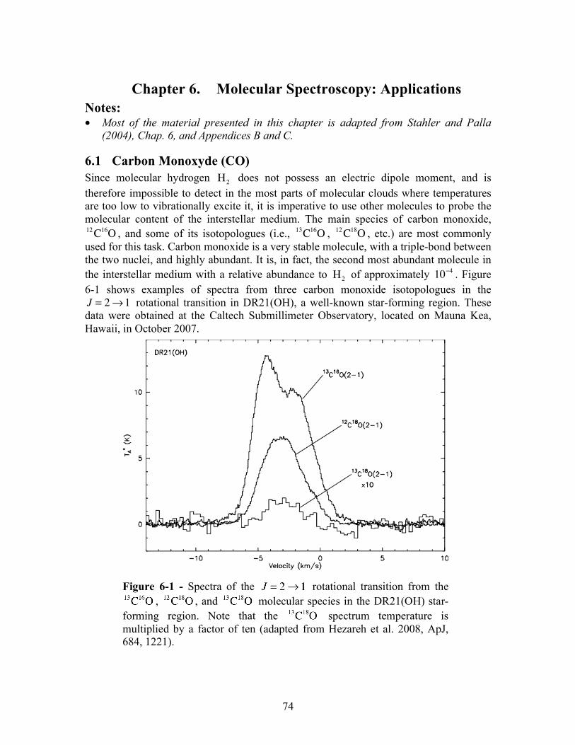
6.1 Carbon Monoxyde (CO) Since molecular hydrogen H2 does not possess an electric dipole moment, and is therefore impossible to detect in the most parts of molecular clouds where temperatures are too low to vibrationally excite it, it is imperative to use other molecules to probe the molecular content of the interstellar medium. The main species of carbon monoxide, 12C16O , and some of its isotopologues (i.e., 13C16O , 12C18O , etc.) are most commonly used for this task. Carbon monoxide is a very stable molecule, with a triple-bond between the two nuclei, and highly abundant. It is, in fact, the second most abundant molecule in the interstellar medium with a relative abundance to H2 of approximately 10−4 . Figure 6-1 shows examples of spectra from three carbon monoxide isotopologues in the J = 2→1 rotational transition in DR21(OH), a well-known star-forming region. These data were obtained at the Caltech Submillimeter Observatory, located on Mauna Kea, Hawaii, in October 2007.

Figure 6-1 - Spectra of the rotational transition from the , , and molecular species in the DR21(OH) star-

forming region. Note that the spectrum temperature is multiplied by a factor of ten (adapted from Hezareh et al. 2008, ApJ, 684, 1221).

75

6.1.1 The Detection Equation We start by revisiting equation (2.25) we previously derived for the specific intensity Iν measured at some location away from an emitting region, of source function Sν , which is also located between the point of observation and some background emission Iν 0( ) . We have shown that Iν = Iν 0( )e−τν + Sν 1− e−τν( ), (6.1) where τν is the optical depth through the emitting region. We will now somewhat refine the treatment we presented in Section 3.1.1 and consider the difference Iν − Iν 0( ) , which we will equate to the intensity of a black body of (brightness) temperature TB in the Rayleigh-Jeans limit

Iν − Iν 0( ) = 2ν2

c2kTB. (6.2)

The reason for considering Iν − Iν 0( ) and not Iν − Iν 0( )e−τν is that usually during an observation the telescope will first be pointed on the source (commonly called ON-position or ON-source), where Iν is measured, and then at a point away for the emitting region on the plane of the sky where only Iν 0( ) is present (OFF-position or OFF-source); this method of observation is often referred to as beam switching. Combining equations (6.1) and (6.2) we have Iν − Iν 0( ) = Sν − Iν 0( )⎡⎣ ⎤⎦ 1− e

−τν( ), (6.3) or

TB =c2

2kν 2 Sν − Iν 0( )⎡⎣ ⎤⎦ 1− e−τν( ). (6.4)

Finally, we further assume that both the source and background intensities can be well approximated by Planck’s blackbody functions of temperature Tex and Tbg , respectively (‘ex’ stands for ‘excitation’). We can therefore write the so-called detection equation as

TB = T01

eT0 Tex −1− 1eT0 Tbg −1

⎛⎝⎜

⎞⎠⎟ 1− e

−τν( ), (6.5)

where T0 ≡ hν k is the equivalent temperature of the transition responsible for the detected radiation.

76

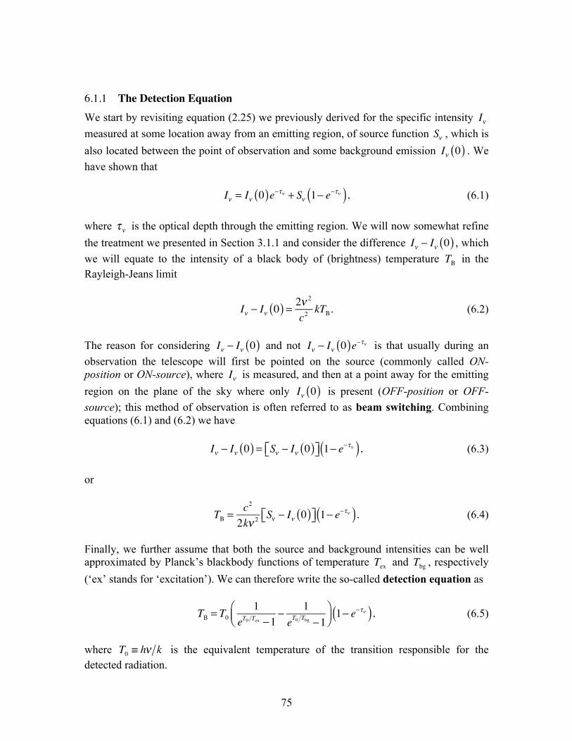
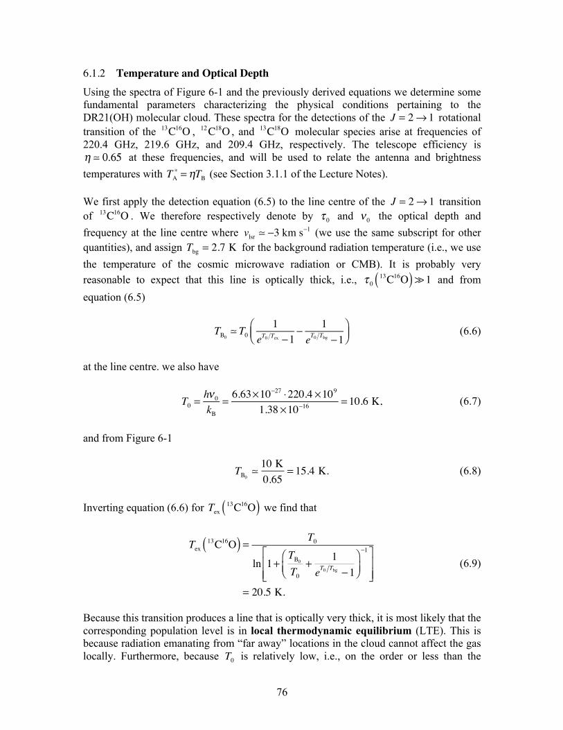
6.1.2 Temperature and Optical Depth Using the spectra of Figure 6-1 and the previously derived equations we determine some fundamental parameters characterizing the physical conditions pertaining to the DR21(OH) molecular cloud. These spectra for the detections of the J = 2→ 1 rotational transition of the 13C16O , 12C18O , and 13C18O molecular species arise at frequencies of 220.4 GHz, 219.6 GHz, and 209.4 GHz, respectively. The telescope efficiency is η 0.65 at these frequencies, and will be used to relate the antenna and brightness temperatures with TA

∗ =ηTB (see Section 3.1.1 of the Lecture Notes). We first apply the detection equation (6.5) to the line centre of the J = 2→ 1 transition of 13C16O . We therefore respectively denote by τ 0 and ν0 the optical depth and frequency at the line centre where vlsr −3 km s−1 (we use the same subscript for other quantities), and assign Tbg = 2.7 K for the background radiation temperature (i.e., we use the temperature of the cosmic microwave radiation or CMB). It is probably very reasonable to expect that this line is optically thick, i.e.,

τ 0

13C16O( )1 and from equation (6.5)

TB0 T0

1eT0 Tex −1

− 1eT0 Tbg −1

⎛⎝⎜

⎞⎠⎟ (6.6)

at the line centre. we also have

T0 =hν0

kB

= 6.63×10−27 ⋅220.4 ×109

1.38 ×10−16 = 10.6 K, (6.7)

and from Figure 6-1

TB0

10 K0.65

= 15.4 K. (6.8)

Inverting equation (6.6) for Tex

13C16O( ) we find that

Tex13C16O( ) = T0

ln 1+TB0

T0

+ 1eT0 Tbg −1

⎛⎝⎜

⎞⎠⎟

−1⎡

⎣⎢⎢

⎤

⎦⎥⎥

= 20.5 K.

(6.9)

Because this transition produces a line that is optically very thick, it is most likely that the corresponding population level is in local thermodynamic equilibrium (LTE). This is because radiation emanating from “far away” locations in the cloud cannot affect the gas locally. Furthermore, because T0 is relatively low, i.e., on the order or less than the

77

expected gas temperature in a molecular cloud, the energy levels involved in this transition can easily be excited through collisions within the gas, and Tex

13C16O( ) is therefore at a level that is perfectly suited for the kinetic temperature of the gas. We then write Tex

13C16O( ) = Tkin . (6.10) Although the corresponding 12C18O transition is not likely to be strongly optically thick, it is to be expected that this molecule will be coexistent with 13C16O and, therefore, subjected to similar physical conditions. Moreover, the J = 2→ 1 transitions for these two molecular species have very similar characteristics (i.e., T0 , ncrit , etc.). We therefore write that Tex

12 C18O( ) = Tkin = 20.5 K. (6.11) We calculate for this transition

T0 =

219.6220.4

⋅10.6 K 10.6 K, (6.12)

and from equation (6.5) we have

τ 0

12C18O( ) = − ln 1−TB0T0

1eT0 Tex −1

− 1eT0 Tbg −1

⎛⎝⎜

⎞⎠⎟−1⎡

⎣⎢

⎤

⎦⎥

= 1.0,

(6.13)

where TB0

= 6.5 K 0.65 = 10 K was used. Since this transition is marginally optically

thin or thick, we should be careful in assuming that isotopologues, such as 12C18O , are unequivocally optically thin, as is too often asserted (see the comment from Stahler and Palla at the beginning of their Section 6.3.1). On the other hand, considering the weakness of the 13C18O line, it is likely that the relation τ 0

13C18O( )1 is satisfied. We also assume that Tex

13C18O( ) = Tkin = 20.5 K, (6.14) for the same reasons as in the case of 12C18O earlier and equation (6.5) then becomes

τ 0 =TB0T0

1eT0 Tex −1

− 1eT0 Tbg −1

⎛⎝⎜

⎞⎠⎟−1

. (6.15)

78

Using

T0 =209.4220.4

⋅10.6 K 10.1 K

TB0= 0.18 K

0.65 0.28 K

(6.16)

we have τ 0 0.02. (6.17) This value is much less than unity and, therefore, consistent with our assumption. We note that the optical depth values obtained for these three transitions are qualitatively consistent with the appearances of their corresponding line profiles shown in Figure 6-1. More precisely, the 13C16O profile is heavily saturated (i.e., flattish) even showing signs of self-absorption (note the ‘dip’ near the line centre), both indications that its optical depth is much larger than unity; the 12C18O profile with

τ 0

12C18O( ) 1 only shows the beginnings of saturation broadening; finally, although it is admittedly more difficult to judge in view of its weakness, the 13C18O line profile shows no obvious sign of saturation.

6.1.3 Transitions between Two Levels and Column Density

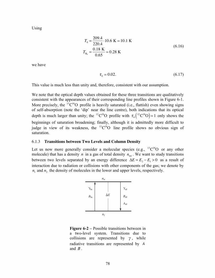
Let us now more generally consider a molecular species (e.g., 13C18O or any other molecule) that has a density n in a gas of total density ntot . We want to study transitions between two levels separated by an energy difference ΔE = E2 − E1 > 0 as a result of interaction due to radiation or collisions with other components of the gas; we denote by n1 and n2 the density of molecules in the lower and upper levels, respectively.

794 B The Two-Level System

drift relative to the background of distant stars. This phenomenon, known as precession of the equinoxes,continually alters the coordinate values for any object. In any particular observation, these values are re-ferred to the appropriate epoch, the current one being the year 2000. Our maps in this book reproduce thecoordinates as published in the literature. The reader who needs a precise location for any object shouldrefer to the original article, as listed in the Sources section, to ascertain the epoch used. Standard programscan, if necessary, shift the coordinate values to the current ones.

In the galactic coordinate system, one places objects with respect to the plane of the Milky Way (seeFigure A.2). This plane intersects the celestial sphere in the Galactic equator, a band that is tilted by 63!

from the celestial one. The longitude (l) of the object is measured eastward along the Galactic equator.Here, the zero point is the Galactic center (open circle in the figure), which is located in the constellationSagittarius, in the Southern hemisphere. For the latitude (b), we measure the angle north or south of theGalactic equator. Both the longitude and latitude are given in degrees, arcminutes, and arcseconds. Apositive b-value indicates that the object is north of the equator. The origin (l = 0; b = 0) corresponds,in equatorial coordinates, to (! = 17h45m37s; " = !28!56"10"").

B The Two-Level System

We consider a species of atom or molecule of number density n dispersed throughout a gas of total den-sity ntot and homogeneous composition. This species has only two energy levels, separated by !E(Figure B.1). In any real system, there are always other levels connected by possible physical transitions.Our two-level approximation is valid to the extent that these other transitions are slow compared to the oneof interest. We include the possibility of degeneracy, i. e., we suppose that there exist gu and gl sublevelsof identical energy in the upper and lower levels, respectively. Our problem is to find the level populationsnu and nl as a function of the ambient kinetic temperature Tkin and density ntot.

As illustrated in the figure, each atom in the lower level can be excited both collisionally and radia-tively. The total rate of collisional excitations per unit time and per unit volume can be written #lu ntot nl,where the coefficient #lu depends on atomic properties of the species of interest and the background gas,as well as on their relative velocity distribution. The probability per unit time of a single atom being ex-cited radiatively must be proportional to the ambient radiation intensity. Thus, we write this probabilityas Blu J̄ nl. Here Blu is the Einstein coefficient for absorption. The quantity J̄ is related to the meanintensity J! by

J̄ "Z #

0

J! $(%) d% (B.1)

Figure B.1 Processes governing the populations in thetwo-level system. These include: collisions with othermolecules, interaction with ambient radiation, and spon-taneous emission.

Figure 6-2 – Possible transitions between in a two-level system. Transitions due to collisions are represented by , while radiative transitions are represented by and .

79

Transitions due to collisions are represented by γ 12 and γ 21 , i.e., the total rate of collisional excitation per unit volume is given by γ 12n1ntot , etc. Transitions due to radiative processes are characterized by the Einstein coefficients B12 , B21 , and A21 . The rate of radiative excitation per unit volume from absorption is B12n1J , the corresponding rate for the emission of photons from stimulated emission is B21n2J , while the rate of spontaneous emission is A21n2 . The quantity J is related to the mean intensity (see eq. (2.19) in Chapter 2) through J = Jνφ ν( )dν

0

∞

∫ , (6.18)

with φ ν( ) the intrinsic line profile. This profile is centered at ν0 = ΔE h and normalized with φ ν( )dν

0

∞

∫ = 1. (6.19)

Under conditions of equilibrium the level populations will remain unchanged with time (in a statistical sense) and we have γ 12n1ntot + B12n1J = γ 21n2ntot + B21n2J + A21n2. (6.20) For cases where collisions dominate ( γ ntot BJ ) we find that

γ 12γ 21

= n2n1, (6.21)

for which, under local thermodynamic equilibrium (LTE) conditions, the right-hand side must obey the Boltzmann distribution at the kinetic temperature Tkin that characterizes the collisions. That is,

γ 12γ 21

= g2g1e−ΔE kTkin . (6.22)

This equation will hold for any conditions. On the other hand, when radiative processes completely dominate ( γ ntot BJ ) the system will come in equilibrium at the radiation temperature Trad and equation (6.20) becomes

J = A21 B21g1B12 g2B21( )eΔE kTkin −1

. (6.23)

80

Since under equilibrium conditions the mean intensity must equal Planck’s blackbody law, i.e., Jν = Bν , we have

J = Bνφ ν( )dν0

∞

∫ Bν φ ν( )dν

0

∞

∫ Bν

(6.24)

because Bν is much broader than φ ν( ) . We therefore write

A21 B21g1B12 g2B21( )eΔE kTrad −1

= 2hν03 c2

eΔE kTrad −1, (6.25)

or

A21 =2hν0

3

c2B21

g1B12 = g2B21. (6.26)

These relations are also valid in general. We now slightly rewrite equation (6.1) with

Iν = Iν 0( )e−τν + jναν

1− e−τν( ), (6.27)

where we used the ratio of the emissivity jν and the absorption coefficient αν = ρκν (i.e., the inverse of the photon mean free path, with κν is the opacity; see Sec. 2.2.2 in Chapter 2) in lieu of the source function Sν . We use the Einstein coefficients to express

jν =

hν4π

n2A21φ ν( )

αν =hν4π

n1B12 − n2B21( )φ ν( ) (6.28)

where it was assumed that the emission is isotropic. It is to be noted that the absorption coefficient contains a correction due to the presence of stimulated emission in the last of equations (6.28). Calculating the ratio jν αν from equations (6.26) and (6.28) would lead us back to equation (6.25) (and to expressing the source function with Planck’s law), as would be expected. We can, however, use our equation for the absorption coefficient

81

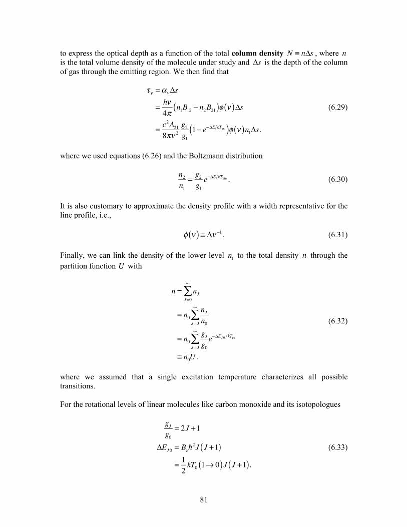
to express the optical depth as a function of the total column density N ≡ nΔs , where n is the total volume density of the molecule under study and Δs is the depth of the column of gas through the emitting region. We then find that

τν =ανΔs

= hν4π

n1B12 − n2B21( )φ ν( )Δs

= c2A218πν 2

g2g11− e−ΔE kTex( )φ ν( )n1Δs,

(6.29)

where we used equations (6.26) and the Boltzmann distribution

n2n1

= g2g1e−ΔE kTkin . (6.30)

It is also customary to approximate the density profile with a width representative for the line profile, i.e., φ ν( ) ≡ Δν−1. (6.31) Finally, we can link the density of the lower level n1 to the total density n through the partition function U with

n = nJJ=0

∞

∑

= n0nJn0J=0

∞

∑

= n0gJg0J=0

∞

∑ e−ΔEJ 0 kTex

≡ n0U.

(6.32)

where we assumed that a single excitation temperature characterizes all possible transitions. For the rotational levels of linear molecules like carbon monoxide and its isotopologues

gJg0

= 2J +1

ΔEJ 0 = Be2J J +1( )

= 12kT0 1→ 0( )J J +1( ).

(6.33)

82

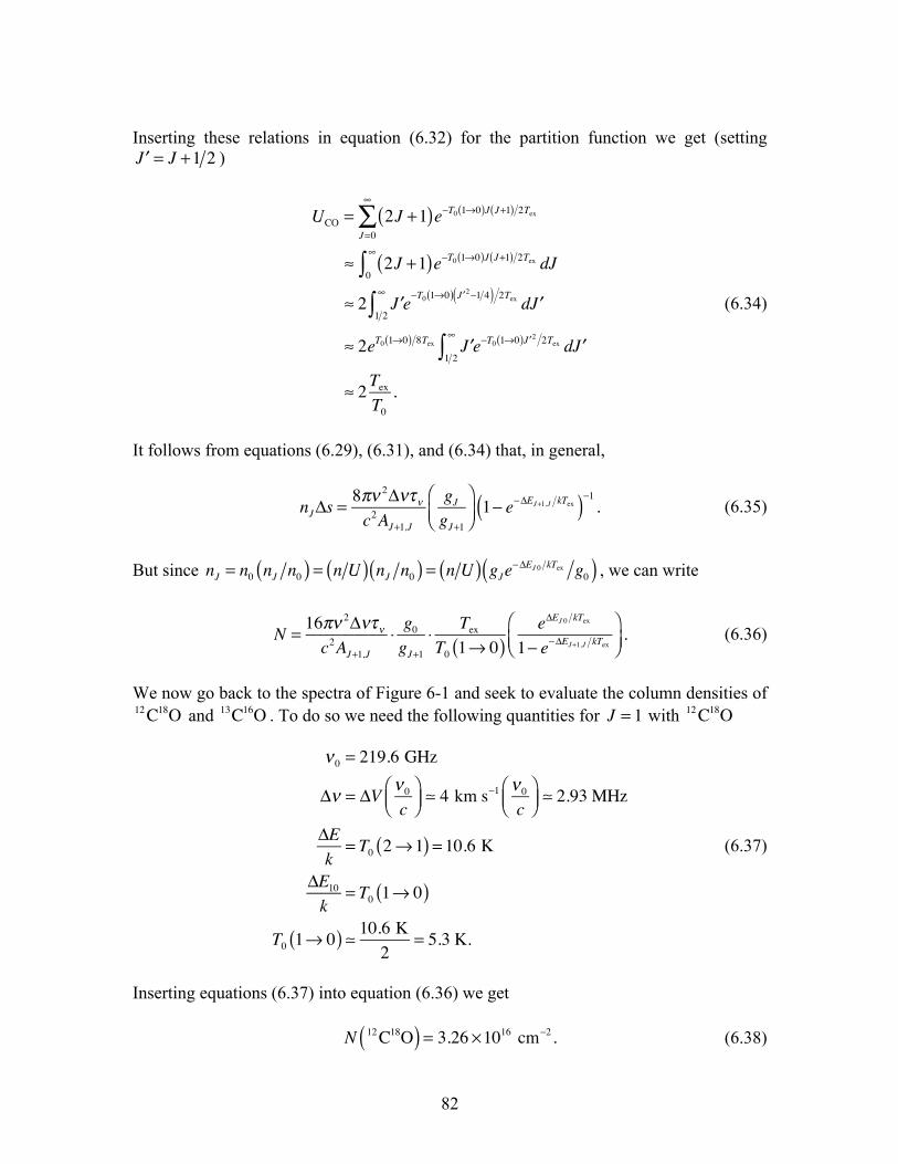
Inserting these relations in equation (6.32) for the partition function we get (setting ′J = J +1 2 )

UCO = 2J +1( )e−T0 1→0( )J J+1( ) 2Tex

J=0

∞

∑

≈ 2J +1( )e−T0 1→0( )J J+1( ) 2Tex dJ0

∞

∫≈ 2 ′J e−T0 1→0( ) ′J 2−1 4( ) 2Tex d ′J

1 2

∞

∫≈ 2eT0 1→0( ) 8Tex ′J e−T0 1→0( ) ′J 2 2Tex d ′J

1 2

∞

∫≈ 2Tex

T0.

(6.34)

It follows from equations (6.29), (6.31), and (6.34) that, in general,

nJΔs =8πν 2Δντν

c2AJ+1,J

gJgJ+1

⎛⎝⎜

⎞⎠⎟1− e−ΔEJ+1,J kTex( )−1 . (6.35)

But since nJ = n0 nJ n0( ) = n U( ) nJ n0( ) = n U( ) gJe−ΔEJ 0 kTex g0( ) , we can write

N = 16πν2Δντν

c2AJ+1,J

⋅ g0gJ+1

⋅ TexT0 1→ 0( )

eΔEJ 0 kTex

1− e−ΔEJ+1,J kTex

⎛⎝⎜

⎞⎠⎟. (6.36)

We now go back to the spectra of Figure 6-1 and seek to evaluate the column densities of 12C18O and 13C16O . To do so we need the following quantities for J = 1 with 12C18O

ν0 = 219.6 GHz

Δν = ΔV ν0

c⎛⎝⎜

⎞⎠⎟ 4 km s−1 ν0

c⎛⎝⎜

⎞⎠⎟ 2.93 MHz

ΔEk

= T0 2→1( ) = 10.6 K

ΔE10

k= T0 1→ 0( )

T0 1→ 0( ) 10.6 K2

= 5.3 K.

(6.37)

Inserting equations (6.37) into equation (6.36) we get N 12 C18O( ) = 3.26 ×1016 cm−2. (6.38)

83

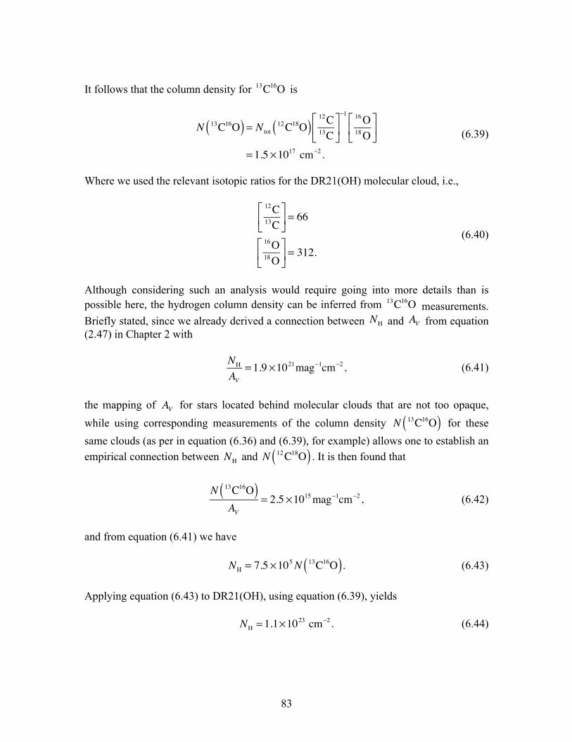
It follows that the column density for 13C16O is

N 13C16O( ) = N tot12 C18O( )

12 C13C

⎡

⎣⎢

⎤

⎦⎥

−1 16 O18 O

⎡

⎣⎢

⎤

⎦⎥

= 1.5 ×1017 cm−2.

(6.39)

Where we used the relevant isotopic ratios for the DR21(OH) molecular cloud, i.e.,

12C13C

⎡

⎣⎢

⎤

⎦⎥ = 66

16O18O

⎡

⎣⎢

⎤

⎦⎥ = 312.

(6.40)

Although considering such an analysis would require going into more details than is possible here, the hydrogen column density can be inferred from 13C16O measurements. Briefly stated, since we already derived a connection between NH and AV from equation (2.47) in Chapter 2 with

NH

AV= 1.9 ×1021mag−1cm−2, (6.41)

the mapping of AV for stars located behind molecular clouds that are not too opaque, while using corresponding measurements of the column density N 13C16O( ) for these same clouds (as per in equation (6.36) and (6.39), for example) allows one to establish an empirical connection between NH and N 12C18O( ) . It is then found that

N 13C16O( )

AV= 2.5 ×1015mag−1cm−2, (6.42)

and from equation (6.41) we have NH = 7.5 ×105N 13C16O( ). (6.43) Applying equation (6.43) to DR21(OH), using equation (6.39), yields NH 1.1×1023 cm−2. (6.44)