49

CHAPTER 3

SIMULATION MODELS FOR MULTICOMPONENT DISTILLATION PROCESS AND REACTIVE DISTILLATION

PROCESS

3.1 INTRODUCTION

The distillation process has very large time constant and it is not economically

feasible to implement a new control strategy on an industrial process. It is

often desirable to test the strategy using dynamic computer simulations of the

process. The mathematical models facilitate the evaluation of alternative

process, tuning of controllers, determining the dynamic effects of

disturbances, optimizing plant operation and investigating potential safety

problems without disturbing the actual process [162]. The simulated models

can also be used to rearrange the manipulated and controlled variable pairing

of the process. Dynamic mathematical models are thus essential, efficient and

powerful tools for simulation study of distillation process. In order to represent

realistic operation of the actual continuous distillation process a rigorous non

linear model is required. Such a model is developed using dynamic material

balance, energy balance and enthalpy equations, supported by vapor liquid

equilibrium and physical properties. Luyben [155] used rigorous models for

design and dynamic control of various reactive distillation systems. The

rigorous models are solved with the help of MATLAB programs or ASPEN

technology simulation software. Several other researchers [48][8][28][80] have

also used the mathematical models, developed in ASPEN software, for

design, modeling, simulation and control of distillation processes.

In the present work, semirigorous mathematical models of multicomponent

distillation process and reactive distillation process are considered for the

analysis and control purposes. As semi rigorous model assumes rapid energy

dynamics, the enthalpy balance thus reduces to an algebraic equation. This

50

means thermal equilibrium is achieved much faster than phase equilibrium.

The detailed mathematical models, modeling assumptions and the simulation

algorithms of these processes are discussed below.

3.2 MATHEMATICAL MODELING OF MULTICOMPONENT DISTILLATION

PROCESS

Distillation is a process of separating feed streams and purifying final and

intermediate product streams by application and removal of heat. A

multicomponent distillation process separates a mixture of more than two

components.

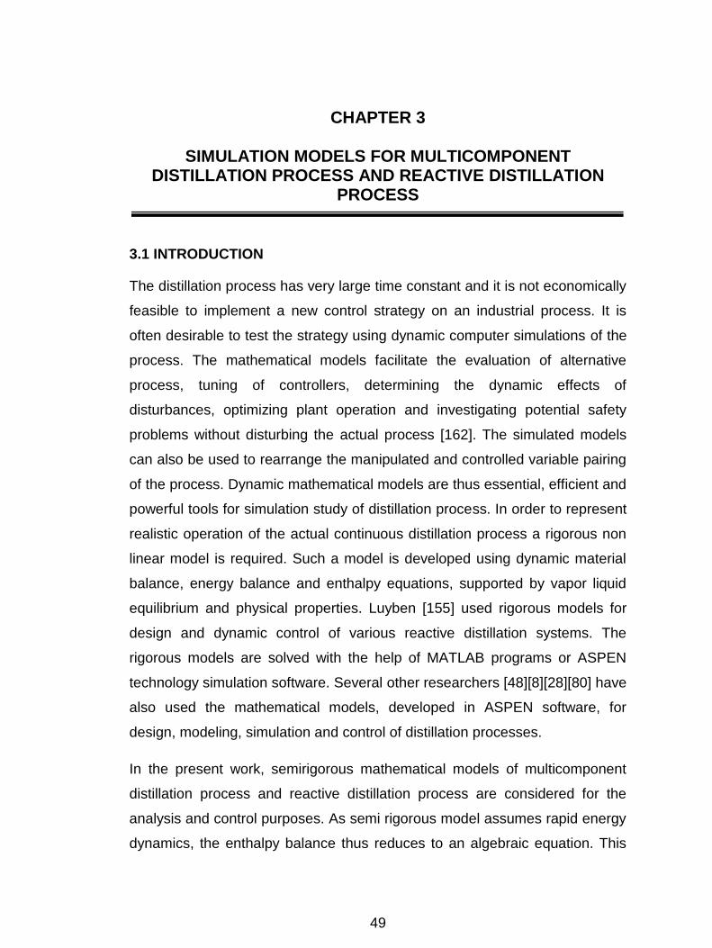
Figure 3.1 Schematic diagram of distillation process with complete details

In the present case a mixture of five components, is separated into its

component fractions using continuous distillation. The process under

NI MODULES INTERNET

SWITCH

REBOILER SUPPLY

CONDENSER

PRESSURE

TRANSDUCERS

FEED TRAYS VERTICAL SHELL

CONTROLLER UNIT PANEL

1

2

NF=5

15

Reflux=400 lb-mol/h

QC

D=200 lb-mol/h

Distillate

XB= [0 7.25 e-03 4.88 e-02 8.36 e-1 1.08 e-1]

VB

3

Condenser

Reflux Drum

Overhead Vapor

Reboiler

Bottoms (B)

QB=5.0 * 106

Btu

Column F=1000 lb-mol/h

ZF

XF YF 0.05 0.40 0.60 0.53 0.01 0.02 0.30 0.05 0.04 0.00

XD= [1.74e-02 9.82 e-01 8.24 e-05 4.93 e-05 6.59 e-10]

]

51

consideration (figure 3.1) is a hypothetical model [156] having 15 trays and 5th

tray is used as the feed tray. The reboiler heat input to the process is

5.275*109 Joule (5.0*106 Btu) and reflux flow rate is 181.6 kg-mol/h (400.0 lb-

mol/h). The liquid and vapor feed rate is 363.2 kg-mol/h (800 lb-mol/h) and

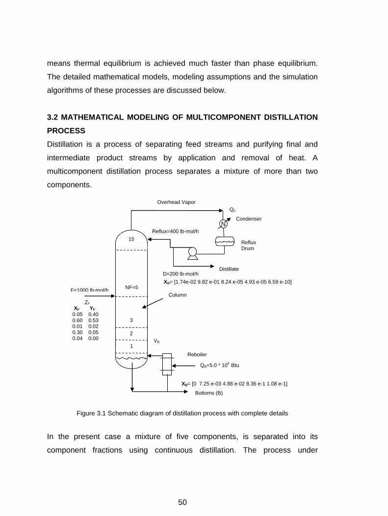
90.8 kg-mol/h (200 lb-mol/h) respectively. The other column and mixture

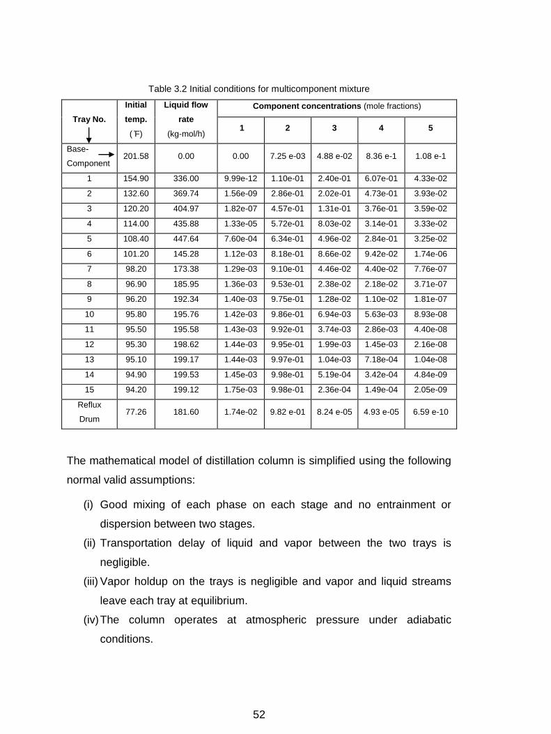
details are given in table 3.1. The initial conditions of the distillation process

are given in table 3.2.

Table 3.1 Column and mixture details for multicomponent mixture

Number of trays NT = 15

Position of feed tray = tray 5

Weir height in stripping section WHS = 0.75 in (0.019m)

Weir length in stripping section WLS = 1.25 in (0.03175m)

Column diameter in stripping section DS = 72 in (1.8288m)

Weir height in rectifying section WHR = 48 in (1.219m)

Weir length in rectifying section WLR = 48 in (1.219m)

Column diameter in rectifying section DS = 72 in (1.8288m)

Number of components = 5

Volumetric hold up in column base = 10.0 ft3 (0.283m

3 )

Volumetric hold up in reflux drum = 10.0 ft3 (0.283 m

3 )

Liquid feed rate FL = 363.2 kg-mol/h (800 lb-mol/h)

Vapor feed rate FV = 90.8 kg-mol/h (200 lb-mol/h)

Liquid feed temperature TFL = 48.88 oC (120 F)

Pressure in the bottom = 146.13 kPa (21.20 psia)

Pressure in the reflux drum = 135.79 kPa (19.7 psia)

Reboiler heat input = 5.275 * 109 Joule (5.0 * 10

6 Btu)

Reflux flow rate = 181.6 kg-mol/h (400.0 lb-mol/h)

Vapor distillate product flow rate = 90.8 kg-mol/h (200.00 lb-mol/h)

Murphree vapors efficiency = 0.5

Component MW DENS HVAP BPT HCAPV HCAPL VP1 T1 VP2 T2

LLK 30.00 40.00 100.0 10.00 0.20 0.60 14.70 10.00 50.00 30.00

LK 50.00 40.00 90.00 90.00 0.40 0.60 14.70 90.00 500.0 200.0

INTER 90.00 60.00 70.00 150.0 0.30 0.50 14.70 150.0 150.0 200.0

HK 130.0 70.00 80.00 210.0 0.30 0.40 14.70 210.0 150.0 300.0

HHK 300.0 90.00 80.00 360.0 0.30 0.40 14.70 360.0 150.0 420.0

52

Table 3.2 Initial conditions for multicomponent mixture

Tray No.

Initial

temp.

( F)

Liquid flow

rate

(kg-mol/h)

Component concentrations (mole fractions)

1 2 3 4 5

Base-

Component 201.58 0.00 0.00 7.25 e-03 4.88 e-02 8.36 e-1 1.08 e-1

1 154.90 336.00 9.99e-12 1.10e-01 2.40e-01 6.07e-01 4.33e-02

2 132.60 369.74 1.56e-09 2.86e-01 2.02e-01 4.73e-01 3.93e-02

3 120.20 404.97 1.82e-07 4.57e-01 1.31e-01 3.76e-01 3.59e-02

4 114.00 435.88 1.33e-05 5.72e-01 8.03e-02 3.14e-01 3.33e-02

5 108.40 447.64 7.60e-04 6.34e-01 4.96e-02 2.84e-01 3.25e-02

6 101.20 145.28 1.12e-03 8.18e-01 8.66e-02 9.42e-02 1.74e-06

7 98.20 173.38 1.29e-03 9.10e-01 4.46e-02 4.40e-02 7.76e-07

8 96.90 185.95 1.36e-03 9.53e-01 2.38e-02 2.18e-02 3.71e-07

9 96.20 192.34 1.40e-03 9.75e-01 1.28e-02 1.10e-02 1.81e-07

10 95.80 195.76 1.42e-03 9.86e-01 6.94e-03 5.63e-03 8.93e-08

11 95.50 195.58 1.43e-03 9.92e-01 3.74e-03 2.86e-03 4.40e-08

12 95.30 198.62 1.44e-03 9.95e-01 1.99e-03 1.45e-03 2.16e-08

13 95.10 199.17 1.44e-03 9.97e-01 1.04e-03 7.18e-04 1.04e-08

14 94.90 199.53 1.45e-03 9.98e-01 5.19e-04 3.42e-04 4.84e-09

15 94.20 199.12 1.75e-03 9.98e-01 2.36e-04 1.49e-04 2.05e-09

Reflux

Drum 77.26 181.60 1.74e-02 9.82 e-01 8.24 e-05 4.93 e-05 6.59 e-10

The mathematical model of distillation column is simplified using the following

normal valid assumptions:

(i) Good mixing of each phase on each stage and no entrainment or

dispersion between two stages.

(ii) Transportation delay of liquid and vapor between the two trays is

negligible.

(iii) Vapor holdup on the trays is negligible and vapor and liquid streams

leave each tray at equilibrium.

(iv) The column operates at atmospheric pressure under adiabatic

conditions.

53

(v) Murphree stage efficiency based on vapor phase is valid.

(vi) A total condenser and a partial reboiler are assumed to be used. The

reflux drum and reboiler holdups are considered to be well-mixed

pools.

(vii) Metal walls and trays have negligible heat capacity i.e. enthalpy of

metal is considered to be negligible.

(viii) There is a definite relationship between the concentration of a

component in the vapor and liquid leaving each tray and is given by

bubble point calculation.

The mass and energy balance equations are derived by applying

conservation laws to each tray, reboiler and condenser.

3.2.1 Component Material Balance Equations

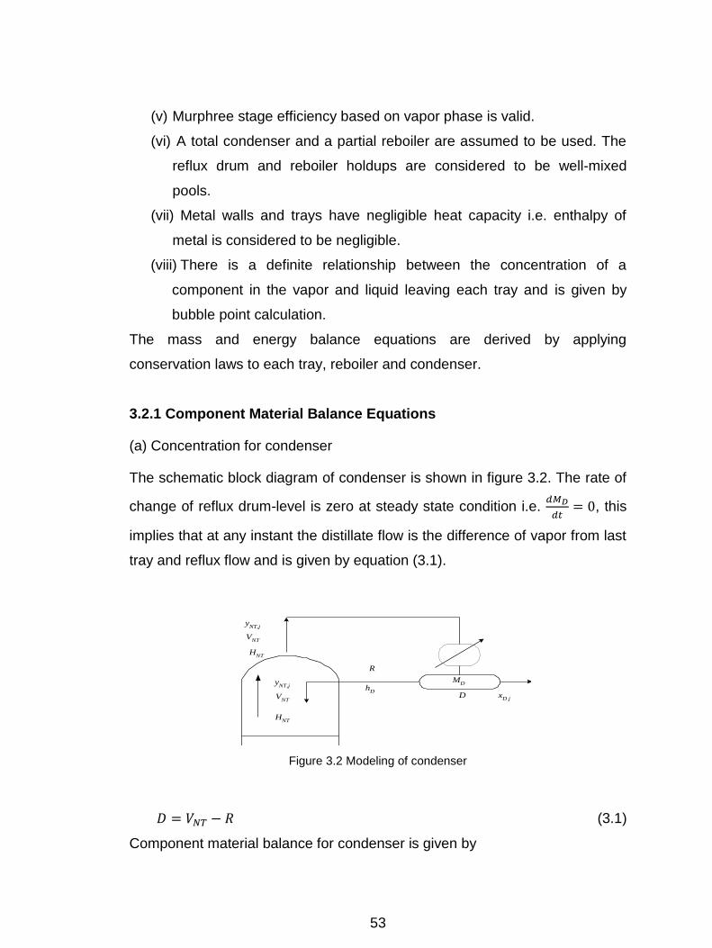
(a) Concentration for condenser

The schematic block diagram of condenser is shown in figure 3.2. The rate of

change of reflux drum-level is zero at steady state condition i.e.

, this

implies that at any instant the distillate flow is the difference of vapor from last

tray and reflux flow and is given by equation (3.1).

D

yNT,j

VNT

HNT

R

hD

xD j

MDy

NT,j

HNT

VNT

Figure 3.2 Modeling of condenser

(3.1)

Component material balance for condenser is given by

54

for (3.2)

where

= No. of trays

= No. of components

= Liquid molar holdup in the reflux drum, lb-mol

= Distillate flow rate, lb-mol/h

= Liquid fraction of component in reflux drum, %mole fraction

= Vapor fraction of component leaving tray , %mole fraction

= Total liquid flow rate entering the tray from reflux drum, lb-mol/h

= Total vapor flow rate leaving the tray , lb-mol/h

(b) Component material balance equation for tray i

The schematic block diagram of general tray is shown in figure 3.3 and the

component material balance for tray is given by

Mi

Vi

yi,j

Hi

Li+1

xi+1,j

hi+1

hFi

Fi

xFi

Vi-1

Hi-1

yi-1,j

Li

xi,j

hi

Figure 3.3 Modeling of general tray i

(3.3)

for

where

= Molar liquid holdup on tray , lb-mol

= Liquid fraction of component leaving the tray , %mole fraction

= Total liquid flow rate leaving tray , lb-mol/h

55

= Total vapor flow rate leaving tray , lb-mol/h

= Total feed flow rate injected to tray , lb-mol/h

= Liquid fraction of component in feed on tray , %mole fraction

The vapor composition of component on tray is obtained as

(3.4)

where

Murphree stage efficiency based on vapor phase of component

on tray

Equilibrium vapor fraction of component on tray

is liquid flow rate on tray is related to molar holdup through the

relationship given below.

(3.5)

where

= Length of the weir, ft

= Net area of the tray, ft2

= Height of the weir, ft

= Average molar density of liquid on tray , lb-mol/ft3

= Liquid flow rate from tray , lb-mol/h

(c) Component material balance equation for reboiler

The schematic diagram of reboiler is shown in figure 3.4. The rate of change

of reboiler holdup is zero at steady state condition i.e.

, that is, at any

instant t, the bottom product rate will be the difference of liquid entering from

first tray and vapor leaving the reboiler and is given by

(3.6)

Component material balance for reboiler is given by

for (3.7)

56

where

= Liquid molar holdup in reboiler, lb-mol

= Total liquid flow rate from tray 1 entering to reboiler, lb-mol/h

= Liquid fraction of component in bottom product, %mole fraction

= Total vapor flow rate leaving reboiler, lb-mol/h

= Vapor fraction of component leaving reboiler, %mole fraction

= Total bottom product rate, lb-mol/h

Tray-1

L1 , x

1,j

Reboiler

VB, y

B,j

MB

h1

QB

B , hB, x

B,j

HB

Figure 3.4 Modeling of reboiler

The vapor fraction of component from reboiler is given by

(3.8)

where

Vaporization efficiency of component in reboiler

Equilibrium constant of component in reboiler

3.2.2 Total Material Balance Equations

The total material balance for general tray i is calculated as

for (3.9)

where

= Total molar holdup on tray , lb-mol

= Total liquid flow rate leaving tray , lb-mol/h

= Total liquid flow rate entering tray , lb-mol/h

57

= Total vapor flow rate leaving tray , lb-mol/h

= Total vapor flow rate entering tray , lb-mol/h

= Total feed flow injected on tray , lb-mol/h

3.2.3 Total Enthalpy Balance Equations

(a) Enthalpy balance for condenser

The enthalpy is defined as the total internal energy and is given by the

product of pressure and volume. The energy dynamics is assumed to be so

rapid that the enthalpy balance reduces to an algebraic equation. This means

that thermal equilibrium is attained much faster than phase equilibrium. Using

the definition, the enthalpy balance for condenser is given by

(3.10)

where

= Total molar enthalpy of vapor leaving the last tray, kJ/lb-mol

= Total molar enthalpy of liquid leaving the reflux drum, kJ/lb-mol

= Condenser duty, kW

(b) Enthalpy balance for general tray i

The enthalpy balance for general tray i is given by the following equation.

(3.11)

for

where

Total molar enthalpy of liquid leaving tray , kJ/lb-mol

Total molar enthalpy of vapor leaving tray , kJ/lb-mol

(c) Enthalpy balance for reboiler

The enthalpy balance for reboiler is given by the equation given below.

(3.12)

where

58

Reboiler duty, Btu/h

Total molar enthalpy of liquid leaving reboiler, kJ/lb-mol

Total molar enthalpy of vapor leaving reboiler, kJ/lb-mol

Enthalpies of liquid and vapor on tray are calculated by mixing rule and are

given by

(3.13)

(3.14)

where and represent pure component enthalpies of component on

tray in liquid and vapor phase respectively.

A tray is said to be in equilibrium, when the tray temperature satisfy bubble

point relation, and calculated using equations (3.15a), (3.15b) and (3.15c) as

follows. Using Raoult’s law the component vapor pressure is given by

(3.15a)

where

= Vapor pressure of component on tray , kPa

= Constants for component on tray

Tray temperature of be calculated, F

The vapor fraction is related to liquid fraction using component vapor pressure

and total pressure by following equation.

(3.15b)

where

= Total vapor pressure on tray , kPa

= Liquid fraction of component on tray , %mole fraction

(3.15c)

where

= Vapor fraction of component on tray , %mole fraction

The bubble point relationship is satisfied by an iterative procedure.

59

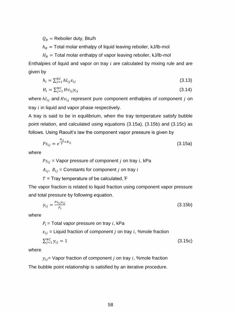
3.3 SIMULATION FLOWCHART FOR MULTICOMPONENT DISTILLATION

PROCESS

The simulation flowchart is developed using the previously listed assumptions.

Figure 3.5 Simulation flowchart for multicomponent distillation process

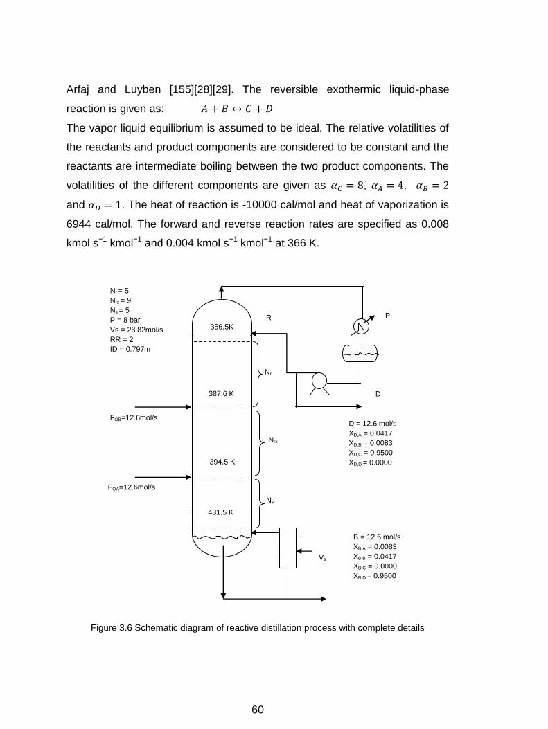
3.4 MATHEMATICAL MODELING FOR REACTIVE DISTILLATION

PROCESS

Reactive distillation column under consideration is a hypothetical two-

reactant-two-product reactive distillation column (figure 3.6) proposed by Al-

NI MODULES INTERNET

SWITCH

REBOILER SUPPLY

CONDENSER

PRESSURE

TRANSDUCERS

FEED TRAYS VERTICAL SHELL

CONTROLLER UNIT PANEL

Input Data (column size, components, physical properties, feeds etc.)

Evaluate initial tray holdup and pressure profile

Calculate temperature profile and vapor fraction

Vapor flow rate on all trays are calculated

Compute derivatives of component continuity equations

Integrate all ODE’s

Evaluate new liquid flow rates and hold up, mole fraction of

components

60

Arfaj and Luyben [155][28][29]. The reversible exothermic liquid-phase

reaction is given as:

The vapor liquid equilibrium is assumed to be ideal. The relative volatilities of

the reactants and product components are considered to be constant and the

reactants are intermediate boiling between the two product components. The

volatilities of the different components are given as , ,

and . The heat of reaction is -10000 cal/mol and heat of vaporization is

6944 cal/mol. The forward and reverse reaction rates are specified as 0.008

kmol s−1 kmol−1 and 0.004 kmol s−1 kmol−1 at 366 K.

Figure 3.6 Schematic diagram of reactive distillation process with complete details

431.5 K

394.5 K

387.6 K

356.5K

Ns

Nrx

Nr

R P

D

FOB=12.6mol/s

FOA=12.6mol/s

Vs

Nr = 5

Nrx = 9

Ns = 5

P = 8 bar

Vs = 28.82mol/s

RR = 2

ID = 0.797m

D = 12.6 mol/s

XD,A = 0.0417

XD,B = 0.0083

XD,C = 0.9500

XD,D = 0.0000

B = 12.6 mol/s

XB,A = 0.0083

XB,B = 0.0417

XB,C = 0.0000

XB,D = 0.9500

61

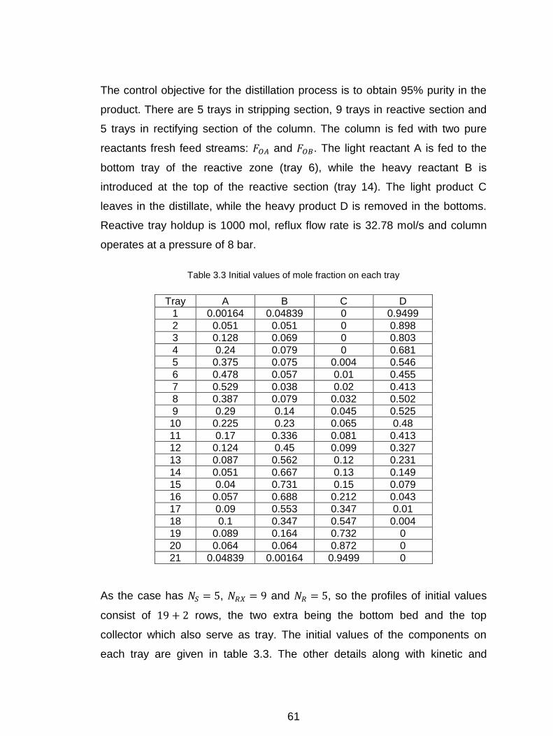
The control objective for the distillation process is to obtain 95% purity in the

product. There are 5 trays in stripping section, 9 trays in reactive section and

5 trays in rectifying section of the column. The column is fed with two pure

reactants fresh feed streams: and . The light reactant A is fed to the

bottom tray of the reactive zone (tray 6), while the heavy reactant B is

introduced at the top of the reactive section (tray 14). The light product C

leaves in the distillate, while the heavy product D is removed in the bottoms.

Reactive tray holdup is 1000 mol, reflux flow rate is 32.78 mol/s and column

operates at a pressure of 8 bar.

Table 3.3 Initial values of mole fraction on each tray

Tray A B C D

1 0.00164 0.04839 0 0.9499

2 0.051 0.051 0 0.898

3 0.128 0.069 0 0.803

4 0.24 0.079 0 0.681

5 0.375 0.075 0.004 0.546

6 0.478 0.057 0.01 0.455

7 0.529 0.038 0.02 0.413

8 0.387 0.079 0.032 0.502

9 0.29 0.14 0.045 0.525

10 0.225 0.23 0.065 0.48

11 0.17 0.336 0.081 0.413

12 0.124 0.45 0.099 0.327

13 0.087 0.562 0.12 0.231

14 0.051 0.667 0.13 0.149

15 0.04 0.731 0.15 0.079

16 0.057 0.688 0.212 0.043

17 0.09 0.553 0.347 0.01

18 0.1 0.347 0.547 0.004

19 0.089 0.164 0.732 0

20 0.064 0.064 0.872 0

21 0.04839 0.00164 0.9499 0

As the case has , and , so the profiles of initial values

consist of rows, the two extra being the bottom bed and the top

collector which also serve as tray. The initial values of the components on

each tray are given in table 3.3. The other details along with kinetic and

62

physical properties and vapour-liquid equilibrium parameters are given in

table 3.4 to table 3.6.

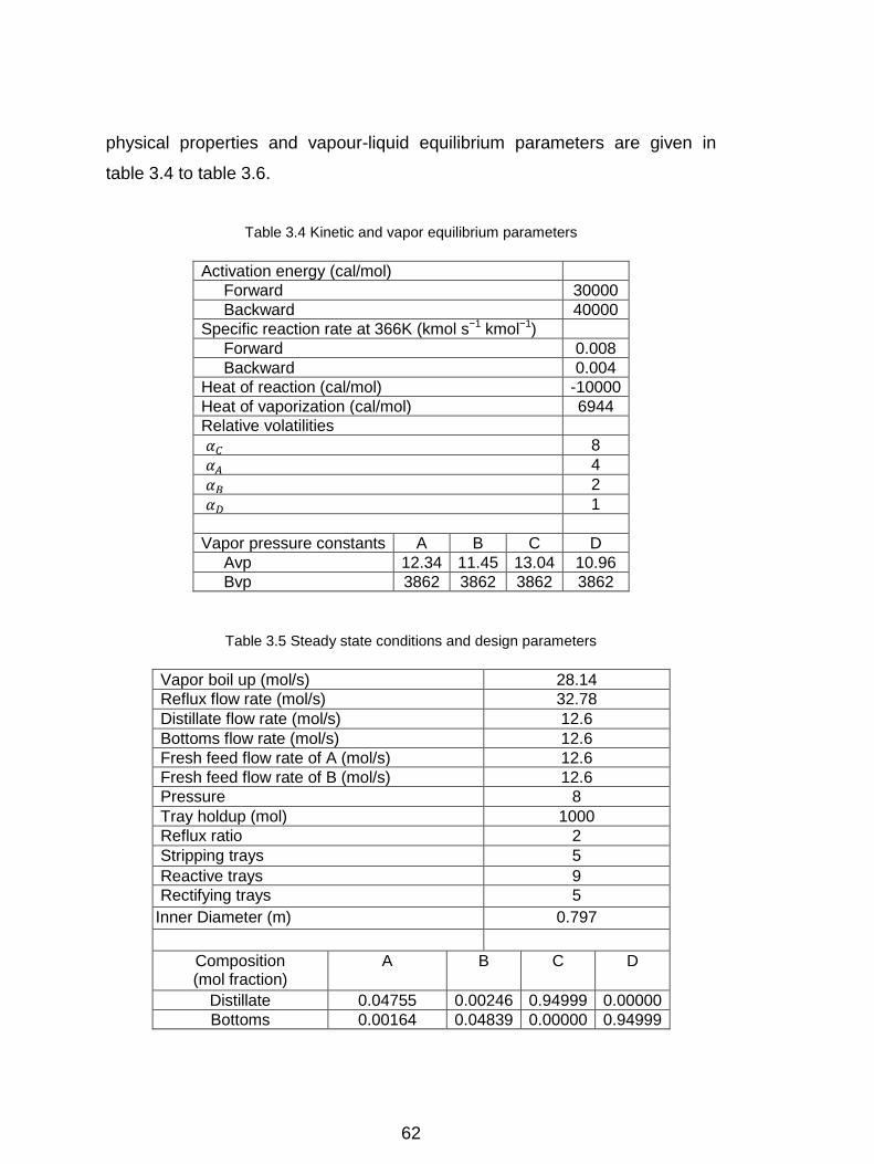
Table 3.4 Kinetic and vapor equilibrium parameters

Activation energy (cal/mol)

Forward 30000

Backward 40000

Specific reaction rate at 366K (kmol s−1 kmol−1)

Forward 0.008

Backward 0.004

Heat of reaction (cal/mol) -10000

Heat of vaporization (cal/mol) 6944

Relative volatilities

8

4

2

1

Vapor pressure constants A B C D

Avp 12.34 11.45 13.04 10.96

Bvp 3862 3862 3862 3862

Table 3.5 Steady state conditions and design parameters

Vapor boil up (mol/s) 28.14 Reflux flow rate (mol/s) 32.78 Distillate flow rate (mol/s) 12.6 Bottoms flow rate (mol/s) 12.6 Fresh feed flow rate of A (mol/s) 12.6 Fresh feed flow rate of B (mol/s) 12.6 Pressure 8 Tray holdup (mol) 1000 Reflux ratio 2 Stripping trays 5 Reactive trays 9 Rectifying trays 5

Inner Diameter (m) 0.797

Composition (mol fraction)

A

B

C D

Distillate 0.04755 0.00246 0.94999 0.00000 Bottoms 0.00164 0.04839 0.00000 0.94999

63

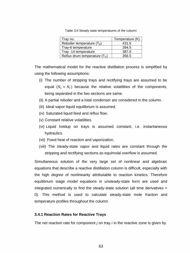
Table 3.6 Steady state temperatures of the column

Tray no. Temperature (K)

Reboiler temperature (TB) 431.5

Tray-6 temperature 394.5

Tray -14 temperature 387.6

Reflux drum temperature (TD) 356.5

The mathematical model for the reactive distillation process is simplified by

using the following assumptions:

(i) The number of stripping trays and rectifying trays are assumed to be

equal ( because the relative volatilities of the components,

being separated in the two sections are same.

(ii) A partial reboiler and a total condenser are considered in the column.

(iii) Ideal vapor-liquid equilibrium is assumed.

(iv) Saturated liquid feed and reflux flow.

(v) Constant relative volatilities.

(vi) Liquid holdup on trays is assumed constant, i.e. instantaneous

hydraulics.

(vii) Fixed heat of reaction and vaporization.

(viii) The steady-state vapor and liquid rates are constant through the

stripping and rectifying sections as equimolal overflow is assumed.

Simultaneous solution of the very large set of nonlinear and algebraic

equations that describe a reactive distillation column is difficult, especially with

the high degree of nonlinearity attributable to reaction kinetics. Therefore

equilibrium stage model equations in unsteady-state form are used and

integrated numerically to find the steady-state solution (all time derivatives =

0). This method is used to calculate steady-state mole fraction and

temperature profiles throughout the column.

3.4.1 Reaction Rates for Reactive Trays

The net reaction rate for component j on tray i in the reactive zone is given by

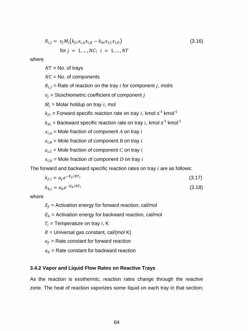
64

(3.16)

for

where

= No. of trays

= No. of components

= Rate of reaction on the tray for component , mol/s

= Stoichiometric coefficient of component

= Molar holdup on tray , mol

= Forward specific reaction rate on tray , kmol s-1 kmol-1

= Backward specific reaction rate on tray , kmol s-1 kmol-1

= Mole fraction of component A on tray

= Mole fraction of component B on tray

= Mole fraction of component C on tray

= Mole fraction of component D on tray

The forward and backward specific reaction rates on tray are as follows:

(3.17)

(3.18)

where

= Activation energy for forward reaction, cal/mol

= Activation energy for backward reaction, cal/mol

= Temperature on tray i, K

= Universal gas constant, cal/(mol K)

= Rate constant for forward reaction

= Rate constant for backward reaction

3.4.2 Vapor and Liquid Flow Rates on Reactive Trays

As the reaction is exothermic, reaction rates change through the reactive

zone. The heat of reaction vaporizes some liquid on each tray in that section;

65

therefore, the vapor rate increases up through the reactive trays and the liquid

rate decreases down through the reactive trays.

for (3.19)

for (3.20)

where

= Vapor flow rate at tray , mol/s

= Liquid flow rate at tray , mol/s

= Heat of vaporization, cal/mol

= Heat of reaction, cal/mol

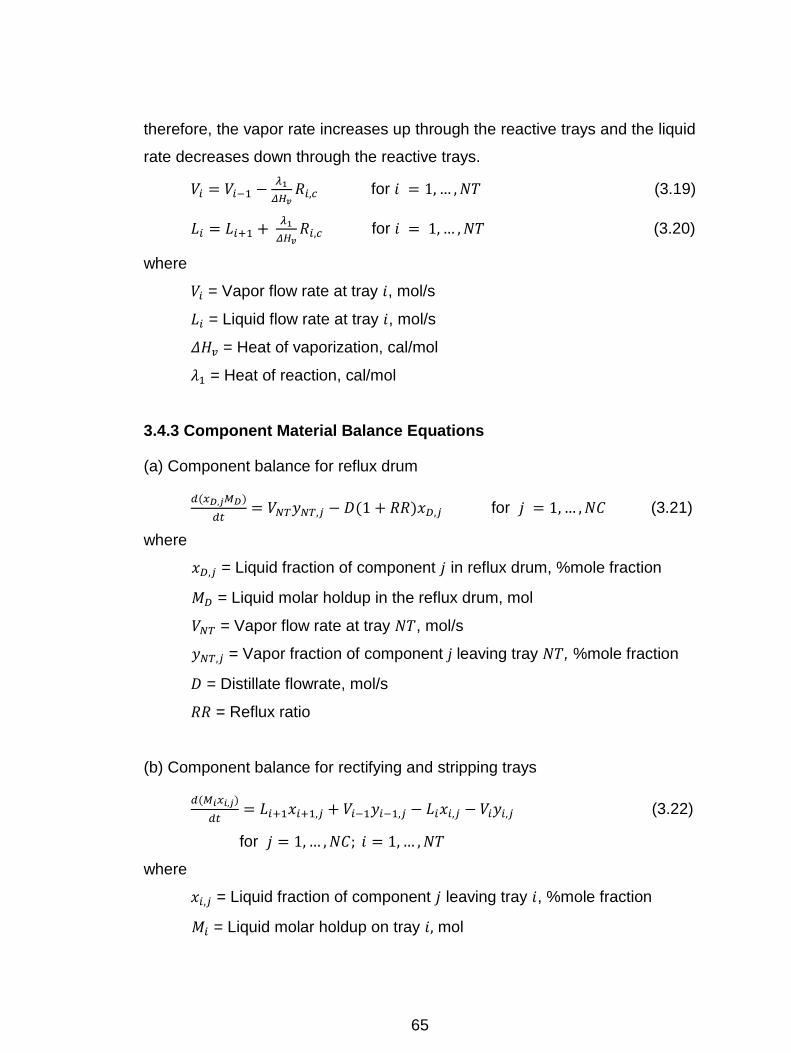
3.4.3 Component Material Balance Equations

(a) Component balance for reflux drum

for (3.21)

where

= Liquid fraction of component in reflux drum, %mole fraction

= Liquid molar holdup in the reflux drum, mol

= Vapor flow rate at tray , mol/s

= Vapor fraction of component j leaving tray , %mole fraction

= Distillate flowrate, mol/s

= Reflux ratio

(b) Component balance for rectifying and stripping trays

(3.22)

for

where

= Liquid fraction of component leaving tray , %mole fraction

= Liquid molar holdup on tray mol

66

= Liquid flow rate leaving tray , mol/s

= Vapor flow rate leaving tray , mol/s

Vapor fraction of component leaving tray , %mole fraction

(c) Component balance for reactive trays

(3.23)

(d) Component balance for feed trays

(3.24)

where

= Input feed flow rate on feed tray , mol/s

= Liquid fraction of component in feed on tray , % mole fraction

(e) Component balance for column base

(3.25)

where

= Liquid molar holdup in reboiler, mol

= Total liquid flow rate from tray 1 entering to reboiler, mol/s

= Liquid fraction of component in bottom product, %mole fraction

= Total vapor flow rate leaving reboiler, mol/s

= Vapor fraction of component leaving reboiler, %mole fraction

= Bottom flow rate, mol/s

3.4.4 Temperature on Tray :

(3.26)

where

= Antione constant for component

67

= Antione constant for component

= Pressure in the column, bar

= Relative volatility for component

With the equimolal overflow mentioned above, the vapor flow rates in the

stripping section are equal to and liquid rates equal to . Analogously,

and are the vapor flow rates and liquid flow rates respectively in rectifying

section. With pressure and tray liquid composition known at each point

in time on each tray, the temperature and the vapor composition can be

calculated. This bubble point calculation can be solved by a Newton-Raphson

iterative convergence method.

(3.27)

(3.28)

where

= Pure vapor pressure of component

Liquid fraction of component leaving tray , %mole fraction

Vapor fraction of component leaving tray , %mole fraction

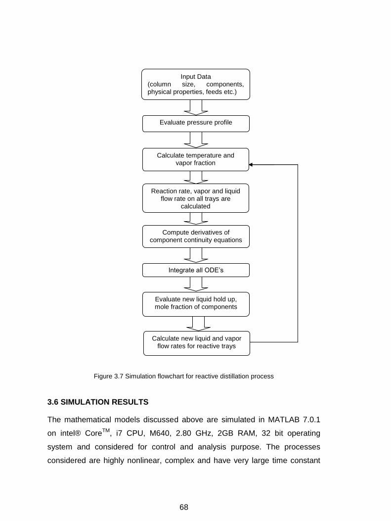
3.5 SIMULATION FLOWCHART FOR REACTIVE DISTILLATION

PROCESS

The simulation flowchart for reactive distillation process is given below.

68

Figure 3.7 Simulation flowchart for reactive distillation process

3.6 SIMULATION RESULTS

The mathematical models discussed above are simulated in MATLAB 7.0.1

on intel® CoreTM, i7 CPU, M640, 2.80 GHz, 2GB RAM, 32 bit operating

system and considered for control and analysis purpose. The processes

considered are highly nonlinear, complex and have very large time constant

NI MODULES INTERNET

SWITCH

REBOILER SUPPLY

CONDENSER

PRESSURE

TRANSDUCERS

FEED TRAYS VERTICAL SHELL

CONTROLLER UNIT PANEL

Input Data (column size, components, physical properties, feeds etc.)

Evaluate pressure profile

Calculate temperature and vapor fraction

Reaction rate, vapor and liquid flow rate on all trays are

calculated

Compute derivatives of component continuity equations

Integrate all ODE’s

Evaluate new liquid hold up, mole fraction of components

Calculate new liquid and vapor flow rates for reactive trays

69

(generally in minutes). As the time constant of distillation process is large, a

fast and efficient controller is needed so that the overall time constant of the

system is not reduced further. The time shown in the results (in seconds) is

the time taken by PC for simulation. A second in the simulation may be

considered nearly equivalent to minutes in a real time process.

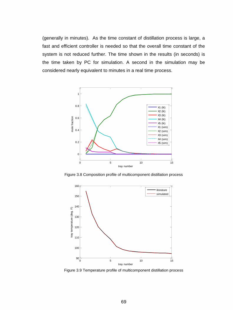
Figure 3.8 Composition profile of multicomponent distillation process

Figure 3.9 Temperature profile of multicomponent distillation process

0 5 10 15

0

0.2

0.4

0.6

0.8

1

tray number

mole

fra

ction

X1 (lit)

X2 (lit)

X3 (lit)

X4 (lit)

X5 (lit)

X1 (sim)

X2 (sim)

X3 (sim)

X4 (sim)

X5 (sim)

0 5 10 1590

100

110

120

130

140

150

160

tray number

tray t

em

pera

ture

(deg.

F)

literature

simulated

70

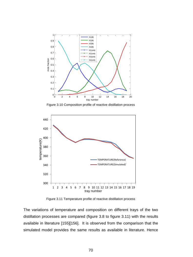
Figure 3.10 Composition profile of reactive distillation process

Figure 3.11 Temperature profile of reactive distillation process

The variations of temperature and composition on different trays of the two

distillation processes are compared (figure 3.8 to figure 3.11) with the results

available in literature [155][156]. It is observed from the comparison that the

simulated model provides the same results as available in literature. Hence

0 2 4 6 8 10 12 14 16 18 200

0.1

0.2

0.3

0.4

0.5

0.6

0.7

0.8

0.9

1

tray number

mole

fra

ction

X1(lit)

X2(lit)

X3(lit)

X4(lit)

X1(sim)

X2(sim)

X3(sim)

X4(sim)

300

320

340

360

380

400

420

440

1 2 3 4 5 6 7 8 9 10 11 12 13 14 15 16 17 18 19

tem

pera

ture

(K)

tray number

TEMPERATURE(Reference)

TEMPERATURE(Simulated)'

71

the process models are validated. The results also show that component X2 is

obtained in distillate and X4 is obtained in bottom in case of multi component

distillation process. In the reactive distillation process X3 (component C) is

obtained in distillate and X4 (component D) is obtained in bottom. The

simulation data thus obtained is used by soft sensors to model the input-

output behavior of the system. It is also found that the composition and

temperature profiles of the two processes are highly nonlinear. Hence there is

a need of highly robust and efficient controllers to achieve the desired control

objective.

3.7 CONCLUSION

The present work uses the semirigorous models of the distillation processes.

The mathematical models of the processes are simulated in MATLAB and the

dynamic issue of the distillation process is also discussed. The developed

models are validated against the results available in literature. The artificial

intelligent techniques are used in the composition measurements as well as

control of distillation processes, the results obtained are discussed in the next

chapter.

NI MODULES INTERNET

SWITCH

REBOILER SUPPLY

CONDENSER

PRESSURE

TRANSDUCERS

FEED TRAYS VERTICAL SHELL

CONTROLLER UNIT PANEL

72