Chapter 15 Multiple Integration - Rowan Universityusers.rowan.edu/~hassen/Mathematica/Volume III/Chapter 15.pdfChapter 15 Multiple Integration Useful Tip: If you are reading the electronic

Chapter 15 Multiple IntegrationUseful Tip: If you are reading the electronic version of this publication formatted as a Mathematica Notebook, then it is possibleto view 3-D plots generated by Mathematica from different perspectives. First, place your screen cursor over the plot. Then dragthe mouse while pressing down on the left mouse button to rotate the plot.

ü 15.1 Double Integral over a Rectangle

Students should read Section 15.1 of Rogawski's Calculus [1] for a detailed discussion of the material presented in thissection.

Integration can be generalized to functions of two or more variables. As the integral of a single-variable function defines area ofa plane region under the curve, it is natural to consider a double integral of a two-variable function that defines volume of a solidunder a surface. This definition can be made precise in terms of double Riemann sums where rectangular columns (as opposed torectangles) are used as building blocks to approximate volume (as opposed to area). The exact volume is then obtained as a limitwhere the number of columns increases without bound.

ü 15.1.1 Double Integrals and Riemann Sums

Let f x, y be a function of two variables defined on a rectangular domain R = a, bä c, d in R2. LetP = a = x0 < x1 < ... < xm = b, c = y0 < y1 < ... < yn = d be an arbitrary partition of R into a grid of m ÿn rectangles, where m and

n are integers. For each sub-rectangle Rij = xi-1, xiä y j-1, y j denote by DAij its area and choose an arbitrary base point

xij, yij œ Rij, where xij œ xi-1, xi and yij œ y j-1, y j. The product f xij, yijDAij represents the volume of the ij-rectangular

column situated between the surface and the xy-plane. We then define the double Riemann sum Sp of f x, y on R with respect

to P to be the total volume of all these columns:

SP =i=1

m

j=1

n

f xij, yijDAij

Define P to be the maximum dimension of all the sub-rectangles. The double integral of f x, y on the rectangle R is thendefined as the limit of SP as P Ø 0:

R

f x, y „A = limPØ0

i=1

m

j=1

n

f xij, yijDAij

If the limit exists regardless of the choice of partition and base points, then the double integral is said to exist. Otherwise, thedouble integral does not exist.

MIDPOINT RULE (Uniform Partitions): Let us consider uniform partitions P, where the points xi and y j are evenly

spaced, that is, xi = a + iD x, y j = b + jD y for i = 0, 1, ..., m and j = 0, 1, ..., n, and with Dx = b - a m and Dy = d - c n.

Then the corresponding double Riemann sum is

Sm,n =i=1

m

j=1

n

f xij, yijD xD y

Here is a subroutine called MDOUBLERSUM that calculates the double Riemann sum Sm,n of f x, y over a rectangle R for

uniform partitions using the center midpoint of each sub-rectangle as base point, that is, xij = xi-1 + xi 2 = a + i - 1 2D x and

yij = y j-1 + y j2 = c + j - 1 2D y.

In[435]:= ClearfMDOUBLERSUMa_, b_, c_, d_, m_, n_ :

Sumfa i 1 2 b a m, c j 1 2 d c n b a m d c n,i, 1, m, j, 1, n

Example 15.1. Approximate the volume of the solid bounded below the surface f x = x2 + y2 and above the rectangleR = -1, 1ä -1, 1 on the xy-plane using a uniform partition with m = 10 and n = 10 and center midpoints as base points. Thenexperiment with larger values of m and n and conjecture an answer for the exact volume.

Solution: We calculate the approximate volume for m = 10 and n = 10 using the subroutine MDOUBLERSUM:

In[437]:= fx_, y_ x^2 y^2;

MDOUBLERSUM1, 1, 1, 1, 10, 10

Out[438]=66

25

In[439]:= NOut[439]= 2.64

In[440]:= TableMDOUBLERSUM1, 1, 1, 1, 10 k, 10 k, k, 1, 10

Out[440]= 66

25,

133

50,

1798

675,

533

200,

1666

625,

3599

1350,

3266

1225,

2133

800,

16 198

6075,

3333

1250

In[441]:= NOut[441]= 2.64, 2.66, 2.6637, 2.665, 2.6656, 2.66593, 2.66612, 2.66625, 2.66634, 2.6664It appears that the exact volume is 8/3. To prove this, we evaluate the double Riemann sum Sm,n in the limit as m, nØ¶:

In[442]:= ClearS, m, n;

Sm_, n_ SimplifyMDOUBLERSUM1, 1, 1, 1, m, n

Out[443]=4

32

1

m2

1

n2

In[444]:= LimitLimitSm, n, m Infinity, n Infinity

Out[444]=8

3

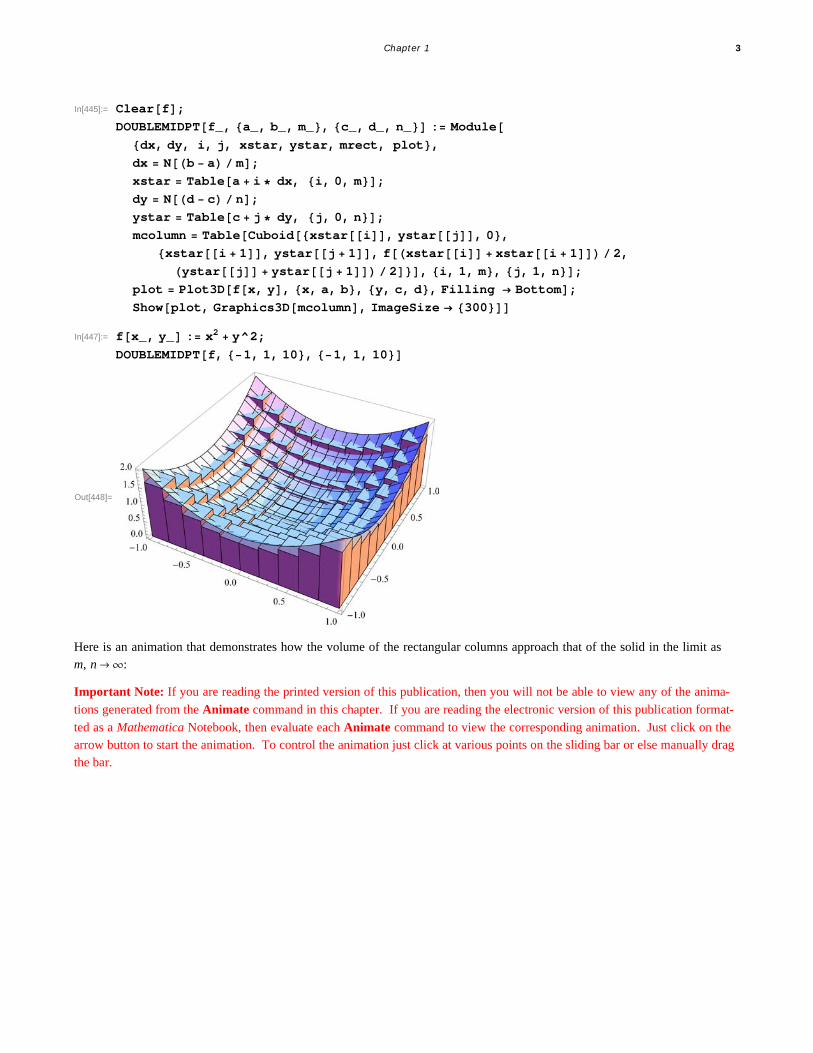
To see this limiting process visually, evaluate the following subroutine, called DOUBLEMIDPT, which plots the surface of thefunction corresponding to the double integral along with the rectangular columns defined by the double Riemann sum considered

in the previous subroutine MDOUBLERSUM.

2 Mathematica for Rogawski's Calculus

In[445]:= Clearf;

DOUBLEMIDPTf_, a_, b_, m_, c_, d_, n_ : Moduledx, dy, i, j, xstar, ystar, mrect, plot,dx Nb a m;xstar Tablea i dx, i, 0, m;dy Nd c n;ystar Tablec j dy, j, 0, n;

mcolumn TableCuboidxstari, ystarj, 0,xstari 1, ystarj 1, fxstari xstari 1 2,

ystarj ystarj 1 2, i, 1, m, j, 1, n;plot Plot3Dfx, y, x, a, b, y, c, d, Filling Bottom;

Showplot, Graphics3Dmcolumn, ImageSize 300In[447]:= fx_, y_ : x2 y^2;

DOUBLEMIDPTf, 1, 1, 10, 1, 1, 10

Out[448]=

Here is an animation that demonstrates how the volume of the rectangular columns approach that of the solid in the limit asm, nØ¶:

Important Note: If you are reading the printed version of this publication, then you will not be able to view any of the anima-

tions generated from the Animate command in this chapter. If you are reading the electronic version of this publication format-

ted as a Mathematica Notebook, then evaluate each Animate command to view the corresponding animation. Just click on thearrow button to start the animation. To control the animation just click at various points on the sliding bar or else manually dragthe bar.

Chapter 1 3

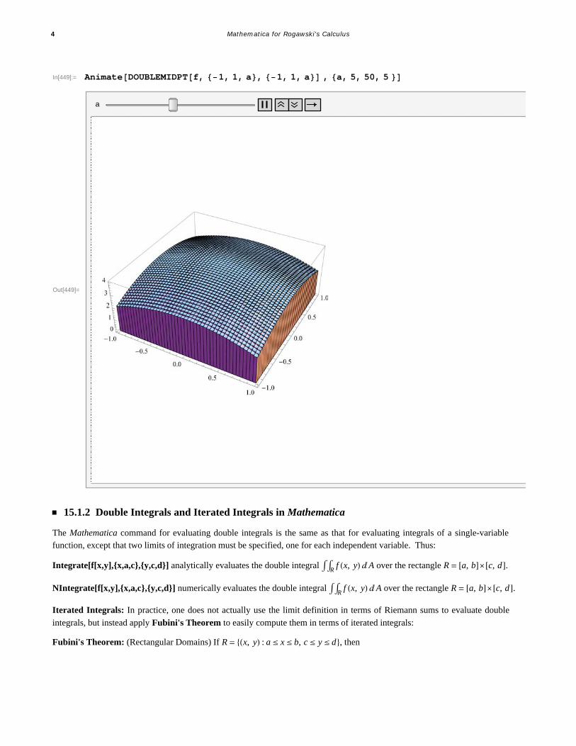
In[449]:= AnimateDOUBLEMIDPTf, 1, 1, a, 1, 1, a , a, 5, 50, 5

Out[449]=

a

ü 15.1.2 Double Integrals and Iterated Integrals in Mathematica

The Mathematica command for evaluating double integrals is the same as that for evaluating integrals of a single-variablefunction, except that two limits of integration must be specified, one for each independent variable. Thus:

Integrate[f[x,y],{x,a,c},{y,c,d}] analytically evaluates the double integral Rf x, y „A over the rectangle R = a, bä c, d.

NIntegrate[f[x,y],{x,a,c},{y,c,d}] numerically evaluates the double integral Rf x, y „A over the rectangle R = a, bä c, d.

Iterated Integrals: In practice, one does not actually use the limit definition in terms of Riemann sums to evaluate double

integrals, but instead apply Fubini's Theorem to easily compute them in terms of iterated integrals:

Fubini's Theorem: (Rectangular Domains) If R = x, y : a § x § b, c § y § d, then


R

f x, y „A = a

b

c

d

f x, y „ y „ x = c

d

a

b

f x, y „ x „ y

Thus, Mathematica will naturally apply Fubini's Theorem whenever possible to analytically determine the answer. Depending onthe form of the double integral, Mathematica may resort to more sophisticated integration techniques, such as contour integration,which are beyond the scope of this text.

Example 15.2. Calculate the volume of the solid bounded below by the surface f x = x2 + y2 and above the rectangleR = -1, 1ä -1, 1.Solution: The volume of the solid is given by the double integral R

f x, y „A. To evaluate it, we use the Integrate command:

In[450]:= fx_, y_ : x^2 y^2;

Integratefx, y, x, 1, 1, y, 1, 1

Out[451]=8

3

This confirms the conjecture that we made in the previous example for the exact volume.

NOTE: Observe that we obtain the same answer by explicitly computing this double integral as an integrated integral as follows.Moreover, for rectangular domains, the order of integration does not matter.

In[452]:= IntegrateIntegratefx, y, x, 1, 1, y, 1, 1IntegrateIntegratefx, y, y, 1, 1, x, 1, 1

Out[452]=8

3

Out[453]=8

3

Example 15.3. Compute the double integral Rx e-y2

„A on the rectangle R = 0, 1ä 0, 1.Solution: Observe that the Integrate command here gives us an answer in terms of the non-elementary error function Erf:

In[454]:= Integratex E^y^2, x, 0, 1, y, 0, 1

Out[454]=1

4 Erf1

This is because the function f x, y = x e-y2 has no elementary anti-derivative with respect to y due to the Gaussian factor e-y2

(bell curve). Thus, we instead use the NIntegrate Command to numerically approximate the double integral:

In[455]:= NIntegratex E^y^2, x, 0, 1, y, 0, 1Out[455]= 0.373412

ü Exercises

1. Consider the function f x, y = 16 - x2 - y2 defined over the rectangle R = 0, 2ä -1, 3.a. Use the subroutine MDOUBLERSUM to compute the double Riemann sum Sm,n of f x, y over R for m = 2 and n = 2.

b. Repeat part a) by generating a table of double Riemann sums for m = 10 k and n = 10 k where k = 1, 2, ..., 10. Make a

conjecture for the exact value of Rf x, y „A.

c. Find a formula for Sm,n in terms of m and n. Verify your conjecture in part b) by evaluating limm,nØ¶Sm,n.

Chapter 1 5

d. Directly compute Rf x, y „A using the Integrate command.

2. Repeat Exercise 1 but with f x, y = 1 + x 1 + y 1 + x y defined over the rectangle R = 0, 1ä 0, 1.

3. Evaluate the double integral x4 + y4 „A over the rectangle R = -2, 1ä -1, 2 using both the Integrate and

NIntegrate commands. How do the two answers compare?

4. Calculate the volume of the solid lying under the surface z = e-yx + y2 and over the rectangle R = 0, 2ä 0, 3. Then make a

plot of this solid.

5. Repeat Exercise 4 but with z = sinx2 + y2 and rectangle R = - p , p ä - p , p .6. Evaluate the double integral R

f x, y „A where f x, y = x y cosx2 + y2 and R = -p, pä -p, p. Does your answer

make sense? Make a plot of the solid corresponding to this double integral to intuitively explain your answer. HINT: Considersymmetry.

7. Find the volume of solid bounded between the two hyperbolic paraboloids (saddles) z = 1 + x2 - y2 and z = 3 - x2 + y2 overthe rectangle R = -1, 1ä -1, 1.8. Find the volume of the solid bounded by the planes z = 2 x, z = -3 x + 2, y = 0, y = 1, and z = 0.

ü 15.2 Double Integral over More General Regions


For domains of integration that are non-rectangular but still simple, that is, bounded between two curves, Fubini's Theoremcontinues to hold. There are two types to consider:

Fubini's Theorem: (Simple Domains)

Type I (Vertically Simple): If D = x, y : a § x § b, ax § y § bx, then

D

f x, y „A = a

b

ax

bxf x, y „ y „ x

The corresponding Mathematica command is Integrate[f[x,y],{x,a,b},{y,a[x],b[x]}].

Type II (Horizontally Simple): If D = x, y : c § y § d, ay § x § by, then

D

f x, y „A = c

d

ay

byf x, y „ x „ y

The corresponding Mathematica command is Integrate[f[x,y],{y,c,d},{x,a[y],b[y]}].

Warning: Be careful not to reverse the order of integration prescribed for either type. For example, evaluating the command

Integrate[f[x,y],{y,a[x],b[x]},{x,a,b}] for Type I (x and y are reversed) will lead to incorrect results.

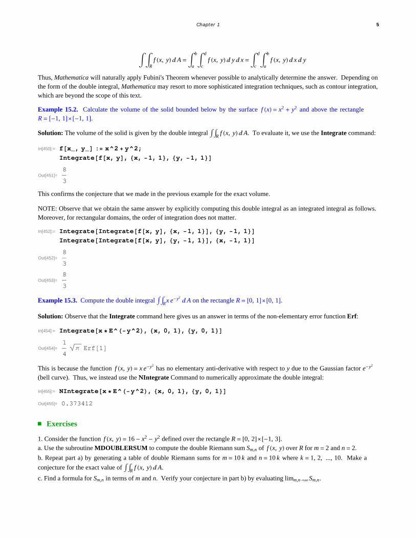
Example 15.4. Calculate the volume of the solid bounded below by the surface f x, y = 1 - x2 + y2 and above the domain Dbounded by x = 0, x = 1, y = x, and y = 1 + x2.

Solution: We observe that x = 0 and x = 1 represent the left and right boundaries, respectively, of D. Therefore, we plot thegraphs of the other two equations along the x-interval 0, 2 to visualize D (shaded in the following plot):


In[456]:= Clearx, yplot1 Plotx, 1 x^2, x, 0, 1, Filling 1 2, ImageSize 250

Out[457]=

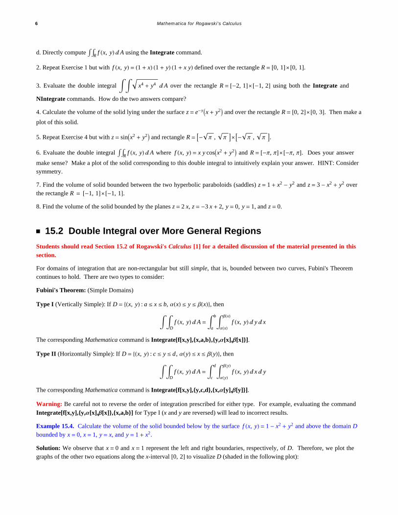
Here is a plot of the corresponding solid situated over D:

In[458]:= fx_, y_ 1 x^2 y^2;

plot3 Plot3Dfx, y, x, 0, 1, y, x, 1 x^2, Filling Bottom,ViewPoint 1, 1, 1, PlotRange 0, 4, ImageSize 250

Out[459]=

To compute the volume of this solid given by Df x, y „A, we describe D as a vertically simple domain where 0 § x § 1 and

x § y § 1 + x2 and apply Fubini's Theorem to evaluate the corresponding iterated integral 0

1x

1+x2

f x, y „ y „ x (remember to use

the correct order of integration):

In[460]:= Integratefx, y, x, 0, 1, y, x, 1 x2

Out[460]=29

21

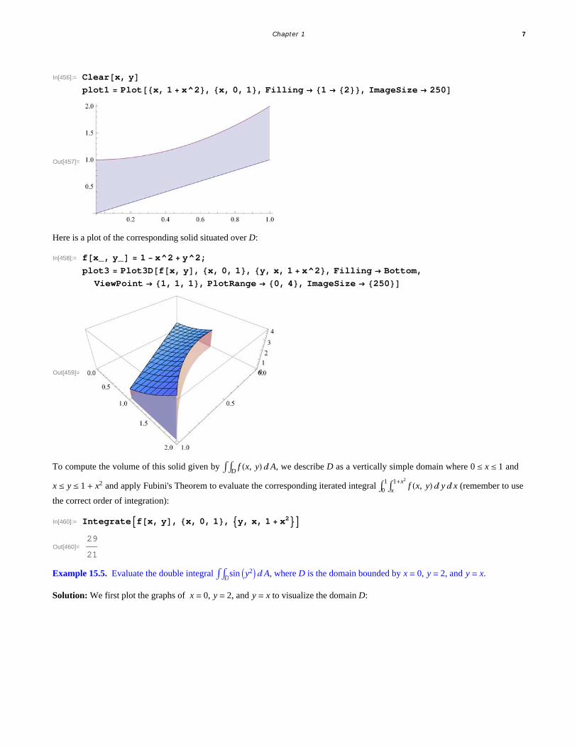
Example 15.5. Evaluate the double integral Dsin y2 „A, where D is the domain bounded by x = 0, y = 2, and y = x.

Solution: We first plot the graphs of x = 0, y = 2, and y = x to visualize the domain D:

Chapter 1 7

In[461]:= plot1 ContourPlotx 0, y 2, y x,

x, 0.5, 2.5, y, 0.5, 2.5, ImageSize 250

Out[461]=

-0.5 0.0 0.5 1.0 1.5 2.0 2.5

-0.5

0.0

0.5

1.0

1.5

2.0

2.5

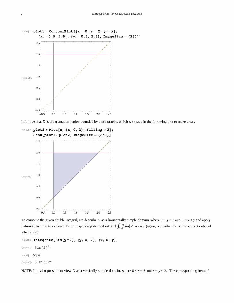
It follows that D is the triangular region bounded by these graphs, which we shade in the following plot to make clear:

In[462]:= plot2 Plotx, x, 0, 2, Filling 2;

Showplot1, plot2, ImageSize 250

Out[463]=

To compute the given double integral, we describe D as a horizontally simple domain, where 0 § y § 2 and 0 § x § y and apply

Fubini's Theorem to evaluate the corresponding iterated integral 0

20

ysiny2 „ x „ y (again, remember to use the correct order of

integration):

In[464]:= IntegrateSiny^2, y, 0, 2, x, 0, yOut[464]= Sin22

In[465]:= NOut[465]= 0.826822

NOTE: It is also possible to view D as a vertically simple domain, where 0 § x § 2 and x § y § 2. The corresponding iterated


integral 02x

2siny2 „ y „ x gives the same answer, as it should by Fubini's Theorem:

In[466]:= IntegrateSiny^2, x, 0, 2, y, x, 2Out[466]= Sin22

Observe that it is actually impossible to evaluate this iterated integral by hand since there is no elementary formula for the anti-derivative of siny2 with respect to y. Thus, if necessary, Mathematica automatically switches the order of integration by

converting from one type to the other.

ü Exercises

In Exercises 1 through 4, evaluate the given iterated integrals and plot the solid corresponding to each one.

1. 0

10

x24 - x2 + y2 „ y „ x 2. 0

40

2-y2

x2 y „ x „ y

3. 0p0

sin qr2 cosq „ r „q 4. 0

10x y

1+x y„ y „ x

In Exercises 5 through 8, evaluate the given double integrals and plot the solid corresponding to each one.

5. Dx + y „A, D = x, y : 0 § x § 3, 0 § y § x

6. Dx + y „A, D = x, y : 0 § x § 1 - y2, 0 § y § 1

7. Dex+y „A, where D = x, y : x2 + y2 § 4

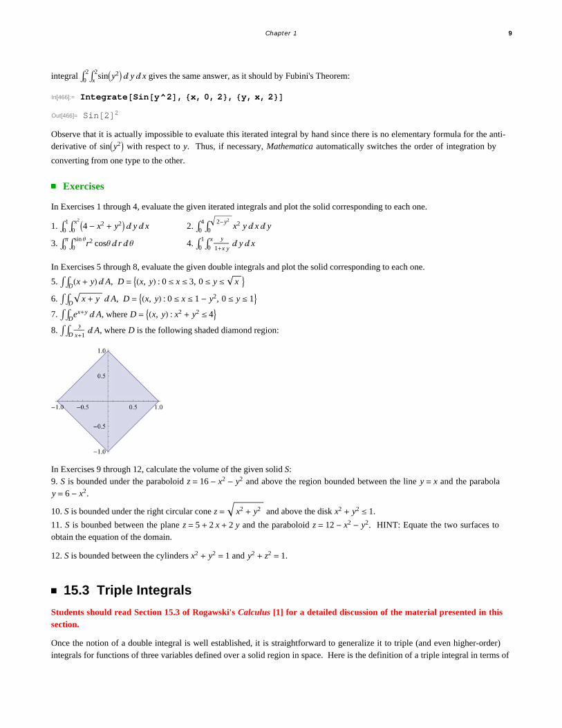
8. D

y

x+1„A, where D is the following shaded diamond region:

In Exercises 9 through 12, calculate the volume of the given solid S:9. S is bounded under the paraboloid z = 16 - x2 - y2 and above the region bounded between the line y = x and the parabolay = 6 - x2.

10. S is bounded under the right circular cone z = x2 + y2 and above the disk x2 + y2 § 1.

11. S is bounbed between the plane z = 5 + 2 x + 2 y and the paraboloid z = 12 - x2 - y2. HINT: Equate the two surfaces toobtain the equation of the domain.

12. S is bounded between the cylinders x2 + y2 = 1 and y2 + z2 = 1.

ü 15.3 Triple Integrals


Once the notion of a double integral is well established, it is straightforward to generalize it to triple (and even higher-order)integrals for functions of three variables defined over a solid region in space. Here is the definition of a triple integral in terms of

Chapter 1 9

triple Riemann sums for a function f x, y, z defined on a box region B = x, y, z : a § x § b, c § y § d, p § z § q (refer to yourcalculus text for details):

B

f x, y „V = limPØ¶

i=1

m

j=1

n

k=1

p

f xijk , yijkDVijk

where the notation is analogous to that used for double integrals in Section 15.1 of this text. Of course, Fubini's Theorem alsogeneralizes to triple integrals:

Fubini's Theorem: (Box Domains) If B = x, y, z : a § x § b, c § y § d, p § z § q, then

B

f x, y „V = a

b

c

d

p

q

f x, y „ z „ y „ x

The corresponding Mathematica commands are:

Integrate[f[x,y,z],{x,a,c},{y,c,d},{z,e,f}] analytically evaluates the triple integral Bf x, y „V over the box

B = a, bä c, dä e, f . NIntegrate[f[x,y],{x,a,c},{y,c,d},{z,e,f}] numerically evaluates the triple integral B

f x, y „V over the rectangle

B = a, bä c, dä e, f . NOTE: For box domains, the order of integration does not matter so that it is possible to write five other versions of triple iteratedintegrals besides the one given in Fubini's Theorem.

Example 15.6. Calculate the triple integral Bx y z „V over the box B = 0, 1ä 2, 3ä 4, 5.

Solution: We use the Integrate command to calculate the given triple integral.

In[467]:= Integratex y z, x, 0, 1, y, 2, 3, z, 4, 5

Out[467]=45

8

Volume as Triple Integral: Recall that if a solid region W is bounded between two surfaces yx, y and fx, y, where both aredefined on the same domain D with yx, y § fx, y, then its volume V can be expressed by the triple integral

V = W

1 „V = Dyx,y

fx,y1 „ z „A

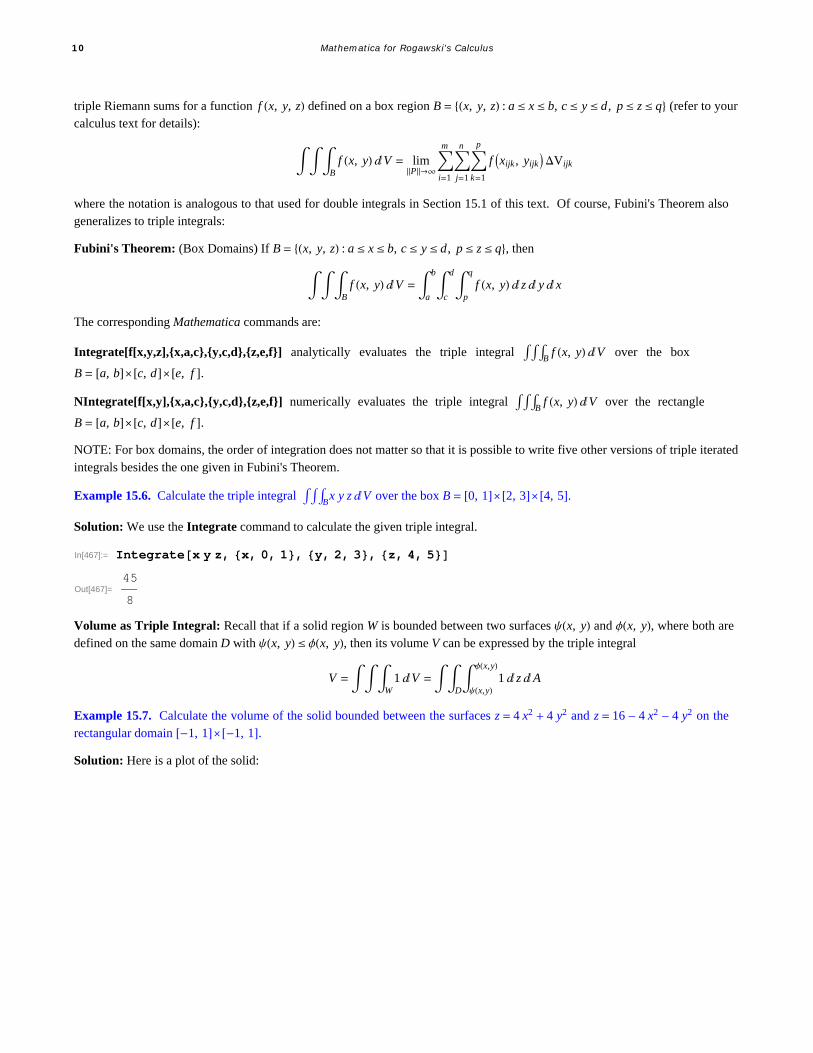
Example 15.7. Calculate the volume of the solid bounded between the surfaces z = 4 x2 + 4 y2 and z = 16 - 4 x2 - 4 y2 on therectangular domain -1, 1ä -1, 1.Solution: Here is a plot of the solid:


In[468]:= Plot3D4 x^2 4 y^2, 16 4 x^2 4 y^2, x, 1, 1, y, 1, 1,

Filling 1 8, 2 8, ImageSize 250, ImagePadding 15, 15, 15, 15

Out[468]=

The volume of the solid is given by the triple iterated integral -11 -1

1 4 x2+4 y2

16-4 x2-4 y2

1 „ z „ y „ x:

In[469]:= Integrate1, x, 0, 1, y, 1, 0, z, 4 x^2 4 y^2, 16 4 x^2 y^2

Out[469]=35

3

ü Exercises

In Exercises 1 through 4, evaluate the given iterated integrals:

1. 0

10

x0

y2x + y + z „ z „ y „ x 2. 0

30

sin y0

y +zx y z „ x „ z „ y

3. 0p0

q0r cos q

r z2 „ z „ r „q 4. 01 x

1 01-y

z log1 + x y „ z „ y „ x

In Exercises 5 through 8, evaluate the given triple integrals:

5. Wx + y z „V , where W = x, y, z : 0 § x § 1, 0 § y § x , 0 § z § y2.

6. Wsin y „V , where W lies under the plane z = 1 + x + y and above the triangular region bounded by x = 0, x = 2, and

y = 3 x.

7. Wz „V , where W is bounded by the paraboloid z = 4 - x2 - y2 and z = 0.

8. Wf x, y, z „V , where f x, y, z = z2 and W is bounded between the cone z = x2 + y2 and z = 9.

9. The triple integral 0

1x21-x20

2-x-2 y„ z „ y „ x represents the volume of a solid S. Evaluate this integral. Then make a plot of S

and describe it.

10. Midpoint Rule for Triple Integrals:

a. Develop a subroutine called MTRIPLERSUM to compute the triple Riemann sum of the triple integral Bf x, y, z „V

over the box domain B = x, y, z : a § x § b, c § y § d, p § z § q for uniform partitions and using the center midpoint of each

sub-box as base point. HINT: Modify the subroutine MDOUBLERSUM in Section 15.1 of this text.

b. Use your subroutine MTRIPLESUM in part a) to compute the triple Riemann sum of Bx2 + y2 + z232 „V over the box

B = x, y, z : 0 § x § 1, 0 § y § 2, 0 § z § 3 by dividing B into 48 equal sub-boxes, that is, cubes having side length of 1/2.

Chapter 1 11

c. Repeat part b) by dividing B into cubes having side length of 1/4 and more generally into cubes having side length of 1 2n forn sufficiently large in order to obtain an approximation accurate to 2 decimal places.

d. Verify your answer in part c) using Mathematica's NIntegrate command.

ü 15.4 Integration in Polar, Cylindrical, and Spherical Coordinates


ü 15.4.1 Double Integrals in Polar Coordinates

The following Change of Variables Formula converts a double integral in rectangular coordinates to one in polar coordinates:

Change of Variables Formula (Polar Coordinates):

I. Polar Rectangles: If R = r, q : q1 § q § q2, r1 § r § r2, then

R

f x, y „A = q1

q2

r1

r2

f r cos q, r sin q r „ r „q

II. Polar Regions: If D = r, q : q1 § q § q2, aq § r § bq, then

D

f x, y „A = q1

q2

aq

bqf r cos q, r sin q r „ r „q

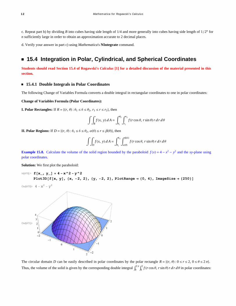
Example 15.8. Calculate the volume of the solid region bounded by the paraboloid f x = 4 - x2 - y2 and the xy-plane usingpolar coordinates.

Solution: We first plot the paraboloid:

In[470]:= fx_, y_ 4 x^2 y^2

Plot3Dfx, y, x, 2, 2, y, 2, 2, PlotRange 0, 4, ImageSize 250Out[470]= 4 x2 y2

Out[471]=

The circular domain D can be easily described in polar coordinates by the polar rectangle R = r, q : 0 § r § 2, 0 § q § 2 p.Thus, the volume of the solid is given by the corresponding double integral 0

2 p0

2f r cos q, r sin q r „ r „q in polar coordinates:


In[472]:= Clearr, ;

Integrater fr Cos, r Sin, r, 0, 2, , 0, 2 PiOut[473]= 8

Observe that here f x, y simplifies nicely in polar coordinates:

In[474]:= fr Cos, r SinSimplify

Out[474]= 4 r2 Cos2 r2 Sin2

Out[475]= 4 r2

NOTE: Evaluating the same double integral in rectangular coordinates by hand would be quite tedious. This is not a problemwith Mathematica, however:

In[476]:= Integratefx, y, x, 2, 2, y, Sqrt4 x^2, Sqrt4 x^2Out[476]= 8

ü 15.4.2 Triple Integrals in Cylindrical Coordinates

The following Change of Variables Formula converts a triple integral in rectangular coordinates to one in cylindrical coordinates:

Change of Variables Formula (Cylindrical Coordinates): If a solid region W is described by q1 § q § q2, aq § r § bq, andz1r, q § z § z2r, q, then

W

f x, y, z „V = q1

q2

aq

bq

z1r,q

z2r,qf r cos q, r sin q, z r „ z „ r „q

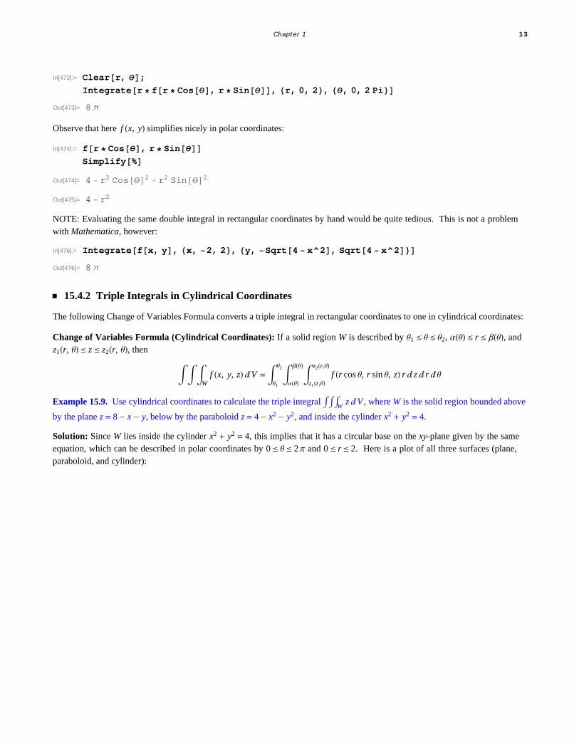
Example 15.9. Use cylindrical coordinates to calculate the triple integral Wz „V , where W is the solid region bounded above

by the plane z = 8 - x - y, below by the paraboloid z = 4 - x2 - y2, and inside the cylinder x2 + y2 = 4.

Solution: Since W lies inside the cylinder x2 + y2 = 4, this implies that it has a circular base on the xy-plane given by the sameequation, which can be described in polar coordinates by 0 § q § 2 p and 0 § r § 2. Here is a plot of all three surfaces (plane,paraboloid, and cylinder):

Chapter 1 13

In[477]:= plotplane Plot3D8 x y, x, 2, 2, y, 2, 2;

plotparaboloid Plot3D4 x^2 y^2, x, 2, 2, y, 2, 2;plotcylinder ParametricPlot3D2 Cos, 2 Sin, z, , 0, 2 , z, 0, 12;Showplotplane, plotparaboloid, plotcylinder, PlotRange All, ImageSize 250

Out[480]=

Since W is bounded in z by 4 - x2 - y2 § z § 8 - x - y, or in cylindrical coordinates, 4 - r cos q - r sin q § z § 4 - r2, it followsthat the given triple integral transforms to

02 p0

24-r2

4-r cos q-r sin qz r „ z „ r „q

Evaluating this integral in Mathematica yields the answer

In[481]:= Integratez r, , 0, 2 , r, 0, 2,z, 4 r Cos r Sin, 8 r Cos r Sin

Out[481]= 96

ü 15.4.3 Triple Integrals in Spherical Coordinates

The following Change of Variables Formula converts a triple integral in rectangular coordinates to one in spherical coordinates:

Change of Variables Formula (Spherical Coordinates): If a solid region W is described by q1 § q § q2, f1 § f § f2, andr1q, f § r § r2q, f, then

W

f x, y, z „V = q1

q2

f1

f2

r1q,f

r2q,ff r cos q sin f, r sin q sin f, r cos f r2 sinf „ r „f „q

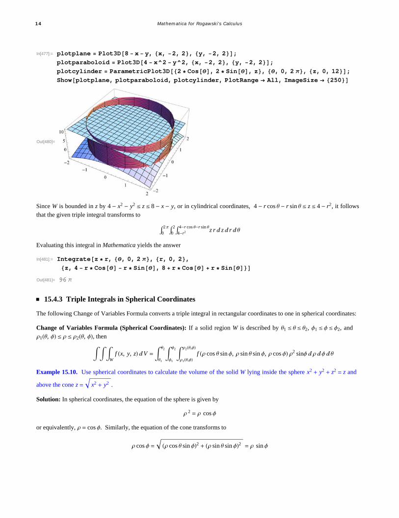
Example 15.10. Use spherical coordinates to calculate the volume of the solid W lying inside the sphere x2 + y2 + z2 = z and

above the cone z = x2 + y2 .

Solution: In spherical coordinates, the equation of the sphere is given by

r 2 = r cos f

or equivalently, r = cos f. Similarly, the equation of the cone transforms to

r cos f = r cos q sin f2 + r sin q sin f2 = r sin f


It follows that cos f = sin f, or f = p 4. Therefore, the cone makes an angle of 45 degrees with respect to the z-axis, as shown inthe following plot along with the top half of the sphere:

In[482]:= Clearplotcone ParametricPlot3D Cos SinPi 4, Sin SinPi 4, CosPi 4,

, 0, 2 Pi, , 0, Sqrt2 2;plotsphere ParametricPlot3DCos Cos Sin,

Cos Sin Sin, Cos Cos, , 0, 2 Pi, , 0, Pi 4;

Showplotcone, plotsphere, PlotRange All, ViewPoint 1, 1, 1 4,ImageSize 250

Out[485]=

It is now clear that the solid W is described by 0 § q § 2 p, 0 § f § p 4, and 0 § r § cos f. Thus, its volume is given by the tripleintegral

0

2 p

0

p4

0

cos f

r2 sin f „ r „f „q

which in Mathematica evaluates to

In[486]:= Integrate^2 Sin, , 0, 2 Pi, , 0, Pi 4, , 0, Cos

Out[486]=

8

ü Exercises

In Exercises 1 through 4, evaluate the given double integral by converting to polar coordinates:

1. -11

- 1-x2

1-x2 1 - x2 - y2 „ y „ x 2. 020

4-x2

e-x2+y2 „ y „ x

3. Dx log y „A, where D is the annulus (donut-shaped region) with inner radius 1 and outer radius 3.

4. Darctan

y

x„A, where D is the region inside the cardioid r = 1 + cos t.

5. Use polar coordinates to calculate the volume of the solid that lies below the paraboloid z = x2 + y2 and inside the cylinderx2 + y2 = 2 y.

Chapter 1 15

6. Evaluate the triple integral 0

20

4-x2 0

4-x2-y2 x2 + y2 „ z „ y „ x by converting to cylindrical coordinates.

7. Use cylindrical coordinates to calculate the triple integral Wx2 + y 2 „V , where W is the solid bounded between the two

paraboloids z = x2 + y2 and z = 8 - x2 - y2.

8. Evaluate the triple integral -2

2 - 4-x2

4-x2 x2+y2

4-x2-y2 x2 + y2 + z2 „ z „ y „ x by converting to spherical coordinates.

9. The solid defined by the spherical equation r = sin f is called the torus.a. Plot the torus.b. Calculate the volume of the torus.

10. Ice-Cream Cone: A solid W in the shape of an ice-cream cone is bounded below by the cylinder z = x2 + y2 and above by

the sphere x2 + y2 + z2 = 8. Plot W and determine its volume.

ü 15.5 Applications of Multiple Integrals


Mass as Double Integral: Consider a lamina (thin plate) D in R2 with continous mass density rx, y. Then the mass of D isgiven by the double integral

M = Drx, y „A

where the domain of integration is given by the region that describes the lamina D.

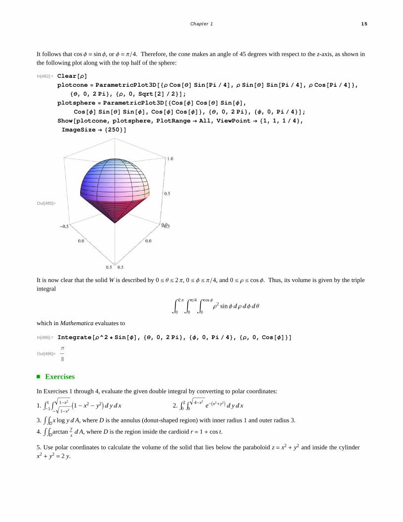
Example 15.11. Calculate the mass of the lamina D bounded between the parabola y = x2 and y = 4 with density rx, y = y.

Solution: Here is a plot of the lamina D (shaded):

In[487]:= Plotx^2, 4, x, 2, 2, ImageSize 250, Filling 2 1

Out[487]=

We can view D as a Type I region described by -2 § x § 2 and x2 § y § 4. Thus. the mass of the lamina is given by the doubleintegral:

In[488]:= Integratey, x, 2, 2, y, x^2, 4

Out[488]=128

5


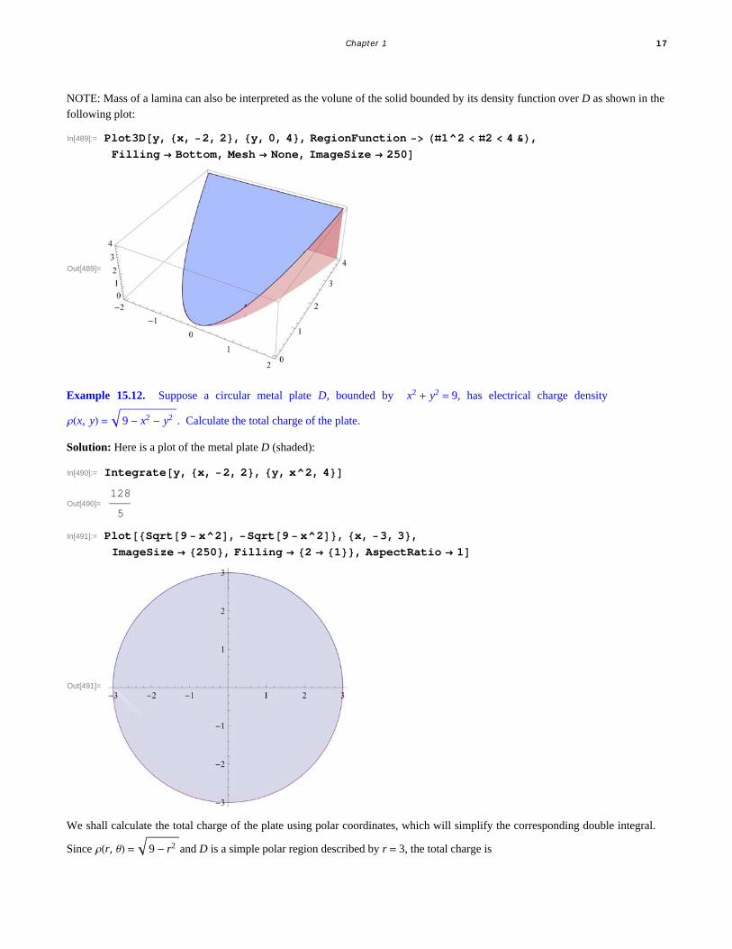
NOTE: Mass of a lamina can also be interpreted as the volune of the solid bounded by its density function over D as shown in thefollowing plot:

In[489]:= Plot3Dy, x, 2, 2, y, 0, 4, RegionFunction 1^2 2 4 &,

Filling Bottom, Mesh None, ImageSize 250

Out[489]=

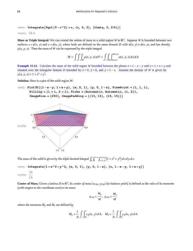
Example 15.12. Suppose a circular metal plate D, bounded by x2 + y2 = 9, has electrical charge density

rx, y = 9 - x2 - y2 . Calculate the total charge of the plate.

Solution: Here is a plot of the metal plate D (shaded):

In[490]:= Integratey, x, 2, 2, y, x^2, 4

Out[490]=128

5

In[491]:= PlotSqrt9 x^2, Sqrt9 x^2, x, 3, 3,

ImageSize 250, Filling 2 1, AspectRatio 1

Out[491]=

We shall calculate the total charge of the plate using polar coordinates, which will simplify the corresponding double integral.

Since rr, q = 9 - r2 and D is a simple polar region described by r = 3, the total charge is

Chapter 1 17

In[492]:= IntegrateSqrt9 r^2 r, r, 0, 3, theta, 0, 2 PiOut[492]= 18

Mass as Triple Integral: We can extend the notion of mass to a solid region W in R3. Suppose W is bounded between twosurfaces z = yx, y and z = fx, y, where both are defined on the same domain D with yx, y § fx, y, and has densityrx, y, z. Then the mass of W can be expressed by the triple integral

M = Wrx, y, z „V =

Dyx,y

fx,yrx, y, z „ z „A

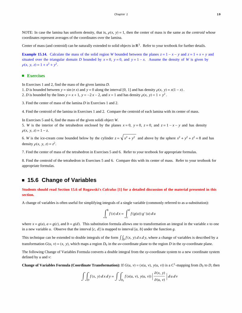
Example 15.13. Calculate the mass of the solid region W bounded between the planes z = 1 - x - y and z = 1 + x + y andsituated over the triangular domain D bounded by x = 0, y = 0, and y = 1 - x. Assume the density of W is given byrx, y, z = 1 + x2 + y2.

Solution: Here is a plot of the solid region W:

In[493]:= Plot3D1 x y, 1 x y, x, 0, 1, y, 0, 1 x, ViewPoint 1, 1, 1,

Filling 1 1, 2 1, Ticks Automatic, Automatic, 1, 2,ImageSize 250, ImagePadding 15, 15, 15, 15

Out[493]=

The mass of the solid is given by the triple iterated integral 010

1-x1-x-y1+x+y1 + x2 + y2 „ z „ y „ x:

In[494]:= Integrate1 x^2 y^2, x, 0, 1, y, 0, 1 x, z, 1 x y, 1 x y

Out[494]=14

15

Center of Mass: Given a lamina D in R2, its center of mass xCM, yCM (or balance point) is defined as the ratio of its moments(with respect to the coordinate axes) to its mass:

xCM =My

M, yCM =

Mx

M

where the moments My and Mx are defined by

My =1

A

Dx rx, y „A, Mx =

1

A

Dy rx, y „A


NOTE: In case the lamina has uniform density, that is, rx, y = 1, then the center of mass is the same as the centroid whosecoordinates represent averages of the coordinates over the lamina.

Center of mass (and centroid) can be naturally extended to solid objects in R3. Refer to your textbook for further details.

Example 15.14. Calculate the mass of the solid region W bounded between the planes z = 1 - x - y and z = 1 + x + y andsituated over the triangular domain D bounded by x = 0, y = 0, and y = 1 - x. Assume the density of W is given byrx, y, z = 1 + x2 + y2.

ü Exercises

In Exercises 1 and 2, find the mass of the given lamina D.1. D is bounded between y = sin p x and y = 0 along the interval 0, 1 and has density rx, y = x1 - x .2. D is bounded by the lines y = x + 1, y = -2 x - 2, and x = 1 and has density rx, y = 1 + y2 .

3. Find the center of mass of the lamina D in Exercises 1 and 2.

4. Find the centroid of the lamina in Exercises 1 and 2. Compare the centroid of each lamina with its center of mass.

In Exercises 5 and 6, find the mass of the given solidi object W.5. W is the interior of the tetrahedron enclosed by the planes x = 0, y = 0, z = 0, and z = 1 - x - y and has densityrx, y, z = 1 - z.

6. W is the ice-cream cone bounded below by the cylinder z = x2 + y2 and above by the sphere x2 + y2 + z2 = 8 and has

density rx, y, z = z2.

7. Find the center of mass of the tetrahedron in Exercises 5 and 6. Refer to your textbook for appropriate formulas.

8. Find the centroid of the tetrahedron in Exercises 5 and 6. Compare this with its center of mass. Refer to your textbook forappropriate formulas.

ü 15.6 Change of Variables


A change of variables is often useful for simplifying integrals of a single variable (commonly referred to as u-substitution):

a

b

f x „ x = c

d

f gu g ' u „u

where x = gu, a = gc, and b = gd. This substitution formula allows one to transformation an integral in the variable x to onein a new variable u. Observe that the interval c, d is mapped to interval a, b under the function g.

This technique can be extended to double integrals of the form Df x, y „ x „ y, where a change of variables is described by a

transformation Gu, v = x, y, which maps a region D0 in the uv-coordinate plane to the region D in the xy-coordinate plane.

The following Change of Variables Formula converts a double integral from the xy-coordinate system to a new coordinate systemdefined by u and v:

Change of Variables Formula (Coordinate Transformation): If Gu, v = xu, v, yu, v is a C1-mapping from D0 to D, then

D

f x, y „ x „ y = D0

f xu, v, yu, v ∑ x, y∑ u, v „u „v

Chapter 1 19

where ∑x,y∑u,v , referred to as the Jacobian of G and also denoted by Jac(G), is given by

JacG = ∑ x, y∑ u, v =

∑x

∑u

∑x

∑v∑y

∑u

∑y

∑v

=∑ x

∑u

∑ y

∑v-∑ x

∑v

∑ y

∑u

The Jacobian relates the area of any infinitesimal region inside D0 with the corresponding region inside D =GD0. In fact, if Gis a linear map, then Jac(G) is constant and is equal in magnitude to the ratio of the areas of D to that of D0:

Jacobian of a Linear Map: If Gu, v = A u + C v, B u + D v is a linear mapping from D0 to D, then Jac(G) is constant withvalue

JacG = A C

B D= A D - B C

Moreover,

AreaD = JacG AreaD0Refer to your textbook for a detailed discussion of transformations of plane regions.

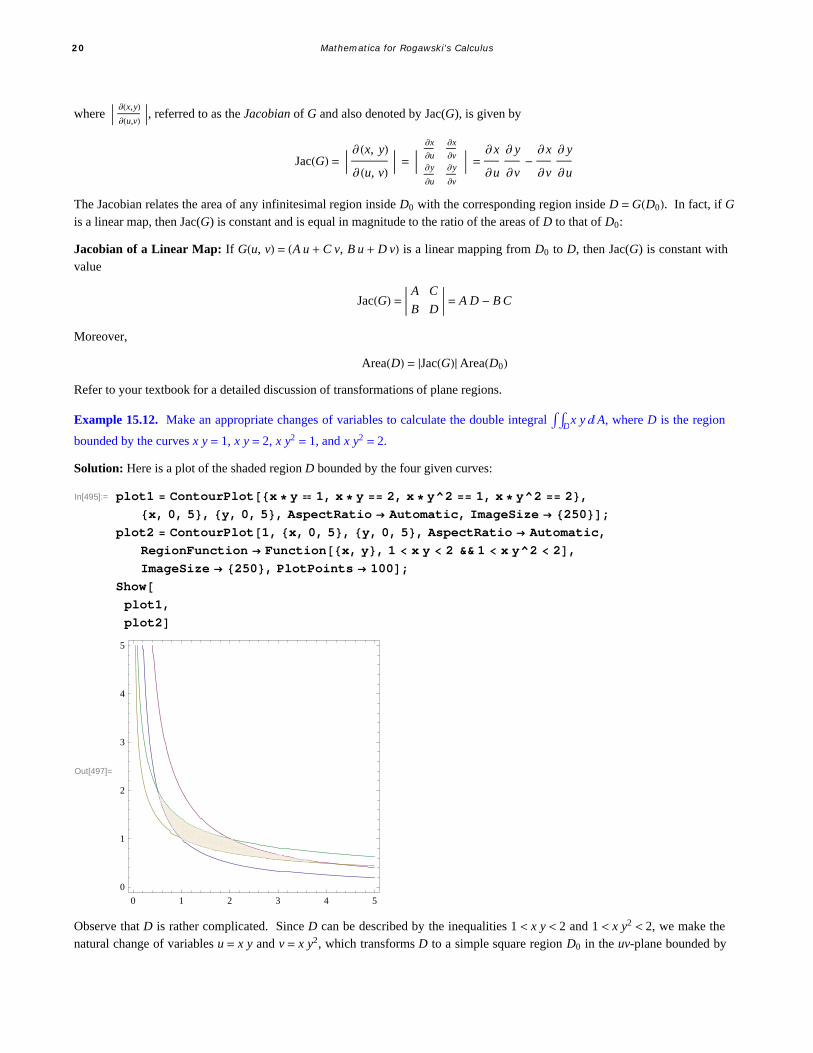
Example 15.12. Make an appropriate changes of variables to calculate the double integral Dx y „A, where D is the region

bounded by the curves x y = 1, x y = 2, x y2 = 1, and x y2 = 2.

Solution: Here is a plot of the shaded region D bounded by the four given curves:

In[495]:= plot1 ContourPlotx y 1, x y 2, x y^2 1, x y^2 2,x, 0, 5, y, 0, 5, AspectRatio Automatic, ImageSize 250;

plot2 ContourPlot1, x, 0, 5, y, 0, 5, AspectRatio Automatic,RegionFunction Functionx, y, 1 x y 2 && 1 x y^2 2,ImageSize 250, PlotPoints 100;

Showplot1,plot2

Out[497]=

0 1 2 3 4 5

0

1

2

3

4

5

Observe that D is rather complicated. Since D can be described by the inequalities 1 < x y < 2 and 1 < x y2 < 2, we make thenatural change of variables u = x y and v = x y2, which transforms D to a simple square region D0 in the uv-plane bounded by


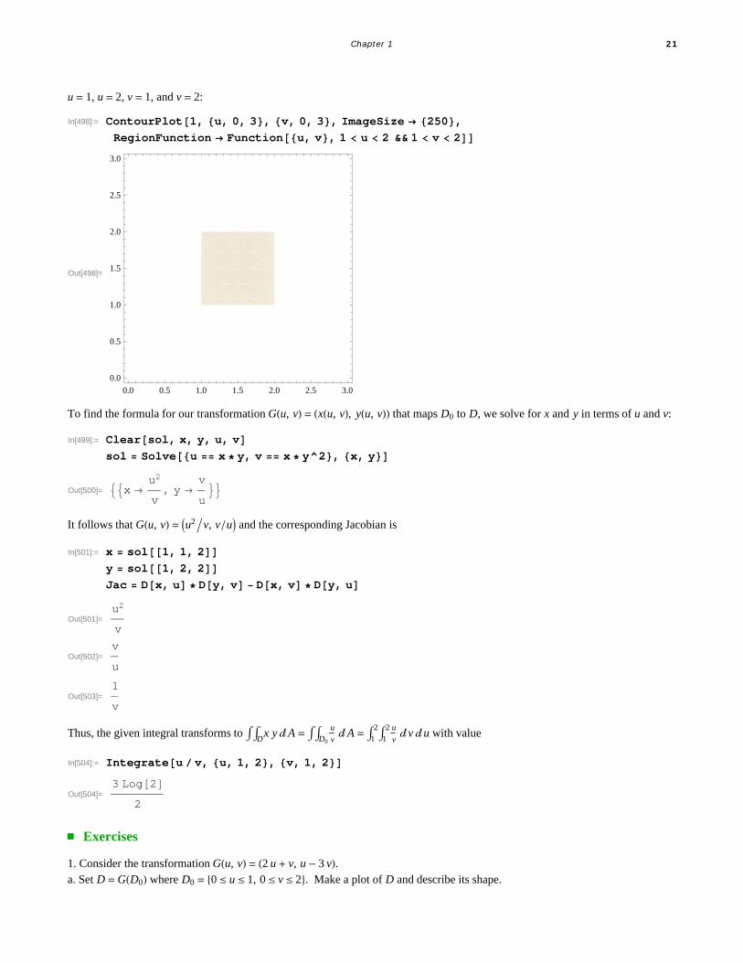
u = 1, u = 2, v = 1, and v = 2:

In[498]:= ContourPlot1, u, 0, 3, v, 0, 3, ImageSize 250,RegionFunction Functionu, v, 1 u 2 && 1 v 2

Out[498]=

0.0 0.5 1.0 1.5 2.0 2.5 3.0

0.0

0.5

1.0

1.5

2.0

2.5

3.0

To find the formula for our transformation Gu, v = xu, v, yu, v that maps D0 to D, we solve for x and y in terms of u and v:

In[499]:= Clearsol, x, y, u, vsol Solveu x y, v x y^2, x, y

Out[500]= x u2

v, y

v

u

It follows that Gu, v = u2 v, v u and the corresponding Jacobian is

In[501]:= x sol1, 1, 2y sol1, 2, 2Jac Dx, u Dy, v Dx, v Dy, u

Out[501]=u2

v

Out[502]=v

u

Out[503]=1

v

Thus, the given integral transforms to Dx y „A = D0

u

v„A = 1

21

2 u

v„v „u with value

In[504]:= Integrateu v, u, 1, 2, v, 1, 2

Out[504]=3 Log2

2

ü Exercises

1. Consider the transformation Gu, v = 2 u + v, u - 3 v.a. Set D =GD0 where D0 = 0 § u § 1, 0 § v § 2. Make a plot of D and describe its shape.

Chapter 1 21

b. Compute JacG.c. Compare the area of D with that of D0. How does this relate to JacG?

2. Compute the area of the ellipse x2

4+

y2

9= 1 by viewing it as a transformation of the unit circle u2 + v2 = 1 under a linear map

Gu, v = xu, v, yu, v and using the area relationship described by Jac(G).

3. Evaluate the integral Dx y „A, where D is the region in the first quadrant bounded by the equations y = x, y = 4 x, x y = 1,

and x y = 4. HINT: Consider the change of variables u = x y and v = y.

4. Evaluate the integral Dx + y x - y „A, where D is the parallelogram bounded by the lines x - y = 1, x - y = 3,

2 x + y = 0, and 2 x + y = 2. HINT: Consider the change of variables u = x - y and v = 2 x + y.

5. Evaluate the integral D

y

x„A, where D is the region bounded by the circles x2 + y2 = 1, x2 + y2 = 4 and lines y = x, y = 3 x.

HINT: Consider the change of variables u = x2 + y2 and v = y x.


Documents

Chapter 15 Multiple Integration - Rowan Universityusers.rowan.edu/~hassen/Mathematica/Volume III/Chapter 15.pdfChapter 15 Multiple Integration Useful Tip: If you are reading the electronic