Integration of Deformable Contours and a

Multiple Hypotheses Fisher Color Model for

Robust Tracking in Varying Illuminant

Environments

Francesc Moreno-Noguer a,∗, Alberto Sanfeliu a,Dimitris Samaras b

aInstitut de Robotica i Informatica IndustrialUPC-CSIC, Llorens i Artigas 4-6

08028, Barcelona, SpainbComputer Science Department

State University of New York at Stony BrookNY 11794-4400, USA

Abstract

In this paper we propose a new technique to perform figure-ground segmentationin image sequences of moving objects under varying illumination conditions. Unlikemost of the algorithms that adapt color, there is not the assumption of smoothchange of the viewing conditions. To cope with this, we propose the use of a newcolorspace that maximizes the foreground/background class separability based onthe ‘Linear Discriminant Analysis’ method. Moreover, we introduce a technique thatformulates multiple hypotheses about the next state of the color distribution (someof these hypotheses take into account small and gradual changes in the color modeland others consider more abrupt and unexpected variations) and the hypothesisthat generates the best object segmentation is used to remove noisy edges from theimage. This simplifies considerably the final step of fitting a deformable contourto the object boundary, thus allowing a standard snake formulation to successfullytrack nonrigid contours. In the same manner, the contour estimate is used to correctthe color model. The integration of color and shape is done in a stage called ‘sam-ple concentration’, introduced as a final step to the well-known CONDENSATIONalgorithm.

Key words: tracking, deformable contours, color adaption, particle filters.

Preprint submitted to Elsevier Science 3 February 2006

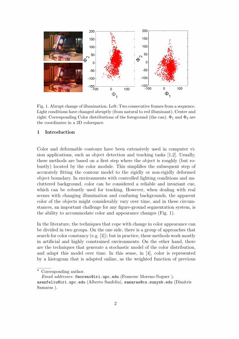
Fig. 1. Abrupt change of illumination. Left: Two consecutive frames from a sequence.Light conditions have changed abruptly (from natural to red illuminant). Center andright: Corresponding Color distributions of the foreground (the can). Φ1 and Φ2 arethe coordinates in a 2D colorspace.

1 Introduction

Color and deformable contours have been extensively used in computer vi-sion applications, such as object detection and tracking tasks [1,2]. Usually,these methods are based on a first step where the object is roughly (but ro-bustly) located by the color module. This simplifies the subsequent step ofaccurately fitting the contour model to the rigidly or non-rigidly deformedobject boundary. In environments with controlled lighting conditions and un-cluttered background, color can be considered a reliable and invariant cue,which can be robustly used for tracking. However, when dealing with realscenes with changing illumination and confusing backgrounds, the apparentcolor of the objects might considerably vary over time, and in these circum-stances, an important challenge for any figure-ground segmentation system, isthe ability to accommodate color and appearance changes (Fig. 1).

In the literature, the techniques that cope with change in color appearance canbe divided in two groups. On the one side, there is a group of approaches thatsearch for color constancy (e.g. [3]); but in practice, these methods work mostlyin artificial and highly constrained environments. On the other hand, thereare the techniques that generate a stochastic model of the color distribution,and adapt this model over time. In this sense, in [4], color is representedby a histogram that is adapted online, as the weighted function of previous

∗ Corresponding author.Email addresses: fmoreno@iri.upc.edu (Francesc Moreno-Noguer ),

asanfeliu@iri.upc.edu (Alberto Sanfeliu), samaras@cs.sunysb.edu (DimitrisSamaras ).

2

histograms and a predicted histogram. Yang and Lu [5], parameterize objectcolor by a unique gaussian, the mean and covariance of which are estimatedusing a linear combination of the parameters in previous gaussians. Raja andMcKenna [6] approximate color with a mixture of gaussians, and dynamicallyupdate it using a weighted sum of previous estimates with estimates based onnew data.

The drawback in all these approaches is that they assume that color variesslowly and that it can be predicted by a dynamic model based in only onehypothesis. However, this assumption does not suffice to cope with generalscenes, where the dynamics of the color distribution might follow an unknownor unpredictable path.

The main contributions of this paper are summarized below. They are thebuilding blocks of a system which does not impose constraints on the illumi-nant color of the scene:

• Fisher colorspace: Instead of using the classical RGB, rgb, XY Z or HSVcolorspaces, we propose the use of a colorspace efficient for the discrimina-tion between foreground and background classes. This colorspace will be the2D projection of the R, G and B components on the plane obtained from anonparametric Linear Discriminant Analysis (LDA) [7].

• Multihypotheses framework: The use of a particle filter formulation topredict the color distribution in subsequent iterations, offers robustness toabrupt and unexpected changes in the color appearance of the object. Inprevious work [8] we have suggested a similar multihypotheses frameworkto track objects in which color could be approximated by a unimodal dis-tribution, represented by a histogram. In the present work, we deal withmulticolored objects, approximated by a mixture of gaussians (MoG). Notethe difference between our work and all previous tracking approaches usinga particle filter formulation (e.g. [2,9,10]). While in these approaches themultihypotheses are formulated about the object position, in our methodwe formulate the multihypotheses about the color distribution of the object.

• Integration of color and deformable contours in a particle filterframework: The color estimation is used to generate a rough estimationabout the object position and remove noisy edges from the image. Thissimplifies the stage of fitting a deformable contour to the object boundary,and even with a standard snake formulation [11], nonrigid objects can beaccurately tracked in cluttered backgrounds with abrupt changes of illumi-nation. The fusion of the multihypotheses color model and the deformablecontour is done in a final stage that we have introduced to the well-knownCONDENSATION algorithm [2].

The basic steps of the algorithm are depicted in the flow diagram of Fig. 2, andin the following sections, a detailed description of each one of the modules will

3

Fig. 2. Flow diagram of the proposed algorithm. It is the input RGB image at timet. IFISHER

t represents the input image in the Fisher colorspace. St and St are theset of color distributions of the foreground and background, before and after the‘concentration’ stage, respectively. Ct is the resulting contour at time t.

be given. Fisher colorspace is described in Section 2. In Section 3 the objectcolor model and initialization step are presented. The dynamic model for gen-erating multiple hypotheses of the (object and background) color distributionsis depicted in Section 4. Section 5 deals with the global and local deformablemodel fitting process. In Section 6, the complete tracking algorithm and modeladaptation is explained in detail, and results and conclusions are presented inSections 7 and 8, respectively.

4

2 Fisher Colorspace

The selection of the colorspace is an important initial issue for any color-based figure-ground segmentation system. The typical selection criterion isbased on the invariance of the color representation to illumination changes,and according to this idea, color is usually represented by two componentsof the rgb, HSV or xyz 1 colorspaces. However, these representations are notrobust enough to cope with abrupt illumination changes. In this paper wepropose a different criterion and select a 2D colorspace that maximizes theseparability of the object and background classes.

Let x be a 3D vector with the color value of image pixels in RGB space, whichmust be classified as foreground (O) or background (B). When we are dealingwith multicolored objects, the parameterization of color distributions in 3Dcolorspace becomes very complex. To simplify, we reduce the dimensionalityto 2D by projecting the data on a plane Φ = [φ1, φ2] ∈ M3×2, that is, y = Φx,where y are the linearly transformed 2D coordinates used for classification.The most popular way to find the best linear features is the parametric versionof the Linear Discriminant Analysis method [12], where training data is usedto construct the within-class Sw and between-class Sb scatter matrices, in theNc-class problem defined as,

Sw =Nc∑i=1

P (Ci) E[(x|Ci − µi) (x|Ci − µi)

T]

=Nc∑i=1

P (Ci) Si

Sb =Nc∑i=1

P (Ci) E[(x − µo) (x − µo)

T] (1)

where P (Ci) is the prior of the ith class, µi and Si are its expected value vectorand covariance matrix, µo is the overall mean and x|Ci

indicates that samplex belongs to Ci class.

A typical criterion for class separability is formulated by the maximization

of J = trace((

ΦT SwΦ)−1 (

ΦT SbΦ))

, and searches for the separation of the

class means in the transformed Y -space (high Sb), while at the same timethe classes remain compact (small Sw). The classic LDA method maximizes Jby constructing the columns of Φ with the eigenvectors of S−1

w Sb having thehighest eigenvalues.

One of the limitations associated with this approach is that it produces atmost Nc − 1 feature projections, i.e, since Sb is computed from only Nc classmeans, S−1

w Sb will have at most Nc−1 non-zero eigenvalues, and the maximum

1 When the colorspace is represented by lowercase letters, the sum of the 3 colorcomponents has been normalized to one.

5

(a) (b) (c)

(d) (e)

(f) (g)

Fig. 3. Fisher Colorspace. (a) Training image. (b) Foreground. (c) Background. (d)Representation of image points in the RGB colorspace. (e) Hand-made classificationof image points in foreground (O) and background (B) classes. (f) Normalization ofcolorpoints, equivalent to a projection on the plane R + G + B = 1. The projectedclasses are not properly separated. (g) The projection of colorpoints on the Fisherplane gives a better discrimination between the O and B classes.

dimension of the projected Y -space will be Nc − 1. This can be solved by thenonparametric LDA [7], that computes Sb using local information and thek Nearest Neighbors (KNN) rule. In the 2-class problem discussed here, this

6

matrix (denoted Σb) is defined as,

Σb =1N

Nf∑i=1

wi

(xi|O − Mk

b (xi|O)) (

xi|O − Mkb (xi|O)

)T

+1N

Nb∑i=1

wi

(xi|B − Mk

f (xi|B)) (

xi|B − Mkf (xi|B)

)T

(2)

where Nf and Nb are the number of samples of O and B, N = Nf + Nb,Mk

j (xi) is the mean of the k nearest neighbors in class Cj to a point xi, andwi is a weighting function for deemphasizing samples far from the classificationboundary (see [7]).

Given two setsx1|O, · · · ,xNf |O

,x1|B, · · · ,xNb|B

of RGB pixel values used

as training data, the optimum linear mapping is obtained with the followingsteps:

• Calculate Sw with Eq. 1 and whiten the data with respect to it. That is,transform x to z = Λ−1/2ΩTx, where Λ and Ω are the eigenvalue and eigen-vector matrices of Sw.

• Select k and (in the Z-space) compute Σb using Eq. 2.• Select the two eigenvectors Ψ1, Ψ2 of Σb with the two largest eigenvalues.• The optimum linear mapping from the original RGB space to the discrim-

inant subspace (we call it Fisher colorspace) is given by y = ΨT Λ−1/2ΩTx.

In Fig. 3 we show the concept of Fisher colorspace. In the Results Sectionit will be shown that we obtain better rates of class classification using theFisher colorspace than using other 2D colorspaces.

For the rest of the paper we will represent the pixel values in the Fishercolorspace with the 2D vector y.

3 Color Model

After having selected the colorspace, the next step is to choose a modelfor representing the color distribution of the object and background. For amonochrome object, color histograms have been demonstrated to be an ef-fective technique (e.g.[8]). However, when the object to be modelled containsregions with different colors, the number of pixels representing each color canbe relatively low and a histogram representation may not suffice. In this case,a better approach is to use the MoG model, that expresses the conditionalprobability for a pixel y belonging to a multi-colored object O as a sum of Mo

gaussian components: p (y|O) =∑Mo

j=1p (y|j) P (j). Similarly, the backgroundcolor will be represented by a mixture of Mb gaussians.

7

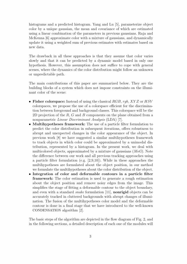
Fig. 4. Gaussian mixture components of O (the can) and B. Left image: Solid dotsand lines are O data points (in Fisher colorspace) and the variances of the gaussiancomponents, respectively. Hollow dots and dashed lines are B data and gaussians.Lower right image: p (O|y), where brighter points correspond to more likely pixels.

Given the foreground (O) and background (B) classes, the a posteriori prob-ability that a pixel y belongs to object O is computed using the Bayes rule:

p (O|y) =p (y|O) P (O)

p (y|O) P (O) + p (y|B) P (B)(3)

where P (O), P (B) represent the a priori probabilities of O and B, respec-tively. These prior values are approximated to the expected area ratios of theforeground and background classes in the image (see Fig. 4).

As in the problem of selecting the number of bins in histogram models, usingMoG conceals the challenge of choosing the number of gaussian componentsthat better adjust the data. We initialize this, with the modified EM algo-rithm proposed in [13], that is based on a Minimum Message Length criterionand iteratively fits and annihilates an initially large number of components(introduced by the user).

The initial configurations of the MoG for O and B, after learning, are param-eterized by:

Gε = [pε, µε, λε, θε] (4)

where ε = O,B, pε contains the priors for each gaussian component, µε

the centroids, λε the eigenvalues of the principal directions and θε the anglesbetween the principal directions with the horizontal. G = GO,GB will be thestate vector representing the color model.

8

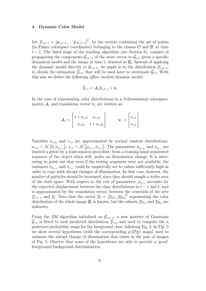
4 Dynamic Color Model

Let Yε,t−1 = [y1,t−1, . . .yNε,t−1]T , be the vectors containing the set of points

(in Fisher colorspace coordinates) belonging to the classes O and B, at timet − 1. The third stage of the tracking algorithm (see Section 6), consists ofpropagating the components Gε,t−1 of the state vector to Gε,t, given a specificdynamical model and the image at time t, denoted as Zt. Instead of applyingthe dynamic model directly to Gε,t−1, we apply it to the distribution Yε,t−1,to obtain the estimation Yε,t, that will be used later to reestimate Gε,t. Withthis aim we define the following affine random dynamic model:

Yε,t = AεYε,t−1 + vε

In the case of representing color distributions in a 2-dimensional colorspace,matrix Aε and translation vector vε are written as:

Aε =

⎡⎢⎣ 1 + aε,11 aε,12

aε,21 1 + aε,22

⎤⎥⎦ vε =

⎡⎢⎣ vε,1

vε,2

⎤⎥⎦

Variables aε,ij and vε,i are approximated by normal random distributions,

aε,ij ∼ N(0, σaε,ij

), vε,i ∼ N

(µvε,i

, σvε,i

). The parameters σaε,ij

and σvε,iare

learned a priori by a least-squares procedure, from a training hand segmentedsequence of the object when still, under an illumination change. It is inter-esting to point out that even if the testing sequences were not available, thevariances σaε,ij

and σvε,icould be empirically set to values sufficiently high in

order to cope with abrupt changes of illumination. In that case, however, thenumber of particles should be increased, since they should sample a wider areaof the state space. With respect to the rest of parameters, µvε,i

accounts forthe expected displacement between the class distributions in t − 1 and t, andis approximated by the translation vector between the centroids of the setsYε,t−1 and Yt. Note that the vector Yt = [YO,t,YB,t]

T representing the colordistribution of the whole image Zt is known, but the subsets YO,t and YB,t areunknown.

Using the EM algorithm initialized on Gε,t−1, a new mixture of GaussiansGε,t is fitted to each predicted distribution Yε,t, and used to compute the aposteriori probability maps for the foreground class, following Eq. 3. In Fig. 5we show several hypotheses (with the corresponding p (O|y) maps) used toestimate the abrupt change of illumination that exists in the pair of imagesof Fig. 5. Observe that some of the hypotheses are able to provide a ‘good’foreground/background discrimination.

9

Fig. 5. Several hypotheses and their respective p (O|y) map, corresponding to theabrupt illumination transition presented in Fig. 1.

5 Global and Local Deformable Model Fitting

As color segmentation usually only gives a rough estimation about the objectlocation, we use a deformable model [10,14] to fit its boundary and obtainmore precise information about its position. This process is highly simplifiedby using the data that is estimated by the color model (Section 4) in order

10

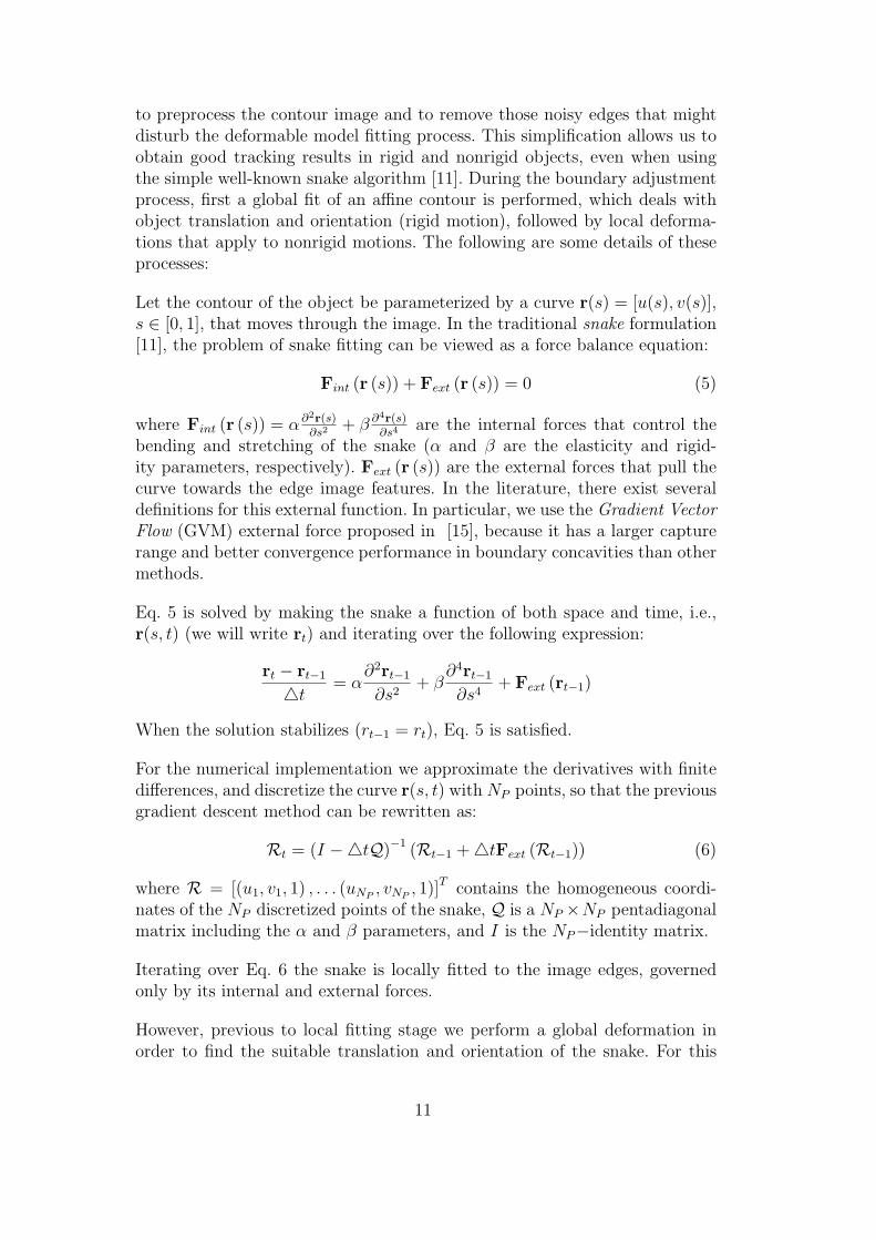
to preprocess the contour image and to remove those noisy edges that mightdisturb the deformable model fitting process. This simplification allows us toobtain good tracking results in rigid and nonrigid objects, even when usingthe simple well-known snake algorithm [11]. During the boundary adjustmentprocess, first a global fit of an affine contour is performed, which deals withobject translation and orientation (rigid motion), followed by local deforma-tions that apply to nonrigid motions. The following are some details of theseprocesses:

Let the contour of the object be parameterized by a curve r(s) = [u(s), v(s)],s ∈ [0, 1], that moves through the image. In the traditional snake formulation[11], the problem of snake fitting can be viewed as a force balance equation:

Fint (r (s)) + Fext (r (s)) = 0 (5)

where Fint (r (s)) = α∂2r(s)∂s2 + β ∂4r(s)

∂s4 are the internal forces that control thebending and stretching of the snake (α and β are the elasticity and rigid-ity parameters, respectively). Fext (r (s)) are the external forces that pull thecurve towards the edge image features. In the literature, there exist severaldefinitions for this external function. In particular, we use the Gradient VectorFlow (GVM) external force proposed in [15], because it has a larger capturerange and better convergence performance in boundary concavities than othermethods.

Eq. 5 is solved by making the snake a function of both space and time, i.e.,r(s, t) (we will write rt) and iterating over the following expression:

rt − rt−1

t= α

∂2rt−1

∂s2+ β

∂4rt−1

∂s4+ Fext (rt−1)

When the solution stabilizes (rt−1 = rt), Eq. 5 is satisfied.

For the numerical implementation we approximate the derivatives with finitedifferences, and discretize the curve r(s, t) with NP points, so that the previousgradient descent method can be rewritten as:

Rt = (I −tQ)−1 (Rt−1 + tFext (Rt−1)) (6)

where R = [(u1, v1, 1) , . . . (uNP, vNP

, 1)]T contains the homogeneous coordi-nates of the NP discretized points of the snake, Q is a NP ×NP pentadiagonalmatrix including the α and β parameters, and I is the NP−identity matrix.

Iterating over Eq. 6 the snake is locally fitted to the image edges, governedonly by its internal and external forces.

However, previous to local fitting stage we perform a global deformation inorder to find the suitable translation and orientation of the snake. For this

11

fitting, the following additional constraint of affine deformation is introducedto Eq. 6:

Rt = Rt−1HA = Rt−1

⎡⎢⎢⎢⎢⎢⎣

a11 a12 v1

a21 a22 v2

0 0 1

⎤⎥⎥⎥⎥⎥⎦

(7)

Combining Equations 6 and 7, we obtain the following iterative procedure forthe affine snake deformation:

(1) HA =(J TJ

)−1 J T (Rt−1 + Fext (Rt−1))where J = Rt−1 −tSRt−1

(2) Normalize HA using the component HA (3, 3)Set HA (3, 1) = HA (3, 2) = 0

(3) Rt = Rt−1HA

Steps 1−3 are iterated until the convergence of Rt and Rt−1. In Fig.6 we showthe results of the global and local fitting in a nonrigid movement.

6 Tracking Algorithm

In this Section, we will use the tools described previously to explain in detailthe whole method for tracking rigid and nonrigid objects in a cluttered envi-ronment and under changing illumination. The basic steps of the tracking al-gorithm follow the particle filter procedure, but we introduce a modification tothe classic CONDENSATION algorithm (analogous to the ICONDENSATIONtechnique [2]), and in order to ‘direct’ the search for the next iteration we adda final stage that concentrates the future hypotheses on those areas of thestate-space containing more information about p (O|y) (see Fig. 7). Moreover,in this final stage we fuse object color and shape information to obtain preciseresults about object pose. Next, we present the steps of our algorithm:

(1) Probability Density Function of the color point set: At time t,

a set of N samples S(n)t−1 (n = 1, . . . , N) with the same structure as G

(Eq. 4), is available from previous iteration. This set, parameterizes N

color distributions. Each sample has an associated weight π(n)t−1 and a

classification Y (n)t−1 = [Y(n)

O,t−1,Y(n)B,t−1]

T of the image colorpoints in the fore-ground and background sets. The whole set represents an approximationto p (Gt−1|Zt−1) where Zt−1 = Z0, . . . ,Zt−1 is the history of the images.

The algorithm aims to construct a new sample set S(n)t , π

(n)t to estimate

p (Gt|Zt) .(2) Sampling from p (Gt−1|Zt−1): A sampling with replacement is per-

formed N times on the set S(n)t−1, where each element has probability

12

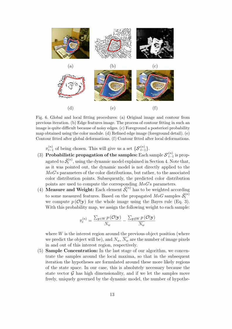
(a) (b) (c)

(d) (e) (f)

Fig. 6. Global and local fitting procedures: (a) Original image and contour fromprevious iteration. (b) Edge features image. The process of contour fitting in such animage is quite difficult because of noisy edges. (c) Foreground a posteriori probabilitymap obtained using the color module. (d) Refined edge image (foreground detail). (e)Contour fitted after global deformations. (f) Contour fitted after local deformations.

π(n)t−1 of being chosen. This will give us a set S ′(n)

t−1.(3) Probabilistic propagation of the samples: Each sample S ′(n)

t−1 is prop-

agated to S(n)t , using the dynamic model explained in Section 4. Note that,

as it was pointed out, the dynamic model is not directly applied to theMoG’s parameters of the color distributions, but rather, to the associatedcolor distribution points. Subsequently, the predicted color distributionpoints are used to compute the corresponding MoG’s parameters.

(4) Measure and Weight: Each element S(n)t has to be weighted according

to some measured features. Based on the propagated MoG samples S(n)t

we compute p (O|y) for the whole image using the Bayes rule (Eq. 3).With this probability map, we assign the following weight to each sample:

π(n)t =

∑y∈W p (O|y)

Nw

−∑

y/∈W p (O|y)

Nw

where W is the interest region around the previous object position (wherewe predict the object will be), and Nw, Nw are the number of image pixelsin and out of this interest region, respectively.

(5) Sample Concentration: In the last stage of our algorithm, we concen-trate the samples around the local maxima, so that in the subsequentiteration the hypotheses are formulated around these more likely regionsof the state space. In our case, this is absolutely necessary because thestate vector G has high dimensionality, and if we let the samples movefreely, uniquely governed by the dynamic model, the number of hypothe-

13

Fig. 7. Left: Steps of the classic CONDENSATION algorithm (Figure adaptedfrom [10]). Right: In our implementation we have included a final stage called ‘sam-ple concetration’.

ses needed to find the samples representing a correct color configuration,is extremely high.

The concentration is performed by taking the sample with maximumweight, π∗

t = maxπ(1)t , · · · , π

(n)t and based on the a posteriori map gen-

erated by this sample, the object of interest is accurately segmented fromthe image using the deformable model fitting procedure explained in Sec-tion 5. The various substeps of this stage, can be summarized as follows:(a) Using morphologic operations on the probability map image, a coarse

approximation of object shape is obtained that allows us to eliminatenoisy edges from the original image (Fig. 6b,c,d).

(b) The contour of the object in the previous iteration, is used as ini-tialization of an affine snake, that is adjusted (only by affine defor-mations) to the image of refined edges (Fig. 6e) in order to solve theglobal deformation. Next, to cope with nonrigid deformations theprocess is repeated with a non-affine snake (Fig. 6f).

(c) Once the boundary of the object has been accurately detected, thecolor estimates are refined. Inner image pixels are separated from

outer pixels and the vector Y∗t =

[Y∗

O,t,Y∗B,t

]Tis generated. Mixtures

of gaussians are fitted to these color distributions (using the EM

algorithm), giving a state vector S∗t , around which samples S(n)

t are ‘concentrated’ with the equation S

(n)t = (1− a)S

(n)t + aS∗

t , wherethe parameter a governs the level of concentration. Similarly, weightsπ(n)

t and distributions Y(n)t associated to these samples, are con-

centrated around π∗t and Y∗

t .

14

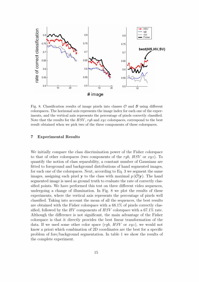
Fig. 8. Classification results of image pixels into classes O and B using differentcolorspaces. The horizonal axis represents the image index for each one of the exper-iments, and the vertical axis represents the percentage of pixels correctly classified.Note that the results for the HSV , rgb and xyz colorspaces, correspond to the bestresult obtained when we pick two of the three components of these colorspaces.

7 Experimental Results

We initially compare the class discrimination power of the Fisher colorspaceto that of other colorspaces (two components of the rgb, HSV or xyz). Toquantify the notion of class separability, a constant number of Gaussians arefitted to foreground and background distributions of hand segmented images,for each one of the colorspaces. Next, according to Eq. 3 we segment the sameimages, assigning each pixel y to the class with maximal p (O|y). The handsegmented image is used as ground truth to evaluate the rate of correctly clas-sified points. We have performed this test on three different video sequences,undergoing a change of illumination. In Fig. 8 we plot the results of theseexperiments, where the vertical axis represents the percentage of pixels wellclassified. Taking into account the mean of all the sequences, the best resultsare obtained with the Fisher colorspace with a 68.1% of pixels correctly clas-sified, followed by the HV components of HSV colorspace with a 67.1% rate.Although the difference is not significant, the main advantage of the Fishercolorspace is that it directly provides the best linear transformation of thedata. If we used some other color space (rgb, HSV or xyz), we would notknow a priori which combination of 2D coordinates are the best for a specificproblem of fore/background segmentation. In table 1 we show the results ofthe complete experiment.

15

ColorspaceSeq.1 Seq.2 Seq.3 Mean

µ σ µ σ µ σ µ σ

Fisher 0.770 0.033 0.630 0.035 0.602 0.016 0.681 0.082

HV 0.748 0.025 0.609 0.035 0.624 0.016 0.671 0.071

HS 0.706 0.033 0.587 0.017 0.554 0.012 0.628 0.072

rg 0.709 0.031 0.589 0.018 0.545 0.014 0.627 0.076

xy 0.701 0.030 0.587 0.019 0.557 0.013 0.627 0.069

rb 0.705 0.033 0.589 0.017 0.546 0.009 0.626 0.074

gb 0.707 0.032 0.588 0.019 0.543 0.009 0.626 0.076

yz 0.694 0.032 0.583 0.020 0.557 0.013 0.622 0.067

xz 0.694 0.029 0.582 0.020 0.557 0.013 0.622 0.060

sv 0.628 0.045 0.571 0.022 0.561 0.013 0.592 0.045

Table 1Details of the results presented in Fig. 8. Each column represents the average overall images in a single experiment, and the last column is the mean of the threeexperiments. Every value, is the percentage of pixels correctly classified (mean andvariance), using a particular colorspace.

Next, two different experimental results are presented in order to illustratethe robustness of our system to several changing conditions of the environ-ment. Since the algorithm has been implemented in an interpretative language(MATLAB), we cannot discuss time performance issues, instead we focus onthe effectiveness of the method. Time performance depends linearly on thenumber of hypotheses used to estimate the color distributions.

In the first experiment, we track the boundary of a bending book (nonrigidmotion) in a video sequence where the lighting conditions change smoothlyfrom natural lighting to yellow lighting. In this case, as the displacement ofthe color distribution in color space was relatively small, we have used ‘only’5 hypotheses. Fig. 9 shows some frames of the sequence with the obtainedresults, the corresponding edge images and the a posteriori probability mapsof the foreground (the book). The sequence of edge images contains a lot ofnoisy boundaries that pose difficulties for the tracking process and for theadjustment of a deformable model to the edges of the object. However, theintegration with color information gives a first estimate of the object position,that allows us to eliminate many false edges and reduce the complexity of thedeformable model fitting procedure.

Whereas in the first experiment we demonstrate the need for integration of

16

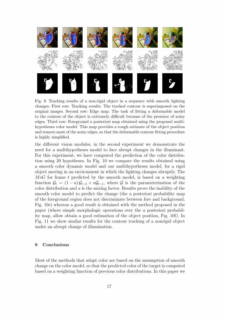
Fig. 9. Tracking results of a non-rigid object in a sequence with smooth lightingchanges. First row: Tracking results. The tracked contour is superimposed on theoriginal images. Second row: Edge map. The task of fitting a deformable modelto the contour of the object is extremely difficult because of the presence of noisyedges. Third row: Foreground a posteriori map obtained using the proposed multi-hypotheses color model. This map provides a rough estimate of the object positionand remove most of the noisy edges, so that the deformable contour fitting procedureis highly simplified.

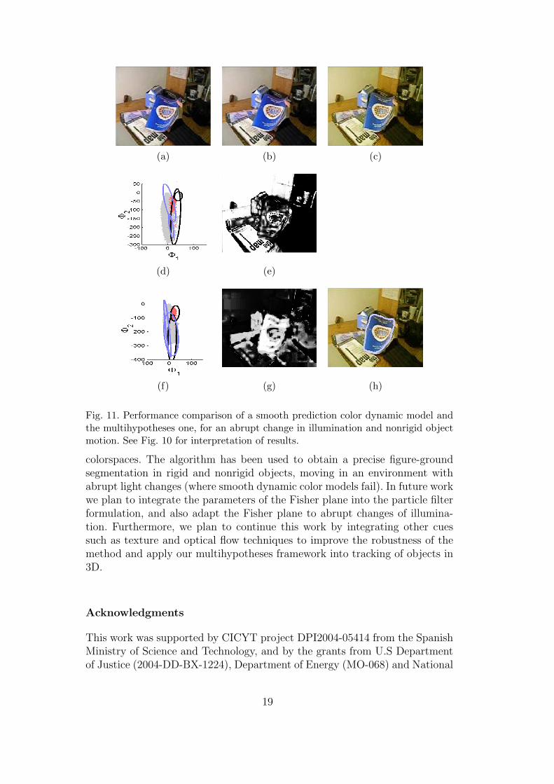
the different vision modules, in the second experiment we demonstrate theneed for a multihypotheses model to face abrupt changes in the illuminant.For this experiment, we have computed the prediction of the color distribu-tion using 20 hypotheses. In Fig. 10 we compare the results obtained usinga smooth color dynamic model and our multihypotheses model, for a rigidobject moving in an environment in which the lighting changes abruptly. TheMoG for frame t predicted by the smooth model, is based on a weightingfunction Gt = (1 − a)Gt−2 + aGt−1, where G is the parameterization of thecolor distribution and a is the mixing factor. Results prove the inability of thesmooth color model to predict the change (the a posteriori probability mapof the foreground region does not discriminate between fore and background,Fig. 10e) whereas a good result is obtained with the method proposed in thepaper (where simple morphologic operations over the a posteriori probabil-ity map, allow obtain a good estimation of the object position, Fig. 10f). InFig. 11 we show similar results for the contour tracking of a nonrigid objectunder an abrupt change of illumination.

8 Conclusions

Most of the methods that adapt color are based on the assumption of smoothchange on the color model, so that the predicted color of the target is computedbased on a weighting function of previous color distributions. In this paper we

17

(a) (b) (c)

(d) (e)

(f) (g) (h)

Fig. 10. Performance comparison of a smooth prediction color dynamic model andthe multihypotheses one, for an abrupt change in illumination and rigid objectmotion. (a),(b),(c) Frames t − 2, t − 1 and t are three consecutive images of thesequence. Note the abrupt change in illuminant between frames t− 1 and t. (d) El-lipses correspond to the foreground and background MoG predicted with a smoothcolor dynamic model. The real distributions of points in colorspace are also shown.(e) p (O|y) map obtained with the smooth model. There is no good discriminationbetween fore and background. (f) MoG of the best sample using the multihypothe-ses color dynamic model. (g) p (O|y) map obtained with this color model. Thereis good fore/background discrimination. (h) Tracking results obtained after usingp (O|y) to eliminate false edges from image and fitting a deformable contour.

have presented a method where this constraint is no longer needed, and thedynamic model is based on the formulation of multiple hypotheses about thenext state of the target color distribution. The best of these hypotheses is usedto obtain a rough estimate of the object position, and eliminate false and noisyedges, so that the task of fitting a deformable contour to the object bound-ary is considerably simplified. Reciprocally, this boundary is used to refinethe color estimation. Moreover, we propose the use of the Fisher colorspace,that has a better object/background discrimination performance than typical

18

(a) (b) (c)

(d) (e)

(f) (g) (h)

Fig. 11. Performance comparison of a smooth prediction color dynamic model andthe multihypotheses one, for an abrupt change in illumination and nonrigid objectmotion. See Fig. 10 for interpretation of results.

colorspaces. The algorithm has been used to obtain a precise figure-groundsegmentation in rigid and nonrigid objects, moving in an environment withabrupt light changes (where smooth dynamic color models fail). In future workwe plan to integrate the parameters of the Fisher plane into the particle filterformulation, and also adapt the Fisher plane to abrupt changes of illumina-tion. Furthermore, we plan to continue this work by integrating other cuessuch as texture and optical flow techniques to improve the robustness of themethod and apply our multihypotheses framework into tracking of objects in3D.

Acknowledgments

This work was supported by CICYT project DPI2004-05414 from the SpanishMinistry of Science and Technology, and by the grants from U.S Departmentof Justice (2004-DD-BX-1224), Department of Energy (MO-068) and National

19

Science Foundation (ACI-0313184).

References

[1] S.Birchfield, Elliptical head tracking using intensity gradients and colorhistograms, IEEE Conference on Computer Vision and Pattern Recognition,1998, pp. 232-237.

[2] M. Isard, A. Blake, Icondensaton: Unifiying low-Level and high-level trackingin a stochastic framework, Proceedings of the ECCV, 1996, pp. 893-908.

[3] G.D. Finlayson, B.V. Funt, K. Barnard, Color constancy under varyingillumination, Proceedings of the International Conference on Computer Vision,1995, pp. 720-725.

[4] L. Sigal, S. Sclaroff, V. Athitsos, Estimation and prediction of evolvingcolor distributions for skin, Segmentation under Varying Illumination. IEEEConference on Computer Vision and Pattern Recognition 2000, vol(2), pp.152-159.

[5] J. Yang, W. Lu, A. Waibel, Skin-color modeling and adaption, ProceedingsACCV, 1998, vol.2, pp.687-694.

[6] Y. Raja, S. McKenna, S. Gong, Colour model seleciton and adaption in dynamicscenes, Proceedings of the ECCV, 2000, vol.1, pp.460-475.

[7] K. Fukunaga, Introduction to statistical pattern recognition, second ed.,Academic Press, 1990.

[8] F. Moreno-Noguer, J. Andrade-Cetto, A. Sanfeliu, Fusion of color and shapefor object tracking under varying illumination, Proceedings IBPRIA, LNCS2652, Springer, 2003, pp.580-588.

[9] K. Nummiaro, E. Koller-Meier, L. Van Gool, An adaptive color-based particlefilter, Image and Vision Computing 2(1) (2003) 99-110.

[10] A. Blake, M. Isard, Active contours, Springer-Verlag, 1998.

[11] M. Kass, A. Witkin, D. Terzopoulos, Snakes: Active contour models. Int. J.Computer Vision (1) (1987) 321-331.

[12] R.O. Duda, P.E. Hart, Pattern recognition and scene analysis, Wiley, NewYork, 1973.

[13] M.A.T. Figueiredo, A.K. Jain, Unsupervised learning of finite mixture models,IEEE Trans. Pattern Anal. Mach. Intell. 24(3) (2002) 381-396.

[14] T. McInerney, D. Terzopoulos, Deformable models in medical image analysis:A survey, Medical Image Analysis 1(2) (1996) 91-108.

[15] C. Xu, J.L. Prince, Snakes, shapes, and gradient vector flow, IEEE Transactionson Image Processing 7(3) (1998) 359-369.

20