Embed Size (px)
Citation preview
Central California Ozone Study (CCOS)
Volume II:Field Operations Plan
Version 2May 31, 2000
CCOS Field Operations Plan Version 2: 5/31/00
ii
Central California Ozone Study – Volume IIField Operations Plan
Prepared by:
Eric Fujita, Robert Keislar, William Stockwell, Saffet Tanrikulu and Andrew RanzieriDan Freeman, John Bowen and Richard Tropp Planning and Technical Support DivisionDivision of Atmospheric Science California Air Resources BoardDesert Research Institute 2020 L Street2215 Raggio Parkway Sacramento, CA 95812Reno, NV 89512 www.arb.ca.gov
www.arb.ca.gov/ccaqs/ccos/ccos.htm
The CCOS Plan was prepared with extensive input from the CCOS Field Study Participants, TechnicalCommittee, Scientific Advisory Work Group, Meteorological Work Group, and Emission InventoryCoordination Group.
Technical Committee(Planning Subcommittee)
Andrew Ranzieri, California Air Resources BoardSaffet Tanrikulu, California Air Resources BoardRob DeMandel, Bay Area AQMDBruce Katayama, Sacramento Metropolitan AQMDEvan Shipp, San Joaquin Valley Unified APCDPhil Roth, EnvairJim Sweet, San Joaquin Valley Unified APCDBrigette Tollstrup, Sacramento Metropolitan AQMDSteve Ziman, Chevron Research and Technology
Scientific Advisory Work Group
Dan Chang, University of California, DavisDennis Fitz, UCR, CE-CERTRobert Harley, University of California, BerkeleyMike Kleeman, University of California, DavisGail Tonnesen, University of California, Riverside
Meteorological Work Group
Saffet Tanrikulu, California Air Resources BoardBob Keislar, Desert Research InstituteDavid Fairley, Bay Area AQMDTom Umeda, Bay Area AQMDEvan Shipp, San Joaquin Valley Unified APCDSteve Gouze, California Air Resources BoardBruce Katayama, Sacramento Metropolitan AQMDBrigette Tollstrup, Sacramento Metropolitan AQMDBob Noon, Monterey Bay Unified AQMD
Emission Inventory Coordination Group
Linda Murchison, California Air Resources BoardDale Shimp, California Air Resources BoardCheryl Taylor, California Air Resources BoardDennis Wade, California Air Resources BoardMichael Benjamin, California Air Resources BoardPhil Martien, Bay Area AQMDToch Mangat, Bay Area AQMDBruce Katayama, Sacramento Metropolitan AQMDBrigette Tollstrup, Sacramento Metropolitan AQMDHazel Hoffmann, San Joaquin Valley Unified APCDDave Jones, San Joaquin Valley Unified APCDTom Jordon, San Joaquin Valley Unified APCDScott Nestor, San Joaquin Valley Unified APCDStephen Shaw, San Joaquin Valley Unified APCDGretchen Bennett, Northern Sierra AQMDDick Johnson, Placer County APCDTom Roemer, San Luis Obispo County APCDLarry Green, Yolo-Solano AQMDNancy O’Connor, Yolo-Solano AQMDDave Smith, Yolo-Solano AQMDGordon Garry, Sacramento Area CoGGuido Franco, California Energy CommissionMorris Goldberg, U.S. EPA
CCOS Field Operations Plan Version 2: 5/31/00
iii
FIELD STUDY PARTICIPANTS
Technical CoordinationDon McNerny, California Air Resources BoardAndrew Ranzieri, California Air Resources BoardSaffet Tanrikulu, California Air Resources BoardEric Fujita, Desert Research Institute
Field Management and FacilitiesEric Fujita, Desert Research InstituteDan Freeman, Desert Research InstituteChuck McDade, ENSRDave Wright, AVES/ATC Associates, Inc.
Episode ForecastSaffet Tanrikulu, California Air Resources BoardEvan Shipp, San Joaquin Valley Unified APCDAvi Okin, Bay Area AQMDJohn Ching, Sacramento Metropolitan AQMDBob Keislar, Desert Research Institute
Supplemental Surface Air Quality OperationsJohn Bowen, Desert Research InstituteRichard Tropp, Desert Research InstituteBill Coulombe, Desert Research InstituteBill Stockwell, Desert Research InstituteDennis Fitz, UC Riverside, CE-CERTDon Lehrman, T&B SystemsRobert Harley, UC Berkeley
Nitrogen Species MeasurementsDennis Fitz, UC Riverside, CE-CERTKurt Burmiller, UC Riverside, CE-CERTJohn Collins, UC Riverside, CE-CERTClaudia Sauer, UC Riverside, CE-CERTJohn Pisano, UC Riverside, CE-CERTSusanne Hering, Aerosol Dynamics, Inc.
Volatile Organic Compound MeasurementsBarbara Zielinska, Desert Research InstituteJohn Sagebiel, Desert Research InstituteWendy Goliff, Desert Research InstituteRei Rasmussen, Biospheric Research CorporationKochy Fung, AtmAA
Supplemental Meteorological MeasurementsBill Neff, NOAAClark King, NOAAJerry Crescenti, NOAATom Strong, NOAATim Dye, Sonoma Technology, IncDon Lehrman, T&B SystemsJay Rosenthal, U.S. Navy
Airborne MeasurementsDon Blumenthal, Sonoma Technology, Inc.Jerry Anderson, Sonoma Technology, Inc.John Carroll, UC DavisAlan Dixon, UC DavisRoger Tanner, Tennessee Valley AuthorityRalph Valente, Tennessee Valley AuthorityRich Barchet, Pacific Northwest National LaboratoryShiyuan Zhnog, PNNLLeonard Barrie, PNNL
Quality Assurance AuditsDave Bush, Parsons Engineering ScienceBob Baxter, Parsons Engineering ScienceDave Wright, AVES/ATC Associates, Inc.Lin Linsey, Northwest Research Assoc., Inc.Mike Miguel, California Air Resources BoardDon Fitzell, California Air Resources BoardAvi Okin, Bay Area AQMD
Data Management and EvaluationGreg O’Brien, California Air Resources BoardLiz Niccum, T&B SystemsEric Fujita, Desert Research Institute
Sponsoring OrganizationsCalifornia Air Resources BoardCalifornia Energy CommissionBay Area Air Quality Management DistrictMendocino County Air Pollution Control DistrictSacramento Metropolitan AQMDSan Joaquin Unified Air Pollution Control DistrictSan Luis Obispo Air Pollution Control DistrictWestern States Petroleum Association
CCOS Field Operations Plan Version 2: 5/31/00
iv
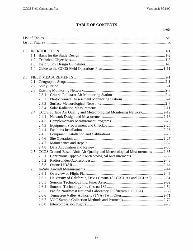
TABLE OF CONTENTSPage
List of Tables ............................................................................................................................... viiList of Figures ................................................................................................................................ix
1.0 INTRODUCTION ............................................................................................................... 1-11.1 Basis for the Study Design.......................................................................................... 1-21.2 Technical Objectives................................................................................................... 1-51.3 Field Study Design Guidelines.................................................................................... 1-91.4 Guide to the CCOS Field Operations Plan................................................................ 1-11
2.0 FIELD MEASUREMENTS ................................................................................................ 2-12.1 Geographic Scope ....................................................................................................... 2-12.2 Study Period................................................................................................................ 2-12.3 Existing Monitoring Networks.................................................................................... 2-3
2.3.1 Criteria Pollutant Air Monitoring Stations...................................................... 2-42.3.2 Photochemical Assessment Monitoring Stations ............................................ 2-42.3.3 Surface Meteorological Networks................................................................... 2-82.3.4 Solar Radiation Measurements...................................................................... 2-11
2.4 CCOS Surface Air Quality and Meteorological Monitoring Network...................... 2-122.4.1 Network Design and Measurements.............................................................. 2-132.4.2 Complementary Measurement Programs ...................................................... 2-232.4.3 Equipment Procurement and Checkout ......................................................... 2-252.4.4 Facilities Installation ..................................................................................... 2-262.4.5 Equipment Installation and Calibrations ....................................................... 2-262.4.6 Site Operations .............................................................................................. 2-272.4.7 Maintenance and Repair................................................................................ 2-322.4.8 Data Acquisition and Review........................................................................ 2-33
2.5 CCOS Ground-Based Aloft Air Quality and Meteorological Measurements ........... 2-352.5.1 Continuous Upper-Air Meteorological Measurements ................................. 2-352.5.2 Radiosondes/Ozonesondes............................................................................ 2-432.5.3 Ozone LIDAR ............................................................................................... 2-44
2.6 In-Situ Aircraft Measurements.................................................................................. 2-442.6.1 Overview of Flight Plans............................................................................... 2-462.6.2 University of California, Davis Cessna 182 (UCD #1 and UCD #2)............ 2-512.6.3 Sonoma Technology Inc. Piper Aztec........................................................... 2-522.6.4 Sonoma Technology Inc. Cessna 182 ........................................................... 2-522.6.5 Pacific Northwest National Laboratory Gulfstream 159 (G-1)..................... 2-632.6.6 Tennessee Valley Authority (TVA) Twin Otter............................................ 2-712.6.7 VOC Sample Collection Methods and Protocols.......................................... 2-722.6.8 Intercomparison Flights................................................................................. 2-73
CCOS Field Operations Plan Version 2: 5/31/00
v
TABLE OF CONTENTS (cont.)Page
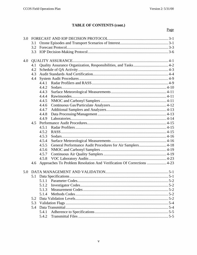
3.0 FORECAST AND IOP DECISION PROTOCOL.............................................................. 3-13.1 Ozone Episodes and Transport Scenarios of Interest.................................................. 3-13.2 Forecast Protocol......................................................................................................... 3-33.3 IOP Decision-Making Protocol ................................................................................... 3-6
4.0 QUALITY ASSURANCE................................................................................................... 4-14.1 Quality Assurance Organization, Responsibilities, and Tasks.................................... 4-24.2 Schedule of QA Activity ............................................................................................. 4-34.3 Audit Standards And Certification.............................................................................. 4-44.4 System Audit Procedures ............................................................................................ 4-9
4.4.1 Radar Profilers and RASS............................................................................... 4-94.4.2 Sodars............................................................................................................ 4-104.4.3 Surface Meteorological Measurements ......................................................... 4-114.4.4 Rawinsondes.................................................................................................. 4-114.4.5 NMOC and Carbonyl Samplers .................................................................... 4-114.4.6 Continuous Gas/Particulate Analyzers.......................................................... 4-124.4.7 Additional Samplers and Analyzers.............................................................. 4-134.4.8 Data Processing/Management ....................................................................... 4-134.4.9 Laboratories................................................................................................... 4-14
4.5 Performance Audit Procedures.................................................................................. 4-154.5.1 Radar Profilers .............................................................................................. 4-154.5.2 RASS............................................................................................................. 4-154.5.3 Sodars............................................................................................................ 4-164.5.4 Surface Meteorological Measurements ......................................................... 4-164.5.5 General Performance Audit Procedures for Air Samplers ............................ 4-184.5.6 NMOC and Carbonyl Samplers .................................................................... 4-194.5.7 Continuous Air Quality Samplers ................................................................. 4-194.5.8 VOC Laboratory Audits ................................................................................ 4-23
4.6 Approaches To Problem Resolution And Verification Of Corrections .................... 4-23
5.0 DATA MANAGEMENT AND VALIDATION................................................................. 5-15.1 Data Specifications...................................................................................................... 5-1
5.1.1 Parameter Codes.............................................................................................. 5-25.1.2 Investigator Codes........................................................................................... 5-25.1.3 Measurement Codes ........................................................................................ 5-25.1.4 Methods Codes................................................................................................ 5-2
5.2 Data Validation Levels................................................................................................ 5-25.3 Validation Flags .......................................................................................................... 5-45.4 Data Transmittal .......................................................................................................... 5-4
5.4.1 Adherence to Specifications............................................................................ 5-55.4.2 Transmittal Files ............................................................................................. 5-5
CCOS Field Operations Plan Version 2: 5/31/00
vi
TABLE OF CONTENTS (cont.)Page
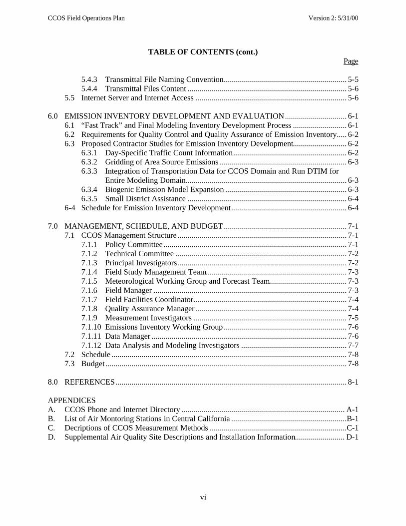
5.4.3 Transmittal File Naming Convention.............................................................. 5-55.4.4 Transmittal Files Content ................................................................................ 5-6
5.5 Internet Server and Internet Access ............................................................................ 5-6
6.0 EMISSION INVENTORY DEVELOPMENT AND EVALUATION............................... 6-16.1 “Fast Track” and Final Modeling Inventory Development Process ........................... 6-16.2 Requirements for Quality Control and Quality Assurance of Emission Inventory..... 6-26.3 Proposed Contractor Studies for Emission Inventory Development........................... 6-2
6.3.1 Day-Specific Traffic Count Information......................................................... 6-26.3.2 Gridding of Area Source Emissions................................................................ 6-36.3.3 Integration of Transportation Data for CCOS Domain and Run DTIM for
Entire Modeling Domain................................................................................. 6-36.3.4 Biogenic Emission Model Expansion ............................................................. 6-36.3.5 Small District Assistance ................................................................................ 6-4
6-4 Schedule for Emission Inventory Development.......................................................... 6-4
7.0 MANAGEMENT, SCHEDULE, AND BUDGET.............................................................. 7-17.1 CCOS Management Structure..................................................................................... 7-1
7.1.1 Policy Committee............................................................................................ 7-17.1.2 Technical Committee ...................................................................................... 7-27.1.3 Principal Investigators..................................................................................... 7-27.1.4 Field Study Management Team....................................................................... 7-37.1.5 Meteorological Working Group and Forecast Team....................................... 7-37.1.6 Field Manager ................................................................................................. 7-37.1.7 Field Facilities Coordinator............................................................................. 7-47.1.8 Quality Assurance Manager............................................................................ 7-47.1.9 Measurement Investigators ............................................................................. 7-57.1.10 Emissions Inventory Working Group.............................................................. 7-67.1.11 Data Manager .................................................................................................. 7-67.1.12 Data Analysis and Modeling Investigators ..................................................... 7-7
7.2 Schedule ...................................................................................................................... 7-87.3 Budget ......................................................................................................................... 7-8
8.0 REFERENCES.................................................................................................................... 8-1
APPENDICESA. CCOS Phone and Internet Directory .................................................................................. A-1B. List of Air Montoring Stations in Central California ..........................................................B-1C. Decriptions of CCOS Measurement Methods .....................................................................C-1D. Supplemental Air Quality Site Descriptions and Installation Information......................... D-1
CCOS Field Operations Plan Version 2: 5/31/00
vii
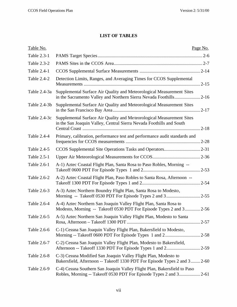
LIST OF TABLES
Table No. Page No.
Table 2.3-1 PAMS Target Species .......................................................................................... 2-6
Table 2.3-2 PAMS Sites in the CCOS Area............................................................................ 2-7
Table 2.4-1 CCOS Supplemental Surface Measurements .................................................... 2-14
Table 2.4-2 Detection Limits, Ranges, and Averaging Times for CCOS SupplementalMeasurements .................................................................................................... 2-15
Table 2.4-3a Supplemental Surface Air Quality and Meteorological Measurement Sitesin the Sacramento Valley and Northern Sierra Nevada Foothills...................... 2-16
Table 2.4-3b Supplemental Surface Air Quality and Meteorological Measurement Sitesin the San Francisco Bay Area........................................................................... 2-17
Table 2.4-3c Supplemental Surface Air Quality and Meteorological Measurement Sitesin the San Joaquin Valley, Central Sierra Nevada Foothills and SouthCentral Coast ..................................................................................................... 2-18
Table 2.4-4 Primary, calibration, performance test and performance audit standards andfrequencies for CCOS measurements ................................................................ 2-28
Table 2.4-5 CCOS Supplemental Site Operations Tasks and Operators............................... 2-31
Table 2.5-1 Upper Air Meteorological Measurements for CCOS......................................... 2-36
Table 2.6-1 A-1) Aztec Coastal Flight Plan, Santa Rosa to Paso Robles, Morning --Takeoff 0600 PDT For Episode Types 1 and 2................................................. 2-53
Table 2.6-2 A-2) Aztec Coastal Flight Plan, Paso Robles to Santa Rosa, Afternoon --Takeoff 1300 PDT For Episode Types 1 and 2.................................................. 2-54
Table 2.6-3 A-3) Aztec Northern Boundry Flight Plan, Santa Rosa to Modesto,Morning -- Takeoff 0530 PDT For Episode Types 2 and 3............................. 2-55
Table 2.6-4 A-4) Aztec Northern San Joaquin Valley Flight Plan, Santa Rosa toModesto, Morning -- Takeoff 0530 PDT For Episode Types 2 and 3............. 2-56
Table 2.6-5 A-5) Aztec Northern San Joaquin Valley Flight Plan, Modesto to SantaRosa, Afternoon – Takeoff 1300 PDT ............................................................... 2-57
Table 2.6-6 C-1) Cessna San Joaquin Valley Flight Plan, Bakersfield to Modesto,Morning -- Takeoff 0600 PDT For Episode Types 1 and 2.............................. 2-58
Table 2.6-7 C-2) Cessna San Joaquin Valley Flight Plan, Modesto to Bakersfield,Afternoon -- Takeoff 1330 PDT For Episode Types 1 and 2............................. 2-59
Table 2.6-8 C-3) Cessna Modified San Joaquin Valley Flight Plan, Modesto toBakersfield, Afternoon -- Takeoff 1330 PDT For Episode Types 2 and 3........ 2-60
Table 2.6-9 C-4) Cessna Southern San Joaquin Valley Flight Plan, Bakersfield to PasoRobles, Morning -- Takeoff 0530 PDT For Episode Types 2 and 3.................. 2-61
CCOS Field Operations Plan Version 2: 5/31/00
viii
LIST OF TABLES (cont.)
Table No. Page No.
Table 2.6-10 C-5) Cessna Southern San Joaquin Valley Flight Plan, Paso Robles toBakerfield, Afternoon – Takeoff 1330 PDT...................................................... 2-62
Table 2.6-11. Fresno area morning flight with low-level passes or spirals over key waypoints. ................................................................................................................. 2-64
Table 2.6.12 Fresno area afternoon flight with circuits above and within mixed layer.......... 2-65
Table 2.6-13. Western In-Flow Boundary flights..................................................................... 2-68
Table 2.6-14. PSC-FAT ferry flight ......................................................................................... 2-69
Table 2.6-15. FAT-PSC ferry flgiht ......................................................................................... 2-70
Table 2.6-16. Schedule of G-1 Activity in CCOS.................................................................... 2-70
Table 3.3-1 Chronology of Daily Forecast and IOP decisions................................................ 3-8
Table 4.2-1 Specifies the audit schedule for the ARB QA audit teams
(Van A and B). ..................................................................................................... 4-4
Table 4.2-1 ARB Audit Schedule – Van A............................................................................. 4-5
Table 4.2-2 ARB Audit Schedule – Van B ............................................................................. 4-6
Table 4.5-1. Summary of Meteorolgy Audit Methods and Criteria. ...................................... 4-24
Table 4.5-2. Linear Regression Criteria ................................................................................. 4-26
Table 5-1-1. Validation Flags ................................................................................................... 5-4
Table 5-2-1. FTP Transmittal file names.................................................................................. 5-6
Table 6.4-1 1999 Baseline Annual Average Emission Inventory Development..................... 6-5
Table 6.4-2 2000 Baseline Modeling Inventory Development ............................................. 6-10
Table 7.2-1 CCOS Schedule of Milestones............................................................................. 7-9
Table 7.3-1 CCOS Contracts and Other Costs ..................................................................... 7-10
Table 7.3-2 Equipment and Supplies from CCOS Equipment Budget and
Contingency Fund .............................................................................................. 7-11
Table 7.3-3 Equipment from CCOS Contracts and CRPAQS Equipment Budget............... 7-12
CCOS Field Operations Plan Version 2: 5/31/00
ix
LIST OF FIGURES
Figure No. Page No.
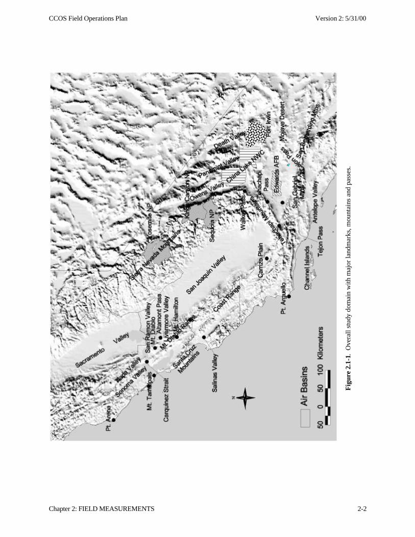
Figure 2.1-1 Overall study domain with major landmarks, mountains and passes. ................. 2-2
Figure 2.3-1. Central California surface meteorological networks and measurementlocations. ............................................................................................................. 2-9
Figure 2.3-2. Surface meteorological observables measured in the combined centralCalifornia meteorological network..................................................................... 2-10
Figure 2.4-1. Existing routine O3 and NOx monitoring sites.................................................. 2-19
Figure 2.4-2. CCOS supplemental air quality and meteorological monitoring sites andPhotochemical Assessment Monitoring Stations ............................................... 2-20
Figure 2.5-1. Upper air meteorological measurements during the summer campaign,including annual average study sites and NEXRAD (WSR-88D) profilers ...... 2-41
Figure 2.5-2. Upper air meteorological measurement network indicating operating agency. .2-42
Figure 2.6-1. Morning flight paths for CCOS IOPs................................................................. 2-48
Figure 2.6-2. Afternoon flight paths for CCOS IOPs ............................................................. 2-49
Figure 2.6-3. Afternoon flight path for post CCOS IOPs........................................................ 2-50
Figure 2.6-4. Fresno area flight patterns for morning flights with low-level passes orspirals at key way points (left) and afternoon flights with circuits aboveand within mixed layer (right)............................................................................ 2-66
Figure 2.6-5. Schematic representation of the flight patterns for the morning and afternoonwestern in-flow boundary flights. Fresno Air Terminal is at the far right,Monterey near center.......................................................................................... 2-67
Figure 2.6-6. Flight patterns for ferry flights between Pasco, WA (PSC) and Fresno ............ 2-71
CCOS Field Operations Plan Version 2: 5/31/00
Chapter 1: INTRODUCTION 1-1
1.0 INTRODUCTION
The Central California Ozone Study (CCOS) is a multi-year program of meteorologicaland air quality monitoring, emission inventory development, data analysis, and air qualitysimulation modeling. The goals of CCOS are to: 1) obtain suitable air quality, meteorologicaland emission databases to evaluate and improve air quality models for representing urban andregional-scale ozone episodes in central and northern California to meet the regulatoryrequirements for the state 1-hour and pending federal 8-hour ozone standards; 2) determine thecontributions of transport and locally generated ozone and the relative benefits of hydrocarbonand nitrogen oxides emission controls in upwind areas; and 3) assess the relative contributions ofozone generated from emissions in one air basin to state and federal exceedances in neighboringair basins. The modeling domain for CCOS covers all of central California and most of northernCalifornia, extending from the Pacific Ocean to east of the Sierra Nevada Mountains and fromRedding to the Mojave Desert. The selection of this study area reflects the regional nature of thestate 1-hour and federal 8-hour ozone exceedances, increasing urbanization of traditionally ruralareas, and a need to include all of the major flow features that affect air quality in centralCalifornia. The CCOS field measurement program will be conducted in the summer of 2000 inconjunction with the California Regional PM10/PM2.5 Air Quality Study (CRPAQS), a majorstudy of the origin, nature and extent of excessive levels of fine particles in central California(Watson et al., 1998).
The CCOS is a large-scale program involving many sponsors and participants. Threeentities are involved in the overall management of the Study. The San Joaquin Valleywide AirPollution Study Agency, a joint powers agency (JPA) formed by the nine counties in the Valley,directs the contracting aspects of the Study. A Policy Committee comprised of four votingblocks: State, local, and federal government, and the private sector, provides guidance on theStudy objectives and funding levels. The Policy Committee approves all proposal requests,contracts and reports and is responsible for fund raising. A Technical Committee parallels thePolicy Committee in membership and provides overall technical guidance on proposal requests,direction and progress of work, contract work statements, and reviews of all technical reportsproduced from the study. The technical committee comprises staff from the California AirResources Board, U.S. Environmental Protection Agency, the California Energy Commission,local air pollution control agencies, and industry, with technical input from a consortium ofuniversity researchers in the University of California System and the Desert Research Institute(DRI). On a day-to-day basis, the California Air Resources Board is responsible for managementof the Study.
The CCOS plan consists of a field study plan (Volume I) and this field operations plan(Volume II). These documents correspond to the two phases of the planning process for CCOS 1.The CCOS field study plan (Version 3: 11/24/99) is a product of regular meetings of the CCOSTechnical Committee and Working Groups over a six-month period and input from local airpollution control districts, academia, and industry reviewers on two earlier versions of the plan
1 Parallel efforts are also underway to develop a broad conceptual model of ozone formation in central Californiabased on San Joaquin Valley Air Quality Study and Atmospheric Utility Signatures, Predictions and ExperimentsRegional Model Adaptation Program (SARMAP) and other relevant studies and a “comprehensive” study plan thataddresses the long-term research needs related to the ozone problem in central California (Roth, 1999a and 1999b).
CCOS Field Operations Plan Version 2: 5/31/00
Chapter 1: INTRODUCTION 1-2
(released on 6/11/99 and 9/7/99). The field study plan describes the goals and technicalobjectives to be addressed by the study, and describes alternative experimental, modeling, anddata analysis approaches for addressing the study objectives. It presents a summary of the currentknowledge of meteorology, emissions, and chemical and physical processes that affect theformation and accumulation of ozone in northern and central California. It also reviews theresults from prior SAQM2 modeling by ARB, and identifies the remaining uncertainties and theirimplications for the design of the CCOS field measurement program. The plan describesrequirements for the modeling and data analysis approaches that are proposed to address CCOStechnical objectives and specifies measurements for modeling and data analysis. It considers themerits of alternative measurement approaches and explains the rationale and criteria formeasurement decisions. The field study plan is available in PDF format on the study web site athttp://www.arb.ca.gov/ccaqs/ccos/ccos.htm.
The field study plan served as the basis for contracts with measurement groups and fordeveloping the field operations plan for the summer 2000 field study. This field operations planspecifies the details of the field measurement program that will allow the field study plan to beexecuted with available resources. It identifies measurement locations, observables, andmonitoring methods, specifies data management and reporting conventions, and outlines theactivities needed to ensure data quality.
1.1 Basis for the Study Design
The goals of CCOS are to be met through a process that includes analysis of existingdata; execution of a large-scale field study in summer 2000 to acquire a comprehensive databaseto support modeling and data analysis; analysis of the data collected during the field study; andthe development, evaluation, and application of an air quality simulation model for northern andcentral California. Although air quality simulation modeling may be used to address CCOSgoals, past experience has demonstrated the need for thorough diagnostic analyses andcorroborative data analysis to assess the reliability of outputs from each part of the modelingsystem (i.e., emissions, meteorological, and air quality models). Corroborative data analysis isused to reinforce current understanding, identify gaps and improve the conceptual model ofozone formation, and to determine if measurement and modeling results are consistent with theconceptual model as revised by CCOS.
The reliability of model outputs is assessed through operational and diagnosticevaluations and application of alternative diagnostic tools. Operational evaluations consist ofcomparing concentration estimates from the model to ambient measurements. Diagnosticevaluations determine if the model is estimating ozone concentrations correctly for the rightreasons by assessing whether the physical and chemical processes within the model aresimulated correctly. This broad task also involves reconciliation of the corroborative dataanalysis results with modeling results. It includes evaluation of modeling uncertainties,processes, and assumptions and their effect on observed differences among model results,measurements, and data analysis results.
2 SARMAP Air Quality Model
CCOS Field Operations Plan Version 2: 5/31/00
Chapter 1: INTRODUCTION 1-3
Operational model evaluations will focus on the determination of the extent of agreementbetween simulated and measured concentrations of ozone and its precursors in their spatialdistribution and timing. The level of confidence that can be developed from this type ofevaluation increases with the number and variety of episodes and chemical species that areexamined. Measurements of the three-dimensional variations in ozone and ozone precursors alsoenhance the utility of the evaluations. Model simulations will be compared with airbornemeasurements of volatile organic compounds (total VOC, homologous groups, and lumpedclasses) along boundaries, above the mixed layer, and at the surface with measurements made atthe supplemental measurement sites. A similar comparison will be made for the measurements ofnitrogenous species concentrations. The temporal and spatial variability of the initial andboundary conditions will be evaluated to determine their effect on model output.
Diagnostic model evaluations examine the model’s representations of gas-phasechemistry, photolysis rates, treatment of advection, deposition rates and the treatment of subgridscale processes. The treatment of photolytic rate parameters will be evaluated by comparing themodel default values with measurements. Comparisons of calculated secondary chemical productconcentrations with measurements will be used to assess the chemical mechanisms. Otherexamples of chemical diagnostic tests include examining ratios of chemical species that aresensitive to specific processes within the model such as O3/NOy, O3/ NOz and comparingconcentration changes from weekdays to weekends. Process analysis (Jeffries and Tonnesen,1994) can be used to derive a detailed mass balance for each simulation. This allows thedetermination of the effect of each process on the concentrations of ozone and other airpollutants. Although it is not possible to use measurements to develop an independent,comprehensive mass balance throughout the study region, measurements (e.g., ratios of NO toNO2 or a highly reactive VOC to a less reactive VOC) can be used to check key parameterswithin the simulations. Alternatively model calculated parameters such as HO could be usedalong with measured mixing ratios of VOC to estimate VOC to NOx ratios. Both approachesshould provide strong tests of the conceptual model. Diagnostic evaluation of the transport ismore difficult but comparisons of the horizontal and vertical distributions of ozone and itsprecursors will be required. Another test to evaluate the transport would be to compare measuredand modeled fluxes of ozone and ozone precursors across interbasin transport corridors.
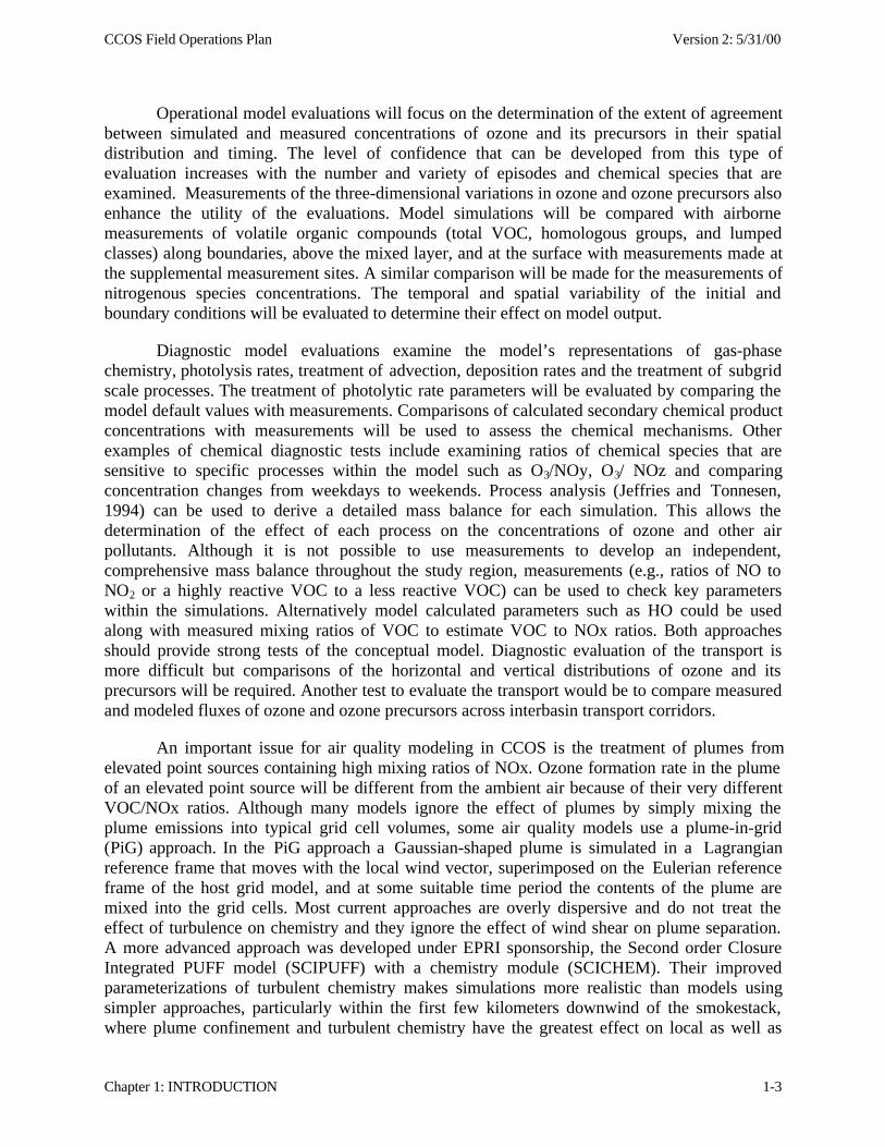
An important issue for air quality modeling in CCOS is the treatment of plumes fromelevated point sources containing high mixing ratios of NOx. Ozone formation rate in the plumeof an elevated point source will be different from the ambient air because of their very differentVOC/NOx ratios. Although many models ignore the effect of plumes by simply mixing theplume emissions into typical grid cell volumes, some air quality models use a plume-in-grid(PiG) approach. In the PiG approach a Gaussian-shaped plume is simulated in a Lagrangianreference frame that moves with the local wind vector, superimposed on the Eulerian referenceframe of the host grid model, and at some suitable time period the contents of the plume aremixed into the grid cells. Most current approaches are overly dispersive and do not treat theeffect of turbulence on chemistry and they ignore the effect of wind shear on plume separation.A more advanced approach was developed under EPRI sponsorship, the Second order ClosureIntegrated PUFF model (SCIPUFF) with a chemistry module (SCICHEM). Their improvedparameterizations of turbulent chemistry makes simulations more realistic than models usingsimpler approaches, particularly within the first few kilometers downwind of the smokestack,where plume confinement and turbulent chemistry have the greatest effect on local as well as
CCOS Field Operations Plan Version 2: 5/31/00
Chapter 1: INTRODUCTION 1-4
overall ozone production. The SCICHEM was evaluated favorably as part of the 1995Nashville/Middle Tennessee Ozone Study. Since the composition of the plumes will be differentfor central California, these new modules should be evaluate using the CCOS database.
In principle, well-performing air quality modeling systems have the ability to quantifylocal and transported contributions to ozone exceedances in a receptor area. However, many ofthe interbasin transport couples in the CCOS study region involve complex flow patterns withstrong terrain influences that are difficult to realistically simulate. The CCOS field campaignprovides routine and supplemental measurements at locations where transport can occur. Theproposed upper air network provides a “flux plane” method by which quantitative estimate ispossible, with suitable assumptions. In combination with modeling, data analyses can improvethe evaluation of modeling results and provide additional quantification of transportcontributions. Methods that should be applied include timing of ozone where morning peaksindicate fumigation of carry-over aloft, peaks near solar noon indicate possible localcontributions, and delayed peaks indicate transport, with later times corresponding to sitesfurther downwind along the transport path. Other methods include back trajectory wind analysisand examination of ratios of hydrocarbons of varying reactivity (i.e., xylenes-to-benzene ratio).In addition, vertical planes intersecting the profiler sites downwind of and perpendicular to thetransport path can be defined and provide estimates of transport through likely transportcorridors. The analyses use surface and aircraft measurements of pollutant concentrations andsurface, wind profiler, and aircraft meteorological data for volume flux estimations.
An important question for ozone control strategies is whether to focus on NOx or VOCcontrol. To choose the proper control strategy it is necessary to know if ozone production islimited in a location more by the NOx or VOC available. Models and measurements have beenapplied to answer this question. One of the methods would be to determine ozone isopleths frommeasurements for each site in an airshed but usually not enough data are available. Thereforeindicators for VOC or NOx limitation include ratios such as HNO3/H2O2 and other ratios havebeen applied to both measurements and models. Within CCOS, NOx and VOC limitation will beinvestigated through the use of measurements, indicators and modeling analysis.
One of the most important tests of model simulations is the ability to simulate accuratelyweekday-weekend differences in precursors and ozone. One of the most important applicationsof this test is that it helps to probe the relative sensitivity of ozone concentrations to VOC andNOx. Since the mid-1970’s it has been documented that ozone levels in California’s SouthCoast Air Basin (SoCAB) are higher on weekends than on weekdays, in spite of the fact thatozone pollutant precursors are lower on weekends than on weekdays (Elkus and Wilson, 1977;Horie et al., 1979; Levitts and Chock, 1975; Zeldin et al., 1989; Blier and Winer, 1998; andAustin and Tran, 1999). Similar effects have been observed in San Francisco (Altshuler et al.,1995) and in the northeastern cities of Washington D.C., Philadelphia, and New York (SAIC,1997). While a substantial “weekend effect” has been observed in these cities, the effect is lesspronounced in Sacramento (Austin and Tran, 1999), and is often reversed in Atlanta (Walker,1993) where VOC/NOx ratios are typically higher. Several of the above studies show that the“weekend effect” is generally less pronounced in downwind locations where ambient VOC/NOxratios are higher.
CCOS Field Operations Plan Version 2: 5/31/00
Chapter 1: INTRODUCTION 1-5
Understanding the response of ozone levels to specific changes in VOC or NOxemissions is a fundamental prerequisite to developing a cost-effective ozone abatement strategy.The varying emissions that occur between weekday and weekend periods provide a natural testcase for air quality simulation models. At the same time, the model performance and evaluationmust be accompanied by an evaluation of the accuracy of the temporal and spatial patterns ofprecursor emissions. With the questions that still remain regarding the accuracy of emissioninventories, the “weekend effect” emphasizes the need for observation-based data analysis toexamine the relationship between ambient O3 and precursor emissions. The results ofcorroborative data analyses need to be reconciled with model outputs taking into considerationthe various sources of uncertainties associated with both approaches.
The current conceptual model will be revisited and refined using the results yielded bythe foregoing data analyses. New phenomena, if they are observed, must be conceptualized sothat a mathematical model to describe them may be formulated and tested. The formulation,assumptions, and parameters in mathematical modules that will be included in the integrated airquality model will be examined with respect to their consistency with reality.
1.2 Technical Objectives
The study design and experimental approach for CCOS are defined in terms of specifictechnical objectives. A number of tasks are required to meet each of the technical objectives.These tasks are listed in this section and are described in greater detail in Sections 3 and 4 of thefield study plan (Fujita et al., 1999).
Preparation, Execution and Evaluation of Air Quality Simulation Modeling Systems (M)
Objective M-1. Apply air quality models for the attainment demonstration portion of the SIP forthe proposed 8-hour and state 1-hour ozone standards.
a. Select the most suitable modeling systems (for meteorology, emissions, and air quality)for representing photochemical air pollution in central and northern California. At leastone of the models selected should have the ability to simulate both ozone and fineparticles. Simulations with that model could be applied to both CRPAQS and CCOS.This will facilitate integration of results across both studies.
b. Analyze the data collected during the CCOS field measurement program and select aminimum of three ozone episodes to simulate.
c. Specify model domain boundaries, boundary conditions, initial conditions, chemicalmechanisms, aerosol module, plume-in-grid module, grid sizes, layers, and surfacecharacteristics.
d. Identify performance evaluation methods and performance measures, and specifymethods by which these will be applied.
e. Evaluate the results of the meteorological model.
CCOS Field Operations Plan Version 2: 5/31/00
Chapter 1: INTRODUCTION 1-6
f. Perform operational evaluation of the air quality model.
g. Evaluate and improve the performance of emissions, meteorological, and air qualitysimulations. Apply simulation methods to estimate ozone concentrations at receptor sitesand to test potential emissions reduction strategies.
h. Identify the limiting precursors of ozone and assess the extent to which reductions involatile organic compounds and nitrogen oxides, would be effective in reducing ozoneconcentrations.
Objective M-2. Determine the relative contributions of ozone generated from emissions in onebasin to federal and state exceedances in neighboring air basin.
a. Characterize the structure and evolution of the boundary layer and the nature of regionalcirculation patterns that determine the transport and diffusion of ozone and its precursorsin northern and central California.
b. Identify and describe transport pathways between neighboring air basins, and estimate thefluxes of ozone and precursors transported at ground level and aloft under differingmeteorological conditions. Reconcile results with flux plane measurements.
c. Determine the contribution of ozone generated from emissions in one basin to federal andstate exceedances in neighboring air basin through emission reduction sensitivityanalysis.
Objective M-3. Provide improve understanding of the role of thermal power plant plumes incontributing to regional air quality problems in central California.
a. Conduct measurements during CCOS Intensive Operational Periods (IOPs) in plumesfrom one or more power plants to allow reactive plume or plume-in-grid model to beevaluated.
b. Provide operational evaluation of a state-of-the-science reactive plume model componentusing data collected during the CCOS field study.
c. Using the modeling system developed by CCOS, provide a technical analysis appropriateto support the development of interbasin/intrabasin as well as interpollutant offset rulesthat could be applied to the central California region.
d. Run model simulations to estimate the air quality implications of different energypolicies.
Objective M-4. Assess the reliability associated with air quality model inputs and formulation,and reconcile model results with observation-based and other data analysis methods.
a. Perform diagnostic evaluation of model results.
CCOS Field Operations Plan Version 2: 5/31/00
Chapter 1: INTRODUCTION 1-7
b. Quantify the uncertainty of emissions rates, chemical compositions, locations, and timingof ozone precursors that are estimated by emission models.
c. Quantify the uncertainty of meteorological and air quality models in simulatingatmospheric transport, transformation, and deposition.
Data Analysis (D)
Objective D-1. Determine the accuracy, precision, validity, and equivalence of CCOS fieldmeasurements.
a. Evaluate the precision, accuracy, and validity of criteria pollutant data from routinemonitoring stations.
b. Evaluate the precision, accuracy, and validity of PAMS and CCOS supplemental VOCmeasurements and nitrogenous species measurements.
c. Evaluate the precision, accuracy, validity, and equivalence of routine network and CCOSsupplemental surface and upper-air meteorological data.
d. Evaluate the precision, accuracy, validity of data from instrumented aircraft andradiosonde/ozonesonde releases.
e. Evaluate the precision, accuracy, validity, and equivalence of routine and supplementalsolar radiation data.
Objective D-2. Determine the spatial, temporal, and statistical distributions of air qualitymeasurements to provide a guide to the database and aid in the formulation of hypotheses to betested by more detailed analyses.
a. Examine average diurnal changes of surface concentration data during episodic and non-episodic periods.
b. Examine spatial distributions of surface concentration data.
c. Examine statistical distributions and relationships among surface air qualitymeasurements.
d. Examine vertical distribution of concentrations from airborne measurements.
e. Examine the spatial and temporal distribution of solar radiation.
Objective D-3. Characterize meteorological transport phenomena and dispersion processes.
a. Examine the mechanisms for the movement of air into, out of, and between the differentair basins in both horizontal and vertical directions.
CCOS Field Operations Plan Version 2: 5/31/00
Chapter 1: INTRODUCTION 1-8
b. Determine occurrence, spatial extent, intensity, and variability of phenomena affectinghorizontal transport (low-level jet, slope flows, eddies, coastal meteorology and flowbifurcation) and vertical transport (convergence and divergence zones).
c. Characterize the depth, intensity, and temporal changes of the mixed layer andcharacterize mixing of elevated and surface emissions.
Objective D-4. Reconcile emissions inventory estimates with ambient measurements and “real-
a. Compare proportions of species measured in ambient air and those estimated by emissioninventories for reactive and nonreactive species.
b. Estimate source contributions by Chemical Mass Balance using measured and modeledambient VOC composition.
c. Conduct on-road remote sensing measurements of CO, HC, NOx and (PM if available) inSacramento, Fresno, and the San Francisco Bay Area, and evaluate the effects of cold-starts, grade and geographic distribution of high-emitting vehicles.
d. Reconcile on-road motor vehicle emission inventory estimates and fuel-based emissionsestimates.
e. Determine effects of meteorological variables on emissions rates.
f. Determine the detectability of day-specific emissions (e.g., fires) and variations inemissions between weekday and weekend.
Objective D-5. Characterize pollutant fluxes between upwind and receptor areas. Examine theorientations, dimensions, and locations of flux planes by using aircraft spiral and traverse data,and ground-based concentration data for VOCs, NOx, and O3 coupled with average wind speedsthat are perpendicular to the chosen flux planes.
a. Define the orientations, dimensions, and locations of flux planes.
b. Estimate the fluxes and total quantities of selected pollutants transported across fluxplanes. Test following hypotheses: 1) whether there is significant local generation ofpollutants; 2) whether there is significant dilution within or turbulent exchange throughthe top of the mixed layer; and 3) whether there is substantial transport or dilution owingto eddies, nocturnal jets, and upslope/downslope flows.
Objective D-6. Characterize chemical and physical interactions in the formation of ozone.
a. Examine VOC and nitrogen budgets as functions of location and time of day.
b. Reconcile the spatial, temporal, and chemical variations in ozone, precursor, and end-product concentrations with expectations from chemical theory.
CCOS Field Operations Plan Version 2: 5/31/00
Chapter 1: INTRODUCTION 1-9
c. Apply observation-based methods to determine where and when ozone concentrations arelimited by the availability of NOx or VOC.
d. Identify the composition and location of one or more power plant plumes and theirsurrounding air aloft so that the dispersion and chemical evolution of the plume(s) can beinferred.
Objective D-7. Characterize episodes in terms of emissions, meteorology, and air quality anddetermine the degree to which each intensive episode is a valid representation of commonlyoccurring conditions and its suitability for control strategy development.
a. Describe each intensive episode in terms of emissions, meteorology, and air quality.
b. Examine continuous meteorological and air quality data acquired for the entire studyperiod, and determine the frequency of occurrence of days which have transport andtransformation potential similar to those of the intensive study days. Generalize thisfrequency to previous years, using existing information for those years.
Objective D-8. Reformulate the conceptual model of ozone formation in the studydomain using the results yielded by the foregoing data analyses and modeling. Examine theformulation, assumptions, and parameters in mathematical modules in the air quality model withrespect to their consistency with reality.
1.3 Field Study Design Guidelines
The proposed measurement program incorporates the following design guidelines thatcombine technical, logistical and cost considerations, and lessons learned from similar studies.
1. CCOS is designed to provide the aerometric and emission databases needed to apply andevaluate atmospheric and air quality simulation models, and to quantify the contributionsof upwind and downwind air basins to exceedances of the federal 8-hour and state 1-hourozone standards in northern and central California. While urban-scale and regionalmodel applications are emphasized in this study, the CCOS database is also designed tosupport the data requirements of both modelers and data analysts. Air quality modelsrequire initial and boundary measurements for chemical concentrations. Meteorologicalmodels require sufficient three-dimensional wind, temperature, and relative humiditymeasurements for data assimilation. Data analysts require sufficient three-dimensionalair quality and meteorological data within the study region to resolve the main features ofthe flows and the spatial and temporal pollutant distributions. The data acquired foranalyses are used for diagnostic purposes to help identify problems with and to improvemodels.
2. Since episodes are caused by changes in meteorology, it is useful to document both themeteorology and air quality on non-episode days. For this reason, surface and upper airmeteorological data as well as surface air quality data for NOx and ozone will becontinuously collected during the entire summer of 2000. The database will be adequatefor modeling and a network of radar profilers will allow increased confidence in
CCOS Field Operations Plan Version 2: 5/31/00
Chapter 1: INTRODUCTION 1-10
assigning qualitative transport characterization (i.e., overwhelming, significant, orinconsequential) throughout the study period.
3. Many of the transport phenomena and important reservoirs of ozone and ozoneprecursors are found aloft. CCOS is designed to include extensive three-dimensionalmeasurements and simulations because the terrain in the study area is complex andbecause the flow field is likely to be strongly influenced by land-ocean interactions.Several upper air meteorological measurements are proposed at strategic locations toelucidate this flow field.
4. Although specific advances have been made in characterizing emissions from majorsources of precursor emissions, the accuracy of emission estimates for mobile, biogenicand other area sources at any given place and time remains poorly quantified. Ambientand source measurements (e.g., speciation profiles and remote sensing measurement ofon-road vehicles), with sufficient temporal and chemical resolution, are required toidentify and evaluate potential biases in emission inventory estimates.
5. Past studies document that the differences in temporal and spatial distributions ofprecursor emissions on weekdays and weekends alter the magnitude and distribution ofpeak ozone levels. Measurements are needed to evaluate model performance duringperiods that include weekends.
6. Measurements of documented quality and adequate sensitivity are needed along thewestern and northern boundaries of the modeling domain to adequately characterize thetemporal and spatial distributions of ambient background levels of ozone, volatile organiccompounds, and nitrogen oxides. Boundary conditions, particularly for formaldehyde,significantly affected model outputs in the SARMAP modeling resulting in over-prediction of ozone levels in the Bay Area. The same is true for NOx concentrations.SARMAP modeling shows that the western boundary has over 0.5 ppb of NO. Thesemoderate NO concentrations over the ocean appear to be due to transport from themodel’s boundary. Airborne measurements are needed far enough off shore to betterdefine the boundary conditions along the western boundary.
7. The measurements should be designed such that no single measurement system orindividual measurement is critical to the success of the program. The measurementnetwork should be dense enough that the loss of any one instrument or sampler will notsubstantially change analysis or modeling results. The study should be designed suchthat a greater number of intensive days than minimally necessary for modeling areincluded. This helps minimize the influence of atypical weather during the field programand decreases the probability of equipment being broken or unavailable on a day selectedfor modeling. Most measurements should be consistent in location and time for allintensive study days and during the entire study period (i.e., no movement ofmeasurements). In this way, one day can be compared to another. Continuousmeasurements should be designed to make use of the existing monitoring networks to theextent possible.
CCOS Field Operations Plan Version 2: 5/31/00
Chapter 1: INTRODUCTION 1-11
8. For model evaluation, it is desirable to have measurement stations along the line runningfrom the San Francisco Bay Area through Sacramento to the foothills of the SierraNevada and along the San Joaquin valley. The model predicts that ozone concentrationsshow strong variations over this region due to transport, deposition and chemistry.Measurement stations to measure ozone concentrations and the concentrations ofprecursors and other photochemical products placed along the west–east line will help todetermine if the models represent a scientifically reasonable description of ozoneformation and transport. The same can be said of an array of measurements through theSan Joaquin valley.
9. It is also important to have measurement stations to the north and south of theSacramento area because of the bifurcation in typical meteorological situations, where theflow fields from the west diverges toward the north and south. The ozone concentrationsshow several ozone hot spots one directly east of the San Francisco Bay Area with twomore directly to the north and south. Measurements to the north and south in this areawill help determine if the model predicted patterns are real. High ozone concentrationsalong and directly east and south of the San Joaquin valley. Measurement stations arerequired in this area as well.
10. The SAQM model predicts a rather complex vertical structure in ozone concentrations.The vertical structure of ozone concentrations along a north–south cross-section throughthe center of central California near Sacramento show that ozone is lost and transportedto the north and south leaving an arc of ozone that extends aloft and to the east and westby midnight. The vertical structure of the ozone concentrations along the west–east crosssection through central California along the line running from the San Francisco BayArea through Sacramento to the foothills of the Sierra Nevada is similar in its overallbehavior to the north–south line. The plots show evidence of transport of ozone and NOxfrom the west to the east. Ozone is lost in the lower levels and remains relatively highaloft as the time progresses from noon to midnight. Some of the parcels of high ozone areseen to travel from west to east in this sequence. Ozonesondes near San Francisco andSacramento and aircraft measurements of ozone over the Sierra Nevada foothills and thewestern boundary are required to observe this complex ozone structure predicted by themodels.
1.4 Guide to the CCOS Field Operations Plan
This field operations plan specifies the details of the field measurement program that willallow the field study plan to be executed with available resources. It identifies measurementlocations, observables, and monitoring methods, specifies data management and reportingconventions, and outlines the activities needed to ensure data quality. Section 2 specifies theCCOS measurement parameters, methods, locations, averaging times, calibration methods.Section 3 describes the meteorological conditions associated with ozone episodes and transportscenarios of interests, and specifies the daily forecast and intensive operational period (IOP)decision-making protocols. Sections 4 and 5 describe the quality assurance and data managementactivities for the study, respectively. Section 6 summarizes the efforts to develop a temporallyand spatially resolved emission inventory for the CCOS modeling domain, and Section 7specifies the program schedule and budget.
CCOS Field Operations Plan Version 2: 5/31/00
Chapter 2: FIELD MEASUREMENTS 2-1
2.0 CCOS FIELD MEASUREMENTS
Data requirements for CCOS are determined by the need to drive and evaluate theperformance of modeling systems, which include three components. A meteorological modelprovides winds fields, vertical profiles of temperature and humidity, and other physicalparameters in a gridded structure. Emissions inventory and supporting models provide griddedemissions for anthropogenic area and point sources and natural emissions. An air quality modelsimulates the chemical and physical processes involved in the formation and accumulation ofozone. In evaluating modeling system performance, the primary concern is replicating thephysical and chemical processes associated with actual ozone episodes. This necessitates thecollection of suitable meteorological, emissions, and air quality data that pertain to theseepisodes. The data requirements of CCOS are also driven by a need for complementary,independent and corroborative data analysis so that modeling results can be compared to currentconceptual understanding of the phenomena replicated by the model.
2.1 Geographic Scope
Central California is a complex region for air pollution, owing to its proximity to thePacific Ocean, its diversity of climates, and its complex terrain. Figure 2.1.1 show the overallstudy domain with major landmarks, mountains and passes. The CCOS domain includes most ofnorthern California and all of central California. The northern boundary extends north ofRedding and provides representation of the entire Central Valley of California. The westernboundary extends approximately 200 km west of San Francisco and allows the meteorologicalmodel to use mid-oceanic values for boundary conditions. The southern boundary extends belowSanta Barbara and into the South Coast Air Basin. The eastern boundary extends past Barstowand includes a large part of the Mojave Desert and all of the southern Sierra Nevada. The BayArea, southern Sacramento Valley, San Joaquin Valley, central portion of the Mountain CountiesAir Basin (MCAB), and the Mojave Desert are currently classified as nonattainment for thefederal 1-hour ozone NAS. With the exception of Plumas and Sierra Counties in the MCAB,Lake County, and the North Coast, the entire study domain is currently nonattainment for thestate 1-hour ozone standard. The Mojave Desert inherits poor air quality generated in the otherparts of central and southern California.
2.2 Study Period
The CCOS field measurement program will be conducted during a four-month periodfrom 6/1/00 to 9/30/00. A network of upper-air meteorological monitoring stations willsupplement the existing routine meteorological and air quality monitoring network in order toidentify and characterize meteorological conditions that are conducive to ozone formation duringthis four-month period. Supplemental air quality measurements will be made during a three-month period from 6/15/00 to 9/15/00 (study period), which corresponds to the majority ofelevated ozone levels observed in northern and central California during previous years.Continuous surface and upper-air meteorological measurements and surface air quality
CCOS Field Operations Plan Version 2: 5/31/00
Chapter 2: FIELD MEASUREMENTS 2-2
Fig
ure
2.1-
1. O
vera
ll st
udy
dom
ain
with
maj
or la
ndm
arks
, mou
ntai
ns a
nd p
asse
s.
CCOS Field Operations Plan Version 2: 5/31/00
Chapter 2: FIELD MEASUREMENTS 2-3
measurements of O3 NO, NOx or NOy1 will be made hourly throughout the study period in orderto provide sufficient input data to model any day during the study period. These measurementsare made in order to assess the representativeness of the episode days, to provide information onthe meteorology and air quality conditions on days leading up to the episodes, and to assess themeteorological regimes and transport patterns which lead to ozone episodes.
Additional continuous surface air quality measurements will be made at several sitesduring a shorter two-month study period from 7/6/00 to 9/2/00 (primary study period). Thesemeasurements include nitrogen dioxide (NO2), peroxyacetylnitrate (PAN) and otherperoxyacylnitrates (PAcN), particulate nitrate (NO3
-), formaldehyde (HCHO), and speciatedvolatile organic compounds (automated gas chromatography with ion-trap mass spectrometer) 2.These measurements allow detailed examination of the diurnal, day-to-day, and day-of-the-weekvariations in carbon and nitrogen chemistry at transport corridors and at locations downwind ofthe San Francisco Bay Area, Sacramento, Fresno, and Bakersfield where ozone formation maybe either VOC- or NOx-limited depending upon time of day and pattern of pollutant transport.These data support operational and diagnostic model evaluations, evaluations of emissioninventories, and corroborative observation-based data analyses.
Additional data will be collected during ozone episodes (intensive operational periods,IOPs) to better understand the dynamics and chemistry of the formation of high ozoneconcentrations. The budget for CCOS allows for up to 15 days total for episodic measurements.With an average episode of three to four days, four to five episodes are likely. Thesemeasurements include instrumented aircraft, speciated VOC, and radiosonde measurements,which are labor intensive and require costly expendables or laboratory analyses. IOPs will beforecasted during periods that correspond to categories of meteorological conditions calledscenarios, which are associated with ozone episodes and ozone transport in northern and centralCalifornia. These intensive measurements will be made on days leading up to and during ozoneepisodes and during specific ozone transport scenarios. Forecast and decision protocols aredescribed in Section 2. The IOP measurements are needed for operational and diagnostic modelevaluation, to improve our conceptual understanding of the causes of ozone episodes in the studyregion and the contribution of transport to exceedances of federal and state ozone standards indownwind areas.
2.3 Existing Monitoring Networks
Field monitoring includes continuous measurements over several months and intensivestudies that are performed on a forecast basis during selected periods when episodes are mostlikely to occur. This section describes the existing routine air quality and meteorologicalmonitoring network in northern and central California, and the options for continuous andintensive air quality and meteorological measurements (surface and aloft) to be made duringCCOS.
1 Reactive oxidized nitrogen (NOy) include nitric oxide (NO), nitrogen dioxide (NO2), nitrous acid (HONO),peroxynitric acid (HNO4), nitrate radical (NO3), nitrate aerosol (NO3-), dinitrogen pentoxide (N2O5), nitric acid(HNO3), peroxyacetylnitrate (PAN) and other PAN analogues, and organic nitrates (ORNI).2 These instruments will be installed during a two-week period from 6/12/00 to 6/23/00. Data collection will beginfrom the date of installation, one to two weeks prior to start of the primary study period.
CCOS Field Operations Plan Version 2: 5/31/00
Chapter 2: FIELD MEASUREMENTS 2-4
2.3.1 Criteria Pollutant Air Monitoring Stations
The California Air Resources Board and local air pollution control districts currentlyoperate 185 air quality monitoring stations throughout northern and central California. Of theactive sites, 130 measure ozone and 76 measure NOx. Carbon monoxide and hydrocarbons aremeasured at 57 and 11 sites, respectively. Data from these sites are routinely acquired andarchived by the ARB and Districts. This extensive surface air quality monitoring networkprovides a substantial database for setting initial condition for the model, and for operationalevaluation of model outputs. ARB, in collaboration with the California air quality managementdistricts, is establishing the PM2.5 monitoring sites. The existing PM10 acquires filter samplesevery sixth day. Several of the PM10 sites have continuous monitors that measure hourly PM10
everyday. Watson et al. (1998) describes the PM measurement network.
2.3.2 Photochemical Assessment Monitoring Stations
Under Title I, Section 182, of the 1990 Amendments to the Federal Clean Air Act, theEPA proposed the implementation of a national network of enhanced ambient air monitoringstations. States with areas classified as serious, severe, or extreme for ozone attainment arerequired to establish photochemical assessment monitoring stations (PAMS) as par of their StateImplementation Plan. Each station measures speciated hydrocarbons and carbonyl compounds,ozone, oxides of nitrogen, and surface meteorological data. Additionally, each area must monitorupper air meteorology at one representative site.
The program was phased in over a five-year schedule, beginning in 1994 at a rate of atleast one station per year. A maximum of five PAMS sites are required in affected nonattainmentareas, depending on the population of the Metropolitan Statistical Area/ConsolidatedMetropolitan Statistical Area (MSA/CMSA) or nonattainment area, whichever is larger. PAMSnetworks are based on selection of an array of site locations relative to ozone precursor sourceareas and predominant wind directions associated with high ozone events. Specific monitoringobjectives associated with each of these sites result in four distinct site types.
Type 1 sites are established to characterize upwind background and transported ozoneand its precursor concentrations entering the area and to identify those areas that are subjected tooverwhelming transport. Type 1 sites are located in the predominant morning upwind directionfrom the local area of maximum precursor emissions during the ozone season. Typically, Type 1sites will be located near the edge of the photochemical grid model domain in the predominantupwind direction from the city limits or fringe of the urbanized area.
Type 2 sites are established to monitor the magnitude and type of precursor emissions inthe area where maximum precursor emissions are expected. These sites also are suited for themonitoring of urban air toxic pollutants. Type 2 sites are located immediately downwind of thearea of maximum precursor emissions and are typically placed near the downwind boundary ofthe central business district. Additionally, a second Type 2 site may be required depending on thesize of the area, and will be placed in the second-most predominant morning wind direction.
CCOS Field Operations Plan Version 2: 5/31/00
Chapter 2: FIELD MEASUREMENTS 2-5
Type 3 sites are intended to monitor maximum ozone concentrations occurringdownwind from the area of maximum precursor emissions. Typically, Type 3 sites will belocated 10 to 30 miles downwind from the fringe of the urban area.
Type 4 sites are established to characterize the extreme downwind transported ozone andits precursor concentrations exiting the area and identify those areas that are potentiallycontributing to overwhelming transport in other areas. Type 4 sites are located in thepredominant afternoon downwind direction, as determined for the Type 3 site, from the localarea of maximum precursor emissions during the ozone season.
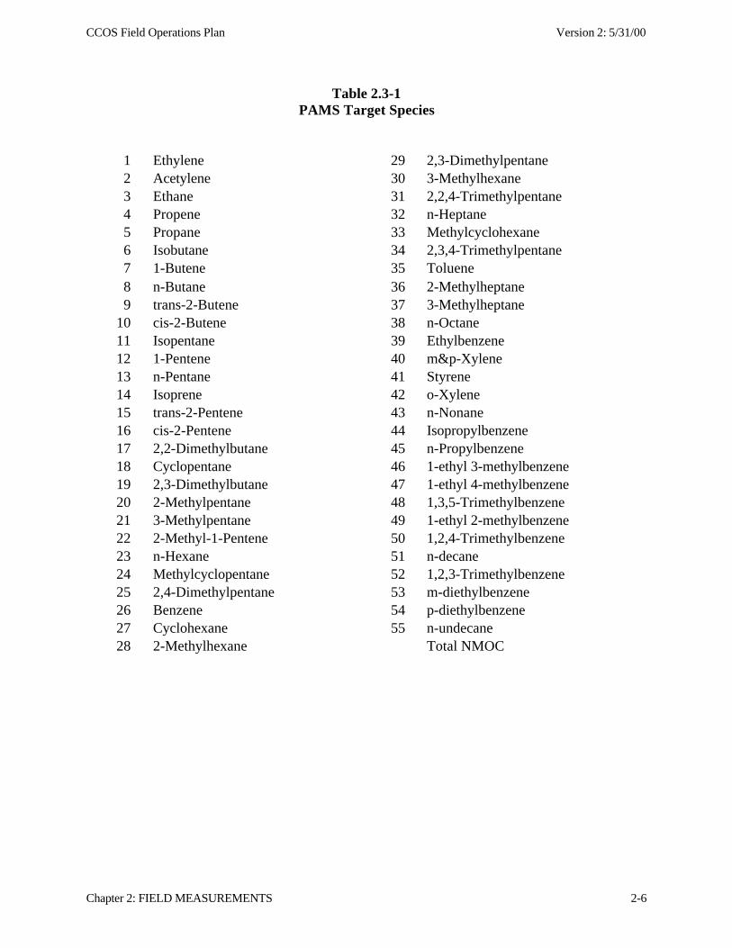
PAMS precursor monitoring is conducted annually in California during the peak ozoneseason (July, August and September). Eleven PAMS sites will be in operation during summer2000 (four in Sacramento County, four in Fresno County, and three in Kern County). EPAmethods TO-14 and TO-11 are specified by the EPA for sampling and analysis of speciatedhydrocarbons and carbonyl compounds, respectively (EPA, 1991). Table 2.3-1 contains theminimum list of targeted hydrocarbon species. For carbonyl compounds, state and localagencies are currently required to report only formaldehyde, acetaldehyde and acetone. The ARBand districts laboratories may be able to quantify and report several C3 to C7 carbonylcompounds that appear in the HPLC chromatograms.
Under the California Alternative Plan, four 3-hour samples (0000-0300, 0600-0900,1300-1600, and 1700-2000, PDT) are collected every third day during the monitoring period atall PAMS sites for speciated hydrocarbons and at Type 2 sites only for carbonyl compounds.These sampling periods are the same as the CCOS supplemental VOC sampling periods. Inaddition to the regularly scheduled measurements, samples are collected on a forecast basisduring up to five high-ozone episodes of at least two consecutive days. Episodic measurementsconsist of four samples per day (0600-0900, 0900-1200, 1300-1600, and 1700-2000, PDT) forspeciated hydrocarbons at all PAMS sites and for carbonyl compounds at Type 2 sites. Becausethe ARB laboratory has a limited number canisters and must recycle the them during the PAMSseason, a relaxation of the regularly scheduled PAMS sampling is necessary to accommodatemulti-day IOPs of three or more consecutive days. Instead of the sampling schedule in theCalifornia Alternative Plan, the U.S. Environmental Protection Agency has approved a requestby the ARB to modify the normal PAMS sampling schedule in order to accommodate moreepisodic sampling in coordination with the CCOS IOPs.
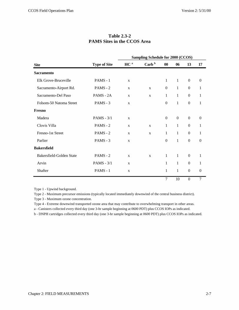
The implementation of PAMS by the local APCDs in central California during summer2000 is outlined in Table 2.3-2. The new sampling plan will retains only the 6-9 a.m (PDT)sample, every third day, to preserve the analysis of long-term trend. Up to 24 canister sampleswill be collected at PAMS sites in Central California during a maximum of three consecutiveIOP days during any one-week period. Table 2.3-2 shows the tentative allocation of the 24samples among the eleven PAMS sites in the CCOS domain. CCOS will also provide 100canisters to the PAMS program for contingency use.
CCOS Field Operations Plan Version 2: 5/31/00
Chapter 2: FIELD MEASUREMENTS 2-6
Table 2.3-1PAMS Target Species
1 Ethylene 29 2,3-Dimethylpentane2 Acetylene 30 3-Methylhexane3 Ethane 31 2,2,4-Trimethylpentane4 Propene 32 n-Heptane5 Propane 33 Methylcyclohexane6 Isobutane 34 2,3,4-Trimethylpentane7 1-Butene 35 Toluene8 n-Butane 36 2-Methylheptane9 trans-2-Butene 37 3-Methylheptane
10 cis-2-Butene 38 n-Octane11 Isopentane 39 Ethylbenzene12 1-Pentene 40 m&p-Xylene13 n-Pentane 41 Styrene14 Isoprene 42 o-Xylene15 trans-2-Pentene 43 n-Nonane16 cis-2-Pentene 44 Isopropylbenzene17 2,2-Dimethylbutane 45 n-Propylbenzene18 Cyclopentane 46 1-ethyl 3-methylbenzene19 2,3-Dimethylbutane 47 1-ethyl 4-methylbenzene20 2-Methylpentane 48 1,3,5-Trimethylbenzene21 3-Methylpentane 49 1-ethyl 2-methylbenzene22 2-Methyl-1-Pentene 50 1,2,4-Trimethylbenzene23 n-Hexane 51 n-decane24 Methylcyclopentane 52 1,2,3-Trimethylbenzene25 2,4-Dimethylpentane 53 m-diethylbenzene26 Benzene 54 p-diethylbenzene27 Cyclohexane 55 n-undecane28 2-Methylhexane Total NMOC
CCOS Field Operations Plan Version 2: 5/31/00
Chapter 2: FIELD MEASUREMENTS 2-7
Table 2.3-2PAMS Sites in the CCOS Area
Sampling Schedule for 2000 (CCOS)
Site Type of Site HC a Carb b 00 06 13 17
Sacramento
Elk Grove-Bruceville PAMS - 1 x 1 1 0 0
Sacramento-Airport Rd. PAMS - 2 x x 0 1 0 1
Sacramento-Del Paso PAMS - 2A x x 1 1 0 1
Folsom-50 Natoma Street PAMS - 3 x 0 1 0 1
Fresno
Madera PAMS - 3/1 x 0 0 0 0
Clovis Villa PAMS - 2 x x 1 1 0 1
Fresno-1st Street PAMS - 2 x x 1 1 0 1
Parlier PAMS - 3 x 0 1 0 0
Bakersfield
Bakersfield-Golden State PAMS - 2 x x 1 1 0 1
Arvin PAMS - 3/1 x 1 1 0 1
Shafter PAMS - 1 x 1 1 0 0
7 10 0 7
Type 1 - Upwind background.
Type 2 - Maximum precursor emissions (typically located immediately downwind of the central business district).
Type 3 - Maximum ozone concentration.
Type 4 - Extreme downwind transported ozone area that may contribute to overwhelming transport in other areas.
a - Canisters collected every third day (one 3-hr sample beginning at 0600 PDT) plus CCOS IOPs as indicated.
b - DNPH cartridges collected every third day (one 3-hr sample beginning at 0600 PDT) plus CCOS IOPs as indicated.
CCOS Field Operations Plan Version 2: 5/31/00
Chapter 2: FIELD MEASUREMENTS 2-8
Total nonmethane hydrocarbon (NMHC) concentrations are also measured by analysis ofthe canister samples by preconcentration direct injection flame ionization detection (PDFID).Total NMHC is measured by passing the air sample through a chromatographic column toseparate methane from other hydrocarbons and analyzing the bulk hydrocarbon sample by FID.In the FID, sample air is burned in a hydrogen flame creating a quantity of ions from thehydrogen molecules in the air sample. The ions conduct a small electrical current which ismeasured by an electrometer, which in turn produces an electronic signal proportional to thenumber of ions collected. Thus, the total hydrocarbon data are reported as parts per billioncarbon (ppbC). Total nonmethane hydrocarbon (NMHC) concentrations are monitoredcontinuously on an hourly basis at all Sacramento and San Joaquin Valley PAMS sites by eitherautomated-Preconcentration Direct Injection Flame Ionization Detection (PDFID) (e.g., Xontech850) or TEI 55C. Recent modifications of the TEI55C (Ventura option) provide improved limitof detection (from 150 ppbC to 75 ppbC).
2.3.3 Surface Meteorological Networks
The existing meteorological network in central California is extensive, but uncoordinatedamong the different agencies. Figure 2.3-1 shows the locations of surface meteorologicalmonitoring sites operated by the Air Resources Board (ARB), the Bay Area Air QualityManagement District (BAAQMD), the National Oceanic and Atmospheric Administration(NOAA), the California Irrigation Management Information Service (CIMIS), InteragencyMonitoring of PROtected Visual Environments (IMPROVE), the National Weather Service(NWS), Pacific Gas and Electric Company (PG&E), the U.S. Coast Guard, Remote AutomatedWeather Stations (RAWS) for fire fighting, and a few miscellaneous monitors. Wind speed anddirection, temperature, and relative humidity are the most common measurements. The networkof surface pressure and solar radiation measurements is also extensive. Three sites measureultraviolet radiation in the Sacramento Valley, in the San Joaquin Valley, and along the southcoast in Santa Barbara County. Figure 2.3-2 shows the surface meteorological observablesmeasured at each monitoring location, regardless of the network from which they are derived.The specific measurements at each site and the networks they belong to are documented inAppendix C of Watson et al., (1998).
Thuillier et al. (1994) document the methods used to acquire and report data in most ofthese networks with their similarities and differences. Wind speed measurements are taken atheights ranging from 2 m to 10 m agl at most sites and temperatures are measured by aspiratedand unaspirated thermometers. The major limitations of existing network instrumentation are: 1)wind thresholds of ~1 m/s for most instruments. The existing meteorological network will beaugmented with the CCOS supplemental sites described below. Ten meter meteorological towersat each of these sites will be equipped with low threshold (~0.3 m/s) wind sensors and highsensitivity relative humidity sensors. Section 10 describes the monitors available for thesemeasurements. With these supplemental measurements and surface measurements at the upperair sites, the existing surface monitoring network provides adequate coverage for the northernand central California study domain.
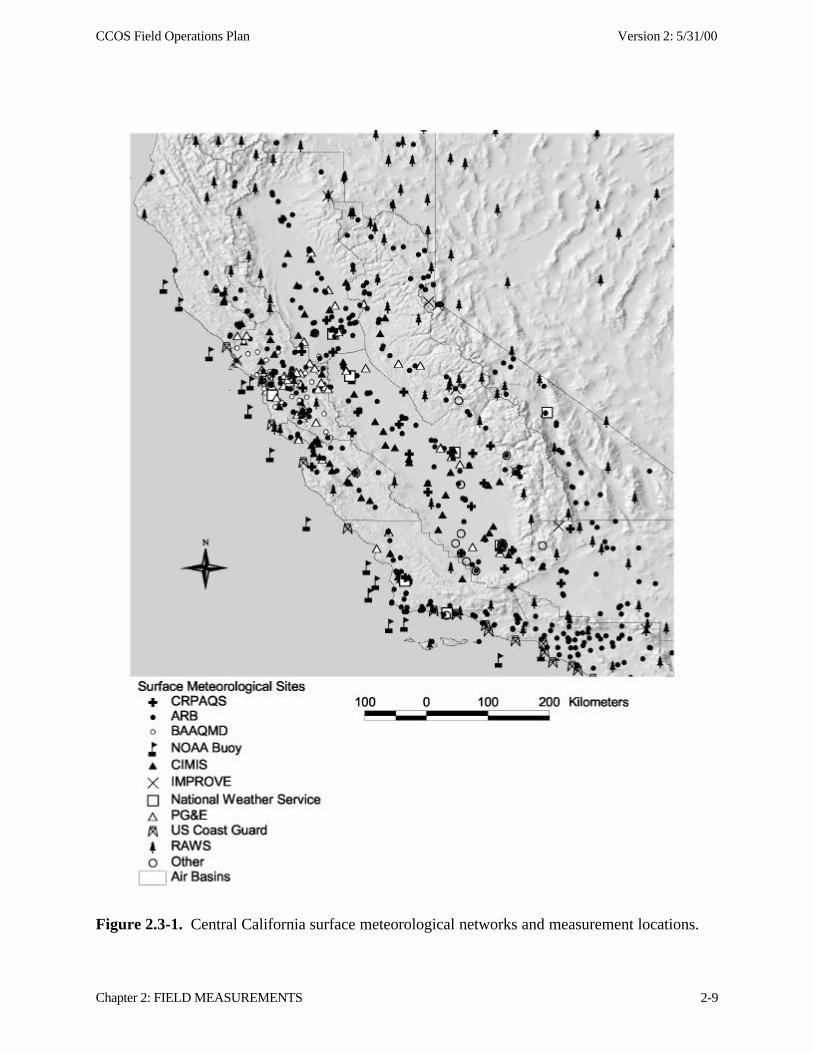
CCOS Field Operations Plan Version 2: 5/31/00
Chapter 2: FIELD MEASUREMENTS 2-9
Figure 2.3-1. Central California surface meteorological networks and measurement locations.
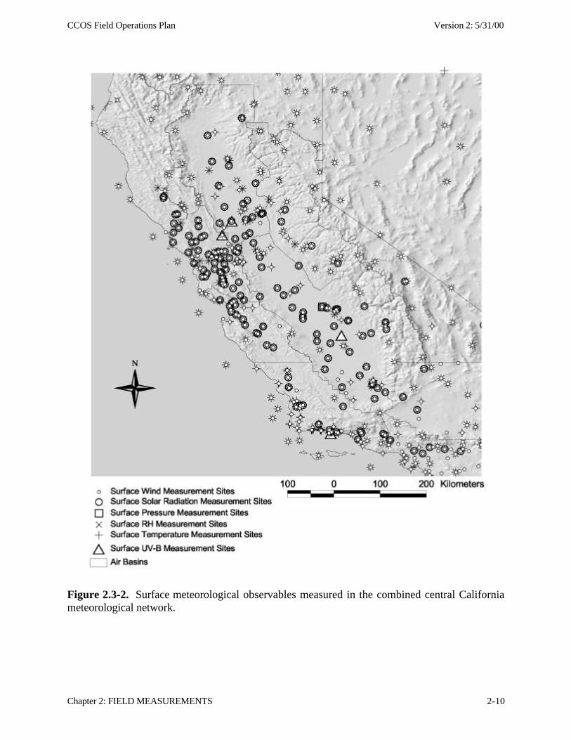
CCOS Field Operations Plan Version 2: 5/31/00
Chapter 2: FIELD MEASUREMENTS 2-10
Figure 2.3-2. Surface meteorological observables measured in the combined central Californiameteorological network.
CCOS Field Operations Plan Version 2: 5/31/00
Chapter 2: FIELD MEASUREMENTS 2-11
2.3.4 Solar Radiation Measurements
The US Department of Agriculture’s UVB Radiation Monitoring Program was initiatedin 1992, through a grant to Colorado State University, to provide information on thegeographical distribution and temporal trends of UVB radiation in the United States.Theclimatology network of the USDA-CSREES monitoring program is designed to provide anadequate density of measurement sites to establish the spatial and temporal characteristics ofUVB irradiance. The United States is divided into 26 regions of about equal area. Themeasurement sites are located primarily in rural areas near agricultural and forested regions. TheUS Department of Agriculture operates a UVB radiation measurement network with thefollowing two sites in California.
Station Name Closest town Longitude Latitude ElevationUC Davis ClimateStation
(Davis) 121.8 38.5 18
Desert Research andExtension Center
(Holtville) 115.4 32.8 -18
The US Department of Agriculture’s UVB Radiation Monitoring Program maintains onesite, near Davis, California (Latitude: 38.529, Longitude: 121.761). The site is operated by theUniversity of California at Davis. Co-location of one spectral radiometer for the measurement ofactinic flux to this site will provide significant advantage to CCOS. There are two existingMultifilter Rotating Shadowband Radiometers (MFRSR) at the USDA, Davis site. Ashadowband radiometer has a rotating metal band that periodically blocks the direct solar beamfrom entering the radiometer. This feature allows a measurement of the total horizontal, diffuseand direct normal components of the irradiance. One MFRS radiometer operates in the visibleregion and makes filter measurements at 415, 500, 610, 665, 862 and 940 nm and for the totalvisible radiation. The second MFRS operates in the UV and makes measurements at 300, 305.5,311.4, 317.6, 325.4, 332.4, 368 nm. The sampling time for the visible MFRSR is 15 seconds andthe sampling time for the ultraviolet MFRSR is 20 seconds however data from both MFRSR’sare stored as 3-minute averages. There are several other measurements that support the UVBradiation measurements at this site including sensors for UVA, UVB-1 and surface reflection andmeasurements of relative humidity, temperature and barometric pressure. Sample data from thissite may be obtained from:
http://uvb.nrel.colostate.edu/UVB/cgi_scripts/uvb_site_info_page.cgi?CA01&C.
Actinic flux in the troposphere depends most critically on the total ozone column, theaerosol loading, size and optical properties and the presence and characteristics of clouds. TheUV and visible MFRSR will allow the total ozone column and the aerosol characteristics to beestimated. The total ozone column measured by an UV-MFRSR was compared with standardBrewer and Dobson spectrophotometers. The average ratio of ozone retrieved by the UV-MFRSR to that of the Brewer was found to be 1.02 and to the Dobson 1.03. The USDA’s visibleand UV-MFRSRs data provides an estimate optical depths as a measure of the total aerosolloading. These data together with the actinic flux measurements will allow a direct evaluation ofthe photolysis rate parameters calculated for use in air quality models.

CCOS Field Operations Plan Version 2: 5/31/00
Chapter 2: FIELD MEASUREMENTS 2-12
The NOAA Integrated Surface Irradiance Study (ISIS) - A New Surface RadiationMonitoring Program. The Air Resources Laboratory (ARL) operates the NOAA nationalbroadband solar radiation network collecting data in both the visible and ultraviolet (UV-B)wavebands. ISIS operates at two levels: Level 1 monitors incoming radiation only and Level 2focuses on surface radiation balance. ISIS maintains a Level 1 site at Hanford, California in thecentral San Joaquin Valley. More detailed information is given in, "The NOAA IntegratedSurface Irradiance Study (ISIS) - A New Surface Radiation Monitoring Program", B.B. Hicks,J.J. DeLuisi, and D.R. Matt. Bull. Amer. Meteor. Soc., 77, 2857-2864.
High quality data is available from the NSF UV Monitoring Network that maintains a siteat San Diego approximately three miles from the Pacific Ocean. Although not in the CCOSdomain it may provide some useful information on the effect of marine clouds on UV irradiance.The facility is used for calibration and intercomparison of UV and visible radiometers. Thesystem has been operating since October 28, 1992. The use of UVB data from two other shouldbe considered, the EPA stratospheric UV network and the EPA Exposure network.
Existing Networks for Solar Radiation
Examination of network data for global solar radiation may give some help in estimatingthe photolysis rate parameters of nitrogen dioxide. The California Air Resources Board and theNREL operates sites that measure solar radiation.
The ARB operates five sites and local APCDs operate 31 sites. Hourly averages areobtained by a thermopile or pyranometer with and accuracy of ± 5 %. These data are availablefrom the Technical Support Division, Air Quality Data Branch, (916) 322-6076 or the U.S. EPAAerometric Information Retrieval System (AIRS).
The NREL National Solar Radiation Data Base (NSRDB) contains a total of 56 Primaryand 183 Secondary stations. The measurements made at these stations include global horizontalradiation in Wh/m2 , atmospheric pressure in millibars, direct normal radiation in Wh/m2, winddirection in increments of 10 degrees, diffuse horizontal radiation in Wh/m2, wind speed in m/s,extraterrestrial radiation (ETR) in Wh/m2, horizontal visibility in km, direct normal ETR inWh/m2Ceiling height in decameters, total sky cover in tenths, present weather, opaque sky coverin tenths, total precipitable water in mm, dry-bulb temperature in oC, aerosol optical depth, dew-point temperature in oC, snow depth in cm, relative humidity in percent, and number of dayssince last snowfall. The stations located in California are Daggett, Fresno, Los Angeles, SanDiego, and Santa Maria.
2.4 CCOS Surface Air Quality and Meteorological Monitoring Network
Supplemental air quality measurements are required at several existing monitoring sitesto increase the extent of chemical speciation and in key areas of the modeling domain whereroutine monitoring stations do not currently exist. Measurements of documented quality andadequate sensitivity are needed along the western boundary of the modeling domain toadequately characterize the temporal and spatial distributions of ambient background levels ofozone precursors because boundary conditions can significantly affected model outputs.Background sites intend to measure concentrations that are not influenced by northern and
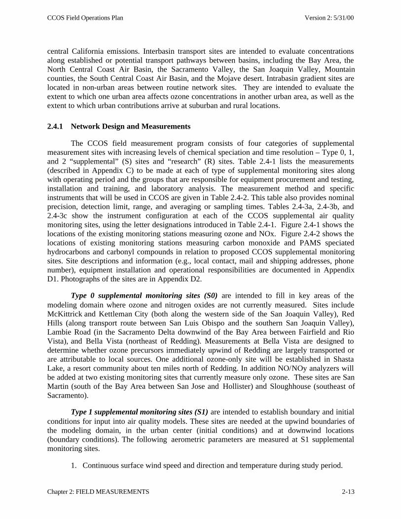
CCOS Field Operations Plan Version 2: 5/31/00
Chapter 2: FIELD MEASUREMENTS 2-13
central California emissions. Interbasin transport sites are intended to evaluate concentrationsalong established or potential transport pathways between basins, including the Bay Area, theNorth Central Coast Air Basin, the Sacramento Valley, the San Joaquin Valley, Mountaincounties, the South Central Coast Air Basin, and the Mojave desert. Intrabasin gradient sites arelocated in non-urban areas between routine network sites. They are intended to evaluate theextent to which one urban area affects ozone concentrations in another urban area, as well as theextent to which urban contributions arrive at suburban and rural locations.
2.4.1 Network Design and Measurements
The CCOS field measurement program consists of four categories of supplementalmeasurement sites with increasing levels of chemical speciation and time resolution – Type 0, 1,and 2 “supplemental” (S) sites and “research” (R) sites. Table 2.4-1 lists the measurements(described in Appendix C) to be made at each of type of supplemental monitoring sites alongwith operating period and the groups that are responsible for equipment procurement and testing,installation and training, and laboratory analysis. The measurement method and specificinstruments that will be used in CCOS are given in Table 2.4-2. This table also provides nominalprecision, detection limit, range, and averaging or sampling times. Tables 2.4-3a, 2.4-3b, and2.4-3c show the instrument configuration at each of the CCOS supplemental air qualitymonitoring sites, using the letter designations introduced in Table 2.4-1. Figure 2.4-1 shows thelocations of the existing monitoring stations measuring ozone and NOx. Figure 2.4-2 shows thelocations of existing monitoring stations measuring carbon monoxide and PAMS speciatedhydrocarbons and carbonyl compounds in relation to proposed CCOS supplemental monitoringsites. Site descriptions and information (e.g., local contact, mail and shipping addresses, phonenumber), equipment installation and operational responsibilities are documented in AppendixD1. Photographs of the sites are in Appendix D2.
Type 0 supplemental monitoring sites (S0) are intended to fill in key areas of themodeling domain where ozone and nitrogen oxides are not currently measured. Sites includeMcKittrick and Kettleman City (both along the western side of the San Joaquin Valley), RedHills (along transport route between San Luis Obispo and the southern San Joaquin Valley),Lambie Road (in the Sacramento Delta downwind of the Bay Area between Fairfield and RioVista), and Bella Vista (northeast of Redding). Measurements at Bella Vista are designed todetermine whether ozone precursors immediately upwind of Redding are largely transported orare attributable to local sources. One additional ozone-only site will be established in ShastaLake, a resort community about ten miles north of Redding. In addition NO/NOy analyzers willbe added at two existing monitoring sites that currently measure only ozone. These sites are SanMartin (south of the Bay Area between San Jose and Hollister) and Sloughhouse (southeast ofSacramento).
Type 1 supplemental monitoring sites (S1) are intended to establish boundary and initialconditions for input into air quality models. These sites are needed at the upwind boundaries ofthe modeling domain, in the urban center (initial conditions) and at downwind locations(boundary conditions). The following aerometric parameters are measured at S1 supplementalmonitoring sites.
1. Continuous surface wind speed and direction and temperature during study period.
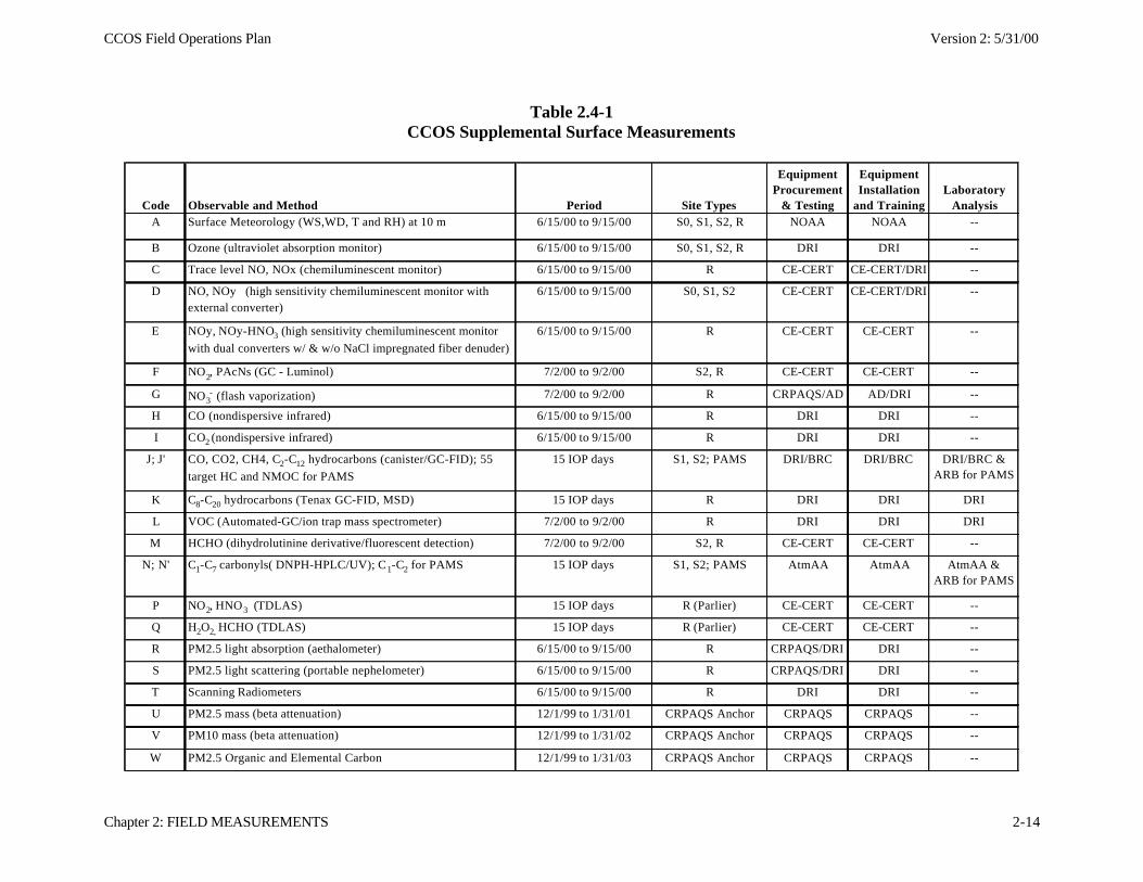
CCOS Field Operations Plan Version 2: 5/31/00
Chapter 2: FIELD MEASUREMENTS 2-14
Table 2.4-1CCOS Supplemental Surface Measurements
Code Observable and Method Period Site Types
Equipment Procurement
& Testing
Equipment Installation
and TrainingLaboratory
AnalysisA Surface Meteorology (WS,WD, T and RH) at 10 m 6/15/00 to 9/15/00 S0, S1, S2, R NOAA NOAA --
B Ozone (ultraviolet absorption monitor) 6/15/00 to 9/15/00 S0, S1, S2, R DRI DRI --
C Trace level NO, NOx (chemiluminescent monitor) 6/15/00 to 9/15/00 R CE-CERT CE-CERT/DRI --
D NO, NOy (high sensitivity chemiluminescent monitor with external converter)
6/15/00 to 9/15/00 S0, S1, S2 CE-CERT CE-CERT/DRI --
E NOy, NOy-HNO3 (high sensitivity chemiluminescent monitor
with dual converters w/ & w/o NaCl impregnated fiber denuder)
6/15/00 to 9/15/00 R CE-CERT CE-CERT --
F NO2, PAcNs (GC - Luminol) 7/2/00 to 9/2/00 S2, R CE-CERT CE-CERT --
G NO3- (flash vaporization) 7/2/00 to 9/2/00 R CRPAQS/AD AD/DRI --
H CO (nondispersive infrared) 6/15/00 to 9/15/00 R DRI DRI --
I CO2 (nondispersive infrared) 6/15/00 to 9/15/00 R DRI DRI --
J; J' CO, CO2, CH4, C2-C12 hydrocarbons (canister/GC-FID); 55
target HC and NMOC for PAMS
15 IOP days S1, S2; PAMS DRI/BRC DRI/BRC DRI/BRC & ARB for PAMS
K C8-C20 hydrocarbons (Tenax GC-FID, MSD) 15 IOP days R DRI DRI DRI
L VOC (Automated-GC/ion trap mass spectrometer) 7/2/00 to 9/2/00 R DRI DRI DRI
M HCHO (dihydrolutinine derivative/fluorescent detection) 7/2/00 to 9/2/00 S2, R CE-CERT CE-CERT --
N; N' C1-C7 carbonyls( DNPH-HPLC/UV); C1-C2 for PAMS 15 IOP days S1, S2; PAMS AtmAA AtmAA AtmAA & ARB for PAMS
P NO2, HNO3 (TDLAS) 15 IOP days R (Parlier) CE-CERT CE-CERT --
Q H2O2, HCHO (TDLAS) 15 IOP days R (Parlier) CE-CERT CE-CERT --
R PM2.5 light absorption (aethalometer) 6/15/00 to 9/15/00 R CRPAQS/DRI DRI --
S PM2.5 light scattering (portable nephelometer) 6/15/00 to 9/15/00 R CRPAQS/DRI DRI --
T Scanning Radiometers 6/15/00 to 9/15/00 R DRI DRI --
U PM2.5 mass (beta attenuation) 12/1/99 to 1/31/01 CRPAQS Anchor CRPAQS CRPAQS --
V PM10 mass (beta attenuation) 12/1/99 to 1/31/02 CRPAQS Anchor CRPAQS CRPAQS --
W PM2.5 Organic and Elemental Carbon 12/1/99 to 1/31/03 CRPAQS Anchor CRPAQS CRPAQS --
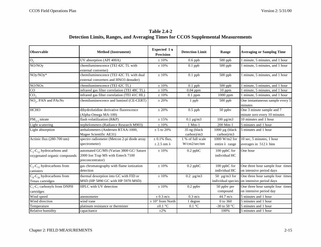
CCOS Field Operations Plan Version 2: 5/31/00
Chapter 2: FIELD MEASUREMENTS 2-15
Table 2.4-2Detection Limits, Ranges, and Averaging Times for CCOS Supplemental Measurements
Observable Method (Instrument) Expected 1 σ σ
PrecisionDetection Limit Range Averaging or Samplng Time
O3 UV absorption (API 400A) ± 10% 0.6 ppb 500 ppb 1 minute, 5 minutes, and 1 hour
NO/NOy chemiluminescence (TEI 42C TL with external converter)
± 10% 0.1 ppb 500 ppb 1 minute, 5 minutes, and 1 hour
NOy/NOy* chemiluminescence (TEI 42C TL with dual external converters and HNO3 denuder)
± 10% 0.1 ppb 500 ppb 1 minute, 5 minutes, and 1 hour
NO/NOx chemiluminescence (TEI 42C TL) ± 10% 0.1 ppb 500 ppb 1 minute, 5 minutes, and 1 hourCO infrared gas filter correlation (TEI 48C TL) ± 10% 0.04 ppm 10 ppm 1 minute, 5 minutes, and 1 hourCO2 infrared gas filter correlation (TEI 41C HL) ± 10% 0.1 ppm 1000 ppm 1 minute, 5 minutes, and 1 hour
NO2, PAN and PAcNs chemiluminescence and luminol (CE-CERT) ± 20% 1 ppb 500 ppb One instantaneous sample every 5 minutes
HCHO dihydrolutidine derivative fluorescence (Alpha-Omega MA-100)
± 20% 0.5 ppb 50 ppbv One 3 minute sample and 7 minute zero every 10 minutes
PM2.5 nitrate flash volatilization (R&P) ± 15% 0.1 µg/m3 100 µg/m3 10 minutes and 1 hour
Light scattering nephelometers (Radiance Research M903) ± 10% 1 Mm-1 200 Mm-1 5 minutes and 1 hourLight absorption aethalometers (Andersen RTAA-1000,
Magee Scientific AE31) ± 5 to 20% 35 ng (black
carbon)/m31000 µg (black
carbon)/m35 minutes and 1 hour
Actinic flux (280-700 nm) spectro radiometer (Metcon 2-pi diode array spectrometer)
± 0.1% flux,
± 2.5 nm λ1 % of full scale W/cm2/sec/nm
1000 W/m2 for
entire λ range
10 sec, 5 minutes, 1 hour
averages in 512 λ bins
C2-C12 hydrocarbons and
oxygenated organic compounds
automated GC/MS (Varian 3800 GC/ Saturn 2000 Ion Trap MS with Entech 7100 preconcentrator)
± 10% 0.2 ppbC 100 ppbC for individual HC
One hour
C2-C12 hydrocarbons from
canisters
gas chromatography with flame ionization detection
± 10% 0.2 ppbC 100 ppbC for individual HC
One three hour sample four times on intensive period days
C8-C20 hydrocarbons from
Tenax cartridges
thermal desorption into GC with FID or MSD (HP 5890 GC with HP 5970 MSD)
± 10% 0.2 µg/m3 50 µg/m3 for individual species
One three hour sample four times on intensive period days
C1-C7 carbonyls from DNPH
cartridges
HPLC with UV detection ± 10% 0.2 ppbv 50 ppbv per compound
One three hour sample four times on intensive period day
Wind speed anemometer ± 0.3 m/s 0.3 m/s 44.7 m/s 5 minutes and 1 hourWind direction wind vane ± 10° from North 1 degree 0 to 360 5 minutes and 1 hourTemperature platinum resistance or thermister ±0.1 °C 0.1 °C -30 to 50 °C 5 minutes and 1 hourRelative humidity capacitance ±2% 100% 5 minutes and 1 hour
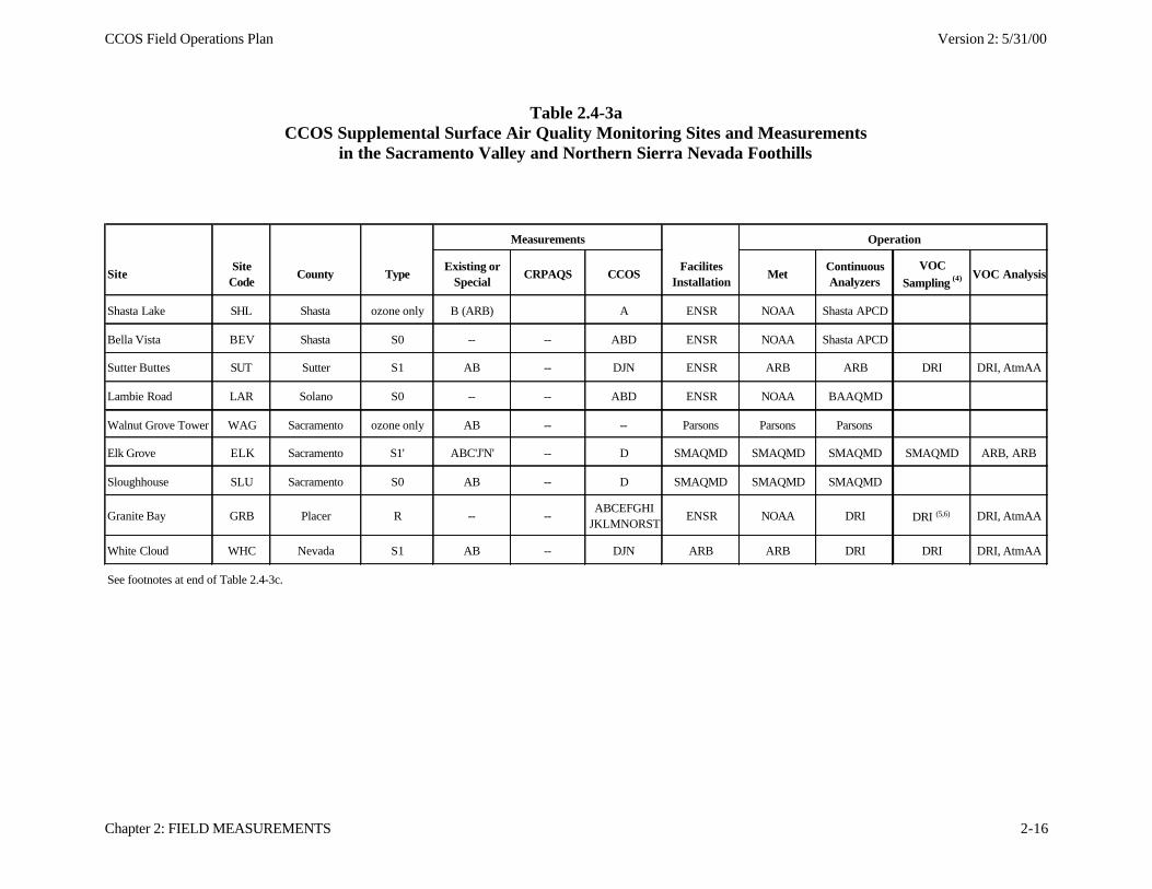
CCOS Field Operations Plan Version 2: 5/31/00
Chapter 2: FIELD MEASUREMENTS 2-16
Table 2.4-3aCCOS Supplemental Surface Air Quality Monitoring Sites and Measurements
in the Sacramento Valley and Northern Sierra Nevada Foothills
Measurements Operation
SiteSite
CodeCounty Type
Existing or Special
CRPAQS CCOSFacilites
InstallationMet
Continuous Analyzers
VOC
Sampling (4) VOC Analysis
Shasta Lake SHL Shasta ozone only B (ARB) A ENSR NOAA Shasta APCD
Bella Vista BEV Shasta S0 -- -- ABD ENSR NOAA Shasta APCD
Sutter Buttes SUT Sutter S1 AB -- DJN ENSR ARB ARB DRI DRI, AtmAA
Lambie Road LAR Solano S0 -- -- ABD ENSR NOAA BAAQMD
Walnut Grove Tower WAG Sacramento ozone only AB -- -- Parsons Parsons Parsons
Elk Grove ELK Sacramento S1' ABC'J'N' -- D SMAQMD SMAQMD SMAQMD SMAQMD ARB, ARB
Sloughhouse SLU Sacramento S0 AB -- D SMAQMD SMAQMD SMAQMD
Granite Bay GRB Placer R -- --ABCEFGHI
JKLMNORSTENSR NOAA DRI DRI (5,6) DRI, AtmAA
White Cloud WHC Nevada S1 AB -- DJN ARB ARB DRI DRI DRI, AtmAA
See footnotes at end of Table 2.4-3c.
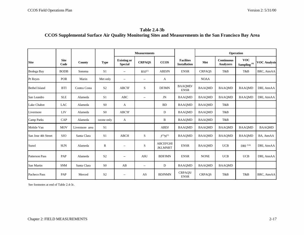
CCOS Field Operations Plan Version 2: 5/31/00
Chapter 2: FIELD MEASUREMENTS 2-17
Table 2.4-3bCCOS Supplemental Surface Air Quality Monitoring Sites and Measurements in the San Francisco Bay Area
Measurements Operation
SiteSite
CodeCounty Type
Existing or Special
CRPAQS CCOSFacilites
InstallationMet
Continuous Analyzers
VOC
Sampling (4) VOC Analysis
Bodega Bay BODB Sonoma S1 -- RSJ(1) ABDJN ENSR CRPAQS T&B T&B BRC, AtmAA
Pt Reyes POR Marin Met only -- -- A NOAA
Bethel Island BTI Contra Costa S2 ABC'H' S DFJMNBAAQMD/
ENSRBAAQMD BAAQMD BAAQMD DRI, AtmAA
San Leandro SLE Alameda S1 ABC -- JN BAAQMD BAAQMD BAAQMD BAAQMD DRI, AtmAA
Lake Chabot LAC Alameda S0 A BD BAAQMD BAAQMD T&B
Livermore LIV Alameda S0 ABC'H' D BAAQMD BAAQMD T&B
Camp Parks CAP Alameda ozone only A B BAAQMD BAAQMD T&B
Mobile Van MOV Livermore area S1 ABDJ BAAQMD BAAQMD BAAQMD BAAQMD BAAQMD
San Jose 4th Street SJO Santa Clara S1 ABCH S J(2)N(2) BAAQMD BAAQMD BAAQMD BAAQMD BA, AtmAA
Sunol SUN Alameda R -- SABCEFGHI JKLMNRT
ENSR BAAQMD UCB DRI (5,6) DRI, AtmAA
Patterson Pass PAP Alameda S2 -- ASU BDFJMN ENSR NONE UCB UCB DRI, AtmAA
San Martin SNM Santa Clara S0 AB -- D BAAQMD BAAQMD BAAQMD
Pacheco Pass PAP Merced S2 -- AS BDJNMNCRPAQS/
ENSRCRPAQS T&B T&B BRC, AtmAA
See footnotes at end of Table 2.4-3c.
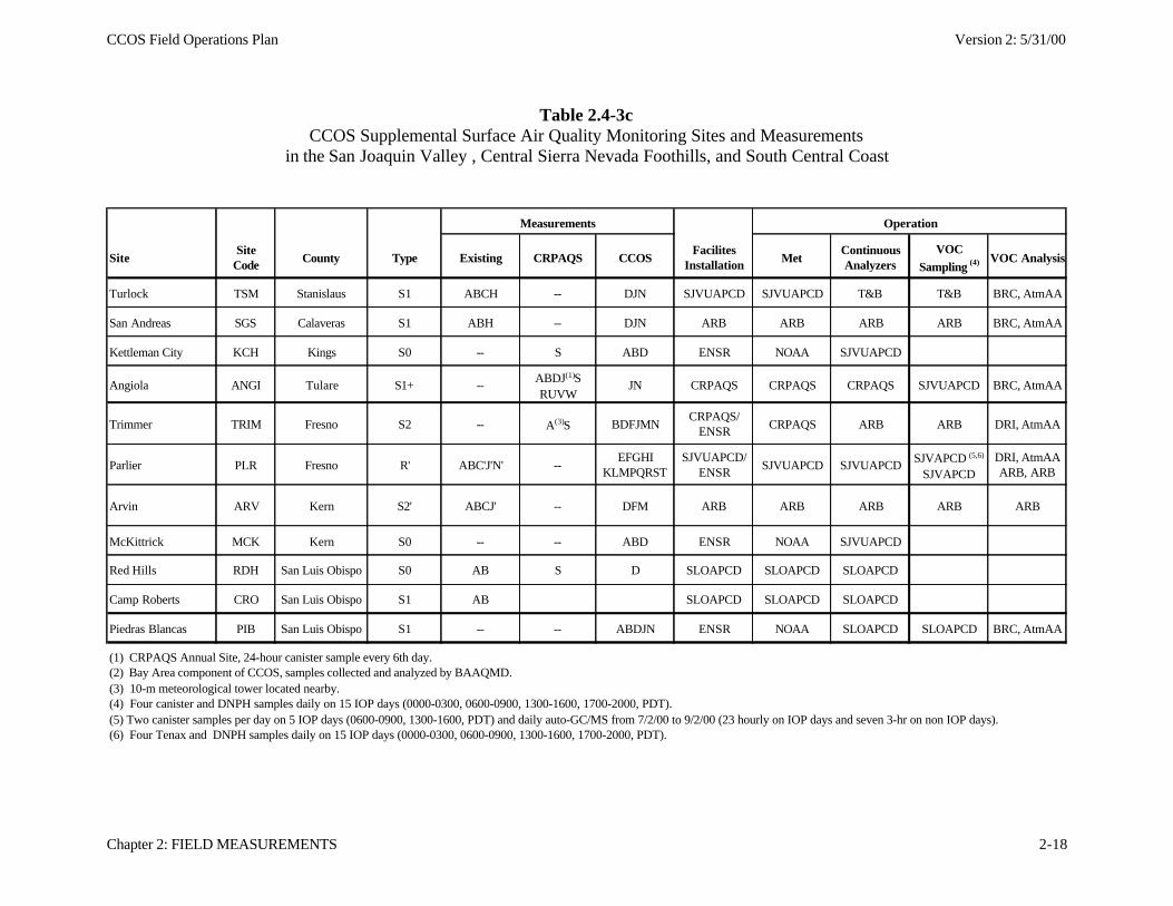
CCOS Field Operations Plan Version 2: 5/31/00
Chapter 2: FIELD MEASUREMENTS 2-18
Table 2.4-3cCCOS Supplemental Surface Air Quality Monitoring Sites and Measurements
in the San Joaquin Valley , Central Sierra Nevada Foothills, and South Central Coast
Measurements Operation
SiteSite
CodeCounty Type Existing CRPAQS CCOS
Facilites Installation
MetContinuous Analyzers
VOC
Sampling (4) VOC Analysis
Turlock TSM Stanislaus S1 ABCH -- DJN SJVUAPCD SJVUAPCD T&B T&B BRC, AtmAA
San Andreas SGS Calaveras S1 ABH -- DJN ARB ARB ARB ARB BRC, AtmAA
Kettleman City KCH Kings S0 -- S ABD ENSR NOAA SJVUAPCD
Angiola ANGI Tulare S1+ --ABDJ(1)S RUVW
JN CRPAQS CRPAQS CRPAQS SJVUAPCD BRC, AtmAA
Trimmer TRIM Fresno S2 -- A(3)S BDFJMNCRPAQS/
ENSRCRPAQS ARB ARB DRI, AtmAA
Parlier PLR Fresno R' ABC'J'N' --EFGHI
KLMPQRSTSJVUAPCD/
ENSRSJVUAPCD SJVUAPCD
SJVAPCD (5,6)
SJVAPCDDRI, AtmAA ARB, ARB
Arvin ARV Kern S2' ABCJ' -- DFM ARB ARB ARB ARB ARB
McKittrick MCK Kern S0 -- -- ABD ENSR NOAA SJVUAPCD
Red Hills RDH San Luis Obispo S0 AB S D SLOAPCD SLOAPCD SLOAPCD
Camp Roberts CRO San Luis Obispo S1 AB SLOAPCD SLOAPCD SLOAPCD
Piedras Blancas PIB San Luis Obispo S1 -- -- ABDJN ENSR NOAA SLOAPCD SLOAPCD BRC, AtmAA
(1) CRPAQS Annual Site, 24-hour canister sample every 6th day.(2) Bay Area component of CCOS, samples collected and analyzed by BAAQMD.(3) 10-m meteorological tower located nearby.(4) Four canister and DNPH samples daily on 15 IOP days (0000-0300, 0600-0900, 1300-1600, 1700-2000, PDT).(5) Two canister samples per day on 5 IOP days (0600-0900, 1300-1600, PDT) and daily auto-GC/MS from 7/2/00 to 9/2/00 (23 hourly on IOP days and seven 3-hr on non IOP days).(6) Four Tenax and DNPH samples daily on 15 IOP days (0000-0300, 0600-0900, 1300-1600, 1700-2000, PDT).
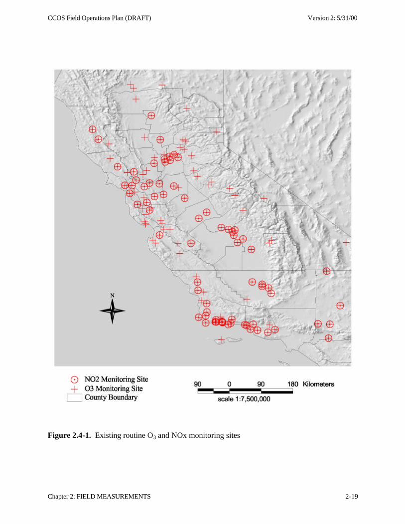
CCOS Field Operations Plan (DRAFT) Version 2: 5/31/00
Chapter 2: FIELD MEASUREMENTS 2-19
Figure 2.4-1. Existing routine O3 and NOx monitoring sites
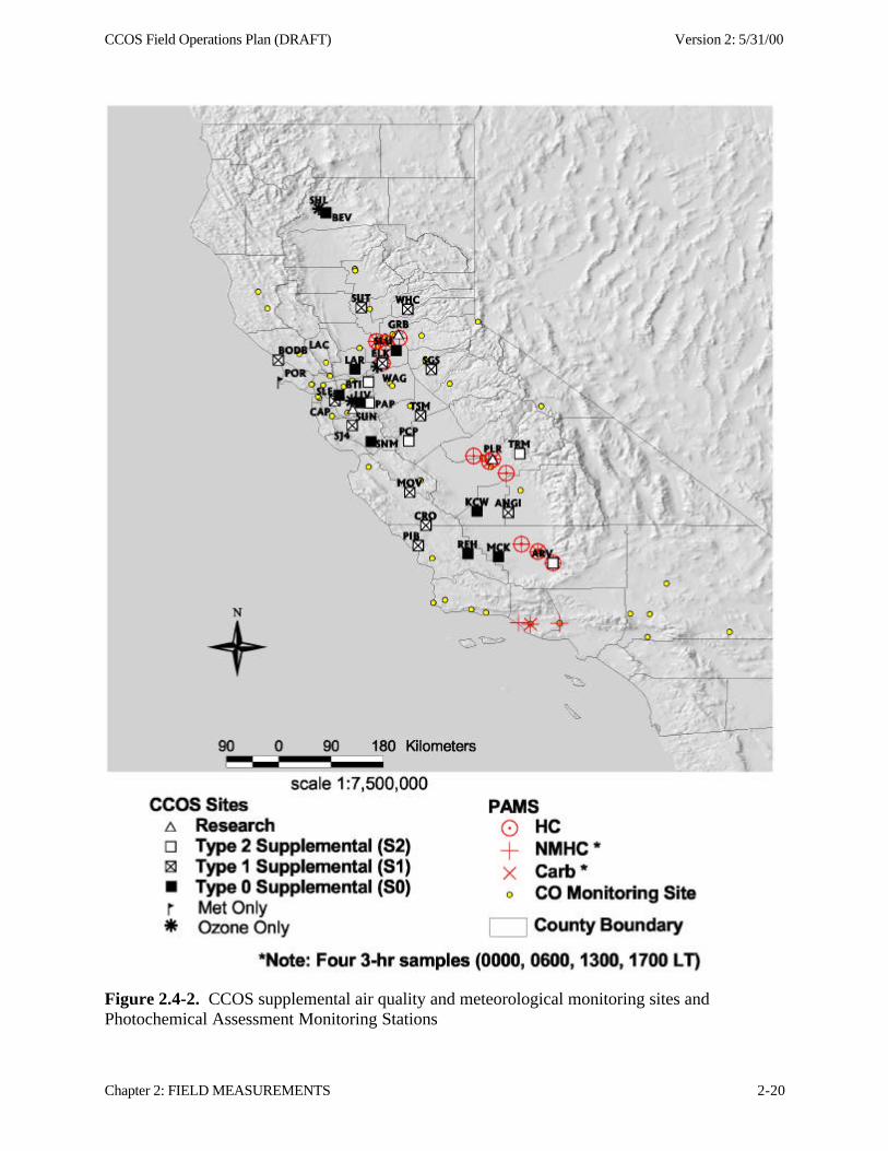
CCOS Field Operations Plan (DRAFT) Version 2: 5/31/00
Chapter 2: FIELD MEASUREMENTS 2-20
Figure 2.4-2. CCOS supplemental air quality and meteorological monitoring sites andPhotochemical Assessment Monitoring Stations
CCOS Field Operations Plan (DRAFT) Version 2: 5/31/00
Chapter 2: FIELD MEASUREMENTS 2-21
2. Continuous ozone during study period.
3. Continuous NO and NOy during study period by a TEI 42S high sensitivitychemiluminescence analyzer with external converter near the sample inlet.
4. Four 3-hour (at 0000-0300, 0600-0900, 1300-1600, and 1700-2000, PDT) canistersamples for up to 15 IOP days to CH4, and analysis by flame ionization detection; andC2-C12 hydrocarbons and MTBE by gas chromatography with flame ionizationdetection.
5. Four 3-hour (at 0000-0300, 0600-0900, 1300-1600, and 1700-2000, PDT) DNPHcartridge samples for up to 15 IOP days for C1-C7 carbonyl compounds by HPLCwith UV detection.
With the exception of NOy measurements, S1 sites are equivalent to PhotochemicalAssessment Monitoring Stations (PAMS) sites. Measurements of speciated volatile organiccompounds (VOC) made under CCOS (four 3-hour samples on 15 IOP days) supplement the 11existing PAMS sites in the study area (four in Sacramento, four in Fresno, and three inBakersfield). The ozone episodic samples that will be collected under PAMS will coincide withthe CCOS IOP days. S1 sites are proposed for Bodega Bay and along the south central coastnorth of Morro Bay at Piedras Blancas to obtain background data near the western boundary ofthe CCOS modeling domain. Sutter Buttes and Turlock provide characterization of ambient airtransported into the upper Sacramento Valley and into the northern San Joaquin Valley,respectively, as a function of the nature of the flow bifurcation downwind of the San FranciscoBay Area. Transport issues will be addressed in the Sierra Foothill communities bysupplementing existing measurements at White Cloud (near Grass Valley) and at San Andreas.Type S1 measurements are also proposed for the CRPAQS Anchor site at Angiola. The BayArea AQMD will operate the existing San Jose and San Leandro monitoring sites as S1 sitesduring CCOS.
Type 2 supplemental monitoring sites (S2) are located at the interbasin transport andintrabasin gradient sites, and near the downwind edge of the urban center where ozone formationmay either be VOC or NOx limited depending upon time of day and pattern of pollutanttransport. S2 sites also provide data for initial conditions and operation evaluations and somediagnostic evaluation of model outputs. The following aerometric parameters are measured atType 2 supplemental monitoring sites.
1. Continuous surface wind speed and direction and temperature during study period.
2. Continuous O3 during study period.
3. Continuous NO and NOy during study period by a high sensitivity TEI 42Schemiluminescence analyzer.
4. Continuous NO2 and peroxyacylnitrate (PAcN) during primary study period by gaschromatography with Luminol detector. A second estimate of HNO3 is obtained bythe difference between NOy and the sum of NO, NO2, and PAcN. This second
CCOS Field Operations Plan (DRAFT) Version 2: 5/31/00
Chapter 2: FIELD MEASUREMENTS 2-22
estimate is an upper-limit because NOy also includes other organic nitrates andparticulate ammonium nitrate.
5. Continuous formaldehyde (HCHO) during primary study period by an instrument thatcontinuously measures the fluorescent, dihydrolutidine derivative formed by thereaction of formaldehyde with 1,3-cyclohexanedione and ammonium ion (Dong andDasgupta, 1994; Fan and Dasgupta, 1994).
6. Four 3-hour (at 0000-0300, 0600-0900, 1300-1600, and 1700-2000, PDT) canistersamples for up to 15 IOP days for analysis of CO, CO2, methane by gaschromatography, reduction of CO and CO2 to CH4, and analysis by flame ionizationdetection; and C2-C12 hydrocarbons and MTBE by gas chromatography with flameionization detection.
7. Four 3-hour (at 0000-0300, 0600-0900, 1300-1600, and 1700-2000, PDT) DNPHcartridge samples for up to 15 IOP days for C1-C7 carbonyl compounds by HPLCwith UV detection.
These measurements allow more detailed assessments of VOC- and NOx-limitation byobservation-driven methods during the entire two-month primary study period. S2 sites areproposed along the three main passes connecting the Bay Area and the Central Valley (BethelIsland, Altamont Pass, and Pacheco Pass. S2 measurements are also proposed Trimmer(downwind of Fresno at the Mouth of the Kings River) and downwind of Bakersfield at theexisting PAMS site at Arvin.
Research sites (R) have the same site requirements as S2 sites. The sites are intended tomeasure a representative urban mix of pollutants, and must be carefully selected to minimize thepotential influence of local emission sources. As with S2 sites, research sites are located whereozone formation may either be VOC or NOx limited depending upon time of day and pattern ofpollutant transport. Research site are intended to provide the maximum extent of high-quality,time-resolved chemical and other aerometric data for rigorous diagnostic evaluation of air qualitymodel simulations and emission inventory estimates. Research sites will be established at Parlier(south of Fresno), Granite Bay (downwind of Sacramento) Fresno, and at Sunol (betweenFremont and Livermore). The following aerometric parameters are measured at Researchmonitoring sites.
1. Continuous surface wind speed and direction and temperature during study period;
2. Continuous ozone during study period;
3. Continuous NO/NOx analyzer during study period.
4. Continuous NOy and NOy* (NOy minus HNO3) during study period with TEI42CY.Nitric acid estimated by difference between the signals with and without a NaClimpregnated fiber denuder.
5. Continuous NO2 and PAcN during primary study period by gas chromatography withLuminol detector. A second estimate of HNO3 is obtained by the difference between
CCOS Field Operations Plan (DRAFT) Version 2: 5/31/00
Chapter 2: FIELD MEASUREMENTS 2-23
NOy and the sum of NO, NO2, and PAcN. This second estimate is an upper-limitbecause NOy also includes organic nitrates and particulate ammonium nitrate.
6. Continuous formaldehyde during primary study period by an instrument thatcontinuously measures the fluorescent, dihydrolutidine derivative formed by thereaction of formaldehyde with 1,3-cyclohexanedione and ammonium ion (Dong andDasgupta, 1994; Fan and Dasgupta, 1994).
7. Semi-continuous hourly organic compound speciation data during primary studyperiod by gas chromatography with ion-trap mass spectrometry. VOC speciationincludes C2 to C12 hydrocarbons, carbonyl and halogenated compounds. Collect up to10 sets of canister and DNPH samples for measurement comparisons with GC/MSand continuous HCHO analyzer.
8. Four 3-hour (at 0000-0300, 0600-0900, 1300-1600, and 1700-2000, PDT) Tenaxcartridge samples for up to 15 IOP days for analysis C8-C20 hydrocarbons
9. Continuous CO by TEI 48C and continuos CO2 by TEI 41C during study period.
10. Actinic flux during study period by scanning radiometer. The radiometers will belocated at the Sunol research site. The other two radiometers will be located at the USDepartment of Agriculture’s UVB Radiation Monitoring site in Davis, 30 miles eastof the Granite Bay research site (see justification below), and at White Cloud, a highelevation site.
11. Semi-continuous particulate nitrate during primary study period by AerosolDynamics Inc. (ADI) automated particle nitrate monitor. The monitor uses anintegrated collection and vaporization cell whereby particles are collected by ahumidified impaction process, and analyzed in place by flash vaporization withquantitation of the evolved gases by chemiluminescent analyzer.
12. Continuos total light absorption by aethalometer and total light scattering by ambientintegrating nephelometer during primary study period.
13. Continuous NO2, HNO3, HCHO and H2O2 on twenty IOP days by dual tunable diodelaser absorption spectrometers at the Parlier research site.
2.4.2 Complementary Measurement Programs
Because a Photochemical Assessment Monitoring Station (PAMS) network does not existin the Bay Area, the density of air quality measurements (e.g., NO/NOy and VOC) in the BayArea is lower than is needed to reliably understand and simulate the conditions that result in daysexceeding the ozone standard in the Bay Area alone. The Bay Area AQMD is sponsoringadditional measurements during CCOS to obtain the information needed to develop a Bay Areaspecific plan. The supplemental Bay Area measurements are primarily designed to increase theunderstanding of high ozone in the Livermore Valley, where the Bay Area’s highest ozone levelsand most frequent exceedances of the standards occur. For this purpose, four types of
CCOS Field Operations Plan (DRAFT) Version 2: 5/31/00
Chapter 2: FIELD MEASUREMENTS 2-24
measurements are proposed: 1) Monitoring of pollutant levels aloft on selected episode days withinstrumented aircraft flights within and upwind of the Livermore Valley; 2) surface monitoringof ozone and precursor gases in the gaps through which air enters and exits the LivermoreValley; and 3) continuous aloft measurements of wind and temperature, using Doppler acousticsounders and radar profilers, above the Livermore Valley and its entrance and exit gaps. TheBAAQMD has contracted T&B Systems to implement the Bay Area component of CCOS. T&BSystem’s effort involves the following tasks.
• Install and operate, from 6/15/00 to 9/15/00, ozone and NOy analyzers at the BAAQMD’sLake Chabot meteorological monitoring site.
• Install and operate, from 6/15/00 to 9/15/00, SODAR, surface meteorology and ozone at asite yet to be determined in the Dublin Canyon.
• Install and operate, from 6/15/00 to 9/15/00, ozone and NOy analyzers at the CCOSLivermore Valley radar profiler site (assuming that this site will be located in theundeveloped area between Livermore and Pleasanton and south of the Livermore airport).These instruments would be collocated with the Elight Ozone Profiler andradiosonde/ozonesonde measurements by the U.S. Navy.
• Install and operate, from 6/15/00 to 9/15/00, an ozone analyzer at the BAAQMD’s KregorPeak meteorological monitoring site.
• Install and operate, from 6/15/00 to 9/15/00, a SODAR with surface meteorology at a site yetto be determined in the San Ramon Valley.
• Install and operate, from 6/15/00 to 9/15/00, a SODAR at the CCOS Sunol research site.
• Assist District staff with installation and operation of mobile sampling equipment (possiblyincluding ozone, NOx, VOC canister sampler, surface met.) on up to 15 IOP days.Measurements will be taken along the 580 corridor through Dublin Canyon and east pastAltamont Pass.
The CCOS field measurement program will be conducted in conjunction with theCalifornia Regional PM10/PM2.5 Air Quality Study (CRPAQS). The CRPAQS includes airquality and meteorological field measurements, emissions characterization, data analysis and airquality modeling. The CRPAQS field study will consist of a long-term campaign from 12/1/99through 1/31/01, a winter intensive study within the period of 11/15/00 through 1/31/01, and afall intensive study within the period of 9/1/00 through 10/31/00. Several experiments will beconducted during the summer period of 7/1/00 through 8/31/00. These include chemicalcharacterization of PM2.5 at the Fresno site to estimate the fraction of fine particles that isattributable to secondary organic aerosol and source contributions of directly-emitted fineparticles. Other experiments will examine the timing and intensity of light extinction in the SanJoaquin Valley and the Mohave Desert. The baseline measurements for CRPAQS, which willbegin in December 1999 and continue to the end of the study, are incorporated and leveragedinto the CCOS field program. These include six upper-air meteorological measurement siteswithin the CCOS domain. Opportunities for cost sharing also exist for purchases of instruments
CCOS Field Operations Plan (DRAFT) Version 2: 5/31/00
Chapter 2: FIELD MEASUREMENTS 2-25
that are needed for both CCOS and the CRPAQS winter intensive study (e.g., NO2, PAN, andNOy and continuous particulate nitrate). CCOS will also benefit from measurements that areavailable throughout the study region from existing federal, state, local, and private air qualityand meteorological monitoring programs.
2.4.3 Equipment Procurement and Checkout
DRI and CE-CERT will develop the specifications of the equipment that are to bepurchased. DRI will be responsible for the ozone analyzers, carbon monoxide analyzers, carbondioxide analyzers, calibration systems, data loggers (at S0, S1, and S2 sites), and diode arrayspectrometers for actinic flux measurements. CE-CERT will be responsible for the NO/NOxanalyzers, NO/NOy and NOy/NOy*3 analyzers and the continuous formaldehyde (HCHO)analyzers. CE-CERT will also be responsible for the continuous nitrogen dioxide (NO2) andperoxyacylnitrate (PacN) analyzers under a separate contract. A version of the computer-baseddata acquisition system (DAS) currently deployed in CRPAQS will be used at the three CCOSresearch sites. Additional CRPAQS DAS that are needed for the winter 2000/2001 study will beprocured by Sonoma Technology, Inc. prior to the summer 2000 so that they may be used at thethree CCOS Research sites. Use of CRPAQS DAS in CCOS will require that CRPAQSparticipants specify the components earlier than would have been necessary for the winterCRPAQS but should not require additional funding. The particulate nitrate analyzers will bepurchased as part of CRPAQS and will be specified according to CRPAQS requirements.Availability of commercial units are assumed. The Aethalometers and nephelometers will also bepurchased as part of CRPAQS and will be specified according to CRPAQS requirements.
DRI will acceptance test the ozone analyzers, carbon monoxide analyzers, carbon dioxideanalyzers, Aethalometers, nephelometers, calibration systems, data loggers (at S0, S1, and S2sites), and diode array spectrometers for actinic flux measurements. The ozone analyzers will bechallenged with ozone generated by DRI’s primary ozone standard, a Dasibi 1008 PC, which isannually compared to the long-path photometer maintained by ARB in Sacramento. The dataacquisition systems will be tested for data collection (serial and analog), calibrator control, andtelephone access. The flow controllers of the calibration systems will be compared to DRI’sNIST-traceable flow meters. The ozone generators of the calibration systems will be calibratedwith DRI’s ozone standard and tested for stability. The particulate nitrate analyzers will betested with NO generated with DRI calibration systems and gases. Nephelometers will be checkwith particle-free air and HFC-134a gas for scattering coefficient. The operations of theAethalometers will be checked. DRI will also test the CRPAQS data acquisition system andadapt the current data collection method to the CCOS instruments.
CE-CERT will acceptance test the NO/NOx analyzers, NO/NOy analyzers, theNOy/NOy* analyzers, the NO2/PacN analyzers (under a separate contract), the HCHO analyzers.The responses of the analyzers to known concentrations of the measured gases will be tested.The NO/NOy and NOy/NOy* analyzers will also be exposed to nitric acid and n-propylnitrate(NPN) to the measurement system and converters.
3 NOy* = NOy minus HNO3
CCOS Field Operations Plan (DRAFT) Version 2: 5/31/00
Chapter 2: FIELD MEASUREMENTS 2-26
Aerosol Dynamics (AD) will acceptance test the particulate nitrate analyzers under anexisting contract for CRPAQS. AD will also assist DRI with the installation and initialcalibration of instrument at the Sunol research site.
2.4.4 Facilities Installation
ENSR will be responsible for site preparation for the Central California Ozone Study.Four sites will be newly established for CCOS (McKittrick, Kettleman City, Piedras Blancas,Granite Bay, Altamont, Lambie Road, Bella Vista). In addition, several existing sites will bemodified as necessary to accommodate CCOS measurements (Bethel Island, Bodega Bay,Pacheco Pass, Trimmer, and Sunol).
ENSR will make final arrangements with landowners to use their land for CCOS, andestablish a written lease agreement. Establish written lease agreements or land use agreements,as necessary. Security fencing and trailer will be installed and electrical and phone service willbe arranged. They will oversee the installation of facilities at each site, and travel to sites, asnecessary, to direct the operations of contractors and to ensure that all facilities are placedproperly.
2.4.5 Equipment Installation and Calibrations
Installation will be performed by DRI and CE-CERT and will be coordinated between thetwo groups so as to be at common sites at overlapping times. This will allow the placement ofthe instrumentation to be made for mutual advantage. It should also allow those site operatorsthat will require training to effectively plan their schedules to limit the amount of time needed fortraining.
DRI will install the O3 analyzers, CO analyzers, CO2 analyzers, calibration systems, dataloggers (at S0, S1, and S2 sites), CRPAQS DAS (at research sites), diode array spectrometers foractinic flux measurements, particulate nitrate analyzers, Aethalometers, and nephelometers. Fullonsite calibrations will be performed on the O3, NO/NOx, CO, CO2 analyzers, particulate nitrateanalyzers and the nephelometers. The diode array spectrometers will be calibrated in Renobefore installation and onsite with a field lamp. Data loggers will be installed, instrumentsconnected, and data collection confirmed at the site and at DRI’s central computer in Reno. Thedata connections will also include those instruments that CE-CERT will install. Any connectionsof existing site instruments to the data loggers will be made. At those existing sites where a sitecalibrator is expected to supply NO and NO2 (Bruceville, Turlock, Bethel Island, and Arvin),those connections will be made such that the current site operations are not adversely affected.The site operators will be trained in the operations of the supplemental instruments. Eachmeasurement will have a standard operating procedure that lists the specific tasks required of thesite operator. They will also contain information on procedure for handling problems andpersonnel to contact for assistance.
CE-CERT will install the NO/NOx analyzers, NO/NOy, NOy/NOy*, and HCHOanalyzers at S2 and R sites as part of this contract and the NO2/PacN analyzers. Full calibrationswill be done for each analyzer. This will include NO, NO2, nitric acid, and n-propyl nitrate(NPN) for the NO/NOy and NOy/NOy* analyzers, HCHO for the HCHO analyzers, and NO2
CCOS Field Operations Plan (DRAFT) Version 2: 5/31/00
Chapter 2: FIELD MEASUREMENTS 2-27
and tridecane for the NO2/PAcN analyzers. Each analyzer will be calibrated at zero and at up tofive upscale points, except tridecane which will only be at one level. Each measurement willhave a standard operating procedure that lists the specific tasks required of the site operator.They will also contain information on procedure for handling problems and personnel to contactfor assistance. DRI will install NO/NOy analyzers at S0 and S1 sites.
T&B will be responsible for operating the Bodega Bay (S1), Turlock (S1), and PechecoPass (S2) sites. Personnel will be present during installation of equipment and will be availablefor training. Training for the Pecheco Pass site will also include training for the gas analyzers.
UCB will be responsible for operating the Sunol (R) and Altamont (S2) sites. Personnelwill be present during installation of equipment and will be available for training. These twosites are heavily equipped but have several instruments in common.
The VOC canister samplers will be installed by Biospheric Research Corporation andDesert Research Institute for the sites indicated in Table 2.4-3. AtmAA will install carbonylcartridge samplers at all CCOS supplemental sites. The site operators will need to be presentduring installation to provide assistance and to insure that the samplers are installed properly anddo not adversely affect the current operations. Training of the site operators on sampleroperations will be done at the time of installation.
DRI will perform final calibrations of the O3 analyzers, CO analyzers, CO2 analyzers,calibration systems, data loggers (at S0, S1, and S2 sites), CRPAQS DAS (at research sites),diode array spectrometers for actinic flux measurements, particulate nitrate analyzers,Aethalometers, and nephelometers. Full onsite calibrations will be performed on the O3,NO/NOx, CO, CO2 analyzers, particulate nitrate analyzers and the nephelometers. The diodearray spectrometers will be calibrated onsite with a field lamp and in Reno after the study. Theflow meters and ozone generators of the calibration systems will be checked after return to Reno.
CE-CERT will perform final calibrations of the NO/NOx analyzers, NO/NOy,NOy/NOy*, HCHO, and the NO2/PacN analyzers analyzers at S2 and R sites. Full calibrationswill be done for each analyzer. This will include NO, NO2, nitric acid, and NPN for the NO/NOyand NOy/NOy analyzers; HCHO for the HCHO analyzers, and NO2 and tridecane for theNO2/PAcN analyzers. Each analyzer will be calibrated at zero and at up to five upscale points,except tridecane which will only be at one level.
T&B will assist in the final calibrations and instrument removal at the Bodega Bay (S1),Turlock (S1), and Pecheco Pass (S2) sites. UCB will assist in the final calibrations andinstrument removal at the Sunol (R) and Altamont (S2) sites. VOC canister samplers and thecarbonyl cartridge samplers will be removed by the respective contractors.
2.4.6 Site Operations
CCOS supplemental analyzers will be calibrated daily using automated calibrationsystems. Details of the calibration methods and standards that will be used are summarized inTable 2.4-4. Automatic calibration checks will be made daily for the O3, NO/NOX, NO/NOY,
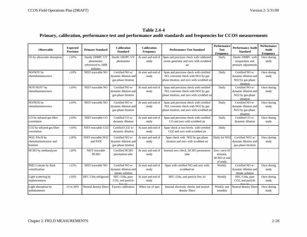
CCOS Field Operations Plan (DRAFT) Version 2: 5/31/00
Chapter 2: FIELD MEASUREMENTS 2-28
Table 2.4-4Primary, calibration, performance test and performance audit standards and frequencies for CCOS measurements
Observable Expected Precision
Primary StandardCalibration Standard
Calibration Frequency
Performance Test StandardPerformance
Test Frequency
Performance Audit Standard
Performance Audit
FrequencyO3 by ultraviolet absorption ±10% Dasibi 1008PC UV
photometer, referenced to ARB
primary
Dasibi 1003PC UV photometer
At start and end of study
Span and precision check with calibrated ozone generator and zero with scrubbed
air
Daily Dasibi 1008PC with temperature and
pressure adjustments
Once during study
NO/NOY by chemiluminescence
±10% NIST-traceable NO Certified NO w/ dynamic dilution and
gas-phase titration
At start and end of study
Span and precision check with certified NO, converter check with NO2 by gas
phase titration, and zero with scrubbed air
Daily Certified NO w/ dynamic dilution and
NO2 by gas-phase titration
Once during study
NOY/NOY* by chemiluminescence
±10% NIST-traceable NO Certified NO w/ dynamic dilution and
gas-phase titration
At start and end of study
Span and precision check with certified NO, converter check with NO2 by gas
phase titration, and zero with scrubbed air
Daily Certified NO w/ dynamic dilution and
NO2 by gas-phase titration
Once during study
NO/NOX by chemiluminescence
±10% NIST-traceable NO Certified NO w/ dynamic dilution and
gas-phase titration
At start and end of study
Span and precision check with certified NO, converter check with NO2 by gas
phase titration, and zero with scrubbed air
Daily Certified NO w/ dynamic dilution and
NO2 by gas-phase titration
Once during study
CO by infrared gas filter correlation
±10% NIST-traceable CO Certified CO w/ dynamic dilution
At start and end of study
Span and precision check with certified CO and zero with scrubbed air
Daily Certified CO w/ dynamic dilution
Once during study
CO2 by infrared gas filter correlation
±10% NIST-traceable CO2 Certified CO2 w/ dynamic dilution
At start and end of study
Span check at two levels with certified CO2 and zero with scrubbed air
Daily - -
NO2, PAcN by chemiluminescence and luminol
±20% NIST-traceable NO2 and PAN
Certified NO w/ dynamic dilution and
gas-phase titration
At start and end of study
Span check with NO2 by gas phase titration and zero with scrubbed air
Daily for NO2 Certified NO2 w/ dynamic dilution and
gas-phase titration
Once during study
HCHO by methanalyzer ±20% NIST-traceable HCHO
Certified HCHO permeation tube
At start and end of study
Internal zero check, HCHO permeation tube
Zero: once/10 minutes,
HCHO at end of study
- -
PM2.5 nitrate by flash volatilization
±15% NIST-traceable NO Certified NO w/ dynamic dilution and
nitrate solution
At start and end of study
Span with certified NO and zero with scrubbed air
Weekly Certified NO w/ dynamic dilution and
nitrate solution
Once during study
Light scattering by nephelometers
±10% HFC-134a refrigerant HFC-134a, pure CO2, and particle
free air
At start and end of study
HFC-134a, and particle free air Weekly HFC-134a, pure CO2, and particle
free air
Once during study
Light absorption by aethalometers
±5 to 20% Neutral density filters Factory calibration When out of spec Internal electronic checks and neutral density filters
Weekly and monthly
Neutral density filters Once during study
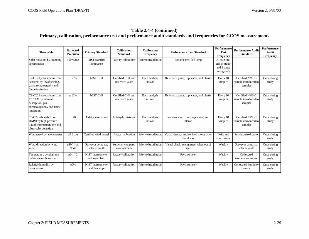
CCOS Field Operations Plan (DRAFT) Version 2: 5/31/00
Chapter 2: FIELD MEASUREMENTS 2-29
Table 2.4-4 (continued)Primary, calibration, performance test and performance audit standards and frequencies for CCOS measurements
Observable Expected Precision
Primary StandardCalibration Standard
Calibration Frequency
Performance Test StandardPerformance
Test Frequency
Performance Audit Standard
Performance Audit
FrequencySolar radiation by scanning spectrometer
±20 w/m2 NIST standard luminance
Factory calibration Prior to installation Portable certified lamp At start and end of study and 3 times during study
- -
C2-C12 hydrocarbons from canisters by cryofocusing, gas chromatography and flame ionization
± 10% NIST CH4 Certified CH4 and reference gases
Each analysis session
Reference gases, replicates, and blanks Every 10 samples
Certified NMHC sample introduced to
sampler
Once during study
C8-C20 hydrocarbons from TENAX by thermal desorption, gas chromatography and flame ionization
± 10% NIST CH4 Certified CH4 and reference gases
Each analysis session
Reference gases, replicates, and blanks Every 10 samples
Certified NMHC sample introduced to
sampler
Once during study
C8-C7 carbonyls from DNPH by high pressure liquid chromatography and ultraviolet detection
± 20 Aldehyde mixtures Aldehyde mixtures Each analysis session
Reference mixtures, replicates, and blanks
Every 10 samples
Certified NMHC sample introduced to
sampler
Once during study
Wind speed by anemometer ±0.3 m/s Certified wind tunnel Factor calibration Prior to installation Visual check, synchronized motor when out of spec
Daily and when needed
Synchronized motor Once during study
Wind direction by wind vane
±10° from North
Surveyor compass, solar azimuth
Surveyor compass, solar azimuth
Prior to installation Visual check, realignment when out of spec
Weekly Surveyor compass, solar azimuth
Once during study
Temperature by platinum resistance or thermister
±0.1 °C NIST thermometer and water bath
Factory calibration Prior to installation Psychrometer Weekly Collocated temperature sensor
Once during study
Relative humidity by capacitance
±2% NIST thermometer and dew cups
Factory calibration Prior to installation Psychrometer Weekly Collocated humidity sensor
Once during study
CCOS Field Operations Plan (DRAFT) Version 2: 5/31/00
Chapter 2: FIELD MEASUREMENTS 2-30
NOY/NOY* analyzers. Each O3 analyzer that is installed as part of CCOS will be challengedwith zero air followed by with ozone concentrations near 400 ppb and 90 ppb to cover the spanand precison levels, respectively. Each NO/NOX, NO/NOY, and NOY/NOY* will bechallenged with zero air followed by NO concentrations near 400 ppb and 90 ppb to cover thespan and precision levels, respectively. A mixture of NO at 30 ppb and NO2 at 60 ppb will begenerated by gas phase titration to check the converter efficiency of the NO/NOX, NO/NOY,and NOY/NOY* analyzers. Data from calibration checks will be retrieved and reviewed daily.
The CCOS supplemental surface air quality and meteorological measurement sites willbe operated by personnel from Desert Research Institute, T&B Systems, University of CaliforniaBerkeley, California Air Resources Board, Bay Area AQMD, Sacramento Metropolitan APCD,San Joaquin Valley Unified APCD, San Luis Obispo County APCD or the Shasta CountyAPCD. Table 2.4-5 provides a summary of the tasks required of local site operators at each typeof supplemental site (S0, S1, S2 or R).
DRI will be responsible for operating the White Cloud (S1) and Granite Bay (R) sites. DRIpersonnel will make weekly visits to the Granite Bay Research site to perform maintenance tasksand to do a visual check of the instruments. Personnel will operate the VOC canisters andcarbonyl cartridges during IOP’s. They will install canisters and cartridges the day before theIOP starts, change canisters and cartridges each day, and remove the final samples at the end ofthe IOP. They will send the filled canisters and exposed cartridges to the proper parties at theexpense of separate contracts. They will also perform minor repairs at the direction of the projectmanager or designee.
T&B will be responsible for operating the Bodega Bay (S1), Turlock (S1), and PechecoPass (S2) sites. Personnel will make weekly visits to the Pecheco Pass site to performmaintenance tasks (e.g., fill reagent reservoirs for NO2/PAN and HCHO analyzers) and to do avisual check of the instruments. Personnel will operate the VOC canisters and carbonylcartridges during IOP’s. They will install canisters and cartridges the day before the IOP starts,change canisters and cartridges each day, and remove the final samples at the end of the IOP.They will send the filled canisters and exposed cartridges to the proper parties at the expense ofseparate contracts. Personnel will also be available for emergency site visits to investigateproblems found during data review. They will also perform minor repairs at the direction of theproject manager or designee.
UCB will be responsible for operating the Sunol (R) and Altamont (S2) sites. Personnelwill make weekly visits to both sites to perform maintenance tasks (e.g., fill reagent reservoirsfor NO2/PAN and HCHO analyzers) and to do a visual check of the instruments. Personnel willoperate the VOC canisters and carbonyl cartridges during IOP’s. They will install canisters andcartridges the day before the IOP starts, change canisters and cartridges each day, and removethe final samples at the end of the IOP. They will send the filled canisters and exposedcartridges to the proper parties at the expense of separate contracts. Personnel will also beavailable for emergency site visits to investigate problems found during data review. They willalso perform minor repairs at the direction of the project manager or designee.
Personnel from the California Air Resources Board and local districts (BAAQMD,SJVAPCD, Shasta County APCD, SLOAPCD) will provide operational support for the other
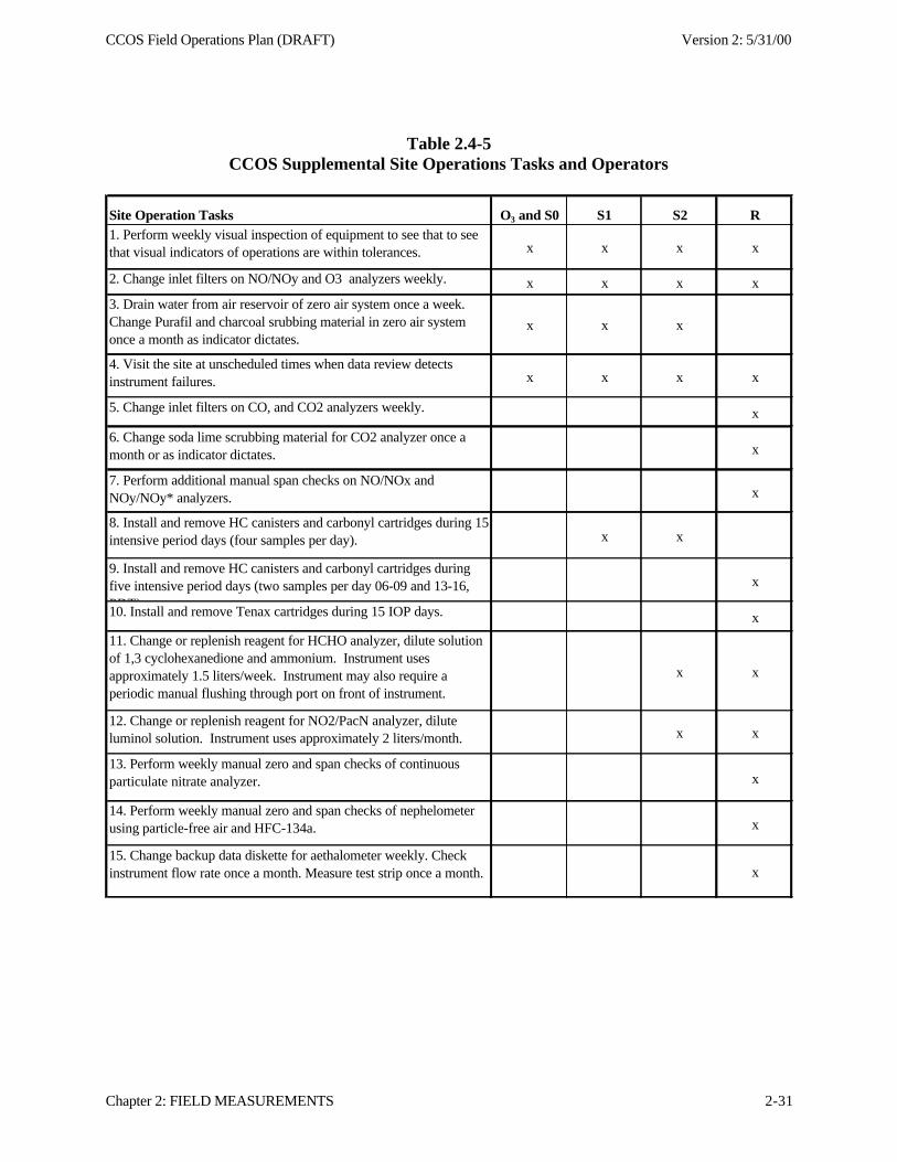
CCOS Field Operations Plan (DRAFT) Version 2: 5/31/00
Chapter 2: FIELD MEASUREMENTS 2-31
Table 2.4-5CCOS Supplemental Site Operations Tasks and Operators
Site Operation Tasks O3 and S0 S1 S2 R1. Perform weekly visual inspection of equipment to see that to see that visual indicators of operations are within tolerances. x x x x
2. Change inlet filters on NO/NOy and O3 analyzers weekly. x x x x
3. Drain water from air reservoir of zero air system once a week. Change Purafil and charcoal srubbing material in zero air system once a month as indicator dictates.
x x x
4. Visit the site at unscheduled times when data review detects instrument failures. x x x x
5. Change inlet filters on CO, and CO2 analyzers weekly. x
6. Change soda lime scrubbing material for CO2 analyzer once a month or as indicator dictates. x
7. Perform additional manual span checks on NO/NOx and NOy/NOy* analyzers. x
8. Install and remove HC canisters and carbonyl cartridges during 15 intensive period days (four samples per day). x x
9. Install and remove HC canisters and carbonyl cartridges during five intensive period days (two samples per day 06-09 and 13-16, PDT)
x
10. Install and remove Tenax cartridges during 15 IOP days. x
11. Change or replenish reagent for HCHO analyzer, dilute solution of 1,3 cyclohexanedione and ammonium. Instrument uses approximately 1.5 liters/week. Instrument may also require a periodic manual flushing through port on front of instrument.
x x
12. Change or replenish reagent for NO2/PacN analyzer, dilute luminol solution. Instrument uses approximately 2 liters/month. x x
13. Perform weekly manual zero and span checks of continuous particulate nitrate analyzer. x
14. Perform weekly manual zero and span checks of nephelometer using particle-free air and HFC-134a. x
15. Change backup data diskette for aethalometer weekly. Check instrument flow rate once a month. Measure test strip once a month. x
CCOS Field Operations Plan (DRAFT) Version 2: 5/31/00
Chapter 2: FIELD MEASUREMENTS 2-32
CCOS supplemental surface air quality sites that are not mentioned above. Details of the agencysupport are specified in Appendix D1.
DRI will transfer all continuous CCOS supplemental surface data (except meteorologicaldata) and District ozone data from the CCOS sites to a central computer in Reno every day.Ozone data from other sites of interest for forecast will be provided by the ARB. These data willautomatically be summarized and will be reviewed daily to track instrument performance. Inparticular, the calibration checks will be tracked on control charts. Any problems that ariseduring data review will be investigated. Local site personnel will be informed of the problemsand solutions will be devised, either onsite or through an emergency site visit.
DRI will be available to provide technical assistance on the O3, CO, CO2 analyzers,calibration systems, data loggers (at S0, S1, and S2 sites), CRPAQS DAS (at research sites),diode array spectrometers for actinic flux measurements, particulate nitrate analyzers,Aethalometers, and nephelometers. The assistance will probably be through telephone or e-mail.Personnel will also be available for emergency site visits to investigate problems, found duringdata review, which cannot be resolved by on-site operators. DRI will be responsible for servicecalls (for all supplemental equipment) for all CCOS sites that are located north of theMerced/Madera county line.
CE-CERT will be available to provide technical assistance to DRI personnel and to siteoperators on the operations of the NO/NOx, NO/NOy, NOy/NOy*, HCHO, and NO2/PacNanalyzers. The assistance will probably be through telephone or e-mail. A catastrophic failureof one of these instruments may require a site visit by CE-CERT or DRI or the return of theinstrument to CE-CERT. CE-CERT will also review summary data from the NO/NOy,NOy/NOy*,HCHO, and NO2/PacN instruments for an additional check of their operations. CE-CERT will be responsible for service calls (for all supplemental equipment) for all CCOS sitesthat are located south of the Merced/Madera county line
2.4.7 Maintenance and Repair
Personnel will be available at DRI and CE-CERT for technical support during the CCOSfield study for both routine operations and for problems as they arise. Field personnel will beable to communicate with technical support personnel through telephone and/or e-mail at anytime. Field personnel will be notified as to the responsible support person for the variousmeasurements. Support personnel will be designated to be available for non-working hoursperiods, particularly during IOP days.
The technical support personnel will also be available for consultation with thoseperforming the daily data reviews. If a problem is found, technical support personnel will benotified. They will in turn determine how best to fix the problem, weighing both speed and costof the solution. In most cases, the fastest and least expensive solution will involve directing thestation operator to fix the problem. For major problems, such as an analyzer failure, it will benecessary for technical support personnel to visit the site and either repair onsite or arrange forreplacement equipment.
CCOS Field Operations Plan (DRAFT) Version 2: 5/31/00
Chapter 2: FIELD MEASUREMENTS 2-33
2.4.8 Data Acquisition and Review
In general, data acquisition at existing sites consists of an onsite data logger to collect andaverage data, which are automatically transferred to a central computer through a telephonemodem. The transfers can be as often as once an hour. Each time the site is polled, new data areappended to the data file for that site.
CCOS supplemental data will be obtained in a similar manner through data loggers thatwill be installed at the sites. A central CCOS computer located at DRI in Reno will beconfigured to call the sites once a day to obtain supplementary CCOS data. The calling timeswill be set so as not to interfere with site operations. In addition, the district data will beuploaded as well. Collection and screening of the district data will ensure the highest level ofdata completeness and will provide a complete picture of what is happening at all CCOS sites innear real time. These data also will be useful in supplementing forecast information.
Since there are over five different agencies involved in data collection, the manner inwhich the data are obtained may vary. Obtaining the data within 24 hours of collection will be apriority. One method will be to call the district data logger during a designated window andobtain the data directly. Another method is for the agency to transfer their data to an accessiblefile transfer protocol (FTP) computer daily and then the CCOS computer downloads data fromthe FTP site(s).
Due to the variability in formats of the district data, this portion of the data acquisitionsystem will require the greatest amount of preparation. Information will need to be gathered foreach site on: acquisition software, download windows, telephone numbers or FTP addresses anddirectories, parameters collected (name, order, units, averaging times, time stamps, delimiters,etc.), and calibration periods and target values.
Each morning new data collected by the central CCOS computer will be evaluated.Several electronic reports will be generated during the evaluation and will be available to theCCOS team on an area of the DRI network dedicated to the CCOS project. Each step in theevaluation will be automated to the extent possible. These screening checks are designed tocatch a failure in a measurement system, which in turn triggers prompt corrective action to avoidlarge data losses.
The first step in the evaluation will be to verify that all sites were polled successfully. Asimple error report will be generated that lists any sites where a connection was not made. Next,a running table will be updated that lists the start and stop times of the data collected with anygaps noted. Once the evaluation of data completeness is performed, simple statistics will becalculated (e.g. mean, max, min, etc.) and archived. The values will be scanned for outliers andif any are noted an error report will be generated.
Where feasible, rates of change and inter-parameter relationship checks will be calculated(e.g. temperature values that change too rapidly during a two hour period, relationship betweenozone and NOY). The emphasis of rates of change checks will be applied with caution. Criteriaused for rates of change are often difficult to set properly due to the variability of conditions atsites located in a large geographical region. If the criteria are set too narrow, unnecessary error
CCOS Field Operations Plan (DRAFT) Version 2: 5/31/00
Chapter 2: FIELD MEASUREMENTS 2-34
reports are generated resulting in wasted time investigating natural phenomena. If set too wide,real instrument malfunctions can be missed. Special summary reports tailored for forecasters willbe generated each morning and made available to CCOS management.
Where applicable, calibration data will be extracted from the downloaded data. The datawill be screened and evaluated for frequency and target values. A running calibration file will bearchived and an error report will be generated if the frequency and found values do not meetrequirements of target values. Each morning any error report(s) generated will be reviewed andthe problem triggering the report will be investigated. This investigation may include manuallypolling the site to review the real time data and/or plotting the data (time series, interparameterplots, site comparison plots, etc.). If a potential or immediate problem is confirmed, thePrinciple Investigator and the site operator will be notified.
Following screening runs, non-CCOS supplementary data will be archived into weeklyfiles and saved as backup data until project completion. CCOS data files will be concatenatedinto monthly files for data validation.
Data files will be constructed using specifications and formats described in:
Appendix C- Data Management of the CCOS Field Study Plan
(http://www.arb.ca.gov/ccaqs/ccos/ccosmtgsdocs_v3w.htm) .
Averaged data will be re-timed to have a start hour time stamp (i.e. 0100 would representan average that starts at 0100 and ends at 0105 for 5 minute averages or 0159 for hourlyaverages). All times will be Pacific Standard Time. Calibration/audit data will be set to missingin the validated database, as will any known invalid data.
Data screening is applied to level 0 data. Monthly level 0 files will be processed tovalidation Level 1B and merged with validated district data for each CCOS site. The cause of allmissing values will be documented and flagged. Continuous data will be reviewed using timeseries plots. The graphs quickly reveal any data anomalies due to power failures or instrumentmalfunction. Copies of field logs will be obtained and reviewed. Significant events will bechecked against the graphs and data reports for consistency.
Calibration data will be reviewed to assess the precision of the data. If the calibrationsindicate invalid or low precision, data values will be deleted or re-scaled as necessary andappropriate flags will be applied. Only obvious invalid data will be deleted. Suspect data will bereported but flagged as suspect. Once data have been processed to this point, the outlier and rateof change checks applied to level 0 data will be reapplied to the processed data to ensure that noanomalous data remain. The areal distribution of select parameters will be reviewed for theentire network to check for values that appear spatially anomalous.
Final validated district data will be obtained and merged with the final supplementaryCCOS data to form one database for submittal to the CCOS data manager. The format of the filewill follow the conventions specified in Section 5. The final data base will include all continuouscollected at the surface sites during CCOS except the meteorological data. The database willcontain hourly averaged data from all measurements as well as data averaged over shorter
CCOS Field Operations Plan (DRAFT) Version 2: 5/31/00
Chapter 2: FIELD MEASUREMENTS 2-35
periods, probably five-minute averages. The one-hour database is dictated by the practice of thedistrcts to report hourly data. The supplemental CCOS data will be also collected and reported atthe shorter averaging time. Integrated data, such as from the VOC canister collection and thecarbonyl cartridge collection will be reported separately.
2.5 CCOS Ground-Based Aloft Air Quality and Meteorological Measurements
Meteorological soundings will be used to obtain information on temperature, relativehumidity, and wind at various levels of the atmosphere above ground level. Radiosondes releasesduring IOPs will provide in situ measurements of pressure, temperature, humidity, and windspeed and direction at various altitudes above ground. These balloons will also carry anozonsonde that will provide a vertical profile of ozone. Two types of remote sounding, radarwind profilers and Doppler acoustic sounders, will provide continuous measurements of upper-air winds during the entire four-month CCOS measurement period (6/1/00 to 9/30/00). Table2.5-1 provides a summary of the aloft meteorological measurements that are currently beingmade by local agencies and that will be made by during CCOS by the EnvironmentalTechnology Laboratory (ETL, Boulder, CO) and Air Resources Laboratory (ARL, Idaho Falls,ID) of the National Oceanic and Atmospheric Administration (NOAA), Sonoma Technology,Inc. (STI), and T&B systems. Figures 2.5-1 and 2.5-2 show the locations of the upper-airmeteorological measurement sites.
2.5.1 Continuous Upper-Air Meteorological Measurements
Radar Wind Profilers (RWP) provide sequential horizontal and vertical wind componentsin data assimilation and model comparison on a sub-hour time scale. RWPs generally acquiremeasurements within 100 to 150 m thick layers between ~0.150 and 3 km AGL with a minimumvertical resolution of 60 meters. A radio-acoustic sounding system (RASS) are used to quantifyvirtual temperature to elevations of ~1 km AGL (up to 2 km AGL in ideal conditions), but this isinsufficient altitude to characterize the daytime mixed layers of 2–3 km AGL often observed inmuch of the study area. Acoustic Sounders (Sodars), like RWPs, also acquire continuousmeasurements of winds aloft. Sodars have better vertical resolution (~30 m layers from ~50 to600 m AGL) but less vertical range (750 m AGL maximum). Sodars are most applicable inlocations with lower-level structure, such as that found in marine layers, in channeling throughcanyons and passes, and in nighttime radiation inversions.
Radar profilers, doppler sodars, and RASS are used at most sites because they acquirehourly average wind speed, wind direction, and temperature by remote sensing without constantoperator intervention. Sodars are collocated with profilers at several locations because theyprovide greater vertical resolution in the first 100 m agl. Several radar profilers are beinginstalled to acquire a multi-year database, and one of the important functions of theCCOS/CRPAQS supplements to this network is to relate these relatively sparse measurementstothe detailed meteorological patterns determined during CCOS. The ARB operates twoprofilers (with RASS) in the San Joaquin Valley, and the San Joaquin Unified APCD andSacramento Metropolitan AQMD operate one profiler/RASS each as part of their PAMSmonitoring program. Military facilities with operational profilers include Travis AFB,Vandenberg AFB, and the Naval Post Graduate School in Monterey. Because these profilers are
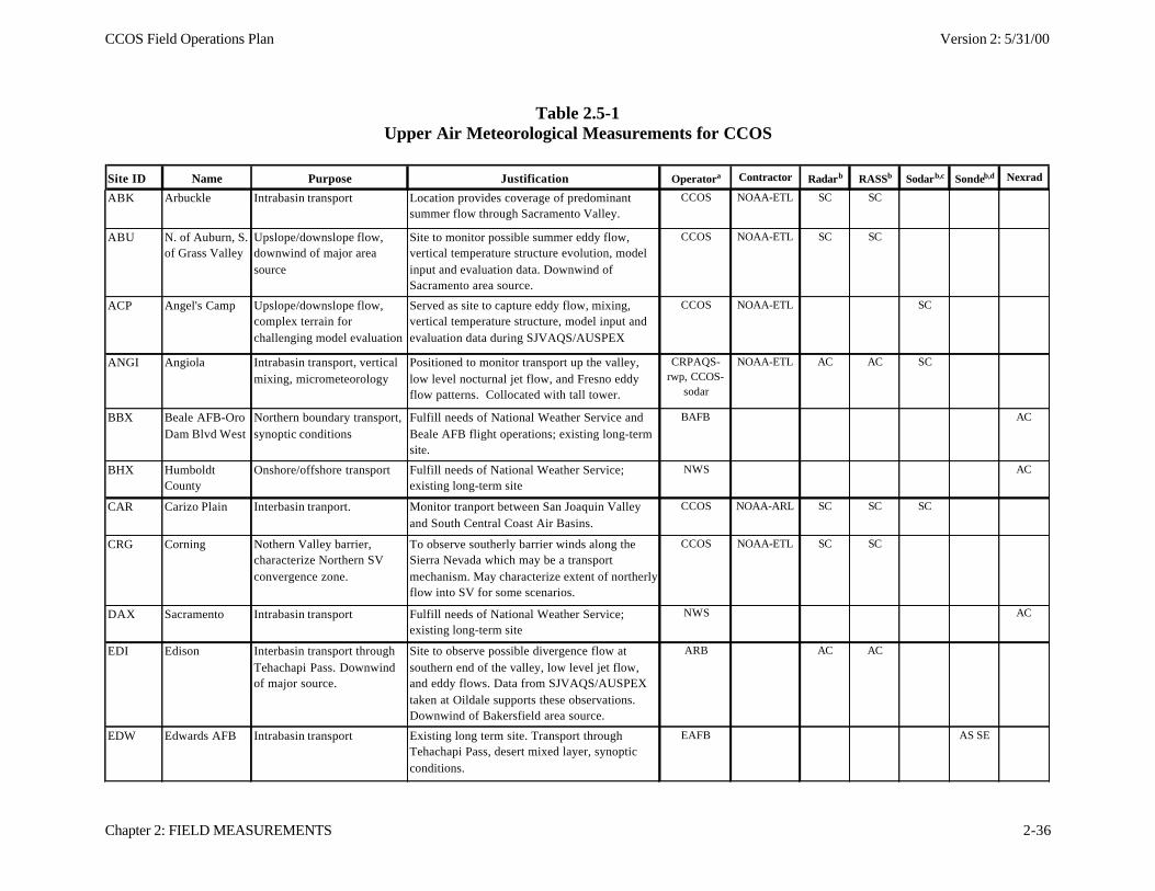
CCOS Field Operations Plan Version 2: 5/31/00
Chapter 2: FIELD MEASUREMENTS 2-36
Table 2.5-1Upper Air Meteorological Measurements for CCOS
Site ID Name Purpose Justification Operatora Contractor Radarb RASSb Sodarb,c Sondeb,d Nexrad
ABK Arbuckle Intrabasin transport Location provides coverage of predominant summer flow through Sacramento Valley.
CCOS NOAA-ETL SC SC
ABU N. of Auburn, S. of Grass Valley
Upslope/downslope flow, downwind of major area source
Site to monitor possible summer eddy flow, vertical temperature structure evolution, model input and evaluation data. Downwind of Sacramento area source.
CCOS NOAA-ETL SC SC
ACP Angel's Camp Upslope/downslope flow, complex terrain for challenging model evaluation
Served as site to capture eddy flow, mixing, vertical temperature structure, model input and evaluation data during SJVAQS/AUSPEX
CCOS NOAA-ETL SC
ANGI Angiola Intrabasin transport, vertical mixing, micrometeorology
Positioned to monitor transport up the valley, low level nocturnal jet flow, and Fresno eddy flow patterns. Collocated with tall tower.
CRPAQS-rwp, CCOS-
sodar
NOAA-ETL AC AC SC
BBX Beale AFB-Oro Dam Blvd West
Northern boundary transport, synoptic conditions
Fulfill needs of National Weather Service and Beale AFB flight operations; existing long-term site.
BAFB AC
BHX Humboldt County
Onshore/offshore transport Fulfill needs of National Weather Service; existing long-term site
NWS AC
CAR Carizo Plain Interbasin tranport. Monitor tranport between San Joaquin Valley and South Central Coast Air Basins.
CCOS NOAA-ARL SC SC SC
CRG Corning Nothern Valley barrier, characterize Northern SV convergence zone.
To observe southerly barrier winds along the Sierra Nevada which may be a transport mechanism. May characterize extent of northerly flow into SV for some scenarios.
CCOS NOAA-ETL SC SC
DAX Sacramento Intrabasin transport Fulfill needs of National Weather Service; existing long-term site
NWS AC
EDI Edison Interbasin transport through Tehachapi Pass. Downwind of major source.
Site to observe possible divergence flow at southern end of the valley, low level jet flow, and eddy flows. Data from SJVAQS/AUSPEX taken at Oildale supports these observations. Downwind of Bakersfield area source.
ARB AC AC
EDW Edwards AFB Intrabasin transport Existing long term site. Transport through Tehachapi Pass, desert mixed layer, synoptic conditions.
EAFB AS SE
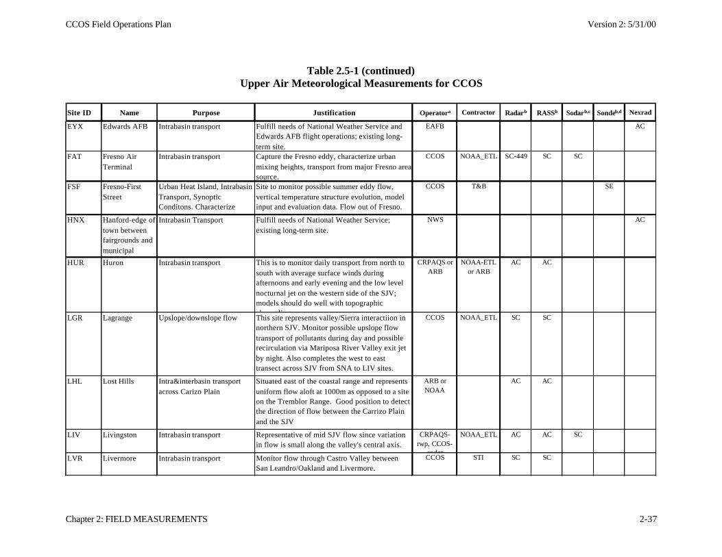
CCOS Field Operations Plan Version 2: 5/31/00
Chapter 2: FIELD MEASUREMENTS 2-37
Table 2.5-1 (continued)Upper Air Meteorological Measurements for CCOS
Site ID Name Purpose Justification Operatora Contractor Radarb RASSb Sodarb,c Sondeb,d Nexrad
EYX Edwards AFB Intrabasin transport Fulfill needs of National Weather Service and Edwards AFB flight operations; existing long-term site.
EAFB AC
FAT Fresno Air Terminal
Intrabasin transport Capture the Fresno eddy, characterize urban mixing heights, transport from major Fresno area source.
CCOS NOAA_ETL SC-449 SC SC
FSF Fresno-First Street
Urban Heat Island, Intrabasin Transport, Synoptic Conditons. Characterize winds at major area source.
Site to monitor possible summer eddy flow, vertical temperature structure evolution, model input and evaluation data. Flow out of Fresno.
CCOS T&B SE
HNX Hanford-edge of town between fairgrounds and municipal airport
Intrabasin Transport Fulfill needs of National Weather Service; existing long-term site.
NWS AC
HUR Huron Intrabasin transport This is to monitor daily transport from north to south with average surface winds during afternoons and early evening and the low level nocturnal jet on the western side of the SJV; models should do well with topographic channeling.
CRPAQS or ARB
NOAA-ETL or ARB
AC AC
LGR Lagrange Upslope/downslope flow This site represents valley/Sierra interactiion in northern SJV. Monitor possible upslope flow transport of pollutants during day and possible recirculation via Mariposa River Valley exit jet by night. Also completes the west to east transect across SJV from SNA to LIV sites.
CCOS NOAA_ETL SC SC
LHL Lost Hills Intra&interbasin transport across Carizo Plain
Situated east of the coastal range and represents uniform flow aloft at 1000m as opposed to a site on the Tremblor Range. Good position to detect the direction of flow between the Carrizo Plain and the SJV
ARB or NOAA
AC AC
LIV Livingston Intrabasin transport Representative of mid SJV flow since variation in flow is small along the valley's central axis.
CRPAQS-rwp, CCOS-
sodar
NOAA_ETL AC AC SC
LVR Livermore Intrabasin transport Monitor flow through Castro Valley between San Leandro/Oakland and Livermore.
CCOS STI SC SC
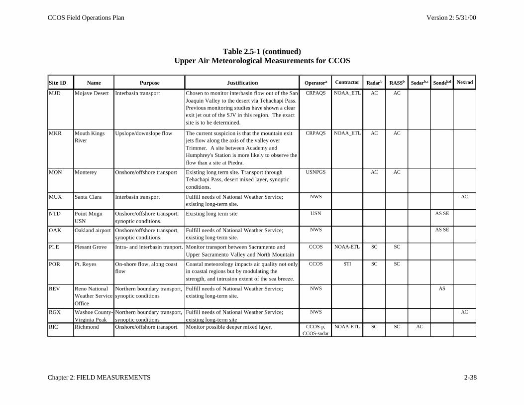
CCOS Field Operations Plan Version 2: 5/31/00
Chapter 2: FIELD MEASUREMENTS 2-38
Table 2.5-1 (continued)Upper Air Meteorological Measurements for CCOS
Site ID Name Purpose Justification Operatora Contractor Radarb RASSb Sodarb,c Sondeb,d Nexrad
MJD Mojave Desert Interbasin transport Chosen to monitor interbasin flow out of the San Joaquin Valley to the desert via Tehachapi Pass. Previous monitoring studies have shown a clear exit jet out of the SJV in this region. The exact site is to be determined.
CRPAQS NOAA_ETL AC AC
MKR Mouth Kings River
Upslope/downslope flow The current suspicion is that the mountain exit jets flow along the axis of the valley over Trimmer. A site between Academy and Humphrey's Station is more likely to observe the flow than a site at Piedra.
CRPAQS NOAA_ETL AC AC
MON Monterey Onshore/offshore transport Existing long term site. Transport through Tehachapi Pass, desert mixed layer, synoptic conditions.
USNPGS AC AC
MUX Santa Clara Interbasin transport Fulfill needs of National Weather Service; existing long-term site.
NWS AC
NTD Point Mugu USN
Onshore/offshore transport, synoptic conditions.
Existing long term site USN AS SE
OAK Oakland airport Onshore/offshore transport, synoptic conditions.
Fulfill needs of National Weather Service; existing long-term site.
NWS AS SE
PLE Plesant Grove Intra- and interbasin tranport. Monitor transport between Sacramento and Upper Sacramento Valley and North Mountain Counties.
CCOS NOAA-ETL SC SC
POR Pt. Reyes On-shore flow, along coast flow
Coastal meteorology impacts air quality not only in coastal regions but by modulating the strength, and intrusion extent of the sea breeze.
CCOS STI SC SC
REV Reno National Weather Service Office
Northern boundary transport, synoptic conditions
Fulfill needs of National Weather Service; existing long-term site.
NWS AS
RGX Washoe County-Virginia Peak
Northern boundary transport, synoptic conditions
Fulfill needs of National Weather Service; existing long-term site
NWS AC
RIC Richmond Onshore/offshore transport. Monitor possible deeper mixed layer. CCOS-p, CCOS-sodar
NOAA-ETL SC SC AC
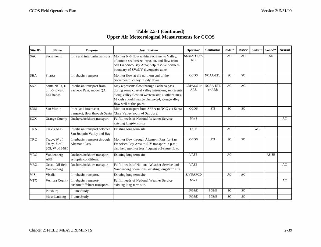
CCOS Field Operations Plan Version 2: 5/31/00
Chapter 2: FIELD MEASUREMENTS 2-39
Table 2.5-1 (continued)Upper Air Meteorological Measurements for CCOS
Site ID Name Purpose Justification Operatora Contractor Radarb RASSb Sodarb,c Sondeb,d Nexrad
SAC Sacramento Intra and interbasin transport Monitor N-S flow within Sacramento Valley, afternoon sea breeze intrusion, and flow from San Francisco Bay Area; help resolve northern boundary of SV/SJV divergence zone.
SMUAPCD/ARB
AC AC SE
SHA Shasta Intrabasin transport Monitor flow at the northern end of the Sacramento Valley. Eddy flows.
CCOS NOAA-ETL SC SC
SNA Santa Nella, E of I-5 toward Los Banos
Interbasin transport from Pacheco Pass, model QA.
May represents flow through Pacheco pass during some coastal valley intrusions; represents along-valley flow on western side at other times. Models should handle channeled, along-valley flow well at this point.
CRPAQS or ARB
NOAA-ETL or ARB
AC AC
SNM San Martin Intra- and interbasin transport, flow through Santa Clara Valley.
Monitor transport from SFBA to NCC via Santa Clara Valley south of San Jose.
CCOS STI SC SC
SOX Orange County Onshore/offshore transport. Fulfill needs of National Weather Service; existing long-term site
NWS AC
TRA Travis AFB Interbasin transport between San Joaquin Valley and Bay Area.
Existing long term site TAFB AC WC
TRC Tracy, W of Tracy, S of I-205, W of I-580
Interbasin transport through Altamont Pass.
Monitor flow through Altamont Pass for San Francisco Bay Area to SJV transport in p.m.; also help monitor less frequent off-shore flow.
CCOS STI SC SC
VBG Vandenberg AFB
Onshore/offshore transport, synoptic conditions.
Existing long term site VAFB AC AS SE
VBX Orcutt Oil field-Vandenberg AFB
Onshore/offshore transport. Fulfill needs of National Weather Service and Vandenberg operations; existing long-term site.
VAFB AC
VIS Visalia Intrabasin transport. Existing long term site SJVUAPCD AC AC
VTX Ventura County Intrabasin transport-onshore/offshore transport.
Fulfill needs of National Weather Service; existing long-term site.
NWS AC
Pittsburg Plume Study PG&E PG&E SC SC
Moss Landing Plume Study PG&E PG&E SC SC
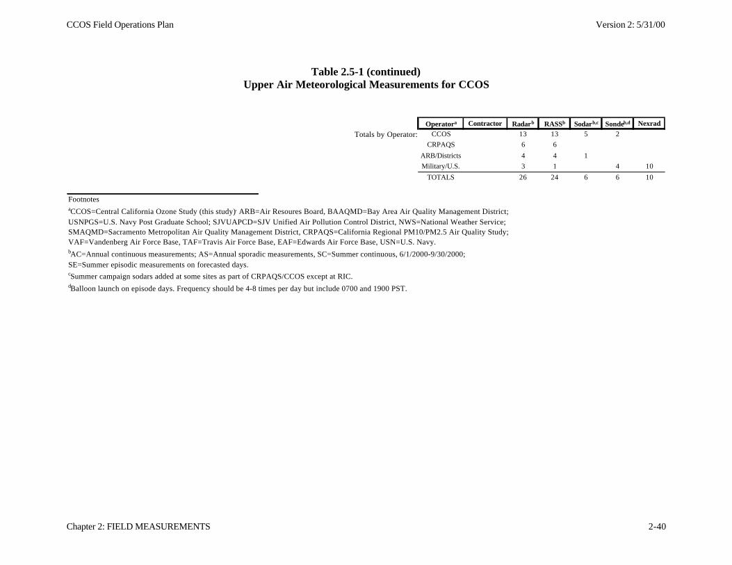
CCOS Field Operations Plan Version 2: 5/31/00
Chapter 2: FIELD MEASUREMENTS 2-40
Table 2.5-1 (continued)Upper Air Meteorological Measurements for CCOS
Operatora Contractor Radarb RASSb Sodarb,c Sondeb,d Nexrad
Totals by Operator: CCOS 13 13 5 2
CRPAQS 6 6
ARB/Districts 4 4 1
Military/U.S. 3 1 4 10
TOTALS 26 24 6 6 10
FootnotesaCCOS=Central California Ozone Study (this study), ARB=Air Resoures Board, BAAQMD=Bay Area Air Quality Management District;USNPGS=U.S. Navy Post Graduate School; SJVUAPCD=SJV Unified Air Pollution Control District, NWS=National Weather Service;SMAQMD=Sacramento Metropolitan Air Quality Management District, CRPAQS=California Regional PM10/PM2.5 Air Quality Study;VAF=Vandenberg Air Force Base, TAF=Travis Air Force Base, EAF=Edwards Air Force Base, USN=U.S. Navy.bAC=Annual continuous measurements; AS=Annual sporadic measurements, SC=Summer continuous, 6/1/2000-9/30/2000;SE=Summer episodic measurements on forecasted days.cSummer campaign sodars added at some sites as part of CRPAQS/CCOS except at RIC.dBalloon launch on episode days. Frequency should be 4-8 times per day but include 0700 and 1900 PST.
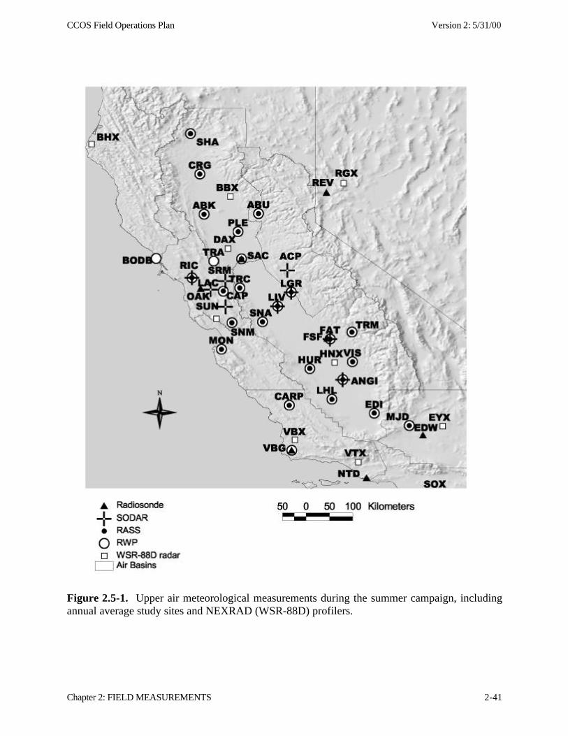
CCOS Field Operations Plan Version 2: 5/31/00
Chapter 2: FIELD MEASUREMENTS 2-41
Figure 2.5-1. Upper air meteorological measurements during the summer campaign, includingannual average study sites and NEXRAD (WSR-88D) profilers.
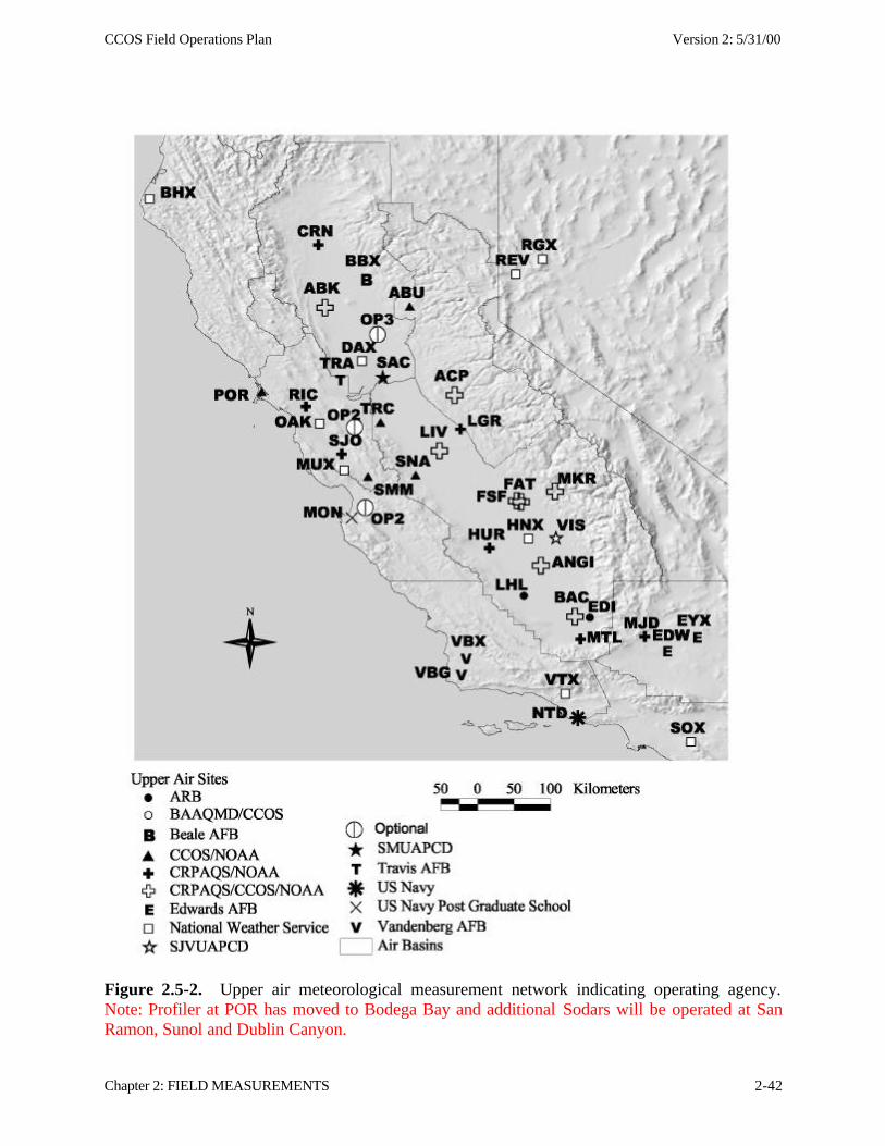
CCOS Field Operations Plan Version 2: 5/31/00
Chapter 2: FIELD MEASUREMENTS 2-42
Figure 2.5-2. Upper air meteorological measurement network indicating operating agency.Note: Profiler at POR has moved to Bodega Bay and additional Sodars will be operated at SanRamon, Sunol and Dublin Canyon.
CCOS Field Operations Plan Version 2: 5/31/00
Chapter 2: FIELD MEASUREMENTS 2-43
operated by different entities, equivalent methods of data evaluation and reporting need to beestablished among these entities prior to CCOS field study. As part of CRPAQS, NOAA willupgrade existing equipment, as required, at these facilities, and coordinate data collection toensure compatibility with the CRPAQS/CCOS upper-air database. Six profiles/RASS will beinstalled and operational during summer 2000 as part of the CRPAQS. In addition, nineprofilers/RASS and 5 sodars will be installed for the CCOS summer 2000 field study.
Another Sodar will be located in the vicinity of the power plant stacks selected for studyto ensure that the local 3D winds are well defined for accurate model simulation during thecrucial early stages of plume dispersion. Measurements are planned for the power plants at MossLanding and at Pittsburgh and the radar/RASS profiler will be moved as necessary.
2.5.2 Radiosondes/Ozonesondes
Radiosondes are needed to determine changes in relative humidity and to quantifyconditions at elevations above ~2000 m agl. They are also the only practical means of acquiringupper air measurements in cities where the noise and siting requirements of remote sensingdevices make them difficult to operate. Radiosondes are routinely launched through the year at0400 and 1600 PST from Oakland, with additional launches at Vandenberg, Edwards, and Pt.Mugu according to military mission requirements. None of these locations are within the CentralValley, so these will be supplemented by launches at Sacramento and in the southern SanJoaquin Valley on 15 episodic days during summer with six radiosondes (with ozonesonde)releases per day. The 490 MHz RWP will be placed in the Fresno area to provide higher verticalsoundings in the central San Joaquin Valley.
T&B Systems staff, assisted by in-kind personnel at the Sacramento site, will take sixozonesondes at one site and four ozonesondes at the other during each of 14 IOP days. On oneIOP day (for a total of 15), six soundings will be performed at both Fresno and Bakersfield sites.Proposed sounding release times on the six/day schedule are 05, 08, 11, 14, 17, and 22 PDT.Proposed sounding release times on the four/day schedule are 05, 11, 14, 17, and 22 PDT. Theschedule will be determined from the forecast episode characteristics. If the episode is expectedhave a greater impact the northern area of the Central Valley, the more frequent schedule will becarried out at Sacramento. Conversely, the frequent schedule will occur at Fresno if impacts areforecast to be greater in the south. On one day, it is anticipated that six soundings will be madeat both sites.
Equipment will be installed and tested prior to commencement of primary study period.Ozonesonde conditioning and testing laboratory will be set up at an existing T&B facility atModesto. Training will be conducted for two site technicians. At the same time, in-kind supportpersonnel will gain experience assisting in balloon launches.
Ozonesonde data will be processed to Level 0 on-site immediately after the completion ofeach flight. The Level 0 data for will be transmitted to the T&B Systems electronic data basearchives via internet after each flight. Initial Level 0 checks for completeness and accuracy willbe conducted as possible after receipt by experienced personnel. Ozonesonde flight data will bevalidated by T&B to Level 1.
CCOS Field Operations Plan Version 2: 5/31/00
Chapter 2: FIELD MEASUREMENTS 2-44
In addition to releases by T&B Systems, the Naval Air Warfare Center at Pt Mugu willrelease several radiosondes with ozonesonde in the Bay Area (Dublin) for comparison with theElight ground-base ozone profiler and northern San Joaquin Valley (Tracy or Stockton) duringCCOS IOPs.
In addition to ozonesondes mentioned in the previous section, aloft air qualitymeasurements are available from fixed platforms that are part of the routine monitoring network(e.g., Walnut Grove radio tower and Sutter Buttes). CCOS will add NOy and speciatedhydrocarbon measurements at Sutter Buttes to provide additional information on oxidantsavailable as carry-over to mix-down on the following day.
2.5.3 Ozone LIDAR
The CCOS Technical Committee discussed the merits of using airborne and ground-based LIDARs to obtain vertical profiles of ozone concentrations, and reached the consensus thata small fleet of instrumented aircraft would provide a more cost-effective approach given thetradeoffs between temporal and spatial information and requirements for pollutant flux andplume measurements. The rationale for the Committee’s recommendation is explained further inSection 4.8 or the CCOS Field Study Plan. Although ozone LIDAR was not included in theCCOS Field Study Plan (Fujita et al., 1999), Elight Laser Systems, a German company, willdeploy their commercial Ozone Profiler during CCOS using in-kind resources. The profiler willbe installed in Dublin and will make measurements for one month beginning in early August,2000.
The Ozone Profiler measure vertical ozone profiles starting at approximately 50 m up to2000 m with a detection limit of 5µg/m³ with 200 m range resolution. The system can bedelivered as outdoor version with air-water cooling and with water-water cooling as indoorversion. The optics and the electronics are integrated in an outdoors housing which allowssystem operation under different weather conditions. In the system a data analysis softwarepackage is implemented for the on-line determination of the ozone concentration as function ofthe height. This information can be delivered in form of ASII files or as graphical tables.Technical specification for the Elight Ozone Profiler is available at their web site athttp://www.elight.de/profiler2.htm.
2.6 In-Situ Aircraft Measurements
Instrumented aircraft will be used to measure the three dimensional distribution of ozone,ozone precursors, and meteorological variables. For CCOS, aircraft data have five specific uses:
• Aloft boundary and initial conditions – direct input to model.
• Definition of temporal and spatial ozone patterns in layers aloft – model evaluation.
• Direct measurement of mixing depth during spirals – model evaluation and manycorroborative studies.
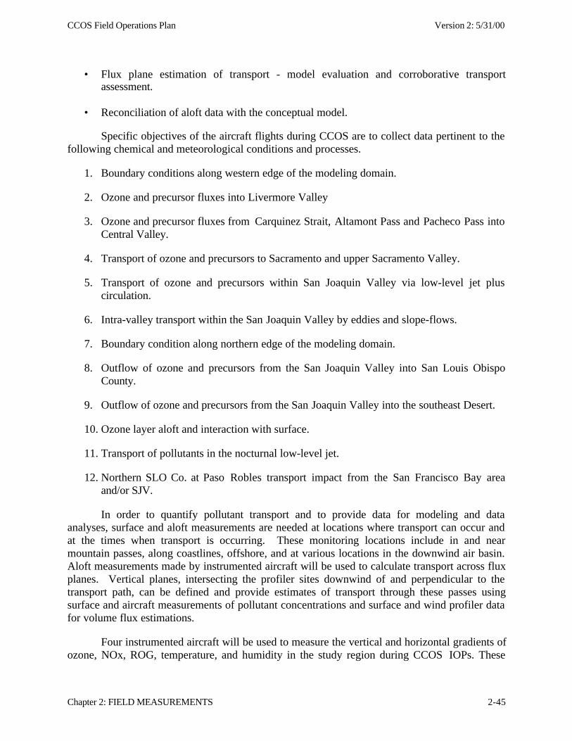
CCOS Field Operations Plan Version 2: 5/31/00
Chapter 2: FIELD MEASUREMENTS 2-45
• Flux plane estimation of transport - model evaluation and corroborative transportassessment.
• Reconciliation of aloft data with the conceptual model.
Specific objectives of the aircraft flights during CCOS are to collect data pertinent to thefollowing chemical and meteorological conditions and processes.
1. Boundary conditions along western edge of the modeling domain.
2. Ozone and precursor fluxes into Livermore Valley
3. Ozone and precursor fluxes from Carquinez Strait, Altamont Pass and Pacheco Pass intoCentral Valley.
4. Transport of ozone and precursors to Sacramento and upper Sacramento Valley.
5. Transport of ozone and precursors within San Joaquin Valley via low-level jet pluscirculation.
6. Intra-valley transport within the San Joaquin Valley by eddies and slope-flows.
7. Boundary condition along northern edge of the modeling domain.
8. Outflow of ozone and precursors from the San Joaquin Valley into San Louis ObispoCounty.
9. Outflow of ozone and precursors from the San Joaquin Valley into the southeast Desert.
10. Ozone layer aloft and interaction with surface.
11. Transport of pollutants in the nocturnal low-level jet.
12. Northern SLO Co. at Paso Robles transport impact from the San Francisco Bay areaand/or SJV.
In order to quantify pollutant transport and to provide data for modeling and dataanalyses, surface and aloft measurements are needed at locations where transport can occur andat the times when transport is occurring. These monitoring locations include in and nearmountain passes, along coastlines, offshore, and at various locations in the downwind air basin.Aloft measurements made by instrumented aircraft will be used to calculate transport across fluxplanes. Vertical planes, intersecting the profiler sites downwind of and perpendicular to thetransport path, can be defined and provide estimates of transport through these passes usingsurface and aircraft measurements of pollutant concentrations and surface and wind profiler datafor volume flux estimations.
Four instrumented aircraft will be used to measure the vertical and horizontal gradients ofozone, NOx, ROG, temperature, and humidity in the study region during CCOS IOPs. These
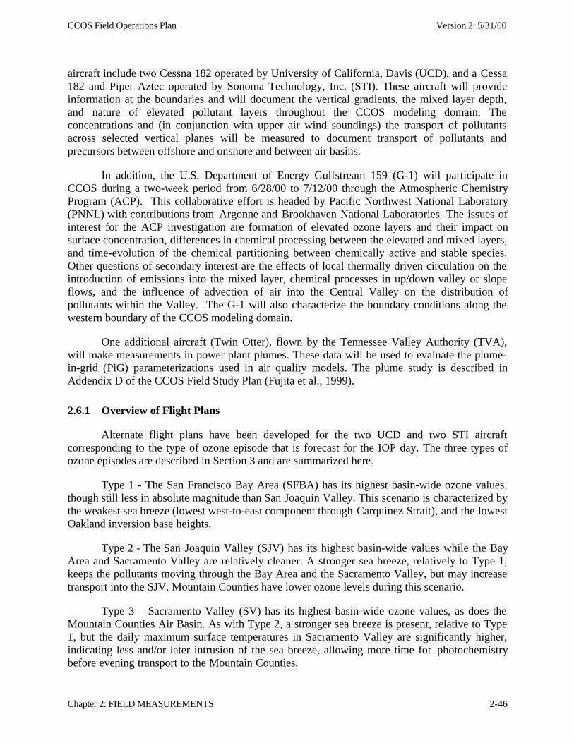
CCOS Field Operations Plan Version 2: 5/31/00
Chapter 2: FIELD MEASUREMENTS 2-46
aircraft include two Cessna 182 operated by University of California, Davis (UCD), and a Cessa182 and Piper Aztec operated by Sonoma Technology, Inc. (STI). These aircraft will provideinformation at the boundaries and will document the vertical gradients, the mixed layer depth,and nature of elevated pollutant layers throughout the CCOS modeling domain. Theconcentrations and (in conjunction with upper air wind soundings) the transport of pollutantsacross selected vertical planes will be measured to document transport of pollutants andprecursors between offshore and onshore and between air basins.
In addition, the U.S. Department of Energy Gulfstream 159 (G-1) will participate inCCOS during a two-week period from 6/28/00 to 7/12/00 through the Atmospheric ChemistryProgram (ACP). This collaborative effort is headed by Pacific Northwest National Laboratory(PNNL) with contributions from Argonne and Brookhaven National Laboratories. The issues ofinterest for the ACP investigation are formation of elevated ozone layers and their impact onsurface concentration, differences in chemical processing between the elevated and mixed layers,and time-evolution of the chemical partitioning between chemically active and stable species.Other questions of secondary interest are the effects of local thermally driven circulation on theintroduction of emissions into the mixed layer, chemical processes in up/down valley or slopeflows, and the influence of advection of air into the Central Valley on the distribution ofpollutants within the Valley. The G-1 will also characterize the boundary conditions along thewestern boundary of the CCOS modeling domain.
One additional aircraft (Twin Otter), flown by the Tennessee Valley Authority (TVA),will make measurements in power plant plumes. These data will be used to evaluate the plume-in-grid (PiG) parameterizations used in air quality models. The plume study is described inAddendix D of the CCOS Field Study Plan (Fujita et al., 1999).
2.6.1 Overview of Flight Plans
Alternate flight plans have been developed for the two UCD and two STI aircraftcorresponding to the type of ozone episode that is forecast for the IOP day. The three types ofozone episodes are described in Section 3 and are summarized here.
Type 1 - The San Francisco Bay Area (SFBA) has its highest basin-wide ozone values,though still less in absolute magnitude than San Joaquin Valley. This scenario is characterized bythe weakest sea breeze (lowest west-to-east component through Carquinez Strait), and the lowestOakland inversion base heights.
Type 2 - The San Joaquin Valley (SJV) has its highest basin-wide values while the BayArea and Sacramento Valley are relatively cleaner. A stronger sea breeze, relatively to Type 1,keeps the pollutants moving through the Bay Area and the Sacramento Valley, but may increasetransport into the SJV. Mountain Counties have lower ozone levels during this scenario.
Type 3 – Sacramento Valley (SV) has its highest basin-wide ozone values, as does theMountain Counties Air Basin. As with Type 2, a stronger sea breeze is present, relative to Type1, but the daily maximum surface temperatures in Sacramento Valley are significantly higher,indicating less and/or later intrusion of the sea breeze, allowing more time for photochemistrybefore evening transport to the Mountain Counties.
CCOS Field Operations Plan Version 2: 5/31/00
Chapter 2: FIELD MEASUREMENTS 2-47
All three types have some degree of stagnation (i.e., reduced SF to Reno pressuregradients) that reduces the effects of the marine intrusion. Types 2 and 3 have stronger marine-air intrusion relative Type 1. SJV experiences greatest stagnation with Type 2, while SV hasgreater stagnation with Type 3. It is easier to distinguish Type 1 from Type 2 and 3 and moredifficult to forecast between Type 2 and Type 3. Therefore, lower confidence is associated withthe Forecast Team’s ability to predict ozone episode in the Redding Area.
Figures 2.6-1, 2.6-2, and 2.6-3 show diagrams of the flight paths for the two UCDCessna, STI Aztec, STI Cessna, and PNNL G-1 (western boundary flights only). One UCDCessna will capture the flow through the Carquinez Strait, through the delta and into the northernSJV, and the flow approaching and leaving Sacramento. The second UCD Cessna will documentthe conditions in the Bay Area in the morning and in locations east of the Berkeley Hills in theafternoon. It will also capture the flow in and around the Livermore Valley and the flow throughAltamont Pass to Tracy. Both UCD aircraft will make several afternoon flights during non-IOPdays to document conditions across and along the Sacramento Valley. The STI Piper Aztec willdocument conditions along the western and northern boundaries and the STI Cessna will coverthe San Joaquin Valley. Boundary measurements will be made during both non-episode andepisode days. When the Aztec is not flying along the boundaries, it will participate in flux planemeasurements. The following sections describe the capabilities and objectives of each of theaircraft and proposed flight plan under different meteorological scenario.
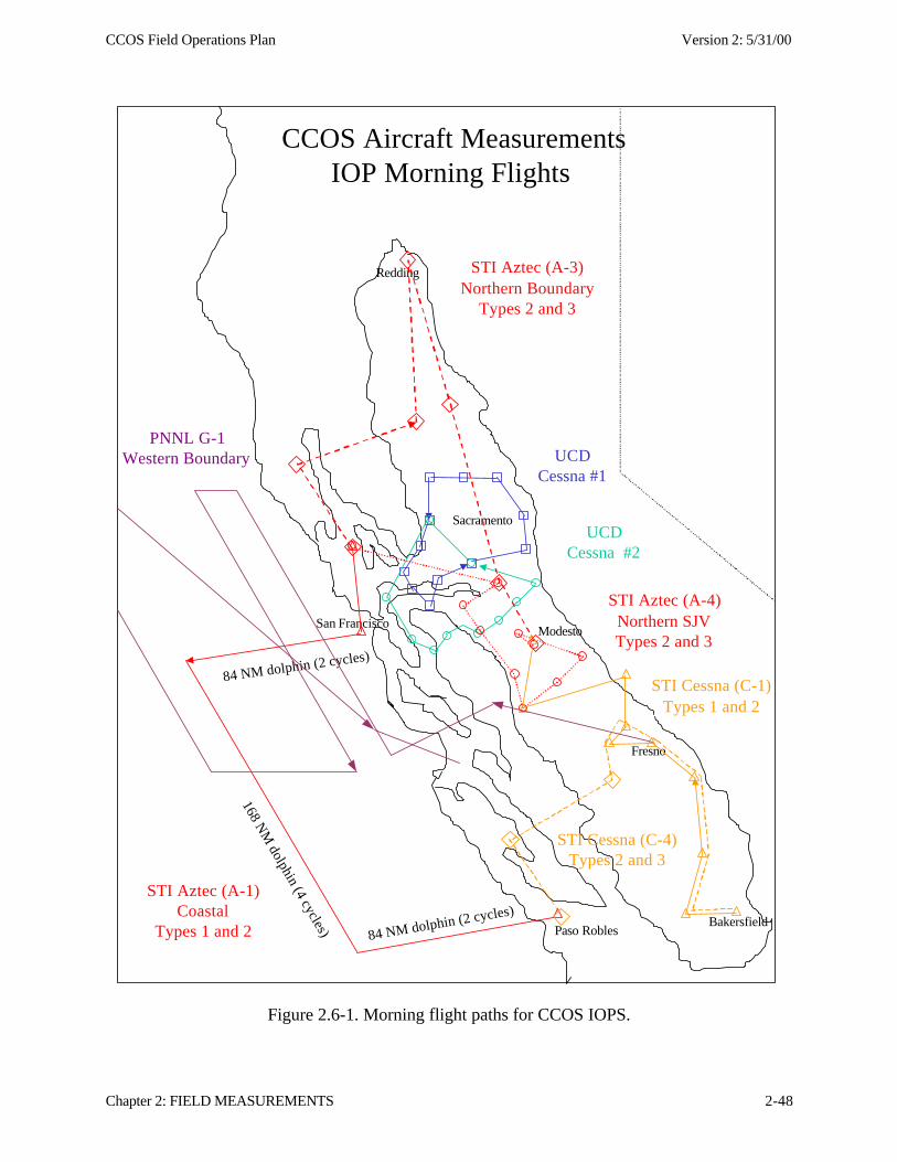
CCOS Field Operations Plan Version 2: 5/31/00
Chapter 2: FIELD MEASUREMENTS 2-48
Sacramento
Fresno
Bakersfield
Redding
San Francisco
UCDCessna #1
UCDCessna #2
CCOS Aircraft MeasurementsIOP Morning Flights
84 NM dolphin (2 cycles)
84 NM dolphin (2 cycles)
168 NM
dolphin (4 cycles)
STI Aztec (A-1)Coastal
Types 1 and 2
STI Aztec (A-3)Northern Boundary
Types 2 and 3
STI Aztec (A-4)Northern SJVTypes 2 and 3
STI Cessna (C-1)Types 1 and 2
Paso Robles
Modesto
STI Cessna (C-4)Types 2 and 3
PNNL G-1Western Boundary
Figure 2.6-1. Morning flight paths for CCOS IOPS.
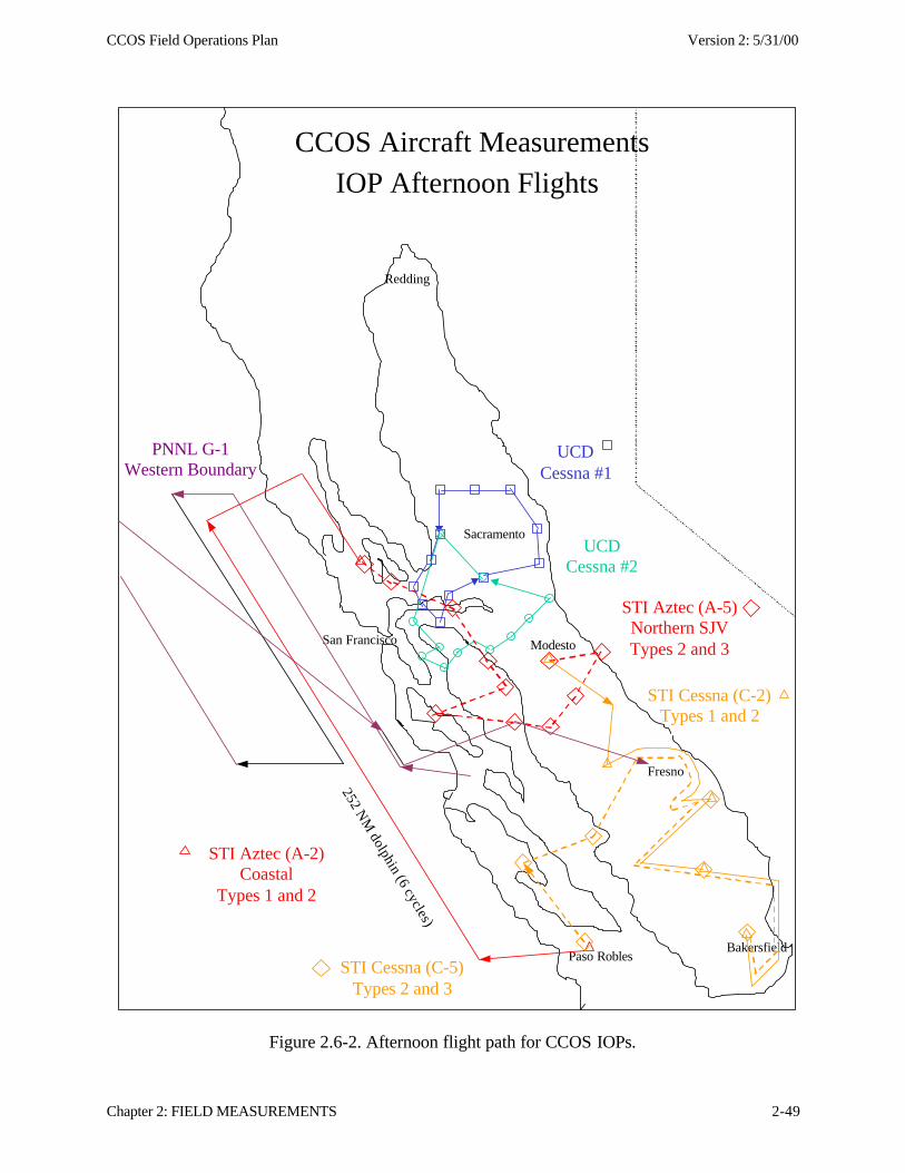
CCOS Field Operations Plan Version 2: 5/31/00
Chapter 2: FIELD MEASUREMENTS 2-49
Sacramento
Fresno
Bakersfield
Redding
San Francisco
CCOS Aircraft Measurements
IOP Afternoon Flights
UCDCessna #1
UCDCessna #2
Paso Robles
Modesto
252 NM
dolphin (6 cycles)
STI Aztec (A-2)Coastal
Types 1 and 2
STI Aztec (A-5)Northern SJVTypes 2 and 3
STI Cessna (C-2)Types 1 and 2
STI Cessna (C-5)Types 2 and 3
PNNL G-1Western Boundary
Figure 2.6-2. Afternoon flight path for CCOS IOPs.
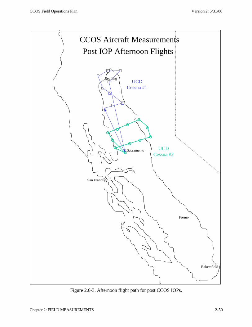
CCOS Field Operations Plan Version 2: 5/31/00
Chapter 2: FIELD MEASUREMENTS 2-50
Sacramento
Fresno
Bakersfield
Redding
San Francisco
CCOS Aircraft Measurements
Post IOP Afternoon Flights
UCDCessna #1
UCDCessna #2
Figure 2.6-3. Afternoon flight path for post CCOS IOPs.
CCOS Field Operations Plan Version 2: 5/31/00
Chapter 2: FIELD MEASUREMENTS 2-51
2.6.2 University of California, Davis Cessna 182 (UCD #1 and UCD #2)
Aircraft: Single engine.
UCD #1 Measurements: Position (Garmin GPS); humidity, temperature, wind speed, and winddirection (Aventech AIMMS-10); O3 (Dasibi 1008); NO, NOy (TEI 42S), particle concentration(Climet); hydrocarbons (3 canisters per flight, 90 total, analyzed by BRC); carbonyl compounds(3 DNPH cartridges from 40 liter Tedlar bags, 90 total, analyzed by AtmAA).UCD #2 Measurements: Position (Garmin GPS); humidity, temperature, wind speed, and winddirection (Aventech AIMMS-10); O3 (Dasibi 1008); NO, NOy (TEI 42S), hydrocarbons (4canisters per flight, 136 total, analyzed by BRC); carbonyl compounds (4 DNPH cartridges fromTedlar bags, 136 total, analyzed by AtmAA).
Hours Contracted: Each aircraft is budgeted for 120 hours during IOPs and additional flights onnon-IOPs.Base Airport: Davis for both aircraft.Area of Coverage: Delta, Sacramento, and downwind of Sacramento include some flights inSacramento Valley.Objectives of flights during IOPs – all catagories:1. Capture the flow through the Carquinez Strait2. Capture the flow through the delta and into the Northern SJV3. Capture flow approaching and leaving Sacramento.4. Define conditions in the bay area in the AM and behind the Berkeley hills in the PM.5. Capture conditions in and around Livermore AM and PM6. Capture flow through Altamont pass and to Tracy7. Have daily camparisions between both aircraft and the Elk Grove RASS (Franklin field)Objectives of flight during non-IOPs Sacramento valley:1. Capture conditions across and along the valley.
Operational Constraints: Standby period from 6/1/00 to 9/15/00.Quality Assurance Audits: Performance audits of O3 and NOy analyzers by ARB qualityassurance section on 6/12/00 and 6/13/00 in Dixon.Data Comparisons: Both UCD aircraft will depart within 5 minutes of each other to afford dailycross-comparisons on climb out. Coordinate parallel flight with STI aircraft and fly by radarwind profilers.Flight Plans: Basic flight patterns to will be spiral climb over Davis followed by vertical sawtooth patterns: ascents along the straight lines shown in the figures and descending spirals(actually squares) at the rectangles shown. Note these boxes are approximately to scale or a littlelarger than the actual expected pattern. Altitude variation to be from (near) the surface to about4500’ AGL. While the aircraft paths sometimes cross or spiral near the same locations these willbe displaced in time by 45 to 75 minutes.
Figure 2.6-1. 2.6-2, and 2.6-3 show the flight path for all IOPS for both aircraft duringmorning IOPs, afternoon IOPs and afternoon on post IOPs, respectively. All flights will require 3to 3.5 hours to complete. Morning flights will depart at 0600, returning by 0930 PDT, andafternoon flights will depart 1300 and return 1630 PDT.
CCOS Field Operations Plan Version 2: 5/31/00
Chapter 2: FIELD MEASUREMENTS 2-52
2.6.3 Sonoma Technology Inc. Piper Aztec
Aircraft: Twin engine
Measurements: Position (Garmin 250); humidity, temperature, wind speed, and wind direction(Aventech AIMMS-10); dew point (Cambridge Systems 137-C); Temperature (YSI/MRI);Temperature backup (Rosemont 102 (O3 (Monitor Labs 8410E); NO, NOy (TEI 42S); bscat(MRI 1560 modified by Waggoner) (particle concentration (Climet); hydrocarbons (4 canistersper flight, 136 total, analyzed by BRC); carbonyl compounds (4 DNPH cartridges from Tedlarbags, 136 total, analyzed by AtmAA). Approximately 2-5 minute VOC samples.
Hours Contracted: 136Base Airport: Santa RosaArea of coverage: Western and Northern BoundariesOperational Constraints: Standby period from 7/2/00 to 9/2/00.Quality Assurance Audits: Performance audits of O3 and NOy analyzers by ARB qualityassurance section on 7/3/00 in Santa Rosa.Data Comparisons: Coordinate parallel flight with UCD aircraft and fly by radar wind profilers.Flight Plans: See Tables 2.6-1 to 2.6-5.
2.6.4 (Sonoma Technology Inc. Cessna 182
Aircraft: Single engine
Measurements: Position (Garmin 250); humidity, temperature, wind speed, and wind direction(Aventech AIMMS-10); dew point (Cambridge Systems 137-C); Temperature (YSI/MRI);Temperature backup (Rosemont 102 (O3 (Monitor Labs 8410E); NO, NOy (TEI 42S); bscat(MRI 1560 modified by Waggoner) (particle concentration (Climet); hydrocarbons (3 canistersper flight, 90 total, analyzed by BRC); carbonyl compounds (3 DNPH cartridges from Tedlarbags, 90 total, analyzed by AtmAA). Approximately 2-5 minute VOC samples.
Hours Contracted: 136Base Airport: BakersfieldArea of coverage: San Joaquin ValleyOperational Constraints: Standby period from 7/2/00 to 9/2/00.Quality Assurance Audits: Performance audits of O3 and NOy analyzers by ARB qualityassurance section in early July.Data Comparisons: Coordinate parallel flight with UCD aircraft and fly by radar wind profilers.Flight Plans: See Table 2.6-6 to 2.6-10.
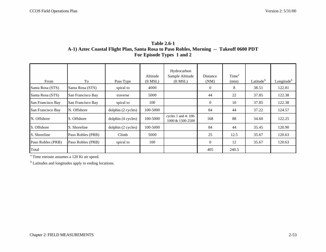
CCOS Field Operations Plan Version 2: 5/31/00
Chapter 2: FIELD MEASUREMENTS 2-53
Table 2.6-1A-1) Aztec Coastal Flight Plan, Santa Rosa to Paso Robles, Morning -- Takeoff 0600 PDT
For Episode Types 1 and 2
From To Pass TypeAltitude (ft MSL)
Hydrocarbon Sample Altitude
(ft MSL)Distance
(NM)Timea
(min) Latitudeb Longitudeb
Santa Rosa (STS) Santa Rosa (STS) spiral to 4000 0 8 38.51 122.81
Santa Rosa (STS) San Francisco Bay traverse 5000 44 22 37.85 122.38
San Francisco Bay San Francisco Bay spiral to 100 0 10 37.85 122.38
San Francisco Bay N. Offshore dolphin (2 cycles) 100-5000 84 44 37.22 124.57
N. Offshore S. Offshore dolphin (4 cycles) 100-5000cycles 1 and 4: 100-1000 & 1500-2500 168 88 34.60 122.25
S. Offshore S. Shoreline dolphin (2 cycles) 100-5000 84 44 35.45 120.90
S. Shoreline Paso Robles (PRB) Climb 5000 25 12.5 35.67 120.63
Paso Robles (PRB) Paso Robles (PRB) spiral to 100 0 12 35.67 120.63
Total 405 240.5
a Time enroute assumes a 120 Kt air speed.b Latitudes and longitudes apply to ending locations.
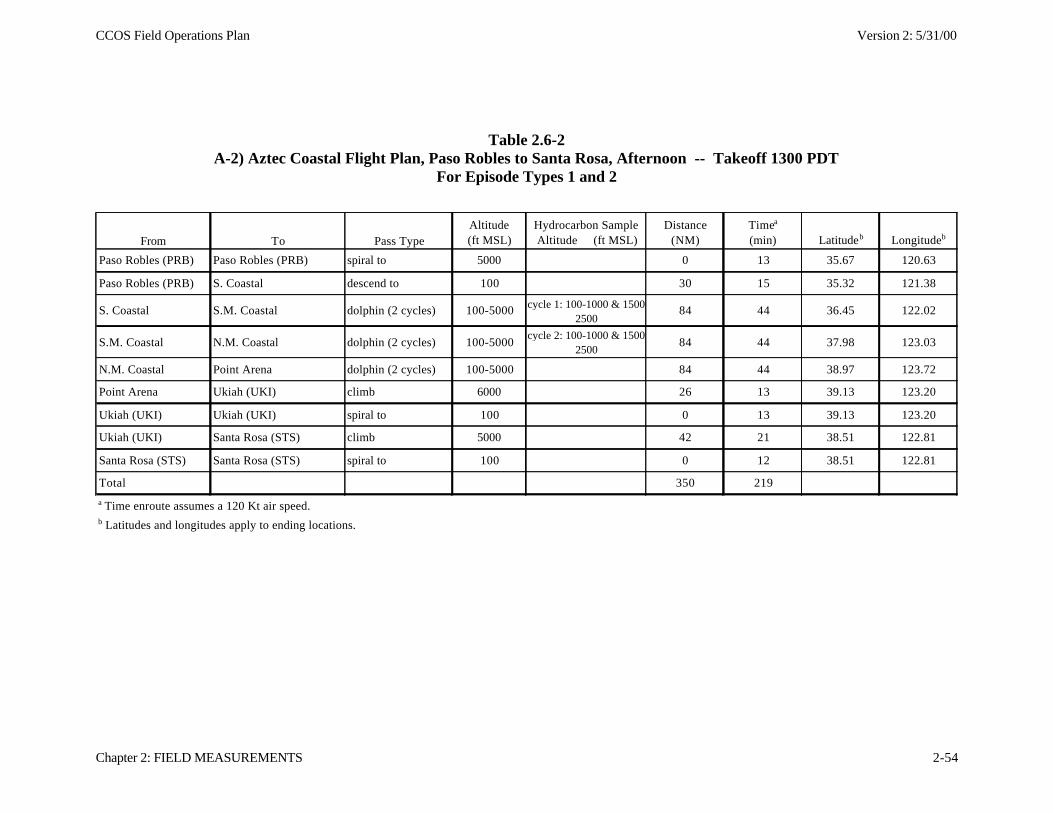
CCOS Field Operations Plan Version 2: 5/31/00
Chapter 2: FIELD MEASUREMENTS 2-54
Table 2.6-2A-2) Aztec Coastal Flight Plan, Paso Robles to Santa Rosa, Afternoon -- Takeoff 1300 PDT
For Episode Types 1 and 2
From To Pass TypeAltitude (ft MSL)
Hydrocarbon Sample Altitude (ft MSL)
Distance (NM)
Timea
(min) Latitudeb Longitudeb
Paso Robles (PRB) Paso Robles (PRB) spiral to 5000 0 13 35.67 120.63
Paso Robles (PRB) S. Coastal descend to 100 30 15 35.32 121.38
S. Coastal S.M. Coastal dolphin (2 cycles) 100-5000 cycle 1: 100-1000 & 1500-2500
84 44 36.45 122.02
S.M. Coastal N.M. Coastal dolphin (2 cycles) 100-5000cycle 2: 100-1000 & 1500-
250084 44 37.98 123.03
N.M. Coastal Point Arena dolphin (2 cycles) 100-5000 84 44 38.97 123.72
Point Arena Ukiah (UKI) climb 6000 26 13 39.13 123.20
Ukiah (UKI) Ukiah (UKI) spiral to 100 0 13 39.13 123.20
Ukiah (UKI) Santa Rosa (STS) climb 5000 42 21 38.51 122.81
Santa Rosa (STS) Santa Rosa (STS) spiral to 100 0 12 38.51 122.81
Total 350 219
a Time enroute assumes a 120 Kt air speed.b Latitudes and longitudes apply to ending locations.
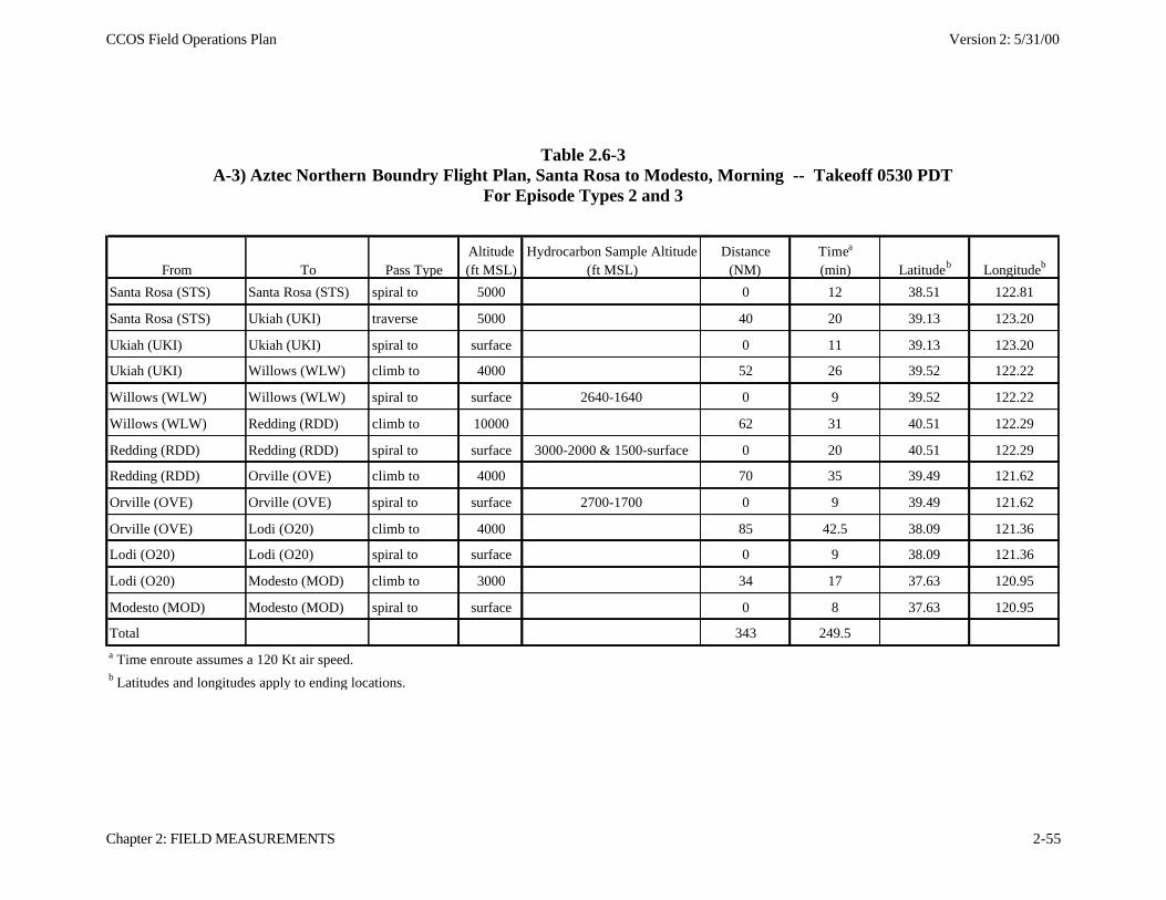
CCOS Field Operations Plan Version 2: 5/31/00
Chapter 2: FIELD MEASUREMENTS 2-55
Table 2.6-3A-3) Aztec Northern Boundry Flight Plan, Santa Rosa to Modesto, Morning -- Takeoff 0530 PDT
For Episode Types 2 and 3
From To Pass TypeAltitude (ft MSL)
Hydrocarbon Sample Altitude (ft MSL)
Distance (NM)
Timea
(min) Latitudeb Longitudeb
Santa Rosa (STS) Santa Rosa (STS) spiral to 5000 0 12 38.51 122.81
Santa Rosa (STS) Ukiah (UKI) traverse 5000 40 20 39.13 123.20
Ukiah (UKI) Ukiah (UKI) spiral to surface 0 11 39.13 123.20
Ukiah (UKI) Willows (WLW) climb to 4000 52 26 39.52 122.22
Willows (WLW) Willows (WLW) spiral to surface 2640-1640 0 9 39.52 122.22
Willows (WLW) Redding (RDD) climb to 10000 62 31 40.51 122.29
Redding (RDD) Redding (RDD) spiral to surface 3000-2000 & 1500-surface 0 20 40.51 122.29
Redding (RDD) Orville (OVE) climb to 4000 70 35 39.49 121.62
Orville (OVE) Orville (OVE) spiral to surface 2700-1700 0 9 39.49 121.62
Orville (OVE) Lodi (O20) climb to 4000 85 42.5 38.09 121.36
Lodi (O20) Lodi (O20) spiral to surface 0 9 38.09 121.36
Lodi (O20) Modesto (MOD) climb to 3000 34 17 37.63 120.95
Modesto (MOD) Modesto (MOD) spiral to surface 0 8 37.63 120.95
Total 343 249.5
a Time enroute assumes a 120 Kt air speed.b Latitudes and longitudes apply to ending locations.
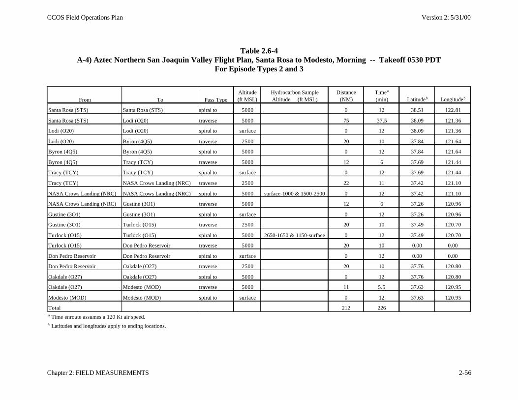
CCOS Field Operations Plan Version 2: 5/31/00
Chapter 2: FIELD MEASUREMENTS 2-56
Table 2.6-4A-4) Aztec Northern San Joaquin Valley Flight Plan, Santa Rosa to Modesto, Morning -- Takeoff 0530 PDT
For Episode Types 2 and 3
From To Pass TypeAltitude (ft MSL)
Hydrocarbon Sample Altitude (ft MSL)
Distance (NM)
Timea
(min) Latitudeb Longitudeb
Santa Rosa (STS) Santa Rosa (STS) spiral to 5000 0 12 38.51 122.81
Santa Rosa (STS) Lodi (O20) traverse 5000 75 37.5 38.09 121.36
Lodi (O20) Lodi (O20) spiral to surface 0 12 38.09 121.36
Lodi (O20) Byron (4Q5) traverse 2500 20 10 37.84 121.64
Byron (4Q5) Byron (4Q5) spiral to 5000 0 12 37.84 121.64
Byron (4Q5) Tracy (TCY) traverse 5000 12 6 37.69 121.44
Tracy (TCY) Tracy (TCY) spiral to surface 0 12 37.69 121.44
Tracy (TCY) NASA Crows Landing (NRC) traverse 2500 22 11 37.42 121.10
NASA Crows Landing (NRC) NASA Crows Landing (NRC) spiral to 5000 surface-1000 & 1500-2500 0 12 37.42 121.10
NASA Crows Landing (NRC) Gustine (3O1) traverse 5000 12 6 37.26 120.96
Gustine (3O1) Gustine (3O1) spiral to surface 0 12 37.26 120.96
Gustine (3O1) Turlock (O15) traverse 2500 20 10 37.49 120.70
Turlock (O15) Turlock (O15) spiral to 5000 2650-1650 & 1150-surface 0 12 37.49 120.70
Turlock (O15) Don Pedro Reservoir traverse 5000 20 10 0.00 0.00
Don Pedro Reservoir Don Pedro Reservoir spiral to surface 0 12 0.00 0.00
Don Pedro Reservoir Oakdale (O27) traverse 2500 20 10 37.76 120.80
Oakdale (O27) Oakdale (O27) spiral to 5000 0 12 37.76 120.80
Oakdale (O27) Modesto (MOD) traverse 5000 11 5.5 37.63 120.95
Modesto (MOD) Modesto (MOD) spiral to surface 0 12 37.63 120.95
Total 212 226a Time enroute assumes a 120 Kt air speed.b Latitudes and longitudes apply to ending locations.
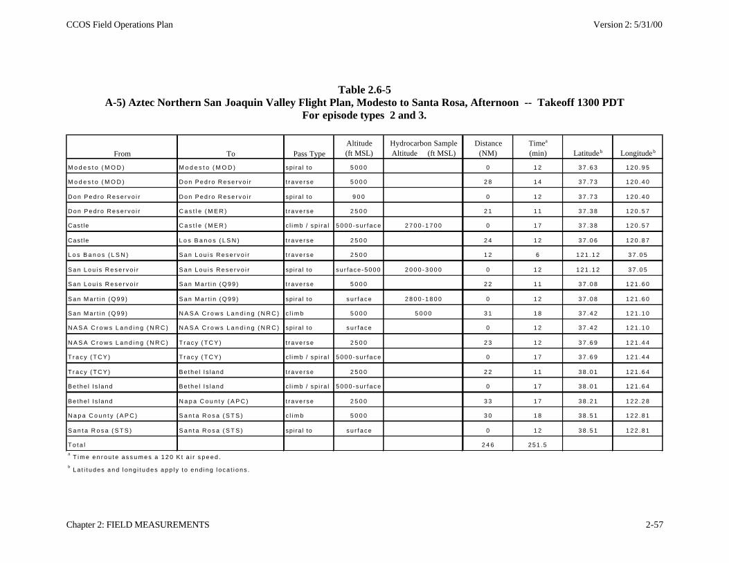
CCOS Field Operations Plan Version 2: 5/31/00
Chapter 2: FIELD MEASUREMENTS 2-57
Table 2.6-5A-5) Aztec Northern San Joaquin Valley Flight Plan, Modesto to Santa Rosa, Afternoon -- Takeoff 1300 PDT
For episode types 2 and 3.
From To Pass TypeAltitude (ft MSL)
Hydrocarbon Sample Altitude (ft MSL)
Distance (NM)
Timea
(min) Latitudeb Longitudeb
M o d e s t o ( M O D ) M o d e s t o ( M O D ) spi ra l to 5 0 0 0 0 1 2 3 7 . 6 3 1 2 0 . 9 5
M o d e s t o ( M O D ) D o n P e d r o R e s e r v o i r t r a v e r s e 5 0 0 0 2 8 1 4 3 7 . 7 3 1 2 0 . 4 0
D o n P e d r o R e s e r v o i r D o n P e d r o R e s e r v o i r sp i ra l to 9 0 0 0 1 2 3 7 . 7 3 1 2 0 . 4 0
D o n P e d r o R e s e r v o i r C a s t l e ( M E R ) t r a v e r s e 2 5 0 0 2 1 1 1 3 7 . 3 8 1 2 0 . 5 7
Cast le C a s t l e ( M E R ) c l imb / sp i ra l 5 0 0 0 - s u r f a c e 2 7 0 0 - 1 7 0 0 0 1 7 3 7 . 3 8 1 2 0 . 5 7
Cast le L o s B a n o s ( L S N ) t r a v e r s e 2 5 0 0 2 4 1 2 3 7 . 0 6 1 2 0 . 8 7
L o s B a n o s ( L S N ) S a n L o u i s R e s e r v o i r t r a v e r s e 2 5 0 0 1 2 6 1 2 1 . 1 2 3 7 . 0 5
S a n L o u i s R e s e r v o i r S a n L o u i s R e s e r v o i r sp i ra l to su r face -5000 2 0 0 0 - 3 0 0 0 0 1 2 1 2 1 . 1 2 3 7 . 0 5
S a n L o u i s R e s e r v o i r S a n M a r t i n ( Q 9 9 ) t r a v e r s e 5 0 0 0 2 2 1 1 3 7 . 0 8 1 2 1 . 6 0
S a n M a r t i n ( Q 9 9 ) S a n M a r t i n ( Q 9 9 ) spi ra l to s u r f a c e 2 8 0 0 - 1 8 0 0 0 1 2 3 7 . 0 8 1 2 1 . 6 0
S a n M a r t i n ( Q 9 9 ) N A S A C r o w s L a n d i n g ( N R C ) c l i m b 5 0 0 0 5 0 0 0 3 1 1 8 3 7 . 4 2 1 2 1 . 1 0
N A S A C r o w s L a n d i n g ( N R C ) N A S A C r o w s L a n d i n g ( N R C ) spi ra l to s u r f a c e 0 1 2 3 7 . 4 2 1 2 1 . 1 0
N A S A C r o w s L a n d i n g ( N R C ) T r a c y ( T C Y ) t r a v e r s e 2 5 0 0 2 3 1 2 3 7 . 6 9 1 2 1 . 4 4
T r a c y ( T C Y ) T r a c y ( T C Y ) c l imb / sp i ra l 5 0 0 0 - s u r f a c e 0 1 7 3 7 . 6 9 1 2 1 . 4 4
T r a c y ( T C Y ) Be the l I s l and t r a v e r s e 2 5 0 0 2 2 1 1 3 8 . 0 1 1 2 1 . 6 4
Be the l I s l and Be the l I s l and c l imb / sp i ra l 5 0 0 0 - s u r f a c e 0 1 7 3 8 . 0 1 1 2 1 . 6 4
Be the l I s l and N a p a C o u n t y ( A P C ) t r a v e r s e 2 5 0 0 3 3 1 7 3 8 . 2 1 1 2 2 . 2 8
N a p a C o u n t y ( A P C ) S a n t a R o s a ( S T S ) c l i m b 5 0 0 0 3 0 1 8 3 8 . 5 1 1 2 2 . 8 1
S a n t a R o s a ( S T S ) S a n t a R o s a ( S T S ) spi ra l to s u r f a c e 0 1 2 3 8 . 5 1 1 2 2 . 8 1
T o t a l 2 4 6 251 .5a T i m e e n r o u t e a s s u m e s a 1 2 0 K t a i r s p e e d .
b L a t i t u d e s a n d l o n g i t u d e s a p p l y t o e n d i n g l o c a t i o n s .
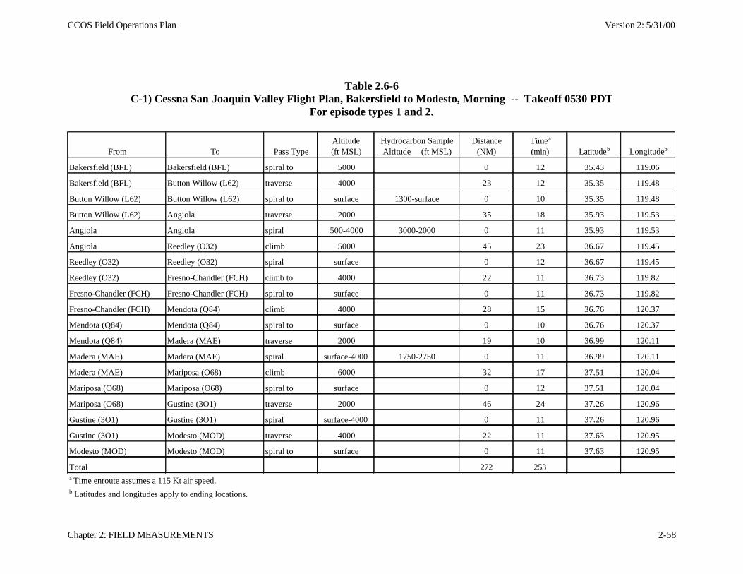
CCOS Field Operations Plan Version 2: 5/31/00
Chapter 2: FIELD MEASUREMENTS 2-58
Table 2.6-6C-1) Cessna San Joaquin Valley Flight Plan, Bakersfield to Modesto, Morning -- Takeoff 0530 PDT
For episode types 1 and 2.
From To Pass TypeAltitude (ft MSL)
Hydrocarbon Sample Altitude (ft MSL)
Distance (NM)
Timea
(min) Latitudeb Longitudeb
Bakersfield (BFL) Bakersfield (BFL) spiral to 5000 0 12 35.43 119.06
Bakersfield (BFL) Button Willow (L62) traverse 4000 23 12 35.35 119.48
Button Willow (L62) Button Willow (L62) spiral to surface 1300-surface 0 10 35.35 119.48
Button Willow (L62) Angiola traverse 2000 35 18 35.93 119.53
Angiola Angiola spiral 500-4000 3000-2000 0 11 35.93 119.53
Angiola Reedley (O32) climb 5000 45 23 36.67 119.45
Reedley (O32) Reedley (O32) spiral surface 0 12 36.67 119.45
Reedley (O32) Fresno-Chandler (FCH) climb to 4000 22 11 36.73 119.82
Fresno-Chandler (FCH) Fresno-Chandler (FCH) spiral to surface 0 11 36.73 119.82
Fresno-Chandler (FCH) Mendota (Q84) climb 4000 28 15 36.76 120.37
Mendota (Q84) Mendota (Q84) spiral to surface 0 10 36.76 120.37
Mendota (Q84) Madera (MAE) traverse 2000 19 10 36.99 120.11
Madera (MAE) Madera (MAE) spiral surface-4000 1750-2750 0 11 36.99 120.11
Madera (MAE) Mariposa (O68) climb 6000 32 17 37.51 120.04
Mariposa (O68) Mariposa (O68) spiral to surface 0 12 37.51 120.04
Mariposa (O68) Gustine (3O1) traverse 2000 46 24 37.26 120.96
Gustine (3O1) Gustine (3O1) spiral surface-4000 0 11 37.26 120.96
Gustine (3O1) Modesto (MOD) traverse 4000 22 11 37.63 120.95
Modesto (MOD) Modesto (MOD) spiral to surface 0 11 37.63 120.95
Total 272 253a Time enroute assumes a 115 Kt air speed.b Latitudes and longitudes apply to ending locations.
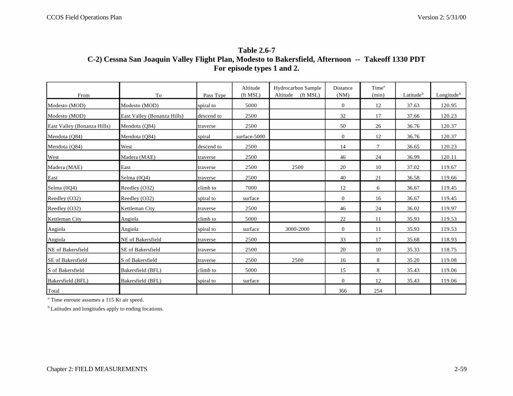
CCOS Field Operations Plan Version 2: 5/31/00
Chapter 2: FIELD MEASUREMENTS 2-59
Table 2.6-7C-2) Cessna San Joaquin Valley Flight Plan, Modesto to Bakersfield, Afternoon -- Takeoff 1330 PDT
For episode types 1 and 2.
From To Pass TypeAltitude (ft MSL)
Hydrocarbon Sample Altitude (ft MSL)
Distance (NM)
Timea
(min) Latitudeb Longitudeb
Modesto (MOD) Modesto (MOD) spiral to 5000 0 12 37.63 120.95
Modesto (MOD) East Valley (Bonanza Hills) descend to 2500 32 17 37.66 120.23
East Valley (Bonanza Hills) Mendota (Q84) traverse 2500 50 26 36.76 120.37
Mendota (Q84) Mendota (Q84) spiral surface-5000 0 12 36.76 120.37
Mendota (Q84) West descend to 2500 14 7 36.65 120.23
West Madera (MAE) traverse 2500 46 24 36.99 120.11
Madera (MAE) East traverse 2500 2500 20 10 37.02 119.67
East Selma (0Q4) traverse 2500 40 21 36.58 119.66
Selma (0Q4) Reedley (O32) climb to 7000 12 6 36.67 119.45
Reedley (O32) Reedley (O32) spiral to surface 0 16 36.67 119.45
Reedley (O32) Kettleman City traverse 2500 46 24 36.02 119.97
Kettleman City Angiola climb to 5000 22 11 35.93 119.53
Angiola Angiola spiral to surface 3000-2000 0 11 35.93 119.53
Angiola NE of Bakersfield traverse 2500 33 17 35.68 118.93
NE of Bakersfield SE of Bakersfield traverse 2500 20 10 35.33 118.75
SE of Bakersfield S of Bakersfield traverse 2500 2500 16 8 35.20 119.08
S of Bakersfield Bakersfield (BFL) climb to 5000 15 8 35.43 119.06
Bakersfield (BFL) Bakersfield (BFL) spiral to surface 0 12 35.43 119.06
Total 366 254a Time enroute assumes a 115 Kt air speed.b Latitudes and longitudes apply to ending locations.
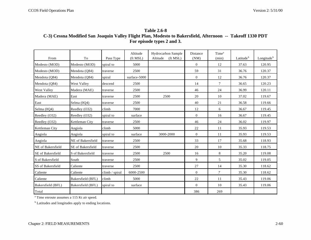
CCOS Field Operations Plan Version 2: 5/31/00
Chapter 2: FIELD MEASUREMENTS 2-60
Table 2.6-8C-3) Cessna Modified San Joaquin Valley Flight Plan, Modesto to Bakersfield, Afternoon -- Takeoff 1330 PDT
For episode types 2 and 3.
From To Pass TypeAltitude (ft MSL)
Hydrocarbon Sample Altitude (ft MSL)
Distance (NM)
Timea
(min) Latitudeb Longitudeb
Modesto (MOD) Modesto (MOD) spiral to 5000 0 12 37.63 120.95
Modesto (MOD) Mendota (Q84) traverse 2500 59 31 36.76 120.37
Mendota (Q84) Mendota (Q84) spiral surface-5000 0 12 36.76 120.37
Mendota (Q84) West Valley descend 2500 14 7 36.65 120.23
West Valley Madera (MAE) traverse 2500 46 24 36.99 120.11
Madera (MAE) East traverse 2500 2500 20 10 37.02 119.67
East Selma (0Q4) traverse 2500 40 21 36.58 119.66
Selma (0Q4) Reedley (O32) climb 7000 12 6 36.67 119.45
Reedley (O32) Reedley (O32) spiral to surface 0 16 36.67 119.45
Reedley (O32) Kettleman City traverse 2500 46 24 36.02 119.97
Kettleman City Angiola climb 5000 22 11 35.93 119.53
Angiola Angiola spiral to surface 3000-2000 0 11 35.93 119.53
Angiola NE of Bakersfield traverse 2500 33 17 35.68 118.93
NE of Bakersfield SE of Bakersfield traverse 2500 20 10 35.33 118.75
SE of Bakersfield S of Bakersfield traverse 2500 2500 16 8 35.20 119.08
S of Bakersfield South traverse 2500 9 5 35.02 119.05
SS of Bakersfield Caliente traverse 2500 27 14 35.30 118.62
Caliente Caliente climb / spiral 6000-2500 0 7 35.30 118.62
Caliente Bakersfield (BFL) climb 5000 22 11 35.43 119.06
Bakersfield (BFL) Bakersfield (BFL) spiral to surface 0 10 35.43 119.06
Total 386 269a Time enroute assumes a 115 Kt air speed.b Latitudes and longitudes apply to ending locations.
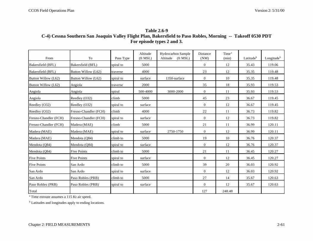
CCOS Field Operations Plan Version 2: 5/31/00
Chapter 2: FIELD MEASUREMENTS 2-61
Table 2.6-9C-4) Cessna Southern San Joaquin Valley Flight Plan, Bakersfield to Paso Robles, Morning -- Takeoff 0530 PDT
For episode types 2 and 3.
From To Pass TypeAltitude (ft MSL)
Hydrocarbon Sample Altitude (ft MSL)
Distance (NM)
Timea
(min) Latitudeb Longitudeb
Bakersfield (BFL) Bakersfield (BFL) spiral to 5000 0 12 35.43 119.06
Bakersfield (BFL) Button Willow (L62) traverse 4000 23 12 35.35 119.48
Button Willow (L62) Button Willow (L62) spiral to surface 1350-surface 0 10 35.35 119.48
Button Willow (L62) Angiola traverse 2000 35 18 35.93 119.53
Angiola Angiola spiral 500-4000 3000-2000 0 11 35.93 119.53
Angiola Reedley (O32) climb 5000 45 23 36.67 119.45
Reedley (O32) Reedley (O32) spiral to surface 0 12 36.67 119.45
Reedley (O32) Fresno-Chandler (FCH) climb 4000 22 11 36.73 119.82
Fresno-Chandler (FCH) Fresno-Chandler (FCH) spiral to surface 0 12 36.73 119.82
Fresno-Chandler (FCH) Madera (MAE) climb 5000 21 11 36.99 120.11
Madera (MAE) Madera (MAE) spiral to surface 2750-1750 0 12 36.99 120.11
Madera (MAE) Mendota (Q84) climb to 5000 19 10 36.76 120.37
Mendota (Q84) Mendota (Q84) spiral to surface 0 12 36.76 120.37
Mendota (Q84) Five Points climb to 5000 21 11 36.45 120.27
Five Points Five Points spiral to surface 0 12 36.45 120.27
Five Points San Ardo climb to 5000 39 20 36.03 120.92
San Ardo San Ardo spiral to surface 0 12 36.03 120.92
San Ardo Paso Robles (PRB) climb to 5000 27 14 35.67 120.63
Paso Robles (PRB) Paso Robles (PRB) spiral to surface 0 12 35.67 120.63
Total 127 248.48a Time enroute assumes a 115 Kt air speed.b Latitudes and longitudes apply to ending locations.
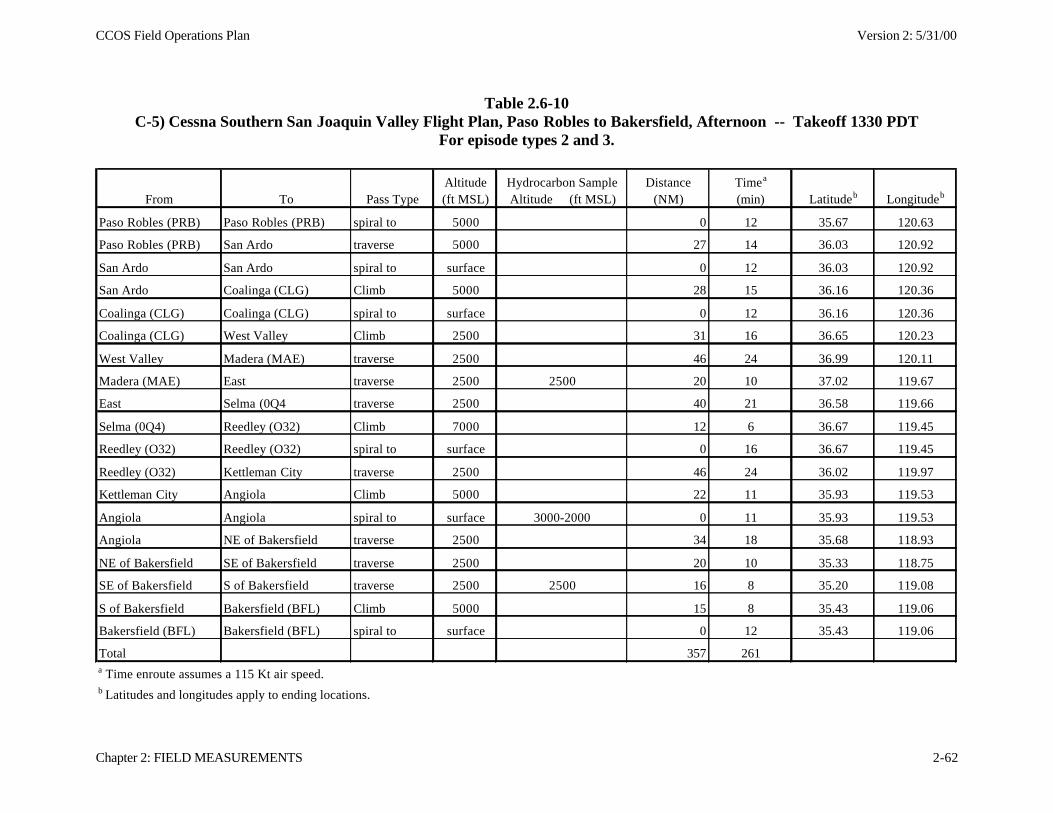
CCOS Field Operations Plan Version 2: 5/31/00
Chapter 2: FIELD MEASUREMENTS 2-62
Table 2.6-10C-5) Cessna Southern San Joaquin Valley Flight Plan, Paso Robles to Bakersfield, Afternoon -- Takeoff 1330 PDT
For episode types 2 and 3.
From To Pass TypeAltitude (ft MSL)
Hydrocarbon Sample Altitude (ft MSL)
Distance (NM)
Timea
(min) Latitudeb Longitudeb
Paso Robles (PRB) Paso Robles (PRB) spiral to 5000 0 12 35.67 120.63
Paso Robles (PRB) San Ardo traverse 5000 27 14 36.03 120.92
San Ardo San Ardo spiral to surface 0 12 36.03 120.92
San Ardo Coalinga (CLG) Climb 5000 28 15 36.16 120.36
Coalinga (CLG) Coalinga (CLG) spiral to surface 0 12 36.16 120.36
Coalinga (CLG) West Valley Climb 2500 31 16 36.65 120.23
West Valley Madera (MAE) traverse 2500 46 24 36.99 120.11
Madera (MAE) East traverse 2500 2500 20 10 37.02 119.67
East Selma (0Q4 traverse 2500 40 21 36.58 119.66
Selma (0Q4) Reedley (O32) Climb 7000 12 6 36.67 119.45
Reedley (O32) Reedley (O32) spiral to surface 0 16 36.67 119.45
Reedley (O32) Kettleman City traverse 2500 46 24 36.02 119.97
Kettleman City Angiola Climb 5000 22 11 35.93 119.53
Angiola Angiola spiral to surface 3000-2000 0 11 35.93 119.53
Angiola NE of Bakersfield traverse 2500 34 18 35.68 118.93
NE of Bakersfield SE of Bakersfield traverse 2500 20 10 35.33 118.75
SE of Bakersfield S of Bakersfield traverse 2500 2500 16 8 35.20 119.08
S of Bakersfield Bakersfield (BFL) Climb 5000 15 8 35.43 119.06
Bakersfield (BFL) Bakersfield (BFL) spiral to surface 0 12 35.43 119.06
Total 357 261a Time enroute assumes a 115 Kt air speed.b Latitudes and longitudes apply to ending locations.
CCOS Field Operations Plan Version 2: 5/31/00
Chapter 2: FIELD MEASUREMENTS 2-63
2.6.5 Pacific Northwest National Laboratory Gulfstream 159 (G-1)
Aircraft: Twin engine turboprop
Measurements: Position (Trimble GSP/Loran C); temperature (Rosemount), pressure(Rosemount), wind (differential pressure gust probe and GPS), humidity (General Eastern chilledmirror; AIR Lyman-α), SO2 (TEI 43S), O3 (TEI 49-100), CO (TEI 48), particle size spectrum(PMS FSSP & PCASP-100X), particle concentration (TSI 3010), particle optical properties (TSI3563 nephelometer, Radiance PSAP), PAN/NO2 (ANL), formaldehyde (BNL), up/down totalUV (Eppley TUV), HC canisters (ANL)
Note: ARB has agreed to provide a TEI 42S NO/NOy instrument for use during CCOS butdelivery date has not been confirmed.
Hours Budgeted: ~60 hours including ferry time.
Base Airport: Fresno Air Terminal
Area of Coverage: South-central San Joaquin Valley, mainly Fresno area. West of San Franciscoover the Pacific Ocean to sample western in-flow boundary conditions.
Operational Constraints: Because the G-1 is considered a "heavy" aircraft, low altitudeoperations are governed by the provisions of the PNNL Flight Operations Manual (MA-530) anda waiver by the FAA of regulation 91.119(c). The waiver and our low-level operations manualwill be submitted for the purview of the Oakland Flight Standards District Office. Permissionswill be requested from the applicable agencies for low level flight for periods of 10-12 minutesdown to 300 ft AGL over water within the boundaries of the offshore marine sanctuaries and forperiods of less than 5 minutes down to 500 ft AGL over inland wildlife sanctuaries along theflight paths described below.
Quality Assurance Audits: Coordinate with ARB quality assurance section for audit on 7/6/00 inFresno.
Data Comparison: The far higher sampling speed of the G-1 makes in-flight comparisons withother CCOS aircraft ineffective use of flight time. Ground audits by ARB of G-1 instrumentswill be needed to establish data comparability. When practical, the G-1 will fly by the Angiolatower and radar wind profilers.
Flight Plans: There are two sets of basic flight plans for the G-1 in CCOS: 1) Fresno and centralSan Joaquin Valley and 2) Western In-Flow Boundary. Within each there are separate morningand afternoon flight patterns. Timing of the morning and afternoon flights has to take intoaccount the length of the duty day for the pilots (<12 hours) as well as the scientific objectivesfor each flight. Even with activation of our FAA Low-Level Waiver, operations below 1000 ftAGL over populated areas can only be done over an airport. Portions of the ferry flights betweenPasco, WA and Fresno, CA, may be useful for sampling within the Central Valley; flight planswill be arranged at a later date.
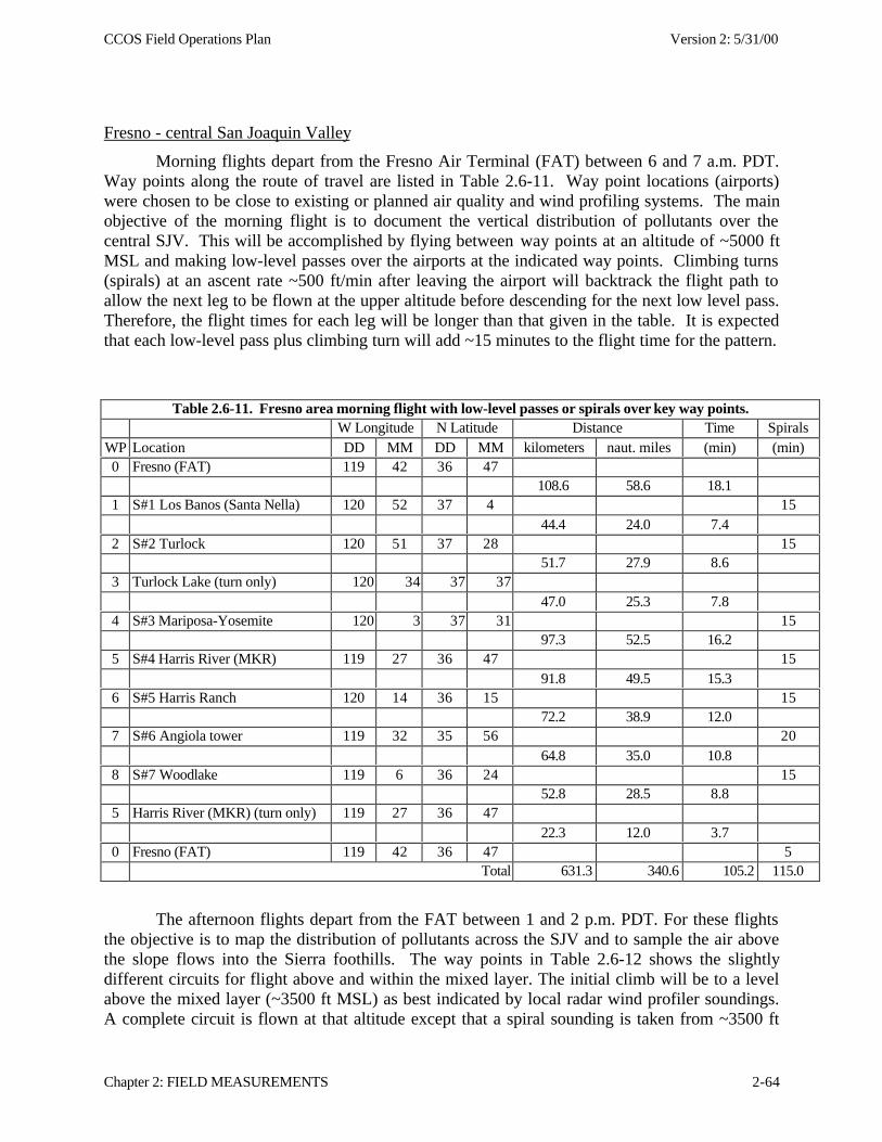
CCOS Field Operations Plan Version 2: 5/31/00
Chapter 2: FIELD MEASUREMENTS 2-64
Fresno - central San Joaquin Valley
Morning flights depart from the Fresno Air Terminal (FAT) between 6 and 7 a.m. PDT.Way points along the route of travel are listed in Table 2.6-11. Way point locations (airports)were chosen to be close to existing or planned air quality and wind profiling systems. The mainobjective of the morning flight is to document the vertical distribution of pollutants over thecentral SJV. This will be accomplished by flying between way points at an altitude of ~5000 ftMSL and making low-level passes over the airports at the indicated way points. Climbing turns(spirals) at an ascent rate ~500 ft/min after leaving the airport will backtrack the flight path toallow the next leg to be flown at the upper altitude before descending for the next low level pass.Therefore, the flight times for each leg will be longer than that given in the table. It is expectedthat each low-level pass plus climbing turn will add ~15 minutes to the flight time for the pattern.
Table 2.6-11. Fresno area morning flight with low-level passes or spirals over key way points.W Longitude N Latitude Distance Time Spirals
WP Location DD MM DD MM kilometers naut. miles (min) (min)0 Fresno (FAT) 119 42 36 47
108.6 58.6 18.11 S#1 Los Banos (Santa Nella) 120 52 37 4 15
44.4 24.0 7.42 S#2 Turlock 120 51 37 28 15
51.7 27.9 8.63 Turlock Lake (turn only) 120 34 37 37
47.0 25.3 7.84 S#3 Mariposa-Yosemite 120 3 37 31 15
97.3 52.5 16.25 S#4 Harris River (MKR) 119 27 36 47 15
91.8 49.5 15.36 S#5 Harris Ranch 120 14 36 15 15
72.2 38.9 12.07 S#6 Angiola tower 119 32 35 56 20
64.8 35.0 10.88 S#7 Woodlake 119 6 36 24 15
52.8 28.5 8.85 Harris River (MKR) (turn only) 119 27 36 47
22.3 12.0 3.70 Fresno (FAT) 119 42 36 47 5
Total 631.3 340.6 105.2 115.0
The afternoon flights depart from the FAT between 1 and 2 p.m. PDT. For these flightsthe objective is to map the distribution of pollutants across the SJV and to sample the air abovethe slope flows into the Sierra foothills. The way points in Table 2.6-12 shows the slightlydifferent circuits for flight above and within the mixed layer. The initial climb will be to a levelabove the mixed layer (~3500 ft MSL) as best indicated by local radar wind profiler soundings.A complete circuit is flown at that altitude except that a spiral sounding is taken from ~3500 ft
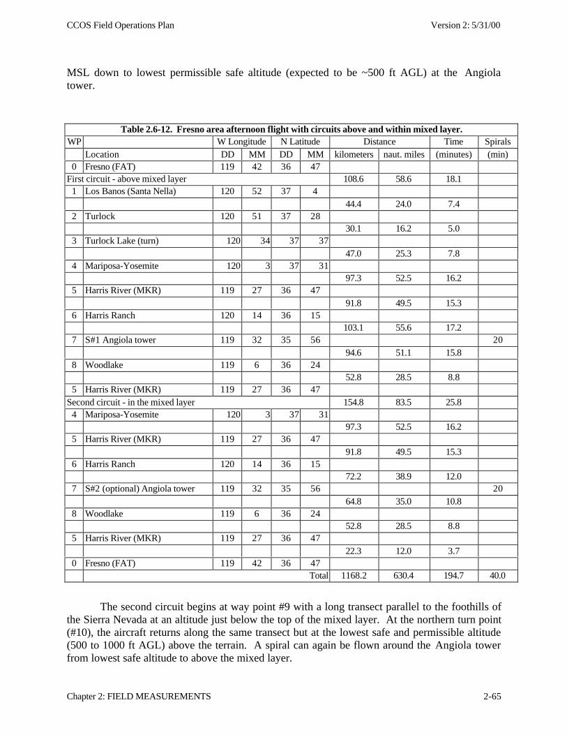
CCOS Field Operations Plan Version 2: 5/31/00
Chapter 2: FIELD MEASUREMENTS 2-65
MSL down to lowest permissible safe altitude (expected to be ~500 ft AGL) at the Angiolatower.
Table 2.6-12. Fresno area afternoon flight with circuits above and within mixed layer.WP W Longitude N Latitude Distance Time Spirals
Location DD MM DD MM kilometers naut. miles (minutes) (min)0 Fresno (FAT) 119 42 36 47
First circuit - above mixed layer 108.6 58.6 18.11 Los Banos (Santa Nella) 120 52 37 4
44.4 24.0 7.42 Turlock 120 51 37 28
30.1 16.2 5.03 Turlock Lake (turn) 120 34 37 37
47.0 25.3 7.84 Mariposa-Yosemite 120 3 37 31
97.3 52.5 16.25 Harris River (MKR) 119 27 36 47
91.8 49.5 15.36 Harris Ranch 120 14 36 15
103.1 55.6 17.27 S#1 Angiola tower 119 32 35 56 20
94.6 51.1 15.88 Woodlake 119 6 36 24
52.8 28.5 8.85 Harris River (MKR) 119 27 36 47
Second circuit - in the mixed layer 154.8 83.5 25.84 Mariposa-Yosemite 120 3 37 31
97.3 52.5 16.25 Harris River (MKR) 119 27 36 47
91.8 49.5 15.36 Harris Ranch 120 14 36 15
72.2 38.9 12.07 S#2 (optional) Angiola tower 119 32 35 56 20
64.8 35.0 10.88 Woodlake 119 6 36 24
52.8 28.5 8.85 Harris River (MKR) 119 27 36 47
22.3 12.0 3.70 Fresno (FAT) 119 42 36 47
Total 1168.2 630.4 194.7 40.0
The second circuit begins at way point #9 with a long transect parallel to the foothills ofthe Sierra Nevada at an altitude just below the top of the mixed layer. At the northern turn point(#10), the aircraft returns along the same transect but at the lowest safe and permissible altitude(500 to 1000 ft AGL) above the terrain. A spiral can again be flown around the Angiola towerfrom lowest safe altitude to above the mixed layer.
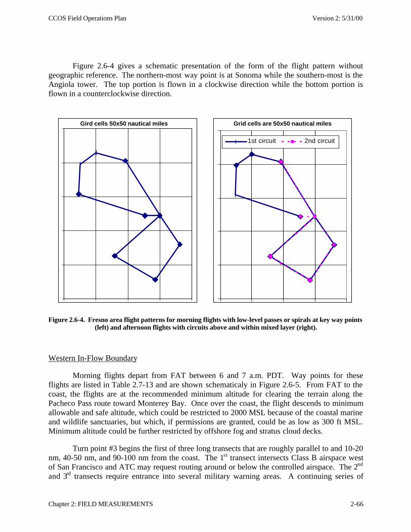
CCOS Field Operations Plan Version 2: 5/31/00
Chapter 2: FIELD MEASUREMENTS 2-66
Figure 2.6-4 gives a schematic presentation of the form of the flight pattern withoutgeographic reference. The northern-most way point is at Sonoma while the southern-most is theAngiola tower. The top portion is flown in a clockwise direction while the bottom portion isflown in a counterclockwise direction.
Figure 2.6-4. Fresno area flight patterns for morning flights with low-level passes or spirals at key way points(left) and afternoon flights with circuits above and within mixed layer (right).
Western In-Flow Boundary
Morning flights depart from FAT between 6 and 7 a.m. PDT. Way points for theseflights are listed in Table 2.7-13 and are shown schematicaly in Figure 2.6-5. From FAT to thecoast, the flights are at the recommended minimum altitude for clearing the terrain along thePacheco Pass route toward Monterey Bay. Once over the coast, the flight descends to minimumallowable and safe altitude, which could be restricted to 2000 MSL because of the coastal marineand wildlife sanctuaries, but which, if permissions are granted, could be as low as 300 ft MSL.Minimum altitude could be further restricted by offshore fog and stratus cloud decks.
Turn point #3 begins the first of three long transects that are roughly parallel to and 10-20nm, 40-50 nm, and 90-100 nm from the coast. The 1st transect intersects Class B airspace westof San Francisco and ATC may request routing around or below the controlled airspace. The 2nd
and 3rd transects require entrance into several military warning areas. A continuing series of
Grid cells are 50x50 nautical miles
1st circuit 2nd circuit
Gird cells 50x50 nautical miles
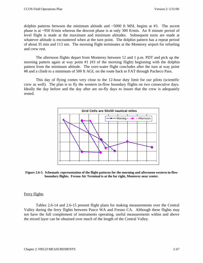
CCOS Field Operations Plan Version 2: 5/31/00
Chapter 2: FIELD MEASUREMENTS 2-67
dolphin patterns between the minimum altitude and ~5000 ft MSL begins at #3. The ascentphase is at ~950 ft/min whereas the descent phase is at only 300 ft/min. An 8 minute period oflevel flight is made at the maximum and minimum altitudes. Subsequent turns are made atwhatever altitude is encountered when at the turn point. The dolphin pattern has a repeat periodof about 35 min and 113 nm. The morning flight terminates at the Monterey airport for refuelingand crew rest.
The afternoon flights depart from Monterey between 12 and 1 p.m. PDT and pick up themorning pattern again at way point #1 (#3 of the morning flight) beginning with the dolphinpattern from the minimum altitude. The over-water flight concludes after the turn at way point#8 and a climb to a minimum of 500 ft AGL on the route back to FAT through Pacheco Pass.
This day of flying comes very close to the 12-hour duty limit for our pilots (scientificcrew as well). The plan is to fly the western in-flow boundary flights on two consecutive days.Ideally the day before and the day after are no-fly days to insure that the crew is adequatelyrested.
Figure 2.6-5. Schematic representation of the flight patterns for the morning and afternoon western in-flowboundary flights. Fresno Air Terminal is at the far right, Monterey near center.
Ferry flights
Tables 2.6-14 and 2.6-15 present flight plans for making measurements over the CentralValley during the ferry flights between Pasco WA and Fresno CA. Although these flights maynot have the full complement of instruments operating, useful measurements within and abovethe mixed layer can be obtained over much of the length of the Central Valley.
Grid Cells are 50x50 nautical miles
Morning Afternoon
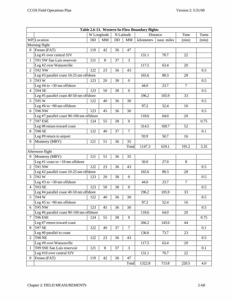
CCOS Field Operations Plan Version 2: 5/31/00
Chapter 2: FIELD MEASUREMENTS 2-68
Table 2.6-13. Western In-Flow Boundary flightsW Longitude N Latitude Distance Time Turns
WP Location DD MM DD MM kilometers naut. miles (min) (min)Morning flight
0 Fresno (FAT) 119 42 36 47Leg #1 over central SJV 131.1 70.7 22
1 T#1 SW San Luis reservoir 121 8 37 3Leg #2 over Watsonville 117.5 63.4 20
2 T#2 NW 122 23 36 43 0.5Leg #3 parallel coast 10-25 nm offshore 165.6 89.3 28
3 T#3 W 123 20 38 0 0.5Leg #4 to ~30 nm offshore 44.0 23.7 7
4 T#4 SE 123 50 38 0 0.5Leg #5 parallel coast 40-50 nm offshore 196.2 105.9 33
5 T#5 W 122 40 36 30 0.5Leg #6 to ~90 nm offshore 97.2 52.4 16
6 T#6 NW 123 45 36 30 0.5Leg #7 parallel coast 90-100 nm offshore 118.6 64.0 20
7 T#7 ESE 124 55 38 0 0.75Leg #8 return toward coast 314.5 169.7 52
8 T#8 SE 122 40 37 7 0.1Leg #9 return to airport 93.9 50.7 16
9 Monterey (MRY) 121 51 36 35Total 1147.3 619.1 191.2 3.35
Afternoon flight9 Monterey (MRY) 121 51 36 35
Leg #1 coast to ~18 nm offshore 50.0 27.0 82 T#1 NW 122 23 36 43 0.5
Leg #2 parallel coast 10-25 nm offshore 165.6 89.3 283 T#2 W 123 20 38 0 0.5
Leg #3 to ~30 nm offshore 44.0 23.7 74 T#3 SE 123 50 38 0 0.5
Leg #4 parallel coast 40-50 nm offshore 196.2 105.9 335 T#4 W 122 40 36 30 0.5
Leg #5 to ~90 nm offshore 97.2 52.4 166 T#5 NW 123 45 36 30 0.5
Leg #6 parallel coast 90-100 nm offshore 118.6 64.0 207 T#6 ESE 124 55 38 0 0.75
Leg #7 return toward coast 266.2 143.6 448 T#7 SE 122 40 37 7 0.1
Leg #8 parallel to coast 136.6 73.7 232 T#8 NE 122 23 36 43 0.5
Leg #9 over Watsonville 117.5 63.4 201 T#9 SSE San Luis reservoir 121 8 37 3 0.1
Leg #10 over central SJV 131.1 70.7 220 Fresno (FAT) 119 42 36 47
Total 1322.8 713.8 220.5 4.0
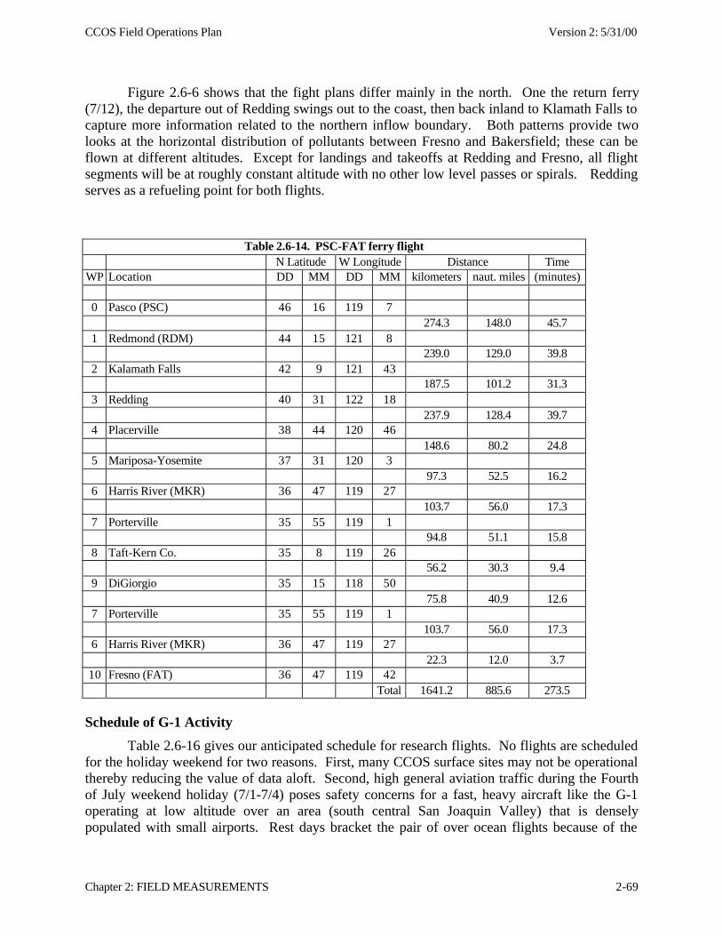
CCOS Field Operations Plan Version 2: 5/31/00
Chapter 2: FIELD MEASUREMENTS 2-69
Figure 2.6-6 shows that the fight plans differ mainly in the north. One the return ferry(7/12), the departure out of Redding swings out to the coast, then back inland to Klamath Falls tocapture more information related to the northern inflow boundary. Both patterns provide twolooks at the horizontal distribution of pollutants between Fresno and Bakersfield; these can beflown at different altitudes. Except for landings and takeoffs at Redding and Fresno, all flightsegments will be at roughly constant altitude with no other low level passes or spirals. Reddingserves as a refueling point for both flights.
Table 2.6-14. PSC-FAT ferry flightN Latitude W Longitude Distance Time
WP Location DD MM DD MM kilometers naut. miles (minutes)
0 Pasco (PSC) 46 16 119 7274.3 148.0 45.7
1 Redmond (RDM) 44 15 121 8239.0 129.0 39.8
2 Kalamath Falls 42 9 121 43187.5 101.2 31.3
3 Redding 40 31 122 18237.9 128.4 39.7
4 Placerville 38 44 120 46148.6 80.2 24.8
5 Mariposa-Yosemite 37 31 120 397.3 52.5 16.2
6 Harris River (MKR) 36 47 119 27103.7 56.0 17.3
7 Porterville 35 55 119 194.8 51.1 15.8
8 Taft-Kern Co. 35 8 119 2656.2 30.3 9.4
9 DiGiorgio 35 15 118 5075.8 40.9 12.6
7 Porterville 35 55 119 1103.7 56.0 17.3
6 Harris River (MKR) 36 47 119 2722.3 12.0 3.7
10 Fresno (FAT) 36 47 119 42Total 1641.2 885.6 273.5
Schedule of G-1 Activity
Table 2.6-16 gives our anticipated schedule for research flights. No flights are scheduledfor the holiday weekend for two reasons. First, many CCOS surface sites may not be operationalthereby reducing the value of data aloft. Second, high general aviation traffic during the Fourthof July weekend holiday (7/1-7/4) poses safety concerns for a fast, heavy aircraft like the G-1operating at low altitude over an area (south central San Joaquin Valley) that is denselypopulated with small airports. Rest days bracket the pair of over ocean flights because of the
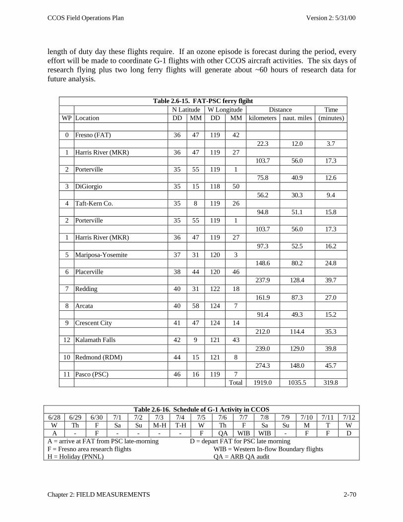
CCOS Field Operations Plan Version 2: 5/31/00
Chapter 2: FIELD MEASUREMENTS 2-70
length of duty day these flights require. If an ozone episode is forecast during the period, everyeffort will be made to coordinate G-1 flights with other CCOS aircraft activities. The six days ofresearch flying plus two long ferry flights will generate about ~60 hours of research data forfuture analysis.
Table 2.6-15. FAT-PSC ferry flgihtN Latitude W Longitude Distance Time
WP Location DD MM DD MM kilometers naut. miles (minutes)
0 Fresno (FAT) 36 47 119 4222.3 12.0 3.7
1 Harris River (MKR) 36 47 119 27103.7 56.0 17.3
2 Porterville 35 55 119 175.8 40.9 12.6
3 DiGiorgio 35 15 118 5056.2 30.3 9.4
4 Taft-Kern Co. 35 8 119 2694.8 51.1 15.8
2 Porterville 35 55 119 1103.7 56.0 17.3
1 Harris River (MKR) 36 47 119 2797.3 52.5 16.2
5 Mariposa-Yosemite 37 31 120 3148.6 80.2 24.8
6 Placerville 38 44 120 46237.9 128.4 39.7
7 Redding 40 31 122 18161.9 87.3 27.0
8 Arcata 40 58 124 791.4 49.3 15.2
9 Crescent City 41 47 124 14212.0 114.4 35.3
12 Kalamath Falls 42 9 121 43239.0 129.0 39.8
10 Redmond (RDM) 44 15 121 8274.3 148.0 45.7
11 Pasco (PSC) 46 16 119 7Total 1919.0 1035.5 319.8
Table 2.6-16. Schedule of G-1 Activity in CCOS6/28 6/29 6/30 7/1 7/2 7/3 7/4 7/5 7/6 7/7 7/8 7/9 7/10 7/11 7/12W Th F Sa Su M-H T-H W Th F Sa Su M T WA - F - - - - F QA WIB WIB - F F D
A = arrive at FAT from PSC late-morning D = depart FAT for PSC late morningF = Fresno area research flights WIB = Western In-flow Boundary flightsH = Holiday (PNNL) QA = ARB QA audit
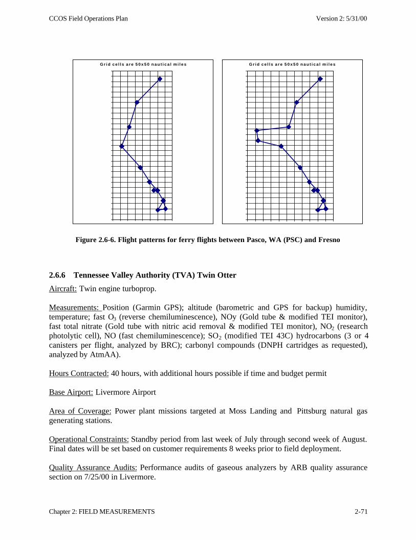
CCOS Field Operations Plan Version 2: 5/31/00
Chapter 2: FIELD MEASUREMENTS 2-71
Figure 2.6-6. Flight patterns for ferry flights between Pasco, WA (PSC) and Fresno
2.6.6 Tennessee Valley Authority (TVA) Twin Otter
Aircraft: Twin engine turboprop.
Measurements: Position (Garmin GPS); altitude (barometric and GPS for backup) humidity,temperature; fast O3 (reverse chemiluminescence), NOy (Gold tube & modified TEI monitor),fast total nitrate (Gold tube with nitric acid removal & modified TEI monitor), NO2 (researchphotolytic cell), NO (fast chemiluminescence); SO2 (modified TEI 43C) hydrocarbons (3 or 4canisters per flight, analyzed by BRC); carbonyl compounds (DNPH cartridges as requested),analyzed by AtmAA).
Hours Contracted: 40 hours, with additional hours possible if time and budget permit
Base Airport: Livermore Airport
Area of Coverage: Power plant missions targeted at Moss Landing and Pittsburg natural gasgenerating stations.
Operational Constraints: Standby period from last week of July through second week of August.Final dates will be set based on customer requirements 8 weeks prior to field deployment.
Quality Assurance Audits: Performance audits of gaseous analyzers by ARB quality assurancesection on 7/25/00 in Livermore.
G r i d c e l l s a r e 5 0 x 5 0 n a u t i c a l m i l e s G r i d c e l l s a r e 5 0 x 5 0 n a u t i c a l m i l e s
CCOS Field Operations Plan Version 2: 5/31/00
Chapter 2: FIELD MEASUREMENTS 2-72
Data Comparisons: Coordinate parallel flight with other aircraft as desired. TVA onboardcalibrator can be used to intercompare with other aircraft when at the same airport.
Flight Plans:Flight air speed will be near 125 kts for ferries and near 95 kts for plume traversing. Ferries willalso provide detailed gaseous speciation. Start time may be adjusted depending on expectedplume transport speed.
(1) Power Plant Mission: At 1100 PDT ferry from Livermore to target plant (Pittsburg orMoss Landing) at mid boundary layer. Spiral from minimum safe altitude to 5000’ 5 kmupwind of plant for upwind vertical profile. Circle plant at 5 km to establish actual plumecenterline direction and for first traverse. Continue a series of plume traverses at midboundary level at 5 km spacing out to distance where ozone chemistry has finished orplume is indistinguishable from background. Spacing of lagrangian plume traverses willbe fixed for a given flight and set based on profiler mid boundary layer wind at flighttime. Length of traverses will be adjusted in flight depending on horizontal mixingobserved in real time. Downwind spiral to 5000’ will be performed when last traversecompleted. Ferry back to Livermore airport at completion.
(2) Supplemental Mission: As time and existing budget permits TVA Twin Otter may addregional survey legs to power plant missions to enhance data in the Livermore Valley,Sacramento Valley or SJV as desired for clusters 1, 2, or 3 to increase detail andparameters measured by collaborating aircraft. Basing at Livermore should permitefficient add-ons. Detailed NOy speciation can greatly improve knowledge of chemicalage and processing of ozone rich airmasses. Supplemental missions will be coordinated atdaily planning sessions.
Objectives and Rationale: Map detailed ozone, precursor, and products in power plant plumesand in regional airmasses during ferries and supplemental add-ons.
2.6.7 VOC Sample Collection Methods and Protocols
Hydrocarbon samples are collected in stainless steel canisters and will be analyzed for C1
to C11 hydrocarbons, CO and CO2 at Biospheric Research Corporation (Beaverton, OR) by gaschromatography with flame ionization detection. The aircraft samplers will be supplied by BRC.They will operate manually off 24-48 volts and be configured to collect 3.2 liters canisters overaveraging times of several minutes to near instantaneous.
Carbonyl samples are collected in Tedlar bags and transferred to dinitrophenyl hydrazineimpregnated cartridges on the ground at the conclusion of the flight. Samples will be collectedby ramming air through a Telfon inlet tube into pre-cleaned 40-liter Tedlar bags that had beendoped with excess NO to react with any O3 in the air sample. Sampling times are approximately2-5 minutes. The stainless steel valves attached to the Teflon bags are specially modified topermit rapid filling and all rubber seals have been replaced with inert Viton parts. Because thesample sizes for the aloft carbonyl samples (nominally 30 liters) are substantially less than for atypical surface sample, additional efforts are necessary to reduce blank variability in order to
CCOS Field Operations Plan Version 2: 5/31/00
Chapter 2: FIELD MEASUREMENTS 2-73
achieve the required detection level. The samples will be analyzed for C1-C7 carbonylcompounds by HPLC with UV detection at AtmAA (Calabasas, CA).
The budget allows for collection and analysis of three or four sets of hydrocarbon andcarbonyl samples per flight.
2.6.8 Intercomparison Flights
Intercomparison flights will be performed between (1) the STI Aztec and STI Cessna182, (2) the two UCD Cessnas, (3) the STI 182 and one UCD Cessna, (4) the STI Aztec and theDOE G-1, and (5) one UCD Cessna and the TVA Twin Otter. The first three comparisons willbe made near Sacramento, the fourth near Fresno, and the fifth near Livermore. Each aircraft willcollect hydrocarbon and carbonyl samples in a clean location so that investigators can ensure thattheir sampling systems do not contaminate the samples. This can be done as part of theintercomparison flights or during initial test flights.
The intercomparison flights will compare measurements of ozone, NO, NOy, CO (whenavailable) temperature, relative humidity or dew point, and winds (when available). The aircraftwill compare clocks and GPS position systems on the ground prior to flight in order to facilitatesubsequent data processing and analysis. Flights will include spirals up and down to documenthysteresis and altitude effects, and will include traverses in the mixed layer and above the mixedlayer to compare measured concentrations at varying concentration levels. The flights will bemade downwind of urban areas in the mid-afternoon to increase the probability of encounteringelevated ozone and NOy concentrations.
The first four comparisons listed above will include comparisons of wind measurements.These flights will involve a dog-leg pattern at at least one of the traverse altitudes in order to testwhether the aircraft indicate the same winds using the orthogonal components of their windmeasuring devices.
Comparison 1 will start from STI’s base at Santa Rosa Airport (STS). Comparisons 2and 3 will start from the UCD’s base at University Airport (0O5) at Davis. Comparison 4 willstart at the DOE base at Fresno Yosemite International Airport (FAT). Comparison 5 will startat the TVA base at Livermore (LVK). Before each flight the aircraft will meet at the startingairports to synchronize data system clocks, compare GPS position readings, and to coordinateflight plans among the pilots. The flights will include a spiral up from an airport to 5000 ft mslor more with one following the other about 500 ft apart and a similar spiral back down to about2000 ft msl or less. The flights will also include a traverse at 2000-3000 ft msl along a path tointersect the local urban plume and a similar traverse at about 5000 ft msl or more. The aircraftwill fly the traverses side by side for at least 20 NM.
For comparisons 1 through 3, the aircraft will climb from their starting airports to 5500 ftover University Airport. From there they will traverse side-by-side at 5500 ft msl to SunsetSkyranch (Q40, 23 NM) and then to Auburn Airport (AUN, 35 NM). Over Auburn, they willdescend to 3000 ft msl, then traverse together at 3000 ft to Sunset Skyranch and then toSacramento Executive (SAC, 10 NM). Over Sacramento, they will descend and do a low pass
CCOS Field Operations Plan Version 2: 5/31/00
Chapter 2: FIELD MEASUREMENTS 2-74
over the airport, then spiral up to 5000 ft msl and spiral down to 2000 ft msl or below, beforereturning to their base airports.
For comparison 4 the aircraft will start at Fresno Yosemite Airport (FAT). The aircraftwill climb to 5000 ft msl over either Harris River (13 NM) or Reedley (O32, 15 NM), then spiraldown to the surface and back up to 6500 ft msl. The choice between Harris River and Reedleywill depend on whether permission can be obtained to do a low pass at Harris River which isprivate. They will then traverse to Mariposa-Yosemite Airport (O68, 54 NM) at 6500 ft msl,descend to 3000 ft msl at a point about 10 NM SW of Mariposa, traverse back to Harris River(54 NM) (or Reedley) and then to Harris Ranch (3O8, 49 NM) at 3000 ft MSL. From HarrisRanch, the DOE G-1 will continue on its afternoon flight plan, and the STI Aztec will return toSanta Rosa.
Comparisons 1 through 3 will take place the week of June 26th. Comparison 4 isscheduled for July 5. Comparison 5 will take place soon after TVA’s QA audit on July 25. Theflight plan details for comparison 5 will be worked out between UCD and TVA after the earliercomparison flights are evaluated, in case changes in approach are needed.
Data from the comparison flights should be processed, discussed between theinvestigators, and sent to DRI and ARB for review within one week after the flights.
CCOS Field Operations Plan Version 2: 5/31/00
Chapter 3: FORECAST PROTOCOL 3-1
3.0 FORECAST AND IOP DECISION PROTOCOL
The decision to declare an IOP will be based on daily meteorological and air qualityforecasts, and other information on current conditions and operational status. IntensiveOperational Periods (IOP) will be forecasted during periods that correspond to categories ofmeteorological conditions called scenarios, which are associated with ozone episodes and ozonetransport in northern and central California. This section describes the meteorological scenariosof interest in CCOS and the protocols for forecasting and decision-making.
3.1 Ozone Episode and Transport Scenarios of Interest
The classifications of ozone episodes in central and northern California are based uponidentification of meteorological scenarios that foster the formation, accumulation and transportof ozone within the CCOS area. The goals of the CCOS Meteorological Working Group(MetWG) are to identify and characterize these meteorological scenarios, and to develop andevaluate suitable forecasting tools and protocol. Toward this end, the MetWG examined ozoneepisodes for three ozone seasons, May-October, 1996-1998. Subjective classification byinspection of Daily Weather Maps was compared to the objective classification technique ofcluster analysis.
Previous investigators have used classification techniques varying from subjectiveinspection of weather charts (ETL 1994) and streamline plots (Hayes et al. 1984; Stoeckenius etal. 1994), to objective classification methods like linear regression (Roberts 1992), multivariateregression (Stoeckenius 1998), cluster analysis (Roberts et al. 1994; Smith 1994; Stoeckenius1994; Fairley and De Mandel 1996), empirical orthogonal functions (Ludwig et al. 1995) andneural networks (Stoeckenius, 1998). A more detailed discussion is provided by Fujita et al.(1999). In each of the cited cluster analyses, the number and nature of the clusters has varied.However, as summarized by Stoeckenius et al. (1994), certain key variables remain statisticallyand conceptually linked to ozone formation in Central California. These are:
• The 850-mb temperature (i.e., the Oakland 0400 PST sounding)
• Fresno and Sacramento maximum temperatures
• San Francisco to Reno surface temperature gradient
The summer climatology of central California is summarized by Fujita et al. (1999).Briefly, summertime is dominated by the Eastern Pacific High-Pressure System, which fosterslow-level divergence and therefore sinking motion aloft, bringing fair weather, abundantsunlight, and warm temperatures aloft. The shape of the 500-mb height contours over the EasternPacific is broad and flat and can extend inland for 100s of km. Accompanying the warmtemperatures aloft, are warm temperatures on the Central Valley floor. Heating of the valleyfloor causes an inland thermal low-pressure trough, and the resulting pressure gradient enhancesmarine air intrusion through gaps in the coastal range and sometimes over the coastal rangealtogether. Pollutants from the SF Bay Area (SFBA) are carried inland with the marine airintrusion. Some combination of the transported pollutants and Sacramento Valley (SV) and San
CCOS Field Operations Plan Version 2: 5/31/00
Chapter 3: FORECAST PROTOCOL 3-2
Joaquin Valley (SJV) emissions cause frequent exceedances of the 1hr and 8hr standards atseveral sites in the interior of the Central Valley.
Ozone season days, May 1 – October 31, were classified for three recent seasons, 1996-1998, using inspection of 500-mb weather maps to establish gross features (Fujita et al. 1999).All 552 subject days were classified into eight synoptic categories, three of which are importantfor this study (arranged approximately in order of decreasing ozone impact):
1. Western U.S. high pressure – upper-level high centered over the Western U.S.
2. Eastern Pacific high pressure – upper-level high centered off the Western U.S. coast.
3. Monsoonal flow – upper-level high centered in the south-western U.S. or in northernMexico such that southerly flow brings moisture north.
The Western U.S. High accounts for proportionately the greatest number of exceedances;97% of days with highs centered over southern California have 8hr exceedances in the centralSan Joaquin Valley (SJV), where the frequency of exceedances on all subject days is 42%.Similarly, 90% of these days have southern SJV exceedances, where the season frequency is38%. The Western U.S. High contributes to stagnation conditions throughout central Californiaby fostering an off-shore gradient which weakens the marine air intrusion and in some caseseven reverses the usual sea breeze. This tends to keep pollutants longer within respective sourceregions, although some transport can still occur. The SFBA has 8-hour exceedances on 29% ofdays when the Western U.S. High is centered over the Pacific Northwest, while the frequency of8hr exceedances on all 1996-98 ozone season days is only about 4%. Also, this scenario has thelowest mixing heights to trap pollutants vertically all over central California. The Eastern Pacifichigh fosters greater transport inland, but has greater wind speeds which keep the ozone peakconcentrations somewhat lower than the maximum observed values. Monsoonal flow can haveboth mitigating and exacerbating impacts on SJV air quality. Some monsoonal days areidentified where SJV air quality is lower relative to the rest of Central California, but on otherdays, the southerly monsoonal flow can weaken the SJV exit flow, contributing to build-up.
During the high pressure ridge scenarios, when synoptic forcing over central California isweakest but ozone concentrations are greatest, mesoscale features become most important, andsubtle synoptic differences fostering the formation and/or amplification of these features are evenmore difficult to classify. The following cluster analysis describes a more objective classificationmethod to complement the top-down approach. (See Fujita et al. 1999 for more detail.)
Using the target criteria (128 ppb for SFBA, 129 ppb for SV, and 145 ppb for SJV), 43days from over 85 days identified by local districts were selected for cluster analysis. With theexclusion of one outlier, three clusters are found for 1-hour exceedances. Three 8-hour clusterswere also found, however the correspondence between 1-hour and 8-hour cluster days is not one-to-one. Statistical values of meteorological parameters for all 43 days and for each 1hr clusterwere compiled. The 1-hour cluster results are presented here:
Cluster 1 – 22 of 43 days. The San Francisco Bay Area has its highest basin-wide ozonevalues, though still less in absolute magnitude than San Joaquin Valley. This cluster ischaracterized by the weakest sea breeze (lowest west-to-east component through Carquinez
CCOS Field Operations Plan Version 2: 5/31/00
Chapter 3: FORECAST PROTOCOL 3-3
Strait as represented by Bethel Island winds). Cluster 1 days also have a statistically lowersurface pressure gradient between San Francisco and Redding.
Cluster 2 – 12 of 43 days. The San Joaquin Valley (SJV) has its highest basin-widevalues while the Bay Area and Sacramento Valley are relatively cleaner. A stronger sea breeze,relative to Cluster 1, keeps the pollutants moving through the Bay Area and the SacramentoValley, but may increase transport into the SJV. Among the cluster days, Mountain Countiesozone is lowest during Cluster 2.
Cluster 3 – 8 of 43 days. Sacramento Valley has its highest basin-wide ozone values, asdoes the Mountain Counties Air Basin. As with Cluster 2, a stronger sea breeze is present,relative to Cluster 1, but surface temperatures in Sacramento Valley are higher, indicating lessand/or later intrusion of the sea breeze, allowing more time for photochemistry before eveningtransport to the Mountain Counties.
For SFBA, Cluster 1 is statistically different from 2 and 3, as are the decreased winds atBI. Differences for SV are statistically significant for all three clusters. None of the clusters aresignificant for SJV at the 95% confidence level, presumably due to less marine air penetrationover the surrounding topography. Note that the clusters are distributed among the scenarios, butthere is not an exact one-to-one correspondence (see Table 2.5-2 and 2.5-5 of the CCOS FieldStudy Plan, Fujita et al., 1999).
For the Forecast Team, it is relatively easier to forecast the difference between a coastalday (SFBA-cluster 1) and an inland day (SV and/or SJV-clusters 2 and 3) than it is among allthree clusters as distinct scenarios. As the forecast ozone episode approaches, it may be possibleto distinguish between cluster 2 and cluster 3 days, based on a SV forecast for higher dailymaximum temperatures and relatively lower wind speeds. Flight plans can be changedaccordingly as the day approaches.
3.2 Forecast Protocol
The Forecast Team will consist of five members and alternates (in parentheses) from fiveorganizations as follows:
Saffet Tanrikulu (Kemal Gurer), team leader - California Air Resources BoardEvan Shipp (Steve Shaw), co-team leader - San Joaquin Valley Unified APCDAvi Okin (on-duty meteorologist) – San Francisco Bay Area AQMDJohn Ching (Ken Lashbrook and Bruce Katayama) – Sacramento Municipal AQMDRobert Keislar – Desert Research Institute
The team will meet by conference call from 14:00 to 14:30 PDT every day, includingweekends, from June 15, 2000 through September 15, 2000 (or sooner if the last episode isconducted before that date). The team will begin practicing on May 15, 2000 on weekdays onlywith one practice weekend June 3-4 or June 10-11, 2000. The team will use a consensus methodof forecasting. In the event that consensus is not reached, the team leader will decide on theforecast recommendation.
CCOS Field Operations Plan Version 2: 5/31/00
Chapter 3: FORECAST PROTOCOL 3-4
Arising from discussions during the daily conference call, forecast products will bedeveloped by the Forecast Team. The products will be delivered to the Management Teamverbally by the Forecast Team leader at 15:00 PDT on each day. These products include:
• Alert Forecast – This is approximately a 3-day forecast for the intended ozonemaximum of interest (72-hours if the forecast ozone maximum were to occur at 15:00PDT on the third day following the Forecast Team product). Specifically, this productis available 57 hours before the commencement of canister sampling at midnight onthe third day (48 hours + 9 hours from 15:00 PDT to midnight initiation of samplingon the first day of the episode) and 63 hours before the take-off of aircraft (48 hours +15 hours from 15:00 PDT to 6:00 PDT on the first day of the episode). Note that if aramp-up day is desired, the Forecast Team must make approximately a 4-day forecast(96-hours if the forecast ozone maximum were to occur at 15:00 PDT on the third dayfollowing the Forecast Team product). The purpose of this product is to put the fieldcrews on alert.
• Standby Forecast – This is approximately a 2-day forecast for the intended ozonemaximum of interest (48-hours if the forecast ozone maximum were to occur at 15:00PDT on the third day following the Forecast Team product). Specifically, and usingthe same reasoning as in the Alert Forecast product discussion, this product isavailable 33 hours before the commencement of canister sampling at midnight on thethird day and 39 hours before the take-off of aircraft. Note that if a ramp-up day isdesired, the Forecast Team must make approximately a 3-day forecast. The purposeof this product is for field teams to prepare for operations.
• Confirmation Forecast – This is approximately a 1-day forecast for the intendedozone maximum of interest (24-hours if the forecast ozone maximum were to occur at15:00 PDT on the third day following the Forecast Team product). Specifically, andusing the same reasoning as in the Alert Forecast product discussion, this product isavailable 9 hours before the commencement of canister sampling at midnight on thethird day and 15 hours before the take-off of aircraft. Note that if a ramp-up day isdesired, the Forecast Team must make approximately a 2-day forecast (48-hours ifthe forecast ozone maximum were to occur at 15:00 PDT on the third day followingthe Forecast Team product). The purpose of this product is to cancel field operationsif conditions change and to issue the intended flight paths for the following morning.
The status of each of these products will either be a go or no-go for the date of interest.The Forecast Team will use resources and products produced by other agencies as well as theforecasting expertise of local districts. The ARB has established the following CCOS web pageof links to other web sites around the country that provide meteorological and air qualitydata/information to be used in the Forecast Team’s decision making process for go or no-godays.
http://www.arb.ca.gov/themis/forecast.html
This web page currently contains the following links:
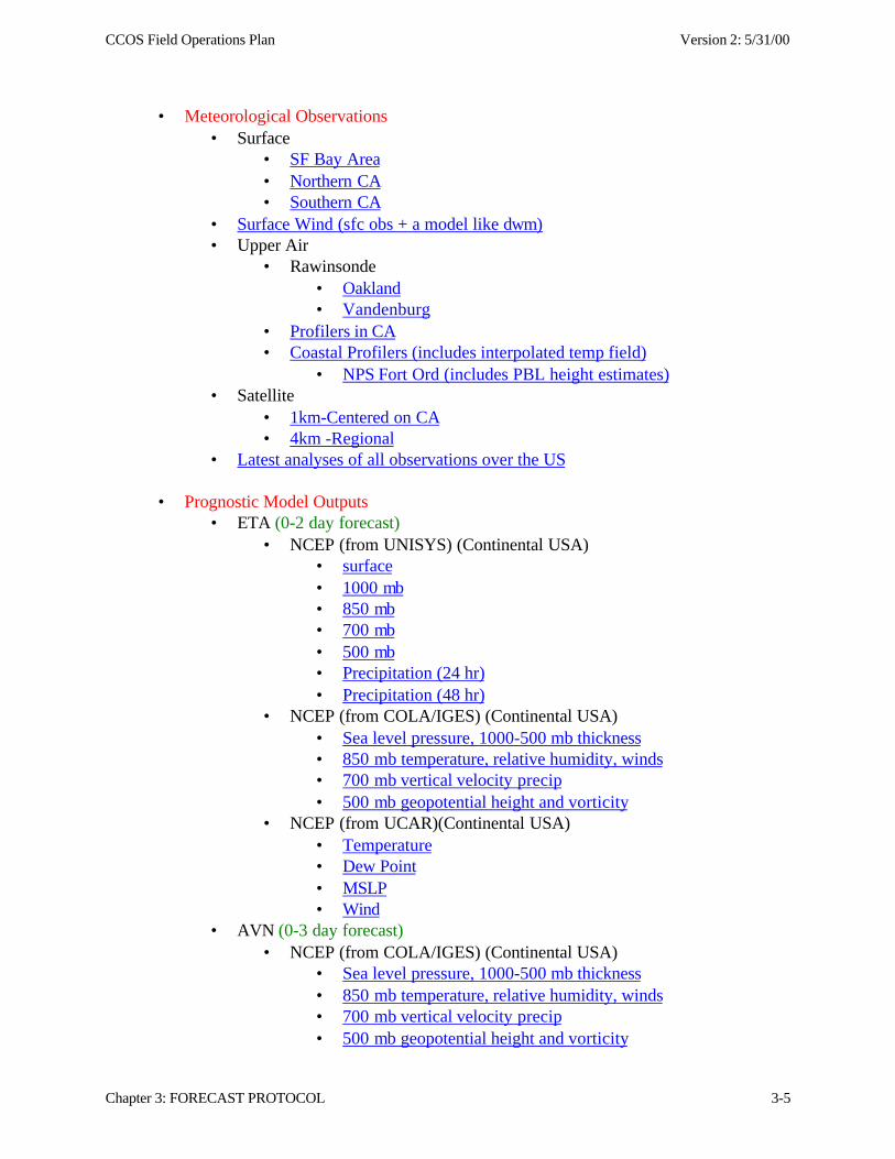
CCOS Field Operations Plan Version 2: 5/31/00
Chapter 3: FORECAST PROTOCOL 3-5
• Meteorological Observations• Surface
• SF Bay Area• Northern CA• Southern CA
• Surface Wind (sfc obs + a model like dwm)• Upper Air
• Rawinsonde• Oakland• Vandenburg
• Profilers in CA• Coastal Profilers (includes interpolated temp field)
• NPS Fort Ord (includes PBL height estimates)• Satellite
• 1km-Centered on CA• 4km -Regional
• Latest analyses of all observations over the US
• Prognostic Model Outputs• ETA (0-2 day forecast)
• NCEP (from UNISYS) (Continental USA)• surface• 1000 mb• 850 mb• 700 mb• 500 mb• Precipitation (24 hr)• Precipitation (48 hr)
• NCEP (from COLA/IGES) (Continental USA)• Sea level pressure, 1000-500 mb thickness• 850 mb temperature, relative humidity, winds• 700 mb vertical velocity precip• 500 mb geopotential height and vorticity
• NCEP (from UCAR)(Continental USA)• Temperature• Dew Point• MSLP• Wind
• AVN (0-3 day forecast)• NCEP (from COLA/IGES) (Continental USA)
• Sea level pressure, 1000-500 mb thickness• 850 mb temperature, relative humidity, winds• 700 mb vertical velocity precip• 500 mb geopotential height and vorticity
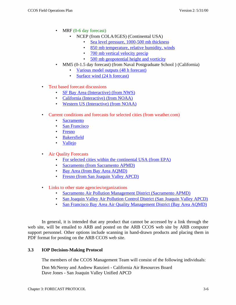
CCOS Field Operations Plan Version 2: 5/31/00
Chapter 3: FORECAST PROTOCOL 3-6
• MRF (0-6 day forecast)• NCEP (from COLA/IGES) (Continental USA)
• Sea level pressure, 1000-500 mb thickness• 850 mb temperature, relative humidity, winds• 700 mb vertical velocity precip• 500 mb geopotential height and vorticity
• MM5 (0-1.5 day forecast) (from Naval Postgraduate School ) (California)• Various model outputs (48 h forecast)• Surface wind (24 h forecast)
• Text based forecast discussions• SF Bay Area (Interactive) (from NWS)• California (Interactive) (from NOAA)• Western US (Interactive) (from NOAA)
• Current conditions and forecasts for selected cities (from weather.com)• Sacramento• San Francisco• Fresno• Bakersfield• Vallejo
• Air Quality Forecasts• For selected cities within the continental USA (from EPA)• Sacramento (from Sacramento APMD)• Bay Area (from Bay Area AQMD)• Fresno (from San Joaquin Valley APCD)
• Links to other state agencies/organizations• Sacramento Air Pollution Management District (Sacramento APMD)• San Joaquin Valley Air Pollution Control District (San Joaquin Valley APCD)• San Francisco Bay Area Air Quality Management District (Bay Area AQMD)
In general, it is intended that any product that cannot be accessed by a link through theweb site, will be emailed to ARB and posted on the ARB CCOS web site by ARB computersupport personnel. Other options include scanning in hand-drawn products and placing them inPDF format for posting on the ARB CCOS web site.
3.3 IOP Decision-Making Protocol
The members of the CCOS Management Team will consist of the following individuals:
Don McNerny and Andrew Ranzieri - California Air Resources BoardDave Jones - San Joaquin Valley Unified APCD
CCOS Field Operations Plan Version 2: 5/31/00
Chapter 3: FORECAST PROTOCOL 3-7
Rob DeMandel - San Francisco Bay Area AQMDBridget Tollstrup - Sacramento Municipal AQMD
Technical SupportSaffet Tanrikulu (ARB) – Forecast Team recommendationEric Fujita (DRI) – Operational Status and Air Quality Data/IOP history
After the forecast team reaches a consensus forecast, a recommendation will be made bythe forecast team leader to the Management Team. The go/no-go decision of the managementteam will be posted by 0300 PDT on the ARB CCOS site and pertinent information will beplaced on the voicemail of a call-in line that each CCOS field study contractor is responsible tocheck on a daily basis.
IOP decision posted at web site: http://www.arb.ca.gov/themis/forecast_iop.docIOP decision call-in line: 916/324-1953
The following criteria will be used to decide whether or not to conduct IOP sampling:
• Forecasted meteorological conditions must be favorable for formation and accumulation ofhigh ozone concentrations.
• Forecasted ozone concentrations of 125 ppb or higher, including a “ramp-up” day before thehigh-ozone day.
• Capture a minimum of one ozone episodes in each of the three major air basins within the -Bay Area, Sacramento Valley, and San Joaquin Valley. The location of the predicted highozone will have less influence on the decision to call an IOP during the first ten IOP daysthan during the last five IOPs.
• Operational readiness.
• Aircraft crews require at least one day without sampling after three consecutive days ofoperation.
A daily schedule of forecasting and decision-making is shown in Table 3.3-1. Thetimeline is roughly as follows. Since we would like to get a ramp-up day in the episode, i.e., startmeasurements one day before the high-ozone, we need a 96-hour forecast (approximately 96hours preceding the peak ozone of the episode) for the high-ozone day, permitting a 57-hour leadtime to put the sampler field crew on alert and a 63-hour lead time to put aircraft pilots on alert.Aircraft operations can be performed with a 39-hour lead time, but 63 hours are desirable for theoriginal alert status. The 24-hour forecast will also include a confirmation of a go decision,which could otherwise be canceled at if conditions change appreciable from those forecasted,permitting the sampler field crew only 9 hours to cancel the start of sampling.
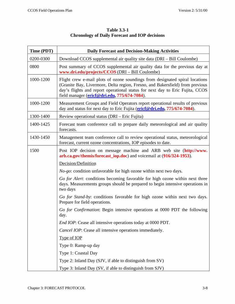
CCOS Field Operations Plan Version 2: 5/31/00
Chapter 3: FORECAST PROTOCOL 3-8
Table 3.3-1Chronology of Daily Forecast and IOP decisions
Time (PDT) Daily Forecast and Decision-Making Activities
0200-0300 Download CCOS supplemental air quality site data (DRI – Bill Coulombe)
0800 Post summary of CCOS supplemental air quality data for the previous day atwww.dri.edu/projects/CCOS (DRI – Bill Coulombe)
1000-1200 Flight crew e-mail plots of ozone soundings from designated spiral locations(Granite Bay, Livermore, Delta region, Fresno, and Bakersfield) from previousday’s flights and report operational status for next day to Eric Fujita, CCOSfield manager ([email protected], 775/674-7084).
1000-1200 Measurement Groups and Field Operators report operational results of previousday and status for next day to Eric Fujita ([email protected], 775/674-7084).
1300-1400 Review operational status (DRI – Eric Fujita)
1400-1425 Forecast team conference call to prepare daily meteorological and air qualityforecasts.
1430-1450 Management team conference call to review operational status, meteorologicalforecast, current ozone concentrations, IOP episodes to date.
1500 Post IOP decision on message machine and ARB web site (http://www.arb.ca.gov/themis/forecast_iop.doc) and voicemail at (916/324-1953).
Decision/Definition
No-go: condition unfavorable for high ozone within next two days.
Go for Alert: conditions becoming favorable for high ozone within next threedays. Measurements groups should be prepared to begin intensive operations intwo days
Go for Stand-by: conditions favorable for high ozone within next two days.Prepare for field operations.
Go for Confirmation: Begin intensive operations at 0000 PDT the followingday.
End IOP: Cease all intensive operations today at 0000 PDT.
Cancel IOP: Cease all intensive operations immediately.
Type of IOP
Type 0: Ramp-up day
Type 1: Coastal Day
Type 2: Inland Day (SJV, if able to distinguish from SV)
Type 3: Inland Day (SV, if able to distinguish from SJV)
CCOS Field Operations Plan Version 2: 5/31/00
Chapter 4: QUALITY ASSURANCE 4-1
4.0 QUALITY ASSURANCE
This section provides a summary of planned quality assurance tasks/activities for CCOSand delineates the responsibilities of the quality assurance team. The purpose of qualityassurance (QA) is to provide a quantitative estimate of the uncertainty of the measurementsthrough estimates of the precision, accuracy (or bias), and validity. In addition, QA ensures thatthe procedures and sampling methods used in the study are well documented and are capable ofproducing data that meet the specifications of the study. The QA team reviews the investigators'standard operating procedures (SOPs) and makes estimates of the precision and accuracy thatmight be expected from the measurement systems. Prior to or during sampling the QA teamcarries out quality audits and helps resolve any problems.
Quality assurance includes two types of activities: quality control (QC), and qualityauditing. The QC activities are on-going activities of the measurement and data processingpersonnel. QC activities consist of written standard operating procedures to be followed duringsample collection, sample analysis, and data processing. These procedures define schedules forperiodic calibrations and performance tests (including blank and replicate analyses). Theyspecify pre-defined tolerances that are not to be exceeded by performance tests and the actions tobe taken when they are exceeded. The QC activities also include equipment maintenance, andacceptance testing, and operator training, supervision, and support.
Quality auditing consists of two components: systems audits and performance audits.Systems audits include a review of the operational and quality control (QC) procedures to assesswhether they are adequate to assure valid data that meet the specified level of accuracy andprecision. After reviewing the procedures, the auditor examines phases of the measurement ordata processing activity to determine whether the procedures are being followed and that theoperating personnel are properly trained. The system audit is a cooperative assessment resultingin improved data. Performance audits establish whether the predetermined specifications foraccuracy are being achieved in practice.
Performance audit involves challenging the measurement/analysis system with a knownstandard sample that is traceable to a primary standard. Precision is quantified by periodicallychallenging a measurement device with known, identical input conditions. In evaluatingprecision and accuracy objectives, it is important to consider the methods used to determine thevalues. For example, a greater deviation may occur between replicates with real samples withcomplex matrices than with replicates of standards in simple matrices. Synthetic mixtures ofhydrocarbons that are used in the Photochemical Assessment Monitoring Station Program forlaboratory intercomparisons and through-the-probe audits are examples. An ambient sampleyields a more complex chromatogram and greater potential for inconsistent identification.Analysis of a standard mixture of hydrazones does not address potential sampling artifacts thatmay be associated with carbonyl compound measurements using the DNPH derivitizationmethod. Measurement intercomparisons are used to assess the representativeness, accuracy, andprecision of measurements that preclude standard performance audits (e.g., PAN, NOy, ozonelidar, upper air meteorology).
CCOS Field Operations Plan Version 2: 5/31/00
Chapter 4: QUALITY ASSURANCE 4-2
4.1 Quality Assurance Organization, Responsibilities, and Tasks
Quality assurance will be under the overall direction of the CCOS QA manager, Mr.David Bush of Parsons Engineering Science. He is also the QA manager for CRPAQS, and isconsequently already managing the external quality assurance efforts for many existingmeasurement efforts that will ultimately be part of the CCOS database. Due to the scope of theCCOS supplemental monitoring effort, Parsons has assembled a QA management team tospecifically address the many aspects of the monitoring program. Mr. Robert Baxter (Parsons)will be responsible for overseeing the audits of the surface and upper air meteorologicalmeasurements. He will be responsible for coordinating the meteorological audits, interfacingwith supporting subcontractors (Northwest Research Associates, Inc. and T&B Systems), andreviewing all data and reports associated with the meteorological audits. Much of the informationin this section is a summary of the December 1999 proposal written by Parsons EngineeringScience. The QA manager will also coordinate with QA staffs from the California Air ResourcesBoard (Mr. Michael Miguel) and the Bay Area AQMD (Mr. Avi Okin). ARB and BAAQMDwill conduct performance audits of the ozone, NO/NOx, NO/NOy analyzers at exitingmonitoring stations and at CCOS supplemental monitoring sites within their area ofresponsibility.
The principle objective of the CCOS QA program is to ensure that the established dataquality objectives (DQOs) are achieved. The overall responsibility of QA manager will be toinform the CCOS Program Manager and the CCOS Technical Committee of the steps beingtaken to control and quantify data quality, provide guidance to the study participants in carryingout their quality assurance responsibilities, and to provide a framework for using quality controltest data to create data qualification statements for the data archive. The responsibilities of theCCOS QA manager include the following tasks.
Task 1: Evaluate sampling and analysis methods, and review system and performanceaudit procedures. The QA team will request from each CCOS measurement contractor a qualityintegrated work plan (QIWP), which covers all aspects of their work, as well as standardoperating procedures (SOPs) for each specific operation. The QIWP and SOPs describe theapproach for maintaining and quantifying data quality for each measurement, and will includedescriptions of and specifications for calibration, standards, control limits, data processing, andother data quality related topics. As part of this effort, the QA team will provide guidance tomeasurement contractors in preparing the QIWP, using the QIWP guidance document previouslyprepared for CRPAQS. The QA team will review the data quality objectives in the QIWPs andverify the assumptions on which the measurements are based, and determine whether themethods are likely to meet the specifications for accuracy (or bias) and precision.Recommendations for revisions to the QIWPs and SOPs will be submitted to the measurementcontractors. Once QIWPs and SOPs have been finalized, they will be submited to the CCOSdata manager for the data archive.
Task 2: Prepare a quality assurance plan for CCOS. The QA manager will develop aquality assurance plan in conjunction with the CCOS field manager, field contractors, and QApersonnel from the Districts and ARB. The plan will use the NARSTO-formatted ProgramQuality Management Plan (PQMP) developed for CRPAQS as a basis. The plan will includedata quality objectives, descriptions of quality control procedures for each measurement group,
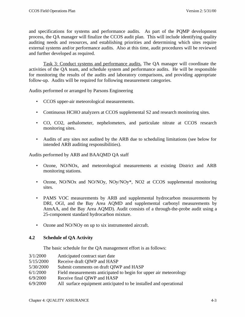
CCOS Field Operations Plan Version 2: 5/31/00
Chapter 4: QUALITY ASSURANCE 4-3
and specifications for systems and performance audits. As part of the PQMP developmentprocess, the QA manager will finalize the CCOS audit plan. This will include identifying qualityauditing needs and resources, and establishing priorities and determining which sites requireexternal systems and/or performance audits. Also at this time, audit procedures will be reviewedand further developed as required.
Task 3: Conduct systems and performance audits. The QA manager will coordinate theactivities of the QA team, and schedule system and performance audits. He will be responsiblefor monitoring the results of the audits and laboratory comparisons, and providing appropriatefollow-up. Audits will be required for following measurement categories.
Audits performed or arranged by Parsons Engineering
• CCOS upper-air meteorological measurements.
• Continuous HCHO analyzers at CCOS supplemental S2 and research monitoring sites.
• CO, CO2, aethalometer, nephelometers, and particulate nitrate at CCOS researchmonitoring sites.
• Audits of any sites not audited by the ARB due to scheduling limitations (see below forintended ARB auditing responsibilities).
Audits performed by ARB and BAAQMD QA staff
• Ozone, NO/NOx, and meteorological measurements at existing District and ARBmonitoring stations.
• Ozone, NO/NOx and NO/NOy, NOy/NOy*, NO2 at CCOS supplemental monitoringsites.
• PAMS VOC measurements by ARB and supplemental hydrocarbon measurements byDRI, OGI, and the Bay Area AQMD and supplemental carbonyl measurements byAtmAA, and the Bay Area AQMD). Audit consists of a through-the-probe audit using a25-component standard hydrocarbon mixture.
• Ozone and NO/NOy on up to six instrumented aircraft.
4.2 Schedule of QA Activity
The basic schedule for the QA management effort is as follows:
3/1/2000 Anticipated contract start date5/15/2000 Receive draft QIWP and HASP5/30/2000 Submit comments on draft QIWP and HASP6/1/2000 Field measurements anticipated to begin for upper air meteorology6/9/2000 Receive final QIWP and HASP6/9/2000 All surface equipment anticipated to be installed and operational
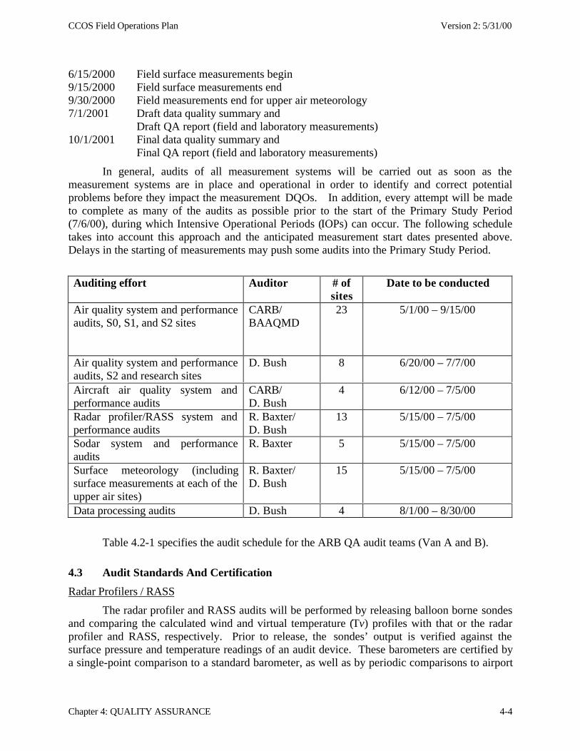
CCOS Field Operations Plan Version 2: 5/31/00
Chapter 4: QUALITY ASSURANCE 4-4
6/15/2000 Field surface measurements begin9/15/2000 Field surface measurements end9/30/2000 Field measurements end for upper air meteorology7/1/2001 Draft data quality summary and
Draft QA report (field and laboratory measurements)10/1/2001 Final data quality summary and
Final QA report (field and laboratory measurements)
In general, audits of all measurement systems will be carried out as soon as themeasurement systems are in place and operational in order to identify and correct potentialproblems before they impact the measurement DQOs. In addition, every attempt will be madeto complete as many of the audits as possible prior to the start of the Primary Study Period(7/6/00), during which Intensive Operational Periods (IOPs) can occur. The following scheduletakes into account this approach and the anticipated measurement start dates presented above.Delays in the starting of measurements may push some audits into the Primary Study Period.
Auditing effort Auditor # ofsites
Date to be conducted
Air quality system and performanceaudits, S0, S1, and S2 sites
CARB/BAAQMD
23 5/1/00 – 9/15/00
Air quality system and performanceaudits, S2 and research sites
D. Bush 8 6/20/00 – 7/7/00
Aircraft air quality system andperformance audits
CARB/D. Bush
4 6/12/00 – 7/5/00
Radar profiler/RASS system andperformance audits
R. Baxter/D. Bush
13 5/15/00 – 7/5/00
Sodar system and performanceaudits
R. Baxter 5 5/15/00 – 7/5/00
Surface meteorology (includingsurface measurements at each of theupper air sites)
R. Baxter/D. Bush
15 5/15/00 – 7/5/00
Data processing audits D. Bush 4 8/1/00 – 8/30/00
Table 4.2-1 specifies the audit schedule for the ARB QA audit teams (Van A and B).
4.3 Audit Standards And Certification
Radar Profilers / RASS
The radar profiler and RASS audits will be performed by releasing balloon borne sondesand comparing the calculated wind and virtual temperature (Tv) profiles with that or the radarprofiler and RASS, respectively. Prior to release, the sondes’ output is verified against thesurface pressure and temperature readings of an audit device. These barometers are certified bya single-point comparison to a standard barometer, as well as by periodic comparisons to airport
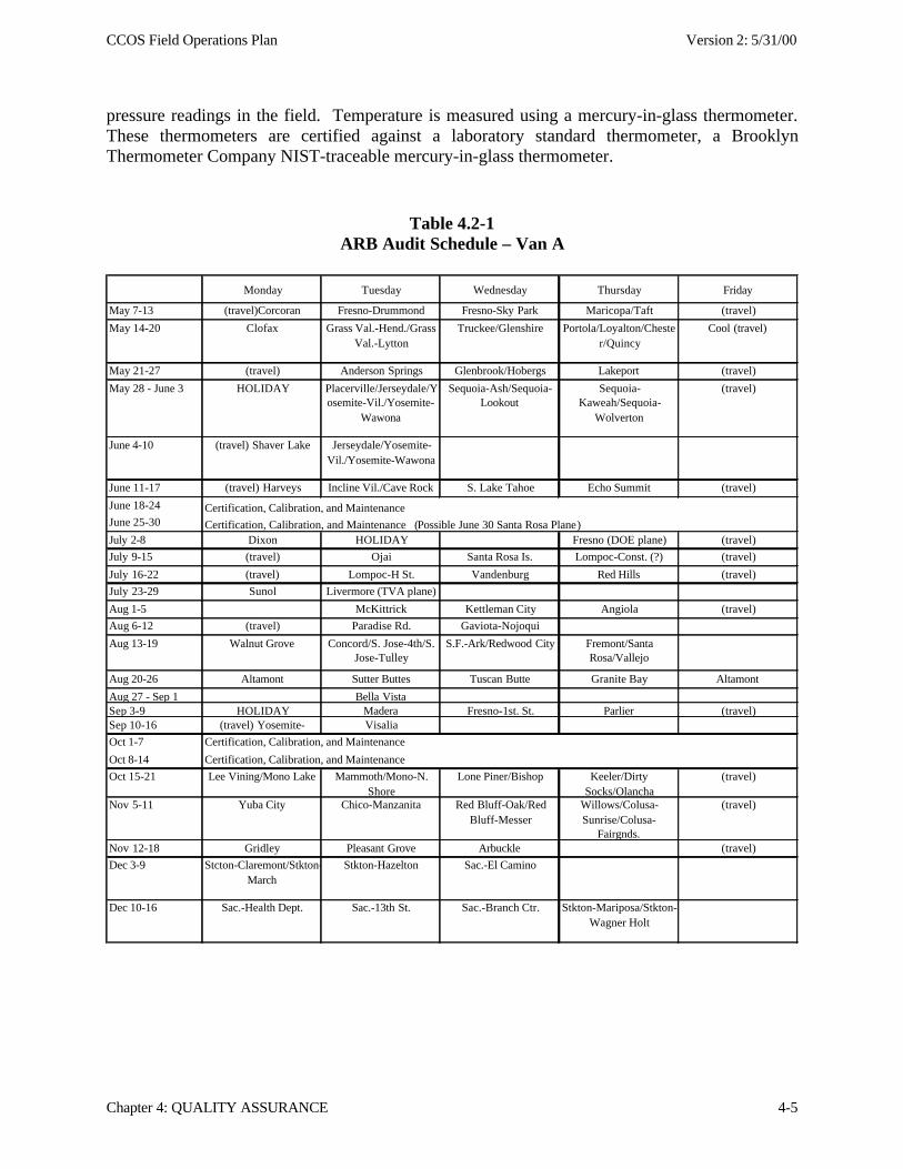
CCOS Field Operations Plan Version 2: 5/31/00
Chapter 4: QUALITY ASSURANCE 4-5
pressure readings in the field. Temperature is measured using a mercury-in-glass thermometer.These thermometers are certified against a laboratory standard thermometer, a BrooklynThermometer Company NIST-traceable mercury-in-glass thermometer.
Table 4.2-1ARB Audit Schedule – Van A
Monday Tuesday Wednesday Thursday Friday
May 7-13 (travel)Corcoran Fresno-Drummond Fresno-Sky Park Maricopa/Taft (travel)
May 14-20 Clofax Grass Val.-Hend./Grass Val.-Lytton
Truckee/Glenshire Portola/Loyalton/Chester/Quincy
Cool (travel)
May 21-27 (travel) Anderson Springs Glenbrook/Hobergs Lakeport (travel)
May 28 - June 3 HOLIDAY Placerville/Jerseydale/Yosemite-Vil./Yosemite-
Wawona
Sequoia-Ash/Sequoia-Lookout
Sequoia-Kaweah/Sequoia-
Wolverton
(travel)
June 4-10 (travel) Shaver Lake Jerseydale/Yosemite-Vil./Yosemite-Wawona
June 11-17 (travel) Harveys Incline Vil./Cave Rock S. Lake Tahoe Echo Summit (travel)
June 18-24 Certification, Calibration, and MaintenanceJune 25-30 Certification, Calibration, and Maintenance (Possible June 30 Santa Rosa Plane)July 2-8 Dixon HOLIDAY Fresno (DOE plane) (travel)
July 9-15 (travel) Ojai Santa Rosa Is. Lompoc-Const. (?) (travel)
July 16-22 (travel) Lompoc-H St. Vandenburg Red Hills (travel)
July 23-29 Sunol Livermore (TVA plane)
Aug 1-5 McKittrick Kettleman City Angiola (travel)
Aug 6-12 (travel) Paradise Rd. Gaviota-Nojoqui
Aug 13-19 Walnut Grove Concord/S. Jose-4th/S. Jose-Tulley
S.F.-Ark/Redwood City Fremont/Santa Rosa/Vallejo
Aug 20-26 Altamont Sutter Buttes Tuscan Butte Granite Bay Altamont
Aug 27 - Sep 1 Bella VistaSep 3-9 HOLIDAY Madera Fresno-1st. St. Parlier (travel)Sep 10-16 (travel) Yosemite-
TurtlebackVisalia
Oct 1-7 Certification, Calibration, and Maintenance
Oct 8-14 Certification, Calibration, and Maintenance
Oct 15-21 Lee Vining/Mono Lake Mammoth/Mono-N. Shore
Lone Piner/Bishop Keeler/Dirty Socks/Olancha
(travel)
Nov 5-11 Yuba City Chico-Manzanita Red Bluff-Oak/Red Bluff-Messer
Willows/Colusa-Sunrise/Colusa-
Fairgnds.
(travel)
Nov 12-18 Gridley Pleasant Grove Arbuckle (travel)
Dec 3-9 Stcton-Claremont/Stkton-March
Stkton-Hazelton Sac.-El Camino
Dec 10-16 Sac.-Health Dept. Sac.-13th St. Sac.-Branch Ctr. Stkton-Mariposa/Stkton-Wagner Holt
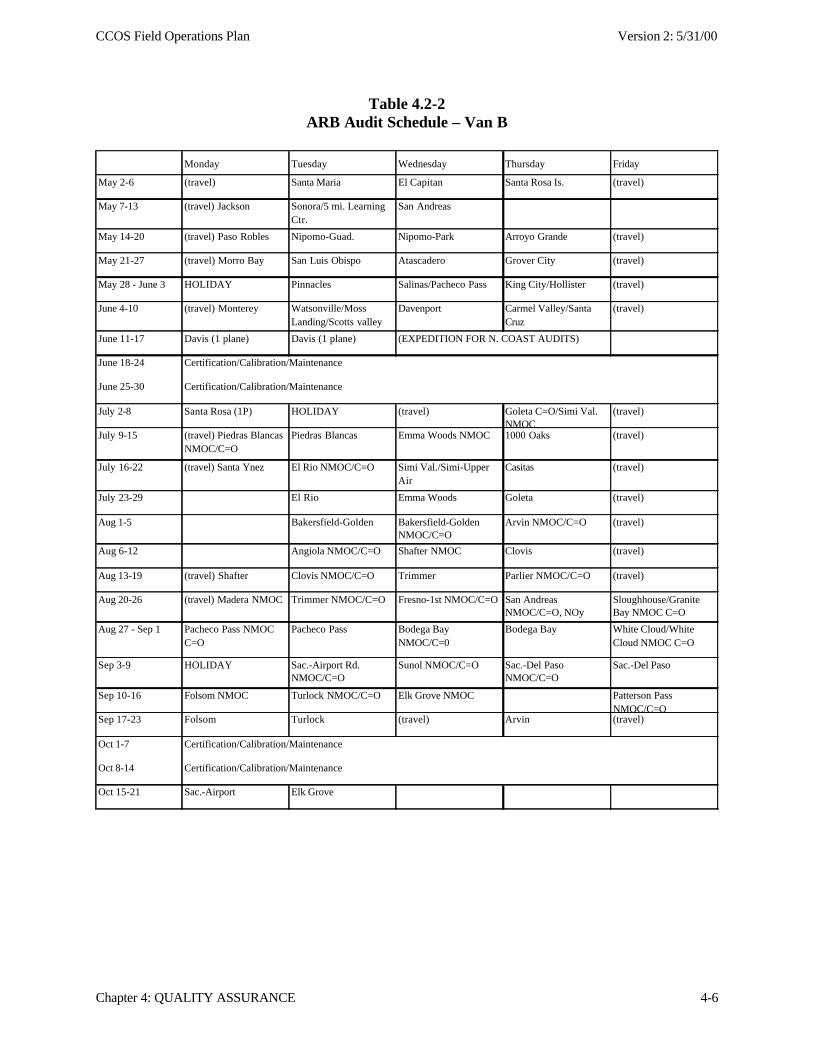
CCOS Field Operations Plan Version 2: 5/31/00
Chapter 4: QUALITY ASSURANCE 4-6
Table 4.2-2ARB Audit Schedule – Van B
Monday Tuesday Wednesday Thursday Friday
May 2-6 (travel) Santa Maria El Capitan Santa Rosa Is. (travel)
May 7-13 (travel) Jackson Sonora/5 mi. Learning Ctr.
San Andreas
May 14-20 (travel) Paso Robles Nipomo-Guad. Nipomo-Park Arroyo Grande (travel)
May 21-27 (travel) Morro Bay San Luis Obispo Atascadero Grover City (travel)
May 28 - June 3 HOLIDAY Pinnacles Salinas/Pacheco Pass King City/Hollister (travel)
June 4-10 (travel) Monterey Watsonville/Moss Landing/Scotts valley
Davenport Carmel Valley/Santa Cruz
(travel)
June 11-17 Davis (1 plane) Davis (1 plane) (EXPEDITION FOR N. COAST AUDITS)
June 18-24 Certification/Calibration/Maintenance
June 25-30 Certification/Calibration/Maintenance
July 2-8 Santa Rosa (1P) HOLIDAY (travel) Goleta C=O/Simi Val. NMOC
(travel)
July 9-15 (travel) Piedras Blancas NMOC/C=O
Piedras Blancas Emma Woods NMOC 1000 Oaks (travel)
July 16-22 (travel) Santa Ynez El Rio NMOC/C=O Simi Val./Simi-Upper Air
Casitas (travel)
July 23-29 El Rio Emma Woods Goleta (travel)
Aug 1-5 Bakersfield-Golden Bakersfield-Golden NMOC/C=O
Arvin NMOC/C=O (travel)
Aug 6-12 Angiola NMOC/C=O Shafter NMOC Clovis (travel)
Aug 13-19 (travel) Shafter Clovis NMOC/C=O Trimmer Parlier NMOC/C=O (travel)
Aug 20-26 (travel) Madera NMOC Trimmer NMOC/C=O Fresno-1st NMOC/C=O San Andreas NMOC/C=O, NOy
Sloughhouse/Granite Bay NMOC C=O
Aug 27 - Sep 1 Pacheco Pass NMOC C=O
Pacheco Pass Bodega Bay NMOC/C=0
Bodega Bay White Cloud/White Cloud NMOC C=O
Sep 3-9 HOLIDAY Sac.-Airport Rd. NMOC/C=O
Sunol NMOC/C=O Sac.-Del Paso NMOC/C=O
Sac.-Del Paso
Sep 10-16 Folsom NMOC Turlock NMOC/C=O Elk Grove NMOC Patterson Pass NMOC/C=O
Sep 17-23 Folsom Turlock (travel) Arvin (travel)
Oct 1-7 Certification/Calibration/Maintenance
Oct 8-14 Certification/Calibration/Maintenance
Oct 15-21 Sac.-Airport Elk Grove
CCOS Field Operations Plan Version 2: 5/31/00
Chapter 4: QUALITY ASSURANCE 4-7
Surface Meteorology
Wind Speed - Anemometer Drive. An R.M.Young Model 18801 anemometer drive iscertified quarterly. A photo tachometer is used to determine the actual rotational speed of theanemometer drive shaft for comparison with the rotational speed indicated by the anemometerdrive display. Readings are made at six speeds evenly spaced through the entire operating rangeof the instrument. Additionally, the frequency output from the drive is verified against a digitalfrequency counter. Torque Disk (no certification required).
Wind Direction - Compass (no certification required). Torque Disk (no certificationrequired).
Ambient Temperature - Mercury-in-glass thermometer. Audit mercury-in-glassthermometers are compared to an NIST-traceable standard thermometer when they arepurchased. The two thermometers were immersed in water baths of approximately zero, 10°,20°, 30° and 40°C. Periodic comparisons with the standard thermometer are not required if theoperating ranges of the thermometers are not exceeded.
Relative Humidity and Dew-point Temperature – Psychrometer mercury-in-glassthermometers. The psychrometer mercury-in-glass thermometers are compared to an NIST-traceable standard thermometer when purchased. The two psychrometer thermometers and thestandard thermometer were immersed in water baths of approximately zero, 10°, 20°, 30° and40°C. Periodic comparisons with the standard thermometer are not required if the operatingranges of the thermometers are not exceeded.
Pressure - Audit barometer (Peet Brothers Ultimeter Model 3). The audit barometer iscompared with a standard barometer on a yearly basis.
Total Solar Radiation – Pyranometer. Audit pyranometers are checked annually bycomparing the pyranometers output with an independent pyranometer maintained by AVES’sQA group. The voltmeter is used to read the audit pyranometer outputs is certified on an annualbasis.
Rawinsondes. Audit barometer (Peet Brothers Ultimeter Model 3). The audit barometer iscompared on a regular basis with a standard barometer maintained by AVES. The psychrometermercury-in-glass thermometers are compared to an NIST-traceable standard thermometer whenpurchased. The two psychrometer thermometers and the standard thermometer were immersedin water baths of approximately zero, 10°, 20°, 30° and 40°C. Periodic comparisons with thestandard thermometer are not required if the operating ranges of the thermometers are notexceeded.
Flow Measurements.
QA Standards - All flow meters used for the field audits will be compared against flowstandards maintained by AVES/ATC Associaates at its QA laboratory in Monrovia, California,or against similar flow standards. These standards are used to certify the flow transfer standardsthat are used in the field. AVES’s QA flow standards are summarized below:

CCOS Field Operations Plan Version 2: 5/31/00
Chapter 4: QUALITY ASSURANCE 4-8
Device Manufacturer Model Element Range
Bubble meter Teledyne/Hastings 0 - 5 lpmLaminar flow meter Meriam 50MK10 725250-C1 0 - 50 cc/minLaminar flow meter Meriam 50MK10 725250-C2 0 - 1 lpmLaminar flow meter Meriam 50MJ10-1/2 700310-T2 0 - 10 lpmLaminar flow meter Meriam 50MJ10-1/2 700310-T1 0 - 50 lpmLaminar flow meter Meriam 50MW20-1 700310-T3 0 - 200 lpm
The Laminar flow devices are certified annually against a primary flow standard by an externallaboratory. The bubble flow meter is a primary flow measuring device, and therefore requires nocertification. Parsons also maintains a bubble flow meter.
Flow Meters - Several flow meters are available as transfer standards for this study.These flow meters and their operating ranges are summarized below:
Make Model SN Range TypeBubble-O 0 - 400 ccpm BubbleBios DC-Lite 0 - 20 lpm PistonSchlumberger Remus 4, G1-6 0 - 20 lpm Dry testTeledyne-Hastings HS-10KS 16045 0 - 10 lpm Mass flowTeledyne-Hastings HS-50JS 16944 0 - 50 lpm Mass flowTeledyne-Hastings HS-10S 17259 0 - 150 lpm Mass flow
All flow meters will be certified against suitable flow standards prior to being used in the field.Certifications consist of a comparison between the flow meter and the appropriate QA laminarflow standard at at least 10 different flow spaced evenly across the operating range of the massflow meter.
Continuous Air Quality Analyzers
Dilution Standards and Gases - Multipoint audits will be performed using either a Dasibi1009 CP dilution system, an Environics Series 100 dilution system, or equivalent system. Thesesystems are maintained and the flow rates certified by Parsons’ and the departments. The zero air source will be either a cylinder of Ultra-Pure Air that will be suppliedby Scott Specialty Gases or an Aadco 737R pure air system with CH4 burner and compressorcapable of delivering a constant 20 lpm air supply. The span gases, except for the SUVArefrigerant, will be provided by Scott Specialty Gases. All gas standard analysis is performed inaccordance with EPA Protocols and is traceable to National Institute of Standards andTechnology (NIST) standards.) For the CCOS audits, Relative Accuracy Test Audits (RATA)Class cylinders will be used, which are certified to with ±1% of true. SUVA refrigerant will beused to audit the nephelometers. This compound has a known scattering coefficient that iswithin the nephelometer measurement range.
Ozone - All field ozone transfer standards will be certified against a primary standard.Procedures for certification and recertification of ozone primary and transfer standards are basedon the EPA technical assistance document, Transfer Standards for Calibration of Air MonitoringAnalyzers for Ozone (EPA 1979), EPA-600/4-79-056. All ozone transfer standards used for
CCOS Field Operations Plan Version 2: 5/31/00
Chapter 4: QUALITY ASSURANCE 4-9
CCOS will be compared against the California ARB standard photometer prior to the audits.The ozone transfer standards used for CCOS will be an API 400, a Dasibi 5009 MC or a Dasibi1003 PC ozone analyzer. These ozone analyzers have been converted to a transfer standardconfiguration in accordance with EPA guidelines (September, 1979). Ozone analyzers that areconverted to a transfer standard configuration must be compared to a primary ozone standard bymeans of a 6 x 6 comparison as the final step in the conversion process. Ozone transferstandards that are in regular use must be compared by means of a 1 x 6 (zero and five upscaleconcentration points) comparison with the a primary ozone standard twice per quarter.
NMOC/carbonyl samplers
Laboratory performance audits of the analytical methods for non-methane organichydrocarbons (NMOCs) and carbonyls will be conducted to assess the accuracy of the methodsused by the laboratory to measure the ambient concentrations, as well as the sampling systems.Audits are conducted by supplying the laboratory with a cylinder containing a mixture of targetorganic hydrocarbons and carbonyl standards prepared by the National Institute of Standards andTechnology (NIST). The laboratory analyzes the contents of the cylinder following their normalstandard operating procedures.
4.4 System Audit Procedures
4.4.1 Radar Profilers and RASS
The system audit of the radar profiler begins with an inspection of the antenna andcontroller interface cables for proper connection. Antennas and enclosures or clutter fences areinspected for structural integrity. The orientation of the antennas are checked using a magnetictransit and tripod with the observed magnetic readings corrected to true directions using the localmagnetic declination. The magnetic orientation measurements are also verified using solarazimuth measurements and latitude and longitude information obtained from handheld GPS.The inclinations of the antennas are measured using a Pro SMARTLEVEL. Measurements aremade in at least two directions on the bottom of the antenna array’s support structure. For themultiple antenna systems the inclination angle is also measured and compared to the softwaresetting.
A vista diagram is prepared that documents the surroundings of the site. The diagramidentifies potential reflective sources for the radar signal, as well as potential active sources thatcould generate interference. The diagram also provides a description of the view in 30-degreeincrements around the antenna, including the elevation angle and estimated distance to potentialsources.
If the configuration of the system allows, an evaluation of the total noise spectrum isperformed with the system "listening only," i.e., without transmitting a pulse. The results of thischeck should produce no measured winds or temperature, or data with very low reliability. Ifreliable data points are reported at any level, then there is probably an active noise source in thearea that is generating frequencies in the operational region of the radar or RASS.
CCOS Field Operations Plan Version 2: 5/31/00
Chapter 4: QUALITY ASSURANCE 4-10
A scan of frequencies around the central operating frequency of the radar is performedusing an RF scanner. This method has been successfully used in past RWP audits to confirm useof adjacent frequencies by nearby communication operations and to identify the sources of activenoise contaminating the wind and virtual temperature data.
The settings of the controller and data collection devices are checked and noted to ensurethat the instrument is operating in the proper mode and that the data being collected are thosespecified by the SOPs. This includes a check of all clocks for accuracy, verifying that they arewithin ±2 minutes of the standard. The site operator is interviewed to determine his/herknowledge of the system operation, maintenance and proficiency in the performance of QCchecks. Emphasis is placed on verifying that preventive maintenance procedures have beenimplemented and are adequate. The station logbooks are reviewed for completeness and content.Finally, data collected over several days are reviewed for reasonableness and consistency.
An orientation accuracy criterion of ±2° will be used. For level and inclination angle ofoblique antennas we will use ±0.5°. The overall procedures are consistent with recent EPAguidance (EPA 1999).
4.4.2 Sodars
The sodar system audit is divided into several tasks. A description of each task isprovided below:
An evaluation of the site characteristics is performed. Passive and active noise sourcesare identified and noted to evaluate their impact on the sodar's ability to separate the returnpulses from the background noise. Passive sources are objects that may reflect the pulse andcontaminate the return spectra with what appears to be near-zero wind speeds. These sourcesinclude buildings, trees, nearby towers, etc. Active sources generate their own noise such as airconditioners, fans and industrial complexes. Low-level active white noise sources are notgenerally a problem except to reduce the maximum altitude. Active noise sources in thefrequency spectrum of the sodar operations may affect the operations. General sound levels aremeasured using an integrating sound level meter and measuring levels, in dBA, in at least thefour cardinal directions. A spectral analysis of the background noise is performed to determine ifthere are significant sources within the operating range of the sodar.
In addition to the evaluation of the total noise spectrum above, a system check isperformed with the system "listening only," i.e., without transmitting a pulse. The results of thischeck should produce no measured winds, or winds with very low reliability. If reliable windsare reported at any level, then there is probably an active noise source in the area that isgenerating frequencies in the operational region of the sodar.
A vista diagram is prepared that documents the surroundings of the site. The diagramidentifies potential reflective sources for the radar signal, as well as potential active sources thatcould generate interference. The diagram also provides a description of the view in 30-degreeincrements around the antenna, including the elevation angle and estimated distance to potentialsources.
CCOS Field Operations Plan Version 2: 5/31/00
Chapter 4: QUALITY ASSURANCE 4-11
Alignment checks are performed on the sodar systems. The orientation of the antennaarray or individual component antennas will directly affect the accuracy of the calculated winddirections. The orientation of the respective antenna arrays is checked using a tripod mountedBrunton Pocket Transit. The measured orientation is then compared to the software settings inthe sodar. The criterion for acceptable orientation is ±2°. During the field audit, the compassalignment to magnetic north is compared against solar observations and the magnetic declinationto verify the accuracy of the magnetic measurements.
The level of a phased sodar antenna array, or inclination angle of the horizontalcomponent antennas directly affects the calculations of the component speeds. The array level(or inclination angle) is checked using a Pro SMARTLEVEL. The criterion for acceptable level(or angles) in any direction is ±0.5°, consistent with EPA (1999).
4.4.3 Surface Meteorological Measurements
The system audits of the surface meteorological sensing systems consist of an inspectionof the site to assess proper siting of the instrument sensors, a review of the station check logs andother site documentation, as well as an interview with the site operator concerning his or herknowledge of the QIWP and applicable SOP sections. Sensor siting criteria for meteorologicalsensors are specified in the EPA Quality Assurance Handbooks for Air Pollution MeasurementSystems, Volume IV (EPA, 1995). On-site forms and site logs are reviewed to check that thedocumentation conforms to the specifications of the plan. The subjects that are addressed by thesystem audits include:
Network design and siting• network size and design• sensor exposure• review of station
Resources and facilities• instruments and methods• staff and facilities• standards and traceability
Quality assurance and quality control• status of quality assurance program• audit participation• precision and accuracy checks
Additionally, once the system audits of all sites are complete, the auditor checks forpossible differences in operation among the various sites.
4.4.4 Rawinsondes
The system audits of the rawinsonde operations consist of watching a launch andcomparing the procedures used to those specified in the SOP. Special attention is paid to groundstation and sonde initialization procedures, balloon inflation (with regard to proper accent rate),
CCOS Field Operations Plan Version 2: 5/31/00
Chapter 4: QUALITY ASSURANCE 4-12
data acquisition, and flight termination. A rawinsonde system audit checklist is used during thesystem audit to ensure that all aspects of the audit are covered in a consistent manner.
4.4.5 NMOC/Carbonyl Samplers
The system audit of the NMOC/Carbonyl samplers consists of a review of the samplersiting and observation of sample loading and handling procedures. This includes observing thesite technician during routine loading and unloading of the sampler to assure that proceduresdocumented in the sampler’s SOP’s are being followed. The system audit verifies, at aminimum, the following:
• Sample chain-of-custody• Sample labeling• Sample loading procedures• Sample storage• Sample shipping procedures• Sample blanks• Flow calibration and measurement procedures• Training received by the technician• Sampler location• Pump venting• Presence of any obstructions or trees• Sampler preventive maintenance and spare parts inventory• Cyclone or impactor cleaning (if used)
A detailed system audit checklist is used during the system audit to assist the auditor anddocument the results. In general, system audit results are compared with existing EPA siting andsample handling guidelines for these samplers.
4.4.6 Continuous Gas/Particulate Analyzers
The system audits of the continuous gas/particulate analyzers, including particle countersand nephelometers, will incorporate review of the following:
• Probe height• Probe exposure• Proximity of sources• Sample manifold and/or sampling line construction• Sample residence time• Calibration procedures• Calibration standards and their certification• Zero/span checks• Preventive maintenance• Spare parts inventory• Data acquisition equipment and procedures
CCOS Field Operations Plan Version 2: 5/31/00
Chapter 4: QUALITY ASSURANCE 4-13
• Data chain-of-custody• QC documentation (site logs, checklists, etc..)• Support equipment, including station condition• Training
Preparation and handling of the solutions used to calibrate the continuous analyzers willalso be checked.
4.4.7 Additional Samplers and Analyzers
Specific audit procedures for specialized, research instrumentation will be developed asSOPs are received. This includes instrumentation such as automated VOC analyzers, HCHOdihydorlutinine derivative/fluorescent detection analyzers, TDLAS analyzers, and hydroxylcarbonyl samplers.
4.4.8 Data Processing/Management
Organizations’ data processing audits will be conducted following a data processingchecklist. The data processing audits will begin with a review of the chain-of-custodyprocedures used by each organization. The audit will examine the policies and procedures forlogging in the field data, and the maintenance and archival of all data records. The audit willexamine the procedures used to document the completeness and adequacy of the field data usedin data processing and validation. The audit will also document the sites and parametersprocessed by the organization, and the personnel who perform the data acquisition, processingand validation. All members of the organizations’ staff who perform data processing tasks willbe personally interviewed by the auditor to ensure their familiarity with all aspects of their jobs.
The audit will also document all aspects of data acquisition. This will include: (1) areview of the data logger type, (2) who is responsible for the data logger initialization, (3) thescan rate, (4) the averaging time, and (5) the averaging method. The method of electronic datacollection will also be confirmed. The audit will determine if the monitoring site is accessed bymodem, whether the modems incorporate data correction protocols, the frequency of datapolling, methods of verifying the data poll, the loading of the polled data into a data base, and theability of the site data logger to store data for extended periods in case of telecommunicationsproblems. The existence of backup strip charts will also be documented during the audit. Theaccuracy of the strip charts will be determined and the procedures for data recovery from stripcharts will be examined.
The data processing and validation procedures of each organization will be reviewed indetail by the auditor. The control limits for the air quality parameters will be documented duringeach audit, and the frequency of instrument QC checks will be confirmed. Air quality analyzerReference or Equivalent designations are frequently based upon defined station temperaturelimits. The audit will determine if the organization confirms that air quality data are collectedwithin this temperature range, and how the organization handles the data validation during timeswhere the shelter temperature was outside of this range.
CCOS Field Operations Plan Version 2: 5/31/00
Chapter 4: QUALITY ASSURANCE 4-14
The audit will examine the adequacy of field data such as station logs and checklists, andwill determine how these are used in the data processing and validation procedures of eachorganization. The audit will check the organizations procedures designed to perform anomalyscreening of the data. The audit will also confirm all steps taken to verify the accuracy of thepolled data, and determine if the digital data are confirmed using the backup strip charts (and ifso, what acceptance tolerance is defined).
The standard operating procedures of each organization will be reviewed with the dataprocessing staff during the audit. Special attention will be paid to the decision-making chain-of-command of each organization. The chain-of-command will be discussed and confirmed forroutine data processing and validation as well as for cases where problems are encountered. Theresolution of problems by the data processing staff will be confirmed during the audit. The auditwill also document the procedures used for data editing.
The data processing audits will also document the data management procedures of eachorganization. This includes confirming the data base structure and the proper entry of site,parameter, unit, and reporting precision codes by each organization. The audit will alsodetermine the existence and adequacy of data backup procedures used by each organization.
4.4.9 Laboratories
The system audits of the organization laboratories will begin with the review of theQIWPs and SOPs. Comments from those reviews will serve to ensure that analyses areappropriate to achieve the stated program goals and that the laboratory QA programs andprocedures are consistent with the selected analyses. The second step will be for the laboratoryauditor to travel to each of the organization's laboratories. The system audits in this phase willconsist of a detailed inspection of each of the organization's laboratory facilities along with anevaluation of the following program components, in accordance with the respective QIWP:sample logging, storage and identification methods; calibration procedures; preparation andstorage of standards; quality control checks (such as blanks and duplicates); chain-of-custodyprotocols; data reduction, validation and reporting methods; and the documentation of allpertinent actions.
Systems audits will be similar for each of the three laboratories. A systems audit willprovide qualitative evaluation of the overall operations of the laboratory. Emphasis is given toconfirming that all project quality control (QC) procedures are preformed and that acceptancecriteria are met. Preventive maintenance will be evaluated as well as corrective actionprocedures. Data traceably will be verified by randomly selecting a reported value and workingback through intermediate calculations and supporting paper work to the raw values. This checkconfirms error free calculation and ensures that supporting documentation is present.
Also included in the system audits will be interviews of all laboratory staff working onthe project. The interviews will focus on the staff’s familiarity with the job(s) they areperforming for the project, how they track samples and assurance of data quality and to whomthey report problems when a parameter or system is outside of the control limits.
CCOS Field Operations Plan Version 2: 5/31/00
Chapter 4: QUALITY ASSURANCE 4-15
4.5 PERFORMANCE AUDIT PROCEDURES
4.5.1 Radar Profilers
Two sets of performance audit procedures will be used that are specific to given sites. Ifthe site is equipped with a collocated sodar, the profiling system will be audited by firstestablishing the on-site sodar as an audit device and then using the sodar data collected to auditthe radar profiler data. Sites with a radar profiler only will be audited using a rawinsonde.
The new EPA guidance for QA on radar profilers defines a series of system checksinherent to the profiler electronics. Unlike the sodar where instrumentation exists for simulationof winds by introduction of “Doppler shifted frequencies” no such instrumentation exists for theprofiler or RASS systems. Thus, to audit the data gathered by these profilers, the data arecompared to measurements from multiple rawinsonde balloon launches. At least three launchesare performed over the course of a day to collect data under a variety of meteorologicalconditions. The collected meteorological data are reduced into components along the radar windprofiler axes and the speeds compared with the radar data. This method is consistent with thenewest EPA guidance (EPA 2000). Audit criteria for RWP and an overview of the proceduresare presented in Table 4.5-1.
As a final part of the audit of the radar profilers, data from several days prior to the auditare reviewed for internal consistency. This type of review checks indicated flags for datareliability or quality codes for consistency, individual component intensity values to identifypotential reflections, and the vertical profiles of the components and resultant values for internalconsistency both in space and time. This is a subjective review and has proved useful in pastaudits as a “second set of eyes” reviewing the data.
4.5.2 RASS
Audits of the RASS measurements are performed using at least three launches ofrawinsondes over the course of the day. The sondes measure pressure, temperature and relativehumidity and are used to calculate the virtual temperature profiles (Tv) for comparison to theRASS-derived Tv values. The data collected from each launch are averaged to match theaveraging intervals of the RASS. Audit criteria used for evaluating results are shown in Table4.5-1. Experience gained in the LMOS, IMS-95 and NARSTO-Northeast and SCOS97-NARSTO studies showed this criterion is readily achievable. However, differences outside ofthis criterion do not mean the RASS system has failed. It indicates that the data need furtheranalysis to determine the reasons for the differences and potential corrective action.
As in the wind profiles, data from several days prior to the audit will be reviewed. Thereview will focus on the internal consistency of the data in both space and time and look for thereasonableness of the Tv profiles.
CCOS Field Operations Plan Version 2: 5/31/00
Chapter 4: QUALITY ASSURANCE 4-16
4.5.3 Sodars
Sodar performance audits depend, to some extent, on the type of sodar being employed.For most sodars, the audit is conducted by comparing the sodar data with simulated winds froman Acoustic Pulse Transponder (APT). Unlike conventional sensors where known wind speedsand directions can be input directly to the sensor through various rotational methods, the acousticsystem relies on the measurement of time and frequency shift of the backscattered acoustic pulse.The only means of truly providing a known input is through the introduction of fixed audiofrequencies at known times. The frequency shift will correspond to a simulated Doppler shiftintroduced by winds to or from an antenna. The timing of the simulated return will represent aknown altitude based on the speed of sound. These simulations of the Doppler shifted signal willbe performed with an (APT). However, if the sodars are of the phased array variety, the audit isconducted by comparing the sodar data with independent wind measurements. This comparisonverifies that the beam steering is appropriate by assessing the reasonableness of the data. Thecollocated data will most likely be collected using an anemometer kite system.
All wind speed data will be evaluated in resultant vectors as well as converted tocomponents along the sodar antenna axes. This is consistent with the newest EPA guidance andwill help identify component related problems that may be missed by looking at the resultantdata alone.
As a final check of the sodar data, data collected during several days prior to the audit isreviewed to establish the internal consistency of the values. As this is a qualitative check, thereare no fixed evaluation criteria. The goal is to evaluate the following:
• Data reliability or quality codes for consistency• Measured vertical intensity values for detection of potential fixed echoes• Vertical profile of the individual wind components for detection of potential fixed echoes
and consistency• Vertical profile of the calculated vector winds for internal consistency• Methods used to create hourly values from sub-hourly intervals
4.5.4 Surface Meteorological Measurements
Performance audit procedures and criteria are those recommended in the U.S. EPAHandbook for Air Pollution Measurement Systems, Volume IV (EPA, 1995). The auditstandards used in the audits, audit standard accuracies and precision, as well as the audit criteria,are detailed in Table 4.5-1.
Wind Speed. The wind speed audit begins with the inspection of the wind speed cups orpropeller(s) to ensure that they are intact. The cups are then removed to produce a zero point.Next, the R.M. Young selectable speed anemometer drive is connected to the sensor shaft tosimulate wind speeds of approximately 5, 15 and 35 m/s. Actual values depend on the sensormodel and are determined by multiplying the motor speed by a cup or propeller transfercoefficient supplied by the manufacturer. The data logger responses are compared to thecalculated actual values and the differences compared to the audit criteria.
CCOS Field Operations Plan Version 2: 5/31/00
Chapter 4: QUALITY ASSURANCE 4-17
The sensor bearings are then checked for excessive wear by manually turning the sensorshaft to determine whether there is any bearing drag. Next, the sensor is removed from thecrossarm and the R.M. Young torque disk mounted on the sensor shaft. A starting torqueequivalent to the sensor starting threshold is applied by adding known weight screws to the disk.The starting threshold is determined from the manufacturer “k” value for the sensors.
Wind Direction. The wind sensor crossarm alignment relative to true north is checkedusing a Brunton surveyor compass mounted on a tripod. The angle of declination is taken intoaccount when performing this check. This angle is verified using a solar siting. The winddirection vane is then pointed toward at least the four cardinal directions and the responses of thedata logger and chart recorder are noted. The data logger and chart recorder responses arecompared with the audit input values. The difference calculated for each input wind direction isthen compared with the audit criteria (see Table 1).
The sensor bearings are checked for excessive wear, first by manually turning the sensorshaft to determine whether bearing drag is present and then by using an R.M. Young vanebearing torque gauge according to the manufacturer-recommended procedures.
Ambient Temperature. The temperature-sensing system is audited by immersing thesystem sensor and an NIST-traceable mercury-in-glass thermometer in the same water bath andcomparing the readings of the thermometer with the data logger and chart recorder outputs atapproximately zero, 20° and 40° C. The difference calculated for each point is compared withthe audit criteria (see Table 5-1). If the sensor is of the non-immersible variety then both theaudit and site sensor are placed in a waterproof sheath.
Relative Humidity and Dew-point Temperature. The muslin wick of the wet bulbthermometer of the motorized psychrometer is wetted with distilled water. The motorizedpsychrometer is then placed in close proximity to the relative humidity or dew point sensor andallowed to run for at least 5 minutes or until the thermometer readings stabilize. Once thereadings stabilize, the audit psychrometer wet and dry bulb temperatures, the audit barometricpressure and the station relative humidity and ambient temperature or dew-point temperature areread simultaneously. These readings are used, along with a measure of pressure, to calculate theaudit relative humidity and dew-point temperature. If the station reports relative humidity, it isconverted to an equivalent dew-point temperature for comparison with the calculated audit dew-point temperature. If dew-point temperature is measured directly, the station value is directlycompared with the calculated audit value. The difference between the station equivalent ormeasured dew-point temperature and the calculated audit dew-point temperature is comparedwith the audit criteria (see Table 5-1).
Solar Radiation. A certified LiCor pyranometer is collocated with the station solarradiation sensor and at least five simultaneous readings over the course of the audit are collectedand the differences compared with the audit criteria.
Barometric Pressure. A certified Peet Bros. Ultimeter III is collocated with the stationbarometric pressure sensor and at least three simultaneous readings over the course of the auditare collected and the differences compared with the audit criteria.
CCOS Field Operations Plan Version 2: 5/31/00
Chapter 4: QUALITY ASSURANCE 4-18
4.5.5 General Performance Audit Procedures for Air Samplers
Sampler flow rates are audited using an appropriate field standard. All flows aremeasured as close as possible to the collection media. Audit flow rates will be compared againstthe measured or nominal flow rates supplied by the site technicians. Site comparison flow ratesshould correspond to the flow rates used to calculate sample concentrations. The ambienttemperature and atmospheric pressure are recorded for each flow rate audited, allowing auditflow rates to be reported in either volumetric or standard units, using the following equations:
Qstd = Qvol x (Pa / 29.92) x (298 / Ta)
Qvol = Qstd x (29.92 / Pa) x (Ta / 298)
where Qstd is the flow rate at standard conditions (P = 29.92” Hg, T = 298°C)Qvol is the volumetric flow ratePa is the ambient pressure in inches of HgTa is the ambient temperature in °C
A mercury-in-glass thermometer calibrated against an NIST-traceable thermometer and atransfer standard barometer is used to take readings of ambient temperature and barometricpressure, which are required for the flow calculations. The appropriate flow units are used whencomparing audit and site flow rates. Audit flow rates and site flow rates should agree to with±10%. Flow rates for FRM samplers should agree to within ±4% per current EPA criteria.
Whenever possible, additional flow measurements are made to check the sample systemfor leaks. This can be accomplished using two different methods. For many samplers, includingthe FRM samplers, the presence of leaks is check but plugging the inlet with the sampler runningand verifying that the sample flow goes to zero. Some sampler designs, however, do not allowthis type of check. For these samplers, flows will be measured both at the sampler inlet orimmediately above the leak-prone area, and at the collection media. Any noted differencebetween these upstream and downstream measurements indicates a leak within the system.Taking into account the accuracy and precision of the flow measuring devices, any differencebetween upstream and downstream flows of greater than 2% of the upstream flow will beconsidered indicative of a leak.
In addition to the above measurements, flow rates of any other component vital for theoperation of the sampler are also checked. This includes by-pass and inlet flow rates forsamplers equipped with size selective inlets. Procedures used for the various auditing devices aresummarized below.
Mass Flow Meters• Turn on the mass flow meter and allow the flow meter to warm up for at least 15 minutes.• With the ends of the flow element capped, obtain and record a zero reading.• Attach the flow meter to the line being audited.• Obtain a stable flow meter reading by waiting at least three minutes or until the flow
meter quits showing any upward or downward trends.
CCOS Field Operations Plan Version 2: 5/31/00
Chapter 4: QUALITY ASSURANCE 4-19
• Calculate the corrected flow meter reading in standard liters per minute using thefollowing equation:
Qstd = a x (Qo - (zc - z)) + b
where Q0 is the flow meter readingz is the measured mass flow meter zero readingzc is the mass flow meter zero reading at the time of the certificationa is the certification slopeb is the certification intercept
Dry Test Meters• Attach the dry test meter to the line being audited.• Reset the audit stopwatch.• At a convenient reference point on the dry test meter dial, start the stop watch and record
the exact initial test meter reading.• Allow at least 1 minute for the test to run.• At a convenient reference point on the test meter dial, stop the stopwatch and record the
exact final dry test meter reading.• Repeat the above steps 2 times for the same volume as defined by the dry test meter.• Calculate an average of the three times obtained from the stopwatch.• Calculate the measured volumetric flow rate using the following equation:
Qvol = V / t
where V is the volume measured by the dry test metert is the average stop watch reading
4.5.6 NMOC/Carbonyl Samplers
Thru-the-probe performance audits will be conducted at each NMOC/Carbonylmonitoring site to assess the integrity of the sampling equipment and transport system, and theaccuracy of the analytical methods used by the laboratory to measure the ambient concentrationsof VOCs. In a TTP audit, a gaseous mixture of VOCs prepared by NIST is mixed with purifiedair under controlled conditions and introduced into the sampling probe of a air sampler. Thesampler collects the audit gas mixture in a humidified stainless steel canister over the normalsample period. The audit sample is then shipped to the laboratory along with other regularambient samples, where it is analyzed following normal standard operating procedures.
4.5.7 Continuous Air Quality Samplers
4.5.7.1 Audits Conducted by Parsons ES
Ozone. The audit zero air and ozone transfer standard are set up and allowed to warm-upfor at least one hour. Once the audit equipment has reached a constant operating temperature,
CCOS Field Operations Plan Version 2: 5/31/00
Chapter 4: QUALITY ASSURANCE 4-20
the station ozone analyzer is taken off line. The station operator identifies the appropriate datachannel and disconnects the sample line from the sample manifold. After plugging the open portof the sample manifold, the entire sample train of the ozone analyzer is connected to theEnvironics Series 100 ozone generator output via a glass manifold. Care is taken to introducethe ozone sample through as much of the normal sampling train (i.e., filters, and scrubbers) aspossible.
Ozone concentrations are determined by ultraviolet photometric methods and arereferenced to either CARB’s or AVES’s primary ozone standard. The zero air supplied by a zeroair generator is split into two streams. One of the air streams is directed through an ozonegenerator that uses an ultraviolet lamp to convert diatomic air molecules into ozone. The secondair stream is directed into the ozone transfer standard sample bench and serves as the referenceair that determines the audit transfer standard baseline. This baseline value (which correspondsto zero) is compared (by the transfer standard’s electronic systems) with the ozone bearingsample stream. The difference between the reference and sample air streams is the auditconcentration as referenced to the AV primary ozone standard. The audit compares the readingsof the audit transfer standard determined concentrations with the corresponding station analyzerDAS and chart recorder outputs. The audit transfer standard and the station ozone analyzersample the same sample outputs from a glass manifold connected to the ozone generator output.Ten consecutive readings of the audit transfer standard and the station ozone analyzer DAS andchart recorder outputs are taken at each of the concentration ranges (specified in the next sub-section) and averaged. The averaged audit transfer standard readings are corrected fortemperature and pressure and the correction factor from the certification with the AVES primarystandard. These corrected audit values and the corresponding station ozone analyzer values arethen compared by a least squares linear regression analysis and compared with the EPArecommended criteria (Table 4.5-2).
The ozone analyzers are challenged with specific concentrations of span gas as follows:
Audit Points Concentration Range (ppm)
1 0.0002 .03 to .083 .15 to .204 .35 to .45
Continuous Analyzers. The continuous analyzers (including NO/NOx, NO/NOy, CO, andCO2) are all initially audited in a similar manner. The audits of the analyzers begin with thestation technician identifying the appropriate data channel and taking it off line so that ambientdata were no longer being collected. Next, the station technician disconnects the sample line ofthe corresponding analyzer from the sample manifold. After plugging the open port of thesampler manifold, the sample line or inlet filter is connected to the dilution system via a ventedglass manifold through which the audit span gas is introduced to allow the audit test atmosphereto travel through as much of the normal sampling train (i.e., filters, scrubbers, etc.) as possible.The analyzer is challenged with specific concentrations of span gas as follows:
Audit Point Concentration RangeNO, CO, CO2
CCOS Field Operations Plan Version 2: 5/31/00
Chapter 4: QUALITY ASSURANCE 4-21
1 .02 6 to 16% of full scale3 30 to 40% of full scale4 70 to 90% of full scale
All concentrations are generated by NIST-traceable cylinders and gas dilution.
Audit input concentrations and the corresponding analyzer values are compared by a least-squares linear regression analysis and compared with the EPA recommended criteria (Table 4.5-2).
NO/NOx and NO/NOy Analyzers. NO/NOx and NO/NOy analyzers are further challengedwith concentration of additional nitrogen compounds. Nitrogen dioxide concentrations areintroduced into the analyzer by gas-phase titration (GPT) of NO with O3. Nitric oxide reactscompletely with ozone to produce nitrogen dioxide and oxygen. The NO2 input concentrationare determined by:
[NO input] - [NO reading][NO2 input] =
NO slopewhere:
[NO input] = analyzer's NO channel response to the NO span prior to the addition of O3
[NO reading] = analyzer's NO response after the addition of O3
NO slope = slope of the curve generated by linear regression of the NO concentrationsversus the analyzer's response during the audit of the NO channel, where theNO input is the abscissa and the NO response is the ordinate
The final stage of the analyzer audit is to determine the converter efficiency from thefollowing relationships:
[NOy initial] - [NOy final][NO2 converted] = [NO2 input]
NOy slopewhere:
[NOy initial] = analyzer's NOy channel response before the addition of O3
[NOy final] = analyzer's NOy response after the input sample of NO is titrated with O3
NOy slope = slope obtained from the audit of the NOy channel
CCOS Field Operations Plan Version 2: 5/31/00
Chapter 4: QUALITY ASSURANCE 4-22
The converter efficiency for each audit point is:
[NO2 converted] x 100
[NO2 input]
The converter efficiency is defined as the linear regression using the NO2 source versusthe NO2 converted x 100. The converter efficiency must be greater than or equal to 96% to passthe audit. In addition to checking the converter efficiency for NO2, the converter is also checkedusing NIST-traceable concentrations of n-propylnitrate. Concentrations of approximately 100and 250 ppb are introduced into the analyzer, and the converter efficiency is calculated in thesame manner as for NO2. Finally, the analyzer’s scrubber is challenged with approximately 200ppb of ammonia to document the analyzer’s response to common non-NOy compounds.Ammonia concentrations are generated using NIST-traceable cylinders.
Carbon Analyzers. The continuous carbon analyzers are audited in much the same way asother continuous gas analyzers, such as the NO/NOy analyzers (not including the GPT andadditional supplementary checks). Input concentrations of CO2 are generated using an auditdilution system and NIST-certified cylinders of CO2.
Nephelometers. The nephelometers are audited by performing a check of the instrumentzero and one upscale span point. The zero point is produced by inputting filtered zero air intothe nephelometer’s optical sampling chamber and noting the output readings after period ofapproximately 5 minutes. The span point is produced in the same manner as the zero point butwith the introduction of the Suva refrigerant in place of the zero air. Audit criteria for thenephelometers are similar to those for other continuous analyzers, as presented in Table 5-2.
Aethelometers. The Aethelometer sample flow rate is audited using an appropriate flowstandard. Responses should be within ±10% of audit values.
Additional Samplers and Analyzers. Specific audit procedures for specialized, researchinstrumentation will be developed as SOPs are received. This includes instrumentation such asautomated VOC analyzers, HCHO dihydorlutinine derivative/fluorescent detection analyzers,TDLAS analyzers, and hydroxyl carbonyl samplers.
4.5.7.2 Audits Conducted by ARB
The California Air Resources Board (ARB) will be conducting audits of the majority of NOx,NOy, and ozone analyzers used for CCOS. While the auditing principles used by ARB areessentially the same as those presented above, the ARB introduces their audit gases directly intothe sample probe using a mobile van equipped with the necessary calibration equipment that isparked immediately adjacent to the site. This auditing method is briefly summarized below:
The Quality Assurance Section (QAS) conducts thru-the-probe audit by diluting knownquantities of National Institute of Standards and Technology (NIST) traceable gases with 25liters of pure air to achieve ambient levels, then challenging the analyzers through the site’s inlet
CCOS Field Operations Plan Version 2: 5/31/00
Chapter 4: QUALITY ASSURANCE 4-23
probe. This audit method tests the integrity of the ambient monitoring site’s entire ambient airsampling system, from the probe inlet to the air monitoring equipment. In this method, a gascalibrator is used to control the dilution of high concentration gases from compressed gascylinders containing CO, NO, SO2, CH4; CO, H2S; CO, CH4, and C6H14. The gas calibrator isalso used as an ozone source. The API 400 ozone analyzer is used as a transfer standard forauditing the site’s ozone analyzer. A TECO 48 CO analyzer is calibrated at two known ambientlevel concentrations, plus zero, and is used to trace the amount of CO present in the dilutedsample. The amount of CO present in the diluted sample is then used to calculate the trueconcentrations of the other gases in the compressed gas cylinder at each audit level.
4.5.8 VOC Laboratory Audits
Performance audits will consist of through-the-probe audits using a 25-componenthydrocarbon and 3-component carbonyl standard mixtures. These audits will be conducted bythe ARB QA staff using the same procedures used at PAMS sites.
4.6 Approaches To Problem Resolution And Verification Of Corrections
The goal of the audits is to verify the function of each measurement system with respectto the DQOs. Given that the performance audits are comparisons between the audit standardsand the individual measurement systems, deviations between the audit standards or auditstandard inputs and the measurement outputs can be the result of a problem with themeasurements, the audit standard, or both. The auditors will make every effort to verify theaudit results on site. It is the auditor’s practice not to leave the site until there is deviation withintolerance between the auditor and the site operator concerning the audit results. It should benoted that the agreement between the auditor and site operator may be an agreement to disagree.If this is the case, it will be necessary to further investigate the problem to achieve resolution.
For the radar profilers, RASS and sodars, the initial comparisons are qualitative andperformed using level 0 validated data. If the indicated deviation exceeds the study DQOs, theauditor and site operator will review the audit equipment and measurement system setups. It isanticipated that periods when exceedances occur could be validated to level 1 within one week ofthe audit and a final resolution made. This assumes the data validation will not alter the valuescollected, it will only determine if they are valid.
For all field monitoring audits, the results of the audits will be reported to the on-sitetechnician and the monitoring supervisor before leaving the sites. Problems noted will bediscussed and an action plan for resolving them developed. If there is a question about thevalidity of the audit standard, it will be the responsibility of the auditor to test and correct, orreplace the standard if necessary. If the problem is verified, its disposition will be documented.The auditor will follow up on each problem within a week of the audit.
Results from all audits will be compiled into a final report that will be submitted toCCOS Project Manager by October 1, 2001.
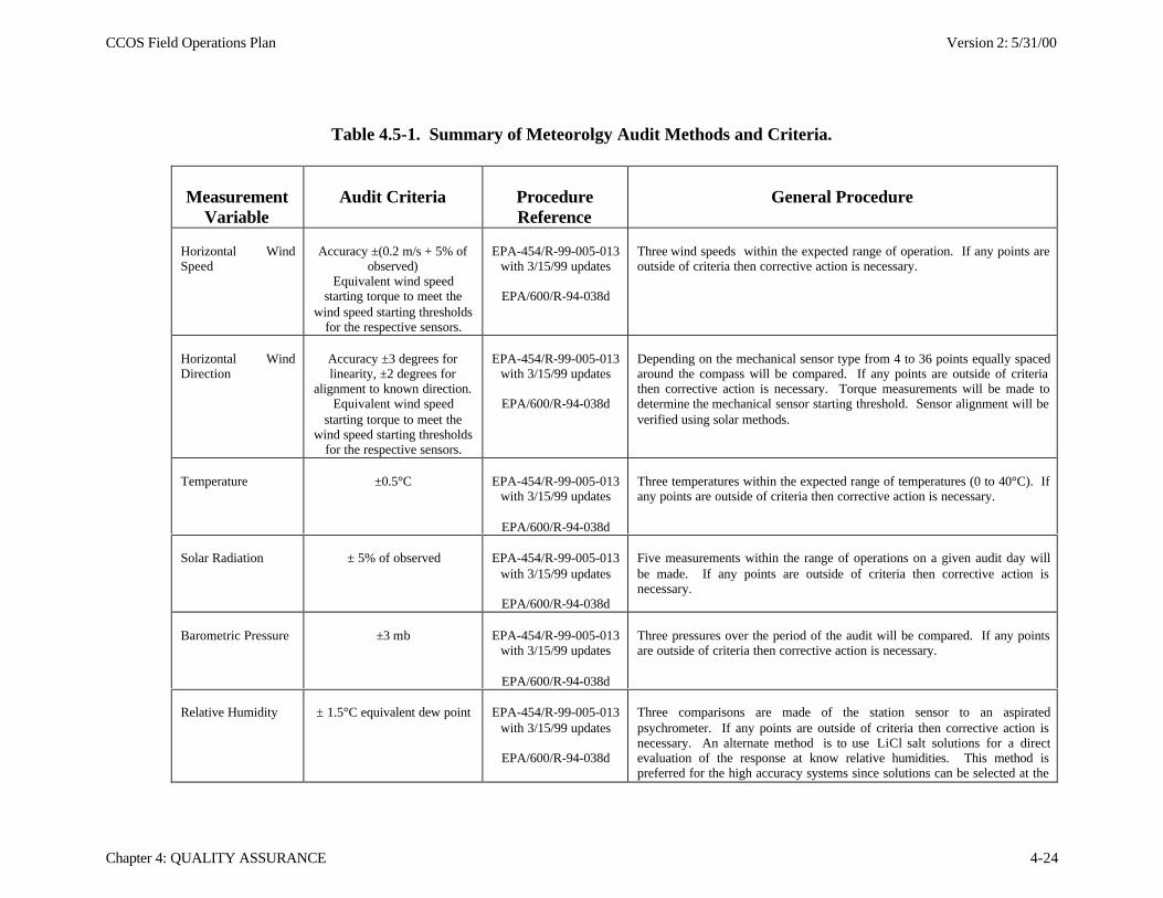
CCOS Field Operations Plan Version 2: 5/31/00
Chapter 4: QUALITY ASSURANCE 4-24
Table 4.5-1. Summary of Meteorolgy Audit Methods and Criteria.
MeasurementVariable
Audit Criteria ProcedureReference
General Procedure
Horizontal WindSpeed
Accuracy ±(0.2 m/s + 5% ofobserved)
Equivalent wind speedstarting torque to meet the
wind speed starting thresholdsfor the respective sensors.
EPA-454/R-99-005-013with 3/15/99 updates
EPA/600/R-94-038d
Three wind speeds within the expected range of operation. If any points areoutside of criteria then corrective action is necessary.
Horizontal WindDirection
Accuracy ±3 degrees forlinearity, ±2 degrees for
alignment to known direction.Equivalent wind speed
starting torque to meet thewind speed starting thresholds
for the respective sensors.
EPA-454/R-99-005-013with 3/15/99 updates
EPA/600/R-94-038d
Depending on the mechanical sensor type from 4 to 36 points equally spacedaround the compass will be compared. If any points are outside of criteriathen corrective action is necessary. Torque measurements will be made todetermine the mechanical sensor starting threshold. Sensor alignment will beverified using solar methods.
Temperature ±0.5°C EPA-454/R-99-005-013with 3/15/99 updates
EPA/600/R-94-038d
Three temperatures within the expected range of temperatures (0 to 40°C). Ifany points are outside of criteria then corrective action is necessary.
Solar Radiation ± 5% of observed EPA-454/R-99-005-013with 3/15/99 updates
EPA/600/R-94-038d
Five measurements within the range of operations on a given audit day willbe made. If any points are outside of criteria then corrective action isnecessary.
Barometric Pressure ±3 mb EPA-454/R-99-005-013with 3/15/99 updates
EPA/600/R-94-038d
Three pressures over the period of the audit will be compared. If any pointsare outside of criteria then corrective action is necessary.
Relative Humidity ± 1.5°C equivalent dew point EPA-454/R-99-005-013with 3/15/99 updates
EPA/600/R-94-038d
Three comparisons are made of the station sensor to an aspiratedpsychrometer. If any points are outside of criteria then corrective action isnecessary. An alternate method is to use LiCl salt solutions for a directevaluation of the response at know relative humidities. This method ispreferred for the high accuracy systems since solutions can be selected at the
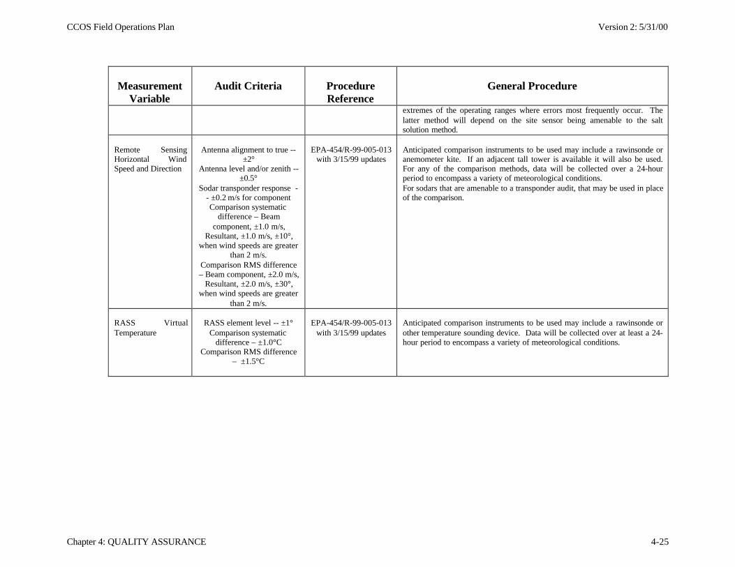
CCOS Field Operations Plan Version 2: 5/31/00
Chapter 4: QUALITY ASSURANCE 4-25
MeasurementVariable
Audit Criteria ProcedureReference
General Procedure
extremes of the operating ranges where errors most frequently occur. Thelatter method will depend on the site sensor being amenable to the saltsolution method.
Remote SensingHorizontal WindSpeed and Direction
Antenna alignment to true --±2°
Antenna level and/or zenith --±0.5°
Sodar transponder response -- ±0.2 m/s for componentComparison systematic
difference – Beamcomponent, ±1.0 m/s,
Resultant, ±1.0 m/s, ±10°,when wind speeds are greater
than 2 m/s.Comparison RMS difference– Beam component, ±2.0 m/s,
Resultant, ±2.0 m/s, ±30°,when wind speeds are greater
than 2 m/s.
EPA-454/R-99-005-013with 3/15/99 updates
Anticipated comparison instruments to be used may include a rawinsonde oranemometer kite. If an adjacent tall tower is available it will also be used.For any of the comparison methods, data will be collected over a 24-hourperiod to encompass a variety of meteorological conditions.For sodars that are amenable to a transponder audit, that may be used in placeof the comparison.
RASS VirtualTemperature
RASS element level -- ±1°Comparison systematic
difference – ±1.0°CComparison RMS difference
– ±1.5°C
EPA-454/R-99-005-013with 3/15/99 updates
Anticipated comparison instruments to be used may include a rawinsonde orother temperature sounding device. Data will be collected over at least a 24-hour period to encompass a variety of meteorological conditions.
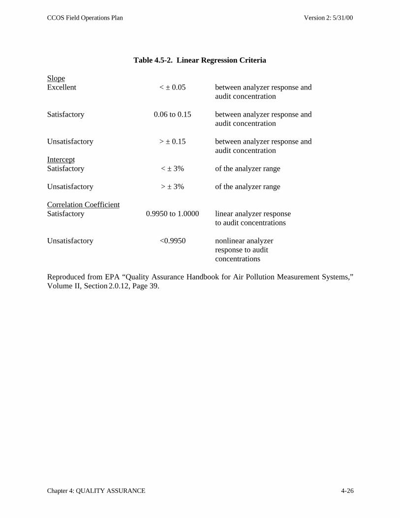
CCOS Field Operations Plan Version 2: 5/31/00
Chapter 4: QUALITY ASSURANCE 4-26
Table 4.5-2. Linear Regression Criteria
SlopeExcellent < ± 0.05 between analyzer response and
audit concentration
Satisfactory 0.06 to 0.15 between analyzer response andaudit concentration
Unsatisfactory > ± 0.15 between analyzer response andaudit concentration
InterceptSatisfactory < ± 3% of the analyzer range
Unsatisfactory > ± 3% of the analyzer range
Correlation CoefficientSatisfactory 0.9950 to 1.0000 linear analyzer response to audit concentrations
Unsatisfactory <0.9950 nonlinear analyzerresponse to auditconcentrations
Reproduced from EPA “Quality Assurance Handbook for Air Pollution Measurement Systems,”Volume II, Section 2.0.12, Page 39.
CCOS Field Operations Plan Version 2: 5/31/00
Chapter 5: DATA MANAGEMENT 5-1
5.0 DATA MANAGEMENT AND VALIDATION
The CCOS database will be compiled, documented, evaluated, and distributed by thePlanning and Technical Support Division (PTSD) of the Air Resources Board (ARB). Commondata management and validation conventions need to be assembled in a consistent and efficientmanner. These conventions are described in this section. Greg O’Brien of the ARB will serve asthe CCOS data manager. He will be responsible for establishing and maintaining computer-based data archives and managing the overall data storage and Level 1A-1B validation activities.The data manager will interact with the field manager and the program management and providefeedback to them concerning the status of unresolved data management problems and potentialfor resolution. Liz Niccum of T&B Systems will assist the CCOS data manager with datacompilation and formatting. Eric Fujita of the Desert Research Institute will assist with Level 2data validation. This draft version will be updated with more specific conventions and reportingstructures after CCOS measurement investigators have provided their suggestions andrecommendations. To the greatest extent possible, CCOS field data structures, processing,validation, and delivery procedures will be consistent with those being established for theCRPAQS (Watson et al., 1998).
5.1 Data Specifications
Data management conventions and methods for CCOS and CRPAQS build on experiencefrom and development supported by the 1990 San Joaquin Valley Air Quality Study (SJVAQS)(Blumenthal et al., 1993), the 1995 Integrated Monitoring Study (IMS-95) (Solomon andMagliano, 1997), and the 1997 Southern California Oxidant Study (SCOS-97) (Fujita et al.,1997). The following specifications are maintained by the data manager and are to be madeavailable to all project participants via the Internet:
• Monitoring Sites: Each site location for CCOS measurements is identified with aunique alphanumeric site ID accompanied by its name, address, coordinates,elevation, primary operator, and a summary of measurements taken at the site. Thefield manager with a Global Positioning System (GPS), pressure-based altimeter, andtopographical maps verify the coordinates and elevations of each site. Immediatesurroundings are recorded with a digital camera of the area surrounding the site to bedisplayed on the CCAQS web site.
• Instruments: The make, model and serial number of instruments used to acquiremeasurements at each site is recorded with its threshold, range, expected accuracyand precision.
• Parameters: Each observed parameter is assigned a unique code that is accompaniedby its definition, units, averaging time, applicable temperature and pressureadjustments, and data reporting format.
• Data validation flags: Flags specific to each measurement investigator are translatedinto a common set of validation flags that are carried with each data point. These arelisted in Section 5.3
CCOS Field Operations Plan Version 2: 5/31/00
Chapter 5: DATA MANAGEMENT 5-2
• Air Observation Data files: Basic air observation data files are constructed innormalized formats that have the same structure for different types of data.
• Time conventions: Times are expressed in Pacific Standard Time (PST), hour orminute beginning. All dates as MM/DD/YYYY (note that years are four-digit codes:.1999, 2000, 2001).
• Missing data conventions: A –99 or a “NULL” value replaces missingmeasurements. Invalidated data retain original data value and is flagged as invalid.
• Investigator code: Each measurement investigator or network operator is assigned aunique four-character code that is used to identify the source of the data. Datatransmittals will carry this code as part of the filename when they are loaded into araw data sub-directory, and a separate sub-directory on the CCOS Internet server.
5.1.1 Parameter Codes
Will be distributed by the CCOS data manager in June 2000 to CCOS participant.Includes table of VOC species
5.1.2 Investigator Codes
Will be distributed by the CCOS data manager in June 2000 to CCOS participant.
5.1.3 Measurement Codes
Will be distributed by the CCOS data manager in June 2000 to CCOS participant.
5.1.4 Methods Codes
Will be distributed by the CCOS data manager in June 2000 to CCOS participant.
5.2 Data Validation Levels
Mueller (1980), Mueller et al., (1983), and Watson et al. (1983, 1989, 1995) define athree-level data validation process that should be mandatory in any environmental measurementstudy. Data records are designated as having passed these levels by entries in the a column ofeach data file. These levels, and the validation codes that designate them, are defined as follows:
• Level 0 (ZERO): These data are obtained directly from the data loggers that acquire datain the field. Averaging times represent the minimum intervals recorded by the datalogger, which do not necessarily correspond to the averaging periods specified for thedatabase files. Level 0 data have not been edited for instrument downtime, nor haveprocedural adjustments for baseline and span changes been applied. Level 0 data are notcontained in the CCAQS database, although they are consulted on a regular basis toascertain instrument functionality and to identify potential episodes prior to receipt ofLevel 1 A data.
CCOS Field Operations Plan Version 2: 5/31/00
Chapter 5: DATA MANAGEMENT 5-3
• Level 1A (1A): These data have passed several validation tests applied by themeasurement investigator prior to data submission. The general features of Level 1A are:1) data values flagged when monitoring instruments did not function within proceduraltolerances; 2) flagging measurements when significant deviations from measurementassumptions have occurred; 3) verifying computer file entries against data sheets; 4)replacement of data from a backup data acquisition system in the event of failure of theprimary system; 5) adjustment of measurement values for quantifiable baseline and spanor interference biases; and 6) identification, investigation, and flagging of data that arebeyond reasonable bounds or that are unrepresentative of the variable being measured(e.g. high light scattering associated with adverse weather).
• Level 1B (1B): Pre-programmed consistency and reasonability tests are applied by thedata manager prior to integration into the CCAQS database. Consistency tests verify thatfile naming conventions, data formats, site codes, variable names, reporting units,validation flags, and missing value codes are consistent with project conventions.Discrepancies are reported to the measurement investigator for remediation. When thereceived files are consistent, reasonability tests are applied that include: 1) identificationof data values outside of a specified minimum or maximum value; 2) values that changeby more than a specified amount from one sample to the next; and 3) values that do notchange over a specified period. Data identified by these filters are individually examinedand verified with the data supplier. Obvious outliers (e.g. high solar radiation at midnight,300 'C temperature) are invalidated. Others may be invalidated or flagged based on theresults of the investigation. The bounds used in these tests will be determined incooperation with measurement investigators and network operators.
• Level 2 (2): Level 2 data validation takes place after data from various measurementmethods have been assembled in the master database. Level 2 validation is the first stepin data analysis. Level 2A tests involve the testing of measurement assumptions (e.g.internal nephelometer temperatures do not significantly exceed ambient temperatures),comparisons of collocated measurements (e.g. filter and continuous sulfate andabsorption), and internal consistency tests (e.g. the sum of measured aerosol species doesnot exceed measured mass concentrations). Level 2 tests also involve the testing ofmeasurement assumptions, comparisons of collocated measurements, and internalconsistency tests.
• Level 3 (3): Level 3 is applied during the model reconciliation process, when the resultsfrom different modeling and data analysis approaches are compared with each other andwith measurements. The first assumption upon finding a measurement, which isinconsistent with physical expectations, is that the unusual value is due to a measurementerror. If, upon tracing the path of the measurement, nothing unusual is found, the valuecan be assumed to be a valid result of an environmental cause. The Level 3 designation isapplied only to those variables that have undergone this reexamination after thecompletion of data analysis and modeling. Level 3 validations continue for as long as thedatabase is maintained.
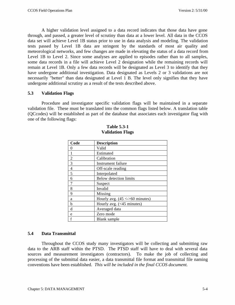
CCOS Field Operations Plan Version 2: 5/31/00
Chapter 5: DATA MANAGEMENT 5-4
A higher validation level assigned to a data record indicates that those data have gonethrough, and passed, a greater level of scrutiny than data at a lower level. All data in the CCOSdata set will achieve Level 1B status prior to use in data analysis and modeling. The validationtests passed by Level 1B data are stringent by the standards of most air quality andmeteorological networks, and few changes are made in elevating the status of a data record fromLevel 1B to Level 2. Since some analyses are applied to episodes rather than to all samples,some data records in a file will achieve Level 2 designation while the remaining records willremain at Level 1B. Only a few data records will be designated as Level 3 to identify that theyhave undergone additional investigation. Data designated as Levels 2 or 3 validations are notnecessarily "better" than data designated at Level 1 B. The level only signifies that they haveundergone additional scrutiny as a result of the tests described above.
5.3 Validation Flags
Procedure and investigator specific validation flags will be maintained in a separatevalidation file. These must be translated into the common flags listed below. A translation table(QCcodes) will be established as part of the database that associates each investigator flag withone of the following flags:
Table 5.3-1Validation Flags
Code Description0 Valid1 Estimated2 Calibration3 Instrument failure4 Off-scale reading5 Interpolated6 Below detection limits7 Suspect8 Invalid9 Missinga Hourly avg. (45 <->60 minutes)b Hourly avg. (<45 minutes)d Averaged datae Zero modef Blank sample
5.4 Data Transmittal
Throughout the CCOS study many investigators will be collecting and submitting rawdata to the ARB staff within the PTSD. The PTSD staff will have to deal with several datasources and measurement investigators (contractors). To make the job of collecting andprocessing of the submittal data easier, a data transmittal file format and transmittal file namingconventions have been established. This will be included in the final CCOS document.
CCOS Field Operations Plan Version 2: 5/31/00
Chapter 5: DATA MANAGEMENT 5-5
5.4.1 Adherence to Specifications
Data are to be provided in electronic form, validated to Level 1A by the contractor, to theCCOS Data Manager. The data format from each contractor must follow the specifications to bedefined completely in the final document, and must be approved by the CCOS Data Manager inadvance of submittal.
The contractor will submit quality control data to the data manager along with air qualityand visibility data. A precision value and a validation flag are to be reported with each measuredvalue in the database.
5.4.2 Transmittal Files
Data will be acquired at set intervals via file transfer protocol (FTP) to a pre-definedlocation set up for each measurement investigator. The files are submitted as an ASCII commadelimited text files. Comma delimited files are defined as the following:
1. Records begin at position 0.2. Records end with ASCII characters 13 (carriage return) and 10 (line feed).3. Fields are delimited with ASCII character 44 (comma).4. Character data are enclosed with ASCII character 34 (double quote).5. The end of file is indicated by ASCII character 26 (control z).
The investigator must adhere to the CCAQS Data Transmittal Convention as outlined above.
5.4.3 Transmittal File Naming Convention
The investigator must adhere to the CCAQS File Naming Convention as outlined below.Raw data file naming conventions include the investigator code, a measurement type code, andan indicator for the period of data acquisition. FTP Transmittal file names are of the formCDDMMYYA.PLL. File name conventions are listed in Table 5.3-2.
5.4.4 Transmittal Files Content
The Data Transmittal Files content convention was designed so that the quality assuranceprocess could properly identify the data source, the data of the submittal as well as qualityassuring each row of information. To ensure that each row of information, for that matter theentire transmitted file, was accurately received and recorded it must contain some of validitycheckpoints. The content convention is as follows:
1. First record, or header record, in the transmittal file identifies the record type, datasource, transmittal date, and number of air observation records in the file.
2. The next X number of records are the air observation details, where X represents thenumber of air observation records defined in header record.
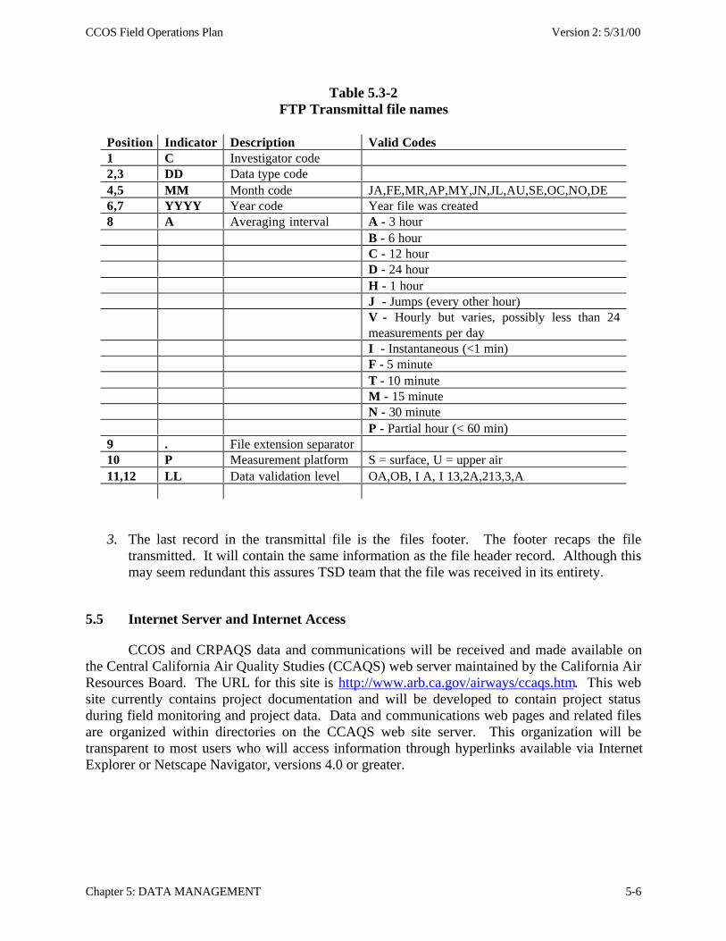
CCOS Field Operations Plan Version 2: 5/31/00
Chapter 5: DATA MANAGEMENT 5-6
Table 5.3-2FTP Transmittal file names
Position Indicator Description Valid Codes1 C Investigator code2,3 DD Data type code4,5 MM Month code JA,FE,MR,AP,MY,JN,JL,AU,SE,OC,NO,DE6,7 YYYY Year code Year file was created8 A Averaging interval A - 3 hour
B - 6 hourC - 12 hourD - 24 hourH - 1 hourJ - Jumps (every other hour)V - Hourly but varies, possibly less than 24measurements per dayI - Instantaneous (<1 min)F - 5 minuteT - 10 minuteM - 15 minuteN - 30 minuteP - Partial hour (< 60 min)
9 . File extension separator10 P Measurement platform S = surface, U = upper air11,12 LL Data validation level OA,OB, I A, I 13,2A,213,3,A
3. The last record in the transmittal file is the files footer. The footer recaps the filetransmitted. It will contain the same information as the file header record. Although thismay seem redundant this assures TSD team that the file was received in its entirety.
5.5 Internet Server and Internet Access
CCOS and CRPAQS data and communications will be received and made available onthe Central California Air Quality Studies (CCAQS) web server maintained by the California AirResources Board. The URL for this site is http://www.arb.ca.gov/airways/ccaqs.htm. This website currently contains project documentation and will be developed to contain project statusduring field monitoring and project data. Data and communications web pages and related filesare organized within directories on the CCAQS web site server. This organization will betransparent to most users who will access information through hyperlinks available via InternetExplorer or Netscape Navigator, versions 4.0 or greater.
CCOS Field Operations Plan Version 2: 5/31/00
Chapter 6: EMISSION INVENTORY DEVELOPMENT 6-1
6.0 EMISSION INVENTORY DEVELOPMENT AND EVALUATION
For a study covering as large of an area as CCOS, the development of the emissioninventory will be a major effort. In addition to the size of the study domain, the emissioninventory required for modeling is more detailed than the routine summer seasonal emissioninventory. The emission inventory (EI) needed to support the CCOS modeling will be a series ofday-specific, hourly, gridded emission inventories that cover each day of the ozone episodescaptured during the field study. To help coordinate the EI development effort, the EmissionInventory Coordination Group (EICG) has been established to determine the process forpreparing the emission inventories needed to support air quality modeling for CCOS. The EICGis chaired by Linda Murchison and Dale Shimp of the ARB. Participants in the group includemany local air districts, several local councils of government, Caltrans, California EnergyCommission, and the ARB. Local air districts participating to date include San Joaquin ValleyUnified APCD, Bay Area AQMD, Sacramento Metropolitan AQMD, Mendocino CountyAQMD, Northern Sierra AQMD, Yolo-Solano AQMD, Placer County APCD, San Luis ObispoCounty APCD, and Monterey Bay Unified APCD. Other local air districts will also beparticipating.
There are about 30 districts in the CCOS modeling domain. Each local air district in thestate updates a portion of the emission inventory for their area. An emission inventory is neededto estimate emissions for each day that will be modeled in the summer of 2000. Special effort isbeing made to assist smaller districts that have limited staffing resources. The followingsubsections the approach and schedule for developing and compiling the modeling emissioninventory, and the specific studies that have been funded in order to support this effort forCCOS.
6.1 “Fast Track” and Final Modeling Inventory Development Process
A gridded emission inventory is a critical input to photochemical air quality models.Historically, modeling emission inventories have been criticized for using incomplete day-specific data and for lagging behind the development of other data such as meteorological and airquality data that are collected in air quality studies. This subsection describes a two-trackapproach.
To make a modeling inventory available in a shorter time frame, the EICG is taking atwo-tier approach to the development of the modeling emission inventory that will providemodelers with a “fast track” inventory for preliminary modeling. This inventory will befollowed by a more detailed modeling inventory that will incorporate all of the day-specificinformation collected during the field study.
The districts and ARB will prepare a seasonal emissions inventory for 1999 duringcalendar year 2000. The 1999 annual emissions for point sources will be forecasted to 2000 andthen spatially and temporally distributed to create a modeling inventory for a summer weekday.Area source emissions for 1999 will also be forecasted to 2000. The forecasted emissions willbe spatially distributed using the spatial surrogates used in the 1994 Ozone State ImplementationPlans and temporally distributed to represent a summer weekday. On-road mobile sources willalso be gridded based on the 1994 Plans. Modelers will use this “fast track” inventory to begin
CCOS Field Operations Plan Version 2: 5/31/00
Chapter 6: EMISSION INVENTORY DEVELOPMENT 6-2
testing the performance of the photochemical model. When the 2000 annual average inventoryis ready, it will be gridded to replace the forecasted 2000 inventory. Day-specific data willreplace the gridded annual average inventory. Results from contracts will be incorporated intothe annual average inventory and/or the day-specific inventories.
6.2 Requirements for Quality Control and Quality Assurance of Emission Inventory
The EICG is placing special emphasis on ensuring consistency in emission inventorypreparation procedures between all the districts in the modeling domain. The Air ResourcesBoard will take the lead in coordinating and ensuring quality control and quality assurancestandards for the emission inventory portion of the study. Specific guidelines will be outlined forassisting state and local agencies for implementing more uniform and systematic approaches tocollecting, compiling (formats and accuracy), and reporting emission inventory data. Also, toensure good quality control practices, the EICG will be developing a comprehensive qualitycontrol and quality assurance plan. The plan will include items such as:
• Quality control checks for collecting non-emission data, updating activity data, and usingappropriate emission factors for calculating emissions;
• Emission calculation methodology;
• Updating or revising categories to ensure that the latest methodology is used;
• Data submittal;
• Data correction;
• Documentation; and
• Quality review of the entire inventory.
6.3 Proposed Contractor Studies for Emission Inventory Development
The collection of most of the emission inventory data discussed in the previous sectionswill be provided by public agencies as in-kind contributions to the CCOS study. However, thereare some critical elements of the CCOS emission inventory that the members of the EICG do nothave sufficient resources and /or expertise to provide. In general, these needs relate to the spatialand temporal distribution of emissions from motor vehicles and other area sources. Theemission inventory elements, which will need to be supported by the CCOS study, are listedbelow.
6.3.1 Day-Specific Traffic Count Information
Day-specific traffic count information will be gathered during the field study. Thesetraffic counts are used to create factors to adjust the travel demand volumes to hourly vehiclevolumes. A scoping study is planned to review the availability of traffic data and develop a
CCOS Field Operations Plan Version 2: 5/31/00
Chapter 6: EMISSION INVENTORY DEVELOPMENT 6-3
sampling plan using statistical methods for the placement of traffic counters for CCOS. Basedon the results of the scoping study, a field sampling plan will be developed to collect and analyzehourly traffic count information for the CCOS domain. The day-specific data will beincorporated into the transportation model.
6.3.2 Gridding of Area Source Emissions
Ozone and aerosol formation models require spatially distributed estimates of precursoremissions resolved over the entire geographic grid system that defines the modeling domain. Inthis project, Sonoma Technology, Inc. will develop base year and future year gridding surrogatesfor spatially distributing area source and off-road emission source categories. The spatialallocation factors will be used to geographically distribute emissions throughout the CentralCalifornia Ozone Study (CCOS) domain at a spatial resolution of 1 x 1 km covering all ofCalifornia from Shasta to Kern County.
Spatial allocation factors for area and off-road mobile sources will be developed for theyears 2000, 2005, 2010, and 2020 using various sources of data that are representative of thespatial distribution of emissions activity. These data are referred to as surrogates and commonlyinclude: demographic and socioeconomic data and land cover/land use data. STI will reviewexisting area and off-road mobile source surrogate assignments and use new and innovativemethodologies similar to those used in the 1997 South Coast Ozone Study (SCOS97) to assignsurrogates to emissions sources.
Additionally, STI will review and recommend improvements to existing temporaldistributions (hourly, daily, seasonal) of emissions activity for all area and off-road sources. Inorder to complete this project, local data will be acquired
6.3.3 Integration of Transportation Data for CCOS Domain and Run DTIM for EntireModeling Domain
The goals of this project are: 1) create gridded, hourly on-road mobile source emissionsestimates of PM, CO, NOx, and TOG which are representative of an ozone season episode and awinter episode for the base year 2000; 2) provide a cost and schedule estimate to create morerefined PM estimates (i.e. EC, OC, SO2, SO4, NH3, Na, Ca, K, Mg, and other PM in lieu of atotal PM estimate; and 3) transfer data and estimation software to the ARB and providenecessary training so that ARB staff can generate additional on-road mobile source emissionsestimates using other data sets. The contractor is Alpine Geophysics.
6.3.4 Biogenic Emission Model Expansion
Biogenic emissions are calculated using BEIGIS, the ARB’s geographic informationsystem (GIS) model for estimating biogenic hydrocarbon emissions. Although most of the majorinput databases needed to run BEIGIS currently exist, several of these databases specific to theCentral California Ozone Study (CCOS) domain require validation. The first database requiringfield validation is the spatial distribution and identification of vegetation species in natural areas,as defined by the Gap Analysis Project (GAP). The second is a 1 kilometer resolution leaf area
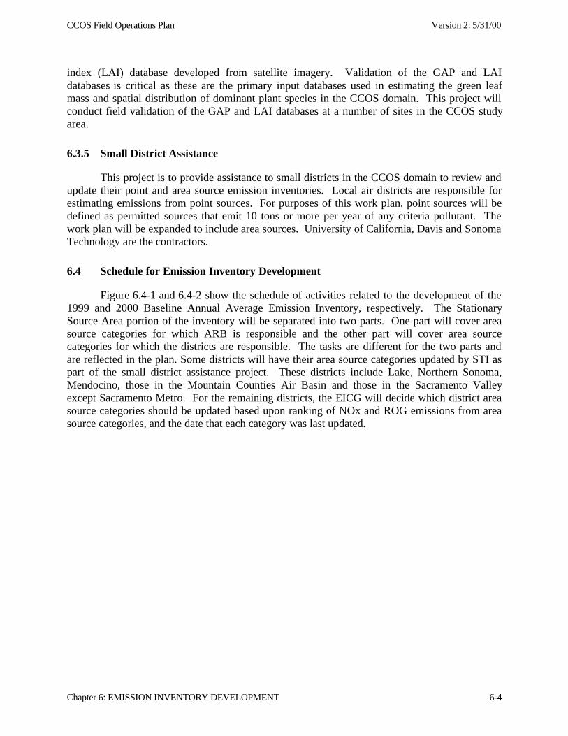
CCOS Field Operations Plan Version 2: 5/31/00
Chapter 6: EMISSION INVENTORY DEVELOPMENT 6-4
index (LAI) database developed from satellite imagery. Validation of the GAP and LAIdatabases is critical as these are the primary input databases used in estimating the green leafmass and spatial distribution of dominant plant species in the CCOS domain. This project willconduct field validation of the GAP and LAI databases at a number of sites in the CCOS studyarea.
6.3.5 Small District Assistance
This project is to provide assistance to small districts in the CCOS domain to review andupdate their point and area source emission inventories. Local air districts are responsible forestimating emissions from point sources. For purposes of this work plan, point sources will bedefined as permitted sources that emit 10 tons or more per year of any criteria pollutant. Thework plan will be expanded to include area sources. University of California, Davis and SonomaTechnology are the contractors.
6.4 Schedule for Emission Inventory Development
Figure 6.4-1 and 6.4-2 show the schedule of activities related to the development of the1999 and 2000 Baseline Annual Average Emission Inventory, respectively. The StationarySource Area portion of the inventory will be separated into two parts. One part will cover areasource categories for which ARB is responsible and the other part will cover area sourcecategories for which the districts are responsible. The tasks are different for the two parts andare reflected in the plan. Some districts will have their area source categories updated by STI aspart of the small district assistance project. These districts include Lake, Northern Sonoma,Mendocino, those in the Mountain Counties Air Basin and those in the Sacramento Valleyexcept Sacramento Metro. For the remaining districts, the EICG will decide which district areasource categories should be updated based upon ranking of NOx and ROG emissions from areasource categories, and the date that each category was last updated.
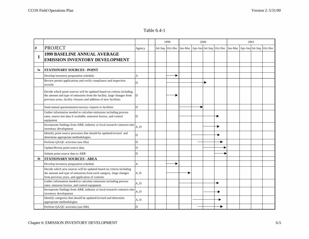
CCOS Field Operations Plan Version 2: 5/31/00
Chapter 6: EMISSION INVENTORY DEVELOPMENT 6-5
Table 6.4-1
1999 2000 2001
# PROJECT Agency Jul-Sep Oct-Dec Jan-Mar Apr-Jun Jul-Sep Oct-Dec Jan-Mar Apr-Jun Jul-Sep Oct-Dec
I1999 BASELINE ANNUAL AVERAGE EMISSION INVENTORY DEVELOPMENT
Ia STATIONARY SOURCES - POINT
Develop inventory preparation schedule A Review permit applications and verify compliance and inspection records
D
Decide which point sources will be updated based on criteria including the amount and type of emissions from the facility, large changes from previous years, facility closures and addition of new facilities
D
Send annual questionnaires/surveys /reports to facilities D Gather information needed to calculate emissions including process rates, source test data if available, emission factors, and control equipment
D
Incorporate findings from ARB, industry or local research contracts into inventory development
A, D
Identify point source processes that should be updated/revised and determine appropriate methodologies
D
Perform QA/QC activities (see IIIa) D Update/Revise point source data D Submit point source data to ARB D
Ib STATIONARY SOURCES - AREADevelop inventory preparation schedule A Decide which area sources will be updated based on criteria including the amount and type of emissions from each category, large changes from previous years, and application of controls
A, D
Gather information needed to calculate emissions including process rates, emission factors, and control equipment
A, D Incorporate findings from ARB, industry or local research contracts into inventory development
A, D
Identify categories that should be updated/revised and determine appropriate methodologies
A, D
Perform QA/QC activities (see IIIb) D
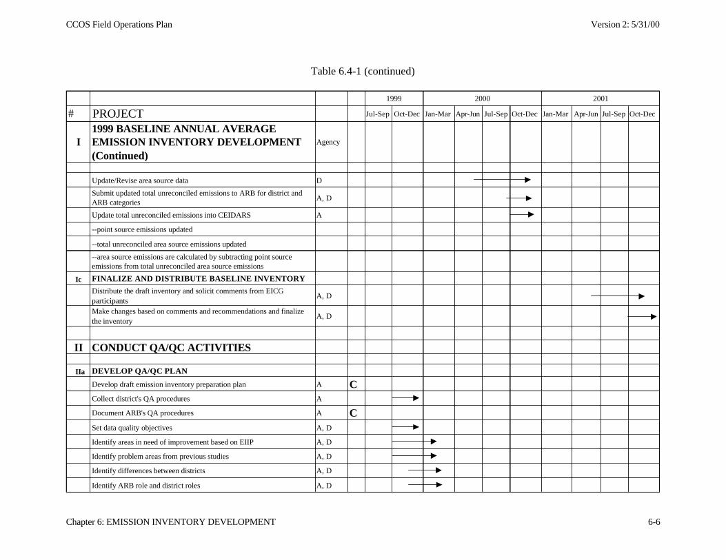
CCOS Field Operations Plan Version 2: 5/31/00
Chapter 6: EMISSION INVENTORY DEVELOPMENT 6-6
Table 6.4-1 (continued)
1999 2000 2001
# PROJECT Jul-Sep Oct-Dec Jan-Mar Apr-Jun Jul-Sep Oct-Dec Jan-Mar Apr-Jun Jul-Sep Oct-Dec
I1999 BASELINE ANNUAL AVERAGE EMISSION INVENTORY DEVELOPMENT (Continued)
Agency
Update/Revise area source data D Submit updated total unreconciled emissions to ARB for district and ARB categories
A, D
Update total unreconciled emissions into CEIDARS A
--point source emissions updated
--total unreconciled area source emissions updated
--area source emissions are calculated by subtracting point source emissions from total unreconciled area source emissions
Ic FINALIZE AND DISTRIBUTE BASELINE INVENTORY
Distribute the draft inventory and solicit comments from EICG participants
A, D
Make changes based on comments and recommendations and finalize the inventory
A, D
II CONDUCT QA/QC ACTIVITIES
IIa DEVELOP QA/QC PLAN
Develop draft emission inventory preparation plan A C Collect district's QA procedures A Document ARB's QA procedures A C Set data quality objectives A, D Identify areas in need of improvement based on EIIP A, D Identify problem areas from previous studies A, D
Identify differences between districts A, D Identify ARB role and district roles A, D
CCOS Field Operations Plan Version 2: 5/31/00
Chapter 6: EMISSION INVENTORY DEVELOPMENT 6-7
Table 6.4-1 (continued)
1999 2000 2001
# PROJECT Jul-Sep Oct-Dec Jan-Mar Apr-Jun Jul-Sep Oct-Dec Jan-Mar Apr-Jun Jul-Sep Oct-Dec
I1999 BASELINE ANNUAL AVERAGE EMISSION INVENTORY DEVELOPMENT (Continued)
Agency
Draft outline of QA plans A Develop ARB audit/review process for district data A
IIb STATIONARY SOURCES - POINT
Check the facility UTM data and assign UTM coordinates to facilities without them
D
Review facility UTM coordinates for accuracy D CJ
Review stack data and stack UTMs D Verify SCC and SIC assignments D Review temporal data for completeness and accuracy (for example, monthly throughputs)
D
Ensure all the items from the QA plan are incorporated/implemented A, D QA the device and process information provided by each facility for reasonableness
D
QA emission calculation methodology D, F Quantify variability of all emissions estimates D
Conduct visual checks, cross-check vital data, similar types of grouping A, D
Engineering audit (for facilities failing QA/QC criteria)-verify supporting documentation, i.e. source tests, MSDS; verify district's databases; verify annual emission reports
D
Identify questionable emissions and reconcile errors D
Review district data and conduct internal CEIDARS QA checks A
Conduct a reality check by comparing with previous inventory A, D
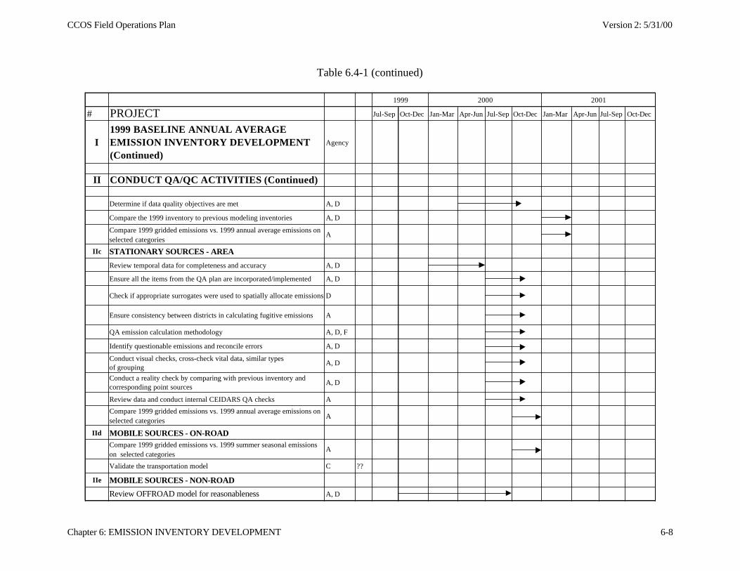
CCOS Field Operations Plan Version 2: 5/31/00
Chapter 6: EMISSION INVENTORY DEVELOPMENT 6-8
Table 6.4-1 (continued)
1999 2000 2001
# PROJECT Jul-Sep Oct-Dec Jan-Mar Apr-Jun Jul-Sep Oct-Dec Jan-Mar Apr-Jun Jul-Sep Oct-Dec
I1999 BASELINE ANNUAL AVERAGE EMISSION INVENTORY DEVELOPMENT (Continued)
Agency
II CONDUCT QA/QC ACTIVITIES (Continued)
Determine if data quality objectives are met A, D
Compare the 1999 inventory to previous modeling inventories A, D
Compare 1999 gridded emissions vs. 1999 annual average emissions on selected categories
A
IIc STATIONARY SOURCES - AREA
Review temporal data for completeness and accuracy A, D Ensure all the items from the QA plan are incorporated/implemented A, D
Check if appropriate surrogates were used to spatially allocate emissions D
Ensure consistency between districts in calculating fugitive emissions A
QA emission calculation methodology A, D, F
Identify questionable emissions and reconcile errors A, D
Conduct visual checks, cross-check vital data, similar typesof grouping
A, D
Conduct a reality check by comparing with previous inventory andcorresponding point sources
A, D
Review data and conduct internal CEIDARS QA checks A
Compare 1999 gridded emissions vs. 1999 annual average emissions on selected categories
A
IId MOBILE SOURCES - ON-ROAD
Compare 1999 gridded emissions vs. 1999 summer seasonal emissions on selected categories
A
Validate the transportation model C ??
IIe MOBILE SOURCES - NON-ROAD
Review OFFROAD model for reasonableness A, D
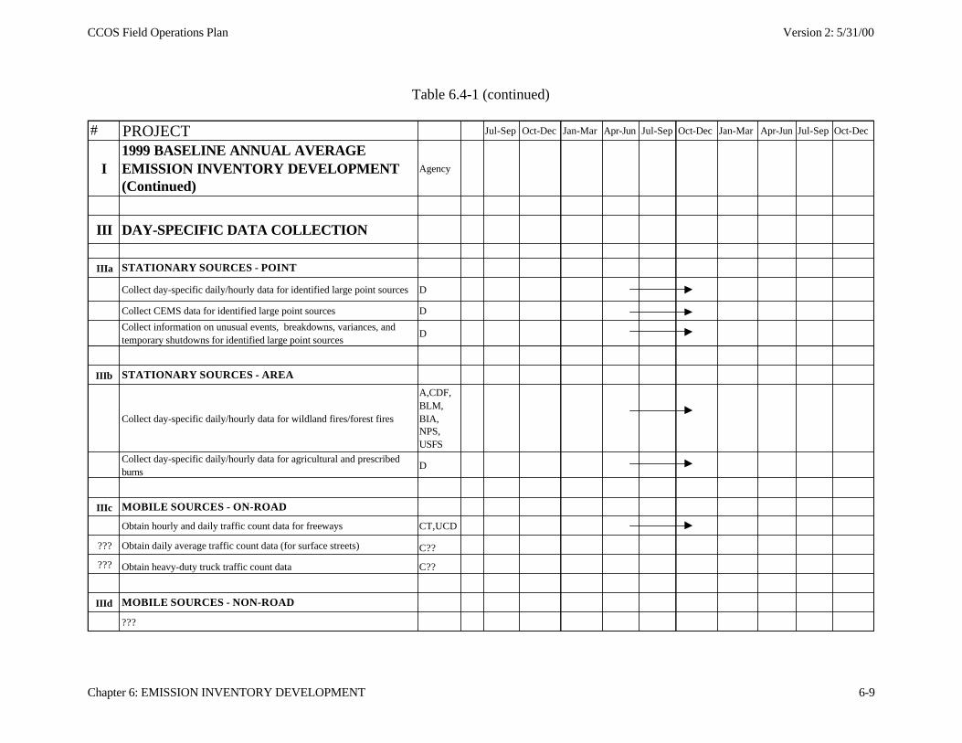
CCOS Field Operations Plan Version 2: 5/31/00
Chapter 6: EMISSION INVENTORY DEVELOPMENT 6-9
Table 6.4-1 (continued)
# PROJECT Jul-Sep Oct-Dec Jan-Mar Apr-Jun Jul-Sep Oct-Dec Jan-Mar Apr-Jun Jul-Sep Oct-Dec
I1999 BASELINE ANNUAL AVERAGE EMISSION INVENTORY DEVELOPMENT (Continued)
Agency
III DAY-SPECIFIC DATA COLLECTION
IIIa STATIONARY SOURCES - POINT
Collect day-specific daily/hourly data for identified large point sources D
Collect CEMS data for identified large point sources D
Collect information on unusual events, breakdowns, variances, and temporary shutdowns for identified large point sources
D
IIIb STATIONARY SOURCES - AREA
Collect day-specific daily/hourly data for wildland fires/forest fires
A,CDF, BLM,BIA, NPS, USFS
Collect day-specific daily/hourly data for agricultural and prescribed burns
D
IIIc MOBILE SOURCES - ON-ROAD
Obtain hourly and daily traffic count data for freeways CT,UCD
??? Obtain daily average traffic count data (for surface streets) C??
??? Obtain heavy-duty truck traffic count data C??
IIId MOBILE SOURCES - NON-ROAD
???
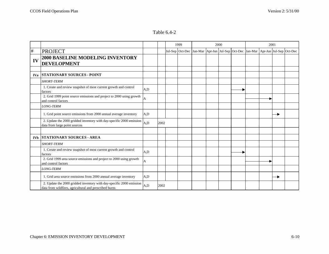
CCOS Field Operations Plan Version 2: 5/31/00
Chapter 6: EMISSION INVENTORY DEVELOPMENT 6-10
Table 6.4-2
1999 2000 2001
# PROJECT Jul-Sep Oct-Dec Jan-Mar Apr-Jun Jul-Sep Oct-Dec Jan-Mar Apr-Jun Jul-Sep Oct-Dec
IV2000 BASELINE MODELING INVENTORY DEVELOPMENT
IVa STATIONARY SOURCES - POINT
SHORT-TERM
1. Create and review snapshot of most current growth and control factors
A,D
2. Grid 1999 point source emissions and project to 2000 using growth and control factors
A
LONG-TERM
1. Grid point source emissions from 2000 annual average inventory A,D 2. Update the 2000 gridded inventory with day-specific 2000 emission data from large point sources
A,D 2002
IVb STATIONARY SOURCES - AREA
SHORT-TERM
1. Create and review snapshot of most current growth and control factors
A,D
2. Grid 1999 area source emissions and project to 2000 using growth and control factors
A
LONG-TERM
1. Grid area source emissions from 2000 annual average inventory A,D 2. Update the 2000 gridded inventory with day-specific 2000 emission data from wildfires, agricultural and prescribed burns
A,D 2002
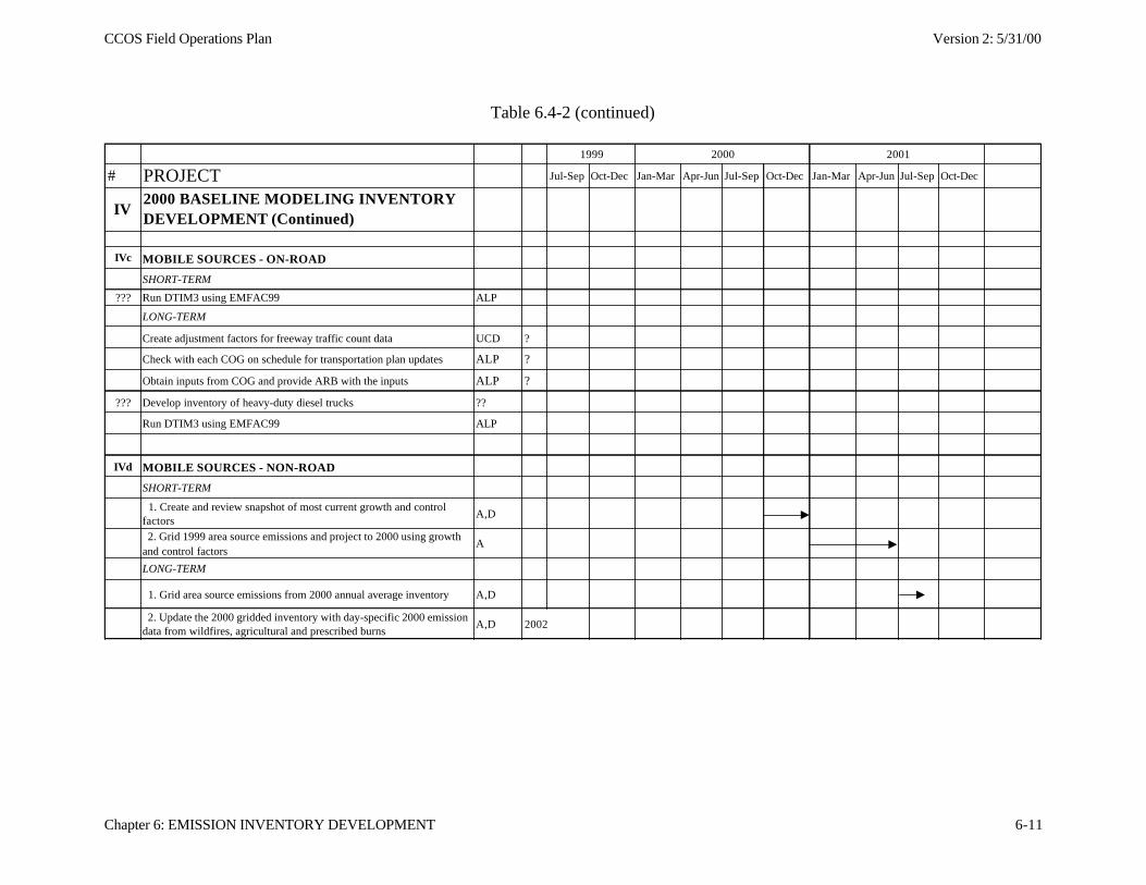
CCOS Field Operations Plan Version 2: 5/31/00
Chapter 6: EMISSION INVENTORY DEVELOPMENT 6-11
Table 6.4-2 (continued)
1999 2000 2001
# PROJECT Jul-Sep Oct-Dec Jan-Mar Apr-Jun Jul-Sep Oct-Dec Jan-Mar Apr-Jun Jul-Sep Oct-Dec
IV2000 BASELINE MODELING INVENTORY DEVELOPMENT (Continued)
IVc MOBILE SOURCES - ON-ROAD
SHORT-TERM
??? Run DTIM3 using EMFAC99 ALP
LONG-TERM
Create adjustment factors for freeway traffic count data UCD ?
Check with each COG on schedule for transportation plan updates ALP ?
Obtain inputs from COG and provide ARB with the inputs ALP ?
??? Develop inventory of heavy-duty diesel trucks ??
Run DTIM3 using EMFAC99 ALP
IVd MOBILE SOURCES - NON-ROAD
SHORT-TERM
1. Create and review snapshot of most current growth and control factors
A,D
2. Grid 1999 area source emissions and project to 2000 using growth and control factors
A
LONG-TERM
1. Grid area source emissions from 2000 annual average inventory A,D 2. Update the 2000 gridded inventory with day-specific 2000 emission data from wildfires, agricultural and prescribed burns
A,D 2002
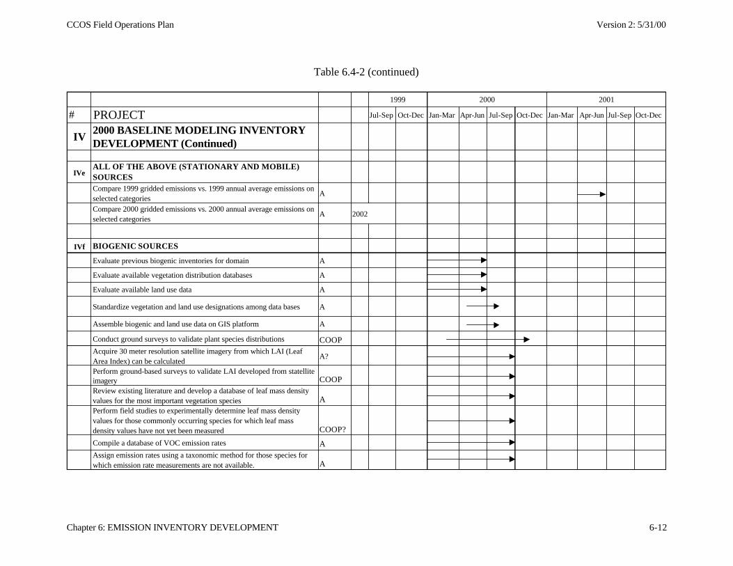
CCOS Field Operations Plan Version 2: 5/31/00
Chapter 6: EMISSION INVENTORY DEVELOPMENT 6-12
Table 6.4-2 (continued)
1999 2000 2001
# PROJECT Jul-Sep Oct-Dec Jan-Mar Apr-Jun Jul-Sep Oct-Dec Jan-Mar Apr-Jun Jul-Sep Oct-Dec
IV2000 BASELINE MODELING INVENTORY DEVELOPMENT (Continued)
IVeALL OF THE ABOVE (STATIONARY AND MOBILE) SOURCESCompare 1999 gridded emissions vs. 1999 annual average emissions on selected categories
A
Compare 2000 gridded emissions vs. 2000 annual average emissions on selected categories
A 2002
IVf BIOGENIC SOURCES
Evaluate previous biogenic inventories for domain A
Evaluate available vegetation distribution databases A
Evaluate available land use data A
Standardize vegetation and land use designations among data bases A
Assemble biogenic and land use data on GIS platform A
Conduct ground surveys to validate plant species distributions COOPAcquire 30 meter resolution satellite imagery from which LAI (Leaf Area Index) can be calculated
A?
Perform ground-based surveys to validate LAI developed from statellite imagery COOPReview existing literature and develop a database of leaf mass density values for the most important vegetation species APerform field studies to experimentally determine leaf mass density values for those commonly occurring species for which leaf mass density values have not yet been measured COOP?
Compile a database of VOC emission rates AAssign emission rates using a taxonomic method for those species for which emission rate measurements are not available. A
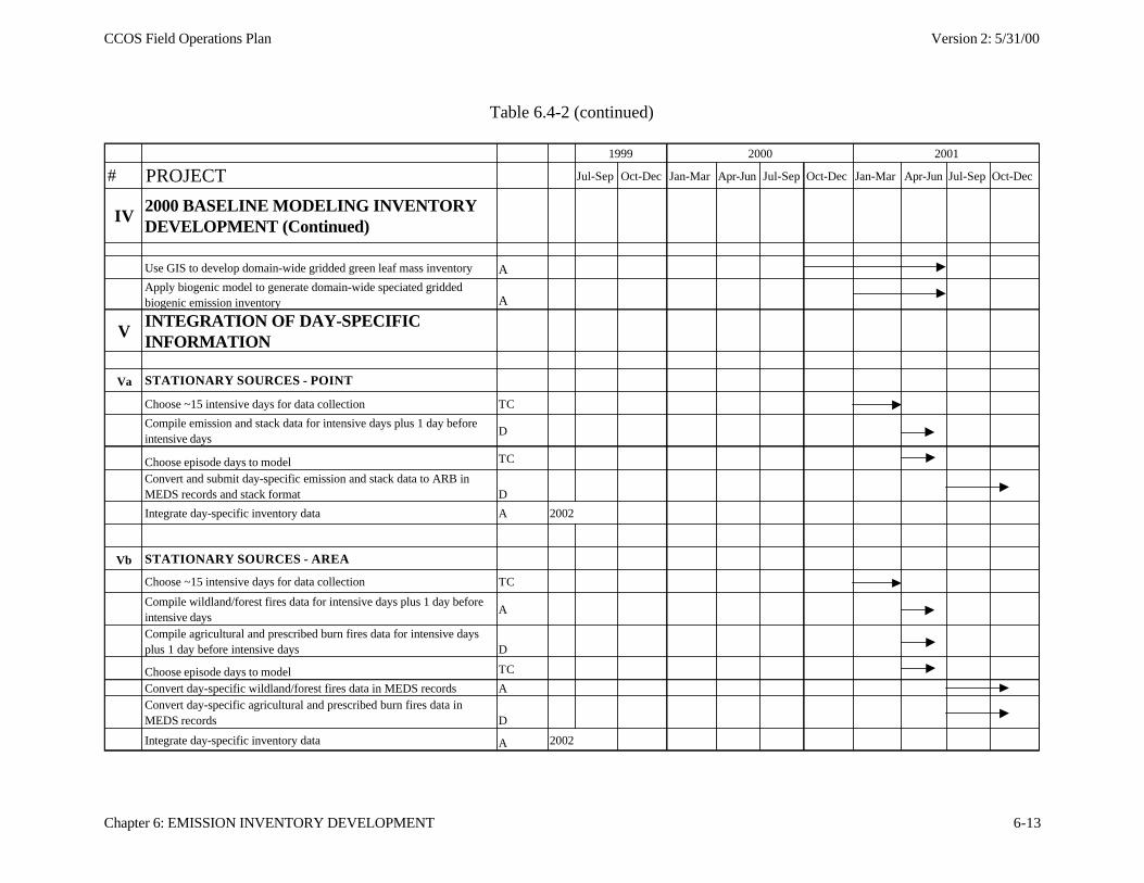
CCOS Field Operations Plan Version 2: 5/31/00
Chapter 6: EMISSION INVENTORY DEVELOPMENT 6-13
Table 6.4-2 (continued)
1999 2000 2001
# PROJECT Jul-Sep Oct-Dec Jan-Mar Apr-Jun Jul-Sep Oct-Dec Jan-Mar Apr-Jun Jul-Sep Oct-Dec
IV2000 BASELINE MODELING INVENTORY DEVELOPMENT (Continued)
Use GIS to develop domain-wide gridded green leaf mass inventory AApply biogenic model to generate domain-wide speciated gridded biogenic emission inventory A
VINTEGRATION OF DAY-SPECIFIC INFORMATION
Va STATIONARY SOURCES - POINT
Choose ~15 intensive days for data collection TC
Compile emission and stack data for intensive days plus 1 day before intensive days
D
Choose episode days to model TC
Convert and submit day-specific emission and stack data to ARB in MEDS records and stack format D
Integrate day-specific inventory data A 2002
Vb STATIONARY SOURCES - AREA
Choose ~15 intensive days for data collection TC
Compile wildland/forest fires data for intensive days plus 1 day before intensive days
A
Compile agricultural and prescribed burn fires data for intensive days plus 1 day before intensive days D
Choose episode days to model TC
Convert day-specific wildland/forest fires data in MEDS records AConvert day-specific agricultural and prescribed burn fires data in MEDS records D
Integrate day-specific inventory data A 2002
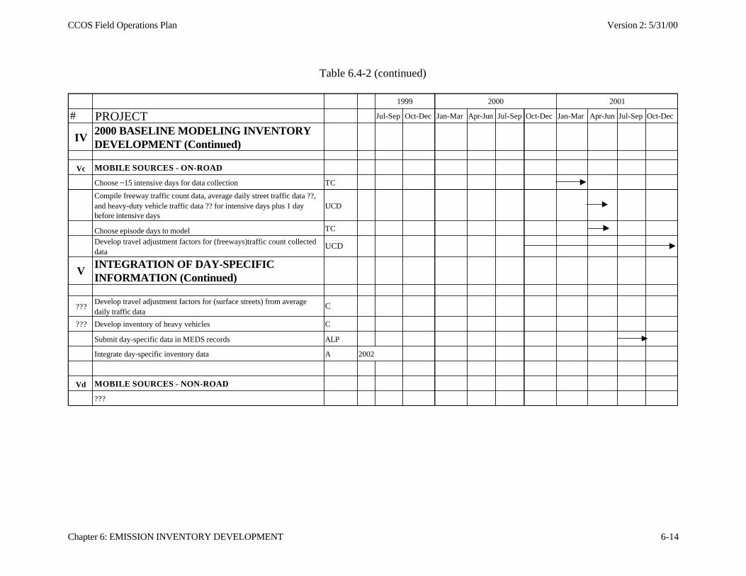
CCOS Field Operations Plan Version 2: 5/31/00
Chapter 6: EMISSION INVENTORY DEVELOPMENT 6-14
Table 6.4-2 (continued)
1999 2000 2001
# PROJECT Jul-Sep Oct-Dec Jan-Mar Apr-Jun Jul-Sep Oct-Dec Jan-Mar Apr-Jun Jul-Sep Oct-Dec
IV2000 BASELINE MODELING INVENTORY DEVELOPMENT (Continued)
Vc MOBILE SOURCES - ON-ROAD
Choose ~15 intensive days for data collection TC
Compile freeway traffic count data, average daily street traffic data ??, and heavy-duty vehicle traffic data ?? for intensive days plus 1 day before intensive days
UCD
Choose episode days to model TC
Develop travel adjustment factors for (freeways)traffic count collected data
UCD
VINTEGRATION OF DAY-SPECIFIC INFORMATION (Continued)
???Develop travel adjustment factors for (surface streets) from average daily traffic data
C
??? Develop inventory of heavy vehicles C
Submit day-specific data in MEDS records ALP
Integrate day-specific inventory data A 2002
Vd MOBILE SOURCES - NON-ROAD
???
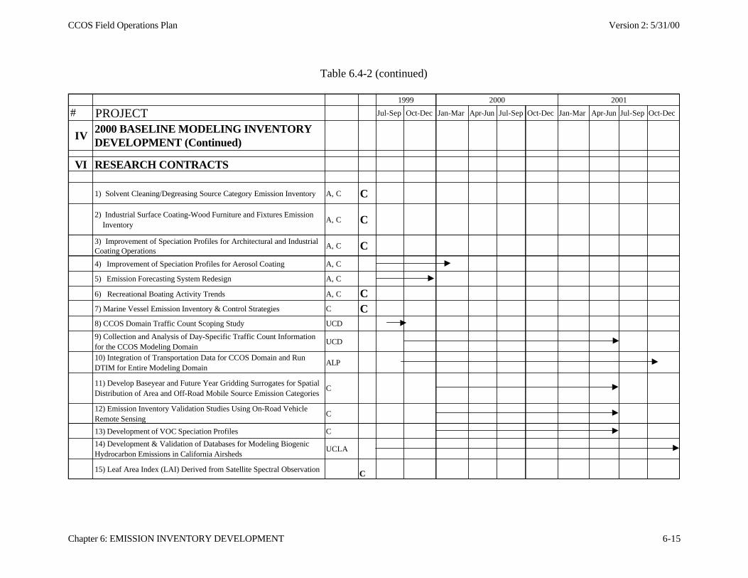
CCOS Field Operations Plan Version 2: 5/31/00
Chapter 6: EMISSION INVENTORY DEVELOPMENT 6-15
Table 6.4-2 (continued)
1999 2000 2001
# PROJECT Jul-Sep Oct-Dec Jan-Mar Apr-Jun Jul-Sep Oct-Dec Jan-Mar Apr-Jun Jul-Sep Oct-Dec
IV2000 BASELINE MODELING INVENTORY DEVELOPMENT (Continued)
VI RESEARCH CONTRACTS
1) Solvent Cleaning/Degreasing Source Category Emission Inventory A, C C
2) Industrial Surface Coating-Wood Furniture and Fixtures Emission Inventory
A, C C
3) Improvement of Speciation Profiles for Architectural and Industrial Coating Operations
A, C C
4) Improvement of Speciation Profiles for Aerosol Coating A, C
5) Emission Forecasting System Redesign A, C
6) Recreational Boating Activity Trends A, C C 7) Marine Vessel Emission Inventory & Control Strategies C C 8) CCOS Domain Traffic Count Scoping Study UCD
9) Collection and Analysis of Day-Specific Traffic Count Information for the CCOS Modeling Domain
UCD
10) Integration of Transportation Data for CCOS Domain and Run DTIM for Entire Modeling Domain
ALP
11) Develop Baseyear and Future Year Gridding Surrogates for Spatial Distribution of Area and Off-Road Mobile Source Emission Categories
C
12) Emission Inventory Validation Studies Using On-Road Vehicle Remote Sensing
C
13) Development of VOC Speciation Profiles C
14) Development & Validation of Databases for Modeling Biogenic Hydrocarbon Emissions in California Airsheds
UCLA
15) Leaf Area Index (LAI) Derived from Satellite Spectral Observation C
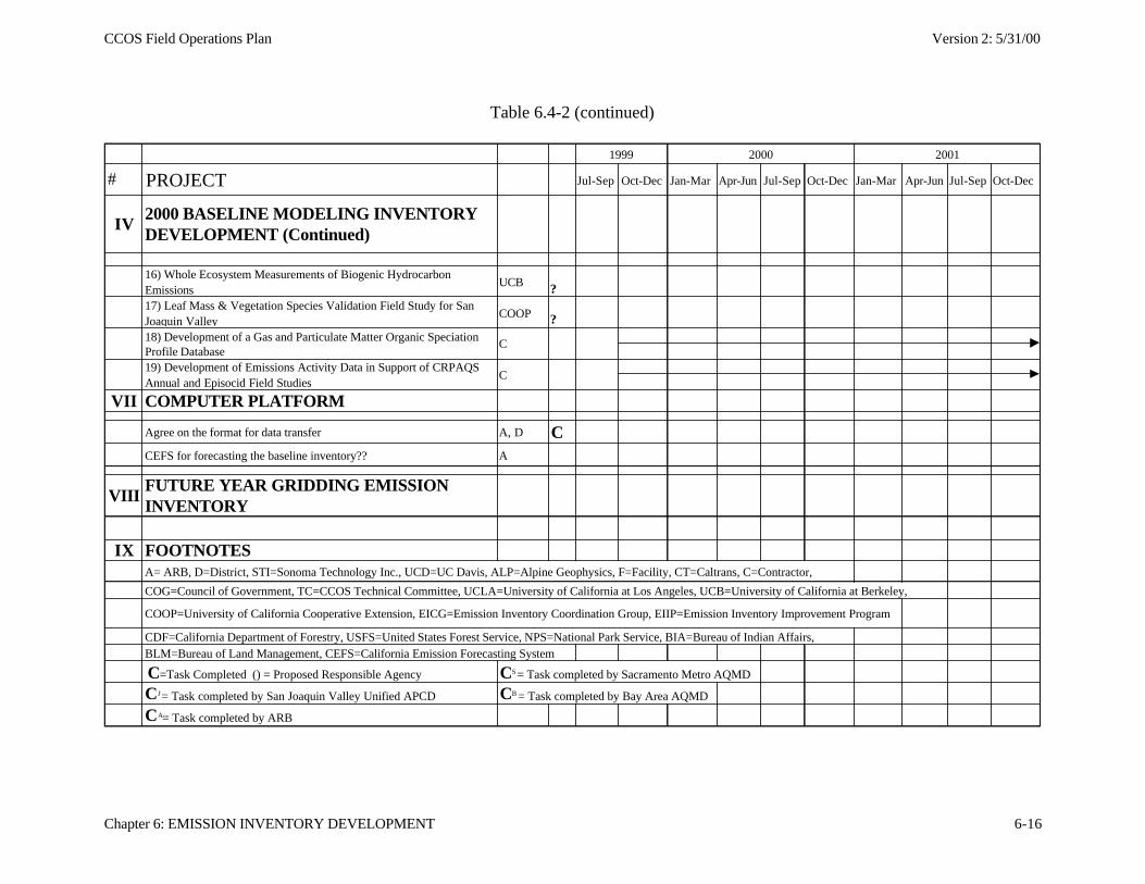
CCOS Field Operations Plan Version 2: 5/31/00
Chapter 6: EMISSION INVENTORY DEVELOPMENT 6-16
Table 6.4-2 (continued)
1999 2000 2001
# PROJECT Jul-Sep Oct-Dec Jan-Mar Apr-Jun Jul-Sep Oct-Dec Jan-Mar Apr-Jun Jul-Sep Oct-Dec
IV2000 BASELINE MODELING INVENTORY DEVELOPMENT (Continued)
16) Whole Ecosystem Measurements of Biogenic Hydrocarbon Emissions
UCB ?17) Leaf Mass & Vegetation Species Validation Field Study for San Joaquin Valley
COOP ?18) Development of a Gas and Particulate Matter Organic Speciation Profile Database
C 19) Development of Emissions Activity Data in Support of CRPAQS Annual and Episocid Field Studies
C
VII COMPUTER PLATFORM
Agree on the format for data transfer A, D C CEFS for forecasting the baseline inventory?? A
VIIIFUTURE YEAR GRIDDING EMISSION INVENTORY
IX FOOTNOTESA= ARB, D=District, STI=Sonoma Technology Inc., UCD=UC Davis, ALP=Alpine Geophysics, F=Facility, CT=Caltrans, C=Contractor,
COG=Council of Government, TC=CCOS Technical Committee, UCLA=University of California at Los Angeles, UCB=University of California at Berkeley,
COOP=University of California Cooperative Extension, EICG=Emission Inventory Coordination Group, EIIP=Emission Inventory Improvement Program
CDF=California Department of Forestry, USFS=United States Forest Service, NPS=National Park Service, BIA=Bureau of Indian Affairs, BLM=Bureau of Land Management, CEFS=California Emission Forecasting System
C=Task Completed () = Proposed Responsible Agency CS = Task completed by Sacramento Metro AQMD
CJ = Task completed by San Joaquin Valley Unified APCD CB = Task completed by Bay Area AQMD
CA= Task completed by ARB
CCOS Field Operations Plan Version 2: 5/31/00
Chapter 7: MANAGEMENT, SCHEDULE, AND BUDGET 7-1
7.0 MANAGEMENT, SCHEDULE, AND BUDGET
This section specifies the management structure and the roles of CCOS committees andworking groups, the responsibilities of field study participants, and the schedule of milestonesfor the CCOS field study and related activities. It also provides an itemized account of actualcosts and an inventory of equipment purchased with CCOS funds.
7.1 CCOS Management Structure
The CCOS is a large-scale program involving many sponsors and participants. Threeentities are involved in the overall management of the Study. The San Joaquin Valleywide AirPollution Study Agency, a joint powers agency (JPA) formed by the nine counties in the Valley,directs contracting aspects of the Study. A Policy Committee comprised of four voting blocks:State, local, and federal government, and the private sector, provides guidance on the Studyobjectives and funding levels. The Policy Committee approves all proposal requests, contractsand reports. A Technical Committee parallels the Policy Committee in membership and providesoverall technical guidance on proposal requests, direction and progress of work, contract workstatements, and reviews of all technical reports produced from the study. The leadership roles inthe CCOS field study include the principal investigators, the field coordinator, the qualityassurance officer, the data manager, the measurement investigators, the CCOS/CRPAQStechnical committee, and the CCOS/CRPAQS policy committee. On a day-to-day basis, theCalifornia Air Resources Board (ARB) is responsible for management of the Study under thedirection of the Program Manager, Chief of the Modeling and Meteorology Branch, in theARB’s Planning & Technical Support Division.
7.1.1 Policy Committee
The policy committee is composed of senior management representatives from local,state, and federal regulatory agencies and private sector stakeholders. It provides the followingpolicy and financial direction to the project.
• Provides the overall direction for the study and establishes study policy goals andobjectives.
• Evaluates CCOS technical components for their relevance to future policy decisions andassure an adequate balance among those components.
• Monitors CCOS budgets, schedules, and product quality to assure fiduciary responsibilityand fulfillment of commitments.
• Requests, justifies, and obtains sufficient sponsorship to complete defined activities thatwill achieve CCOS objectives.
• Reviews and evaluates policy-relevant CCOS findings, provides constructiverecommendations for their expression, and conveys these findings to stakeholders.
CCOS Field Operations Plan Version 2: 5/31/00
Chapter 7: MANAGEMENT, SCHEDULE, AND BUDGET 7-2
• Approve contracts to be funded by the JPA.
• Direct fund-raising efforts.
7.1.2 Technical Committee
The CCOS is directed by a technical committee that comprises staff from the CaliforniaAir Resources Board (ARB), the California Energy Commission (CEC), local air pollutioncontrol agencies, industry, and other sponsoring organizations with technical input from aconsortium of university researchers in the University of California System and the DesertResearch Institute (DRI). All contractors working on CCOS report directly to the Technicalcommittee. Members of the planning subcommittee are listed on the title page of this conceptualprogram plan. This committee provides the following technical direction to the project.
• Reviews each of the plans and recommends the final technical scope of each of theseprogram elements.
• Prepares and disseminates requests for proposals for necessary work elements andevaluates the proposals received.
• Commissions and evaluates CCOS technical reports and publications.
• Creates and monitors overall project schedules and budgets, evaluates compromisesbetween project needs and budget allocations, and institutes remedial actions whereneeded.
• Institutes, facilitates, and coordinates CCOS research activities with complementaryactivities sponsored by the local air quality management districts (i.e. BAAQMD),California Air Resources Board, U.S. Environmental Protection Agency (Region IX,ORD, and OAQPS), the Department of Defense (Naval Weapons Center), Department ofAgriculture, and industrial research sponsors (EPRI, CRC, WSPA, API).
• Participates in, to the extent possible, CCOS data acquisition, data analysis, and modelingactivities.
• Disseminates CCOS scientific findings in scientific forums, national guidancedocuments, and peer-reviewed publications.
7.1.3 Principal Investigators
The principal investigators (Andrew Ranzieri and Saffet Tanrikulu of the California AirResources Board and Eric Fujita of the Desert Research Institute) provide scientific and technicalguidance for the Central California Ozone Study. Responsibilities include:
• Create initial study protocols for data analysis, modeling, emissions characterization, andfield studies, and modify them in response to external evaluation and technical supportstudy results.
CCOS Field Operations Plan Version 2: 5/31/00
Chapter 7: MANAGEMENT, SCHEDULE, AND BUDGET 7-3
• Prepare work statements for project components.
• Working with the Technical Committee, critically review CCOS technical products andprovide constructive recommendations for improvement and focus on CCOS goals andobjectives.
• Keep informed of developments and findings in programs external to CCOS andincorporate that knowledge into CCOS planning and execution.
• Devise and refine conceptual models of elevated ozone in central California and assessthe extent to which mathematical models simulate the physical and chemical mechanismsembodied in these concepts.
• Disseminate CCOS scientific findings in scientific forums, national guidance documents,and peer-reviewed publications. Promote and facilitate the dissemination of specificresearch projects among other CCOS participants.
7.1.4 Field Study Management Team
The CCOS Management Team is responsible for making the go/no-go decisions duringthe CCOS primary study period (see Section 3.3). The Management Team consists of seniortechnical representatives from the ARB (Don McNerny and Andrew Ranzieri), BAAQMD (RobDeMandel), SMAQMD (Bridget Tollstrup), and SJVUAPCD (Dave Jones) with input from theForecast Team leader (Saffet Tanrikulu) and the CCOS Field Manager (Eric Fujita).
7.1.5 Meteorological Working Group and Forecast Team
A Meteorological Working Group (MWG) was established to update informationregarding the meteorological scenarios associated with ozone exceedances in various areas of themodeling domain. This team includes representatives from the ARB, BAAQMD, SMAQMD,and SJVUAPCD (see page ii). The CCOS Forecast Team was formed from the MWG (seeSection 3.2). The forecast team develops the Forecast Plan in conjunction with the field manager,reviews meteorological data, and provides consensus forecasts to the CCOS Management Team.The forecast team also documents the daily meteorological conditions during the study.
7.1.6 Field Manager
The implementation and coordination of the experimental phase of the CCOS will be theresponsibility of the field manager (Eric Fujita, Desert Research Institute).
• Select sampling sites based on the monitoring purposes and criteria stated in this plan anddocument those sites with respect to their location and surroundings.
• Maintain current information on equipment procurement and installation, qualityassurance, schedule, and budget sections of the field operations plan.
CCOS Field Operations Plan Version 2: 5/31/00
Chapter 7: MANAGEMENT, SCHEDULE, AND BUDGET 7-4
• Prepare work statements for different components of the field measurement program.
• Establish an efficient communications network, including a project roster of names,addresses, phone numbers, fax numbers, and e-mail addresses among other field studyparticipants and apply that network to convey needed information among the participants.
• Participate in the evaluation of technical proposals from measurement investigators andprovide perspective on the likelihood that different measurement alternatives willaccomplish measurement objectives.
• Identify and resolve communications difficulties among measurement investigators, thedata manager, and the quality assurance officer to assure that audit findings are correctedand documented and that data flow efficiently and smoothly into the project database.
• Develop a protocol to disseminate go/nogo and abort decisions.
• The field coordinator is responsible for seeing that the planned quality assurance programis implemented, measurement plans are followed, and corrective action is takenimmediately as problems arise.
• Document measurement activities and field program activities in a formal report. Thisreport will include site descriptions and a list of participants and measurement activities,as well as a daily log of events during intensive studies. It will incorporate the relevantinformation from the field protocol document, as well as the pertinent information fromthe field project log including but not limited to daily forecasts, and a daily log ofmeasurement activities.
7.1.7 Field Facilities Coordinator
Installation of required infrastructure at CCOS supplemental air quality andmeteorological sites is the responsibility of the Field Facilities Coordinator (Chuck McDade,ENSR). In addition to evaluating proposed study sites, the role of siting also includes obtainingall necessary permits, meeting indemnification and insurance requirements for access, ensuringcompliance with local and state environmental and safety regulations, and arranging for studyneeds at the site, including trailers, fencing, power and telephone.
7.1.8 Quality Assurance Manager
The quality assurance manager provides direction, coordination, and documentation ofmeasurement accuracy, precision, and validity. Specifically, the quality assurance officer will:
• Prepare a quality assurance program plan that specifies systems and performance auditingmethods, intercomparison methods, primary and transfer standards, schedules, auditreporting formats, feedback to measurement investigators, and methods to verify thatremedial actions have been taken.
CCOS Field Operations Plan Version 2: 5/31/00
Chapter 7: MANAGEMENT, SCHEDULE, AND BUDGET 7-5
• Assemble and direct a quality assurance team with specialized expertise and equipment inevaluating precision, accuracy, and validity of established and developing measurementmethods. Deploy this team to conduct systems and performance audits, assemble theresults, provide feedback to measurement investigators, and verify that remedial actionshave been implemented.
• Analyze data from collocated or nearby air quality and meteorological measurementsystems to estimate precision, equivalence, and predictability among measurements.Identify environmental and atmospheric composition conditions under which values forthese attributes are acceptable and unacceptable.
• Identify, obtain, and evaluate standard operating procedures for methods to be appliedduring field studies.
• Evaluate data qualification statements prepared by measurement investigators.
7.1.9 Measurement Investigators
Measurement investigators are responsible for specialized CCOS measurements.Specifically, measurement investigators will:
• Specify and procure (or construct) monitoring devices and verify their adequacy foroperation under conditions anticipated during CCOS field monitoring.
• Specify for the field manager space, power, supplies, storage, shipping/receiving,environmental, and communications requirements for each monitoring site at which theinvestigator's measurements will be acquired.
• Develop or adapt standard operating procedures and checklists and participate in trainingof site operators, or supply specially-trained site operators as needed.
• Install and calibrate instruments at the measurement sites and remove them after studycompletion.
• Supply expendables needed to maintain measurement schedules.
• Monitor network operations, in collaboration with the field coordinator, identify andremediate deficiencies.
• Evaluate and remediate system and performance audit findings and document thatremediation.
• Regularly acquire raw measurements to evaluate monitor performance. Periodicallyreduce data, validate it at Level 1A, and deliver it in the prescribed formats to the datamanager.
CCOS Field Operations Plan Version 2: 5/31/00
Chapter 7: MANAGEMENT, SCHEDULE, AND BUDGET 7-6
• Prepare a summary of monitoring methods, data and validation results, and measurementactivities when measurements have been completed. Prepare data quality statements thatevaluate the accuracy, precision, validity, and completeness of the measurementsacquired during each phase of the field study.
7.1.10 Emissions Inventory Working Group
There are about 30 districts in the CCOS modeling domain. Each local air district in thestate updates a portion of the emission inventory for their area. To help coordinate this effort,the Emission Inventory Coordination Group (EICG) has been established to determine theprocess for preparing the emission inventories needed to support air quality modeling for CCOS.Participants in the group include many local air districts, several local councils of government,Caltrans, California Energy Commission, and the ARB. Local air districts participating to dateinclude San Joaquin Valley Unified APCD, Bay Area AQMD, Sacramento MetropolitanAQMD, Mendocino County AQMD, Northern Sierra AQMD, Yolo-Solano AQMD, PlacerCounty APCD, San Luis Obispo County APCD, and Monterey Bay Unified APCD. The EICG ischaired by Linda Murchison and Dale Shimp of the Air Resources Board.
7.1.11 Data Manager
The data manager (Greg O’Brien, ARB) will establish and maintain computer-based dataarchives and communications. Specifically, the data manager will:
• Review and revise the data management section of this plan as changes are made to datareporting, structure, and retrieval conventions.
• Define and procure hardware and software needed to successfully complete the datamanagement tasks.
• Prepare statements of work and direct data management support investigators to assist inthe accomplishment of data management tasks.
• Establish a CCOS web page with links to: 1) long-term data archives; 2) electronic copiesof CCOS reports and documents (electronic form); 3) CCOS participants’ roster, roles,and websites (where available); and 4) standard operating procedures; 5) data receiptarchives; 6) CCOS field study data archives; and 7) measurement sites and observables.
• Develop, apply, and document efficient and modern methods for receiving, processing,and delivering data from and to measurement, data analysis, and modeling investigators.
• Perform Level 1B validation tests. Apply Level II and III validation adjustments andflags.
CCOS Field Operations Plan Version 2: 5/31/00
Chapter 7: MANAGEMENT, SCHEDULE, AND BUDGET 7-7
7.1.12 Data Analysis and Modeling Investigators
Data analysis and modeling investigators will use the integrated data set to perform Level2 and Level 3 data validation, to further answer the questions posed in Section 3, and to develop,evaluate, and apply source and receptor models. Several of the data analysis activities,especially those involved with determining Level 2 validation status of measurements anddescriptive analysis of the measurements, are best performed by the measurement investigators.Specifically, data analysis and modeling investigators will:
• Evaluate the consistency of measurements, i.e. Level 2 validation.
• Describe statistical, temporal, and spatial distributions of measurements on average andduring episodes.
• Interpret data to address data analysis objectives specified in Section 1.2.
• Recommend revisions to the conceptual models in Section 3 of the Field Study Plan(Fujita et al., 1999), elaborating on the dominance and validity of chemical and physicalmechanisms and the importance of different pollution sources.
• Use field measurements in meteorological and air quality source and receptor models toevaluate the extent to which they represent the identified mechanisms and emissions.
• Use field measurements to establish base cases for several different episodes ofmaximum concentration to evaluate the effects of different emissions reductionstrategies.
• Identify data deficiencies and initiate Level 3 validation checks and corrections with thedata manager.
• Select the most suitable modeling systems (for meteorology, emissions, and air quality)for representing photochemical air pollution in central and northern California.
• Specify model domain boundaries, boundary conditions, initial conditions, chemicalmechanisms, aerosol module, plume-in-grid module, grid sizes, layers, and surfacecharacteristics.
• Identify performance evaluation methods and performance measures, and specifymethods by which these will be applied.
• Evaluate the results of the meteorological model.
• Perform operational evaluation of the air quality model.
• Evaluate and improve the performance of emissions, meteorological, and air qualitysimulations. Apply simulation methods to estimate ozone concentrations at receptor sitesand to test potential emissions reduction strategies.
CCOS Field Operations Plan Version 2: 5/31/00
Chapter 7: MANAGEMENT, SCHEDULE, AND BUDGET 7-8
• Identify the limiting precursors of ozone and assess the extent to which reductions involatile organic compounds and nitrogen oxides, would be effective in reducing ozoneconcentrations.
• Characterize the structure and evolution of the boundary layer and the nature of regionalcirculation patterns that determine the transport and diffusion of ozone and its precursorsin northern and central California.
• Identify and describe transport pathways between neighboring air basins, and estimate thefluxes of ozone and precursors transported at ground level and aloft under differingmeteorological conditions. Reconcile results with flux plane measurements.
• Determine the contribution of ozone generated from emissions in one basin to federal andstate exceedances in neighboring air basin through emission reduction sensitivityanalysis.
7.2 Schedule
Table 7.2-1 provides milestones for CCOS field study and related activities. Thisschedule is integrated with the master project schedule that includes emissions and modelingactivities. The overall time scale shown is four years.
7.3 Budget
The total budget for CCOS is $8,170,000. Contract and other costs are itemized in Table7.3-1. Tables 7.3-2 and 7.3-3 itemize the cost of equipment and supplies purchased from theCCOS equipment and contingency funds, and equipment supplied through contracts andCRPAQS, respectively. In addition to the above contract costs, the ARB and the local APCD’sare committing in-kind resources for planning and execution of CCOS. Estimates of in-kindcosts are estimated by multiplying the projected level of effort (in hours) by a nominal hourlyrate. In-kind costs include additional efforts that are specifically required during CCOS and doesnot include data collection and analysis associated with normal daily operations (e.g., PAMS andother aerometric monitoring programs). The in-kind costs total $1,369,000, which does notinclude substantial leveraging of resources that will be available from CRPAQS. Participation ofthe Department of Energy Gulfstream 159 (G-1) aircraft is funded through the AtmosphericChemistry Program.
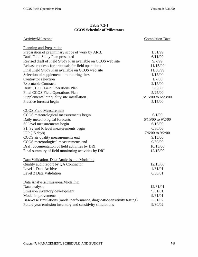
CCOS Field Operations Plan Version 2: 5/31/00
Chapter 7: MANAGEMENT, SCHEDULE, AND BUDGET 7-9
Table 7.2-1CCOS Schedule of Milestones
Activity/Milestone Completion Date
Planning and PreparationPreparation of preliminary scope of work by ARB. 1/31/99Draft Field Study Plan presented 6/11/99Revised draft of Field Study Plan available on CCOS web site 9/7/99Release requests for proposals for field operations 11/15/99Final Field Study Plan available on CCOS web site 11/30/99Selection of supplemental monitoring sites 1/15/00Contractor selection 1/7/00Executable Contracts 2/15/00Draft CCOS Field Operations Plan 5/5/00Final CCOS Field Operations Plan 5/25/00Supplemental air quality site installation 5/15/00 to 6/23/00Practice forecast begin 5/15/00
CCOS Field MeasurementCCOS meteorological measurements begin 6/1/00Daily meteorological forecasts 6/15/00 to 9/2/00S0 level measurements begin 6/15/00S1, S2 and R level measurements begin 6/30/00IOP (15 days) 7/6/00 to 9/2/00CCOS air quality measurements end 9/15/00CCOS meteorological measurements end 9/30/00Draft documentation of field activities by DRI 10/15/00Final summary of field monitoring activities by DRI 12/15/00
Data Validation, Data Analysis and ModelingQuality audit report by QA Contractor 12/15/00Level 1 Data Archive 4/31/01Level 2 Data Validation 6/30/01
Data Analysis/Emissions/ModelingData analysis 12/31/01Emission inventory development 9/31/01Model improvements 9/31/01Base-case simulations (model performance, diagnostic/sensitivity testing) 3/31/02Future year emission inventory and sensitivity simulations 9/30/02
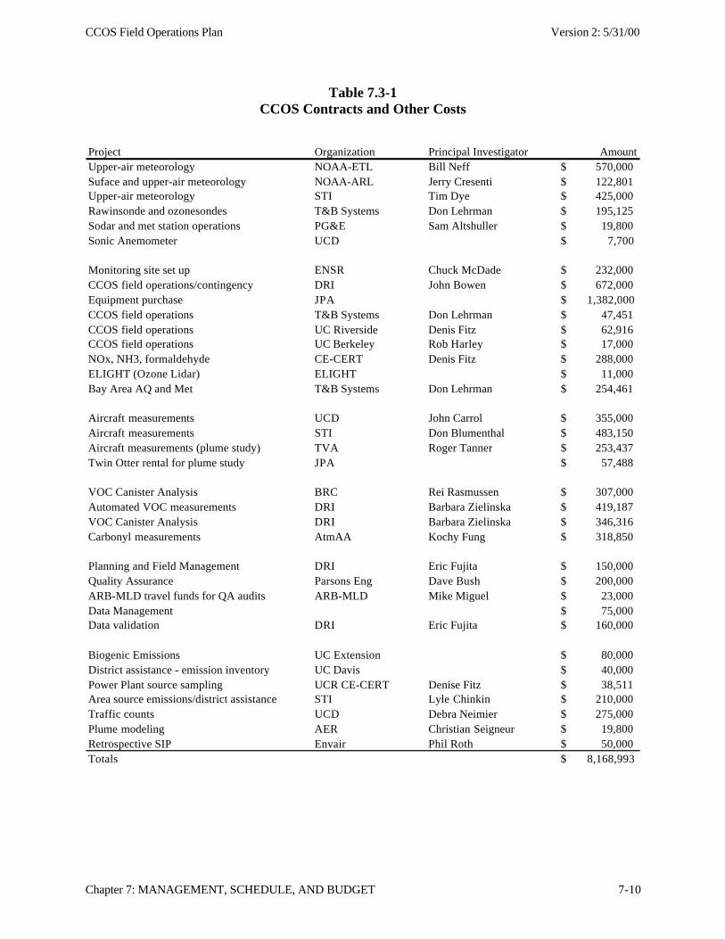
CCOS Field Operations Plan Version 2: 5/31/00
Chapter 7: MANAGEMENT, SCHEDULE, AND BUDGET 7-10
Table 7.3-1CCOS Contracts and Other Costs
Project Organization Principal Investigator AmountUpper-air meteorology NOAA-ETL Bill Neff 570,000$ Suface and upper-air meteorology NOAA-ARL Jerry Cresenti 122,801$ Upper-air meteorology STI Tim Dye 425,000$ Rawinsonde and ozonesondes T&B Systems Don Lehrman 195,125$ Sodar and met station operations PG&E Sam Altshuller 19,800$ Sonic Anemometer UCD 7,700$
Monitoring site set up ENSR Chuck McDade 232,000$ CCOS field operations/contingency DRI John Bowen 672,000$ Equipment purchase JPA 1,382,000$ CCOS field operations T&B Systems Don Lehrman 47,451$ CCOS field operations UC Riverside Denis Fitz 62,916$ CCOS field operations UC Berkeley Rob Harley 17,000$ NOx, NH3, formaldehyde CE-CERT Denis Fitz 288,000$ ELIGHT (Ozone Lidar) ELIGHT 11,000$ Bay Area AQ and Met T&B Systems Don Lehrman 254,461$
Aircraft measurements UCD John Carrol 355,000$ Aircraft measurements STI Don Blumenthal 483,150$ Aircraft measurements (plume study) TVA Roger Tanner 253,437$ Twin Otter rental for plume study JPA 57,488$
VOC Canister Analysis BRC Rei Rasmussen 307,000$ Automated VOC measurements DRI Barbara Zielinska 419,187$ VOC Canister Analysis DRI Barbara Zielinska 346,316$ Carbonyl measurements AtmAA Kochy Fung 318,850$
Planning and Field Management DRI Eric Fujita 150,000$ Quality Assurance Parsons Eng Dave Bush 200,000$ ARB-MLD travel funds for QA audits ARB-MLD Mike Miguel 23,000$ Data Management 75,000$ Data validation DRI Eric Fujita 160,000$
Biogenic Emissions UC Extension 80,000$ District assistance - emission inventory UC Davis 40,000$ Power Plant source sampling UCR CE-CERT Denise Fitz 38,511$ Area source emissions/district assistance STI Lyle Chinkin 210,000$ Traffic counts UCD Debra Neimier 275,000$ Plume modeling AER Christian Seigneur 19,800$ Retrospective SIP Envair Phil Roth 50,000$ Totals 8,168,993$
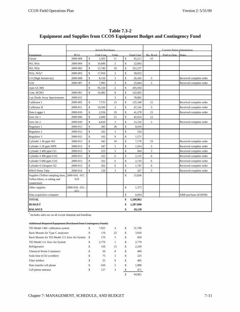
CCOS Field Operations Plan Version 2: 5/31/00
Chapter 7: MANAGEMENT, SCHEDULE, AND BUDGET 7-11
Table 7.3-2Equipment and Supplies from CCOS Equipment Budget and Contingency Fund
Actual Purchases Current Status Information
Equipment PO # Unit Cost Units Total Cost 1
No. Rcvd Paid to Date NotesOzone 2000-009 5,503$ 11 65,211$ 10
NO, NOx 2000-004 10,600$ 2 22,843$
NO, NOy 2000-002 15,740$ 19 322,237$
NOy, NOy* 2000-003 17,950$ 3 58,023$
CO (High Sensitivity) 2000-008 8,150$ 3 26,345$ 3 Received complete order
CO2 2000-007 7,995$ 3 25,844$ 3 Received complete order
Auto GC/MS 95,150$ 2 205,050$
Cont. HCHO 2000-001 16,482$ 8 142,003$
2-pi Diode Array Spectrometer 2000-015 3 78,882$
Calibrator I 2000-005 7,755$ 15 125,340$ 15 Received complete order
Calibrator II 2000-011 14,500$ 3 47,141$ 3 Received complete order
Data Logger I 2000-010 2,556$ 19 41,278$ 15 Received complete order
Zero Air 1 2000-006 2,600$ 15 42,023$ 12
Zero Air 2 2000-020 4,650$ 3 15,532$ 3 Received complete order
Regulator 1 2000-012 285$ 28 8,618$
Regulator 2 2000-012 162$ 3 524$
Regulator 3 2000-012 162$ 9 1,571$
Cylinder 1 40 ppm NO 2000-013 342$ 19 7,170$ 19 Received complete order
Cylinder 2 20 ppm NPN 2000-013 347$ 5 1,914$ 5 Received complete order
Cylinder 3 400 ppm CO 2000-013 253$ 3 844$ 3 Received complete order
Cylinder 4 300 ppm CO2 2000-013 322$ 6 2,135$ 6 Received complete order
Cylinder 5 600 ppm CO2 2000-013 322$ 6 2,135$ 6 Received complete order
Cylinder 6 Ultrapure N2 2000-013 262$ 6 1,747$ 6 Received complete order
HNO3 Perm Tube 2000-014 129$ 3 427$ 3 Received complete order
Supplies (Teflon sampling lines, Teflon filters, ss tubing and connectors)
2000-016, -017, -019
15,836$
Other supplies 2000-018, -021, -022
1,372$
Data acquisition computer 6,818$ ARB purchase (4/28/00)
TOTAL 1,268,862$
BUDGET 1,287,000$
BALANCE 18,138$ 1 Includes sales tax on all except shipping and handling.
Additional Required Equipment (Purchased from Contingency Funds)
TEI Model 146C calibration system 7,925$ 4 31,700$
Rack Mounts for Type C analyzers 170$ 23 3,910$
Rack Mounts for TEI Model 111 Zero Air System 170$ 5 850$
TEI Model 111 Zero Air System 2,770$ 1 2,770$
Refrigerators 150$ 15 2,250$
Chemical Waste Containers 50$ 8 400$
Soda lime (CO2 scrubber) 75$ 3 225$
Filter holders 55$ 9 495$
Data transfer cell phone 630$ 3 1,890$
Cell phone antenna 157$ 3 471$
44,961$
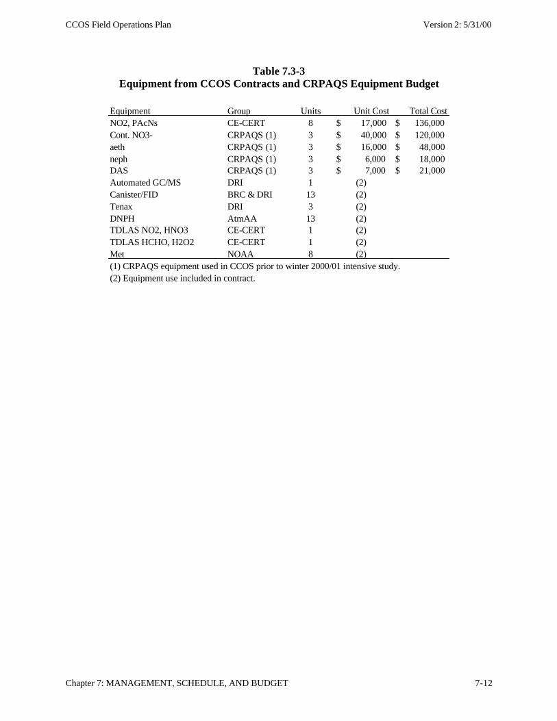
CCOS Field Operations Plan Version 2: 5/31/00
Chapter 7: MANAGEMENT, SCHEDULE, AND BUDGET 7-12
Table 7.3-3Equipment from CCOS Contracts and CRPAQS Equipment Budget
Equipment Group Units Unit Cost Total CostNO2, PAcNs CE-CERT 8 17,000$ 136,000$ Cont. NO3- CRPAQS (1) 3 40,000$ 120,000$ aeth CRPAQS (1) 3 16,000$ 48,000$ neph CRPAQS (1) 3 6,000$ 18,000$ DAS CRPAQS (1) 3 7,000$ 21,000$ Automated GC/MS DRI 1 (2)Canister/FID BRC & DRI 13 (2)Tenax DRI 3 (2)DNPH AtmAA 13 (2)TDLAS NO2, HNO3 CE-CERT 1 (2)TDLAS HCHO, H2O2 CE-CERT 1 (2)Met NOAA 8 (2)(1) CRPAQS equipment used in CCOS prior to winter 2000/01 intensive study.(2) Equipment use included in contract.
CCOS Field Operations Plan Version 2: 5/31/00
Chapter 8: REFERENCES 8-1
8.0 REFERENCES
Altshuler, S.L., T.D. Arcado, and D.R. Lawson. (1995). Weekend vs. Weekday Ambient OzoneConcentrations: Discussion and Hypotheses with Focus on Northern California. J. AirWaste Manage. Assoc., 45, 967-972.
Blier, W., A.M. Winer, D. Hansen and R. Chavira (1998). Analysis of Weekday/WeekendDifferences in Ambient Air Quality and Meteorology in the South Coast Air Basin. Draftfinal report prepared by the Department of Atmospheric Sciences and EnvironmentalScience and Engineering, University of California, Los Angeles for the California AirResources Board, Sacramento CA, under contract No. 95-334, February, 1998
Elkus, B. and K.R. Wilson (1977). Photochemical Air Pollution: Weekend-weekday differences.Atmospheric Environment, 11, 509-515.
Environmental Test Laboratory, 1994: A multi-year observational study of atmospheric transportcorridors and processes in California. Prepared for the California Air Resources Board byETL/NOAA 325 Broadway, Boulder CO 80303, May 1994.
EPA. Guideline for reporting of daily air quality – air quality index (AQI). EPA-454/R-99-010,July 1999. Research Triangle Park, NC, U.S. EPA, OAQPS.
Fairley, D. and R. DeMandel, 1996: An Analysis of SARMAP Episode Day Representativeness,Final report. Prepared for the SARMAP Data Analysis Project by the Bay Area AirQuality Management District, San Francisco, CA, Faust, B. C., Photochemistry of clouds,fogs and aerosols, Environ. Sci. Technol., 28A, 217, 1994.
Fan, Q., and P. K. Dasgupta (1994). Continuous automated eetermination of atmosphericformaldehyde at the parts per trillion level, Anal. Chem. 66, 551-556.
Fujita, E., R. Keislar, W. Stockwell, S. Tanrikulu, A. Ranzieri, H. Moosmuller, D. DuBois, D.Koracin, B. Zielinska, 1999: Central California Ozone Study, Volume I, ConceptualProgram Plan, Version 3. Prepared for the California Air Resources Board by DesertResearch Institute, Reno, NV, November 24, 1999.
Fujita, E.M., R.E. Keislar, J.L. Bowen, W. Goliff, F. Zhang, L.H. Sheetz, M.D. Keith, J.C.Sagebiel, and B. Zielinska (1999). 1998 Central Texas On-Road Hydrocarbon Study.Draft final report prepared for the Texas Department of Transportation, Austin, TX undersubcontract to PBS&J, Austin, TX, March, 1999.
Hayes, T.P., J.J.R. Kinney and N.J.M. Wheeler, 1984: California Surface Wind Climatology,California Air Resources Board, Sacramento, CA.
Horie, Y., J. Cassmassi, L. Lai, and L. Gurtowski. (1979). Weekend/Weekday Differences inOxidants and Their Precursors. Report prepared by Technology Services Corporation forthe U. S. Environmental Protection Agency under Contract No. 68-02-2595.
Levitt, S.B., and D.P. Chock (1976). Weekend-Weekday Pollutant Studies of the Los AngelesBasin. J. Air Poll. Control Assoc., 26, 1091-1092.
Ludwig, F.L., J. Jiang, and J. Chen, 1995: Classification of Ozone and Weather PatternsAssociated with High Ozone Concentrations in the San Francisco and Monterey Bay
CCOS Field Operations Plan Version 2: 5/31/00
Chapter 8: REFERENCES 8-2
Areas. Atmospheric Environment: Special Issues for the Regional PhotochemicalMeasurement and Modeling Studies Specialty Conference, 29(21):2915-2928.
Mueller, P.K., G.M. Hidy, J.G. Watson, R.L. Baskett, K.K. Fung, R.C. Henry, T.F. Lavery andK.K. Warren (1983). The Sulfate Regional Experiment: Report of Findings, Volumes1,2,3. EPRI Report EA-1901, Electric Power Research Institute, Palo Alto, CA.
Roberts, P. T., C.G. Lindsey, and T.B. Smith, 1994: Analyses of San Joaquin Valley AirQuality and Meteorology. Planning and Managing Regional Air Quality Modeling andMeasurement Studies: A Perspective Through the San Joaquin Valley Air Quality Studyand AUSPEX, ed. by P. A. Solomon. Published by Lewis Publishers, Chelsea, MI inconjunction with Pacific Gas and Electric Company, San Ramon, CA, pp. 483-506.
Roberts, P.T., S. Musarra, T.B. Smith, and F.W. Lurmann (1992) A Study to Determine theNature and Extent of Ozone and Ozone Precursor Transport in Selected Areas ofCalifornia. Prepared for California Air Resources Board, 2020 L Street, Sacramento, CA.Prepared by Sonoma Technology, Inc, Santa Rosa, CA, April 1992.
Smith, T. B., 1994: Ozone Episode Forecasting in the San Joaquin Valley. Planning andManaging Regional Air Quality Modeling and Measurement Studies: A PerspectiveThrough the San Joaquin Valley Air Quality Study and AUSPEX, ed. by P. A. Solomon.Published by Lewis Publishers, Chelsea, MI in conjunction with Pacific Gas and ElectricCompany, San Ramon, CA, pp. 507-528.
Stoeckenius, T.E. (1998) Development of an Ozone forecasting Model for the San JoaquinValley, Paper # 98-WA59.05. Presented at the Air and Waste Management Association’s91st Annual Meeting & Exhibition, June 14-18, 1998, San Diego, CA.
Stoeckenius, T.E., P.T. Roberts, and L.R. Chinkin (1994) Development of an objectiveclassification procedure for the Bay Area flow types representing ozone-related source-receptor relationships. ARB/R-94/547. Prepared by Systems Applications Internationaland Sonoma Technology, Inc. for the California Air Resources Board.
Stoeckenius, T.E., P.T. Roberts, and L.R. Chinkin (1994) Development of an objectiveclassification procedure for the Bay Area flow types representing ozone-related source-receptor relationships. ARB/R-94/547. Prepared by Systems Applications Internationaland Sonoma Technology, Inc. for the California Air Resources Board.
Walker, J.S. “Tropospheric ozone concentration trends by day of the week,” Paper FM2-III6,presented at the International Conferences and Course: Regional PhotochemicalMeasurement & Modeling Studies, San Diego, CA, November 8-12, 1993.
Watson, J.G., P.J. Lioy and P.K. Mueller (1995). The Measurement Process: Precision,Accuracy, and Validity. In Air Sampling Instruments for Evaluation of AtmosphericContaminants, 8th ed., S.V. Hering, Ed. American Conference of GovernmentalIndustrial Hygienists, Cincinnati, OH, pp. 187-194.
Watson, J.G., P.J. Lioy and P.K. Mueller (1989). The Measurement Process: Precision,Accuracy, and Validity. In Air Sampling Instruments for Evaluation of AtmosphericContaminants (7th Ed.), S.V. Hering, ed. American Conference of GovernmentalIndustrial Hygienists, Cincinnati, OH, pp. 51-57.
CCOS Field Operations Plan Version 2: 5/31/00
Chapter 8: REFERENCES 8-3
Watson, J.G., P.J. Lioy and P.K. Mueller (1983). The Measurement Process: Precision, Accuracyand Validity. In Air Sampling Instruments for Evaluation of Atmospheric Contaminants,p. L-2 (6th Ed.), P.J. Lioy and M.J.Y. Lioy, eds. American Conference of GovernmentalIndustrial Hygienists, Cincinnati, OH.
Watson, J.G., D.W. DuBois, R. DeMandel, A. Kaduwela, K. Magliano, C. McDade, P.K.Mueller, A. Ranzieri, P.M. Roth, and S. Tanrikulu (1998). “Aerometric MonitoringProgram Plan for the California Regional PM2.5/PM10 Air Quality Study.” Prepared by theDesert Research Institute for the CRPAQS Technical Committee, December, 20, 1998.
Whittig, B, H.H Main, P.T. Roberts, S.B. Hurwitt (1999) Analysis of PAMS data in CaliforniaVolume III: Trends analysis of California PAMS and long-term trend air quality data.Final Report STI-998393-1885-FR prepared by Sonoma Technology, Inc., Petaluma, CA.WMO, Scientific Assessment of Ozone Depletion: 1994, World MeteorologicalOrganization Global Ozone Research and Monitoring Project - Report 37, Geneva, 1994.
Whittig, B, H.H Main, P.T. Roberts, S.B. Hurwitt, 1999: Analysis of PAMS data in CaliforniaVolume III: Trends analysis of California PAMS and long-term trend air quality data.Final Report STI-998393-1885-FR prepared by Sonoma Technology, Inc., Petaluma, CA,May 1999.
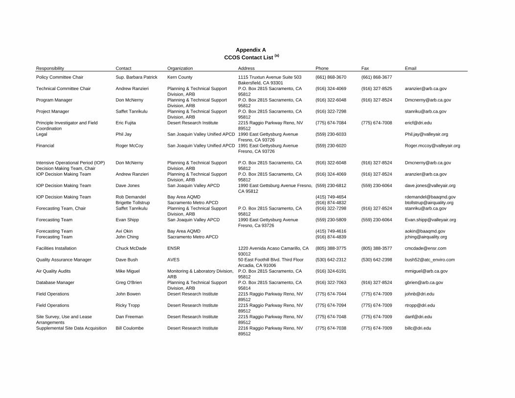
Appendix A CCOS Contact List (a)
Responsibility Contact Organization Address Phone Fax Email
Policy Committee Chair Sup. Barbara Patrick Kern County 1115 Truxtun Avenue Suite 503 Bakersfield, CA 93301
(661) 868-3670 (661) 868-3677
Technical Committee Chair Andrew Ranzieri Planning & Technical Support Division, ARB
P.O. Box 2815 Sacramento, CA 95812
(916) 324-4069 (916) 327-8525 [email protected]
Program Manager Don McNerny Planning & Technical Support Division, ARB
P.O. Box 2815 Sacramento, CA 95812
(916) 322-6048 (916) 327-8524 [email protected]
Project Manager Saffet Tanrikulu Planning & Technical Support Division, ARB
P.O. Box 2815 Sacramento, CA 95812
(916) 322-7298 [email protected]
Principle Investigator and Field Coordination
Eric Fujita Desert Research Institute 2215 Raggio Parkway Reno, NV 89512
(775) 674-7084 (775) 674-7008 [email protected]
Legal Phil Jay San Joaquin Valley Unified APCD 1990 East Gettysburg Avenue Fresno, CA 93726
(559) 230-6033 [email protected]
Financial Roger McCoy San Joaquin Valley Unified APCD 1991 East Gettysburg Avenue Fresno, CA 93726
(559) 230-6020 [email protected]
Intensive Operational Period (IOP) Decision Making Team, Chair
Don McNerny Planning & Technical Support Division, ARB
P.O. Box 2815 Sacramento, CA 95812
(916) 322-6048 (916) 327-8524 [email protected]
IOP Decision Making Team Andrew Ranzieri Planning & Technical Support Division, ARB
P.O. Box 2815 Sacramento, CA 95812
(916) 324-4069 (916) 327-8524 [email protected]
IOP Decision Making Team Dave Jones San Joaquin Valley APCD 1990 East Gettsburg Avenue Fresno, CA 95812
(559) 230-6812 (559) 230-6064 [email protected]
IOP Decision Making Team Rob Demandel Bay Area AQMD (415) 749-4654 [email protected] Tollstrup Sacramento Metro APCD (916) 874-4832 [email protected]
Forecasting Team, Chair Saffet Tanrikulu Planning & Technical Support Division, ARB
P.O. Box 2815 Sacramento, CA 95812
(916) 322-7298 (916) 327-8524 [email protected]
Forecasting Team Evan Shipp San Joaquin Valley APCD 1990 East Gettysburg Avenue Fresno, Ca 93726
(559) 230-5809 (559) 230-6064 [email protected]
Forecasting Team Avi Okin Bay Area AQMD (415) 749-4616 [email protected] Team John Ching Sacramento Metro APCD (916) 874-4839 [email protected]
Facilities Installation Chuck McDade ENSR 1220 Avenida Acaso Camarillo, CA 93012
(805) 388-3775 (805) 388-3577 [email protected]
Quality Assurance Manager Dave Bush AVES 50 East Foothill Blvd. Third Floor Arcadia, CA 91006
(530) 642-2312 (530) 642-2398 bush52@atc_enviro.com
Air Quality Audits Mike Miguel Monitoring & Laboratory Division, ARB
P.O. Box 2815 Sacramento, CA 95812
(916) 324-6191 [email protected]
Database Manager Greg O'Brien Planning & Technical Support Division, ARB
P.O. Box 2815 Sacramento, CA 95814
(916) 322-7063 (916) 327-8524 [email protected]
Field Operations John Bowen Desert Research Institute 2215 Raggio Parkway Reno, NV 89512
(775) 674-7044 (775) 674-7009 [email protected]
Field Operations Ricky Tropp Desert Research Institute 2215 Raggio Parkway Reno, NV 89512
(775) 674-7094 (775) 674-7009 [email protected]
Site Survey, Use and Lease Arrangements
Dan Freeman Desert Research Institute 2215 Raggio Parkway Reno, NV 89512
(775) 674-7048 (775) 674-7009 [email protected]
Supplemental Site Data Acquisition Bill Coulombe Desert Research Institute 2216 Raggio Parkway Reno, NV 89512
(775) 674-7038 (775) 674-7009 [email protected]
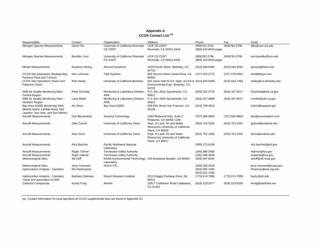
Appendix A CCOS Contact List (a)
Responsibility Contact Organization Address Phone Fax EmailNitrogen Species Measurements Denis Fitz University of California Riverside
CE-CERTUCR CE-CERT Riverside, CA 92521-0434
(909)781-5781 (909) 433-6534 pager
(909)781-5790 [email protected]
Nitrogen Species Measurements Bumiller, Kurt University of California Riverside CE-CERT
UCR CE-CERT Riverside, CA 92521-0435
(909)781-5796 (909) 433-6539 pager
(909)781-5790 [email protected]
Nitrate Measurements Susanne Hering Aerosol Dynamics 2329 Fourth Street Berkeley, CA 94710
(510) 649-9360 (510) 649-9260 [email protected]
CCOS Site Operations (Bodega Bay, Pacheco Pass and Turlock)
Don Lehrman T&B Systems 859 Second Street Santa Rosa, CA 95404
(707) 526-2775 (707) 579-5954 [email protected]
CCOS Site Operations (Sunol and Patterson Pass)
Rob Harley University of California Berkeley 631 Davis Hall #1710 Dept. of Civil & Environmental Engr. Berkeley, CA 94720
(510) 643-9168 (510) 642-7483 [email protected]
ARB Air Quality Monitoring Sites -Central Region
Peter Ouchida Monitoring & Laboratory Division, ARB
P.O. Box 2815 Sacramento, CA 95812
(916) 322-3719 (916) 327-8217 [email protected]
ARB Air Quality Monitoring Sites - Northern Region
Larry Molek Monitoring & Laboratory Division, ARB
P.O. Box 2815 Sacramento, CA 95812
(916) 327-4889 (916) 327-8217 [email protected]
Bay Area AQMD Monitoring Sites (Bethel Island, Lambie Road, San Leandro, San Jose, and San Martin)
Avi Oken Bay Area AQMD 939 Ellis Street San Franciso, CA 94109
(510) 749-4616 [email protected]
Aircraft Measurements Don Blumenthal Sonoma Technology 1360 Redwood Way, Suite C Petaluma, CA 94954-1169
(707) 665-9900 (707) 665-9800 [email protected]
Aircraft Measurements John Carroll University of California, Davis Dept. of Land, Air and Water Resources University of California Davis, CA 95616
(916) 752-3245 (916) 752-1552 [email protected]
Aircraft Measurements Alan Dixon University of California, Davis Dept. of Land, Air and Water Resources University of California Davis, CA 95617
(916) 752-1459 (916) 752-1552 [email protected]
Aircraft Measurements Rich Barchet Pacific Northwest National Laboratory
(509) 372-6158 [email protected]
Aircraft Measurements Roger Tanner Tennessee Valley Authority (256) 386-2958 [email protected] Measurements Raph Valente Tennessee Valley Authority (256) 386-3649 [email protected] Sites Bill Neff NOAA Environmental Technology
Laboratory325 Broadway Boulder, CA 80303 (303) 497-6265 [email protected]
Meteorological Sites Jerry Crescenti NOAA ATL (208) 526-2328 [email protected] Analysis - Canisters Rei Rasmussen (503) 690-1094
(503) [email protected]
Hydrocarbon Analysis - Canisters, Tenax and automated GC/MS
Barbara Zielinska Desert Research Institute 2215 Raggio Parkway Reno, NV 89512
(775) 674-7066 (775) 674-7008 [email protected]
Carbonyl Compounds Kochy Fung AtmAA 23917 Craftsman Road Calabasas, CA 91302
(818) 223-3277 (818) 223-8250 [email protected]
(a) Contact information for local operators at CCOS supplemental sites are found in Appendix D1
APPENDIX B
AIR QUALITY MONITORING SITES INCENTRAL AND NORTHERN CALIFORNIA

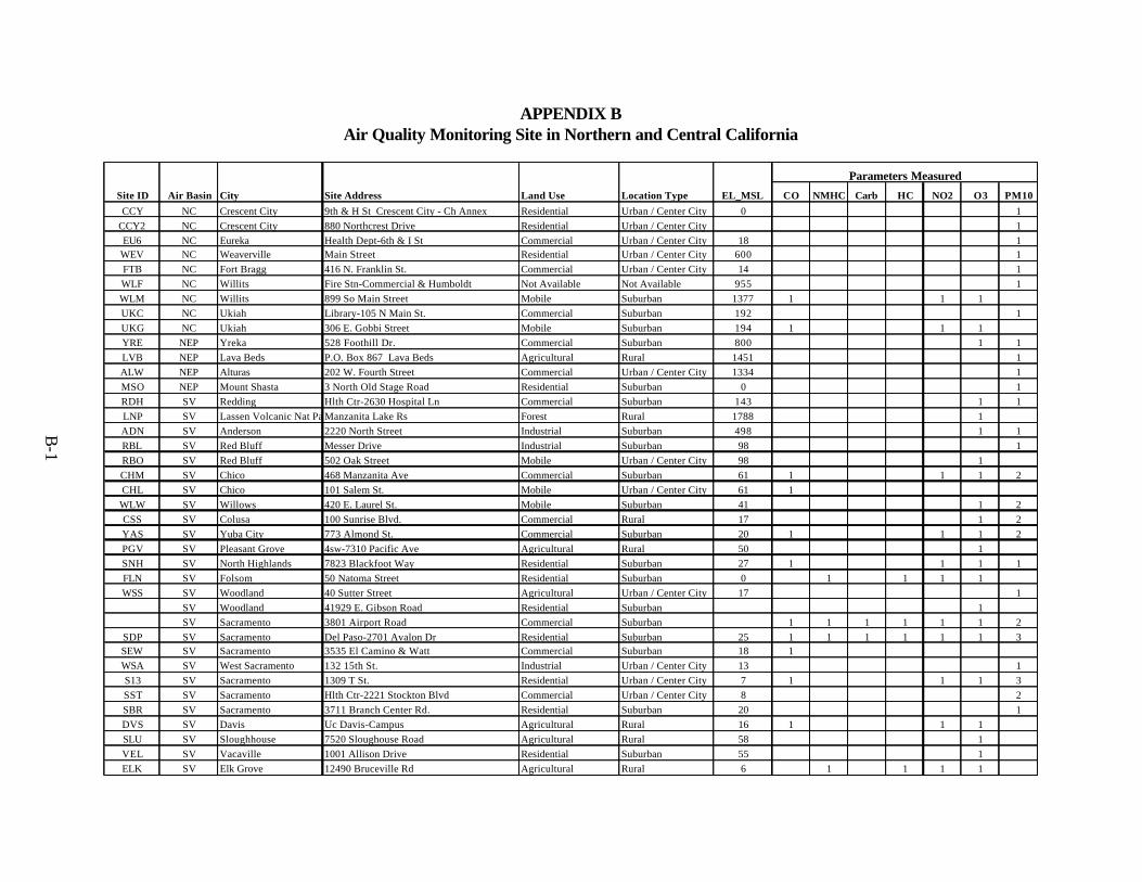
B-1
APPENDIX BAir Quality Monitoring Site in Northern and Central California
Parameters Measured
Site ID Air Basin City Site Address Land Use Location Type EL_MSL CO NMHC Carb HC NO2 O3 PM10
CCY NC Crescent City 9th & H St Crescent City - Ch Annex Residential Urban / Center City 0 1
CCY2 NC Crescent City 880 Northcrest Drive Residential Urban / Center City 1
EU6 NC Eureka Health Dept-6th & I St Commercial Urban / Center City 18 1WEV NC Weaverville Main Street Residential Urban / Center City 600 1
FTB NC Fort Bragg 416 N. Franklin St. Commercial Urban / Center City 14 1
WLF NC Willits Fire Stn-Commercial & Humboldt Not Available Not Available 955 1
WLM NC Willits 899 So Main Street Mobile Suburban 1377 1 1 1
UKC NC Ukiah Library-105 N Main St. Commercial Suburban 192 1
UKG NC Ukiah 306 E. Gobbi Street Mobile Suburban 194 1 1 1
YRE NEP Yreka 528 Foothill Dr. Commercial Suburban 800 1 1
LVB NEP Lava Beds P.O. Box 867 Lava Beds Agricultural Rural 1451 1
ALW NEP Alturas 202 W. Fourth Street Commercial Urban / Center City 1334 1
MSO NEP Mount Shasta 3 North Old Stage Road Residential Suburban 0 1
RDH SV Redding Hlth Ctr-2630 Hospital Ln Commercial Suburban 143 1 1
LNP SV Lassen Volcanic Nat ParkManzanita Lake Rs Forest Rural 1788 1
ADN SV Anderson 2220 North Street Industrial Suburban 498 1 1
RBL SV Red Bluff Messer Drive Industrial Suburban 98 1
RBO SV Red Bluff 502 Oak Street Mobile Urban / Center City 98 1
CHM SV Chico 468 Manzanita Ave Commercial Suburban 61 1 1 1 2
CHL SV Chico 101 Salem St. Mobile Urban / Center City 61 1
WLW SV Willows 420 E. Laurel St. Mobile Suburban 41 1 2
CSS SV Colusa 100 Sunrise Blvd. Commercial Rural 17 1 2
YAS SV Yuba City 773 Almond St. Commercial Suburban 20 1 1 1 2
PGV SV Pleasant Grove 4sw-7310 Pacific Ave Agricultural Rural 50 1
SNH SV North Highlands 7823 Blackfoot Way Residential Suburban 27 1 1 1 1
FLN SV Folsom 50 Natoma Street Residential Suburban 0 1 1 1 1
WSS SV Woodland 40 Sutter Street Agricultural Urban / Center City 17 1
SV Woodland 41929 E. Gibson Road Residential Suburban 1
SV Sacramento 3801 Airport Road Commercial Suburban 1 1 1 1 1 1 2
SDP SV Sacramento Del Paso-2701 Avalon Dr Residential Suburban 25 1 1 1 1 1 1 3SEW SV Sacramento 3535 El Camino & Watt Commercial Suburban 18 1
WSA SV West Sacramento 132 15th St. Industrial Urban / Center City 13 1
S13 SV Sacramento 1309 T St. Residential Urban / Center City 7 1 1 1 3
SST SV Sacramento Hlth Ctr-2221 Stockton Blvd Commercial Urban / Center City 8 2
SBR SV Sacramento 3711 Branch Center Rd. Residential Suburban 20 1
DVS SV Davis Uc Davis-Campus Agricultural Rural 16 1 1 1
SLU SV Sloughhouse 7520 Sloughouse Road Agricultural Rural 58 1
VEL SV Vacaville 1001 Allison Drive Residential Suburban 55 1
ELK SV Elk Grove 12490 Bruceville Rd Agricultural Rural 6 1 1 1 1
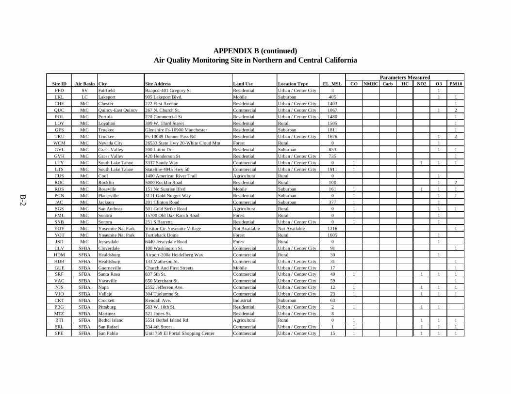
B-2
APPENDIX B (continued)Air Quality Monitoring Site in Northern and Central California
Parameters MeasuredSite ID Air Basin City Site Address Land Use Location Type EL_MSL CO NMHC Carb HC NO2 O3 PM10
FFD SV Fairfield Baapcd-401 Gregory St Residential Urban / Center City 3 1
LKL LC Lakeport 905 Lakeport Blvd. Mobile Suburban 405 1 1
CHE MtC Chester 222 First Avenue Residential Urban / Center City 1403 1
QUC MtC Quincy-East Quincy 267 N. Church St. Commercial Urban / Center City 1067 1 2
POL MtC Portola 220 Commercial St Residential Urban / Center City 1480 1
LOY MtC Loyalton 309 W. Third Street Residential Rural 1505 1
GFS MtC Truckee Glenshire Fs-10900 Manchester Residential Suburban 1811 1
TRU MtC Truckee Fs-10049 Donner Pass Rd Residential Urban / Center City 1676 1 2
WCM MtC Nevada City 26533 State Hwy 20-White Cloud Mtn Forest Rural 0 1
GVL MtC Grass Valley 200 Litton Dr. Residential Suburban 853 1 1
GVH MtC Grass Valley 420 Henderson St Residential Urban / Center City 735 1
LTY MtC South Lake Tahoe 3337 Sandy Way Commercial Urban / Center City 0 1 1 1 1
LTS MtC South Lake Tahoe Stateline-4045 Hwy 50 Commercial Urban / Center City 1911 1
CUS MtC Cool 1400 American River Trail Agricultural Rural 0 1
ROC MtC Rocklin 5000 Rocklin Road Residential Rural 100 1 2
ROS MtC Roseville 151 No Sunrise Blvd Mobile Suburban 161 1 1 1 1
PGN MtC Placerville 3111 Gold Nugget Way Residential Suburban 0 1 1 1
JAC MtC Jackson 201 Clinton Road Commercial Suburban 377 1 1
SGS MtC San Andreas 501 Gold Strike Road Agricultural Rural 0 1 1 1
FML MtC Sonora 15700 Old Oak Ranch Road Forest Rural 0 1
SNB MtC Sonora 251 S Barretta Residential Urban / Center City 0 1 1
YOY MtC Yosemite Nat Park Visitor Ctr-Yosemite Village Not Available Not Available 1216 1
YOT MtC Yosemite Nat Park Turtleback Dome Forest Rural 1605 1
JSD MtC Jerseydale 6440 Jerseydale Road Forest Rural 0 1
CLV SFBA Cloverdale 100 Washington St. Commercial Urban / Center City 91 1
HDM SFBA Healdsburg Airport-200a Heidelberg Way Commercial Rural 30 1
HDB SFBA Healdsburg 133 Matheson St. Commercial Urban / Center City 31 1
GUE SFBA Guerneville Church And First Streets Mobile Urban / Center City 17 1SRF SFBA Santa Rosa 837 5th St. Commercial Urban / Center City 49 1 1 1 1
VAC SFBA Vacaville 650 Merchant St. Commercial Urban / Center City 59 1
NJS SFBA Napa 2552 Jefferson Ave. Commercial Urban / Center City 12 1 1 1 1
VJO SFBA Vallejo 304 Tuolumne St. Commercial Urban / Center City 23 1 1 1 1
CKT SFBA Crockett Kendall Ave. Industrial Suburban 63
PBG SFBA Pittsburg 583 W. 10th St. Residential Urban / Center City 2 1 1 1
MTZ SFBA Martinez 521 Jones St. Residential Urban / Center City 8
BTI SFBA Bethel Island 5551 Bethel Island Rd Agricultural Rural 0 1 1 1 1
SRL SFBA San Rafael 534 4th Street Commercial Urban / Center City 1 1 1 1 1
SPE SFBA San Pablo Unit 759 El Portal Shopping Center Commercial Urban / Center City 15 1 1 1 1
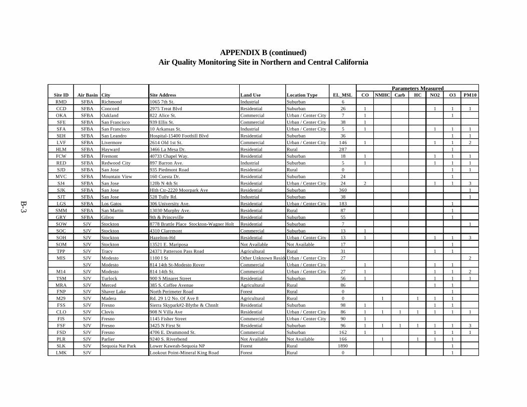
B-3
APPENDIX B (continued)Air Quality Monitoring Site in Northern and Central California
Parameters MeasuredSite ID Air Basin City Site Address Land Use Location Type EL_MSL CO NMHC Carb HC NO2 O3 PM10RMD SFBA Richmond 1065 7th St. Industrial Suburban 6
CCD SFBA Concord 2975 Treat Blvd Residential Suburban 26 1 1 1 1
OKA SFBA Oakland 822 Alice St. Commercial Urban / Center City 7 1 1
SFE SFBA San Francisco 939 Ellis St. Commercial Urban / Center City 38 1
SFA SFBA San Francisco 10 Arkansas St. Industrial Urban / Center City 5 1 1 1 1
SEH SFBA San Leandro Hospital-15400 Foothill Blvd Residential Suburban 36 1 1
LVF SFBA Livermore 2614 Old 1st St. Commercial Urban / Center City 146 1 1 1 2
HLM SFBA Hayward 3466 La Mesa Dr. Residential Rural 287 1
FCW SFBA Fremont 40733 Chapel Way. Residential Suburban 18 1 1 1 1
RED SFBA Redwood City 897 Barron Ave. Industrial Suburban 5 1 1 1 1
SJD SFBA San Jose 935 Piedmont Road Residential Rural 0 1 1
MVC SFBA Mountain View 160 Cuesta Dr. Residential Suburban 24 1
SJ4 SFBA San Jose 120b N 4th St Residential Urban / Center City 24 2 1 1 3
SJK SFBA San Jose Hlth Ctr-2220 Moorpark Ave Residential Suburban 360 1
SJT SFBA San Jose 528 Tully Rd. Industrial Suburban 38 1
LGS SFBA Los Gatos 306 University Ave. Residential Urban / Center City 183 1
SMM SFBA San Martin 13030 Murphy Ave. Residential Rural 87 1
GRY SFBA Gilroy 9th & Princeville Residential Suburban 55 1
SOW SJV Stockton 8778 Brattle Place Stockton-Wagner Holt Residential Suburban 7 1
SOC SJV Stockton 4310 Claremont Commercial Suburban 13 1
SOH SJV Stockton Hazelton-Hd Residential Urban / Center City 13 1 1 1 3
SOM SJV Stockton 13521 E. Mariposa Not Available Not Available 17 1
TPP SJV Tracy 24371 Patterson Pass Road Agricultural Rural 31 1 1
MIS SJV Modesto 1100 I St Other Unknown ResidentialUrban / Center City 27 2
SJV Modesto 814 14th St-Modesto Rover Commercial Urban / Center City 1 1 1
M14 SJV Modesto 814 14th St. Commercial Urban / Center City 27 1 1 1 2
TSM SJV Turlock 900 S Minaret Street Residential Suburban 56 1 1 1 1
MRA SJV Merced 385 S. Coffee Avenue Agricultural Rural 86 1 1FNP SJV Shaver Lake North Perimeter Road Forest Rural 0 1
M29 SJV Madera Rd. 29 1/2 No. Of Ave 8 Agricultural Rural 0 1 1 1 1
FSS SJV Fresno Sierra Skypark#2-Blythe & Chnnlt Residential Suburban 98 1 1 1
CLO SJV Clovis 908 N Villa Ave Residential Urban / Center City 86 1 1 1 1 1 1 1
FIS SJV Fresno 1145 Fisher Street Commercial Urban / Center City 90 1
FSF SJV Fresno 3425 N First St Residential Suburban 96 1 1 1 1 1 1 3
FSD SJV Fresno 4706 E. Drummond St. Commercial Suburban 162 1 1 1 1
PLR SJV Parlier 9240 S. Riverbend Not Available Not Available 166 1 1 1 1
SLK SJV Sequoia Nat Park Lower Kaweah-Sequoia NP Forest Rural 1890 1
LMK SJV Lookout Point-Mineral King Road Forest Rural 0 1
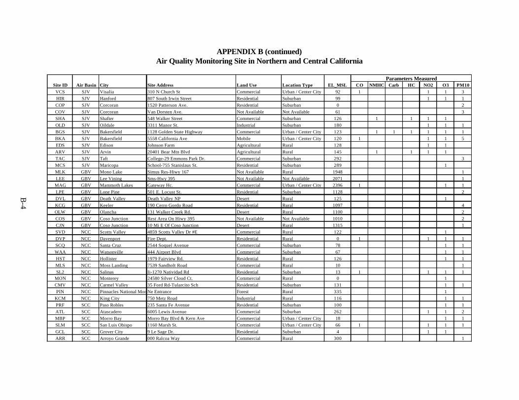
B-4
APPENDIX B (continued)Air Quality Monitoring Site in Northern and Central California
Parameters MeasuredSite ID Air Basin City Site Address Land Use Location Type EL_MSL CO NMHC Carb HC NO2 O3 PM10
VCS SJV Visalia 310 N Church St Commercial Urban / Center City 92 1 1 1 3
HIR SJV Hanford 807 South Irwin Street Residential Suburban 99 1 1 1
COP SJV Corcoran 1520 Patterson Ave. Residential Suburban 0 2
COV SJV Corcoran Van Dorsten Ave. Not Available Not Available 61 3
SHA SJV Shafter 548 Walker Street Commercial Suburban 126 1 1 1 1
OLD SJV Oildale 3311 Manor St. Industrial Suburban 180 1 1 1
BGS SJV Bakersfield 1128 Golden State Highway Commercial Urban / Center City 123 1 1 1 1 1 1
BKA SJV Bakersfield 5558 California Ave Mobile Urban / Center City 120 1 1 1 5
EDS SJV Edison Johnson Farm Agricultural Rural 128 1 1
ARV SJV Arvin 20401 Bear Mtn Blvd Agricultural Rural 145 1 1 1 1
TAC SJV Taft College-29 Emmons Park Dr. Commercial Suburban 292 3
MCS SJV Maricopa School-755 Stanislaus St. Residential Suburban 289 1
MLK GBV Mono Lake Simus Res-Hiwy 167 Not Available Rural 1948 1
LEE GBV Lee Vining Sms-Hwy 395 Not Available Not Available 2071 1
MAG GBV Mammoth Lakes Gateway Hc. Commercial Urban / Center City 2396 1 1 1
LPE GBV Lone Pine 501 E. Locust St. Residential Suburban 1128 2
DVL GBV Death Valley Death Valley NP Desert Rural 125 1
KCG GBV Keeler 190 Cerro Gordo Road Residential Rural 1097 4
OLW GBV Olancha 131 Walker Creek Rd. Desert Rural 1100 2
COS GBV Coso Junction Rest Area On Hiwy 395 Not Available Not Available 1010 2
CJN GBV Coso Junction 10 Mi E Of Coso Junction Desert Rural 1315 1
SVD NCC Scotts Valley 4859 Scotts Valley Dr #E Commercial Rural 122 1
DVP NCC Davenport Fire Dept. Residential Rural 0 1 1 1 1
SCQ NCC Santa Cruz 2544 Soquel Avenue Commercial Suburban 78 1 1
WAA NCC Watsonville 444 Airport Blvd Commercial Suburban 67 1 1
HST NCC Hollister 1979 Fairview Rd. Residential Rural 126 1 1
MLS NCC Moss Landing 7539 Sandholt Road Commercial Rural 10 1
SL2 NCC Salinas Ii-1270 Natividad Rd Residential Suburban 13 1 1 1 1MON NCC Monterey 24580 Silver Cloud Ct. Commercial Rural 0 1
CMV NCC Carmel Valley 35 Ford Rd-Tularcito Sch Residential Suburban 131 1 1
PIN NCC Pinnacles National MonumentNe Entrance Forest Rural 335 1
KCM NCC King City 750 Metz Road Industrial Rural 116 1 1
PRF SCC Paso Robles 235 Santa Fe Avenue Residential Suburban 100 1 1
ATL SCC Atascadero 6005 Lewis Avenue Commercial Suburban 262 1 1 2
MBP SCC Morro Bay Morro Bay Blvd & Kern Ave Commercial Urban / Center City 18 1 1
SLM SCC San Luis Obispo 1160 Marsh St. Commercial Urban / Center City 66 1 1 1 1
GCL SCC Grover City 9 Le Sage Dr. Residential Suburban 4 1 1
ARR SCC Arroyo Grande 000 Ralcoa Way Commercial Rural 300 1
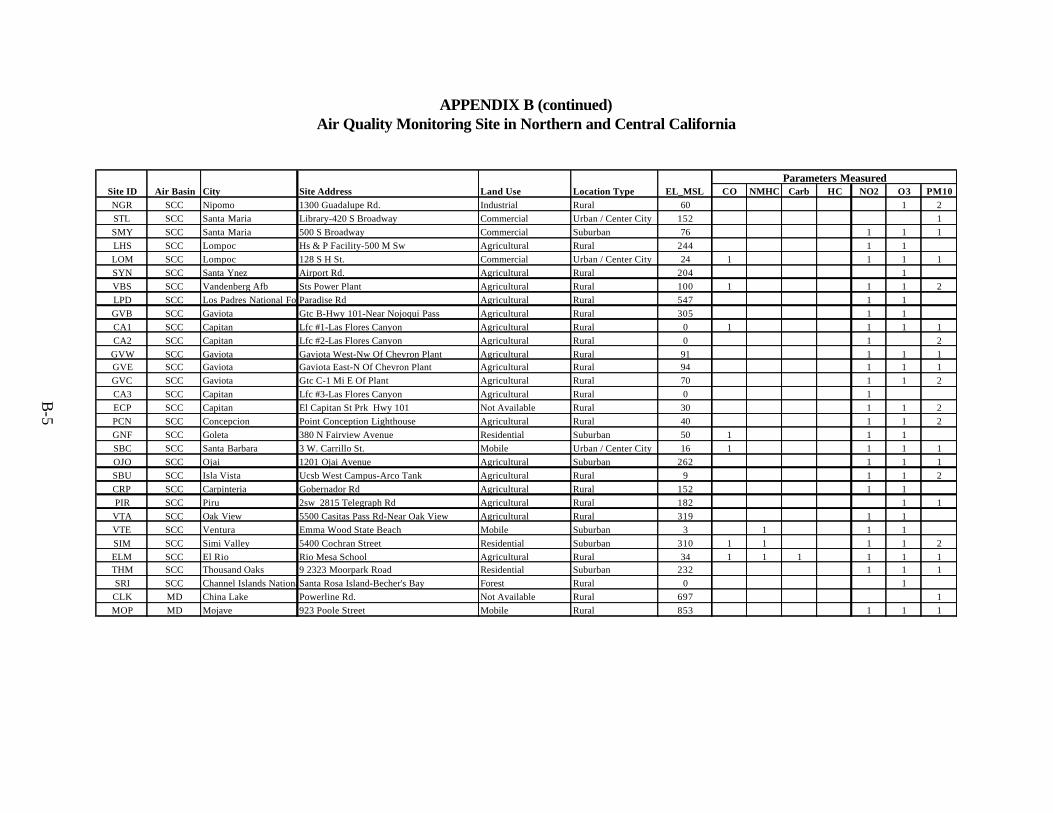
B-5
APPENDIX B (continued)Air Quality Monitoring Site in Northern and Central California
Parameters MeasuredSite ID Air Basin City Site Address Land Use Location Type EL_MSL CO NMHC Carb HC NO2 O3 PM10NGR SCC Nipomo 1300 Guadalupe Rd. Industrial Rural 60 1 2
STL SCC Santa Maria Library-420 S Broadway Commercial Urban / Center City 152 1
SMY SCC Santa Maria 500 S Broadway Commercial Suburban 76 1 1 1
LHS SCC Lompoc Hs & P Facility-500 M Sw Agricultural Rural 244 1 1
LOM SCC Lompoc 128 S H St. Commercial Urban / Center City 24 1 1 1 1
SYN SCC Santa Ynez Airport Rd. Agricultural Rural 204 1
VBS SCC Vandenberg Afb Sts Power Plant Agricultural Rural 100 1 1 1 2
LPD SCC Los Padres National ForestParadise Rd Agricultural Rural 547 1 1
GVB SCC Gaviota Gtc B-Hwy 101-Near Nojoqui Pass Agricultural Rural 305 1 1
CA1 SCC Capitan Lfc #1-Las Flores Canyon Agricultural Rural 0 1 1 1 1
CA2 SCC Capitan Lfc #2-Las Flores Canyon Agricultural Rural 0 1 2
GVW SCC Gaviota Gaviota West-Nw Of Chevron Plant Agricultural Rural 91 1 1 1GVE SCC Gaviota Gaviota East-N Of Chevron Plant Agricultural Rural 94 1 1 1
GVC SCC Gaviota Gtc C-1 Mi E Of Plant Agricultural Rural 70 1 1 2
CA3 SCC Capitan Lfc #3-Las Flores Canyon Agricultural Rural 0 1
ECP SCC Capitan El Capitan St Prk Hwy 101 Not Available Rural 30 1 1 2
PCN SCC Concepcion Point Conception Lighthouse Agricultural Rural 40 1 1 2
GNF SCC Goleta 380 N Fairview Avenue Residential Suburban 50 1 1 1
SBC SCC Santa Barbara 3 W. Carrillo St. Mobile Urban / Center City 16 1 1 1 1
OJO SCC Ojai 1201 Ojai Avenue Agricultural Suburban 262 1 1 1
SBU SCC Isla Vista Ucsb West Campus-Arco Tank Agricultural Rural 9 1 1 2
CRP SCC Carpinteria Gobernador Rd Agricultural Rural 152 1 1
PIR SCC Piru 2sw 2815 Telegraph Rd Agricultural Rural 182 1 1
VTA SCC Oak View 5500 Casitas Pass Rd-Near Oak View Agricultural Rural 319 1 1
VTE SCC Ventura Emma Wood State Beach Mobile Suburban 3 1 1 1
SIM SCC Simi Valley 5400 Cochran Street Residential Suburban 310 1 1 1 1 2
ELM SCC El Rio Rio Mesa School Agricultural Rural 34 1 1 1 1 1 1THM SCC Thousand Oaks 9 2323 Moorpark Road Residential Suburban 232 1 1 1
SRI SCC Channel Islands National ParkSanta Rosa Island-Becher's Bay Forest Rural 0 1
CLK MD China Lake Powerline Rd. Not Available Rural 697 1
MOP MD Mojave 923 Poole Street Mobile Rural 853 1 1 1
APPENDIX C
MEASUREMENT METHODS

C-1
C. MEASUREMENT METHODS
Field monitoring includes continuous measurements over several months and intensivestudies that are performed on a forecast basis during selected periods when episodes are mostlikely to occur. The continuous measurements are made in order to assess the representativenessof the intensive study days, to provide information on the meteorology and air quality conditions ondays leading up to the episodes, and to assess the meteorological regimes and transport patternswhich lead to ozone episodes. The intensive study components are designed to provide a detailedaerometric database which, along with the emission estimates and continuous monitoring data, canbe used to improve our understanding of the causes of pollutant episodes in the study region and toprovide data for input to the models and for model evaluation. This section describes the optionsfor continuous and intensive air quality and meteorological measurements (surface and aloft) to bemade during CCOS.
C.1 Surface Meteorology
The types of surface meteorological measurements needed for this study includemeasurements of wind speed, wind direction, and temperature. Measurements of humidity,pressure, visibility, solar radiation, and ultraviolet radiation are also available at some sites.Within the study area (modeling domain), these measurements are provided by several existingnetworks of sites operated by several organizations including:
• Surface Airways Observations sites from the National Weather Service (NWS),operating in conjunction with the Federal Aviation Administration
• California Irrigation Management Information System sites from the CaliforniaDepartment of Agriculture
• Remote Automated Weather Station sites from the Bureau of Land Management,California Department of Forestry, National Park Service, and U.S. Forest Service
• APCD/AQMD Aerometric Monitoring Station sites from the Bay Area AQMD, KernCounty APCD, San Joaquin Valley Unified Control District, Santa Barbara APCD,Ventura County APCD, Mojave Desert AQMD, and California Air Resources Board
• Military installations
• Private companies
• Public organizations such as universities
C.1.1 Surface Wind Speed and Direction
Wind speeds are measured with anemometers at 10 m above ground to minimize the effectsof nearby structures and vegetation. Anemometers, both cup and propeller type, work on theprincipal that the rate of rotation about a vertical or horizontal shaft is proportional to the speed ofthe air flow past the sensor. Anemometers used for scientific monitoring should have a quick
C-2
response to changes in wind speed as well as a low threshold for rotation for conditions of verylight winds. Acceptable precision levels for anemometers are ±0.5 m/s for most air qualitystudies (e.g., Thullier et al., 1993).
Wind direction measurements are made with wind vanes that orient themselves with thedirection of the wind. High quality bearings are used for sensitivity and direction is resolved withan internal potentiometer that has a reference location of zero which must be physically alignedwith true north when in position on the tower. The position of true north is determined with asensitive compass or solar reference and the north position of the wind vane is then aligned in thisdirection. Care must be taken in the alignment procedure or in subsequent resolution of the winddirection vectors to account for the magnetic declination at the observation site.
Averaging can be done over intervals of a few points to the entire data record. Theinterval must be chosen with respect to the phenomena being observed. As shorter averagingintervals are chosen, periodic motion may be revealed when the period is significantly greater thanthe averaging period. The averaging process attenuates small-scale fluctuations due to turbulence.The averaging interval must contain sufficient data points to constitute a reasonable average,eliminating the small scale turbulent fluctuations and instrument derived errors such as responsesensitivity and anemometer run-up and run-down. Five minutes is a reasonable compromisebetween the need to acquire a statistically valid number of samples and the nature of phenomenasuch as wind gusts and dispersion.
The time average of horizontal wind direction standard deviation (σθ) can be calculated asfrom one second observations over a period of 5 minutes or less (Greeley and Iversen, 1985).This minimizes the influence of the wind flow which may be non-stationary in both speed anddirection over longer averaging periods.
C.1.2 Surface Relative Humidity
Humidity indicates the amount of water vapor in the air. The most common reference forthis property of the air is the relative humidity (RH), the ratio of the amount of water vaporactually in the air to the amount the air could hold at a given temperature and pressure, that is, theratio of the actual to the saturated vapor pressure.
Accurate measurements at high RH (>85%) is important to atmospheric transformationsand to visibility reduction. An accuracy of 2-3% RH is needed to adequately estimate aerosolproperties. A 2-3% accuracy for RH over the 90-100% RH is attainable by several RH sensors(e.g. Vaisala, Rotronics) and corresponds to ±0.5°C when expressed as dewpoint temperature.Motor-aspirated radiation shields ensure adequate ventilation and exposure rates (U.S. EPA,1989).
C.1.3 Surface Temperature
Equivalent resistance temperature detectors (RTD (e.g., Vaisala, Rotronics, Climatronics,Campbell Scientific, etc.) are used at the meteorological sites. Motor-aspirated radiation shieldsensure adequate ventilation and exposure rates, according to U.S. EPA quality assurancerequirements (U.S. EPA, 1989). The accuracy (~0.15-0.5 °C) and functional precision (0.1°C) of
C-3
these sensors are sufficiently good and they can be used to infer lapse rates and thus stability (e.g.,estimates of delta-T) when several sensors are used on a tower. Temperature sensors arenormally located at 5 m above ground level. Table 10.1-1 presents specifications for the Vaisalaand Campbell Scientific (CV) temperature (�C) and relative humidity (%) sensors
C.1.4 Surface Pressure
Pressure is routinely measured by the National Weather Service in terms of altimetersetting or sea level pressure. The altimeter setting is the pressure value to which an aircraftaltimeter scale is set so it will indicate the altitude above mean-sea-level of the aircraft on theground at the location the pressure value was determined. The sea level pressure is theatmospheric pressure at mean sea level. It is either measured directly or obtained by the empiricalreduction of station pressure to sea level. When the earth's surface is above sea level, it isassumed that the atmosphere extends to sea level below the station and that the properties of thefictitious air column are related to conditions observed at the station.
C.1.5 Solar Radiation
Solar radiation sensors are operated at several existing ARB sites throughout the region. Themeasurements employ a solar pyranometer that collects direct solar beam and diffuse sky radiationpassing though a horizontal beam.
C.2 Upper-Air Wind Speed, Wind Direction, and Temperature
The types of upper-air meteorological measurements needed include wind speed, winddirection, temperature, and mixing height. Measurements of humidity are also useful where theyare available at some sites. A comprehensive discussion of the accuracy and methodology ofupper air measurements is provided in the SJVAQS/AUSPEX Meteorological Field MeasurementProgram report (Thuillier, 1994).
C.2.1 Radar Wind Profilers
Radar wind profilers (RWPs) provide continuous remote measurements of wind speed anddirection to altitudes of ~3 km AGL. The profilers emit short pulses of generally 915 MHzelectromagnetic radiation which scatter off inhomogeneities in the index of refraction of an airmass. By emitting energy directionally in three orthogonal components, the received scatteredradiation provides estimates of wind speed and direction. Because of the finite length of theemitted pulse train, vertical resolution is limited to approximately 100 m. Echoes received duringthe detector downtime cannot be processed and this raises the threshold height to approximately100 m above ground level. The typical five-degree beam width also limits the resolution of winddirection in a height dependent manner. There are general trade-offs between maximum range andvertical resolution and between averaging time and accuracy.
Radar wind profiler data are generally reported as 15-minute up to hourly averaged dataand are representative of a three-dimensional cell. Because wind vectors may vary significantlyover the course of an hour, the near-instantaneous radiosonde measurements may not compare wellwith radar wind profiler measurements on a case-by-case basis. However, if radiosondes and
C-4
wind profilers are deployed in areas with similar winds, the statistical distribution of winds maybe expected to be reasonably similar. The RWP is highly sensitive to stray electromagneticsignals and stationary or solid objects in the beam paths or their side lobes. Thus, it should besited away from large objects such as buildings and trees and away from frequent overflights byaircraft.
C.2.2 Radio-Acoustic Sounding Systems (RASS)
Temperature aloft up to 500-700 m can be characterized using a RASS. The RASSessentially uses collocated radio wave and acoustic sources such that radio waves are scatteredoff the acoustic wavefronts. The propagation velocity of the acoustic wave fronts is thenmeasured, which can be related to the (virtual) temperature of the air. This effort could install oneradar profiler with RASS at critical locations along major transport paths, such as mountain passesor the coastal shoreline, for example, near Cajon and Banning Passes and along the downwindshorelines in San Diego and Santa Barbara. There is considerably less accuracy in the RASStemperature profiles compared to the those obtainable from tethersonde measurements, particularlyin areas of complex terrain where radar side lobes may present a problem. However, the RASStemperature data may be compared to QA radiosonde or tethersonde temperature data because thevirtual temperature can also be calculated from the sonde measurements of ambient temperature,dew point or relative humidity, and pressure. A favorable comparison under representativeconditions would increase confidence in the RASS data at these sites.
C.2.3 Acoustic Sounders (Sodars)
The sodar uses an observational process that is similar to the RWP except that the sodaruses pulses of acoustic instead of electromagnetic energy. The sodar then detects returned acousticenergy scattered from turbulent density fluctuation (instead of index of refraction fluctuations). Itprovides hourly averaged wind speed and direction up to a 500-600 m maximum range with athreshold height of approximately 50-60 m. The sodar can operate routinely with little or no on-site care, but compared to radiosondes it does not measure humidity, and the equipment isexpensive. The sodar is highly sensitive to extraneous sources of sound. Thus, it should be sitedaway from substantial and continuous noise sources such as heavily traveled roads. The sodaracoustic emissions are audible and may disturb nearby residents, which can be a sitingdisadvantage compared with the RWP. With the lower vertical range, sodars should be deployedin areas of lower expected mixing heights, such as in marine layers.
C.2.4 Radiosondes
Upper-air wind speed, wind direction, and temperature can be collected by in-situ systemsor by remote sensing instruments. The most commonly used in-situ systems rely on a balloon-borne sensor (radiosonde), carried aloft by a freely ascending weather balloon to measureatmospheric pressure, temperature, and moisture (relative humidity or wet bulb temperature).These thermodynamic variables are used to compute the altitude of the balloon. Wind speed anddirection aloft are determined by measuring the position of the balloon as it ascends. The positiondata can be obtained by tracking the balloon from a fixed ground station using radio directionfinding techniques (RDF) or optical tracking, or they can be obtained using one of the radionavigation (NAVAID) networks, such as loran or Global Positioning System (GPS). By measuring
C-5
the position of the balloon with respect to time and altitude, horizontal wind vectors can becomputed that represent the layer-averaged wind speed and wind direction for successive layers.Balloons can also measure relative humidity, which is not detected by proven remote sensingmethods.
The vertical resolution of the wind data is typically 50-200 m (depending on altitude andthe type of sounding system used), and the range is from about 100 m above ground level (AGL) toaltitudes as high as 10,000 m altitude or higher. Radiosondes provide wind data that are averagedover short vertical distances and are thus nearly instantaneous measurements at a particularlocation. Although the radiosonde directly measures temperature and humidity during the shortballoon flight, it is only a "snapshot" at each level of the atmosphere. As the radiosonde rises, it istransported downwind, so measurements are not made above a fixed location, as within a windprofiler, for example.
For air pollution studies such as this, balloon sounding systems can provide relativelycomplete profiles of winds, temperature, and moisture in the boundary layer and lowertroposphere. Balloon soundings usually can be made two to eight times per day on selectedsampling days within reasonable budget contraints, but they are not cost-effective for long-termmonitoring.
C.2.5 Sonic Anemometers
Sonic anemometers deployed at surface sites would provide estimates of turbulent fluxesfor the modeling effort. The variations in sound propagation over a short (30 cm) path aretypically sampled at 10 Hz, providing an estimate of turbulent fluctuations over that path. One-dimensional sonic anemometers measure vertical turbulent flux, while three-dimensional sonicanemometers include turbulent fluxes in the two horizontal dimensions. These data provideboundary layer characterization, representative of the type of terrain over which the measurementis taken. Urban effects could be better incorporated in the mesoscale model. The measurementcould provide better dispersion estimates for models run in the data assimilation mode, andprovide real-world measurements against which model estimates of turbulent flux are compared.
C.3 Routine Surface Air Quality
The California Air Resources Board and local air pollution control districts operate anetwork of sampling sites that measure ambient pollutant levels. This network consists of threetypes of surface air quality monitoring stations. The National Air Monitoring Stations (NAMS)were established to ensure a long term national network for urban area-oriented ambientmonitoring and to provide a systematic, consistent database for air quality comparisons and trendanalysis. The State and Local Air Monitoring Stations (SLAMS) allow state and localgovernments to develop networks tailored to their immediate monitoring needs. Special purposemonitors (SPM) fulfill very specific or short-term monitoring goals. SPMs are typically used assource-oriented monitors rather than monitors which reflect the overall urban air quality. Datafrom all three types are submitted by state and local agencies to EPA’s Aerometric InformationRetrieval System (AIRS), which serves as the national repository for air quality, meteorologicaland emissions data.
C-6
Under Title I, Section 182, of the 1990 Amendments to the Federal Clean Air Act, the EPAproposed a rule to revise the current ambient air quality surveillance regulations. The rulerequires implementing a national network of enhanced ambient air monitoring stations (FederalRegister, 1993). States with areas classified as serious, severe, or extreme for ozonenonattainment are required to establish photochemical assessment monitoring stations (PAMS) aspart of their State Implementation Plan (SIP). In the CCOS area, PAMS are required inSacramento, Fresno and Bakerfield metropolitan areas. Each station measures speciatedhydrocarbons and carbonyl compounds, ozone, oxides of nitrogen, and surface meteorologicaldata. Additionally, each area must monitor upper air meteorology at one representative site. Theprogram was phased in over a five-year schedule, beginning in 1994, at a rate of at least onestation per area per year. Intended applications for the PAMS database include ozone andprecursor trends, emission inventory reconciliation and verification, population exposure analyses,photochemical modeling support, and control strategy evaluation.
There are 185 active monitoring stations in northern and central California. Table A.1-2contains a list of the monitoring sites and the air quality parameters measured at each site. Of theactive sites, 130 measure ozone and 76 measure NOX. Carbon monoxide and total hydrocarbonsare measured at 57 and 14 sites, respectively. Data from these sites are routinely acquired andarchived by the ARB and Districts. The following is a brief description of the measurementmethods that are commonly used at routine air quality monitoring stations.
C.3.1 Ozone
Ozone is continuously measured either by ultraviolet absorption photometry or by gas-phase ethylene-ozone chemiluminescence. In the ultraviolet analyzer, a mercury vapor lamp isused to produce ultraviolet radiation at 254 nm which is absorbed by the ozone in the air sample.The ozone signal is determined by the difference between ambient air containing ozone andambient air with the ozone removed or scrubbed. The ultraviolet analyzer is calibrated bycomparison with an ozone photometer which is certified as a transfer standard. The transferstandard is certified against absolute ozone photometers located at the California Air ResourcesBoard test and laboratory facilities. The minimum detectable level of UV monitors is about 2-5ppbv. Accuracies and precisions are on the order of 10-15 percent or 2-5 ppbv, whichever islarger. Interferences with the UV measurement method include any gas or fine particle thatabsorbs or scatters light at 254 nm. Gaseous inorganic compounds normally found in theatmosphere, including NO2 and SO2, do not interfere, and particles are largely removed by a pre-filter. The most likely interferent is gaseous hydrocarbon compounds that are strong absorbers at254 nm and are either partially or completely absorbed onto the scrubber. Examples are aromaticcompounds, such as benzene and substituted benzenes. Interferences from hydrocarbons canaccount for a positive bias in the UV measurement for ozone of up to 40 ppb based on theconcentration of the interferences occurring during peak ozone periods (Leston and Ollison,1992). Kleindienst et al. (1993) observed about a 3 percent interference with ozonemeasurements under hydrocarbon loadings typical of ambient smoggy conditions. Water vapormay also interfere with the UV method when water vapor concentrations are high and variable.These interferences appear to be due to the condensation of water vapor on imperfect absorptioncell windows.
C-7
The ozone/ethylene chemiluminescence method (ECL) is a Federal Reference Method formeasuring ozone in ambient air (EPA, 1971). The ECL method is based on the reaction of ozonewith ethylene, which produces formaldehyde in an electrically excited state and, on transition tothe ground state, emits light in the visible range. This reaction is rapid and specific to ozone andtakes place in a chamber coupled to a sensitive photomultiplier tube. Under controlled conditions,the signal produced by the ozone-ethylene reaction is proportional to the ozone concentration in thereaction chamber and with proper calibration it is proportional to ambient ozone concentrations.The chemiluminescence analyzer is calibrated in the same manner as the ultraviolet analyzers. Theminimum detection level of commercial ECL monitors is about 2-5 ppbv. Accuracies andprecisions are on the order of 10-15 percent or 2-5 ppbv, whichever is larger. The only majorinterference for measuring ozone by the ECL method is water vapor. The positive interferenceranges from 3-12 percent. However, this interference can be adjusted for by calibrating the ECLmonitors at humidities expected during peak ozone periods. In practice, this is rarely done.
The Air Pollution Control Districts measure ambient ozone concentrations with instrumentsmade by several different manufacturers. All analyzers employ the UV photometric technique todetermine ozone concentration. All analyzers have been designated as EPA Equivalent Methods.The following analyzers are deployed in the networks:
Thermo Environmental Inc., model 49Dasibi Environmental, model 1003Advanced Pollution Instrumentation, Inc., model 400
C.3.2 Nitrogen Oxides
Nitric oxide (NO) is continuously measured by the chemiluminescence nitric oxide-ozonemethod (OCM). This method is based on the gas-phase chemical reaction of NO with ozone. Inthis method an ambient air is mixed with a high concentration of ozone so that any NO in the airsample will react and thereby produce light. The light intensity is measured with a photomultiplierand converted into an electronic signal which is proportional to the NO concentration. To measureNOx concentrations, the sum of NO and NO2 (nitrogen dioxide), the air sample is first reduced toNO, either by a heated catalyst (molybdenum or gold in the presence of CO) or chemically usingFeSO4, adding to the NO already present in the sample, then into the reaction chamber formeasurement as described above. The NO2 concentration is derived by subtracting the NOconcentration measurement from the NOx concentration measurements.
Standard sensitivity instruments have detection limits of about 0.5 to 3 ppb (60 secaveraging times) and are suitable for air quality monitoring in urban and suburban areas. ThermoEnvironmental Instruments, Inc. (TEI) Model 42C and Monitor Labs 8440 and 8840 are examplesof this type of instrument. These and similar instruments from Columbia Scientific and Bendixhave been used widely by federal, state, and local agencies for routine monitoring of NO and NO2
(actually NOx minus NO plus other interfering nitrogen oxides). Trace level instruments, such asthe TEI Model 42C-TL have detection limits of about 50 ppt (120 sec averaging times) and arebetter suited in rural and background sites, and onboard instrumented aircrafts.
The reduction of NO2 to NO by these methods is not specific and a number of othernitrogen-containing species are reduced to NO that can interfere with the measurement of NO2
C-8
(e.g., HNO3, PAN, N2O5, HONO, and NO3). Therefore the thermal catalytic method is used tomeasure NO, and then NO plus other nitrogen oxides as a group. If the group is not well defined, itis referred commonly as NOx, since the species included in the group depend on factors such asinlet and line losses and environmental factors. HNO3 is most prone to line losses. Placing theconverter as close to the sample inlet as possible minimizes these losses. Chemiluminescenceanalyzers that are configured in this manner are commonly known as NOy analyzers. NOy, orreactive nitrogen oxides, consists of a variety of species, the most abundant of which are NO,NO2, PAN and HNO3. TEI Model 42CY is configured with dual converters, which allowsestimates of HNO3 by difference between the signals with and without an in-line nylon filter orNaCl impregnated fiber denuder.
C.4 Supplemental Measurements of Ozone
Supplemental air quality measurements are needed during intensive operational periods(IOPs) in order to examine the three-dimensional distribution of ozone in the study area and toquantify some of the important species, other than those routinely monitored, which participate inozone photochemistry.
C.4.1 Ozonesondes
In addition to atmospheric pressure, temperature, and moisture (relative humidity or wetbulb temperature), balloon-borne radiosondes can be equipped with instrumentation to measure thevertical distributions of ozone mixing ratios. Ozonesondes have lower quantifiable limit of lessthan 15 ppb with precision of ± 5 ppb or ± 10%.
Ozonesondes provide ozone data that are averaged over short vertical distances and arethus nearly instantaneous measurements at a particular location. The data are only "snapshots" ateach level of the atmosphere. As the radiosonde rises, it can be transported downwind, someasurements are not made above a fixed location. The typical response time of the instrument (>80% of step change in 1 minute) may affect accuracy during ascent through sharp gradients inozone mixing ratios. Balloon soundings usually can be made two to eight times per day onselected sampling days within reasonable budget contraints, but they are not cost-effective forlong-term monitoring. Use of ozonesondes are most cost-effective when coupled to existingradiosonde releases.
C.4.2 Ozone Aloft Lidar Measurements
The Elight Ozone Profiler measure vertical ozone profiles starting at approx. 50 m up to2000 m with a detection limit of 1mg/m³ * m. This corresponds to a detection limit of 5µg/m³ with200 m range resolution. The system can be delivered as outdoor version with air-water coolingand with water-water cooling as indoor version. The optics and the electronics are integrated in anoutdoors housing which allows system operation under different weather conditions. In the systema data analysis software package is implemented for the on-line determination of the ozoneconcentration as function of the height. This information can be delivered in form of ASII files oras graphical tables. Technical specification for the Elight Ozone Profiler is available at their website at http://www.elight.de/profiler2.htm.
C-9
C.5 Supplemental Measurements of Oxidized Nitrogen Species
Accurate measurements of NO and NO2 in the atmosphere are of considerable importancebecause of the role of these compounds in the production of ozone and other photochemicallyderived air pollutants, such as peroxyacetyl nitrate (PAN), the nitrate radical (NO3), and nitricacid (HNO3). Proper evaluation and exercise of photochemical models require low detectionlimits (<1 ppbv) and interference-free measurements of these species. Routine monitoringtechniques for measurement of NO and NO2 and other oxides of nitrogen do not meet theserequirements, thus, the photochemical models are unable to reproduce the measured atmosphericconcentrations of these species accurately. Recent improvements in routine monitors and thedevelopment of ultrasensitive and specific methods for measuring the nitrogen oxide species ofinterest (e.g., NO, NO2, NOX, NOy, HONO, HNO3, NO3, and PAN) provide more accurate andreliable input data for photochemical models. Most of these methods were evaluated recently bySolomon (1995) during the SJVAQS/AUSPEX/SARMAP air quality study. Measurement ofoxidized nitrogen species during CCOS will be made primarily by the commercially availableinstruments described below. Redundant measurements by alternative spectroscopic method suchas a tunable diode laser absorption spectroscopy (TDLAS) or differential optical absorptionspectroscopy (DOAS) would be desirable if sufficient funds are available.
C.5.1 NO2 and PAN by Gas Chromatography with Luminol Chemiluminescence Detection
The Luminol NO2 analyzer operates on the principle that gaseous NO2 undergoes a surfacereaction with a specially formulated solution containing water, luminol, sodium sulfate, sodiumhydroxide, and alcohol (“Luminol II” solution). The luminol is oxidized and the productchemiluminesces in the 425 nm region. The luminol solution is presented to the air stream on awick which is replenished with solution from a reservoir. The solution is introduced at the top ofthe wick and removed to a waste container by a two channel peristaltic pump. A 250 ml reservoirholds sufficient solution for about 3 days of operation. The light emitted by the chemiluminescencereaction is detected by a photomultiplier tube, amplified and output to a chart recorder and datalogger. The signal is very sensitive, with a detection limit of 5 pptv if zeroed every 30 minutes or50 ppt if zeroed daily.
Although luminol can produce chemiluminescence with other oxidants, these reactionsusually require the presence of metal ion catalyst. Use of deionized water in the solutionformulation prevents chemiluminescence from other oxidizers such as hydrogen peroxide. Only O3
and PAN were found to produce luminescence, and addition of other substances to the solution,such as sodium sulfite, make the response to O3 negligible for NO2 mixing ratios above 1 ppbv.The interference by PAN is a constant fraction of the PAN mixing ratio, although the fraction maydepend on the formulation, batch, and age of the luminol solution.
The LCM method has be adapted to measure PAN as well as NO2. In this method, PAN isseparated from NO2 and other organonitrates by gas chromatography, thermally reduced to NO2,and measured using the same luminol detector described above for the luminol chemiluminescencemeasurement of NO2. The more reactive oxides of nitrogen, such as HNO3, HONO, NO3, andother reactive interfering species such as ozone are retained on the column. NO, while passingthrough the GC column, is not detected by the luminol detector. One major advantage of this
C-10
method is that the instrument can be calibrated in the field with NO2 rather than the thermallyunstable PAN, which is required for the GC/electron capture detector method.
C.5.2 NO2 and HNO3 by Tunable Diode Laser Absorption Spectroscopy
The TDLAS method takes advantage of the high monochromaticity and rapid tunability of aPb salt diode laser to measure absorptions from single rotational-vibrational lines in the middleinfrared spectrum of a molecule. Almost all gases absorb radiation in this spectral region.However, since many gases absorb in this region, very high spectral resolution is required toprevent interferences from other gases in the sampled air. The atmospheric sample is pumpedrapidly at the reduced pressure through a White cell, which also provides the long optical pathlengths required to achieve the desired detection limits. The tunable diode laser is a small Pbcrystal with variable amounts of Sn, Se, Te or S. The wavelength region at which the laser emitsradiation is governed by the proportions of the three elements in the crystal. Techniques ofmeasuring NO, NO2 and HNO3 by TDLAS has been described by Hasties (1983) and Mackay(1993) and measuring H2O2 and HCHO by MacKay (1994).
The precision of the measurements is experimentally found to be better than ± 1 percent.The accuracy depends on the ability to accurately measure the various flows and on the ability todetermine the mixing ratio of the calibration standard. The computed accuracy for H2O2, HCHOand HNO3 is ± 15 percent (MacKay, 1994).
C.1.3 Automated Particle Nitrate Monitor
The Aerosol Dynamics Inc. (ADI) automated particle nitrate monitor (Aerosol DynamicsInc., Berkeley, CA) is a new method being developed to provide automated, high-time-resolutionmeasurements of fine particle nitrate concentration. The ADI Automated Particle Nitrate monitoruses an integrated collection and vaporization cell whereby particles are collected by a humidifiedimpaction process, and analyzed in place by flash vaporization. The measurements for theNorthern Front Range Air Quality Study (NFRAQS) in the Denver area represent the firstdeployment of the system (Chow et al., 1998). Fine particle nitrate concentrations were measuredat the Brighton site with five measurements per hour during a three-to-four day pollution episodebetween 01/16/97 and 01/20/97. During the winter 1997 field campaign, the system operated overtwo, one-week periods yielding concentrations of fine particle nitrate with five determinations perhour. The automated particle nitrate monitor captured the time variability in fine particle nitrateconcentrations with a time resolution of 12 minutes and a precision of approximately 0.5 µg/m3.The absolute accuracy of the nitrate concentrations, as indicated through comparison with nitric-acid-denuded particulate nitrate measurements on filter packs, showed agreement within ±0.6µg/m3 for most measurement periods, but exhibited a discrepancy of a factor of two for the highestnitrate concentration measurement periods. The reason for this difference is not known, andadditional data is needed to qualify the accuracy and precision of the method.
The approach for continuous nitrate measurements is similar to the manual method used formore than 20 years to measure the size distribution of sulfate aerosols (Hering and Friedlander,1982). The difference is that the particle collection and analysis has been combined into a singlecell, allowing the system to be automated. Particles are humidified, and collected onto a metalstrip by means of impaction. The humidification essentially eliminates the rebound of particles
C-11
from the collection surface without the use of grease (Winkler, 1974; Stein et al., 1994).Interference from vapors such as nitric acid is minimized by using a nitric acid denuder upstreamof the humidifier. At the end of the 10-minute particle sampling period, the valving is switched tostop particle collection and to pass a nitrogen carrier gas through the cell and into a gas analyzer.The deposited particles were analyzed for nitrate by flash-vaporization in a nitrogen carrier gas,with quantitation of the evolved gases by a chemiluminscent analyzer operated in NOx mode(Yamamota and Kousaka, 1992). The flow system is configured such that there are no valves onthe aerosol sampling line. Details of the method are given by Hering (1997).
Field calibration and validation procedures include on-line checks of particle collectionefficiency, calibration of analysis step with aqueous standards applied directly to the collectionsubstrate, and determination of blanks by measurements of filtered, ambient air. Particlecollection efficiencies were checked by means of an optical particle counter which operatedbetween the collection cell and the pump. The analysis step of the monitor was calibrated byapplication of aqueous standards of sodium nitrate and ammonium nitrate applied directly to themetal collection substrate. To ensure that the system did not respond to ammonium ion, standardsof ammonium sulfate were also applied. These calibrations were done in the field at the beginningand end of each intensive sampling period. Field blanks were determined by placing a Teflon-membrane filter at the inlet of the system, collecting for the 10-minute sampling period, and thenanalyzing the strip exactly as done for a normal sample.
The data are reduced based on the response of the system to aqueous nitrate standardswhich were applied at four concentration levels, corresponding to deposits of 0, 40, 80 and 160 ngof nitrate. Standards data from the beginning and end of the sampling episode are combined togenerate a calibration curve in the form of “y=axn”. This method forces the least squaresregression line to pass through the zero-nanogram level response. For the Denver data set theregression is nearly linear, with n=0.92. Additionally, the data are corrected for field blank basedon the average reading obtained when sampling through a Teflon-membrane filter. The field blankcorresponded to approximately 0.84 µg/m3 of fine-particle nitrate. This value is approximately10 times higher than the analysis blank, presumably due to interference from a gaseous constituent.The data are corrected for 9% particle losses in the inlet, measured in the laboratory usingmonodisperse aerosol. These losses were observed to be independent of particle size in the rangefrom 0.1 to 0.8 µm.
Level 1A data validation included a review of all logged system parameters and daily logsheets, and an inspection of time series display of the reduced data. System parameters that areautomatically logged by the data acquisition system include temperature and relative humidity ofthe sample collection, and capacitor voltage prior to each vaporization step. Parameters recordedmanually on the daily log sheets include flow and pressure meter readings such as the purge gasrotameter readings and the differential pressure at the inlet of the NOx analyzer. The reduced dataare displayed as a time series to inspect for possible outliers. Potential level II validation checksinclude comparison to dried particle light scattering using a nephelometer, and comparisons tofilter nitrate acquired on a quartz-fiber/sodium-chloride-impregnated cellulose-fiber filter pack ina PM2.5 sequential filter sampler equipped with an upstream nitric acid denuder.
C-12
C.6 Supplemental Measurements of Volatile Organic Compounds
A.7.1 Collection and Analysis of Hydrocarbons and Oxygenated Species
Canister Sampling
Stainless steel SUMMA™-polished canisters of 6-L capacity are customarily employedfor volatile hydrocarbon (C2-C12) collection. These canister samples are to be analyzed forspeciated hydrocarbons by a method consistent with EPA Method TO-14, as well as for CO, CO2,methane, and oxygenated species. Prior to sampling, the canisters are to be cleaned by repeatedevacuation and pressurization with humidified zero air, and certified as described in the EPAdocument "Technical Assistance Document for Sampling and Analysis of Ozone Precursors"(October 1991, EPA/600-8-91/215).
The sampling procedure should essentially follow the pressurized sampling methoddescribed by EPA Methods TO-12 and TO-14 and the EPA document "Technical AssistanceDocument for Sampling and Analysis of Ozone Precursors" (October 1991, EPA/600-8-91/215).A stainless steel Viton pump draws in ambient air from the sampling manifold to fill andpressurize the sample canisters. A flow control device maintains a constant flow into the canistersover the desired sample period. This flow rate is preset to fill the canisters to about 1 atm aboveambient pressure at the end of the sampling period (as described by EPA Method TO-14). Forautomatic operation, the timer starts and stops the pump at the appropriate time. The timer alsoopens the solenoid valve when the pump starts and closes it when the pump stops. The use of thesolenoid manifold valves permits the automatic selection of preloaded canisters. The multiple-event sampling systems, allowing unattended collection of up to six canister samples arerecommended for this study.
After sampling, an identification tag should be attached to each canister with the canisterserial number, sample number, and sampling location, date, and time recorded on this tag. Inaddition a field sampling form and chain-of-custody form should be filled out giving all pertinentinformation on the collection of the sample.
GC/FID Analysis
Gas chromatography with flame ionization detector is the established technique formonitoring volatile hydrocarbons, ozone precursors, in ambient air. An air sample is taken fromthe canister and passed through the sample concentration system. This system usually consists of afreeze-out loop, made from chromatographic-grade stainless steel tubing packed with 60/80 meshdeactivated glass beads, and a 10-port sampling valve. First, the sample is transferred from thecanister through the loop immersed in liquid oxygen to the volume transfer measurement apparatus.The C2 and heavier hydrocarbons are cryogenically trapped inside the loop when air is transferredto an evacuated flask of known volume. From the difference in pressure inside the flask, thevolume of the air sample can be calculated, based on the ideal gas law. When a sufficient volumeof the air sample has been transferred from the canister to the concentration system, the 10-portvalve is switched to position 2, the liquid oxygen is replaced with boiling water, and the contentsof the trap are injected into a chromatographic column where separation of the C2-C12
C-13
hydrocarbons takes place. No Perma-Pure permeable membrane or other moisture-removal deviceshould be used prior to concentration, since the use of such drying devices results in the loss ofcertain volatile organic compounds of interest (all polar compounds and some olefins andaromatics). It can also introduce contaminants into the system and it lowers the total NMHC by10-20% (Sagebiel and Zielinska, 1994).
The chromatographic column used for the C2-C12 hydrocarbon analysis is usually a 60 mlong DB-1 fused silica capillary column (or equivalent) with a 0.32 mm inside diameter and 1 µmphase thickness. However, the DB-1 column does not provide complete separation of the light C2
and some important C4 hydrocarbons. Therefore, a separate analysis of the canister sample isrecommended to obtain accurate concentrations for ethane, ethylene, acetylene, 1-butene, andisobutylene. The chromatographic column used for this analysis is usually GS-Alumina PLOTfused silica capillary column (or equivalent) with an internal diameter of 0.53 mm and a length of30 m. A separate gas chromatograph or two-dimensional (2D) chromatography could be used forthis analysis.
The GC/FID response is calibrated in ppbC, using primary calibration standards traceableto the National Institute of Standards and Technology (NIST) Standard Reference Materials(SRM). The NIST SRM 1805 (254 ppb of benzene in nitrogen) is used for calibrating theanalytical system for C2-C12 hydrocarbon analysis, whereas 1 ppm propane in a nitrogen standard(Scott Specialty Gases), periodically traced to SRM 1805, is used for calibrating the lighthydrocarbon analytical system. Based on the uniform carbon response of the FID to hydrocarbons,the response factors determined from these calibration standards are used to convert area countsinto concentration units (ppbC) for every peak in the chromatogram.
Identification of individual compounds in an air sample is usually based on the comparisonof linear retention indices (RI) with those RI values of authentic standard compounds, as well aswith the RI values obtained by other laboratories performing the same type of analysis using thesame chromatographic conditions. Appendix A-1 lists target species, together with other pertinentinformation. Note that all PAMS target compounds listed in the EPA document "TechnicalAssistance Document for Sampling and Analysis of Ozone Precursors" (October 1991, EPA/600-8-91/215) are also on this list.
The gas chromatographs should be connected to a data acquisition system. The softwareperforms data acquisition, peak integration and identification, hardcopy output, post-runcalculations, calibrations, peak re-integration, and user program interfacing. Typically, over 85%of total detectable C2-C12 hydrocarbon mass is identified and quantified. The detection limit forhydrocarbon VOC is approximately 0.1 ppbC for each compound.
Methane (CH4), carbon monoxide (CO), and carbon dioxide (CO2) are to be measuredfrom the canister samples using GC/FID. Since the FID does not respond to CO and CO2, thesespecies are to be converted to methane by a methanator, positioned after the GC column, but aheadof the FID. The minimum detection limit for both CO and CH4 should be < 20 ppbv, whereas forCO2 < 3 ppmv. The precision of measurements should be generally better than 10%.
C-14
Methyl t-butyl ether should be quantified from canister samples, using the method ofanalysis for C3-C12 hydrocarbons. The individual response factor should be determined for MTBEand its concentration reported in ppbC.
A.7.2 Carbonyl Compounds
Formaldehyde and other volatile carbonyl compounds are to be collected, utilizing solidadsorbent cartridges coated with 2,4-dinitrophenylhydrazine (DNPH) reagents, by the methodconsistent with the EPA document "Technical Assistance Document for Sampling and Analysis ofOzone Precursors" (October 1991, EPA/600-8-91/215). The method is based on the specificreaction of organic carbonyl compounds with DNPH deposited on silica gel or C18 bonded SepPakcartridges in the presence of an acid to form stable derivatives, hydrazones, which aresubsequently analyzed by high performance liquid chromatography (HPLC).
A carbonyl sampling system consists of a diaphragm pump capable of maintaining air flowthrough the cartridges of 500 - 1500 ml/min, flowmeter, six-port solenoid manifold allowingunattended collection of up to six carbonyl samples, needle valves for flow rate regulation, andcheck valves to protect cartridges from outside air when air is not being sampled through a givencartridge. For automatic operation, the timer starts and stops the pump at the appropriate time.The timer also opens the six-port solenoid valve when the pump starts and closes it when the pumpstops. A charcoal filter is attached to the pump outlet in order to remove traces of acetonitrilefrom DNPH cartridges.
Carbonyl compounds collected in the cartridges (as hydrazones) are eluted with HPLCgrade acetonitrile and analyzed by HPLC with UV detection at 360 nm. A reverse phase HPLCcolumn is used. Identifications are made based on matching the HPLC retention times with those ofauthentic standards. A three-level calibration curve (plus blank) is constructed for each quantifiedhydrazone. C1-C7 carbonyl compounds are recommended for quantification as follows:formaldehyde, acetaldehyde, acetone, acrolein, propionaldehyde, crotonaldehyde, methyl ethylketone, methacrolein, butyraldehyde, benzaldehyde, valeraldehyde, tolualdehyde, andhexanaldehyde.
A.7.3 C8-C20 Hydrocarbons by Tenax Sampling and Analysis by GC/FID or GC/MS
Volatile hydrocarbons in the range of C8-C20, are usually collected using Tenax solidadsorbent. The Tenax sampling unit draws two parallel streams of air allowing for the collectionof duplicate samples, with the pump downstream of the Tenax. The flow rates are controlled by aflow controller or are measured before and after each run using a calibrated mass flow meter andthe mean value is used to calculate volumes of air sampled. Prior to use, the Tenax solidadsorbent is cleaned by Soxhlet extraction with hexane/acetone mixture, packed into Pyrex glasstubes and thermally conditioned for four hours by heating at 300 °C under nitrogen purge.Approximately 10% of the precleaned Tenax cartridges are tested by GC/FID for purity prior tosampling. After sampling, the Tenax cartridges are capped tightly using clean Swagelok caps(brass) with graphite/vespel ferrules, and placed in metal containers with activated charcoal onthe bottom.
C-15
Tenax samples are usually analyzed by the thermal desorption-cryogenic preconcentrationmethod, followed by quantification by high resolution gas chromatography with flame ionizationdetection (GC/FID) or mass spectrometric detection (GC/MSD) of individual hydrocarbons. Insome cases, analysis may also include identification by Fourier transform infrared/massspectrometric detection (GC/IRD/MSD). A 60 m (0.32 mm i.d., 0.25 mm film thickness) DB-1capillary column (or equivalent) is usually used. For analytical system calibration, a set ofstandard Tenax cartridges is prepared by spiking the cartridges with a methanol solution ofstandard SVHC, prepared from high-purity commercially available C9-C20 aliphatic and aromatichydrocarbons. For the GC/FID system, the calibration is based on the uniform response of FIDdetector to carbon atoms. The FID response factor per one nanomole of carbon is determinedexperimentally, using n-dodecane and 1,3,5-trimethylbenzene deposited on Tenax cartridges.Three different concentrations (plus one blank) are used to construct calibration curves. Theresponse factor per one nanomole of carbon for each compound used for calibration is averaged togive one uniform response factor for all hydrocarbons (both aliphatic and aromatic). For GC/MS,calibration is based on the response factors of authentic standards. In addition, Tenax cartridgesspiked with paraffinic and aromatic hydrocarbons are periodically analyzed by GC/FID or GC/MSto verify quantitative recovery of these hydrocarbons from the cartridges.
A.7.4 Continuous Formaldehyde by Fluorescent Detection of Dihydrolutidine Derivative
Formaldehyde is measured by an instrument that continuously measures the fluorescent,dihydrolutidine derivative formed by the reaction of formaldehyde with 1,3-cyclohexanedione(CHD) and ammonium ion (Dong and Dasgupta, 1994; Fan and Dasgupta, 1994). The presentinstrument from AnalTech (Lubbock, TX) is a fully automated measurement system. The instrumentis designed to operate continuously or more typically, alternate between a sample gas and zero air.The instrument is also configured to measure aqueous HCHO.
The product with CHD is substantially more sensitive and is used in the present instrument.The reaction with CHD proceeds at a rate that is first order in CHD concentration and first orderin ammonium ion concentration. When a dilute formaldehyde solution is mixed with an equalvolume of a reagent containing 10 mg% CHD and 1.3 M CH3COONH4 at pH 4.9 and heated to95oC, the reaction is completed in under 3 min. The excitation and emission maximum of thefluorescent product are broadly centered at 395 and 465 nm, respectively.
For gas-phase formaldehyde measurements, the system is configured as a gas phase flowinjection analyzer in which the gaseous analyte is continuously transferred to an aqueous stream bya Nafion membrane based diffusion scrubber (DS) and the resulting aqueous stream iscontinuously analyzed by the liquid phase analysis system.
A.7.5 Automated GC/MS System
A continuous gas chromatography – mass spectrometry (GC/MS) system with an initialsample preconcentration is proposed for the analysis of VOC in ambient air during CentralCalifornia Ozone Study (CCOS). This system would allow for measurement of hydrocarbons,oxygenated hydrocarbons, halogenated compounds, and other volatile organic compoundconcentrations with a temporal resolution of approximately 1-hour. GC/MS system would allow
C-16
for identification and quantification of much broader classes of organic compound as comparedwith GC/FID system.
Preconcentration System. The analysis of VOC at levels found in ambient air requires aninitial sample preconcentration to reach the detection limit on the order of 0.1 – 0.2 ppbv.Commercially available automatic preconcentration systems are usually based on combination ofmultisorbent traps, such as XonTech Model 930 organic vapor concentrator or Model 940cryofocusing trap. The multisorbent traps usually contain a combination of Tenax, Carbotrap andCarbosieve S-III solid adsorbents in various amount and proportions. These sorbents arerelatively strong and they may introduce some artifact when more reactive organic compounds arerequired to be quantified.
As an alternative, the automatic preconcentration trap could be custom build, utilizingcryofocusing loops filled with very week, inert adsorbent, such as glass beads. Such systems arebeing currently developed by the University of Miami (Rod Zika, personal communication),NCAR (Eric Apel, personal communication) and NOAA (Paul Goldan).
GC/MS Systems. Commercially available GC/MS system could be used for this project.A new Hewlett Packard GC/MSD system offers enhanced sensitivity over older HP5970 MSD.An ion trap Varian Saturn GC/MS is an alternative to a conventional quadrupole MS and offersvery good sensitivity; 0.1 – 0.2 ppbv detection limit is a standard for most of the analytes.
To obtain data for C2 hydrocarbons without using excessive amount of liquid N2, a dualcapillary column (2-D) chromatography is proposed. A PLOT type column (such as Al2O3 orGasPro GSC) would allow for separation of light C2-C4 hydrocarbons, whereas narrow bore DB-1 or equivalent capillary column assures separation of higher boiling organic compounds.Additional FID detector could be used in parallel with MS detector for the quantification of light(C2-C4) hydrocarbons.
C.7 Photolysis Frequencies and Rates
The photolysis of ozone, nitrogen dioxide, formaldehyde and other air pollutants aredrivers for the production of photochemical air pollution. A photolysis rate is equal to the productof a photolysis rate parameter and the species concentration, Equation (1).
d [c]
dt= j1[c] (1)
where [c] is the concentration of species, c, and j1 is the photolysis rate parameter.
Photolysis rate parameters depend upon spherically integrated actinic flux (Fλ) and aspecies’ absorption cross sections (σλ) and quantum yields (φλ). All of these quantities arewavelength dependent. Photolysis rate parameters are calculated from Equation (2).
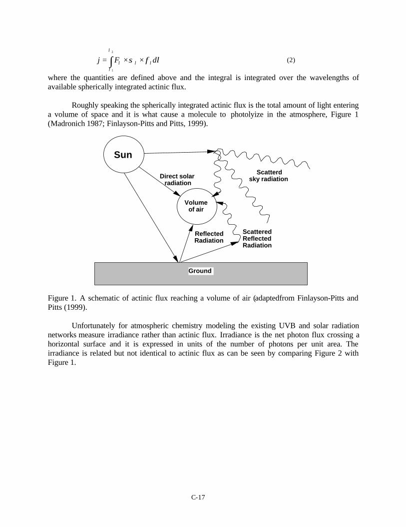
C-17
j = Fλλ1
λ 2
∫ ×σλ × φλdλ (2)
where the quantities are defined above and the integral is integrated over the wavelengths ofavailable spherically integrated actinic flux.
Roughly speaking the spherically integrated actinic flux is the total amount of light enteringa volume of space and it is what cause a molecule to photolyize in the atmosphere, Figure 1(Madronich 1987; Finlayson-Pitts and Pitts, 1999).
Sun
Direct solar radiation
Volume of air
Scatterd sky radiation
Ground
Reflected Radiation
Scattered Reflected Radiation
Figure 1. A schematic of actinic flux reaching a volume of air (adaptedfrom Finlayson-Pitts andPitts (1999).
Unfortunately for atmospheric chemistry modeling the existing UVB and solar radiationnetworks measure irradiance rather than actinic flux. Irradiance is the net photon flux crossing ahorizontal surface and it is expressed in units of the number of photons per unit area. Theirradiance is related but not identical to actinic flux as can be seen by comparing Figure 2 withFigure 1.
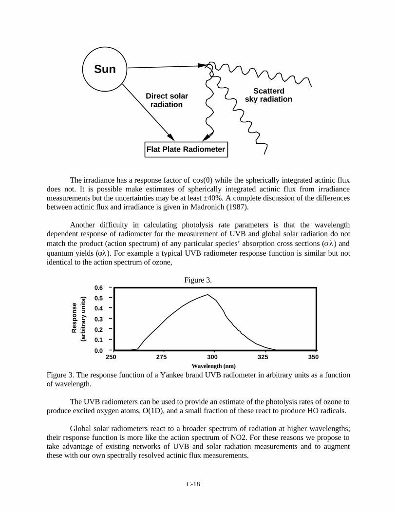
C-18
Sun
Direct solar radiation
Scatterd sky radiation
Flat Plate Radiometer
The irradiance has a response factor of cos(θ) while the spherically integrated actinic fluxdoes not. It is possible make estimates of spherically integrated actinic flux from irradiancemeasurements but the uncertainties may be at least ±40%. A complete discussion of the differencesbetween actinic flux and irradiance is given in Madronich (1987).
Another difficulty in calculating photolysis rate parameters is that the wavelengthdependent response of radiometer for the measurement of UVB and global solar radiation do notmatch the product (action spectrum) of any particular species’ absorption cross sections (σλ) andquantum yields (φλ). For example a typical UVB radiometer response function is similar but notidentical to the action spectrum of ozone,
Figure 3.
Res
po
nse
(a
rbitr
ary
un
its)
0.0
0.1
0.2
0.3
0.4
0.5
0.6
250 275 300 325 350Wavelength (nm)
Figure 3. The response function of a Yankee brand UVB radiometer in arbitrary units as a functionof wavelength.
The UVB radiometers can be used to provide an estimate of the photolysis rates of ozone toproduce excited oxygen atoms, O(1D), and a small fraction of these react to produce HO radicals.
Global solar radiometers react to a broader spectrum of radiation at higher wavelengths;their response function is more like the action spectrum of NO2. For these reasons we propose totake advantage of existing networks of UVB and solar radiation measurements and to augmentthese with our own spectrally resolved actinic flux measurements.
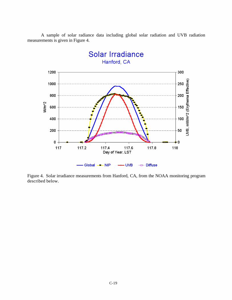
C-19
A sample of solar radiance data including global solar radiation and UVB radiationmeasurements is given in Figure 4.
Figure 4. Solar irradiance measurements from Hanford, CA, from the NOAA monitoring programdescribed below.
Appendix D-1
Supplemental Air Quality Site Descriptions and Installation Information
Site Information
TABLE OF CONTENTS
S0 Sites
Bella Vista ......................................................................................................................................................... D-1Lambie Road...................................................................................................................................................... D-2Sloughhouse ...................................................................................................................................................... D-4San Martin.......................................................................................................................................................... D-6Kettleman City .................................................................................................................................................. D-8McKittrick ....................................................................................................................................................... D-10Red Hills (SLOAPCD) ................................................................................................................................... D-12
S1 Sites
Sutter Butte ...................................................................................................................................................... D-14White Cloud..................................................................................................................................................... D-16Bodega Bay...................................................................................................................................................... D-18San Leandro..................................................................................................................................................... D-20San Jose 4th Street .......................................................................................................................................... D-21Bruceville......................................................................................................................................................... D-23San Andreas..................................................................................................................................................... D-25Turlock............................................................................................................................................................. D-27Piedras Blancas (South Central Coast) .......................................................................................................... D-29Angiola............................................................................................................................................................. D-31
S2 SitesBethel Island .................................................................................................................................................... D-33Patterson Pass.................................................................................................................................................. D-35Pacheco Pass.................................................................................................................................................... D-37Trimmer ........................................................................................................................................................... D-39Arvin................................................................................................................................................................. D-41
Research SitesSunol ................................................................................................................................................................ D-43Granite Bay...................................................................................................................................................... D-45Parlier ............................................................................................................................................................... D-47
Other SitesShasta Lake...................................................................................................................................................... D-49Camp Roberts.................................................................................................................................................. D-50
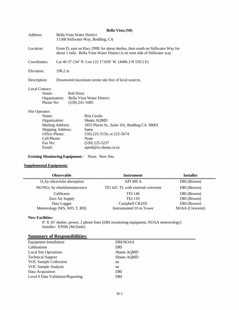
D-1
Bella Vista (S0)Address: Bella Vista Water District
11368 Stillwater Way, Redding, CA
Location: From I5, east on Hwy 299E for about 4miles, then south on Stillwater Way for about 1 mile. Bella Vista Water District is on west side of Stillwater way.
Coordinates: Lat 40 37.134’ N Lon 122 17.839’ W (4496.3 N 559.5 E)
Elevation: 198.2 m
Description: Downwind maximum ozone site free of local sources.
Local Contact:Name: Bob DietzOrganization: Bella Vista Water DistrictPhone No: (530) 241-1085
Site Operator:Name: Rita CirulisOrganization: Shasta AQMDMailing Address: 1855 Placer St., Suite 101, Redding CA 96001Shipping Address: SameOffice Phone: 530) 225-5156, or 225-5674Cell Phone: NoneFax No: (530) 225-5237Email: [email protected]
Existing Monitoring Equipment : None. New Site.
Supplemental Equipment:
Observable Instrument Installer
O3 by ultraviolet absorption API 400 A DRI (Bowen)
NO/NOY by chemiluminescence TEI 42C TL with external converter DRI (Bowen)
Calibrator TEI 146 DRI (Bowen)Zero Air Supply TEI 110 DRI (Bowen)
Data Logger Campbell CR10X DRI (Bowen)Meteorology (WS, WD, T, RH) Instrumented 10 m Tower NOAA (Crescenti)
New Facilities:8’ X 10’ shelter, power, 2 phone lines (DRI monitoring equipment, NOAA meteorology)Installer: ENSR (McDade)
Summary of Responsibilities:Equipment Installation DRI/NOAACalibrations DRILocal Site Operations Shasta AQMDTechnical Support Shasta AQMDVOC Sample Collection naVOC Sample Analysis naData Acquisition DRILevel 0 Data Validation/Reporting DRI
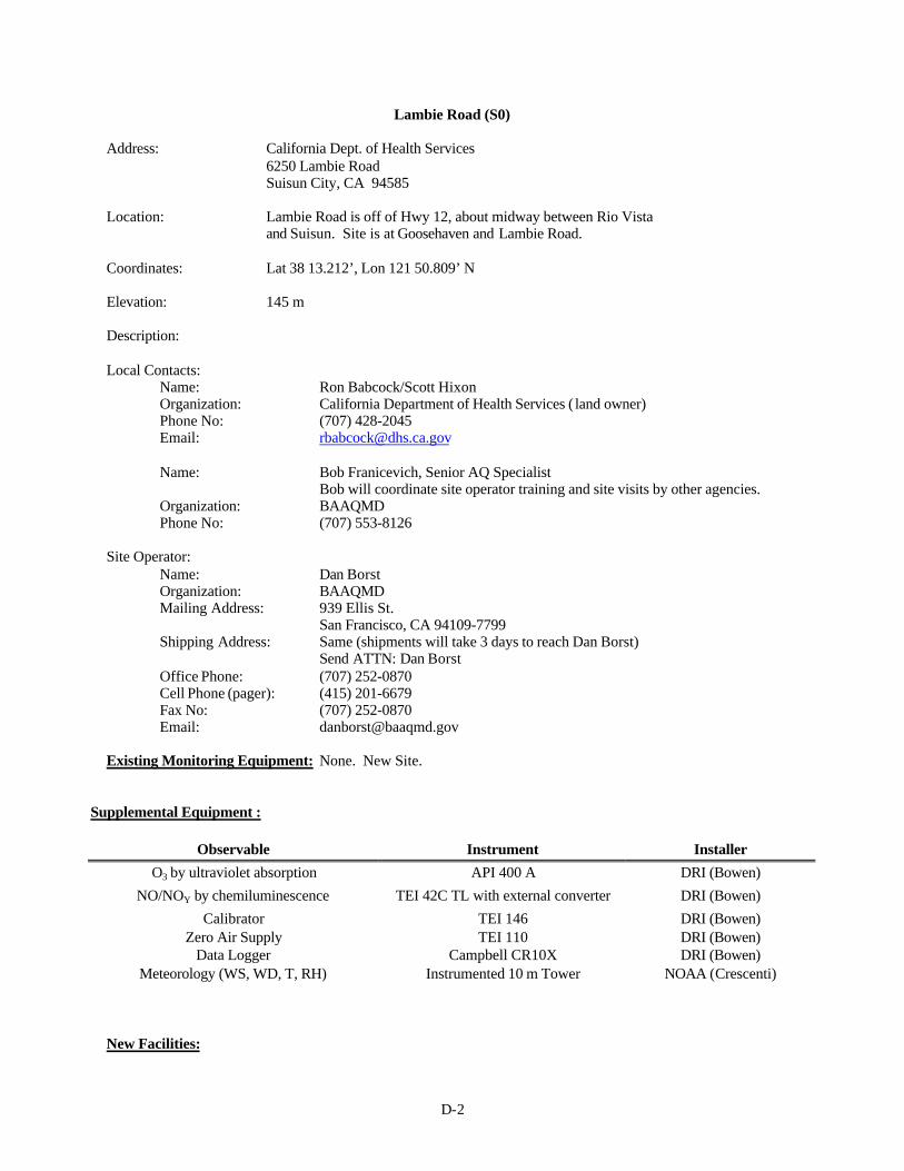
D-2
Lambie Road (S0)
Address: California Dept. of Health Services6250 Lambie RoadSuisun City, CA 94585
Location: Lambie Road is off of Hwy 12, about midway between Rio Vistaand Suisun. Site is at Goosehaven and Lambie Road.
Coordinates: Lat 38 13.212’, Lon 121 50.809’ N
Elevation: 145 m
Description:
Local Contacts:Name: Ron Babcock/Scott HixonOrganization: California Department of Health Services ( land owner)Phone No: (707) 428-2045Email: [email protected]
Name: Bob Franicevich, Senior AQ SpecialistBob will coordinate site operator training and site visits by other agencies.
Organization: BAAQMDPhone No: (707) 553-8126
Site Operator:Name: Dan BorstOrganization: BAAQMDMailing Address: 939 Ellis St.
San Francisco, CA 94109-7799Shipping Address: Same (shipments will take 3 days to reach Dan Borst)
Send ATTN: Dan BorstOffice Phone: (707) 252-0870Cell Phone (pager): (415) 201-6679Fax No: (707) 252-0870Email: [email protected]
Existing Monitoring Equipment: None. New Site.
Supplemental Equipment :
Observable Instrument Installer
O3 by ultraviolet absorption API 400 A DRI (Bowen)
NO/NOY by chemiluminescence TEI 42C TL with external converter DRI (Bowen)
Calibrator TEI 146 DRI (Bowen)Zero Air Supply TEI 110 DRI (Bowen)
Data Logger Campbell CR10X DRI (Bowen)Meteorology (WS, WD, T, RH) Instrumented 10 m Tower NOAA (Crescenti)
New Facilities:
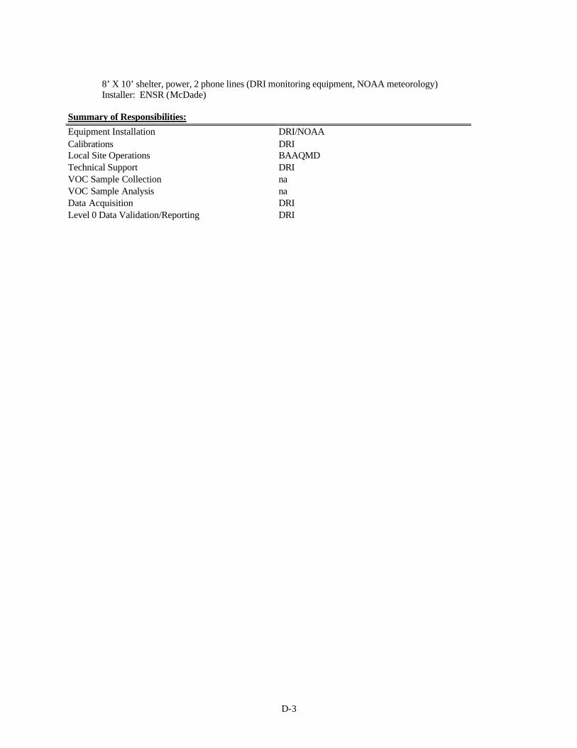
D-3
8’ X 10’ shelter, power, 2 phone lines (DRI monitoring equipment, NOAA meteorology)Installer: ENSR (McDade)
Summary of Responsibilities:
Equipment Installation DRI/NOAACalibrations DRILocal Site Operations BAAQMDTechnical Support DRIVOC Sample Collection naVOC Sample Analysis naData Acquisition DRILevel 0 Data Validation/Reporting DRI
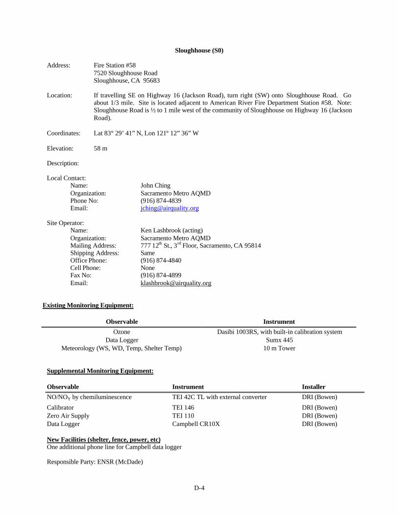
D-4
Sloughhouse (S0)
Address: Fire Station #587520 Sloughhouse RoadSloughhouse, CA 95683
Location: If travelling SE on Highway 16 (Jackson Road), turn right (SW) onto Sloughhouse Road. Goabout 1/3 mile. Site is located adjacent to American River Fire Department Station #58. Note:Sloughhouse Road is ½ to 1 mile west of the community of Sloughhouse on Highway 16 (JacksonRoad).
Coordinates: Lat 83° 29’ 41” N, Lon 121° 12” 36” W
Elevation: 58 m
Description:
Local Contact:Name: John Ching Organization: Sacramento Metro AQMDPhone No: (916) 874-4839Email: [email protected]
Site Operator:Name: Ken Lashbrook (acting)Organization: Sacramento Metro AQMDMailing Address: 777 12th St., 3rd Floor, Sacramento, CA 95814Shipping Address: SameOffice Phone: (916) 874-4840Cell Phone: NoneFax No: (916) 874-4899Email: [email protected]
Existing Monitoring Equipment:
Observable Instrument
Ozone Dasibi 1003RS, with built-in calibration systemData Logger Sumx 445
Meteorology (WS, WD, Temp, Shelter Temp) 10 m Tower
Supplemental Monitoring Equipment:
Observable Instrument Installer
NO/NOY by chemiluminescence TEI 42C TL with external converter DRI (Bowen)
Calibrator TEI 146 DRI (Bowen)Zero Air Supply TEI 110 DRI (Bowen)Data Logger Campbell CR10X DRI (Bowen)
New Facilities (shelter, fence, power, etc)One additional phone line for Campbell data logger
Responsible Party: ENSR (McDade)
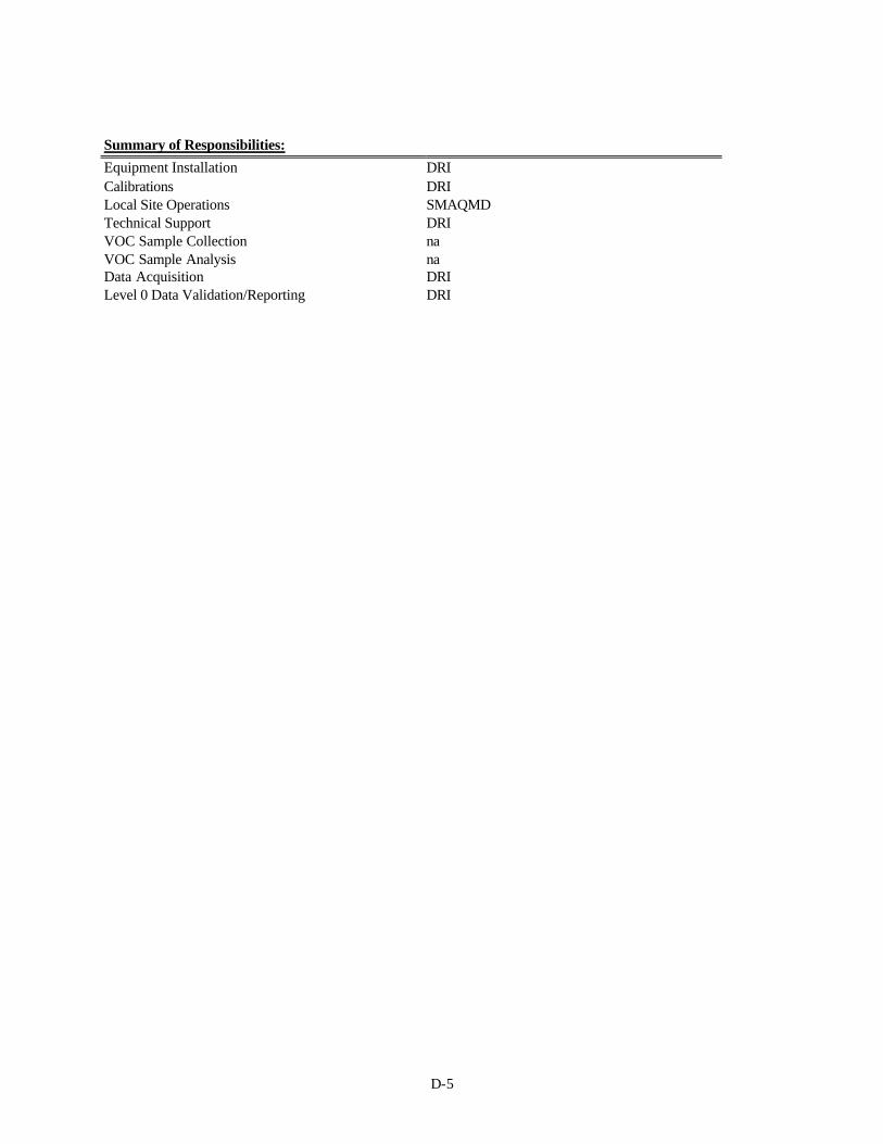
D-5
Summary of Responsibilities:
Equipment Installation DRICalibrations DRILocal Site Operations SMAQMDTechnical Support DRIVOC Sample Collection naVOC Sample Analysis naData Acquisition DRILevel 0 Data Validation/Reporting DRI
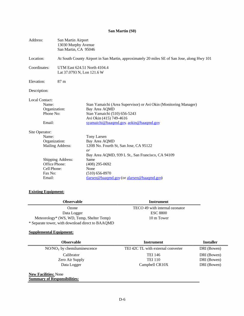
D-6
San Martin (S0)
Address: San Martin Airport13030 Murphy AvenueSan Martin, CA 95046
Location: At South County Airport in San Martin, approximately 20 miles SE of San Jose, along Hwy 101
Coordinates: UTM East 624.51 North 4104.4Lat 37.0793 N, Lon 121.6 W
Elevation: 87 m
Description:
Local Contact:Name: Stan Yamaichi (Area Supervisor) or Avi Okin (Monitoring Manager)Organization: Bay Area AQMDPhone No: Stan Yamaichi (510) 656-5243
Avi Okin (415) 749-4616Email: [email protected], [email protected]
Site Operator:Name: Tony Larsen Organization: Bay Area AQMDMailing Address: 120B No. Fourth St, San Jose, CA 95122
orBay Area AQMD, 939 L St., San Francisco, CA 94109
Shipping Address: SameOffice Phone: (408) 295-0692Cell Phone: NoneFax No: (510) 656-8970Email: [email protected] (or [email protected])
Existing Equipment:
Observable Instrument
Ozone TECO 49 with internal ozonatorData Logger ESC 8800
Meteorology* (WS, WD, Temp, Shelter Temp) 10 m Tower* Separate tower, with download direct to BAAQMD
Supplemental Equipment:
Observable Instrument Installer
NO/NOY by chemiluminescence TEI 42C TL with external converter DRI (Bowen)
Calibrator TEI 146 DRI (Bowen)Zero Air Supply TEI 110 DRI (Bowen)
Data Logger Campbell CR10X DRI (Bowen)
New Facilities: NoneSummary of Responsibilities:

D-7
Equipment Installation DRICalibrations DRILocal Site Operations BAAQMDTechnical Support BAAQMDVOC Sample Collection naVOC Sample Analysis naData Acquisition DRILevel 0 Data Validation/Reporting DRI
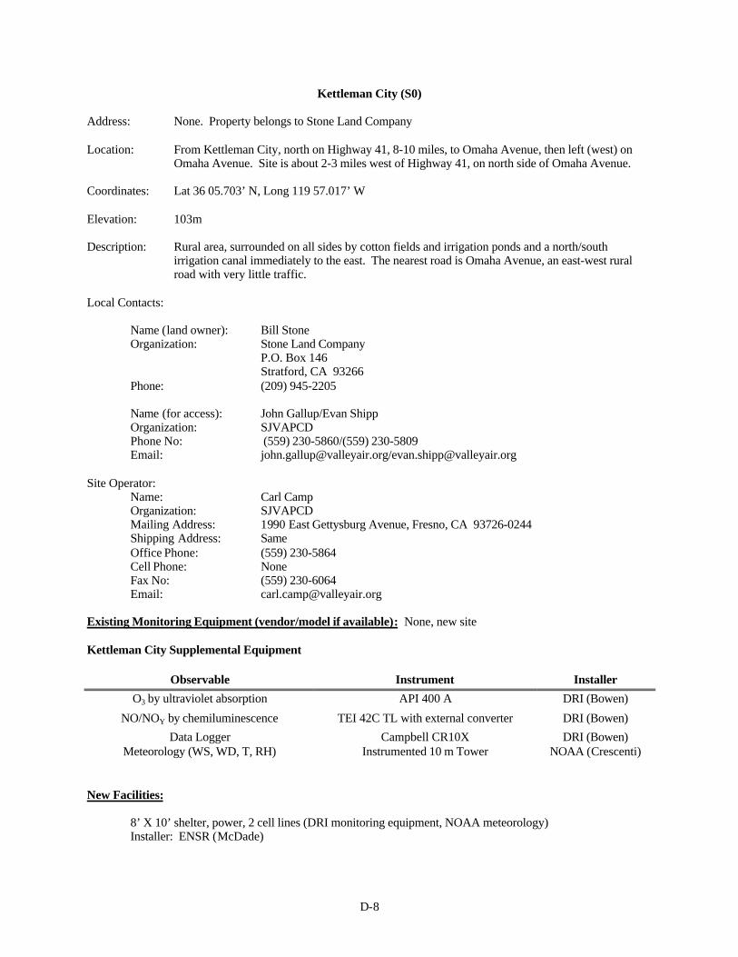
D-8
Kettleman City (S0)
Address: None. Property belongs to Stone Land Company
Location: From Kettleman City, north on Highway 41, 8-10 miles, to Omaha Avenue, then left (west) onOmaha Avenue. Site is about 2-3 miles west of Highway 41, on north side of Omaha Avenue.
Coordinates: Lat 36 05.703’ N, Long 119 57.017’ W
Elevation: 103m
Description: Rural area, surrounded on all sides by cotton fields and irrigation ponds and a north/southirrigation canal immediately to the east. The nearest road is Omaha Avenue, an east-west ruralroad with very little traffic.
Local Contacts:
Name (land owner): Bill StoneOrganization: Stone Land Company
P.O. Box 146Stratford, CA 93266
Phone: (209) 945-2205
Name (for access): John Gallup/Evan ShippOrganization: SJVAPCDPhone No: (559) 230-5860/(559) 230-5809Email: [email protected]/[email protected]
Site Operator:Name: Carl CampOrganization: SJVAPCD Mailing Address: 1990 East Gettysburg Avenue, Fresno, CA 93726-0244Shipping Address: SameOffice Phone: (559) 230-5864Cell Phone: NoneFax No: (559) 230-6064Email: [email protected]
Existing Monitoring Equipment (vendor/model if available): None, new site
Kettleman City Supplemental Equipment
Observable Instrument Installer
O3 by ultraviolet absorption API 400 A DRI (Bowen)
NO/NOY by chemiluminescence TEI 42C TL with external converter DRI (Bowen)
Data Logger Campbell CR10X DRI (Bowen)Meteorology (WS, WD, T, RH) Instrumented 10 m Tower NOAA (Crescenti)
New Facilities:
8’ X 10’ shelter, power, 2 cell lines (DRI monitoring equipment, NOAA meteorology)Installer: ENSR (McDade)

D-9
Summary of Responsibilities:
Equipment Installation DRI/NOAACalibrations DRILocal Site Operations SJVUAPCDTechnical Support DRIVOC Sample Collection naVOC Sample Analysis naData Acquisition DRILevel 0 Data Validation/Reporting DRI
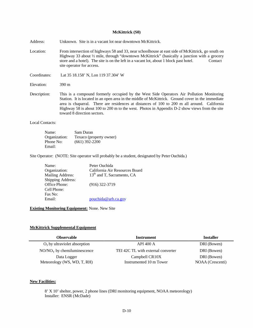
D-10
McKittrick (S0)
Address: Unknown. Site is in a vacant lot near downtown McKittrick.
Location: From intersection of highways 58 and 33, near schoolhouse at east side of McKittrick, go south onHighway 33 about ½ mile, through “downtown McKittrick” (basically a junction with a grocerystore and a hotel). The site is on the left in a vacant lot, about 1 block past hotel. Contactsite operator for access.
Coordinates: Lat 35 18.158’ N, Lon 119 37.304’ W
Elevation: 390 m
Description: This is a compound formerly occupied by the West Side Operators Air Pollution MonitoringStation. It is located in an open area in the middle of McKittrick. Ground cover in the immediatearea is chaparral. There are residences at distances of 100 to 200 m all around. CaliforniaHighway 58 is about 100 to 200 m to the west. Photos in Appendix D-2 show views from the sitetoward 8 direction sectors.
Local Contacts:
Name: Sam DuranOrganization: Texaco (property owner)Phone No: (661) 392-2200Email:
Site Operator: (NOTE: Site operator will probably be a student, designated by Peter Ouchida.)
Name: Peter OuchidaOrganization: California Air Resources BoardMailing Address: 13th and T, Sacramento, CAShipping Address: Office Phone: (916) 322-3719Cell Phone: Fax No: Email: [email protected]
Existing Monitoring Equipment: None. New Site
McKittrick Supplemental Equipment
Observable Instrument Installer
O3 by ultraviolet absorption API 400 A DRI (Bowen)
NO/NOY by chemiluminescence TEI 42C TL with external converter DRI (Bowen)
Data Logger Campbell CR10X DRI (Bowen)Meteorology (WS, WD, T, RH) Instrumented 10 m Tower NOAA (Crescenti)
New Facilities:
8’ X 10’ shelter, power, 2 phone lines (DRI monitoring equipment, NOAA meteorology)Installer: ENSR (McDade)

D-11
Summary of Responsibilities:
Equipment Installation DRI (Bowen), NOAA(Crescenti)Calibrations DRI(Bowen)Local Site Operations ARB (Ouchida)Technical Support ARB (Ouchida)VOC Sample Collection naVOC Sample Analysis naData Acquisition DRILevel 0 Data Validation/Reporting DRI
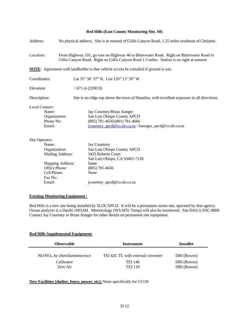
D-12
Red Hills (East County Monitoring Site, S0)
Address: No physical address. Site is at summit of Gillis Canyon Road, 1.25 miles southeast of Cholame.
Location: From Highway 101, go east on Highway 46 to Bitterwater Road. Right on Bitterwater Road toGillis Canyon Road. Right on Gillis Canyon Road 1.3 miles. Station is on right at summit
NOTE: Agreement with landholder is that vehicle access be curtailed if ground is wet.
Coordinates: Lat 35° 38’ 37” N, Lon 120° 13’ 50” W
Elevation: ~ 671 m (2200 ft)
Description: Site is on ridge top above the town of Shandon, with excellent exposure in all directions.
Local Contact:Name: Jay Courtney/Brian AungerOrganization: San Luis Obispo County APCDPhone No: (805) 781-4656/(801) 781-4666Email: [email protected] / [email protected]
Site Operator:Name: Jay CourtneyOrganization: San Luis Obispo County APCDMailing Address: 3433 Roberto Court
San Luis Obispo, CA 93401-7126Shipping Address: SameOffice Phone: (805) 781-4656Cell Phone: NoneFax No: Email: [email protected]
Existing Monitoring Equipment :
Red Hills is a new site being installed by SLOCAPCD. It will be a permanent ozone site, operated by that agency.Ozone analyzer is a Dasibi 1003AH. Meteorology (WS,WD, Temp) will also be monitored. Site DAS is ESC 8800.Contact Jay Courtney or Brian Aunger for other details on permanent site equipment.
Red Hills Supplemental Equipment:
Observable Instrument Installer
NO/NOY by chemiluminescence TEI 42C TL with external converter DRI (Bowen)
Calibrator TEI 146 DRI (Bowen)Zero Air TEI 110 DRI (Bowen)
New Facilities (shelter, fence, power, etc): None specifically for CCOS
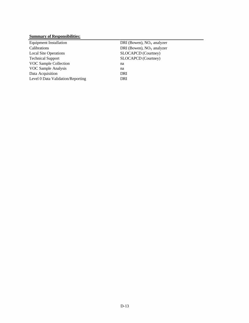
D-13
Summary of Responsibilities:
Equipment Installation DRI (Bowen), NOY analyzerCalibrations DRI (Bowen), NOY analyzerLocal Site Operations SLOCAPCD (Courtney)Technical Support SLOCAPCD (Courtney)VOC Sample Collection naVOC Sample Analysis naData Acquisition DRILevel 0 Data Validation/Reporting DRI
D-14
Sutter Butte (S1)
Address: South Butte, Building A
Location: From Highway 20, go north on Acacia Avenue. (There is a Minimart at the junction.) Go north onAcacia, through Sutter. Acacia turns into South Butte Road. Take sharp left turn at what lookslike a storage yard. Go to white gate, 2-3 miles, on right (north) side.
NOTE: Access is very restricted. Property belongs to American Towers. Contacts at AmericanTowers are Jim Pederson (cell phone (916) 768-8039), Jake Kley – Maintenance Supervisor ((530)458-2118), or possibly Gabrielle Turner-Ayres – Access Coordinator ((510) 236-3803 ext 279).Refer to Rick Rigsby, ARB site operator. (Or contact Rick Rigsby first).
Coordinates: Lat 39° 9’ 20” N, Lon 121° 43’00” W
Elevation: 659 m (2160 ft)
Description: Top of Butte
Local Contacts:
Name: Jim Pederson/Jake KleyOrganization: American TowersPhone No: (916) 768-8039/(530) 458-2118Email:
Name: Larry MolekOrganization: ARBPhone No: 916) 327-4889Email: [email protected]
Site Operator (for CCOS Operations):
Name: John BowenOrganization: Desert Research InstituteMailing Address: 2215 Raggio Parkway
Reno, NV 89512Shipping Address: SameOffice Phone: (775) 674-7044Cell Phone: (775) 560-9246Fax No: (775) 674-7009Email: [email protected]
Site Operator (for routine (Non-CCOS) operations):
Name: Rick RigsbyOrganization: ARBMailing Address: State of California Air Resources Board
773 Almond St.Yuba City, CA 95991
Shipping Address: SameOffice Phone: (530) 671-7615Cell Phone: (530) 755-9116Fax No: noneEmail: [email protected]
Sutter Buttes Existing Equipment:
D-15
Observable Instrument
Ozone API 400 with Internal Zero/SpanData Logger ESC 8800Meteorology (NOT ARB's, belongs toNowCasting
Sutter Buttes Supplemental Equipment:
Observable Instrument Installer
NOY/NOY by chemiluminescence TEI 42C TL with external converter DRI (Bowen)
C2 - C12 HC from canisters DRI Multi-Channel Sequential HC Sampler DRI (Zielinska)
C1 - C7 carbonyls from DNPH AtmAA Carbonyl Sampler AtmAA (Fung)
Outside Shelter for DRI HC sampler DRI HC Sampler Shelter DRI (Zielinska)
New Facilities: None
Summary of Responsibilities
Equipment Installation DRI/AtmAA(Carbonyls)Calibrations DRILocal Site Operations DRITechnical Support DRIVOC Sample Collection DRI (canisters)/AtmAA (Carbonyls)VOC Sample Analysis DRI (canisters)/AtmAA (Carbonyls)Data Acquisition DRILevel 0 Data Validation/Reporting DRI
D-16
White Cloud (S1)
Address: 26533 State Highway 20Nevada City, CA
Location: From I80, take Nevada City exit (Highway 20). Site is on Highway 20 at the WhiteCloud Forest Service station, 12-15 miles east of Nevada City, on south side of highway.It is across from the White Cloud rest stop, on north side of highway. Gate is normallyopen.
Coordinates: Lat 39.3166 N, Lon 120.8444 W
Elevation: 1302 m
Description:
Local Contact:
Name: Larry MolekOrganization: ARBPhone No: (916) 327-4889Email: [email protected]
Site Operator (for CCOS Operations):
Name: John BowenOrganization: Desert Research InstituteMailing Address: 2215 Raggio Parkway
Reno, NV 89512Shipping Address: SameOffice Phone: (775) 674-7044Cell Phone: (775) 560-9246Fax No: (775) 674-7009Email: [email protected]
Site Operator (for routine (non-CCOS) operations):
Name: Kent Breitwieser Organization: ARBMailing Address: Shipping Address: Office Phone: (916) 784-8065Cell Phone: Fax No: Email: [email protected]
White Cloud Existing Equipment:
Observable Instrument
Ozone API 400 with Internal Zero/SpanData Logger ESC 8800Meteorology
D-17
White Cloud Supplemental Equipment:
Observable Instrument Installer
NOY/NOY by chemiluminescence TEI 42C TL with external converter DRI (Bowen)
C2 - C12 HC from canisters DRI Multi-Channel Sequential HC Sampler DRI (Zielinska)
C1 - C7 carbonyls from DNPH AtmAA Carbonyl Sampler AtmAA (Fung)
Outside Shelter for DRI HC sampler DRI HC Sampler Shelter DRI (Zielinska)
New Facilities: None
Summary of Responsibilities
Equipment Installation DRI/AtmAA(Carbonyls)Calibrations DRILocal Site Operations DRITechnical Support DRIVOC Sample Collection DRI (canisters)/AtmAA (Carbonyls)VOC Sample Analysis DRI (canisters)/AtmAA (Carbonyls)Data Acquisition DRILevel 0 Data Validation/Reporting DRI
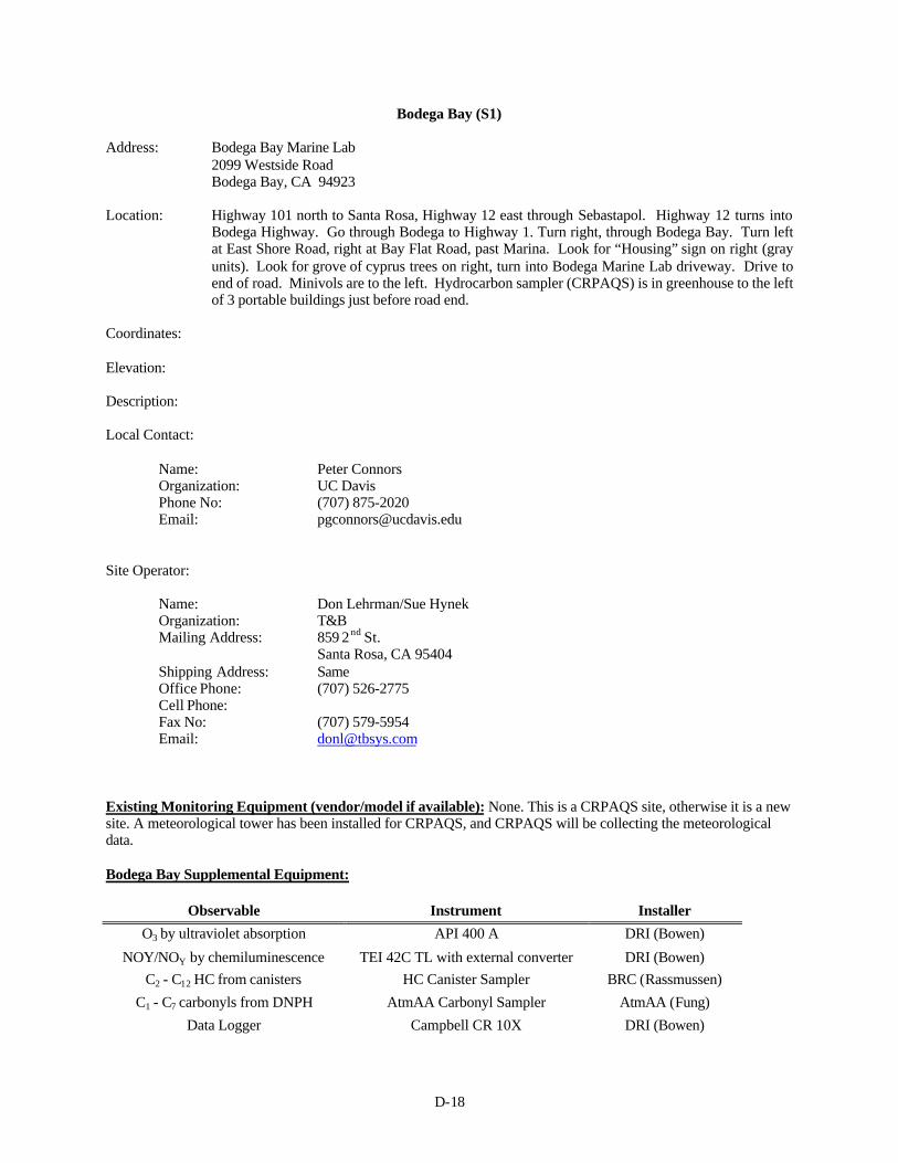
D-18
Bodega Bay (S1)
Address: Bodega Bay Marine Lab2099 Westside RoadBodega Bay, CA 94923
Location: Highway 101 north to Santa Rosa, Highway 12 east through Sebastapol. Highway 12 turns intoBodega Highway. Go through Bodega to Highway 1. Turn right, through Bodega Bay. Turn leftat East Shore Road, right at Bay Flat Road, past Marina. Look for “Housing” sign on right (grayunits). Look for grove of cyprus trees on right, turn into Bodega Marine Lab driveway. Drive toend of road. Minivols are to the left. Hydrocarbon sampler (CRPAQS) is in greenhouse to the leftof 3 portable buildings just before road end.
Coordinates:
Elevation:
Description:
Local Contact:
Name: Peter ConnorsOrganization: UC DavisPhone No: (707) 875-2020Email: [email protected]
Site Operator:
Name: Don Lehrman/Sue HynekOrganization: T&BMailing Address: 859 2 nd St.
Santa Rosa, CA 95404Shipping Address: SameOffice Phone: (707) 526-2775Cell Phone: Fax No: (707) 579-5954Email: [email protected]
Existing Monitoring Equipment (vendor/model if available): None. This is a CRPAQS site, otherwise it is a newsite. A meteorological tower has been installed for CRPAQS, and CRPAQS will be collecting the meteorologicaldata.
Bodega Bay Supplemental Equipment:
Observable Instrument Installer
O3 by ultraviolet absorption API 400 A DRI (Bowen)
NOY/NOY by chemiluminescence TEI 42C TL with external converter DRI (Bowen)
C2 - C12 HC from canisters HC Canister Sampler BRC (Rassmussen)
C1 - C7 carbonyls from DNPH AtmAA Carbonyl Sampler AtmAA (Fung)
Data Logger Campbell CR 10X DRI (Bowen)
D-19
New Facilities:
8’ X 10’ shelter (in addition to the CRPAQS shelter), power, 1 phone line (DRI monitoring equipment)Installer: ENSR (McDade)
Summary of Responsibilities:
Equipment Installation DRI/AtmAA(Carbonyls)/BRC(HC Canisters)Calibrations DRI (Bowen)Local Site Operations T&B(Lehrman)Technical SupportVOC Sample Collection T&BVOC Sample Analysis BRC(HC canisters)/AtmAA(Carbonyls)Data Acquisition DRI(Bowen)Level 0 Data Validation/Reporting DRI(Bowen)
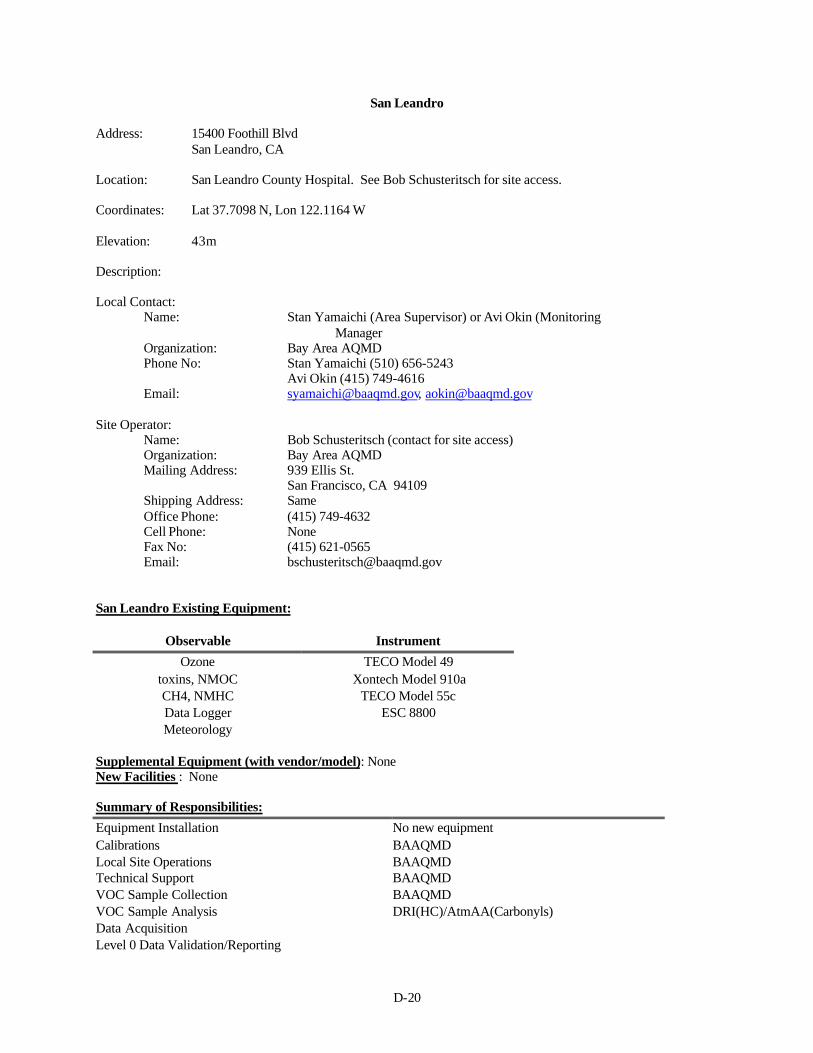
D-20
San Leandro
Address: 15400 Foothill BlvdSan Leandro, CA
Location: San Leandro County Hospital. See Bob Schusteritsch for site access.
Coordinates: Lat 37.7098 N, Lon 122.1164 W
Elevation: 43m
Description:
Local Contact:Name: Stan Yamaichi (Area Supervisor) or Avi Okin (Monitoring
ManagerOrganization: Bay Area AQMDPhone No: Stan Yamaichi (510) 656-5243
Avi Okin (415) 749-4616Email: [email protected], [email protected]
Site Operator:Name: Bob Schusteritsch (contact for site access) Organization: Bay Area AQMDMailing Address: 939 Ellis St.
San Francisco, CA 94109Shipping Address: SameOffice Phone: (415) 749-4632Cell Phone: NoneFax No: (415) 621-0565Email: [email protected]
San Leandro Existing Equipment:
Observable Instrument
Ozone TECO Model 49toxins, NMOC Xontech Model 910aCH4, NMHC TECO Model 55cData Logger ESC 8800Meteorology
Supplemental Equipment (with vendor/model): NoneNew Facilities : None
Summary of Responsibilities:
Equipment Installation No new equipmentCalibrations BAAQMDLocal Site Operations BAAQMDTechnical Support BAAQMDVOC Sample Collection BAAQMDVOC Sample Analysis DRI(HC)/AtmAA(Carbonyls)Data AcquisitionLevel 0 Data Validation/Reporting
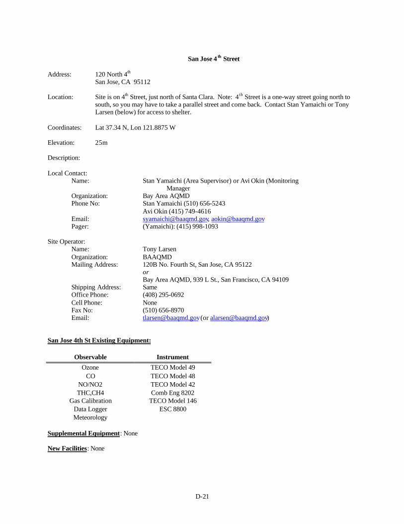
D-21
San Jose 4 th Street
Address: 120 North 4th
San Jose, CA 95112
Location: Site is on 4th Street, just north of Santa Clara. Note: 4th Street is a one-way street going north tosouth, so you may have to take a parallel street and come back. Contact Stan Yamaichi or TonyLarsen (below) for access to shelter.
Coordinates: Lat 37.34 N, Lon 121.8875 W
Elevation: 25m
Description:
Local Contact:Name: Stan Yamaichi (Area Supervisor) or Avi Okin (Monitoring
ManagerOrganization: Bay Area AQMDPhone No: Stan Yamaichi (510) 656-5243
Avi Okin (415) 749-4616Email: [email protected], [email protected]: (Yamaichi): (415) 998-1093
Site Operator:Name: Tony Larsen Organization: BAAQMDMailing Address: 120B No. Fourth St, San Jose, CA 95122
orBay Area AQMD, 939 L St., San Francisco, CA 94109
Shipping Address: SameOffice Phone: (408) 295-0692Cell Phone: NoneFax No: (510) 656-8970Email: [email protected] (or [email protected])
San Jose 4th St Existing Equipment:
Observable Instrument
Ozone TECO Model 49CO TECO Model 48
NO/NO2 TECO Model 42THC,CH4 Comb Eng 8202
Gas Calibration TECO Model 146Data Logger ESC 8800Meteorology
Supplemental Equipment: None
New Facilities: None
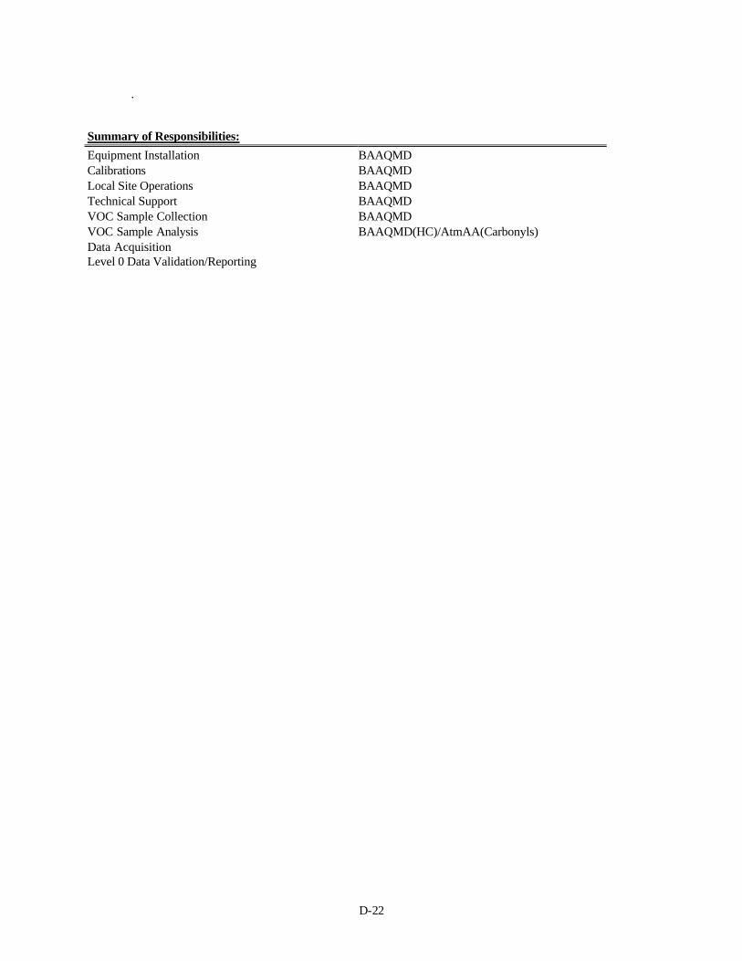
D-22
.
Summary of Responsibilities:
Equipment Installation BAAQMDCalibrations BAAQMDLocal Site Operations BAAQMDTechnical Support BAAQMDVOC Sample Collection BAAQMDVOC Sample Analysis BAAQMD(HC)/AtmAA(Carbonyls)Data AcquisitionLevel 0 Data Validation/Reporting
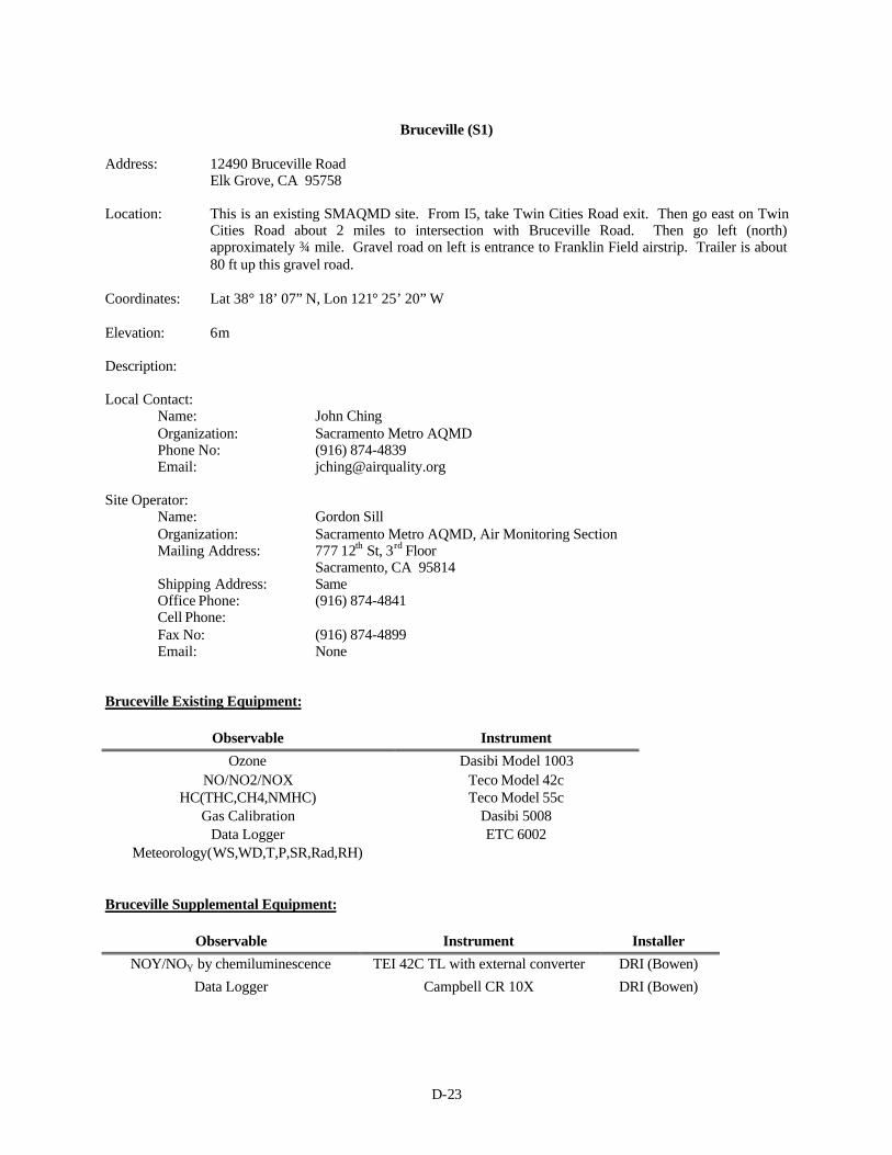
D-23
Bruceville (S1)
Address: 12490 Bruceville RoadElk Grove, CA 95758
Location: This is an existing SMAQMD site. From I5, take Twin Cities Road exit. Then go east on TwinCities Road about 2 miles to intersection with Bruceville Road. Then go left (north)approximately ¾ mile. Gravel road on left is entrance to Franklin Field airstrip. Trailer is about80 ft up this gravel road.
Coordinates: Lat 38° 18’ 07” N, Lon 121° 25’ 20” W
Elevation: 6m
Description:
Local Contact: Name: John ChingOrganization: Sacramento Metro AQMDPhone No: (916) 874-4839Email: [email protected]
Site Operator:Name: Gordon Sill Organization: Sacramento Metro AQMD, Air Monitoring SectionMailing Address: 777 12th St, 3rd Floor
Sacramento, CA 95814Shipping Address: SameOffice Phone: (916) 874-4841Cell Phone: Fax No: (916) 874-4899Email: None
Bruceville Existing Equipment:
Observable Instrument
Ozone Dasibi Model 1003NO/NO2/NOX Teco Model 42c
HC(THC,CH4,NMHC) Teco Model 55cGas Calibration Dasibi 5008
Data Logger ETC 6002Meteorology(WS,WD,T,P,SR,Rad,RH)
Bruceville Supplemental Equipment:
Observable Instrument Installer
NOY/NOY by chemiluminescence TEI 42C TL with external converter DRI (Bowen)
Data Logger Campbell CR 10X DRI (Bowen)
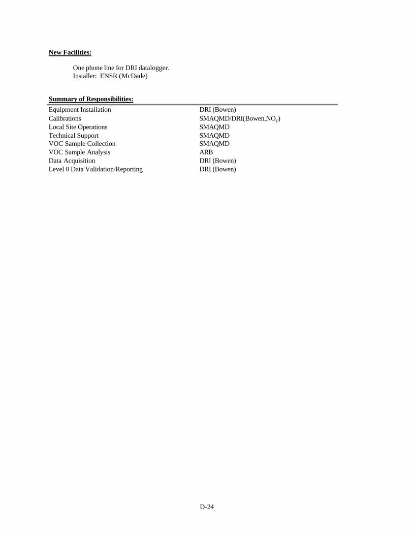
D-24
New Facilities:
One phone line for DRI datalogger.Installer: ENSR (McDade)
Summary of Responsibilities:
Equipment Installation DRI (Bowen)Calibrations SMAQMD/DRI(Bowen,NOy)Local Site Operations SMAQMDTechnical Support SMAQMDVOC Sample Collection SMAQMDVOC Sample Analysis ARBData Acquisition DRI (Bowen)Level 0 Data Validation/Reporting DRI (Bowen)
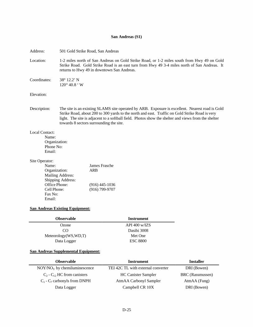
D-25
San Andreas (S1)
Address: 501 Gold Strike Road, San Andreas
Location: 1-2 miles north of San Andreas on Gold Strike Road, or 1-2 miles south from Hwy 49 on GoldStrike Road. Gold Strike Road is an east turn from Hwy 49 3-4 miles north of San Andreas. Itreturns to Hwy 49 in downtown San Andreas.
Coordinates: 38° 12.2’ N120° 40.8 ‘ W
Elevation:
Description: The site is an existing SLAMS site operated by ARB. Exposure is excellent. Nearest road is GoldStrike Road, about 200 to 300 yards to the north and east. Traffic on Gold Strike Road is verylight. The site is adjacent to a softball field. Photos show the shelter and views from the sheltertowards 8 sectors surrounding the site.
Local Contact:Name: Organization: Phone No:Email:
Site Operator:Name: James FrascheOrganization: ARBMailing Address: Shipping Address: Office Phone: (916) 445-1036Cell Phone: (916) 799-9707Fax No: Email:
San Andreas Existing Equipment:
Observable Instrument
Ozone API 400 w/IZSCO Dasibi 3008
Meteorology(WS,WD,T) Met OneData Logger ESC 8800
San Andreas Supplemental Equipment:
Observable Instrument Installer
NOY/NOY by chemiluminescence TEI 42C TL with external converter DRI (Bowen)
C2 - C12 HC from canisters HC Canister Sampler BRC (Rassmussen)
C1 - C7 carbonyls from DNPH AtmAA Carbonyl Sampler AtmAA (Fung)
Data Logger Campbell CR 10X DRI (Bowen)
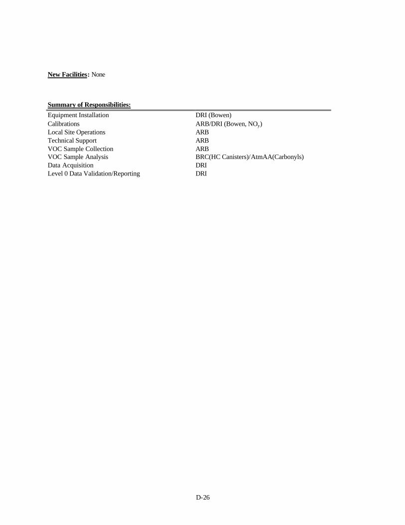
D-26
New Facilities: None
Summary of Responsibilities:
Equipment Installation DRI (Bowen)Calibrations ARB/DRI (Bowen, NOy)Local Site Operations ARBTechnical Support ARBVOC Sample Collection ARBVOC Sample Analysis BRC(HC Canisters)/AtmAA(Carbonyls)Data Acquisition DRILevel 0 Data Validation/Reporting DRI
D-27
Turlock (S1)
Address: 900 South Minaret Street, Turlock, CA
Location: Contact John Gallup or Warren LeLeaux (below) for access to site.
From Golden State Blvd, downtown Turlock, go east on East Avenue 2-3 blocks. Then go southon South Minaret, which angles to the southeast. Stay on Minaret to Cottonwood. Site is south ofthe intersection of South Minaret and Cottonwood..
Coordinates: 37° 29.298’ N Lon 120° 50.294’ W
Elevation: 56m
Description: The site is located south of the intersection of S. Minaret and Cottonwood, in a residential area.Photos in Appendix D-2 show the shelter and views from the shelter towards 8 sectorssurrounding the shelter. Streets in the immediate vicinity are very lightly traveled residentialstreets. The nearest major thoroughfare is Golden St. Blvd, 400 to 500 yards east of the site. ARailroad roughly parallels Golden St Blvd at this distance. Golden St Blvd is an elevated overpassat this distance, and can be seen in the “southwest” photo. The “View from Golden St. Blvd”photo was taken from this overpass looking back toward the shelter, which is roughly in the centerof the photo.
Local Contact:
Name: John Gallup (or Warren LeLeaux, below)Organization: San Joaquin Valley Unified APCDPhone No: (559) 230-5860Email:
Site Operator (for CCOS measurements):
Name: Don LehrmanOrganization: T&BMailing Address: 859 2 nd St.
Santa Rosa, CA 95404Shipping Address: SameOffice Phone: (707) 526-2775Cell Phone:Fax No: (707) 579-5954Email: [email protected]
Site Operator (for routine (non-CCOS) measurements):
Name: Warren LeLeauxOrganization: San Joaquin Valley Unified APCDMailing Address: ATTN: Warren LeLeaux
4230 Kiernan Avenue, Suite 130Modesto, CA 95356-9321
Shipping Address: Office Phone: (209) 557-6471Cell Phone (pager): (209) 569-6021 Fax No: (209) 557-6475Email: [email protected]
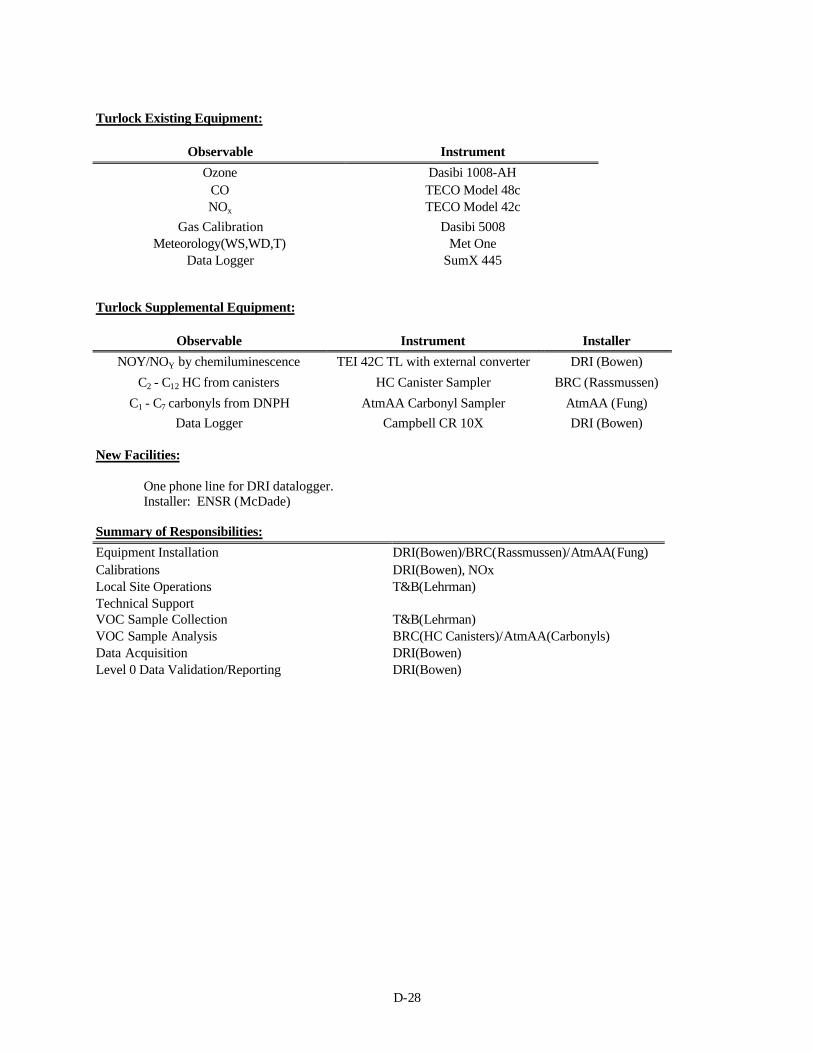
D-28
Turlock Existing Equipment:
Observable Instrument
Ozone Dasibi 1008-AHCO TECO Model 48cNOx TECO Model 42c
Gas Calibration Dasibi 5008Meteorology(WS,WD,T) Met One
Data Logger SumX 445
Turlock Supplemental Equipment:
Observable Instrument Installer
NOY/NOY by chemiluminescence TEI 42C TL with external converter DRI (Bowen)
C2 - C12 HC from canisters HC Canister Sampler BRC (Rassmussen)
C1 - C7 carbonyls from DNPH AtmAA Carbonyl Sampler AtmAA (Fung)
Data Logger Campbell CR 10X DRI (Bowen)
New Facilities:
One phone line for DRI datalogger.Installer: ENSR (McDade)
Summary of Responsibilities:
Equipment Installation DRI(Bowen)/BRC(Rassmussen)/AtmAA(Fung)Calibrations DRI(Bowen), NOxLocal Site Operations T&B(Lehrman)Technical SupportVOC Sample Collection T&B(Lehrman)VOC Sample Analysis BRC(HC Canisters)/AtmAA(Carbonyls)Data Acquisition DRI(Bowen)Level 0 Data Validation/Reporting DRI(Bowen)
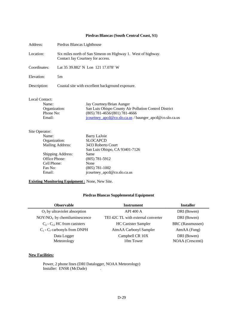
D-29
Piedras Blancas (South Central Coast, S1)
Address: Piedras Blancas Lighthouse
Location: Six miles north of San Simeon on Highway 1. West of highway.Contact Jay Courtney for access.
Coordinates: Lat 35 39.882’ N Lon 121 17.078’ W
Elevation: 5m
Description: Coastal site with excellent background exposure.
Local Contact:Name: Jay Courtney/Brian AungerOrganization: San Luis Obispo County Air Pollution Control DistrictPhone No: (805) 781-4656/(801) 781-4666Email: [email protected] / [email protected]
Site Operator:Name: Barry LaJoieOrganization: SLOCAPCDMailing Address: 3433 Roberto Court
San Luis Obispo, CA 93401-7126Shipping Address: SameOffice Phone: (805) 781-5912Cell Phone: NoneFax No: (805) 781-1002Email: [email protected]
Existing Monitoring Equipment : None, New Site.
Piedras Blancas Supplemental Equipment
Observable Instrument Installer
O3 by ultraviolet absorption API 400 A DRI (Bowen)
NOY/NOY by chemiluminescence TEI 42C TL with external converter DRI (Bowen)
C2 - C12 HC from canisters HC Canister Sampler BRC (Rassmussen)
C1 - C7 carbonyls from DNPH AtmAA Carbonyl Sampler AtmAA (Fung)
Data Logger Campbell CR 10X DRI (Bowen)Meteorology 10m Tower NOAA (Crescenti)
New Facilities:
Power, 2 phone lines (DRI Datalogger, NOAA Meteorology)Installer: ENSR (McDade) .
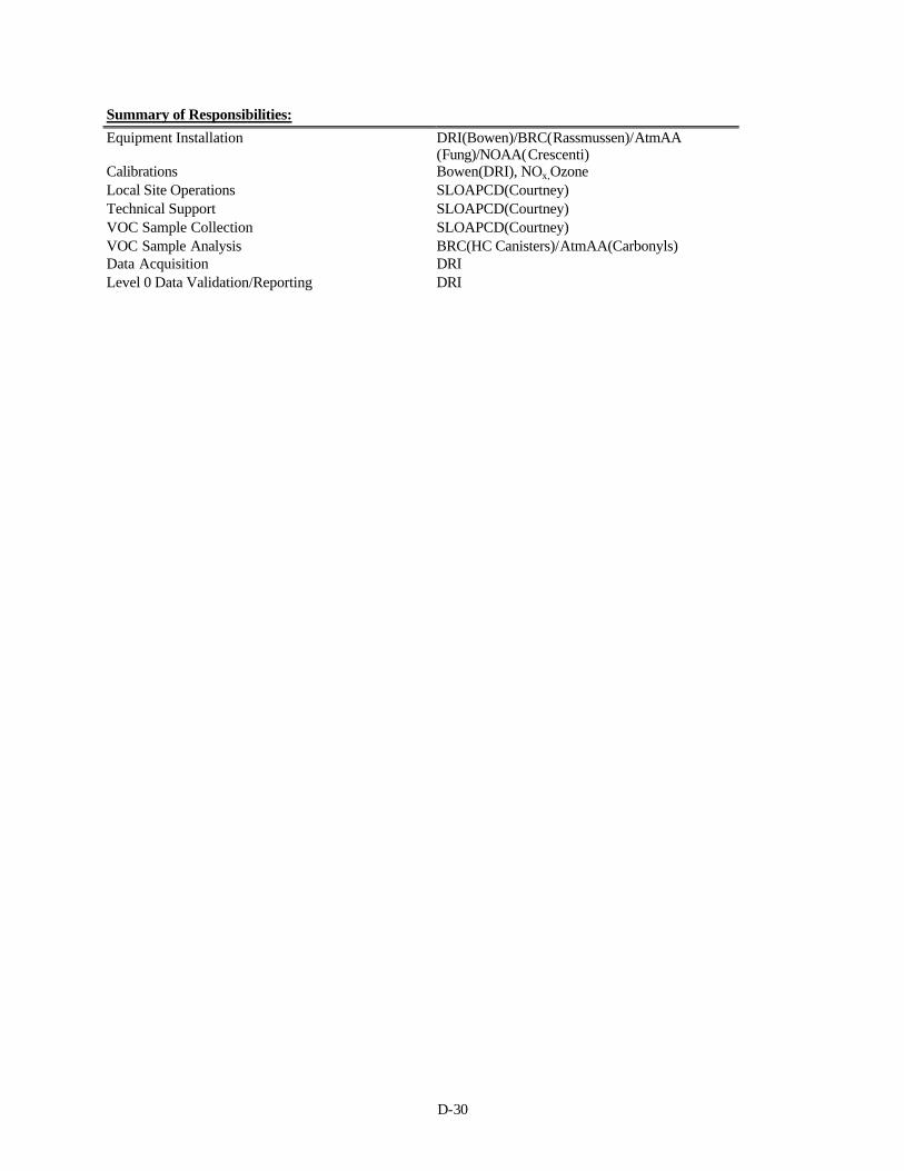
D-30
Summary of Responsibilities:
Equipment Installation DRI(Bowen)/BRC(Rassmussen)/AtmAA(Fung)/NOAA(Crescenti)
Calibrations Bowen(DRI), NOx,OzoneLocal Site Operations SLOAPCD(Courtney)Technical Support SLOAPCD(Courtney)VOC Sample Collection SLOAPCD(Courtney)VOC Sample Analysis BRC(HC Canisters)/AtmAA(Carbonyls)Data Acquisition DRILevel 0 Data Validation/Reporting DRI
D-31
Angiola (S1)
Address: 36078 4th Avenue, Corcoran, CA 93212
Location: From Corcoran, go south on Highway 43 to 4th, then south on 4th to intersection with TucsonAvenue, where site is. Look for 100m tower. It is about 7 miles south of the California St. Prisonon 4th.
Coordinates: Lat 35.9897 N Lon 119.4753 W
Elevation:
Description: Site is in cotton field area, with wide open exposure in all directions. Nearest road is 4th Avenue, anorth-south road ~ 100 yards to the east. Site includes 100m tower operated by SonomaTechnology Inc. for CRPAQS.
Local Contacts:
Name: Beth Wittig Organization: Sonoma Technology, Inc.Phone No: (661) 837-4219Email: [email protected]
NOTE: Site operations for CRPAQS are being done by STI. This includes O3 and NOy analyzers, whichoverlap with CCOS operations. For inquiries regarding CRPAQS operations being done by STI,consult Beth Wittig, as site operator.
Site Operator:Name: Beth WittigOrganization: Sonoma Technology Inc.Mailing Address: 2718 Ardee Circle, Bakersfield, CA 93304Shipping Address: SameOffice Phone: (661) 837-4219Cell Phone: (661) 203-1082Fax No: Same as office numberEmail: [email protected]
Site Phone: (559) 992-3794
Site Operator for Canister and Carbonyl SamplingName: Carl CampOrganization: San Joaquin Valley Unified APCDMailing Address: 1990 E. Gettysburg, Fresno, CA 93726Shipping Address: SameOffice Phone: (559) 230-5864
Existing Monitoring Equipment (vendor/model if available): This is an existing CRPAQS site, with 100m towerand extensive monitoring equipment for that study.
Angiola Supplemental Equipment:
Observable Instrument Installer
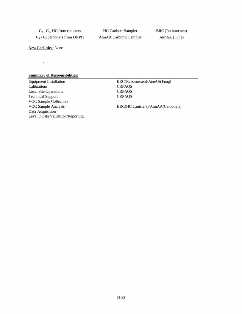
D-32
C2 - C12 HC from canisters HC Canister Sampler BRC (Rassmussen)
C1 - C7 carbonyls from DNPH AtmAA Carbonyl Sampler AtmAA (Fung)
New Facilities: None
.
Summary of Responsibilities:
Equipment Installation BRC(Rassmussen)/AtmAA(Fung)Calibrations CRPAQSLocal Site Operations CRPAQSTechnical Support CRPAQSVOC Sample CollectionVOC Sample Analysis BRC(HC Canisters)/AtmAA(Carbonyls)Data AcquisitionLevel 0 Data Validation/Reporting
D-33
Bethel Island (S2)
Address: 5551 Bethel Island Rd, Bethel Island
Location: From the town of Brentwood, go north on Highway 4 about 4 miles, then right on Cypress Road.Go 5 miles, at which point the road makes a sharp left and becomes Bethel Island Road. Justbefore the bridge, on the left, there is a boat self-storage building. (Don’t look for boats, as theyare inside the building). Instrument trailers are just north of the self-storage building.
Coordinates: Lat 38.0067 N, Lon 121.6414 W
Elevation: <5m
Description:
Local Contact:
Name: Tom Conwell, Area SupervisorTom will coordinate site operator training.
Organization: Bay Area AQMDPhone: (707) 552-3515Pager: (415) 998-9412
Name: Bob Franicevich, Senior AQ SpecialistBackup for Tom
Organization: Bay Area AQMDPhone No: (707) 553-8126
Site Operator:Name: Gary OwensOrganization: Bay Area AQMDMailing Address: BAAQMD(Also shipping) 939 Ellis St.
San Francisco, CA 94109Home Address 110 Mackie Dr.
Martinez, CA 94533
Office Phone: (925) 439-1303Pager: (415) 201-6675Fax No: (925) 439-1303 (regular line)Email: [email protected]
Backup OperatorName: Graham ScovellPhone: (925) 685-7947
Bethel Island Existing Equipment:
Observable Instrument
CO TECO Model 48Ozone TECO Model 49
NO/NO2/Nox TECO Model 42SO2 TECO Model 43A
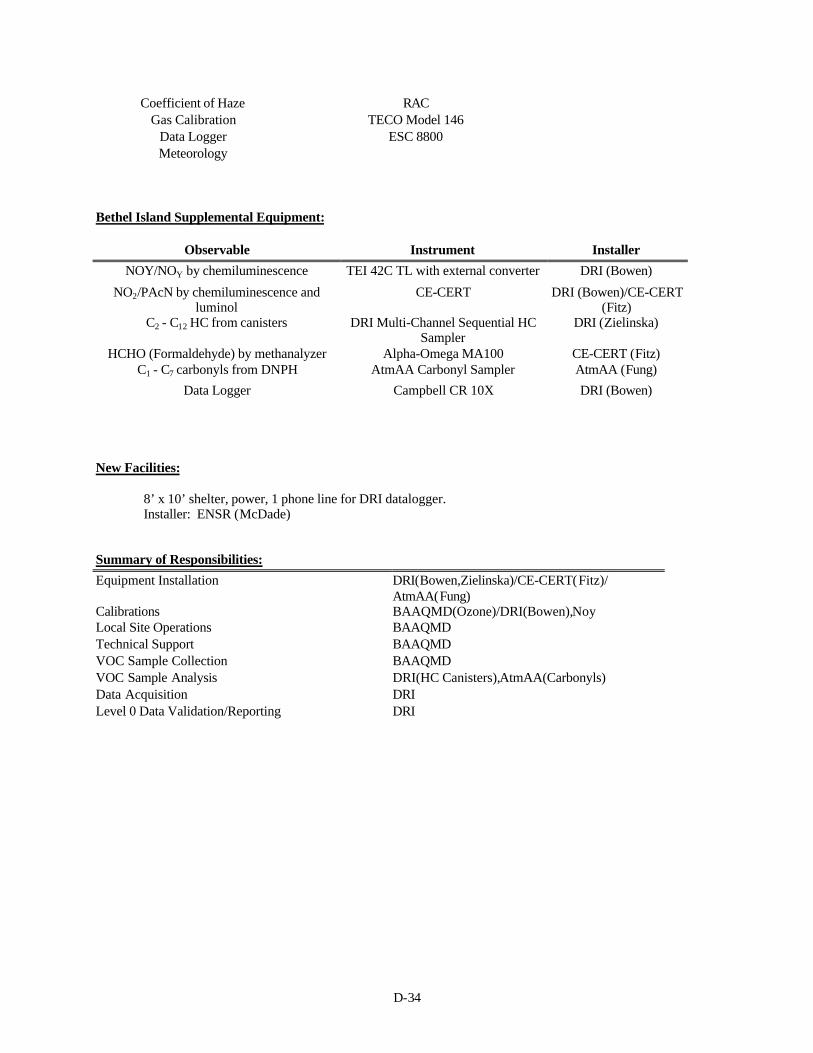
D-34
Coefficient of Haze RACGas Calibration TECO Model 146
Data Logger ESC 8800Meteorology
Bethel Island Supplemental Equipment:
Observable Instrument Installer
NOY/NOY by chemiluminescence TEI 42C TL with external converter DRI (Bowen)
NO2/PAcN by chemiluminescence andluminol
CE-CERT DRI (Bowen)/CE-CERT(Fitz)
C2 - C12 HC from canisters DRI Multi-Channel Sequential HCSampler
DRI (Zielinska)
HCHO (Formaldehyde) by methanalyzer Alpha-Omega MA100 CE-CERT (Fitz)C1 - C7 carbonyls from DNPH AtmAA Carbonyl Sampler AtmAA (Fung)
Data Logger Campbell CR 10X DRI (Bowen)
New Facilities:
8’ x 10’ shelter, power, 1 phone line for DRI datalogger.Installer: ENSR (McDade)
Summary of Responsibilities:
Equipment Installation DRI(Bowen,Zielinska)/CE-CERT(Fitz)/AtmAA(Fung)
Calibrations BAAQMD(Ozone)/DRI(Bowen),NoyLocal Site Operations BAAQMDTechnical Support BAAQMDVOC Sample Collection BAAQMDVOC Sample Analysis DRI(HC Canisters),AtmAA(Carbonyls)Data Acquisition DRILevel 0 Data Validation/Reporting DRI
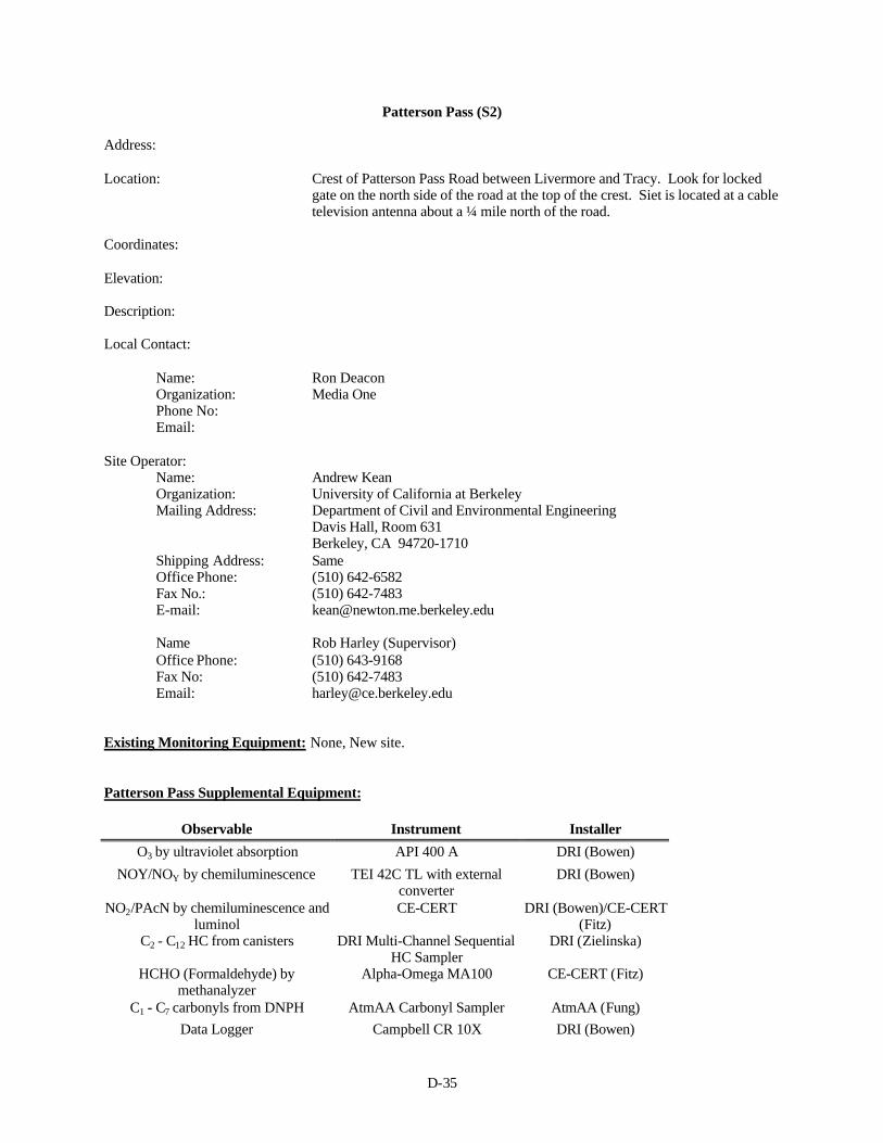
D-35
Patterson Pass (S2)
Address:
Location: Crest of Patterson Pass Road between Livermore and Tracy. Look for lockedgate on the north side of the road at the top of the crest. Siet is located at a cabletelevision antenna about a ¼ mile north of the road.
Coordinates:
Elevation:
Description:
Local Contact:
Name: Ron DeaconOrganization: Media OnePhone No:Email:
Site Operator:Name: Andrew KeanOrganization: University of California at BerkeleyMailing Address: Department of Civil and Environmental Engineering
Davis Hall, Room 631Berkeley, CA 94720-1710
Shipping Address: SameOffice Phone: (510) 642-6582Fax No.: (510) 642-7483E-mail: [email protected]
Name Rob Harley (Supervisor)Office Phone: (510) 643-9168Fax No: (510) 642-7483Email: [email protected]
Existing Monitoring Equipment: None, New site.
Patterson Pass Supplemental Equipment:
Observable Instrument Installer
O3 by ultraviolet absorption API 400 A DRI (Bowen)
NOY/NOY by chemiluminescence TEI 42C TL with externalconverter
DRI (Bowen)
NO2/PAcN by chemiluminescence andluminol
CE-CERT DRI (Bowen)/CE-CERT(Fitz)
C2 - C12 HC from canisters DRI Multi-Channel SequentialHC Sampler
DRI (Zielinska)
HCHO (Formaldehyde) bymethanalyzer
Alpha-Omega MA100 CE-CERT (Fitz)
C1 - C7 carbonyls from DNPH AtmAA Carbonyl Sampler AtmAA (Fung)
Data Logger Campbell CR 10X DRI (Bowen)
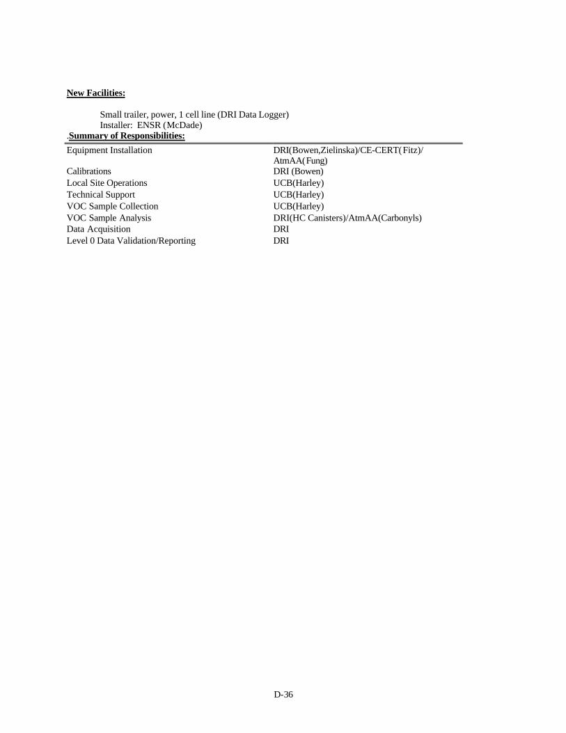
D-36
New Facilities:
Small trailer, power, 1 cell line (DRI Data Logger)Installer: ENSR (McDade)
.Summary of Responsibilities:
Equipment Installation DRI(Bowen,Zielinska)/CE-CERT(Fitz)/AtmAA(Fung)
Calibrations DRI (Bowen)Local Site Operations UCB(Harley)Technical Support UCB(Harley)VOC Sample Collection UCB(Harley)VOC Sample Analysis DRI(HC Canisters)/AtmAA(Carbonyls)Data Acquisition DRILevel 0 Data Validation/Reporting DRI
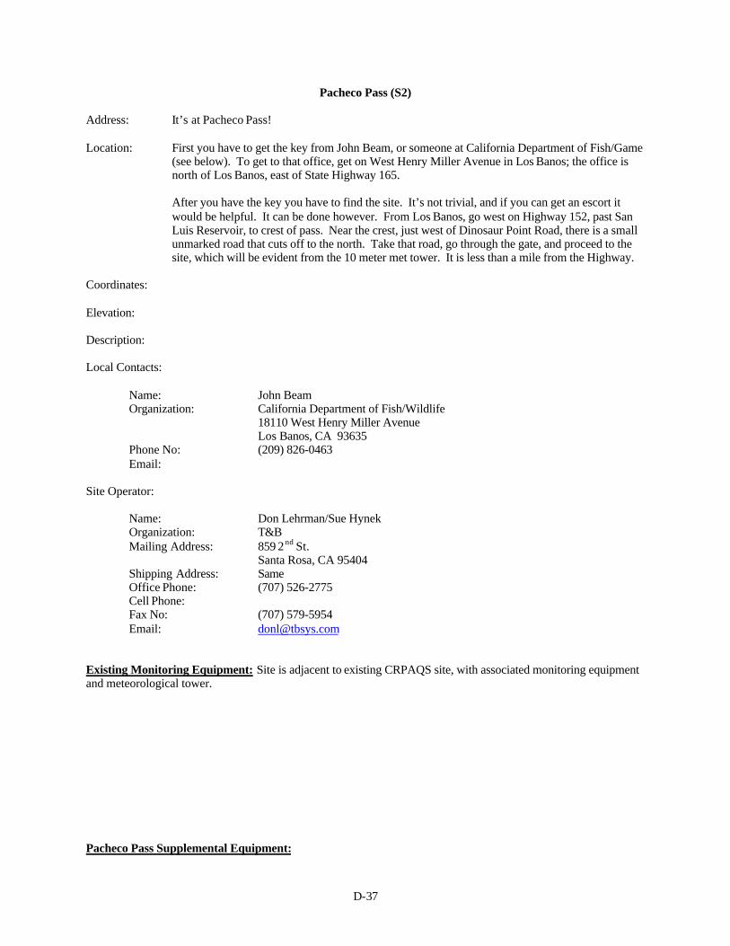
D-37
Pacheco Pass (S2)
Address: It’s at Pacheco Pass!
Location: First you have to get the key from John Beam, or someone at California Department of Fish/Game(see below). To get to that office, get on West Henry Miller Avenue in Los Banos; the office isnorth of Los Banos, east of State Highway 165.
After you have the key you have to find the site. It’s not trivial, and if you can get an escort itwould be helpful. It can be done however. From Los Banos, go west on Highway 152, past SanLuis Reservoir, to crest of pass. Near the crest, just west of Dinosaur Point Road, there is a smallunmarked road that cuts off to the north. Take that road, go through the gate, and proceed to thesite, which will be evident from the 10 meter met tower. It is less than a mile from the Highway.
Coordinates:
Elevation:
Description:
Local Contacts:
Name: John BeamOrganization: California Department of Fish/Wildlife
18110 West Henry Miller AvenueLos Banos, CA 93635
Phone No: (209) 826-0463Email:
Site Operator:
Name: Don Lehrman/Sue HynekOrganization: T&BMailing Address: 859 2 nd St.
Santa Rosa, CA 95404Shipping Address: SameOffice Phone: (707) 526-2775Cell Phone: Fax No: (707) 579-5954Email: [email protected]
Existing Monitoring Equipment: Site is adjacent to existing CRPAQS site, with associated monitoring equipmentand meteorological tower.
Pacheco Pass Supplemental Equipment:
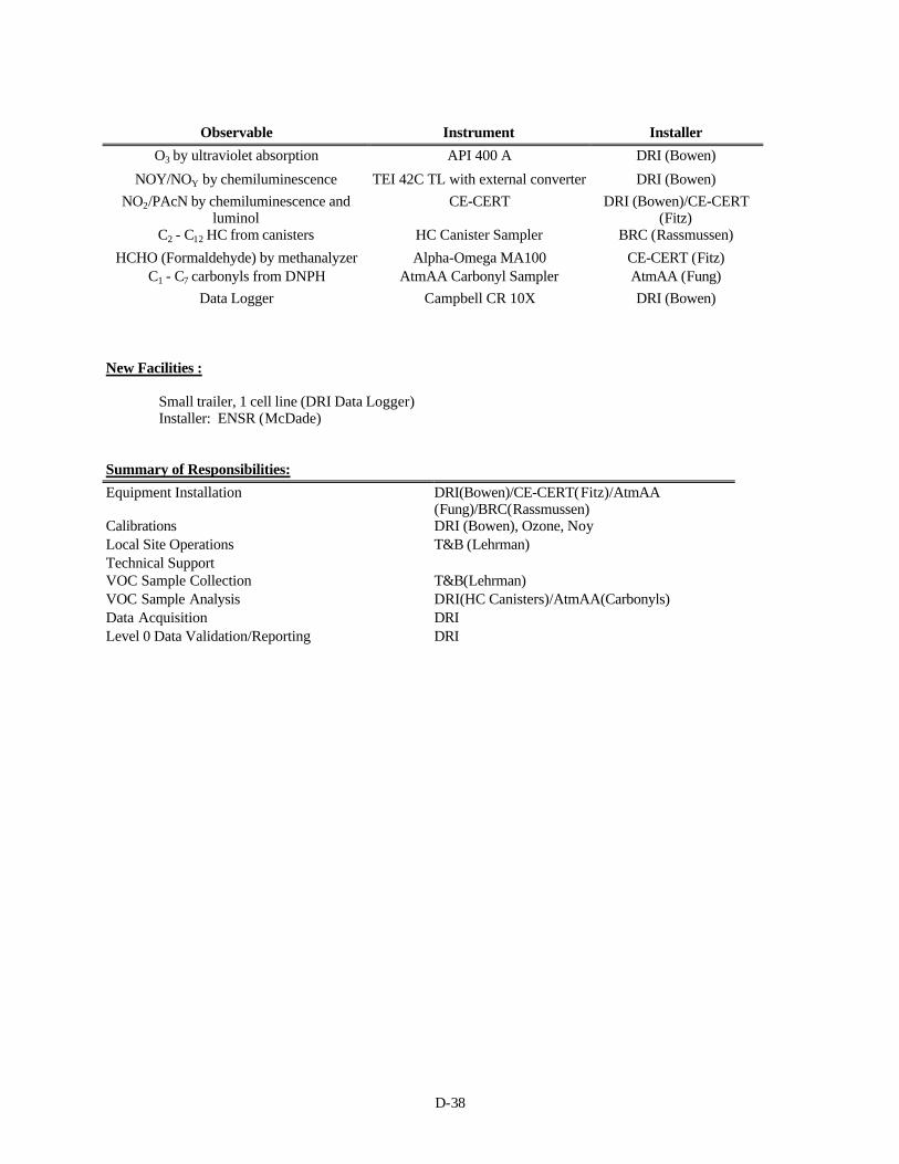
D-38
Observable Instrument Installer
O3 by ultraviolet absorption API 400 A DRI (Bowen)
NOY/NOY by chemiluminescence TEI 42C TL with external converter DRI (Bowen)
NO2/PAcN by chemiluminescence andluminol
CE-CERT DRI (Bowen)/CE-CERT(Fitz)
C2 - C12 HC from canisters HC Canister Sampler BRC (Rassmussen)
HCHO (Formaldehyde) by methanalyzer Alpha-Omega MA100 CE-CERT (Fitz)C1 - C7 carbonyls from DNPH AtmAA Carbonyl Sampler AtmAA (Fung)
Data Logger Campbell CR 10X DRI (Bowen)
New Facilities :
Small trailer, 1 cell line (DRI Data Logger)Installer: ENSR (McDade)
Summary of Responsibilities:
Equipment Installation DRI(Bowen)/CE-CERT(Fitz)/AtmAA(Fung)/BRC(Rassmussen)
Calibrations DRI (Bowen), Ozone, NoyLocal Site Operations T&B (Lehrman)Technical SupportVOC Sample Collection T&B(Lehrman)VOC Sample Analysis DRI(HC Canisters)/AtmAA(Carbonyls)Data Acquisition DRILevel 0 Data Validation/Reporting DRI
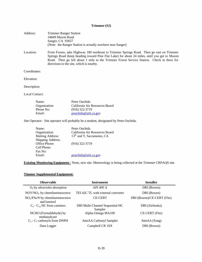
D-39
Trimmer (S2)
Address: Trimmer Ranger Station34849 Maxon RoadSanger, CA 93657(Note: the Ranger Station is actually nowhere near Sanger)
Location: From Fresno, take Highway 180 northeast to Trimmer Springs Road. Then go east on TrimmerSprings Road (keep heading toward Pine Flat Lake) for about 24 miles, until you get to MaxonRoad. Then go left about 1 mile to the Trimmer Forest Service Station. Check in there fordirections to the site, which is nearby.
Coordinates:
Elevation:
Description:
Local Contact:
Name: Peter OuchidaOrganization: California Air Resources BoardPhone No: (916) 322-3719Email: [email protected]
Site Operator: Site operator will probably be a student, designated by Peter Ouchida.
Name: Peter OuchidaOrganization: California Air Resources BoardMailing Address: 13th and T, Sacramento, CAShipping Address: Office Phone: (916) 322-3719Cell Phone: Fax No: Email: [email protected]
Existing Monitoring Equipment : None, new site. Meteorology is being collected at the Trimmer CRPAQS site.
Timmer Supplemental Equipment:
Observable Instrument Installer
O3 by ultraviolet absorption API 400 A DRI (Bowen)
NOY/NOY by chemiluminescence TEI 42C TL with external converter DRI (Bowen)
NO2/PAcN by chemiluminescenceand luminol
CE-CERT DRI (Bowen)/CE-CERT (Fitz)
C2 - C12 HC from canisters DRI Multi-Channel Sequential HCSampler
DRI (Zielinska)
HCHO (Formaldehyde) bymethanalyzer
Alpha-Omega MA100 CE-CERT (Fitz)
C1 - C7 carbonyls from DNPH AtmAA Carbonyl Sampler AtmAA (Fung)
Data Logger Campbell CR 10X DRI (Bowen)
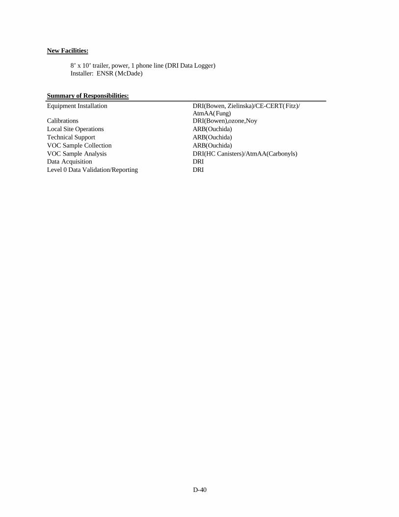
D-40
New Facilities:
8’ x 10’ trailer, power, 1 phone line (DRI Data Logger)Installer: ENSR (McDade)
Summary of Responsibilities:
Equipment Installation DRI(Bowen, Zielinska)/CE-CERT(Fitz)/AtmAA(Fung)
Calibrations DRI(Bowen),ozone,NoyLocal Site Operations ARB(Ouchida)Technical Support ARB(Ouchida)VOC Sample Collection ARB(Ouchida)VOC Sample Analysis DRI(HC Canisters)/AtmAA(Carbonyls)Data Acquisition DRILevel 0 Data Validation/Reporting DRI
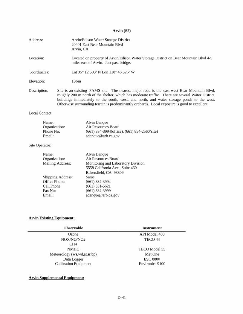
D-41
Arvin (S2)
Address: Arvin/Edison Water Storage District20401 East Bear Mountain BlvdArvin, CA
Location: Located on property of Arvin/Edison Water Storage District on Bear Mountain Blvd 4-5miles east of Arvin. Just past bridge.
Coordinates: Lat 35° 12.503’ N Lon 118° 46.526’ W
Elevation: 136m
Description: Site is an existing PAMS site. The nearest major road is the east-west Bear Mountain Blvd,roughly 200 m north of the shelter, which has moderate traffic. There are several Water Districtbuildings immediately to the south, west, and north, and water storage ponds to the west.Otherwise surrounding terrain is predominantly orchards. Local exposure is good to excellent.
Local Contact:
Name: Alvin DanqueOrganization: Air Resources BoardPhone No: (661) 334-3994(office), (661) 854-2560(site)Email: [email protected]
Site Operator:
Name: Alvin DanqueOrganization: Air Resources BoardMailing Address: Monitoring and Laboratory Division
5558 California Ave., Suite 460Bakersfield, CA 93309
Shipping Address: SameOffice Phone: (661) 334-3994Cell Phone: (661) 331-5621Fax No: (661) 334-3999Email: [email protected]
Arvin Existing Equipment:
Observable Instrument
Ozone API Model 400NOX/NO/NO2 TECO 44
CH4NMHC TECO Model 55
Meteorology (ws,wd,at,sr,bp) Met OneData Logger ESC 8800
Calibration Equipment Environics 9100
Arvin Supplemental Equipment:
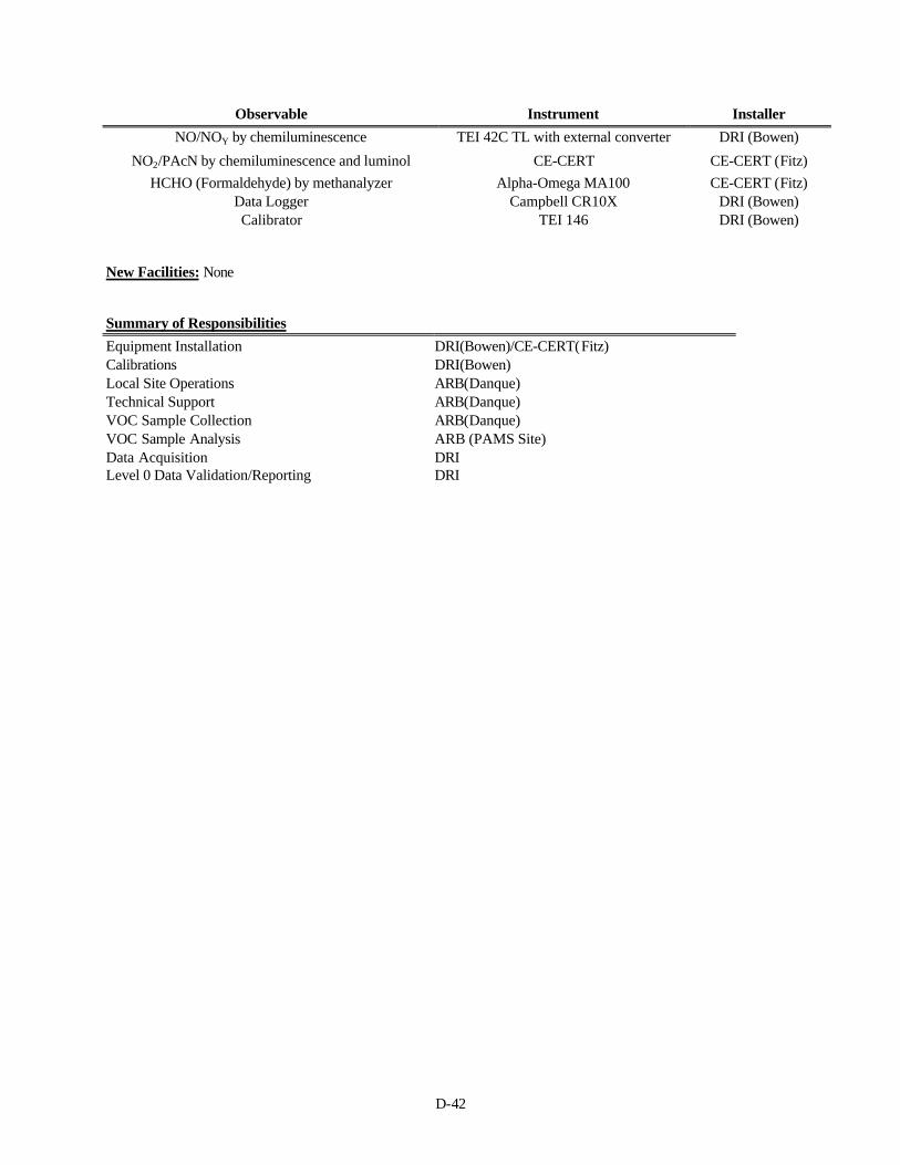
D-42
Observable Instrument Installer
NO/NOY by chemiluminescence TEI 42C TL with external converter DRI (Bowen)
NO2/PAcN by chemiluminescence and luminol CE-CERT CE-CERT (Fitz)
HCHO (Formaldehyde) by methanalyzer Alpha-Omega MA100 CE-CERT (Fitz)Data Logger Campbell CR10X DRI (Bowen)Calibrator TEI 146 DRI (Bowen)
New Facilities: None
Summary of Responsibilities
Equipment Installation DRI(Bowen)/CE-CERT(Fitz)Calibrations DRI(Bowen)Local Site Operations ARB(Danque)Technical Support ARB(Danque)VOC Sample Collection ARB(Danque)VOC Sample Analysis ARB (PAMS Site)Data Acquisition DRILevel 0 Data Validation/Reporting DRI
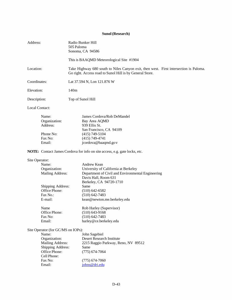
D-43
Sunol (Research)
Address: Radio Bunker Hill505 PalomaSonoma, CA 94586
This is BAAQMD Meteorological Site #1904
Location: Take Highway 680 south to Niles Canyon exit, then west. First intersection is Paloma.Go right. Access road to Sunol Hill is by General Store.
Coordinates: Lat 37.594 N, Lon 121.876 W
Elevation: 140m
Description: Top of Sunol Hill
Local Contact:
Name: James Cordova/Rob DeMandelOrganization: Bay Area AQMDAddress: 939 Ellis St.
San Francisco, CA 94109Phone No: (415) 749-5104Fax No: (415) 749-4741Email: [email protected]
NOTE: Contact James Cordova for info on site access, e.g. gate locks, etc.
Site Operator:Name: Andrew KeanOrganization: University of California at BerkeleyMailing Address: Department of Civil and Environmental Engineering
Davis Hall, Room 631Berkeley, CA 94720-1710
Shipping Address: SameOffice Phone: (510) 642-6582Fax No.: (510) 642-7483E-mail: [email protected]
Name Rob Harley (Supervisor)Office Phone: (510) 643-9168Fax No: (510) 642-7483Email: [email protected]
Site Operator (for GC/MS on IOPs):Name: John SagebielOrganization: Desert Research InstituteMailing Address: 2215 Raggio Parkway, Reno, NV 89512Shipping Address: SameOffice Phone: (775) 674-7064Cell Phone: Fax No: (775) 674-7060Email: [email protected]
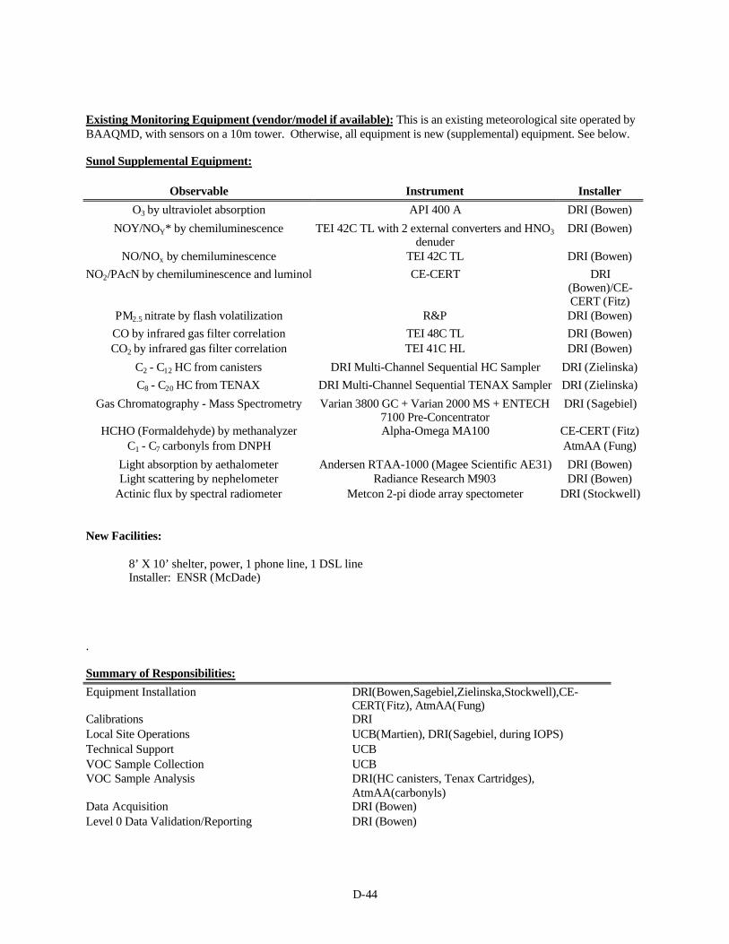
D-44
Existing Monitoring Equipment (vendor/model if available): This is an existing meteorological site operated byBAAQMD, with sensors on a 10m tower. Otherwise, all equipment is new (supplemental) equipment. See below.
Sunol Supplemental Equipment:
Observable Instrument Installer
O3 by ultraviolet absorption API 400 A DRI (Bowen)
NOY/NOY* by chemiluminescence TEI 42C TL with 2 external converters and HNO3
denuderDRI (Bowen)
NO/NOx by chemiluminescence TEI 42C TL DRI (Bowen)
NO2/PAcN by chemiluminescence and luminol CE-CERT DRI(Bowen)/CE-CERT (Fitz)
PM2.5 nitrate by flash volatilization R&P DRI (Bowen)
CO by infrared gas filter correlation TEI 48C TL DRI (Bowen)CO2 by infrared gas filter correlation TEI 41C HL DRI (Bowen)
C2 - C12 HC from canisters DRI Multi-Channel Sequential HC Sampler DRI (Zielinska)
C8 - C20 HC from TENAX DRI Multi-Channel Sequential TENAX Sampler DRI (Zielinska)
Gas Chromatography - Mass Spectrometry Varian 3800 GC + Varian 2000 MS + ENTECH7100 Pre-Concentrator
DRI (Sagebiel)
HCHO (Formaldehyde) by methanalyzer Alpha-Omega MA100 CE-CERT (Fitz)C1 - C7 carbonyls from DNPH AtmAA (Fung)
Light absorption by aethalometer Andersen RTAA-1000 (Magee Scientific AE31) DRI (Bowen)Light scattering by nephelometer Radiance Research M903 DRI (Bowen)
Actinic flux by spectral radiometer Metcon 2-pi diode array spectometer DRI (Stockwell)
New Facilities:
8’ X 10’ shelter, power, 1 phone line, 1 DSL lineInstaller: ENSR (McDade)
.
Summary of Responsibilities:
Equipment Installation DRI(Bowen,Sagebiel,Zielinska,Stockwell),CE-CERT(Fitz), AtmAA(Fung)
Calibrations DRILocal Site Operations UCB(Martien), DRI(Sagebiel, during IOPS)Technical Support UCBVOC Sample Collection UCBVOC Sample Analysis DRI(HC canisters, Tenax Cartridges),
AtmAA(carbonyls)Data Acquisition DRI (Bowen)Level 0 Data Validation/Reporting DRI (Bowen)
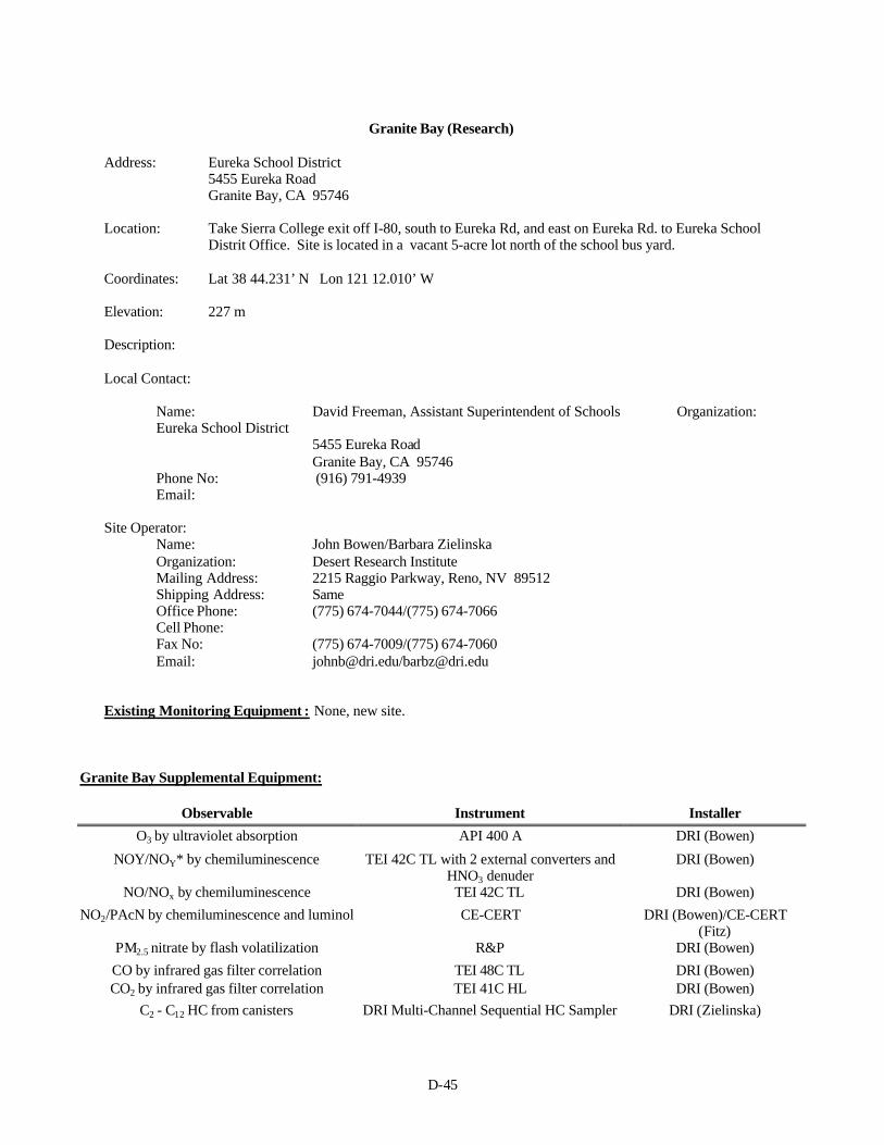
D-45
Granite Bay (Research)
Address: Eureka School District5455 Eureka RoadGranite Bay, CA 95746
Location: Take Sierra College exit off I-80, south to Eureka Rd, and east on Eureka Rd. to Eureka SchoolDistrit Office. Site is located in a vacant 5-acre lot north of the school bus yard.
Coordinates: Lat 38 44.231’ N Lon 121 12.010’ W
Elevation: 227 m
Description:
Local Contact:
Name: David Freeman, Assistant Superintendent of Schools Organization: Eureka School District
5455 Eureka RoadGranite Bay, CA 95746
Phone No: (916) 791-4939Email:
Site Operator:Name: John Bowen/Barbara ZielinskaOrganization: Desert Research InstituteMailing Address: 2215 Raggio Parkway, Reno, NV 89512Shipping Address: SameOffice Phone: (775) 674-7044/(775) 674-7066Cell Phone: Fax No: (775) 674-7009/(775) 674-7060Email: [email protected]/[email protected]
Existing Monitoring Equipment : None, new site.
Granite Bay Supplemental Equipment:
Observable Instrument Installer
O3 by ultraviolet absorption API 400 A DRI (Bowen)
NOY/NOY* by chemiluminescence TEI 42C TL with 2 external converters andHNO3 denuder
DRI (Bowen)
NO/NOx by chemiluminescence TEI 42C TL DRI (Bowen)
NO2/PAcN by chemiluminescence and luminol CE-CERT DRI (Bowen)/CE-CERT(Fitz)
PM2.5 nitrate by flash volatilization R&P DRI (Bowen)
CO by infrared gas filter correlation TEI 48C TL DRI (Bowen)CO2 by infrared gas filter correlation TEI 41C HL DRI (Bowen)
C2 - C12 HC from canisters DRI Multi-Channel Sequential HC Sampler DRI (Zielinska)
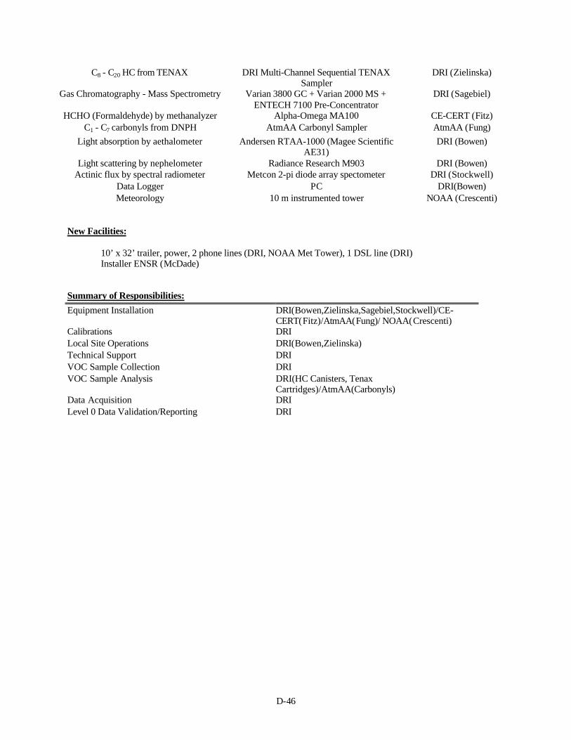
D-46
C8 - C20 HC from TENAX DRI Multi-Channel Sequential TENAXSampler
DRI (Zielinska)
Gas Chromatography - Mass Spectrometry Varian 3800 GC + Varian 2000 MS +ENTECH 7100 Pre-Concentrator
DRI (Sagebiel)
HCHO (Formaldehyde) by methanalyzer Alpha-Omega MA100 CE-CERT (Fitz)C1 - C7 carbonyls from DNPH AtmAA Carbonyl Sampler AtmAA (Fung)
Light absorption by aethalometer Andersen RTAA-1000 (Magee ScientificAE31)
DRI (Bowen)
Light scattering by nephelometer Radiance Research M903 DRI (Bowen)Actinic flux by spectral radiometer Metcon 2-pi diode array spectometer DRI (Stockwell)
Data Logger PC DRI(Bowen)Meteorology 10 m instrumented tower NOAA (Crescenti)
New Facilities:
10’ x 32’ trailer, power, 2 phone lines (DRI, NOAA Met Tower), 1 DSL line (DRI)Installer ENSR (McDade)
Summary of Responsibilities:
Equipment Installation DRI(Bowen,Zielinska,Sagebiel,Stockwell)/CE-CERT(Fitz)/AtmAA(Fung)/ NOAA(Crescenti)
Calibrations DRILocal Site Operations DRI(Bowen,Zielinska)Technical Support DRIVOC Sample Collection DRIVOC Sample Analysis DRI(HC Canisters, Tenax
Cartridges)/AtmAA(Carbonyls)Data Acquisition DRILevel 0 Data Validation/Reporting DRI
D-47
Parlier (Research)
Address: Kearney Agricultural Research Station9240 South Riverbend AvenueParlier, CA 93648
Location: From Parlier, one block east on Manning, then right onto Riverbend, then secondentrance on left. Contact Richard Nelson (below) for access.
Coordinates: Lat 36 35 51 N Lon 119 30 13 W
Elevation:
Description:
Local Contacts:Name: Fred Swanson, SuperintendentOrganization: Kearney Agricultural Research StationPhone No: (559) 646-6060Email: [email protected]
Name: John Gallup/Evan ShippOrganization: San Joaquin Valley Unified APCDPhone No: (559) 230-5860/(559) 230-5809Email: [email protected]/[email protected]
Site Operator:Name: Richard NelsonOrganization: San Joaquin Valley Unified APCDMailing Address: 1990 East Gettysburg Avenue, Fresno, CA 93726-0244Shipping Address: SameOffice Phone: (559) 230-5863Cell Phone: NoneFax No: (559) 230-6064Email: [email protected]
Site Operator (for GC/MS on IOPs):Name: Mark McDanielOrganization: Desert Research InstituteMailing Address: 2215 Raggio Parkway, Reno, NV 89512Shipping Address: SameOffice Phone: (775) 674-7180Cell Phone: Fax No: (775) 674-7060Email: [email protected]
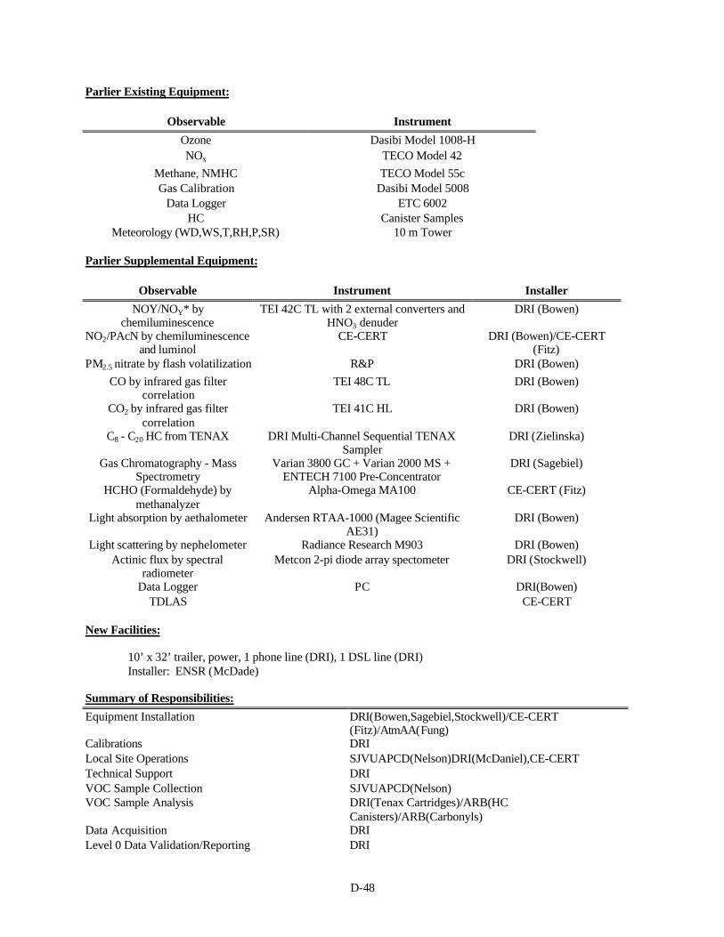
D-48
Parlier Existing Equipment:
Observable Instrument
Ozone Dasibi Model 1008-HNOx TECO Model 42
Methane, NMHC TECO Model 55cGas Calibration Dasibi Model 5008
Data Logger ETC 6002HC Canister Samples
Meteorology (WD,WS,T,RH,P,SR) 10 m Tower
Parlier Supplemental Equipment:
Observable Instrument Installer
NOY/NOY* bychemiluminescence
TEI 42C TL with 2 external converters andHNO3 denuder
DRI (Bowen)
NO2/PAcN by chemiluminescenceand luminol
CE-CERT DRI (Bowen)/CE-CERT(Fitz)
PM2.5 nitrate by flash volatilization R&P DRI (Bowen)
CO by infrared gas filtercorrelation
TEI 48C TL DRI (Bowen)
CO2 by infrared gas filtercorrelation
TEI 41C HL DRI (Bowen)
C8 - C20 HC from TENAX DRI Multi-Channel Sequential TENAXSampler
DRI (Zielinska)
Gas Chromatography - MassSpectrometry
Varian 3800 GC + Varian 2000 MS +ENTECH 7100 Pre-Concentrator
DRI (Sagebiel)
HCHO (Formaldehyde) bymethanalyzer
Alpha-Omega MA100 CE-CERT (Fitz)
Light absorption by aethalometer Andersen RTAA-1000 (Magee ScientificAE31)
DRI (Bowen)
Light scattering by nephelometer Radiance Research M903 DRI (Bowen)Actinic flux by spectral
radiometerMetcon 2-pi diode array spectometer DRI (Stockwell)
Data Logger PC DRI(Bowen)TDLAS CE-CERT
New Facilities:
10’ x 32’ trailer, power, 1 phone line (DRI), 1 DSL line (DRI)Installer: ENSR (McDade)
Summary of Responsibilities:
Equipment Installation DRI(Bowen,Sagebiel,Stockwell)/CE-CERT(Fitz)/AtmAA(Fung)
Calibrations DRILocal Site Operations SJVUAPCD(Nelson)DRI(McDaniel),CE-CERTTechnical Support DRIVOC Sample Collection SJVUAPCD(Nelson)VOC Sample Analysis DRI(Tenax Cartridges)/ARB(HC
Canisters)/ARB(Carbonyls)Data Acquisition DRILevel 0 Data Validation/Reporting DRI
D-49
Shasta Lake (Other)
Address: Shasta Lake Fire District13791 Lake BlvdShasta Lake, CA 96019
Location: From I5, take the State Highway 151 (Shasta Dam Blvd) exit. Go west ~ 4 miles to intersectionwith Lake Blvd. Turn south, go a short distance to the Fire District office on the east side of LakeBlvd.
This is a new site to be operated by Shasta AQMD. Equipment is located in an air-conditionedgarage at the Fire Protection District facility. Contact Rita Cirulis for access.
Coordinates: Lat 40° 41.37’ N, Lat 122° 24.14’ W
Elevation: 361 m
Description: Residential
Local Contact:Name: Charles E. Dahlen, Battalion Chief/Fire MarshalOrganization: Shasta Lake Fire Protection District
4126 Ashby CourtShasta Lake, CA 96019-9215
Phone No: (530) 275-7474Fax No: (530) 275-6502Email: [email protected]
Site Operator:Name: Rita CirulisOrganization: Shasta AQMDMailing Address: 1855 Placer St., Suite 101, Redding CA 96001Shipping Address: SameOffice Phone: (530) 225-5156, or 225-5674Cell Phone: NoneFax No: (530) 225-5237Email: [email protected]
Existing Monitoring Equipment: Ozone (Dasibi 1003), meteorology on 10m tower.
Supplemental Monitoring Equipment:
New Facilities:
Responsibilities: Shasta AQMD is responsible for this site.
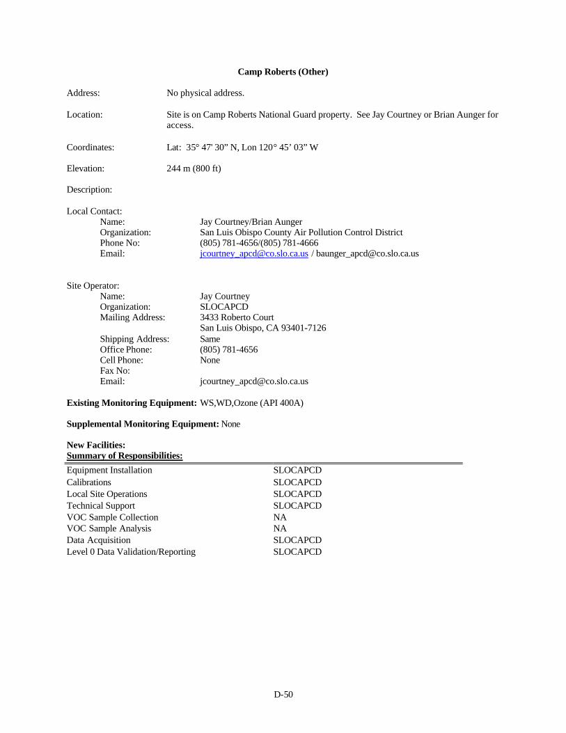
D-50
Camp Roberts (Other)
Address: No physical address.
Location: Site is on Camp Roberts National Guard property. See Jay Courtney or Brian Aunger foraccess.
Coordinates: Lat: 35° 47' 30” N, Lon 120° 45’ 03” W
Elevation: 244 m (800 ft)
Description:
Local Contact:Name: Jay Courtney/Brian AungerOrganization: San Luis Obispo County Air Pollution Control DistrictPhone No: (805) 781-4656/(805) 781-4666Email: [email protected] / [email protected]
Site Operator:Name: Jay CourtneyOrganization: SLOCAPCDMailing Address: 3433 Roberto Court
San Luis Obispo, CA 93401-7126Shipping Address: SameOffice Phone: (805) 781-4656Cell Phone: NoneFax No: Email: [email protected]
Existing Monitoring Equipment: WS,WD,Ozone (API 400A)
Supplemental Monitoring Equipment: None
New Facilities:Summary of Responsibilities:
Equipment Installation SLOCAPCDCalibrations SLOCAPCDLocal Site Operations SLOCAPCDTechnical Support SLOCAPCDVOC Sample Collection NAVOC Sample Analysis NAData Acquisition SLOCAPCDLevel 0 Data Validation/Reporting SLOCAPCD
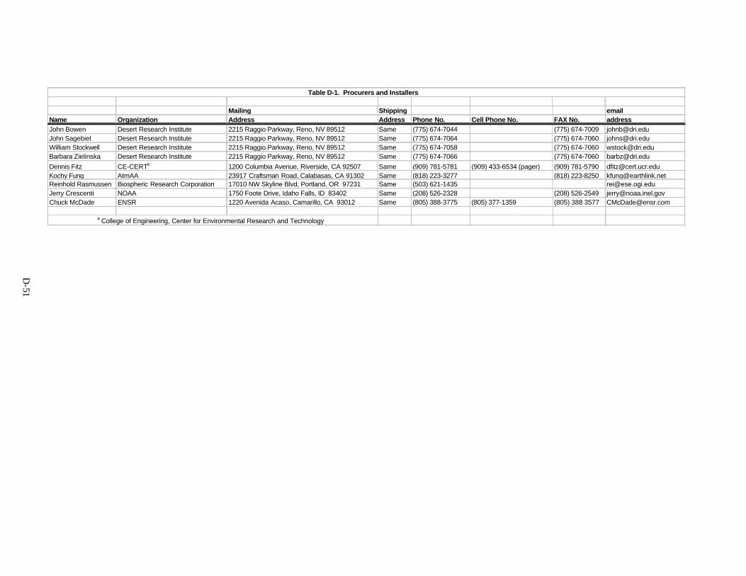
D-51
Table D-1. Procurers and Installers
Mailing Shipping emailName Organization Address Address Phone No. Cell Phone No. FAX No. addressJohn Bowen Desert Research Institute 2215 Raggio Parkway, Reno, NV 89512 Same (775) 674-7044 (775) 674-7009 [email protected] Sagebiel Desert Research Institute 2215 Raggio Parkway, Reno, NV 89512 Same (775) 674-7064 (775) 674-7060 [email protected] Stockwell Desert Research Institute 2215 Raggio Parkway, Reno, NV 89512 Same (775) 674-7058 (775) 674-7060 [email protected] Zielinska Desert Research Institute 2215 Raggio Parkway, Reno, NV 89512 Same (775) 674-7066 (775) 674-7060 [email protected]
Dennis Fitz CE-CERTa 1200 Columbia Avenue, Riverside, CA 92507 Same (909) 781-5781 (909) 433-6534 (pager) (909) 781-5790 [email protected] Fung AtmAA 23917 Craftsman Road, Calabasas, CA 91302 Same (818) 223-3277 (818) 223-8250 [email protected] Rasmussen Biospheric Research Corporation 17010 NW Skyline Blvd, Portland, OR 97231 Same (503) 621-1435 [email protected] Crescenti NOAA 1750 Foote Drive, Idaho Falls, ID 83402 Same (208) 526-2328 (208) 526-2549 [email protected] McDade ENSR 1220 Avenida Acaso, Camarillo, CA 93012 Same (805) 388-3775 (805) 377-1359 (805) 388 3577 [email protected]
a College of Engineering, Center for Environmental Research and Technology
Appendix D-2
Supplemental Air Quality Site Descriptions and Installation Information
Site Photos
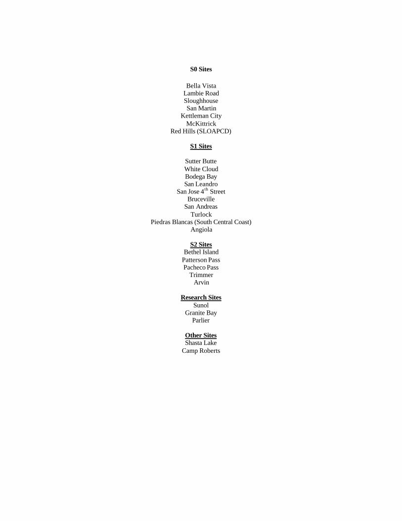
S0 Sites
Bella VistaLambie RoadSloughhouseSan Martin
Kettleman CityMcKittrick
Red Hills (SLOAPCD)
S1 Sites
Sutter ButteWhite CloudBodega BaySan Leandro
San Jose 4th StreetBruceville
San AndreasTurlock
Piedras Blancas (South Central Coast)Angiola
S2 SitesBethel Island
Patterson PassPacheco Pass
TrimmerArvin
Research SitesSunol
Granite BayParlier
Other SitesShasta Lake
Camp Roberts
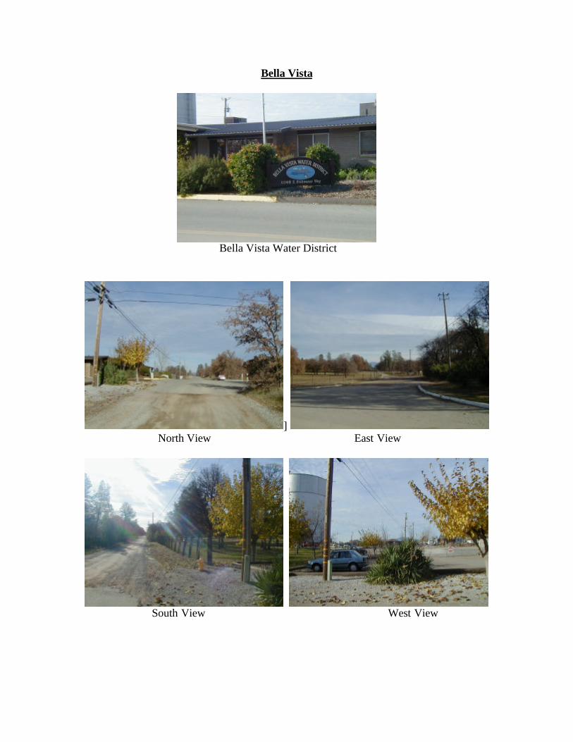
Bella Vista
Bella Vista Water District
] North View East View
South View West View
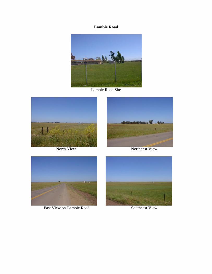
Lambie Road
Lambie Road Site
North View Northeast View
East View on Lambie Road Southeast View
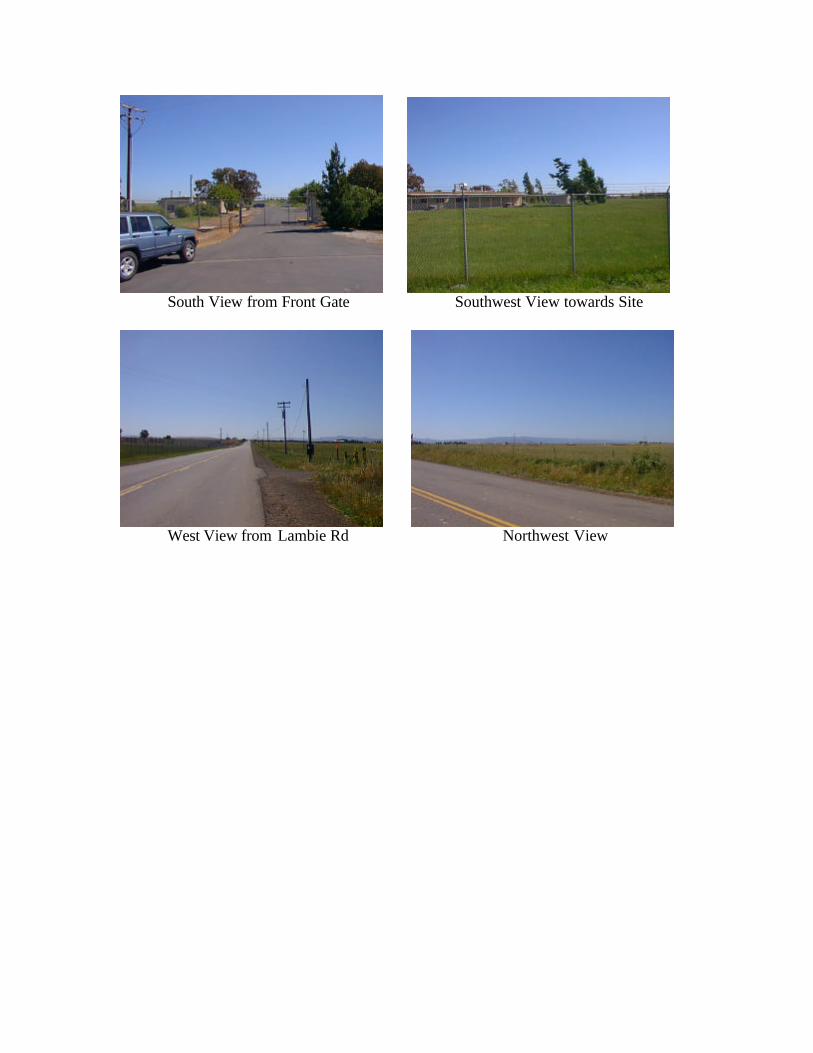
South View from Front Gate Southwest View towards Site
West View from Lambie Rd Northwest View
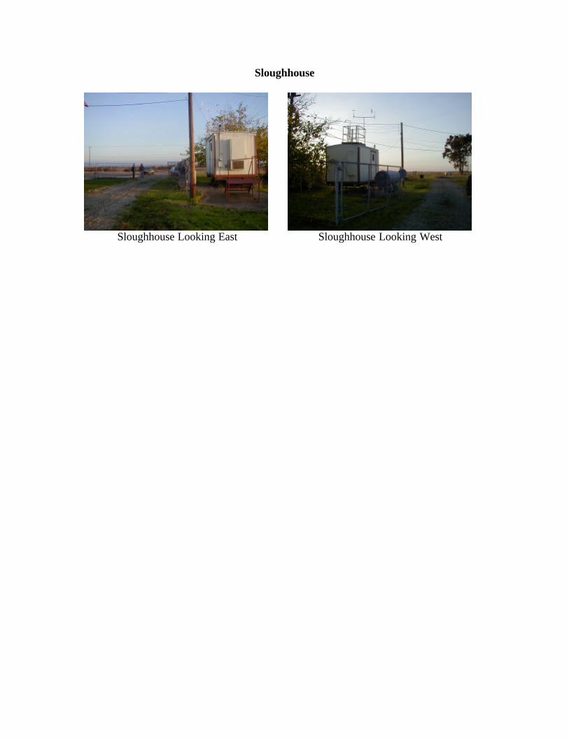
Sloughhouse
Sloughhouse Looking East Sloughhouse Looking West
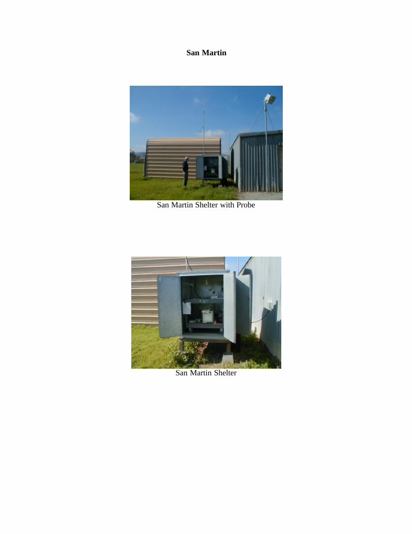
San Martin
San Martin Shelter with Probe
San Martin Shelter
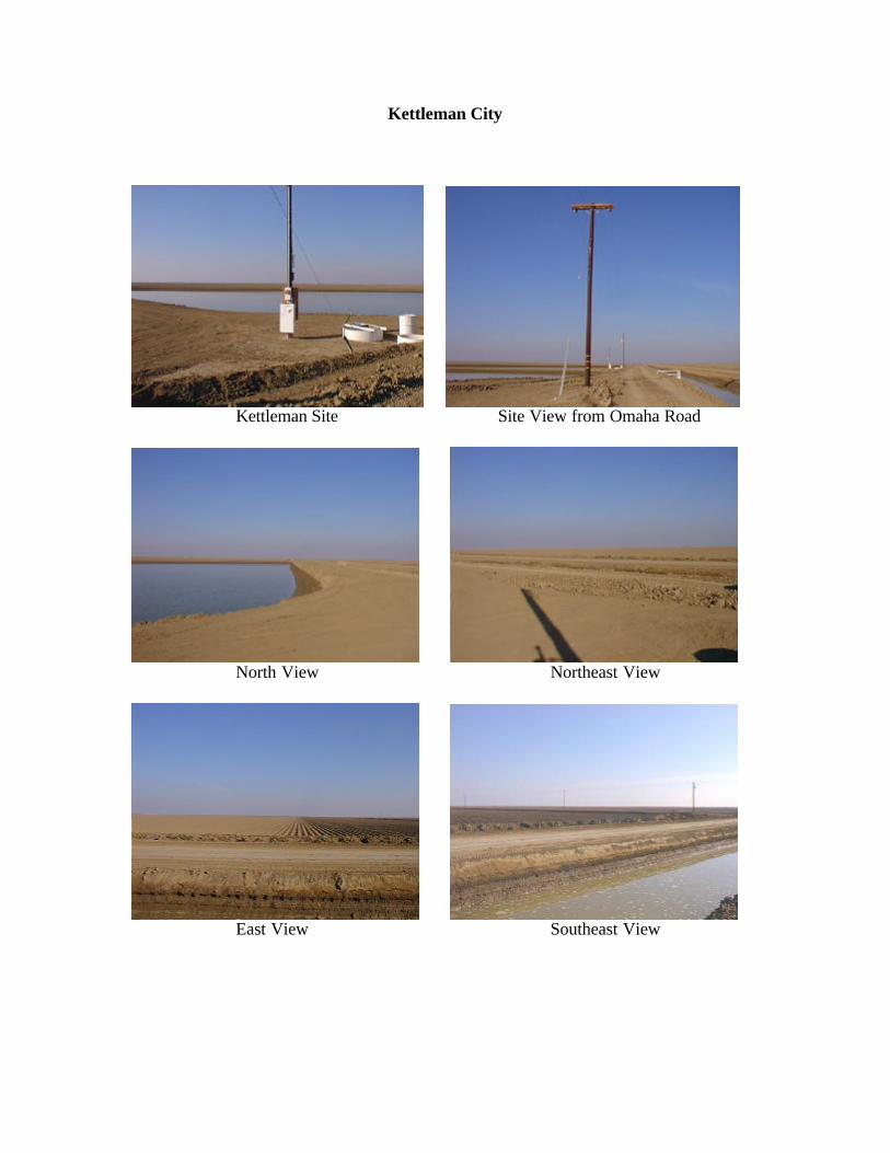
Kettleman City
Kettleman Site Site View from Omaha Road
North View Northeast View
East View Southeast View
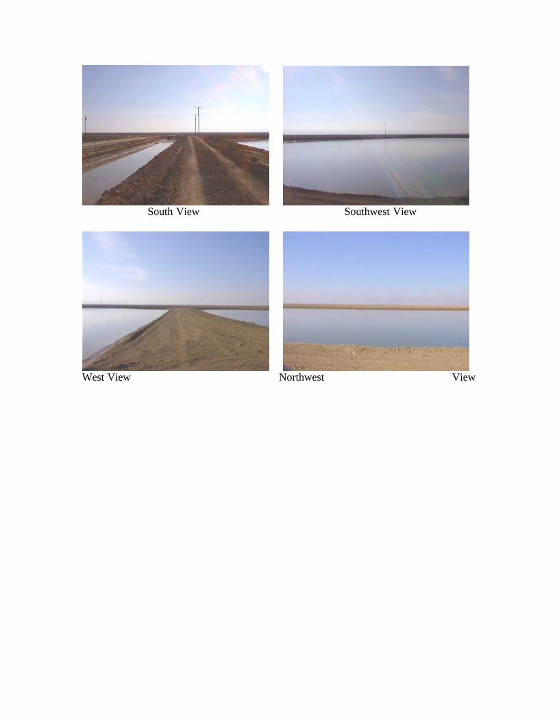
South View Southwest View
West View Northwest View
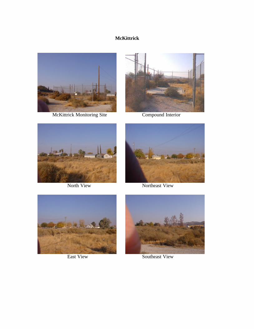
McKittrick
McKittrick Monitoring Site Compound Interior
North View Northeast View
East View Southeast View
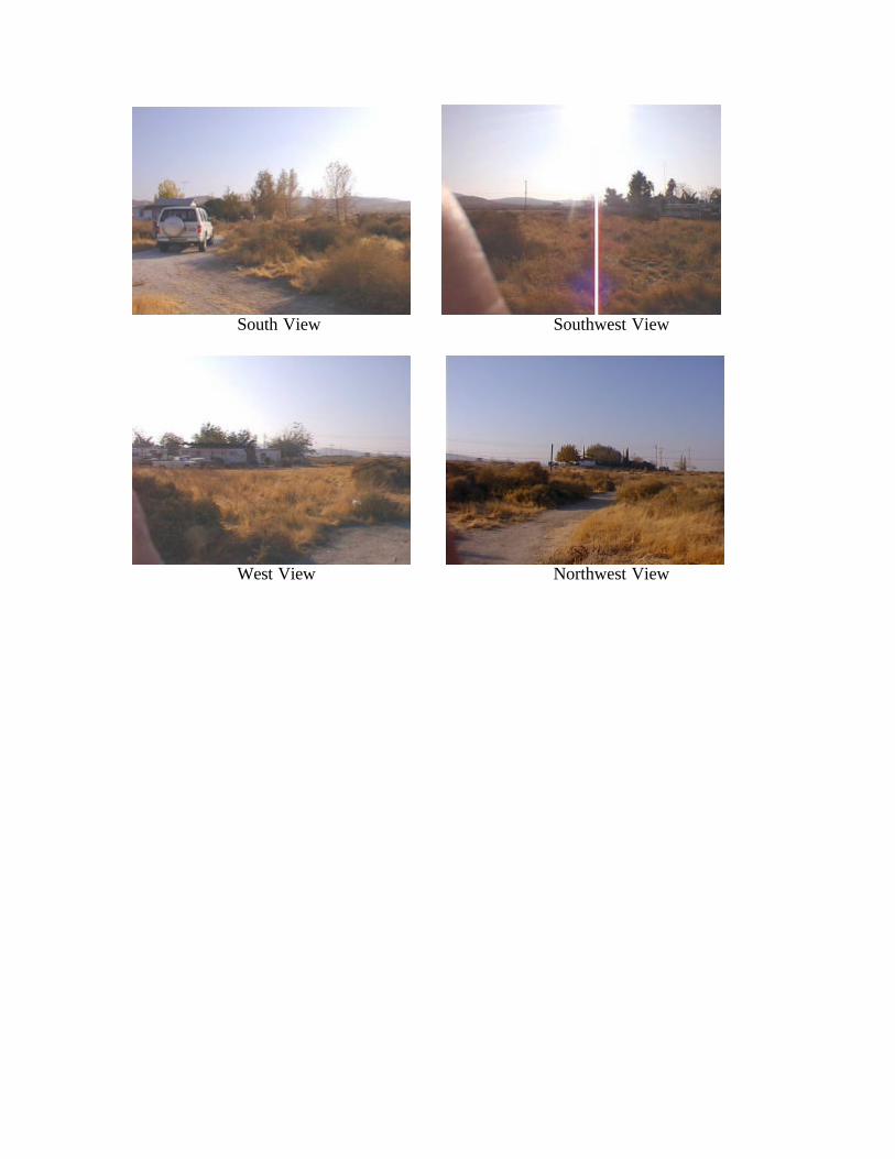
South View Southwest View
West View Northwest View

Red Hills

Sutter Butte
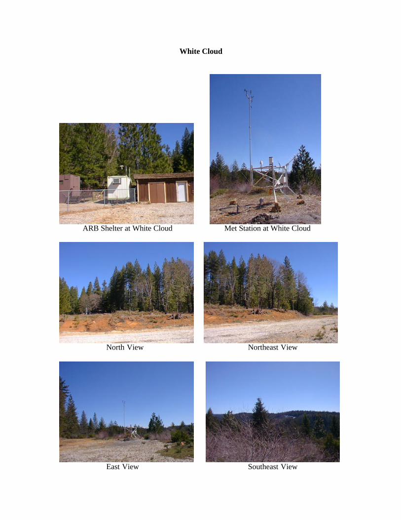
White Cloud
ARB Shelter at White Cloud Met Station at White Cloud
North View Northeast View
East View Southeast View
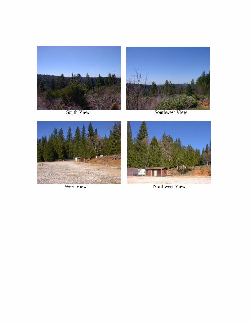
South View Southwest View
West View Northwest View
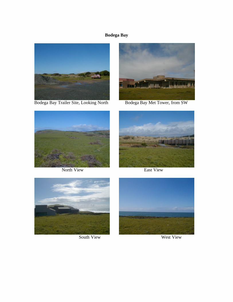
Bodega Bay
Bodega Bay Trailer Site, Looking North Bodega Bay Met Tower, from SW
North View East View
South View West View

San Leandro

San Jose 4th Street

Bruceville
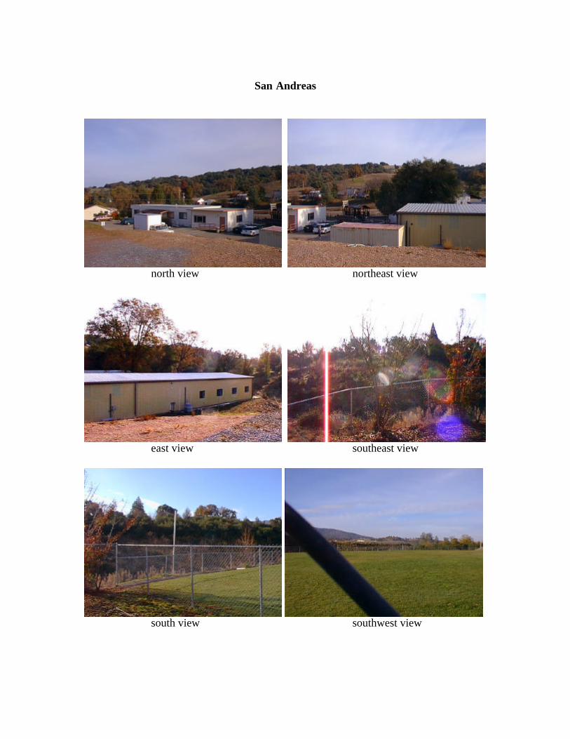
San Andreas
north view northeast view
east view southeast view
south view southwest view
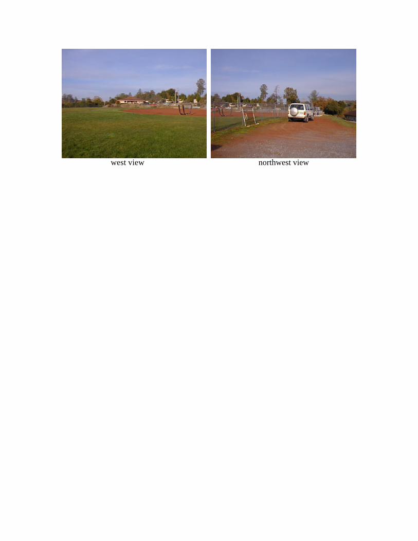
west view northwest view
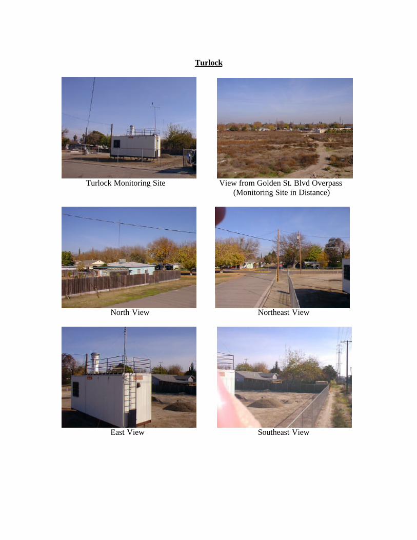
Turlock
Turlock Monitoring Site View from Golden St. Blvd Overpass
(Monitoring Site in Distance)
North View Northeast View
East View Southeast View
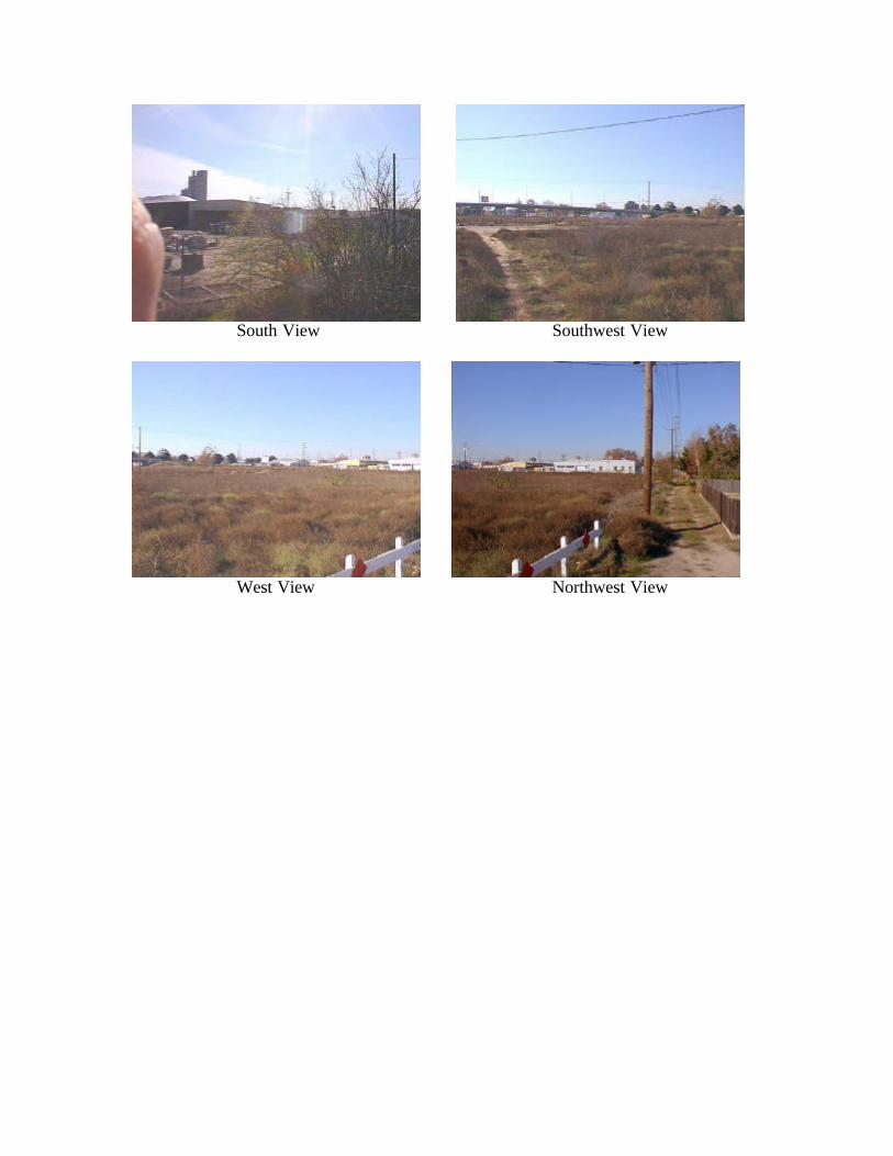
South View Southwest View
West View Northwest View
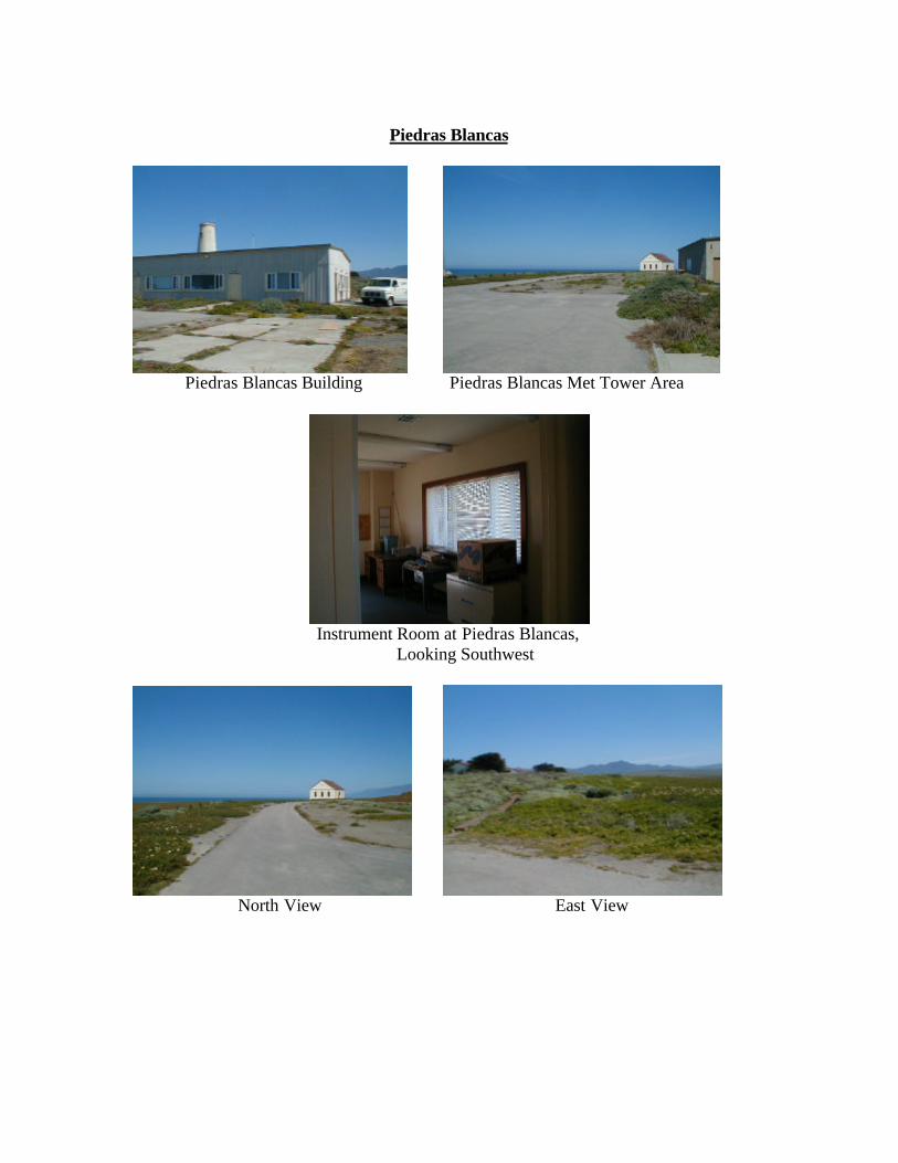
Piedras Blancas
Piedras Blancas Building Piedras Blancas Met Tower Area
Instrument Room at Piedras Blancas,Looking Southwest
North View East View
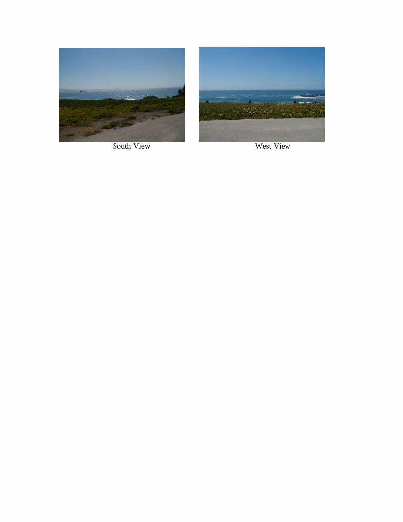
South View West View
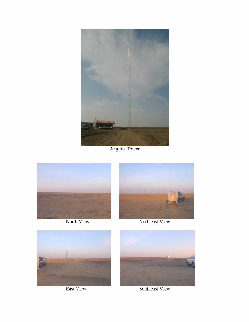
Angiola Tower
North View Northeast View
East View Southeast View
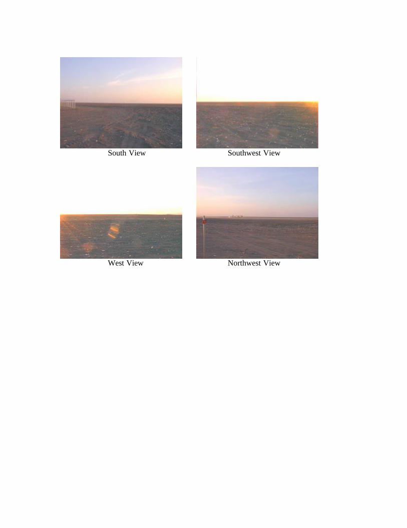
South View Southwest View
West View Northwest View
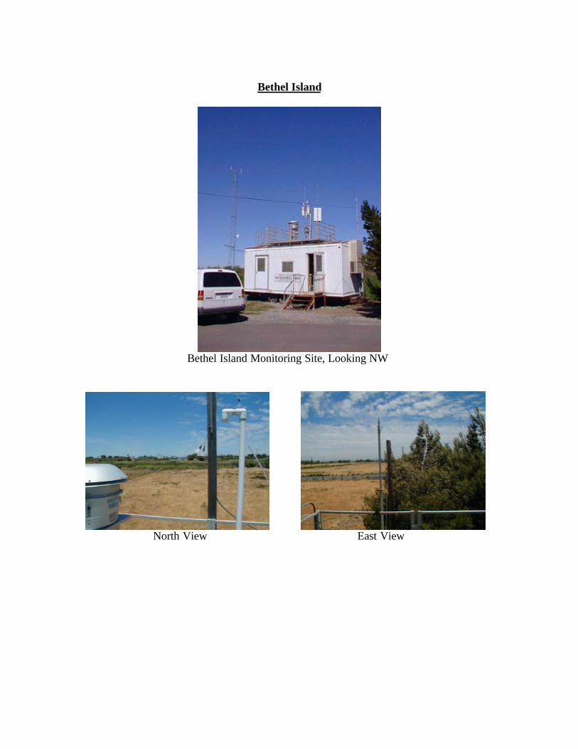
Bethel Island
Bethel Island Monitoring Site, Looking NW
North View East View
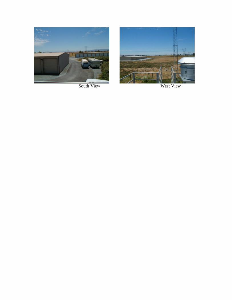
South View West View

Patterson Pass
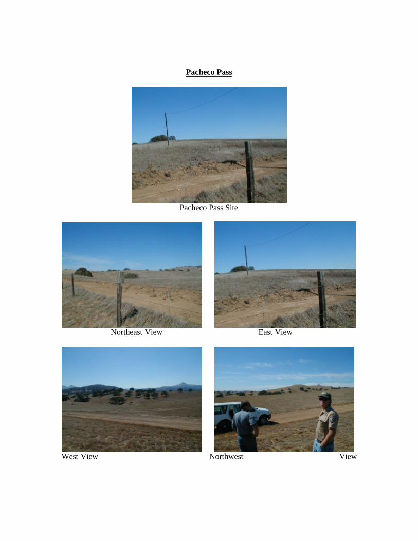
Pacheco Pass
Pacheco Pass Site
Northeast View East View
West View Northwest View
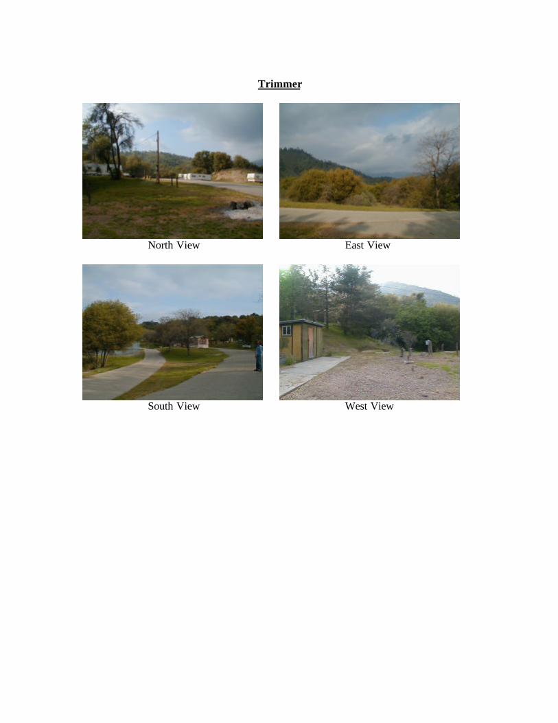
Trimmer
North View East View
South View West View
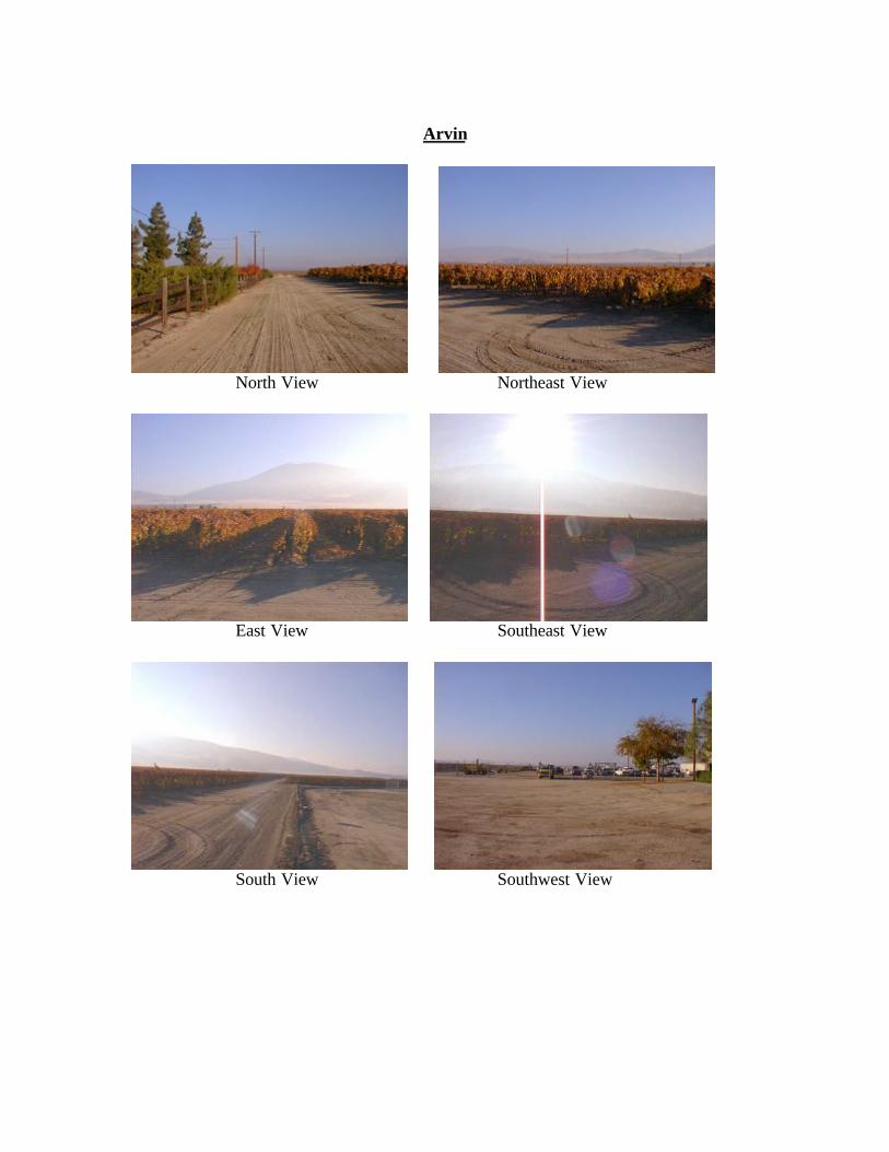
Arvin
North View Northeast View
East View Southeast View
South View Southwest View
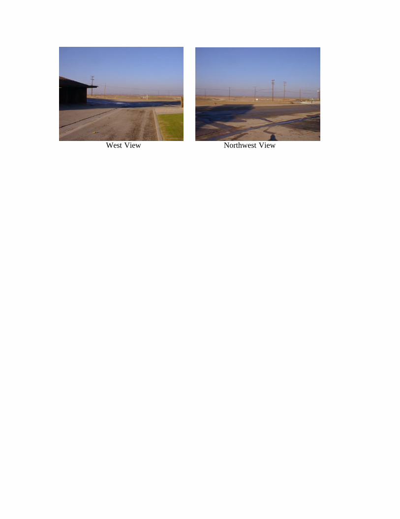
West View Northwest View
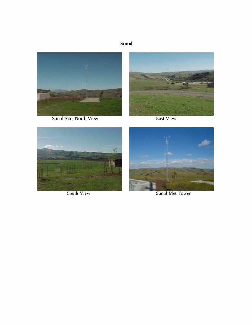
Sunol
Sunol Site, North View East View
South View Sunol Met Tower
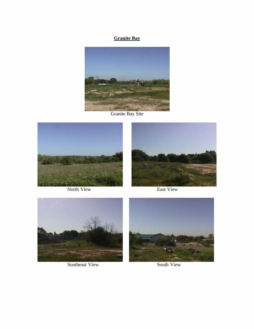
Granite Bay
Granite Bay Site
North View East View
Southeast View South View
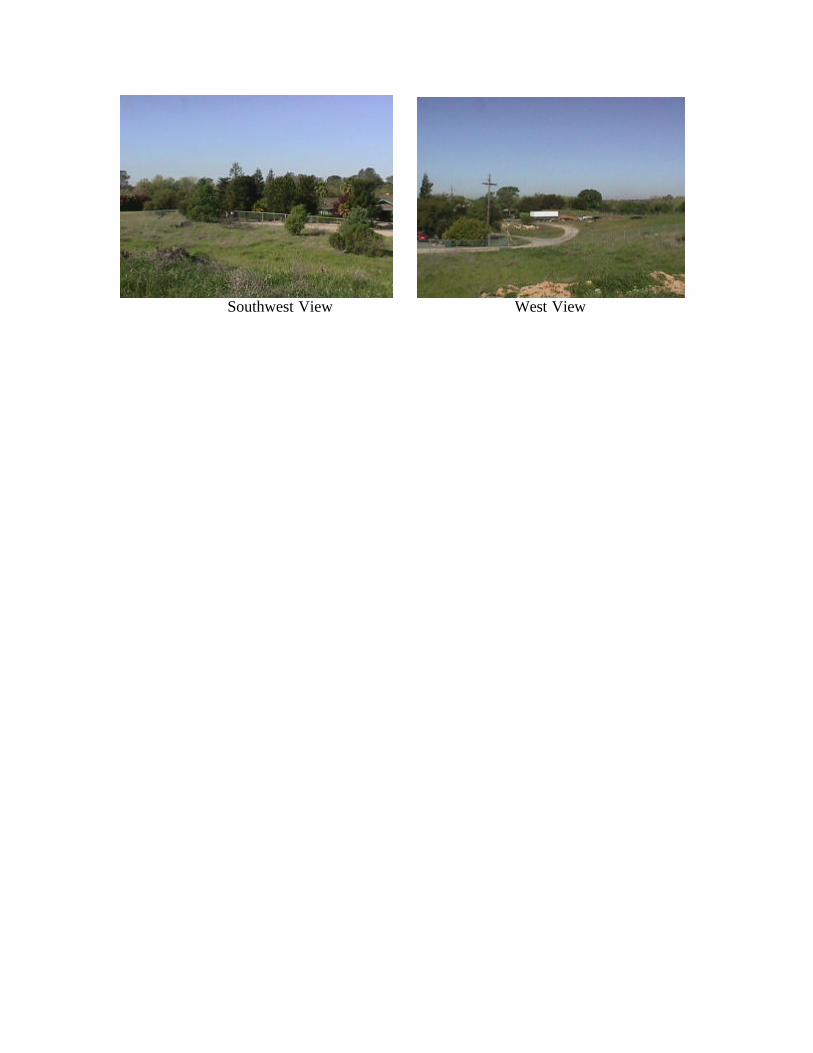
Southwest View West View

Parlier
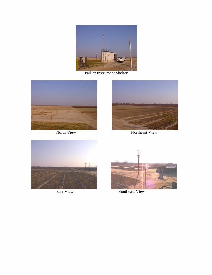
Parlier Instrument Shelter
North View Northeast View
East View Southeast View
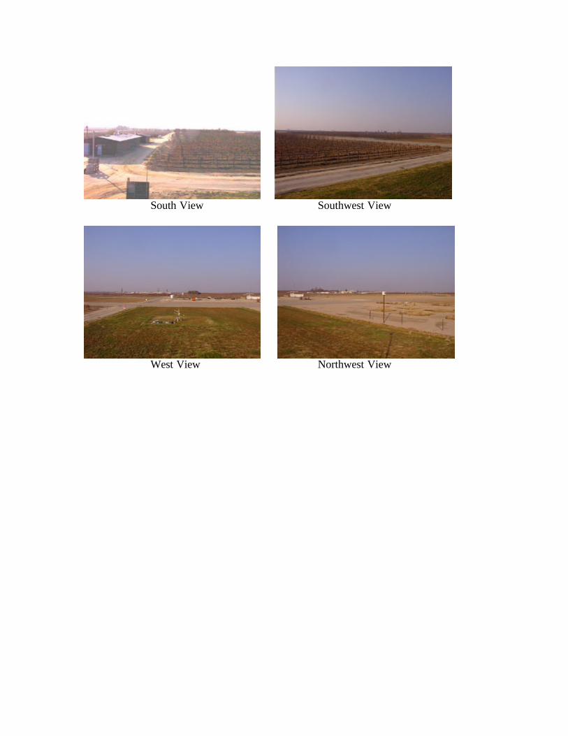
South View Southwest View
West View Northwest View
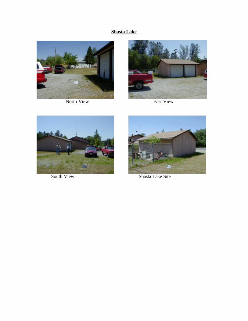
Shasta Lake
North View East View
South View Shasta Lake Site

Camp Roberts