Embed Size (px)
Citation preview

MEASUREMENTS MADE ALOFT BYTWO AIRCRAFT TO SUPPORT THE
CENTRAL CALIFORNIA OZONE STUDY(CCOS)
FINAL REPORTSTI-900106-2131-DFR
By:Martin P. Buhr
Donald L. Blumenthal*Siana H. Alcorn
*Principal Investigator
Sonoma Technology, Inc.1360 Redwood Way, Suite C
Petaluma, CA 94954-1169
Prepared for:San Joaquin Valleywide Air Pollution Study Agency
c/o Technical Services DivisionCalifornia Air Resources Board
2020 L Street, Room 122Sacramento, CA 95814
November 29, 2001
1360 Redwood Way, Suite CPetaluma, CA 94954-1169
707/665-9900FAX 707/665-9800
www.sonomatech.com

DISCLAIMER
The statements and conclusions in this report are those of the contractor and notnecessarily those of the California Air Resources Board. The mention of commercial products,their source, or their use in connection with material reported herein is not to be construed asactual or implied endorsement of such products.

iii
ACKNOWLEDGMENTS
The work described in this report was funded by the San Joaquin Valleywide AirPollution Study Agency, a joint powers agency (JPA), as part of the Central California OzoneStudy. The contract was administered by the California Air Resources Board. Mr. DonMcNerny, Chief, Modeling and Meteorology Branch, was the Project Officer; and technicalguidance for the project was provided by Dr. Saffet Tanrikulu.

This page is intentionally blank.
v
ABSTRACT
During the summer of 2000, the Central California Ozone Study (CCOS) was conductedto update aerometric databases for ozone episodes in Central California and to quantify thecontributions of interbasin transport to exceedances of the ozone standards in neighboring airbasins. Two of six CCOS sampling aircraft were operated by Sonoma Technology: a twin-engine Piper Aztec and a single-engine Cessna 182. The Aztec was based in Santa Rosa andperformed boundary measurements of aloft air quality and meteorology offshore from north ofSanta Rosa to Paso Robles and in the northern end of the San Joaquin Valley. The Cessna wasbased in Bakersfield and performed measurements of aloft air quality and meteorology primarilywithin the San Joaquin Valley north to Modesto and west to Paso Robles. These data are part ofthe CCOS data archive for use in further analysis and modeling.

This page is intentionally blank.
vii
TABLE OF CONTENTS
Section Page
ACKNOWLEDGMENTS .............................................................................................................. iiiABSTRACT..................................................................................................................................... vLIST OF FIGURES ........................................................................................................................ ixLIST OF TABLES.......................................................................................................................... xi
EXECUTIVE SUMMARY .......................................................................................................ES-1ES-1. Background ..............................................................................................................ES-1ES-2. Methodology............................................................................................................ES-1ES.3 Results and Recommendations ................................................................................ES-2
1. INTRODUCTION ................................................................................................................. 1-1
2. OVERVIEW OF THE STI AIRBORNE SAMPLING PROGRAM..................................... 2-1
3. DESCRIPTION OF MEASUREMENTS.............................................................................. 3-13.1 Aircraft....................................................................................................................... 3-13.2 Instrumentation.......................................................................................................... 3-13.3 Sampling Systems...................................................................................................... 3-3
3.3.1 Access to Ambient Air .................................................................................... 3-33.3.2 Sample Delivery Systems ................................................................................ 3-7
3.4 Sensor Mounting Locations......................................................................................... 3-93.4.1 External-mounted Sensors............................................................................... 3-93.4.2 Internal-mounted Sensors.............................................................................. 3-10
3.5 Instrument Exhaust System....................................................................................... 3-103.6 Summary of Flights, Times, and Routes................................................................... 3-10
4. DATA PROCESSING, FORMATS, AND AVAILABILITY.............................................. 4-14.1 Data Processing ........................................................................................................... 4-14.2 Data Formats and Availability..................................................................................... 4-3
5. DATA QUALITY.................................................................................................................. 5-15.1 Quality Control............................................................................................................ 5-1
5.1.1 Pre-program Quality Control Measures .......................................................... 5-15.1.2 Quality Control Measures During the Field Program..................................... 5-25.1.3 Calibration....................................................................................................... 5-3
5.2 Quality Assurance Audits............................................................................................ 5-75.3 Results of the Intercomparison Flights........................................................................ 5-95.4 Comparison of Aircraft, Surface, and Upper-air Observations ................................... 5-95.5 Description of Data Completeness, Precision, Accuracy, and Lower
Quantifiable Limit ....................................................................................................... 5-9
6. RESULTS AND RECOMMENDATIONS........................................................................... 6-1
7. REFERENCES ...................................................................................................................... 7-1

This page is intentionally blank.
ix
LIST OF FIGURES
Figure Page
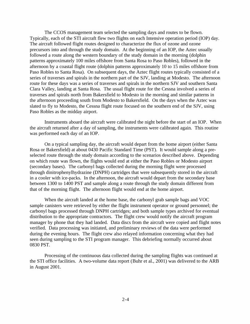
2-1. The STI Piper Aztec used during the CCOS sampling program......................................2-2
2-2. The STI Cessna and flight crew during the CCOS sampling program ............................2-3
2-3. The STI Cessna 182 used during the CCOS sampling program......................................2-3
3-1. Sensor location and sample air inlet systems on the Aztec..............................................3-4
3-2. A schematic drawing of the sample delivery systems used for ozone, CO, VOC,and carbonyl sampling .....................................................................................................3-5
3-3. An engineering design drawing of the NOy inlet system used on the STI Aztec ............3-6
3-4. Morning flight routes executed by the STI Aztec (endpoint at Santa Rosa)and Cessna (endpoint at Bakersfield) at the start of an IOP period ...............................3-24
3-5. Afternoon flight routes executed by the STI Aztec (endpoint at Santa Rosa)and Cessna (endpoint at Bakersfield) at the start of an IOP period ...............................3-25
3-6. Morning flight routes executed by the STI Aztec (endpoint at Santa Rosa)and Cessna (endpoint at Bakersfield) during an ozone episode in the SJV ...................3-26
3-7. Afternoon flight routes executed by the STI Aztec (endpoint at Santa Rosa)and Cessna (endpoint at Bakersfield) during an ozone episode in the SJV ...................3-27
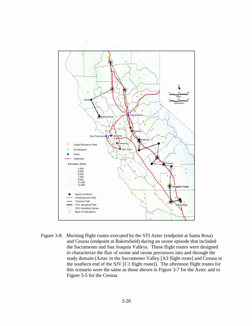
3-8. Morning flight routes executed by the STI Aztec (endpoint at Santa Rosa)and Cessna (endpoint at Bakersfield) during an ozone episode that included theSacramento and San Joaquin Valleys.............................................................................3-28
4-1. An example flight summary sheet for the Aztec flight conducted on the morningof July 23, 2000................................................................................................................4-4
4-2. An example flight map for the Aztec flight conducted on the morning ofJuly 30, 2000 ....................................................................................................................4-5
4-3. An example vertical profile from data collected during the July 30, 2000,morning Aztec flight ........................................................................................................4-6
4-4. An example traverse data plot from the data collected during the July 30, 2000,morning Aztec flight ........................................................................................................4-7
x
LIST OF FIGURES (Concluded)
Figure Page
5-1. Time series of the ozone data collected aboard the STI Aztec and the STICessna 182 during the July 6, 2000, intercomparison flight ..........................................5-10
5-2. Time series of the NO data collected aboard the STI Aztec and the STICessna 182 during the July 6, 2000, intercomparison flight ..........................................5-11
5-3. Time series of the NOy data collected aboard the STI Aztec and the STICessna 182 during the July 6, 2000, intercomparison flight ..........................................5-11
xi
LIST OF TABLES
Table Page
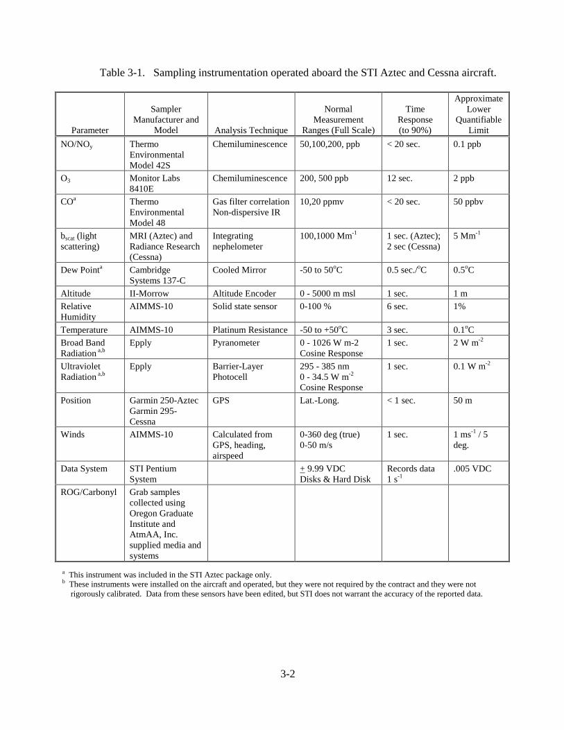
3-1. Sampling instrumentation operated aboard the STI Aztec and Cessna aircraft ...............3-2
3-2. Summary of STI Aztec sampling flights during CCOS.................................................3-11
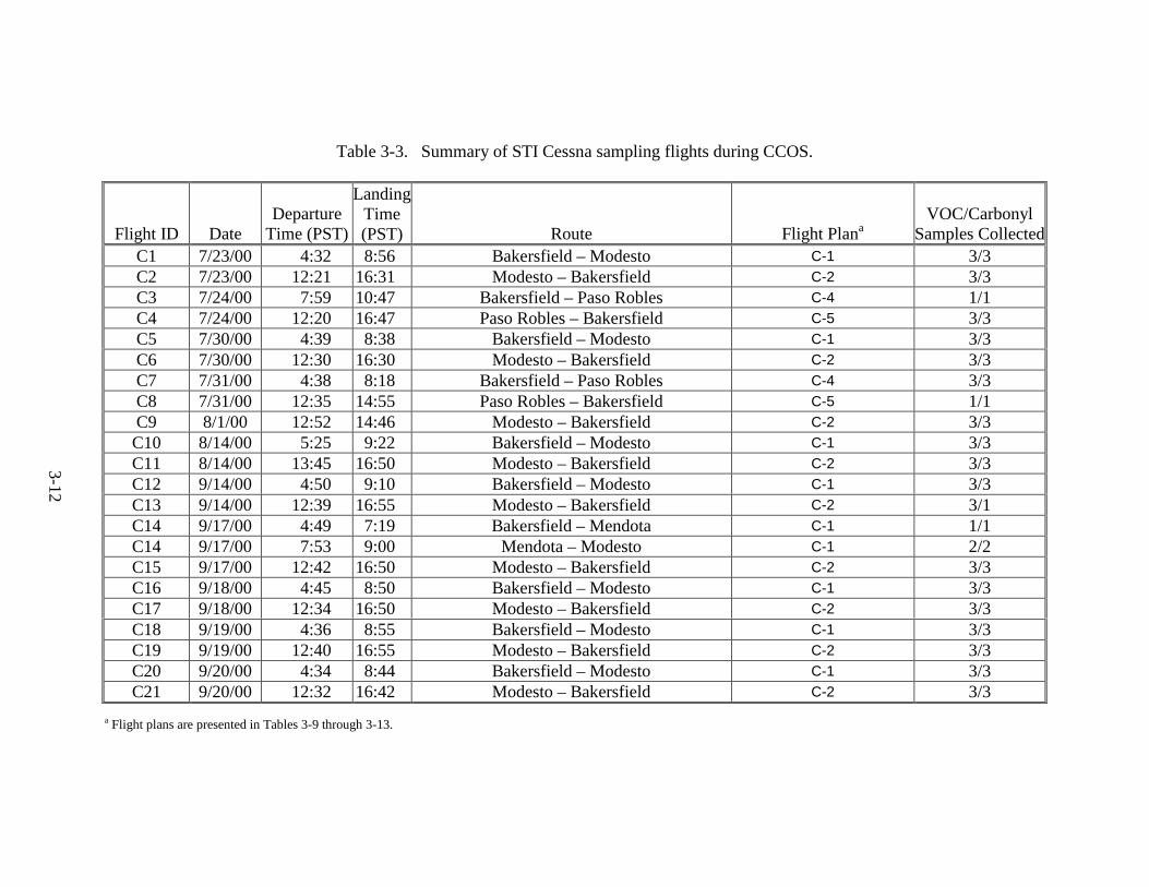
3-3. Summary of STI Cessna sampling flights during CCOS...............................................3-12
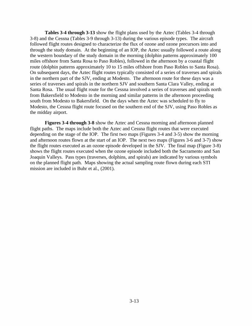
3-4. Flight plan A-1: Aztec Coastal Flight Plan, Santa Rosa to Paso Robles ......................3-14
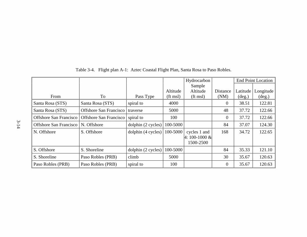
3-5. Flight plan A-2: Aztec Coastal Flight Plan, Paso Robles to Santa Rosa ......................3-15
3-6. Flight plan A-3: Aztec Northern Boundary Flight Plan, Santa Rosa to Modesto.........3-16
3-7. Flight plan A-4: Aztec Northern San Joaquin Valley Flight Plan, Santa Rosa toModesto..........................................................................................................................3-17
3-8. Flight plan A-5: Aztec Northern San Joaquin Valley Flight Plan, Modesto toSanta Rosa ......................................................................................................................3-18
3-9. Flight plan C-1: Cessna San Joaquin Valley Flight Plan, Bakersfield to Modesto.......3-19
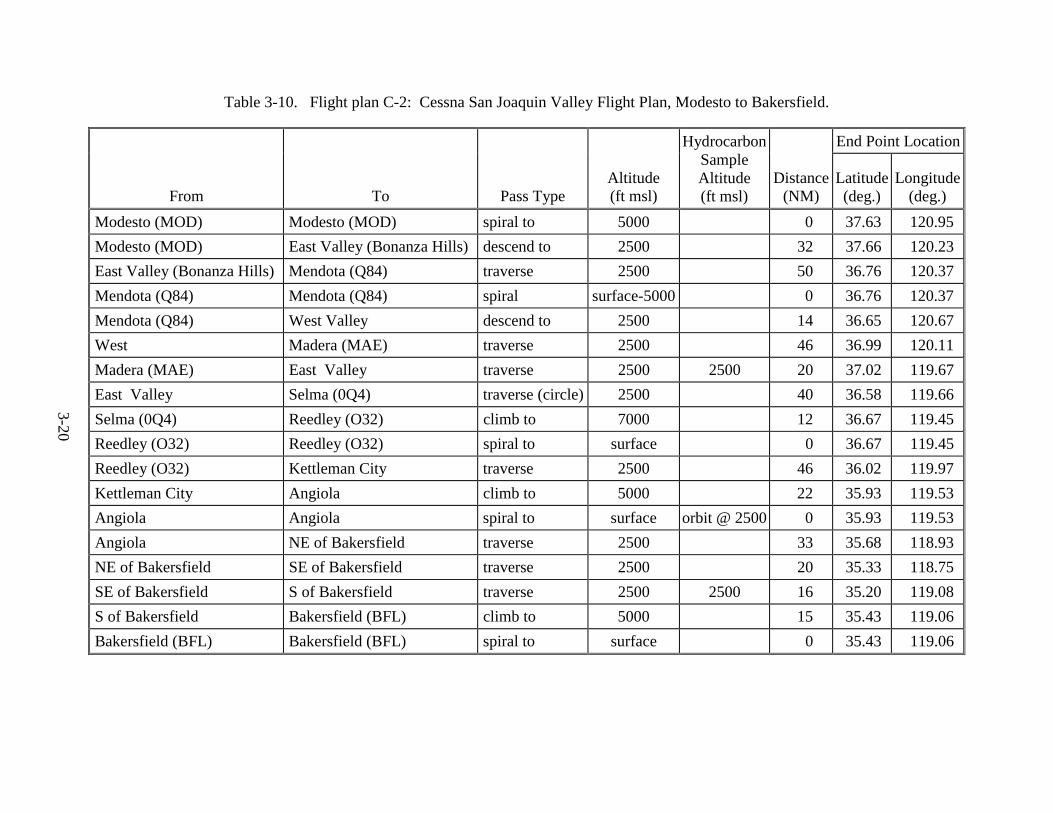
3-10. Flight plan C-2: Cessna San Joaquin Valley Flight Plan, Modesto to Bakersfield.......3-20
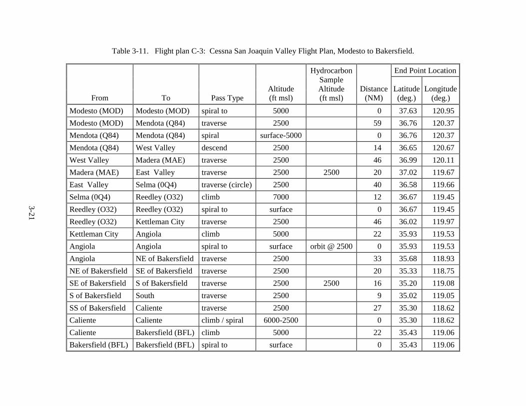
3-11. Flight plan C-3: Cessna San Joaquin Valley Flight Plan, Modesto to Bakersfield.......3-21
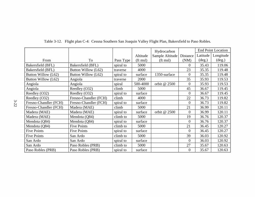
3-12. Flight plan C-4: Cessna Southern San Joaquin Valley Flight Plan, Bakersfieldto Paso Robles ................................................................................................................3-22
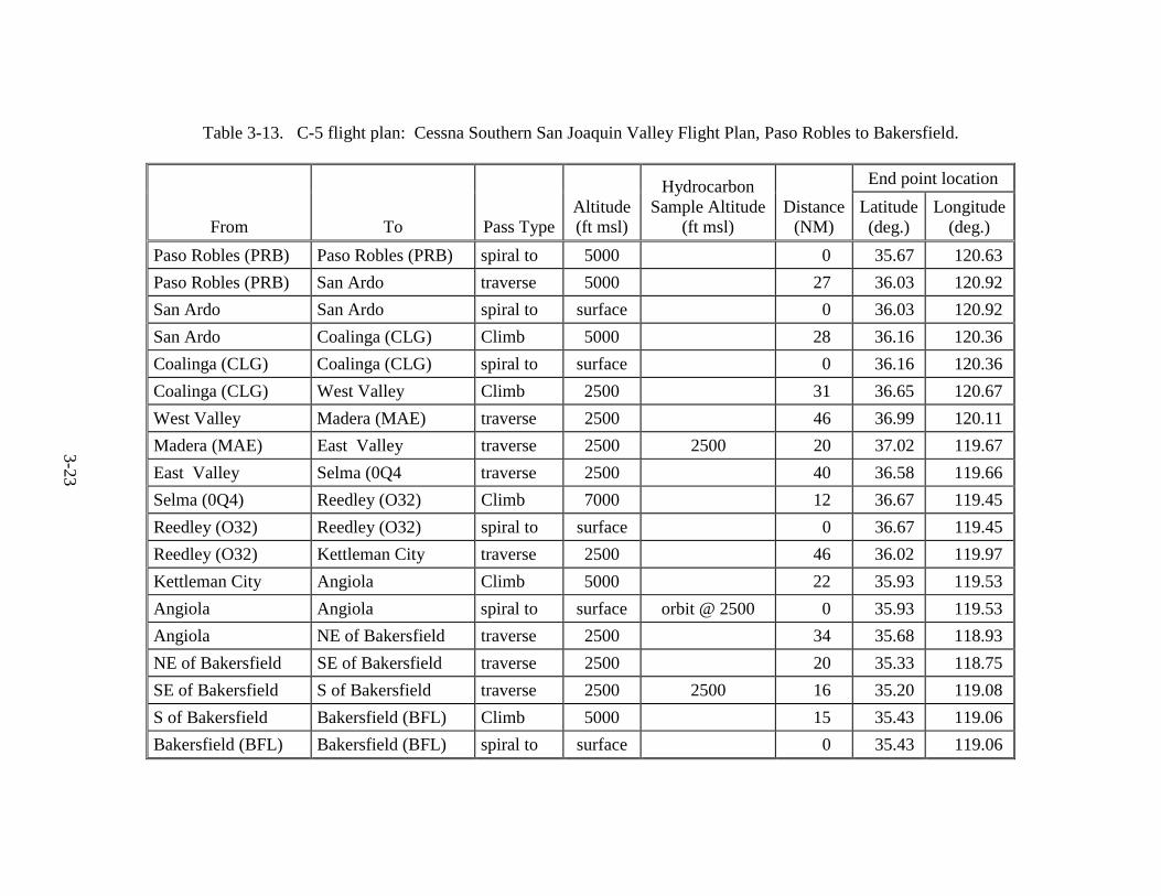
3-13. C-5 flight plan: Cessna Southern San Joaquin Valley Flight Plan, PasoRobles to Bakersfield .....................................................................................................3-23
4-1. Quality control code key. .................................................................................................4-8
5-1. Calibrations performed on the Aztec instrument suite during the CCOSoperational period.............................................................................................................5-3
5-2. Calibrations performed on the Cessna 182 instrument suite during the CCOSoperational period.............................................................................................................5-5
5-3. Preliminary audit results reported by the ARB for instrumentation auditedaboard the STI Aztec during the July 3, 2000, performance audit...................................5-8
5-4. Preliminary audit results reported by the ARB for instrumentation auditedaboard the STI Cessna during the July 3, 2000, performance audit.................................5-8
ES-1
EXECUTIVE SUMMARY
ES.1 BACKGROUND
From July through mid-September, 2000, the Central California Ozone Study (CCOS)was conducted to provide information on boundary conditions and the three-dimensionaldistribution of ozone and its precursors in the San Joaquin Valley (SJV). Sonoma Technology,Inc. (STI) was selected by the California Air Resources Board (ARB) to perform measurementsof aloft air quality and meteorology over water on the western boundary of the study domain, inthe SJV, and on one occasion in the Sacramento Valley. Two instrumented aircraft were flownby STI: a Piper Aztec based in Santa Rosa, California, and a Cessna 182 based in Bakersfield,California. Data collected during airborne sampling by both aircraft will provide information onboundary conditions and the three-dimensional distribution of ozone and its precursors in thestudy domain. The data will be used for (1) model input and evaluation, (2) documenting aloftlayers and estimating their effects on surface concentrations, and (3) improving currentunderstanding of tropospheric ozone formation and transport mechanisms within the studydomain.
CCOS was sponsored by the San Joaquin Valleywide Air Pollution Study Agency and ispart of the Central California Air Quality Studies (CCAQS). CCOS contracts were administeredby the ARB.
ES.2 METHODOLOGY
A total of 38 sampling missions (flights) were performed on 15 days between July 5 andSeptember 20, 2000, between the two aircraft. Continuous measurements made by samplingsystems on both aircraft included ozone, oxides of nitrogen (NO and NOy), light scattering (bscatusing integrating nephelometry), temperature, relative humidity, altitude, and position. Separatesampling systems were used to collect integrated grab samples for subsequent hydrocarbon andcarbonyl analysis. In addition, continuous measurements of carbon monoxide (CO)concentration were made on Aztec. The NO/NOy, ozone, and CO monitors were audited by theQuality Assurance Section of the ARB. Other quality control (QC) activities included extensivecalibrations between flight days and intercomparisons with other aircraft and with surfacemonitoring stations.
The ARB CCOS management team selected the sampling days and routes to be flown.Typically, each of the aircraft flew two flights on each Intensive Operation Period (IOP) day.The aircraft followed flight routes designed to characterize the flux of ozone and ozoneprecursors into and through the study domain. At the beginning of an IOP, the Aztec usuallyfollowed a route along the Western Boundary of the study domain in the morning (dolphinpatterns approximately 100 miles offshore from Santa Rosa to Paso Robles), followed in theafternoon by a coastal flight route (dolphin patterns approximately 10 to 15 miles offshore fromPaso Robles to Santa Rosa). On subsequent days, the Aztec flight routes typically consisted of aseries of traverses and spirals in the northern part of the SJV from Santa Rosa to Modesto. Theafternoon route for these days was a series of traverses and spirals between Modesto and Santa
ES-2
Rosa. The usual flight route for the Cessna involved a series of traverses and spirals north fromBakersfield to Modesto in the morning and similar patterns in the afternoon proceeding southfrom Modesto to Bakersfield. On the days when the Aztec was scheduled to fly to Modesto, theCessna flight route focused on the southern end of the SJV, using Paso Robles as the middayairport.
ES.3 RESULTS AND RECOMMENDATIONS
The air composition and meteorology observations made with the STI aircraft duringCCOS comprise a useful database for further exploration of transport and chemical processes inthe SJV and upwind regions. The greatest utility of the Aztec data may be in establishing limitson the upwind boundary conditions. The observations made with the Cessna will be useful inexploration of the transport processes and chemical evolution attendant to ozone episodes in theSJV.
Highlights of the observations made with the Aztec include
• High quality data for ozone, NO, NOy, CO, bscat, and winds collected offshore at altitudesfrom 500-5000 ft. under a variety of conditions.
• Persistent layers of ozone concentration greater than 50 ppbv in air masses coming fromthe Pacific Ocean.
• Significant transport of pollutants from onshore sources to points 100 miles offshore.Preliminary evaluation of the air composition in these polluted layers suggest a forest firesource.
Highlights of the observations made with the Cessna include
• Excellent temporal and spatial coverage of the southern SJV during the two principalozone episodes experienced during summer 2000.
• Good spatial and chemical characterization of the Fresno and Bakersfield urban plumesand their transport to the greater valley.
• Multi-day repetitive flight patterns that will allow exploration of the physical andchemical conditions associated with SJV-wide ozone episodes.
In addition to providing a database useful for model evaluation, these observations couldbe used to investigate a number of specific topics:
• Compare and contrast ozone distribution and ozone production efficiency at the surfaceand aloft for the Bakersfield, Fresno, and Angiola field sites.
• Examine rural ozone in the SJV with respect to sources of precursors, dynamics, andlocal production versus advection
• Contribution of forest fires to SJV ozone and particulate matter.
1-1
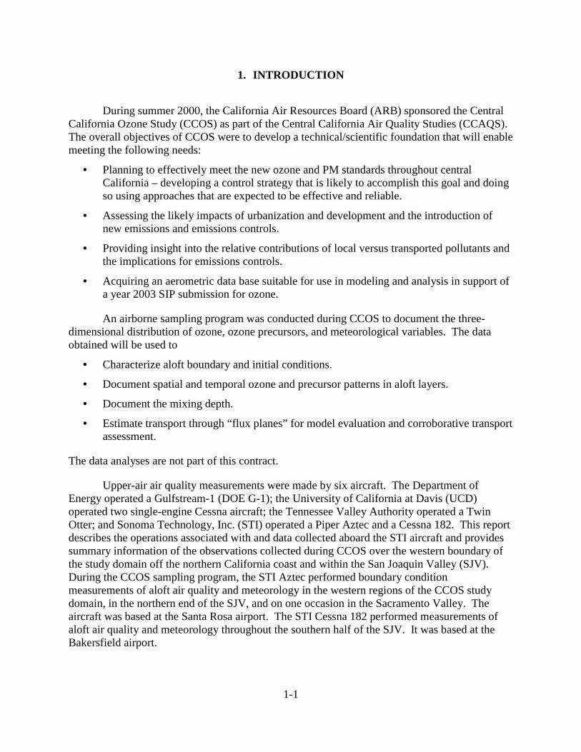
1. INTRODUCTION
During summer 2000, the California Air Resources Board (ARB) sponsored the CentralCalifornia Ozone Study (CCOS) as part of the Central California Air Quality Studies (CCAQS).The overall objectives of CCOS were to develop a technical/scientific foundation that will enablemeeting the following needs:
• Planning to effectively meet the new ozone and PM standards throughout centralCalifornia – developing a control strategy that is likely to accomplish this goal and doingso using approaches that are expected to be effective and reliable.
• Assessing the likely impacts of urbanization and development and the introduction ofnew emissions and emissions controls.
• Providing insight into the relative contributions of local versus transported pollutants andthe implications for emissions controls.
• Acquiring an aerometric data base suitable for use in modeling and analysis in support ofa year 2003 SIP submission for ozone.
An airborne sampling program was conducted during CCOS to document the three-dimensional distribution of ozone, ozone precursors, and meteorological variables. The dataobtained will be used to
• Characterize aloft boundary and initial conditions.
• Document spatial and temporal ozone and precursor patterns in aloft layers.
• Document the mixing depth.
• Estimate transport through “flux planes” for model evaluation and corroborative transportassessment.
The data analyses are not part of this contract.
Upper-air air quality measurements were made by six aircraft. The Department ofEnergy operated a Gulfstream-1 (DOE G-1); the University of California at Davis (UCD)operated two single-engine Cessna aircraft; the Tennessee Valley Authority operated a TwinOtter; and Sonoma Technology, Inc. (STI) operated a Piper Aztec and a Cessna 182. This reportdescribes the operations associated with and data collected aboard the STI aircraft and providessummary information of the observations collected during CCOS over the western boundary ofthe study domain off the northern California coast and within the San Joaquin Valley (SJV).During the CCOS sampling program, the STI Aztec performed boundary conditionmeasurements of aloft air quality and meteorology in the western regions of the CCOS studydomain, in the northern end of the SJV, and on one occasion in the Sacramento Valley. Theaircraft was based at the Santa Rosa airport. The STI Cessna 182 performed measurements ofaloft air quality and meteorology throughout the southern half of the SJV. It was based at theBakersfield airport.
1-2
Continuous measurement data collected during STI sampling flights were processed,edited, and reported to the ARB in a two-volume data report entitled “Central California OzoneStudy Aircraft Data” (Buhr et al., 2001). The data report details the sampling that wasperformed and displays plots of the data collected by the continuous sensors aboard the twoaircraft. Electronic copies of the final processed data set were also delivered to the ARB as partof the data report.
Integrated grab samples for volatile organic compounds (VOCs) and carbonyl analyseswere collected during most flights. Details of the collection of these samples were included inthe data report. The grab samples were delivered to other contractors who were responsible foranalyzing the samples and reporting the analytical results.
2-1
2. OVERVIEW OF THE STI AIRBORNE SAMPLING PROGRAM
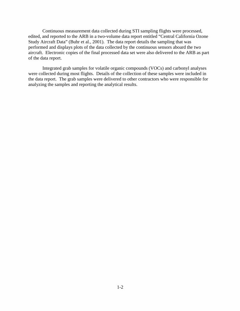
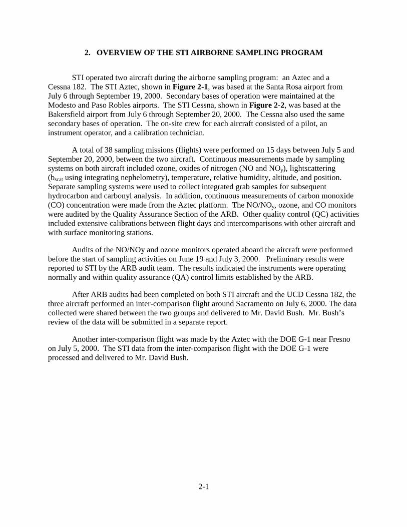
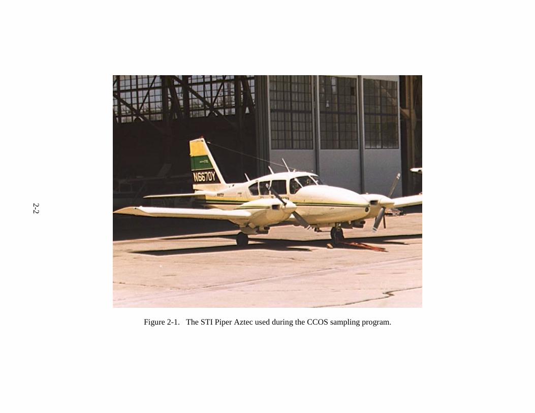
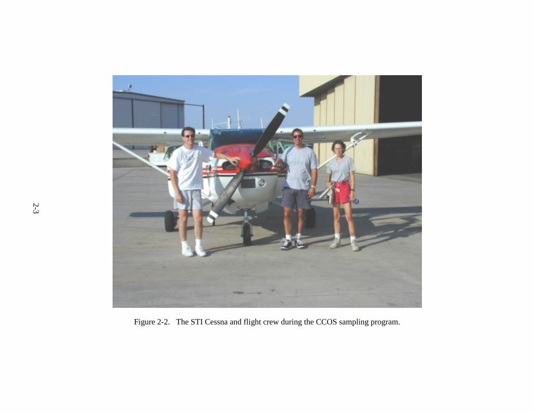
STI operated two aircraft during the airborne sampling program: an Aztec and aCessna 182. The STI Aztec, shown in Figure 2-1, was based at the Santa Rosa airport fromJuly 6 through September 19, 2000. Secondary bases of operation were maintained at theModesto and Paso Robles airports. The STI Cessna, shown in Figure 2-2, was based at theBakersfield airport from July 6 through September 20, 2000. The Cessna also used the samesecondary bases of operation. The on-site crew for each aircraft consisted of a pilot, aninstrument operator, and a calibration technician.
A total of 38 sampling missions (flights) were performed on 15 days between July 5 andSeptember 20, 2000, between the two aircraft. Continuous measurements made by samplingsystems on both aircraft included ozone, oxides of nitrogen (NO and NOy), lightscattering(bscat using integrating nephelometry), temperature, relative humidity, altitude, and position.Separate sampling systems were used to collect integrated grab samples for subsequenthydrocarbon and carbonyl analysis. In addition, continuous measurements of carbon monoxide(CO) concentration were made from the Aztec platform. The NO/NOy, ozone, and CO monitorswere audited by the Quality Assurance Section of the ARB. Other quality control (QC) activitiesincluded extensive calibrations between flight days and intercomparisons with other aircraft andwith surface monitoring stations.
Audits of the NO/NOy and ozone monitors operated aboard the aircraft were performedbefore the start of sampling activities on June 19 and July 3, 2000. Preliminary results werereported to STI by the ARB audit team. The results indicated the instruments were operatingnormally and within quality assurance (QA) control limits established by the ARB.
After ARB audits had been completed on both STI aircraft and the UCD Cessna 182, thethree aircraft performed an inter-comparison flight around Sacramento on July 6, 2000. The datacollected were shared between the two groups and delivered to Mr. David Bush. Mr. Bush’sreview of the data will be submitted in a separate report.
Another inter-comparison flight was made by the Aztec with the DOE G-1 near Fresnoon July 5, 2000. The STI data from the inter-comparison flight with the DOE G-1 wereprocessed and delivered to Mr. David Bush.
2-2
Figure 2-1. The STI Piper Aztec used during the CCOS sampling program.
2-3
Figure 2-2. The STI Cessna and flight crew during the CCOS sampling program.
2-4
The CCOS management team selected the sampling days and routes to be flown.Typically, each of the STI aircraft flew two flights on each Intensive operation period (IOP) day.The aircraft followed flight routes designed to characterize the flux of ozone and ozoneprecursors into and through the study domain. At the beginning of an IOP, the Aztec usuallyfollowed a route along the western boundary of the study domain in the morning (dolphinpatterns approximately 100 miles offshore from Santa Rosa to Paso Robles), followed in theafternoon by a coastal flight route (dolphin patterns approximately 10 to 15 miles offshore fromPaso Robles to Santa Rosa). On subsequent days, the Aztec flight routes typically consisted of aseries of traverses and spirals in the northern part of the SJV, landing at Modesto. The afternoonroute for these days was a series of traverses and spirals in the northern SJV and southern SantaClara Valley, landing at Santa Rosa. The usual flight route for the Cessna involved a series oftraverses and spirals north from Bakersfield to Modesto in the morning and similar patterns inthe afternoon proceeding south from Modesto to Bakersfield. On the days when the Aztec wasslated to fly to Modesto, the Cessna flight route focused on the southern end of the SJV, usingPaso Robles as the midday airport.
Instruments aboard the aircraft were calibrated the night before the start of an IOP. Whenthe aircraft returned after a day of sampling, the instruments were calibrated again. This routinewas performed each day of an IOP.
On a typical sampling day, the aircraft would depart from the home airport (either SantaRosa or Bakersfield) at about 0430 Pacific Standard Time (PST). It would sample along a pre-selected route through the study domain according to the scenarios described above. Dependingon which route was flown, the flights would end at either the Paso Robles or Modesto airport(secondary bases). The carbonyl bags collected during the morning flight were processedthrough dinitrophenylhydrazine (DNPH) cartridges that were subsequently stored in the aircraftin a cooler with ice-packs. In the afternoon, the aircraft would depart from the secondary basebetween 1300 to 1400 PST and sample along a route through the study domain different fromthat of the morning flight. The afternoon flight would end at the home airport.
When the aircraft landed at the home base, the carbonyl grab sample bags and VOCsample canisters were retrieved by either the flight instrument operator or ground personnel; thecarbonyl bags processed through DNPH cartridges; and both sample types archived for eventualdistribution to the appropriate contractors. The flight crew would notify the aircraft programmanager by phone that they had landed. Data discs from the aircraft were copied and flight notesverified. Data processing was initiated, and preliminary reviews of the data were performedduring the evening hours. The flight crew also relayed information concerning what they hadseen during sampling to the STI program manager. This debriefing normally occurred about0830 PST.
Processing of the continuous data collected during the sampling flights was continued atthe STI office facilities. A two-volume data report (Buhr et al., 2001) was delivered to the ARBin August 2001.
3-1
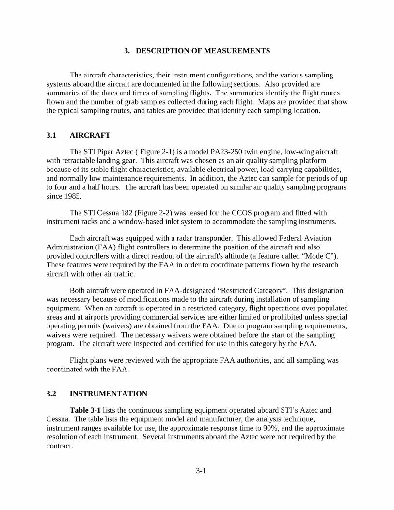
3. DESCRIPTION OF MEASUREMENTS
The aircraft characteristics, their instrument configurations, and the various samplingsystems aboard the aircraft are documented in the following sections. Also provided aresummaries of the dates and times of sampling flights. The summaries identify the flight routesflown and the number of grab samples collected during each flight. Maps are provided that showthe typical sampling routes, and tables are provided that identify each sampling location.
3.1 AIRCRAFT
The STI Piper Aztec ( Figure 2-1) is a model PA23-250 twin engine, low-wing aircraftwith retractable landing gear. This aircraft was chosen as an air quality sampling platformbecause of its stable flight characteristics, available electrical power, load-carrying capabilities,and normally low maintenance requirements. In addition, the Aztec can sample for periods of upto four and a half hours. The aircraft has been operated on similar air quality sampling programssince 1985.
The STI Cessna 182 (Figure 2-2) was leased for the CCOS program and fitted withinstrument racks and a window-based inlet system to accommodate the sampling instruments.
Each aircraft was equipped with a radar transponder. This allowed Federal AviationAdministration (FAA) flight controllers to determine the position of the aircraft and alsoprovided controllers with a direct readout of the aircraft's altitude (a feature called “Mode C”).These features were required by the FAA in order to coordinate patterns flown by the researchaircraft with other air traffic.
Both aircraft were operated in FAA-designated “Restricted Category”. This designationwas necessary because of modifications made to the aircraft during installation of samplingequipment. When an aircraft is operated in a restricted category, flight operations over populatedareas and at airports providing commercial services are either limited or prohibited unless specialoperating permits (waivers) are obtained from the FAA. Due to program sampling requirements,waivers were required. The necessary waivers were obtained before the start of the samplingprogram. The aircraft were inspected and certified for use in this category by the FAA.
Flight plans were reviewed with the appropriate FAA authorities, and all sampling wascoordinated with the FAA.
3.2 INSTRUMENTATION
Table 3-1 lists the continuous sampling equipment operated aboard STI’s Aztec andCessna. The table lists the equipment model and manufacturer, the analysis technique,instrument ranges available for use, the approximate response time to 90%, and the approximateresolution of each instrument. Several instruments aboard the Aztec were not required by thecontract.
3-2
Table 3-1. Sampling instrumentation operated aboard the STI Aztec and Cessna aircraft.
Parameter
SamplerManufacturer and
Model Analysis Technique
NormalMeasurement
Ranges (Full Scale)
TimeResponse(to 90%)
ApproximateLower
QuantifiableLimit
NO/NOy ThermoEnvironmentalModel 42S
Chemiluminescence 50,100,200, ppb < 20 sec. 0.1 ppb
O3 Monitor Labs8410E
Chemiluminescence 200, 500 ppb 12 sec. 2 ppb
COa ThermoEnvironmentalModel 48
Gas filter correlationNon-dispersive IR
10,20 ppmv < 20 sec. 50 ppbv
bscat (lightscattering)
MRI (Aztec) andRadiance Research(Cessna)
Integratingnephelometer
100,1000 Mm-1 1 sec. (Aztec);2 sec (Cessna)
5 Mm-1
Dew Pointa CambridgeSystems 137-C
Cooled Mirror -50 to 50oC 0.5 sec./oC 0.5oC
Altitude II-Morrow Altitude Encoder 0 - 5000 m msl 1 sec. 1 mRelativeHumidity
AIMMS-10 Solid state sensor 0-100 % 6 sec. 1%
Temperature AIMMS-10 Platinum Resistance -50 to +50oC 3 sec. 0.1oCBroad BandRadiation a,b
Epply Pyranometer 0 - 1026 W m-2Cosine Response
1 sec. 2 W m-2
UltravioletRadiation a,b
Epply Barrier-LayerPhotocell
295 - 385 nm0 - 34.5 W m-2
Cosine Response
1 sec. 0.1 W m-2
Position Garmin 250-AztecGarmin 295-Cessna
GPS Lat.-Long. < 1 sec. 50 m
Winds AIMMS-10 Calculated fromGPS, heading,airspeed
0-360 deg (true)0-50 m/s
1 sec. 1 ms-1 / 5deg.
Data System STI PentiumSystem
+ 9.99 VDCDisks & Hard Disk
Records data1 s-1
.005 VDC
ROG/Carbonyl Grab samplescollected usingOregon GraduateInstitute andAtmAA, Inc.supplied media andsystems
a This instrument was included in the STI Aztec package only.b These instruments were installed on the aircraft and operated, but they were not required by the contract and they were not
rigorously calibrated. Data from these sensors have been edited, but STI does not warrant the accuracy of the reported data.
3-3
These instruments were operated and their data processed although they were notcalibrated. These instruments are also identified in Table 3-1. Data from these instruments wereincluded in the aircraft database, but their data should be used with caution. All requiredmeasurements were processed, quality controlled, and reported as “Level 1” quality controlleddata.
As shown in Table 3-1, grab samples to be analyzed for VOC and carbonylconcentrations were also collected aboard the aircraft. The collection media and samplingsystems were provided by Oregon Graduate Institute and AtmAA, Inc., respectively.
3.3 SAMPLING SYSTEMS
3.3.1 Access to Ambient Air
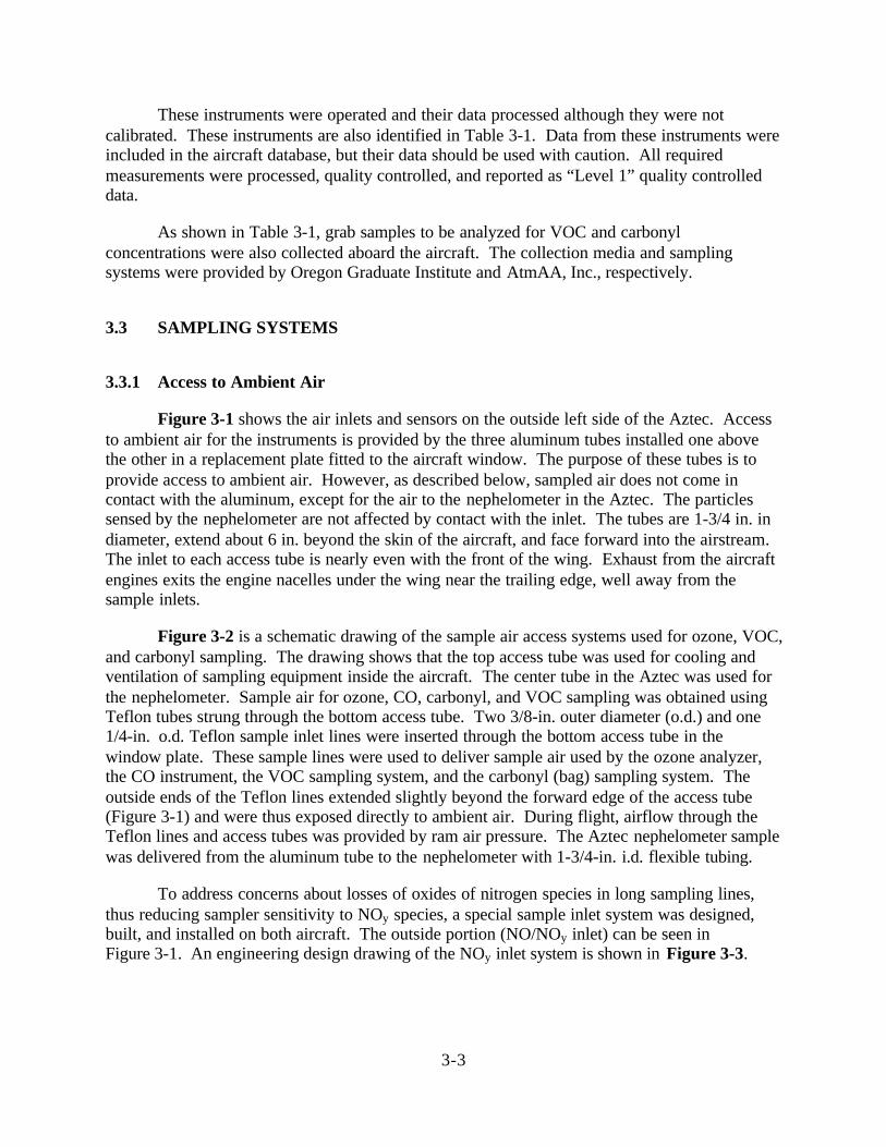
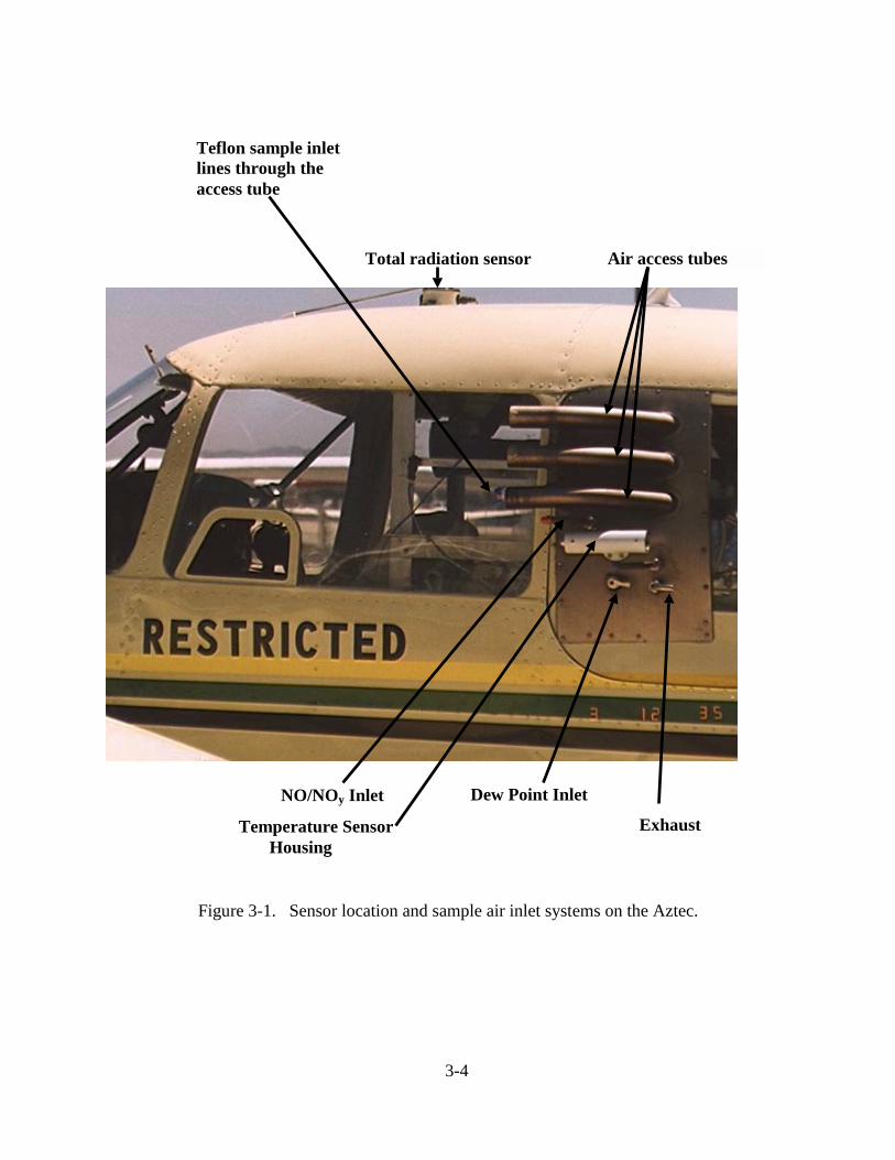
Figure 3-1 shows the air inlets and sensors on the outside left side of the Aztec. Accessto ambient air for the instruments is provided by the three aluminum tubes installed one abovethe other in a replacement plate fitted to the aircraft window. The purpose of these tubes is toprovide access to ambient air. However, as described below, sampled air does not come incontact with the aluminum, except for the air to the nephelometer in the Aztec. The particlessensed by the nephelometer are not affected by contact with the inlet. The tubes are 1-3/4 in. indiameter, extend about 6 in. beyond the skin of the aircraft, and face forward into the airstream.The inlet to each access tube is nearly even with the front of the wing. Exhaust from the aircraftengines exits the engine nacelles under the wing near the trailing edge, well away from thesample inlets.
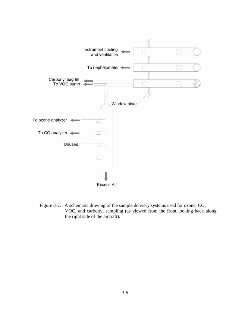
Figure 3-2 is a schematic drawing of the sample air access systems used for ozone, VOC,and carbonyl sampling. The drawing shows that the top access tube was used for cooling andventilation of sampling equipment inside the aircraft. The center tube in the Aztec was used forthe nephelometer. Sample air for ozone, CO, carbonyl, and VOC sampling was obtained usingTeflon tubes strung through the bottom access tube. Two 3/8-in. outer diameter (o.d.) and one1/4-in. o.d. Teflon sample inlet lines were inserted through the bottom access tube in thewindow plate. These sample lines were used to deliver sample air used by the ozone analyzer,the CO instrument, the VOC sampling system, and the carbonyl (bag) sampling system. Theoutside ends of the Teflon lines extended slightly beyond the forward edge of the access tube(Figure 3-1) and were thus exposed directly to ambient air. During flight, airflow through theTeflon lines and access tubes was provided by ram air pressure. The Aztec nephelometer samplewas delivered from the aluminum tube to the nephelometer with 1-3/4-in. i.d. flexible tubing.
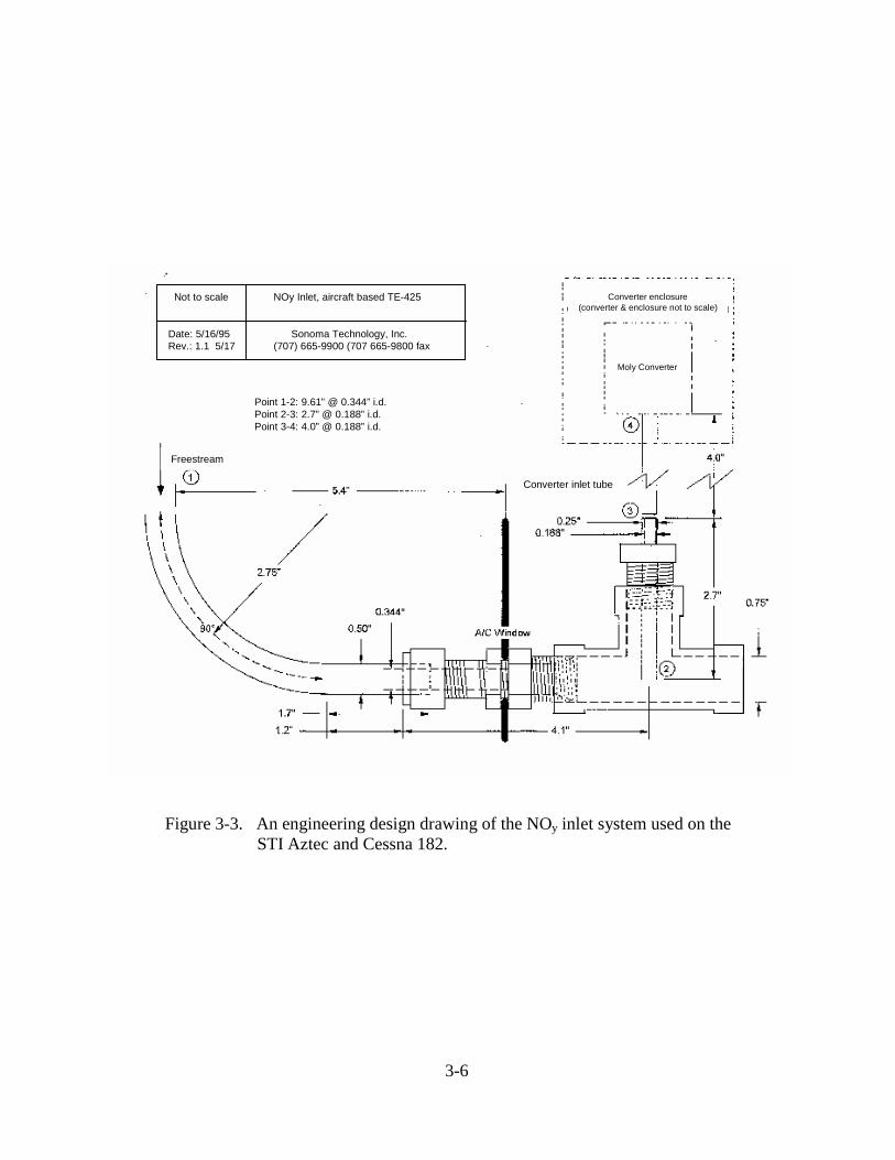
To address concerns about losses of oxides of nitrogen species in long sampling lines,thus reducing sampler sensitivity to NOy species, a special sample inlet system was designed,built, and installed on both aircraft. The outside portion (NO/NOy inlet) can be seen inFigure 3-1. An engineering design drawing of the NOy inlet system is shown in Figure 3-3.
3-4
Figure 3-1. Sensor location and sample air inlet systems on the Aztec.
Air access tubes
NO/NOy Inlet
Temperature Sensor Housing
Dew Point Inlet
Exhaust
Total radiation sensor
Teflon sample inletlines through theaccess tube
3-5
Instrument cooling and ventilation
Unused
To CO analyzer
To ozone analyzer
To VOC pumpCarbonyl bag fill
To nephelometer
Window plate
Excess Air
Figure 3-2. A schematic drawing of the sample delivery systems used for ozone, CO,VOC, and carbonyl sampling (as viewed from the front looking back alongthe right side of the aircraft).
3-6
Not to scale NOy Inlet, aircraft based TE-425
Date: 5/16/95 Sonoma Technology, Inc.Rev.: 1.1 5/17 (707) 665-9900 (707 665-9800 fax
Point 1-2: 9.61” @ 0.344” i.d.Point 2-3: 2.7” @ 0.188” i.d.Point 3-4: 4.0” @ 0.188” i.d.
Converter enclosure(converter & enclosure not to scale)
Moly Converter
Converter inlet tube
Freestream
Figure 3-3. An engineering design drawing of the NOy inlet system used on theSTI Aztec and Cessna 182.
3-7
The objective of the NOy inlet design is to prevent absorption of highly reactive speciesby the wall of the sampling inlet tube by reducing the length of the sampling line from thesample inlet to the NOy converter. This was accomplished by utilizing a modified NO/NOyanalyzer (TECO 42S after modification) with a removable NOy converter. The converter wasmounted on the inside of the window plate to bring it as near as possible to the sample inlet.Sample air was provided to the converter by means of a Teflon-coated stainless steel inlet tube, ashort Teflon-coated stainless steel manifold, and a short, heated stainless steel sample tube to theconverter itself.
Transmission of HNO3 (nitric acid) through the NOy inlet was not evaluated. However,the Teflon-coated surfaces and short residence time in the inlet are expected to lead to effectivelyquantitative transmission. The total residence time of the sample in the inlet system wasapproximately 200 msec . In addition to this short residence time, the portion of the inlet fromthe manifold (point 3 in Figure 3-3) to the converter (point 4 in Figure 3-3) was stainless steelheated by excess heat generated in the converter core and conducted throughout the length of theinlet tube. Temperatures along the converter inlet tube inside the aircraft were approximately45-60°C. The converter itself was operated at 350°C. A Teflon particle filter was placed in theNOy sample line downstream of the converter. NO was sampled from the side-port of anadditional Teflon-coated stainless steel tee attached downstream of the NOy tee (point 2 inFigure 3-3).
The inlet tube for the NOy systems was removable. Periodically, the tube was removedand cleaned.
The inlet system used on the Cessna 182 aircraft was similar in design to that describedfor the Aztec. The sample inlets were fitted through holes bored in the right side rear windowand included a NO/NOy inlet identical to the Aztec inlet and two 1-in. o.d. aluminum tubes. Oneof the aluminum tubes served as the nephelometer inlet, coupled to the nephelometer withflexible tubing, and the other aluminum tube held the 3/8-in. and 1/4-in. Teflon sample lines forthe ozone monitor, carbonyl, and VOC sample lines.
The exhaust for the Cessna 182 was pushed under the aircraft and up the left side, awayfrom the sample inlets. Sampling in clean air confirmed that there was no exhaust contaminationon the Cessna 182.
3.3.2 Sample Delivery Systems
Continuous sensors
One of the 3/8-in. inlet lines (discussed in Section 3.3.1) was used to provide sample airto a glass manifold from which the ozone (and, in the Aztec, CO) monitors sampled. Themanifold consisted of a 3/8-in. inlet into a glass expansion chamber (Figure 3-2) measuring 9 in.in length by 1 in. in diameter. Three 1/4-in. static sample ports were attached to the side of theexpansion chamber. Volume expansion inside the chamber slowed the incoming sample airflow.A Teflon sampling line from the ozone monitor was connected to the first port (nearest themanifold inlet). The second port in the Aztec was attached to the CO instrument, and the thirdport was not used. Excess air from the glass manifold was vented into the cabin of the aircraft.The ozone monitor was operated using a Teflon particle inlet filter.
3-8
Two 1/4-in. o.d. Teflon sample lines delivered sample air from the inlet system directlyto the NO/NOy analyzer. The sample lines were cut to the same length in an attempt to time-match recorded concentration values.
All connections used Teflon fittings. Thus, for the gas analyzers, an incoming air samplewas only in contact with Teflon, stainless steel, or glass, from the atmosphere to the inlet of asampling instrument.
VOC grab sampling
The VOC sampling system was provided by the Oregon Graduate Center andconsisted of
• A 2.4-m (8 ft) length of 1/4-in.-diameter Teflon sample inlet tube, • One KNF Neuberger pump (DC voltage), • A Veriflo flow regulator with a preset 25 psi back pressure, • A 1.8-m (6 ft) length of 6.5-mm Teflon sample delivery tubing, • A two-way toggle valve and pressure gauge assembly (called a "purge tee"), and • 1.5-liter stainless steel canisters.
The sampling system was configured so that the entire sample line up to the canistercould be flushed with ambient air prior to collecting a sample. To collect a sample, the purge teewas closed and the canister valve opened. Sample collection took about 30-45 seconds and wascomplete when the canister pressure was about 25 psig.
As described in Section 3.3.1 and shown in Figure 3-2, the 1/4-in. o.d.Teflon sample inlettube was inserted through the bottom access tube in the sampling window. The other end wasconnected to the VOC pumps. The pumps supplied air through the flow regulator and sampledelivery tubing to the purge tee. The position of the toggle valve on the purge tee allowedsample air to be either exhausted into the aircraft cabin or directed into the sample canister.
The flow regulator was adjusted to fully pressurize a canister in less than one minute.Since bag and VOC samples were collected together, this fill rate was selected to match the filltime for bag samples (discussed below).
During flight, the pump was run continuously to purge the sampling system. Wheneverthe aircraft was on the ground, the VOC system was sealed on both ends to avoid contamination.Essentially identical VOC sampling systems were used on both the Aztec and Cessna 182aircraft.
Carbonyl grab sampling
The system for grab bag collection was provided by AtmAA, Inc. and consisted of a1.2-m (4-ft) length of 3/8-in. o.d. Teflon tubing that was inserted through the bottom access tubeon the sampling window. The inlet tubing terminated in a two-piece reduction assemblyconsisting of 3/8-in. o.d. tubing and 1/4-in. o.d. tubing telescoped together.
The 40-liter-volume sample bags were constructed of 2-mil Tedlar material. The inleton each bag was a “Push to Open - Pull to Close” type stainless steel valve. The bag valve was
3-9
connected to the sample line by a snug friction fit between the valve and the tubing. The bagwas filled using ram air pressure. When the system was not sampling, air flow through the inlettubing provided a continual purge of the system.
After an air sample was collected aboard the aircraft and the sample bag had beendisconnected from the sampling system, the sample bag was placed inside a larger dark opaqueplastic bag. These bags were used to inhibit photochemical reactions in the sample bags untilthe contents could be collected onto DNPH cartridges post-flight. Typically, these sampletransfers were completed within about an hour of receiving the bag samples. The DNPHcartridges were stored in a cooler except during sample transfer.
Sample bags were reused after ground-based transfer operations had been completed.Conditioning of bags prior to use (or reuse) was performed by STI personnel and includedmultiple flushes of the bags with zero air, followed by injection of about 10 mL of 1000 ppmvNO in nitrogen (N2) into the deflated bag. The purpose of the NO was to provide a preferentialspecies for ambient ozone to oxidize once a sample was collected, thus minimizing oxidation ofthe target carbonyl species.
Again, the sampling system and sample handling procedures were identical for the Aztecand Cessna 182 aircraft.
3.4 SENSOR MOUNTING LOCATIONS
The sensors aboard the aircraft can be divided into two groups: external- and internal-mounted sensors.
3.4.1 External-mounted Sensors
The primary temperature probe used aboard the Aztec was mounted on the outside of thesampling window plate. The vortex housing assembly that contained the bead thermistor sensoris shown in Figure 3-1. Holes drilled through the sampling window provided electrical access tothe sensor. A secondary (back-up) temperature probe was mounted under the right wing of theaircraft.
Dew point, turbulence, ultraviolet radiation, and total radiation were also measured. Theinlet system for the dew point sensor was mounted on the outside of the sampling window(Figure 3-1), and the sensor head itself was mounted on the inside of the window. Theturbulence sensor was mounted under the left wing.
Ultraviolet and total radiation sensors were mounted on the top of the aircraft cabin.Because of their placement, data from these two sensors were subjected to antenna wireshadows, varying aircraft attitudes, and radio transmission interference. Though not part of therequired data set, these sensors were operated but they were not calibrated. Their data wereedited but STI does not warrant the accuracy of the reported data.
3-10
Both the Aztec and the Cessna 182 used an AIMMS-10 wind instrument. On the Cessna,the AIMMS-10 was mounted on the left side wing strut. On the Aztec the AIMMS-10 wasmounted underneath the right wing, outboard of the engine.
3.4.2 Internal-mounted Sensors
In the Aztec, the continuous real-time air quality sensors, data acquisition system (DAS),and associated support equipment were mounted in instrument racks installed on the left side ofthe aircraft cabin, behind the pilot. In the Cessna 182 the DAS and other ancillary equipmentwas mounted in the instrument rack on the right side of the aircraft.
For both the Aztec and Cessna 182, the primary altitude data were obtained from anencoding altimeter mounted under the aircraft's instrument panel and connected to the aircraft’sstatic pressure system. In the Aztec a secondary (back-up) measurement of altitude wasprovided by a Validyne pressure transducer mounted in the rear left of the aircraft cabin. Bothwere connected to outside static air points.
Aztec position data were obtained from a Garmin Model 250 GPS receiver mounted inthe aircraft’s instrument panel. The digital output from this unit was fed into the on-board DAS.A similar system was employed in the Cessna, using a yoke-mounted Garmin 295 GPS.
3.5 INSTRUMENT EXHAUST SYSTEM
Although the exhaust system of typical air quality instruments contains some provisionfor scrubbing exhaust gases, airborne safety and the integrity of the sampling being performedrequires additional safeguards. For example, the ozone monitor used aboard the aircraft requireda steady supply of ethylene (C2H4). It is possible that some excess C2H4 could have remained inthe instrument’s exhaust, which could have interfered with VOC measurements if the exhaustwas not properly vented. To avoid potential problems, the exhaust streams from all analyzerswere combined using an exhaust manifold that vented outside the aircraft. The exhaust tube(external portion of the system) can be see in Figure 3-1. Instrument exhaust gases were pumpedout of the cabin and exhausted well aft of sensor inlet systems.
3.6 SUMMARY OF FLIGHTS, TIMES, AND ROUTES
The CCOS management team selected the sampling days and routes to be flown.Typically both the Aztec and Cessna flew two flights on each selected day. Between the twoaircraft, a total of 38 sampling missions (flights) were performed on 15 days between July 5 andSeptember 20, 2000. .
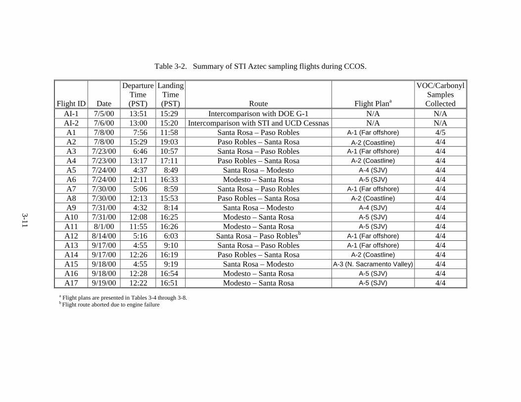
Tables 3-2 and 3-3 summarize the date, sampling period, flight route, and number ofVOC and carbonyl samples collected during each CCOS flight for the Aztec and Cessna 182,respectively. Each flight was assigned an identifying name that is also shown in the table.Details of each flight are presented in the two-volume data report that was delivered to the ARB.
3-11
Table 3-2. Summary of STI Aztec sampling flights during CCOS.
Flight ID Date
DepartureTime(PST)
LandingTime(PST) Route Flight Plana
VOC/CarbonylSamplesCollected
AI-1 7/5/00 13:51 15:29 Intercomparison with DOE G-1 N/A N/AAI-2 7/6/00 13:00 15:20 Intercomparison with STI and UCD Cessnas N/A N/AA1 7/8/00 7:56 11:58 Santa Rosa – Paso Robles A-1 (Far offshore) 4/5A2 7/8/00 15:29 19:03 Paso Robles – Santa Rosa A-2 (Coastline) 4/4A3 7/23/00 6:46 10:57 Santa Rosa – Paso Robles A-1 (Far offshore) 4/4A4 7/23/00 13:17 17:11 Paso Robles – Santa Rosa A-2 (Coastline) 4/4A5 7/24/00 4:37 8:49 Santa Rosa – Modesto A-4 (SJV) 4/4A6 7/24/00 12:11 16:33 Modesto – Santa Rosa A-5 (SJV) 4/4A7 7/30/00 5:06 8:59 Santa Rosa – Paso Robles A-1 (Far offshore) 4/4A8 7/30/00 12:13 15:53 Paso Robles – Santa Rosa A-2 (Coastline) 4/4A9 7/31/00 4:32 8:14 Santa Rosa – Modesto A-4 (SJV) 4/4A10 7/31/00 12:08 16:25 Modesto – Santa Rosa A-5 (SJV) 4/4A11 8/1/00 11:55 16:26 Modesto – Santa Rosa A-5 (SJV) 4/4A12 8/14/00 5:16 6:03 Santa Rosa – Paso Roblesb A-1 (Far offshore) 4/4A13 9/17/00 4:55 9:10 Santa Rosa – Paso Robles A-1 (Far offshore) 4/4A14 9/17/00 12:26 16:19 Paso Robles – Santa Rosa A-2 (Coastline) 4/4A15 9/18/00 4:55 9:19 Santa Rosa – Modesto A-3 (N. Sacramento Valley) 4/4A16 9/18/00 12:28 16:54 Modesto – Santa Rosa A-5 (SJV) 4/4A17 9/19/00 12:22 16:51 Modesto – Santa Rosa A-5 (SJV) 4/4
a Flight plans are presented in Tables 3-4 through 3-8.b Flight route aborted due to engine failure
3-12
Table 3-3. Summary of STI Cessna sampling flights during CCOS.
Flight ID DateDeparture
Time (PST)
LandingTime(PST) Route Flight Plana
VOC/CarbonylSamples Collected
C1 7/23/00 4:32 8:56 Bakersfield – Modesto C-1 3/3C2 7/23/00 12:21 16:31 Modesto – Bakersfield C-2 3/3C3 7/24/00 7:59 10:47 Bakersfield – Paso Robles C-4 1/1C4 7/24/00 12:20 16:47 Paso Robles – Bakersfield C-5 3/3C5 7/30/00 4:39 8:38 Bakersfield – Modesto C-1 3/3C6 7/30/00 12:30 16:30 Modesto – Bakersfield C-2 3/3C7 7/31/00 4:38 8:18 Bakersfield – Paso Robles C-4 3/3C8 7/31/00 12:35 14:55 Paso Robles – Bakersfield C-5 1/1C9 8/1/00 12:52 14:46 Modesto – Bakersfield C-2 3/3C10 8/14/00 5:25 9:22 Bakersfield – Modesto C-1 3/3C11 8/14/00 13:45 16:50 Modesto – Bakersfield C-2 3/3C12 9/14/00 4:50 9:10 Bakersfield – Modesto C-1 3/3C13 9/14/00 12:39 16:55 Modesto – Bakersfield C-2 3/1C14 9/17/00 4:49 7:19 Bakersfield – Mendota C-1 1/1C14 9/17/00 7:53 9:00 Mendota – Modesto C-1 2/2C15 9/17/00 12:42 16:50 Modesto – Bakersfield C-2 3/3C16 9/18/00 4:45 8:50 Bakersfield – Modesto C-1 3/3C17 9/18/00 12:34 16:50 Modesto – Bakersfield C-2 3/3C18 9/19/00 4:36 8:55 Bakersfield – Modesto C-1 3/3C19 9/19/00 12:40 16:55 Modesto – Bakersfield C-2 3/3C20 9/20/00 4:34 8:44 Bakersfield – Modesto C-1 3/3C21 9/20/00 12:32 16:42 Modesto – Bakersfield C-2 3/3
a Flight plans are presented in Tables 3-9 through 3-13.
3-13
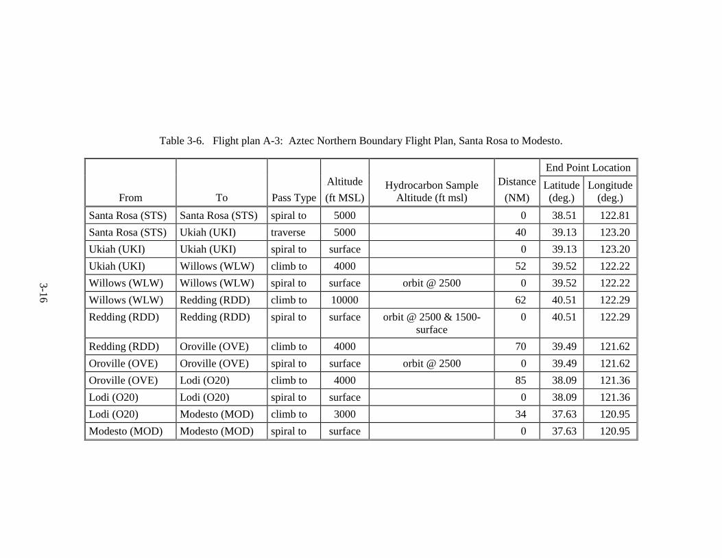
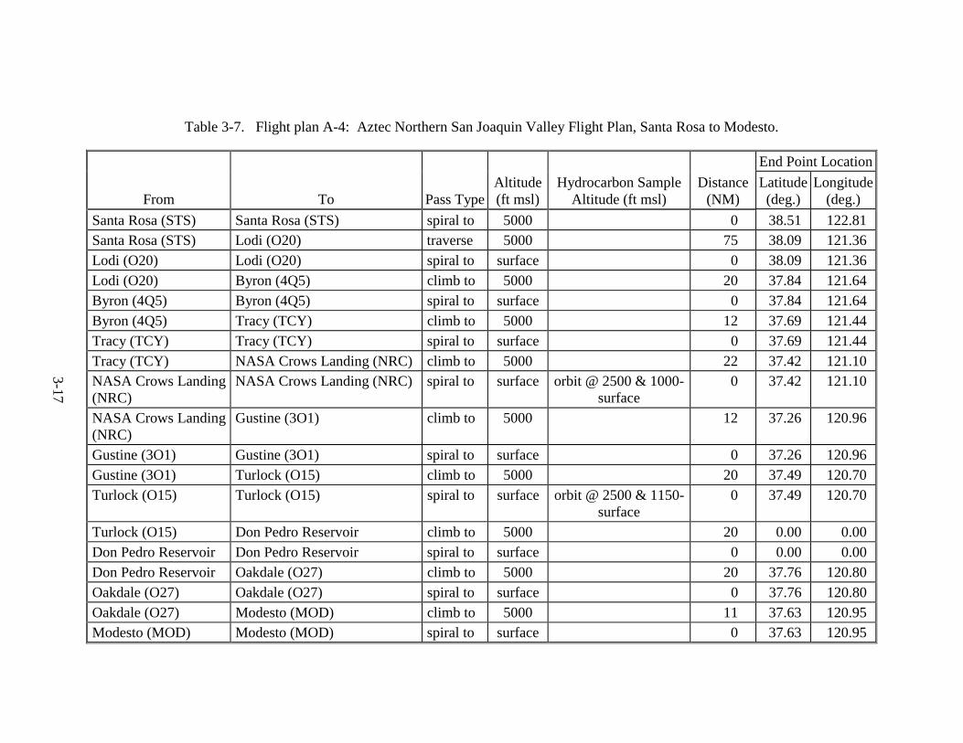
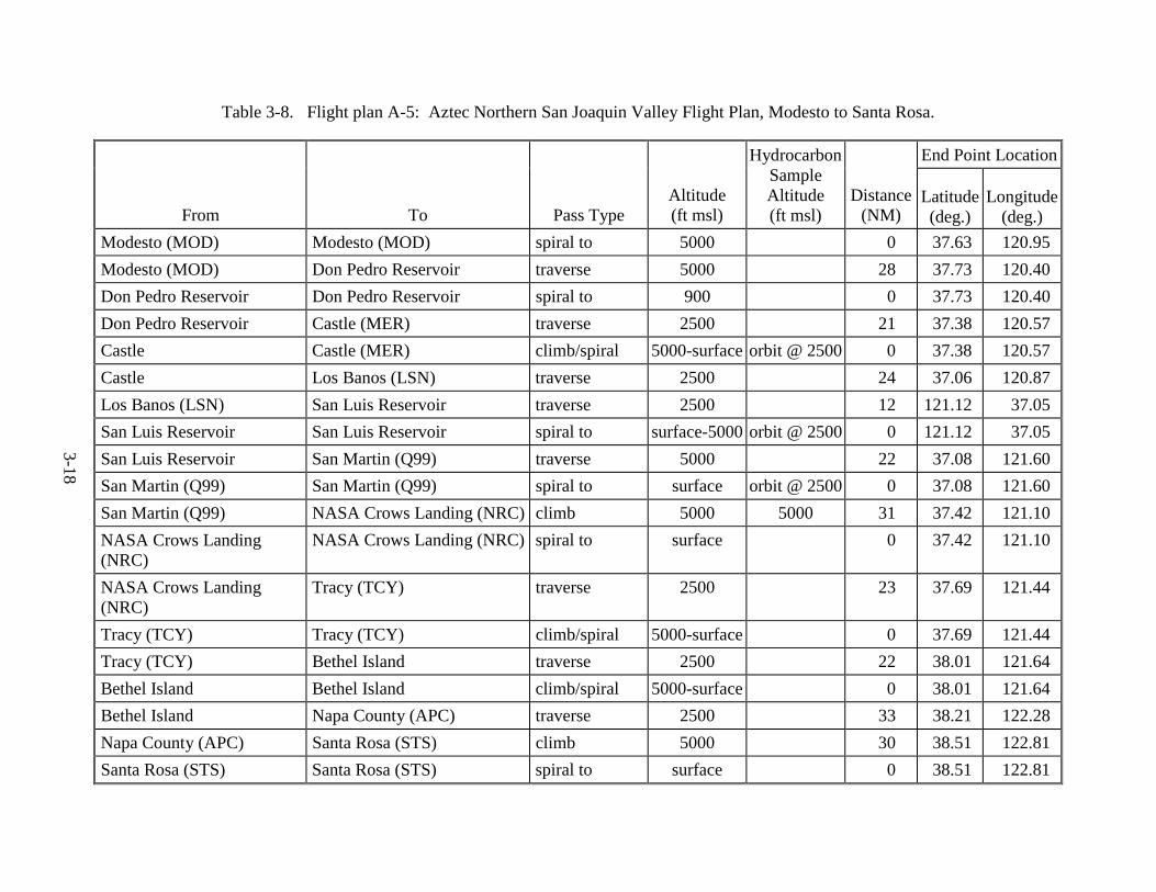
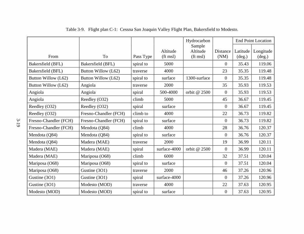
Tables 3-4 through 3-13 show the flight plans used by the Aztec (Tables 3-4 through3-8) and the Cessna (Tables 3-9 through 3-13) during the various episode types. The aircraftfollowed flight routes designed to characterize the flux of ozone and ozone precursors into andthrough the study domain. At the beginning of an IOP, the Aztec usually followed a route alongthe western boundary of the study domain in the morning (dolphin patterns approximately 100miles offshore from Santa Rosa to Paso Robles), followed in the afternoon by a coastal flightroute (dolphin patterns approximately 10 to 15 miles offshore from Paso Robles to Santa Rosa).On subsequent days, the Aztec flight routes typically consisted of a series of traverses and spiralsin the northern part of the SJV, ending at Modesto. The afternoon route for these days was aseries of traverses and spirals in the northern SJV and southern Santa Clara Valley, ending atSanta Rosa. The usual flight route for the Cessna involved a series of traverses and spirals northfrom Bakersfield to Modesto in the morning and similar patterns in the afternoon proceedingsouth from Modesto to Bakersfield. On the days when the Aztec was scheduled to fly toModesto, the Cessna flight route focused on the southern end of the SJV, using Paso Robles asthe midday airport.
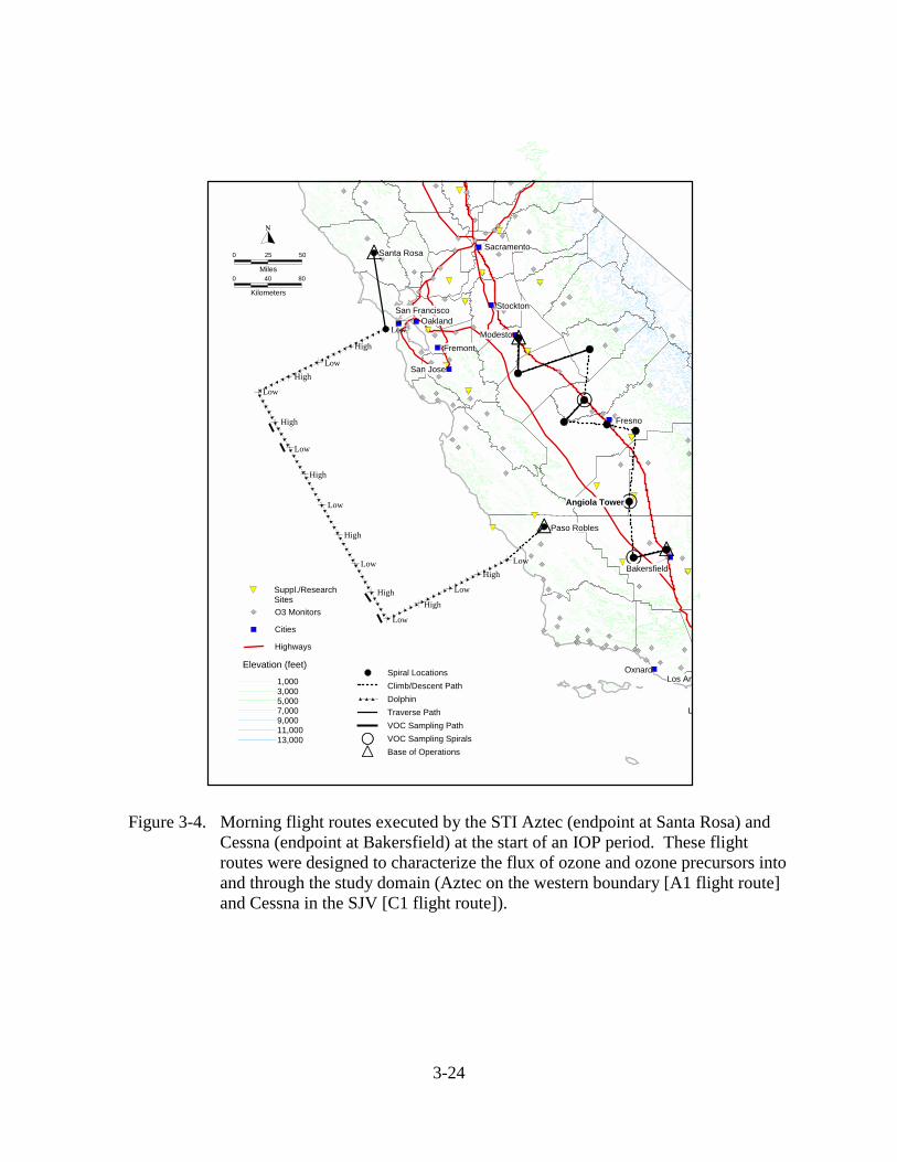
Figures 3-4 through 3-8 show the Aztec and Cessna morning and afternoon plannedflight paths. The maps include both the Aztec and Cessna flight routes that were executeddepending on the stage of the IOP. The first two maps (Figures 3-4 and 3-5) show the morningand afternoon routes flown at the start of an IOP. The next two maps (Figures 3-6 and 3-7) showthe flight routes executed as an ozone episode developed in the SJV. The final map (Figure 3-8)shows the flight routes executed when the ozone episode included both the Sacramento and SanJoaquin Valleys. Pass types (traverses, dolphins, and spirals) are indicated by various symbolson the planned flight path. Maps showing the actual sampling route flown during each STImission are included in Buhr et al., (2001).
3-14
Table 3-4. Flight plan A-1: Aztec Coastal Flight Plan, Santa Rosa to Paso Robles.
End Point Location
From To Pass TypeAltitude(ft msl)
HydrocarbonSampleAltitude(ft msl)
Distance(NM)
Latitude(deg.)
Longitude(deg.)
Santa Rosa (STS) Santa Rosa (STS) spiral to 4000 0 38.51 122.81Santa Rosa (STS) Offshore San Francisco traverse 5000 48 37.72 122.66Offshore San Francisco Offshore San Francisco spiral to 100 0 37.72 122.66Offshore San Francisco N. Offshore dolphin (2 cycles) 100-5000 84 37.07 124.30N. Offshore S. Offshore dolphin (4 cycles) 100-5000 cycles 1 and
4: 100-1000 &1500-2500
168 34.72 122.65
S. Offshore S. Shoreline dolphin (2 cycles) 100-5000 84 35.33 121.10S. Shoreline Paso Robles (PRB) climb 5000 30 35.67 120.63Paso Robles (PRB) Paso Robles (PRB) spiral to 100 0 35.67 120.63
3-15
Table 3-5. Flight plan A-2: Aztec Coastal Flight Plan, Paso Robles to Santa Rosa.
End Point Location
From To Pass TypeAltitude(ft msl)
HydrocarbonSample Altitude
(ft msl)Distance
(NM)Latitude(deg.)
Longitude(deg.)
Paso Robles (PRB) Paso Robles (PRB) spiral to 5000 0 35.67 120.63Paso Robles (PRB) S. Coastal descend to 100 30 35.33 121.20S. Coastal Offshore Carmel dolphin (2 cycles) 100-5000 cycle 1: 100-
1000 & 1500-2500
84 36.48 122.22
Offshore Carmel Offshore San Francisco (2) dolphin (2 cycles) 100-5000 cycle 2: 100-1000 & 1500-
2500
84 37.72 122.76
Offshore San Francisco (2) Point Arena dolphin (2 cycles) 100-5000 84 38.95 123.75Point Arena Ukiah (UKI) climb 6000 26 39.13 123.20Ukiah (UKI) Ukiah (UKI) spiral to 100 0 39.13 123.20Ukiah (UKI) Santa Rosa (STS) climb 5000 42 38.51 122.81Santa Rosa (STS) Santa Rosa (STS) spiral to 100 0 38.51 122.81
3-16
Table 3-6. Flight plan A-3: Aztec Northern Boundary Flight Plan, Santa Rosa to Modesto.
End Point Location
From To Pass TypeAltitude(ft MSL)
Hydrocarbon SampleAltitude (ft msl)
Distance(NM)
Latitude(deg.)
Longitude(deg.)
Santa Rosa (STS) Santa Rosa (STS) spiral to 5000 0 38.51 122.81Santa Rosa (STS) Ukiah (UKI) traverse 5000 40 39.13 123.20Ukiah (UKI) Ukiah (UKI) spiral to surface 0 39.13 123.20Ukiah (UKI) Willows (WLW) climb to 4000 52 39.52 122.22Willows (WLW) Willows (WLW) spiral to surface orbit @ 2500 0 39.52 122.22Willows (WLW) Redding (RDD) climb to 10000 62 40.51 122.29Redding (RDD) Redding (RDD) spiral to surface orbit @ 2500 & 1500-
surface0 40.51 122.29
Redding (RDD) Oroville (OVE) climb to 4000 70 39.49 121.62Oroville (OVE) Oroville (OVE) spiral to surface orbit @ 2500 0 39.49 121.62Oroville (OVE) Lodi (O20) climb to 4000 85 38.09 121.36Lodi (O20) Lodi (O20) spiral to surface 0 38.09 121.36Lodi (O20) Modesto (MOD) climb to 3000 34 37.63 120.95Modesto (MOD) Modesto (MOD) spiral to surface 0 37.63 120.95
3-17
Table 3-7. Flight plan A-4: Aztec Northern San Joaquin Valley Flight Plan, Santa Rosa to Modesto.
End Point Location
From To Pass TypeAltitude(ft msl)
Hydrocarbon SampleAltitude (ft msl)
Distance(NM)
Latitude(deg.)
Longitude(deg.)
Santa Rosa (STS) Santa Rosa (STS) spiral to 5000 0 38.51 122.81Santa Rosa (STS) Lodi (O20) traverse 5000 75 38.09 121.36Lodi (O20) Lodi (O20) spiral to surface 0 38.09 121.36Lodi (O20) Byron (4Q5) climb to 5000 20 37.84 121.64Byron (4Q5) Byron (4Q5) spiral to surface 0 37.84 121.64Byron (4Q5) Tracy (TCY) climb to 5000 12 37.69 121.44Tracy (TCY) Tracy (TCY) spiral to surface 0 37.69 121.44Tracy (TCY) NASA Crows Landing (NRC) climb to 5000 22 37.42 121.10NASA Crows Landing(NRC)
NASA Crows Landing (NRC) spiral to surface orbit @ 2500 & 1000-surface
0 37.42 121.10
NASA Crows Landing(NRC)
Gustine (3O1) climb to 5000 12 37.26 120.96
Gustine (3O1) Gustine (3O1) spiral to surface 0 37.26 120.96Gustine (3O1) Turlock (O15) climb to 5000 20 37.49 120.70Turlock (O15) Turlock (O15) spiral to surface orbit @ 2500 & 1150-
surface0 37.49 120.70
Turlock (O15) Don Pedro Reservoir climb to 5000 20 0.00 0.00Don Pedro Reservoir Don Pedro Reservoir spiral to surface 0 0.00 0.00Don Pedro Reservoir Oakdale (O27) climb to 5000 20 37.76 120.80Oakdale (O27) Oakdale (O27) spiral to surface 0 37.76 120.80Oakdale (O27) Modesto (MOD) climb to 5000 11 37.63 120.95Modesto (MOD) Modesto (MOD) spiral to surface 0 37.63 120.95
3-18
Table 3-8. Flight plan A-5: Aztec Northern San Joaquin Valley Flight Plan, Modesto to Santa Rosa.
End Point Location
From To Pass TypeAltitude(ft msl)
HydrocarbonSampleAltitude(ft msl)
Distance(NM)
Latitude(deg.)
Longitude(deg.)
Modesto (MOD) Modesto (MOD) spiral to 5000 0 37.63 120.95Modesto (MOD) Don Pedro Reservoir traverse 5000 28 37.73 120.40Don Pedro Reservoir Don Pedro Reservoir spiral to 900 0 37.73 120.40Don Pedro Reservoir Castle (MER) traverse 2500 21 37.38 120.57Castle Castle (MER) climb/spiral 5000-surface orbit @ 2500 0 37.38 120.57Castle Los Banos (LSN) traverse 2500 24 37.06 120.87Los Banos (LSN) San Luis Reservoir traverse 2500 12 121.12 37.05San Luis Reservoir San Luis Reservoir spiral to surface-5000 orbit @ 2500 0 121.12 37.05San Luis Reservoir San Martin (Q99) traverse 5000 22 37.08 121.60San Martin (Q99) San Martin (Q99) spiral to surface orbit @ 2500 0 37.08 121.60San Martin (Q99) NASA Crows Landing (NRC) climb 5000 5000 31 37.42 121.10NASA Crows Landing(NRC)
NASA Crows Landing (NRC) spiral to surface 0 37.42 121.10
NASA Crows Landing(NRC)
Tracy (TCY) traverse 2500 23 37.69 121.44
Tracy (TCY) Tracy (TCY) climb/spiral 5000-surface 0 37.69 121.44Tracy (TCY) Bethel Island traverse 2500 22 38.01 121.64Bethel Island Bethel Island climb/spiral 5000-surface 0 38.01 121.64Bethel Island Napa County (APC) traverse 2500 33 38.21 122.28Napa County (APC) Santa Rosa (STS) climb 5000 30 38.51 122.81Santa Rosa (STS) Santa Rosa (STS) spiral to surface 0 38.51 122.81
3-19
Table 3-9. Flight plan C-1: Cessna San Joaquin Valley Flight Plan, Bakersfield to Modesto.
End Point Location
From To Pass TypeAltitude(ft msl)
HydrocarbonSampleAltitude(ft msl)
Distance(NM)
Latitude(deg.)
Longitude(deg.)
Bakersfield (BFL) Bakersfield (BFL) spiral to 5000 0 35.43 119.06Bakersfield (BFL) Button Willow (L62) traverse 4000 23 35.35 119.48Button Willow (L62) Button Willow (L62) spiral to surface 1300-surface 0 35.35 119.48Button Willow (L62) Angiola traverse 2000 35 35.93 119.53Angiola Angiola spiral 500-4000 orbit @ 2500 0 35.93 119.53Angiola Reedley (O32) climb 5000 45 36.67 119.45Reedley (O32) Reedley (O32) spiral surface 0 36.67 119.45Reedley (O32) Fresno-Chandler (FCH) climb to 4000 22 36.73 119.82Fresno-Chandler (FCH) Fresno-Chandler (FCH) spiral to surface 0 36.73 119.82Fresno-Chandler (FCH) Mendota (Q84) climb 4000 28 36.76 120.37Mendota (Q84) Mendota (Q84) spiral to surface 0 36.76 120.37Mendota (Q84) Madera (MAE) traverse 2000 19 36.99 120.11Madera (MAE) Madera (MAE) spiral surface-4000 orbit @ 2500 0 36.99 120.11Madera (MAE) Mariposa (O68) climb 6000 32 37.51 120.04Mariposa (O68) Mariposa (O68) spiral to surface 0 37.51 120.04Mariposa (O68) Gustine (3O1) traverse 2000 46 37.26 120.96Gustine (3O1) Gustine (3O1) spiral surface-4000 0 37.26 120.96Gustine (3O1) Modesto (MOD) traverse 4000 22 37.63 120.95Modesto (MOD) Modesto (MOD) spiral to surface 0 37.63 120.95
3-20
Table 3-10. Flight plan C-2: Cessna San Joaquin Valley Flight Plan, Modesto to Bakersfield.
End Point Location
From To Pass TypeAltitude(ft msl)
HydrocarbonSampleAltitude(ft msl)
Distance(NM)
Latitude(deg.)
Longitude(deg.)
Modesto (MOD) Modesto (MOD) spiral to 5000 0 37.63 120.95Modesto (MOD) East Valley (Bonanza Hills) descend to 2500 32 37.66 120.23East Valley (Bonanza Hills) Mendota (Q84) traverse 2500 50 36.76 120.37Mendota (Q84) Mendota (Q84) spiral surface-5000 0 36.76 120.37Mendota (Q84) West Valley descend to 2500 14 36.65 120.67West Madera (MAE) traverse 2500 46 36.99 120.11Madera (MAE) East Valley traverse 2500 2500 20 37.02 119.67East Valley Selma (0Q4) traverse (circle) 2500 40 36.58 119.66Selma (0Q4) Reedley (O32) climb to 7000 12 36.67 119.45Reedley (O32) Reedley (O32) spiral to surface 0 36.67 119.45Reedley (O32) Kettleman City traverse 2500 46 36.02 119.97Kettleman City Angiola climb to 5000 22 35.93 119.53Angiola Angiola spiral to surface orbit @ 2500 0 35.93 119.53Angiola NE of Bakersfield traverse 2500 33 35.68 118.93NE of Bakersfield SE of Bakersfield traverse 2500 20 35.33 118.75SE of Bakersfield S of Bakersfield traverse 2500 2500 16 35.20 119.08S of Bakersfield Bakersfield (BFL) climb to 5000 15 35.43 119.06Bakersfield (BFL) Bakersfield (BFL) spiral to surface 0 35.43 119.06
3-21
Table 3-11. Flight plan C-3: Cessna San Joaquin Valley Flight Plan, Modesto to Bakersfield.
End Point Location
From To Pass TypeAltitude(ft msl)
HydrocarbonSampleAltitude(ft msl)
Distance(NM)
Latitude(deg.)
Longitude(deg.)
Modesto (MOD) Modesto (MOD) spiral to 5000 0 37.63 120.95Modesto (MOD) Mendota (Q84) traverse 2500 59 36.76 120.37Mendota (Q84) Mendota (Q84) spiral surface-5000 0 36.76 120.37Mendota (Q84) West Valley descend 2500 14 36.65 120.67West Valley Madera (MAE) traverse 2500 46 36.99 120.11Madera (MAE) East Valley traverse 2500 2500 20 37.02 119.67East Valley Selma (0Q4) traverse (circle) 2500 40 36.58 119.66Selma (0Q4) Reedley (O32) climb 7000 12 36.67 119.45Reedley (O32) Reedley (O32) spiral to surface 0 36.67 119.45Reedley (O32) Kettleman City traverse 2500 46 36.02 119.97Kettleman City Angiola climb 5000 22 35.93 119.53Angiola Angiola spiral to surface orbit @ 2500 0 35.93 119.53Angiola NE of Bakersfield traverse 2500 33 35.68 118.93NE of Bakersfield SE of Bakersfield traverse 2500 20 35.33 118.75SE of Bakersfield S of Bakersfield traverse 2500 2500 16 35.20 119.08S of Bakersfield South traverse 2500 9 35.02 119.05SS of Bakersfield Caliente traverse 2500 27 35.30 118.62Caliente Caliente climb / spiral 6000-2500 0 35.30 118.62Caliente Bakersfield (BFL) climb 5000 22 35.43 119.06Bakersfield (BFL) Bakersfield (BFL) spiral to surface 0 35.43 119.06
3-22
Table 3-12. Flight plan C-4: Cessna Southern San Joaquin Valley Flight Plan, Bakersfield to Paso Robles.
End Point Location
From To Pass TypeAltitude(ft msl)
HydrocarbonSample Altitude
(ft msl)Distance
(NM)Latitude(deg.)
Longitude(deg.)
Bakersfield (BFL) Bakersfield (BFL) spiral to 5000 0 35.43 119.06Bakersfield (BFL) Button Willow (L62) traverse 4000 23 35.35 119.48Button Willow (L62) Button Willow (L62) spiral to surface 1350-surface 0 35.35 119.48Button Willow (L62) Angiola traverse 2000 35 35.93 119.53Angiola Angiola spiral 500-4000 orbit @ 2500 0 35.93 119.53Angiola Reedley (O32) climb 5000 45 36.67 119.45Reedley (O32) Reedley (O32) spiral to surface 0 36.67 119.45Reedley (O32) Fresno-Chandler (FCH) climb 4000 22 36.73 119.82Fresno-Chandler (FCH) Fresno-Chandler (FCH) spiral to surface 0 36.73 119.82Fresno-Chandler (FCH) Madera (MAE) climb 5000 21 36.99 120.11Madera (MAE) Madera (MAE) spiral to surface orbit @ 2500 0 36.99 120.11Madera (MAE) Mendota (Q84) climb to 5000 19 36.76 120.37Mendota (Q84) Mendota (Q84) spiral to surface 0 36.76 120.37Mendota (Q84) Five Points climb to 5000 21 36.45 120.27Five Points Five Points spiral to surface 0 36.45 120.27Five Points San Ardo climb to 5000 39 36.03 120.92San Ardo San Ardo spiral to surface 0 36.03 120.92San Ardo Paso Robles (PRB) climb to 5000 27 35.67 120.63Paso Robles (PRB) Paso Robles (PRB) spiral to surface 0 35.67 120.63
3-23
Table 3-13. C-5 flight plan: Cessna Southern San Joaquin Valley Flight Plan, Paso Robles to Bakersfield.
End point location
From To Pass TypeAltitude(ft msl)
HydrocarbonSample Altitude
(ft msl)Distance
(NM)Latitude(deg.)
Longitude(deg.)
Paso Robles (PRB) Paso Robles (PRB) spiral to 5000 0 35.67 120.63Paso Robles (PRB) San Ardo traverse 5000 27 36.03 120.92San Ardo San Ardo spiral to surface 0 36.03 120.92San Ardo Coalinga (CLG) Climb 5000 28 36.16 120.36Coalinga (CLG) Coalinga (CLG) spiral to surface 0 36.16 120.36Coalinga (CLG) West Valley Climb 2500 31 36.65 120.67West Valley Madera (MAE) traverse 2500 46 36.99 120.11Madera (MAE) East Valley traverse 2500 2500 20 37.02 119.67East Valley Selma (0Q4 traverse 2500 40 36.58 119.66Selma (0Q4) Reedley (O32) Climb 7000 12 36.67 119.45Reedley (O32) Reedley (O32) spiral to surface 0 36.67 119.45Reedley (O32) Kettleman City traverse 2500 46 36.02 119.97Kettleman City Angiola Climb 5000 22 35.93 119.53Angiola Angiola spiral to surface orbit @ 2500 0 35.93 119.53Angiola NE of Bakersfield traverse 2500 34 35.68 118.93NE of Bakersfield SE of Bakersfield traverse 2500 20 35.33 118.75SE of Bakersfield S of Bakersfield traverse 2500 2500 16 35.20 119.08S of Bakersfield Bakersfield (BFL) Climb 5000 15 35.43 119.06Bakersfield (BFL) Bakersfield (BFL) spiral to surface 0 35.43 119.06
3-24
0
0
�
40
Kilometers
25
Miles80
50
xxxx
xxxx
xxxx
4444
4444
4444
4444
Fresno
Modesto
San Jose
Bakersfield
San FranciscoOakland
OxnardLos An
L
Angiola Tower
High
Fremont
Sacramento
Stockton
LowHigh
Low
High
Low
High
Low
High
Low
High
Low
Low
HighLow
High
Low
Santa Rosa
Paso Robles
Elevation (feet)
1,0003,0005,0007,0009,00011,00013,000
Spiral LocationsClimb/Descent Path
Traverse PathVOC Sampling Path
xxxx VOC Sampling Spirals4444 Base of Operations
Cities
Highways
O3 Monitors
Dolphin
Suppl./ResearchSites
Figure 3-4. Morning flight routes executed by the STI Aztec (endpoint at Santa Rosa) andCessna (endpoint at Bakersfield) at the start of an IOP period. These flightroutes were designed to characterize the flux of ozone and ozone precursors intoand through the study domain (Aztec on the western boundary [A1 flight route]and Cessna in the SJV [C1 flight route]).
3-25
Kilometers
40Miles
�
0 80
0 25 50
xxxx
4444
4444
4444
4444
OaklandSan FranciscoModesto
Fresno
San Jose
Bakersfield
OxnardLos Angeles
Long Beach
Fremont
Gle
Sacramento
Stockton
Paso Robles
Santa Rosa
Low
High
High
Low
High
Low
High
Low
High
Low
Ukiah
Elevation (feet)
1,0003,0005,0007,0009,00011,00013,000
Spiral LocationsClimb/Descent Path
Traverse PathVOC Sampling PathVOC Sampling SpiralsBase of Operations
Cities
Highways
O3 Monitors
Dolphin
Suppl./ResearchSites
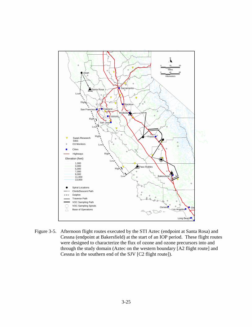
Figure 3-5. Afternoon flight routes executed by the STI Aztec (endpoint at Santa Rosa) andCessna (endpoint at Bakersfield) at the start of an IOP period. These flight routeswere designed to characterize the flux of ozone and ozone precursors into andthrough the study domain (Aztec on the western boundary [A2 flight route] andCessna in the southern end of the SJV [C2 flight route]).
3-26
Kilometers
40Miles
�
0 80
0 25 50
xxxx xxxx
xxxx
xxxx
xxxx
4444
4444
4444
4444
4444
4444
Angiola Tower
Fresno
ModestoOaklandSan Francisco
San Jose
Bakersfield
OxnardLos Angeles
Long Beach
Tracy
Gle
Sacramento
Stockton
Paso Robles
Santa Rosa
Elevation (feet)
1,0003,0005,0007,0009,00011,00013,000
Spiral LocationsClimb/Descent PathTraverse PathVOC Sampling PathVOC Sampling SpiralsBase of Operations
Cities
Highways
O3 Monitors
Suppl./Research Sites
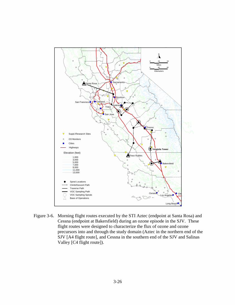
Figure 3-6. Morning flight routes executed by the STI Aztec (endpoint at Santa Rosa) andCessna (endpoint at Bakersfield) during an ozone episode in the SJV. Theseflight routes were designed to characterize the flux of ozone and ozoneprecursors into and through the study domain (Aztec in the northern end of theSJV [A4 flight route], and Cessna in the southern end of the SJV and SalinasValley [C4 flight route]).
3-27
Kilometers
40Miles
�
0 80
0 25 50
x
xx
4444
4444
xxxx
4444
4444
Bakersfield
Fresno
OaklandSan FranciscoModesto
San Jose
OxnardLos Angeles
Long Beach
Fremont
Gle
Sacramento
Stockton
Angiola Tower
Paso Robles
Santa Rosa
Elevation (feet)
1,0003,0005,0007,0009,00011,00013,000
Spiral LocationsClimb/Descent PathTraverse PathVOC Sampling PathVOC Sampling SpiralsBase of Operations
Cities
Highways
O3 Monitors
Suppl./Research Sites
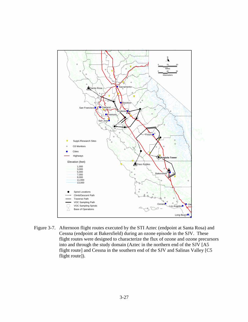
Figure 3-7. Afternoon flight routes executed by the STI Aztec (endpoint at Santa Rosa) andCessna (endpoint at Bakersfield) during an ozone episode in the SJV. Theseflight routes were designed to characterize the flux of ozone and ozone precursorsinto and through the study domain (Aztec in the northern end of the SJV [A5flight route] and Cessna in the southern end of the SJV and Salinas Valley [C5flight route]).
3-28
Kilometers
40Miles
�
0 80
0 25 50xxxx
xxxx
xxxx
xxxx
xxxx
xxxx
4444
4444
4444
4444
Angiola Tower
San Francisco
Fresno
ModestoOakland
San Jose
Bakersfield
Ukiah
Fremont
Sacramento
Stockton
Santa Rosa
Elevation (feet)
1,0003,0005,0007,0009,00011,00013,000
Spiral LocationsClimb/Descent PathTraverse PathVOC Sampling PathVOC Sampling SpiralsBase of Operations
Cities
Highways
O3 Monitors
Suppl./Research Sites
Figure 3-8. Morning flight routes executed by the STI Aztec (endpoint at Santa Rosa)and Cessna (endpoint at Bakersfield) during an ozone episode that includedthe Sacramento and San Joaquin Valleys. These flight routes were designedto characterize the flux of ozone and ozone precursors into and through thestudy domain (Aztec in the Sacramento Valley [A3 flight route] and Cessna inthe southern end of the SJV [C1 flight route]). The afternoon flight routes forthis scenario were the same as those shown in Figure 3-7 for the Aztec and inFigure 3-5 for the Cessna.
4-1
4. DATA PROCESSING, FORMATS, AND AVAILABILITY
4.1 DATA PROCESSING
Data documentation began before take-off and continued throughout each flight. Duringa flight, the sampling instrumentation and the data acquisition system (DAS) were runcontinuously. A flight consisted of a sequential series of sampling events that included zeroinginstruments before takeoff and after landing, spirals, traverses, and dolphins. These samplingevents (excluding instrument zeroing) were called "passes" and were numbered sequentiallyfrom the beginning of each flight, starting at one. Each flight was processed as a series ofpasses.
Aboard the aircraft, the on-board scientist (instrument operator) controlled an eventswitch that was used to flag passes. The data flag was recorded by the DAS and used during dataprocessing steps to identify various sections of data.
During each flight, the operator filled out standardized flight record sheets (flight notes)that summarized each pass. During data processing, the information contained in the flight noteswas checked against the flags and other data that were recorded by the DAS.
Initial processing of the data began after the aircraft returned to the base of operations atthe end of a sampling day. The objective was to provide a quick review of the data and toidentify and correct problems if they existed. The following processing was performed in thefield:
• The sampling date, the sampling period (start- and end-times), and the Zip diskidentification number were determined from flight notes and compared with theinformation recorded on the data disk. Differences were reconciled and corrected beforeother processing steps were initiated.
• During sampling, the continuous sensor data were written to the DAS's hard drive and toa removable backup Zip disk .
• After the flight, a data-processing program was used to read the raw ASCII data files andgenerate QC values (flags) that were added to the engineering unit file and accompaniedeach measurement value through all remaining processing steps. Initially these QCvalues were set to zero by the processing program, indicating that each data point wasvalid. If later editing changes were made to a data point, the associated QC value wasautomatically changed to reflect the editing that was performed.
• The processing program also produced a summary of times at which the event switch(recorded by the DAS) was activated or changed. This file was called an “eventsummary file”.
• The status of the event switch (from the event summary) was compared to the instrumentoperator's written flight notes, and discrepancies were noted. Appropriate correctiveactions were taken.
4-2
• The aircraft field manager reviewed each recorded parameter of the raw engineering unitdata using the on-screen display function of an editing program.
• Copies of the aircraft data file, the converted raw voltage file, the converted rawengineering unit file, and flight notes were returned to STI for further processing.
At STI the following processing was performed:
• Review and interactive editing of the raw engineering unit data were performed using anediting program. One element of the editing program was the creation (and continualupdating) of a separate log file that documented each processing step and logged allcorrections that were made.
• The data were reviewed for outliers (typically due to aircraft radio transmissions). Theseoutliers were marked using the editor and then invalidated.
• The editing program was used to add two calculated data fields to the flight data.Altitude in m msl (based on altitude in ft msl), absolute humidity (based on temperature,dew point, and pressure). Each data field had a QC field associated with it. If laterediting changes were made to a base measurement, the editing program automaticallyupdated the calculated data field and its QC flags.
• The type of sampling (spiral, traverse, or dolphin) performed during a pass and thelocation of the sampling (three-letter identifier) were added to the data file using theediting program.
• Using the event summary and flight notes, a tabular sampling summary was produced forinclusion with the data from each flight.
• Instrument calibration data were reviewed, and calibration factors were selected. Pre-and post-flight instrument zero values were checked and compared to calibration values.
• The editing program was used to apply zero values, calibration factors, offsets, andaltitude correction factors (when appropriate) to the raw engineering unit data. Eachcorrection or adjustment was automatically recorded in the editing program log file, andQC flags were changed appropriately.
• At this point, preliminary data plots were produced. Using the preliminary data plots,flight maps, sampling summaries, processing notes, and flight notes, a data processingsystem review was performed.
• Dates, times, locations, and the types of sampling for each pass were checked for each ofthe various outputs. The plotted data for each measurement were reviewed, andrelationships between parameters (e.g., NO/NOy ratios, etc.) were examined.
• Problems that existed were corrected. Most problems detected were clerical in nature(wrong end point number on the sampling summary, etc.) and were easily corrected.
• After all editing had been completed, final data plots were produced.
• After completion of all processing and editing, the final engineering unit data werecopied to permanent storage media (CD-ROM).
4-3
• Finally, both the data and QC values were translated to the CCAQS data submittal formatand transferred via FTP to ARB.
4.2 DATA FORMATS AND AVAILABILITY
The continuous sensor data have been reported to the ARB in the two-volume data reportby Blumenthal et al.(2001). The report contains a separate section for each flight. Each sectioncontains a sampling summary such as the one shown in Figure 4-1. The summary details thesampling locations, times, and information concerning the sampling that was performed. Thesummary also shows sample identifiers, locations, times, and altitudes for each integrated VOCand carbonyl grab sample collected. A sampling route map (Figure 4-2) follows the summarypage. Figures 4-3 and 4-4 are examples of data plots for individual passes conducted during aflight
The data plots present "snapshot" views for each pass of a flight. Some portions of data(e.g., while the aircraft was repositioning for the next pass) were not plotted, but these data arecontained in the data files that were delivered to the ARB.
The data were provided to the ARB in two formats. First the data were formattedaccording to the ARB CCAQS data transmittal instructions (California Air Resources Board,2001) and transferred to the ARB via ftp. In addition, the data were provided electronically on acompact disk (CD) in the format described below. The CD entitled “The real-time measurementdata collected aboard the STI aircraft during CCOS sampling” contains the aloft continuous airquality data collected aboard the STI aircraft.
The data files are in a tab-delimited text file format compatible with DOS-basedcomputers. Each variable occupies one column, and columns are separated by tab characters.The chosen format allows the user to read the data with either commercial software(e.g., spreadsheets such as MS Excel and word processors such as WordPerfect) orcustom-programmed software (e.g., FORTRAN-based programs).
The data files were named using the following convention:
Format: AircraftYear_Month_Day_Starttime.datAircraft = Aztec or Cessna
Year = 2000
Month = 7 (July), 8 (August), 9 (September)
Day = day of the month
Starttime = Starttime of the raw data in HHMM.*
Extension .dat = text file
* Leading and trailing zeros were not included in the file name starttime field.
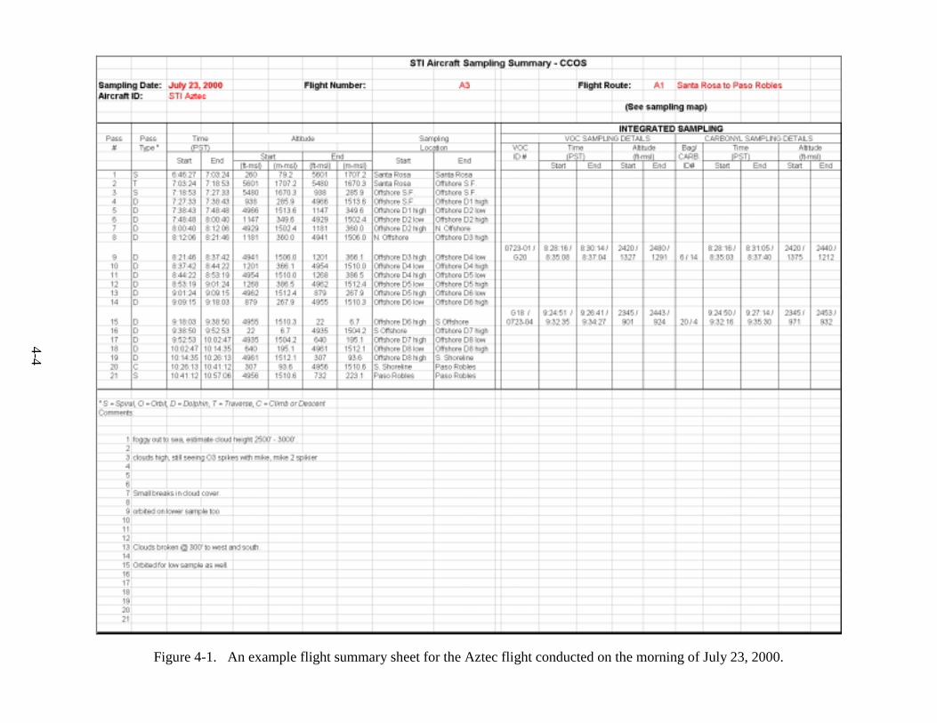
4-4
Figure 4-1. An example flight summary sheet for the Aztec flight conducted on the morning of July 23, 2000.
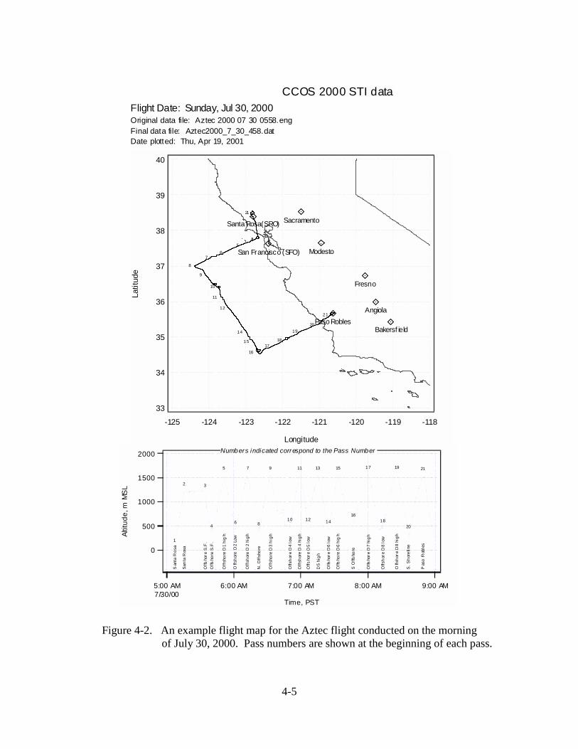
4-5
40
39
38
37
36
35
34
33
Latit
ude
-125 -124 -123 -122 -121 -120 -119 -118
Longitude
Bakersf ieldPaso Robles
Angiola
San Francisco (SFO)
Santa Rosa(SRO)
Fresno
Modesto
Sacramento12
345
67
8
9
10
11
12
14
15
1617
18
1920
21
2000
1500
1000
500
0
Altit
ude,
m M
SL
5:00 AM7/30/00
6:00 AM 7:00 AM 8:00 AM 9:00 AM
Time, PST
1
2 3
4
5
6
7
8
9
10
11
12
13
14
15
16
17
18
19
20
21
San
ta R
osa
Sant
a R
osa
Offs
hore
S.F
.O
ffsho
re S
.F.
Offs
hore
D1
hig
h
Offs
hore
D2
Low
Offs
hore
D2
high
N. O
ffsho
re
Offs
hore
D3
high
Offs
hore
D4
low
Offs
hore
D4
high
Offs
hore
D5
low
D5
high
Offs
hore
D6
low
Offs
hore
D6
hig
h
S O
ffsho
re
Offs
hore
D7
high
Offs
hore
D8
low
Offs
hore
D8
high
S. S
hore
line
Pas
o R
oble
s
Numbers indicated correspond to the Pass Number
CCOS 2000 STI dataFlight Date: Sunday, Jul 30, 2000Original data file: Aztec 2000 07 30 0558.eng
Date plotted: Thu, Apr 19, 2001Final data file: Aztec2000_7_30_458.dat
Figure 4-2. An example flight map for the Aztec flight conducted on the morningof July 30, 2000. Pass numbers are shown at the beginning of each pass.
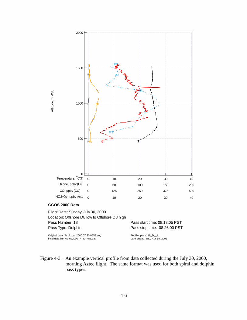
4-6
Figure 4-3. An example vertical profile from data collected during the July 30, 2000,morning Aztec flight. The same format was used for both spiral and dolphinpass types.
2000
1500
1000
500
0
Alti
tude
,m M
SL
5003752501250CO, ppbv (CO)
403020100NO,NOy, ppbv (N,Ny)
403020100Temperature, oC(T)
200150100500Ozone, ppbv (O)
CO
CO
CO
CO
CO
Ny
Ny
Ny
N
N
N
T
T
T
O
O
O
CCOS 2000 Data
Original data f ile: Aztec 2000 07 30 0558.eng
Flight Date: Sunday, July 30, 2000Location: Offshore D8 low to Offshore D8 highPass Number: 18Pass Type: Dolphin
Pass start time: 08:13:05 PSTPass stop time: 08:26:00 PST
Final data f ile: Aztec2000_7_30_458.dat Date plotted: Thu, Apr 19, 2001Plot f ile: pass118_D__1
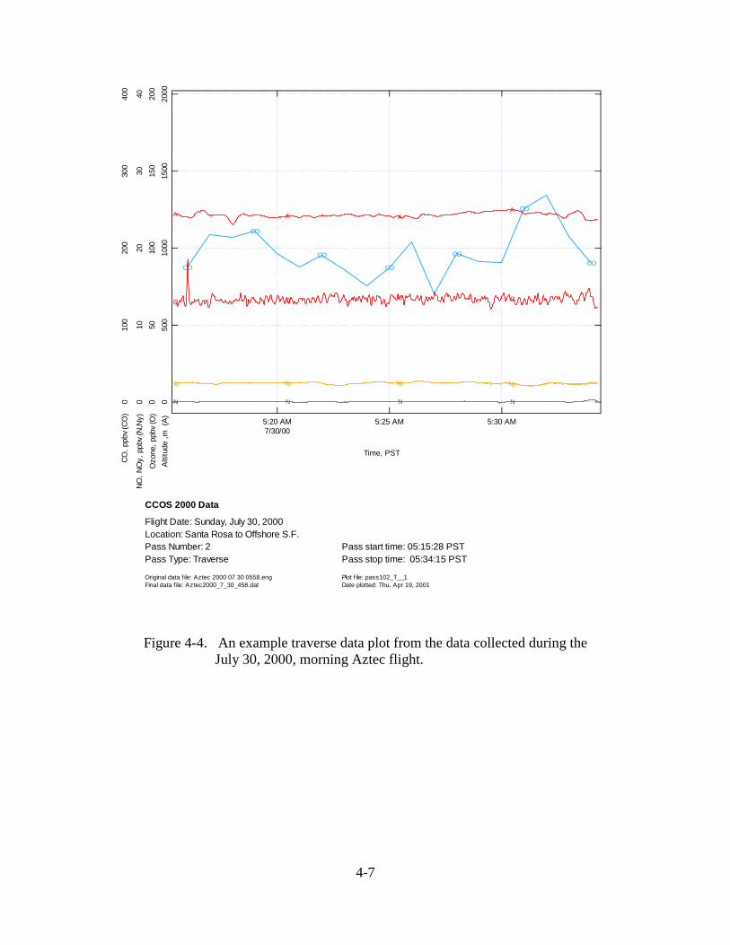
4-7
400
300
200
100
0CO
, ppb
v (CO
)
5:20 AM7/30/00
5:25 AM 5:30 AM
Time, PST
4030
2010
0NO
, NO
y, p
pbv
(N,N
y)
2000
1500
1000
500
0Al
titud
e ,m
(A)
200
150
100
500
Ozo
ne, p
pbv
(O)
CO
CO
CO
CO
CO
CO
CO
N N N N
Ny Ny Ny Ny
A A AA
O O O O
CCOS 2000 Data
Original data f ile: Aztec 2000 07 30 0558.eng
Flight Date: Sunday, July 30, 2000Location: Santa Rosa to Offshore S.F.Pass Number: 2Pass Type: Traverse
Pass start time: 05:15:28 PSTPass stop time: 05:34:15 PST
Final data f ile: Aztec2000_7_30_458.dat Date plotted: Thu, Apr 19, 2001Plot f ile: pass102_T__1
Figure 4-4. An example traverse data plot from the data collected during theJuly 30, 2000, morning Aztec flight.
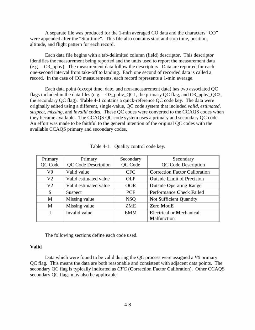
4-8
A separate file was produced for the 1-min averaged CO data and the characters “CO”were appended after the “Starttime”. This file also contains start and stop time, position,altitude, and flight pattern for each record.
Each data file begins with a tab-delimited column (field) descriptor. This descriptoridentifies the measurement being reported and the units used to report the measurement data(e.g. – O3_ppbv). The measurement data follow the descriptors. Data are reported for eachone-second interval from take-off to landing. Each one second of recorded data is called arecord. In the case of CO measurements, each record represents a 1-min average.
Each data point (except time, date, and non-measurement data) has two associated QCflags included in the data files (e.g. – O3_ppbv_QC1, the primary QC flag, and O3_ppbv_QC2,the secondary QC flag). Table 4-1 contains a quick-reference QC code key. The data wereoriginally edited using a different, single-value, QC code system that included valid, estimated,suspect, missing, and invalid codes. These QC codes were converted to the CCAQS codes whenthey became available. The CCAQS QC code system uses a primary and secondary QC code.An effort was made to be faithful to the general intention of the original QC codes with theavailable CCAQS primary and secondary codes.
Table 4-1. Quality control code key.
PrimaryQC Code
PrimaryQC Code Description
SecondaryQC Code
SecondaryQC Code Description
V0 Valid value CFC Correction Factor CalibrationV2 Valid estimated value OLP Outside Limit of PrecisionV2 Valid estimated value OOR Outside Operating RangeS Suspect PCF Performance Check FailedM Missing value NSQ Not Sufficient QuantityM Missing value ZME Zero ModEI Invalid value EMM Electrical or Mechanical
Malfunction
The following sections define each code used.
Valid
Data which were found to be valid during the QC process were assigned a V0 primaryQC flag. This means the data are both reasonable and consistent with adjacent data points. Thesecondary QC flag is typically indicated as CFC (Correction Factor Calibration). Other CCAQSsecondary QC flags may also be applicable.
4-9
Valid – Estimated
Data points which were calculated from other data or which were estimated based onavailable calibrations are marked by a V2 primary QC flag. Depending on the reason forassigning the estimated primary QC flag, the secondary QC flag is indicated as either OLP(Outside Limit of Precision) or OOR (Outside Operating Range).
Suspect
Data points that were judged to be suspect were assigned the S primary QC flag and thePCF (Performance Check Failed ) secondary QC flag.
Missing
Data that for some reason were missing from the data file (inoperative analyzer, lost data)were assigned a primary QC flag M (Missing value), and a secondary QC flag NSQ (NotSufficient Quantity). The M primary QC flag was also used for zero mode data according to theCCAQS convention. In this case the secondary QC flag was assigned as ZME (Zero ModE).As for invalid data, the value of the parameter in the data file was replaced by null.Two copies of the data report and CD were delivered to the ARB. Copies of the final processeddata, individual log files, the original data from the aircraft, and processing notes are stored inarchive files at STI. These archives will be maintained for at least five years.
Invalid
Data points which were not reasonable from either a scientific or an engineeringstandpoint were assigned an I (Invalid) primary QC flag and the EMM (Electrical or MechanicalMalfunction) secondary QC flag. The value of the parameter in the data file was replaced bynull. For example, noise or radio-frequency interference from the aircraft communicationsequipment sometimes generated "spikes" in some of the data points. These data, which wereobviously erroneous, were marked as invalid.
5-1
5. DATA QUALITY
Quality control (QC) procedures are discussed in this report in terms of activitiesperformed by STI to assure the quality of the aircraft data. Actions taken by others to assure thequality of the aircraft data are discussed as quality assurance (QA) activities. For example,instrument calibrations were an STI QC activity; but, the performance audit by the ARB was aQA activity.
5.1 QUALITY CONTROL
5.1.1 Pre-program Quality Control Measures
The following activities were performed by STI before the start of the program to controlthe quality of the aircraft data:
• Checklists and log sheets, specific to the instruments and sampling systems operatedaboard the aircraft, were designed. These were used throughout the program tostandardize operational procedures and to document all activities relating to themeasurements.
• Operational bases at the Santa Rosa, Bakersfield, Modesto, and Paso Robles airportswere established. Arrangements were made to install needed power circuits at eachfacility.
• Prior to transfer to Santa Rosa and Bakersfield from the Healdsburg airport, each piece ofsampling equipment to be used aboard the two aircraft was cleaned, checked, andcalibrated. New inlet particulate filters and sample lines were installed in the samplinginstruments.
• The aircraft were instrumented and test flights were flown. Data recorded during theseflights were processed and reviewed to ensure that the complete instrumentation package,or system, was operational.
• The calibration systems and an ozone transfer standard (UV photometer) were checkedand certified. NIST-certified calibration gas was ordered and delivered to the Santa Rosaand Bakersfield base facilities.
• Aircraft sampling routes were discussed with the FAA and other airport facilities toensure that desired sampling could be performed. Necessary certifications and waiverswere obtained from the FAA.
• A performance audit of the gas monitors (while mounted in the aircraft) was performedon June 19 and July 3, 2001. The audit results are described in Section 5.2.
• The Aztec flew an intercomparison flight with the DOE G-1 aircraft on July 5, 2000.
• Both the Aztec and Cessna 182 flew an intercomparison flight with the UCD 182 onJuly 6, 2000.
5-2
5.1.2 Quality Control Measures During the Field Program
Many checks, procedures, and instrument backups combined to assure the quality of theaircraft data:
• Backup instruments (ozone and NO/NOy) were maintained at STI. These instrumentswere calibrated and made ready to be installed in either aircraft, when needed.
• At all four fixed bases of operations, air conditioning was provided to the aircraft toreduce heat loading between flights or IOPs.
• Instruments requiring warm-up periods were turned on after arriving in the field and wereoperated continuously throughout the remainder of the program in order to maintain theircalibrations. When the aircraft landed at the Modesto or Paso Robles airports, thenecessary power, hangar, and air conditioning was available to the instrumentation whilethe aircraft was between flights.
• All sampling coordinates were entered into the GPS unit aboard the aircraft.
• Inlet particle filters were changed periodically throughout the program. Fixed instrumentranges were used for the continuous monitors throughout the sampling program.
• Aircraft sampling system checks were conducted each day and prior to and followingscheduled/completed flights.
• Multi-point calibrations of the air quality instruments were performed prior to andfollowing most flight days. Additional details and the results of these calibrationactivities are reported in Section 5.1.3.
• To detect systematic calibration errors, the instruments were calibrated by differentmembers of the aircraft crew on different days.
• A detailed checklist was used to perform extensive operational checks on each instrumentprior to each sampling flight.
• Data were recorded on the data acquisition computer’s hard disk drive and on aremovable, backup ZIP disk simultaneously to provide redundancy.
• The aircraft field manager debriefed flight crews after each flight to identify and, ifnecessary, correct any operational problems.
• Data files and flight notes were copied after each flight. The data were carefullyreviewed by the aircraft field manager to identify any problems. Problems that werenoted were discussed with the flight crew(s).
• After a flight was completed, flight notes were reviewed and VOC and carbonyl grabsamples were inventoried and periodically delivered to the appropriate contractors.
• After a carbonyl grab sample had been collected, the sample bag was placed inside alarger opaque bag.
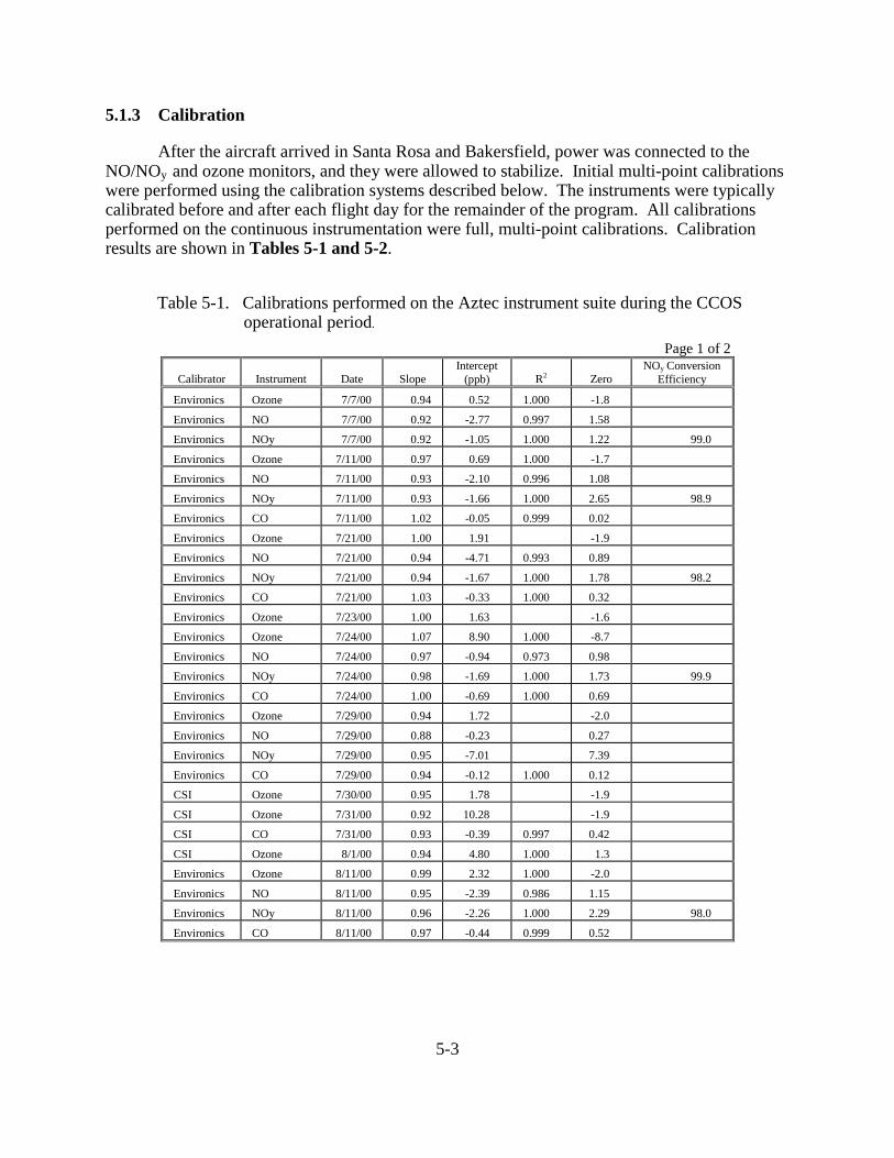
5-3
5.1.3 Calibration
After the aircraft arrived in Santa Rosa and Bakersfield, power was connected to theNO/NOy and ozone monitors, and they were allowed to stabilize. Initial multi-point calibrationswere performed using the calibration systems described below. The instruments were typicallycalibrated before and after each flight day for the remainder of the program. All calibrationsperformed on the continuous instrumentation were full, multi-point calibrations. Calibrationresults are shown in Tables 5-1 and 5-2.
Table 5-1. Calibrations performed on the Aztec instrument suite during the CCOSoperational period.
Page 1 of 2
Calibrator Instrument Date SlopeIntercept
(ppb) R2 ZeroNOy Conversion
Efficiency
Environics Ozone 7/7/00 0.94 0.52 1.000 -1.8
Environics NO 7/7/00 0.92 -2.77 0.997 1.58
Environics NOy 7/7/00 0.92 -1.05 1.000 1.22 99.0
Environics Ozone 7/11/00 0.97 0.69 1.000 -1.7
Environics NO 7/11/00 0.93 -2.10 0.996 1.08
Environics NOy 7/11/00 0.93 -1.66 1.000 2.65 98.9
Environics CO 7/11/00 1.02 -0.05 0.999 0.02
Environics Ozone 7/21/00 1.00 1.91 -1.9
Environics NO 7/21/00 0.94 -4.71 0.993 0.89
Environics NOy 7/21/00 0.94 -1.67 1.000 1.78 98.2
Environics CO 7/21/00 1.03 -0.33 1.000 0.32
Environics Ozone 7/23/00 1.00 1.63 -1.6
Environics Ozone 7/24/00 1.07 8.90 1.000 -8.7
Environics NO 7/24/00 0.97 -0.94 0.973 0.98
Environics NOy 7/24/00 0.98 -1.69 1.000 1.73 99.9
Environics CO 7/24/00 1.00 -0.69 1.000 0.69
Environics Ozone 7/29/00 0.94 1.72 -2.0
Environics NO 7/29/00 0.88 -0.23 0.27
Environics NOy 7/29/00 0.95 -7.01 7.39
Environics CO 7/29/00 0.94 -0.12 1.000 0.12
CSI Ozone 7/30/00 0.95 1.78 -1.9
CSI Ozone 7/31/00 0.92 10.28 -1.9
CSI CO 7/31/00 0.93 -0.39 0.997 0.42
CSI Ozone 8/1/00 0.94 4.80 1.000 1.3
Environics Ozone 8/11/00 0.99 2.32 1.000 -2.0
Environics NO 8/11/00 0.95 -2.39 0.986 1.15
Environics NOy 8/11/00 0.96 -2.26 1.000 2.29 98.0
Environics CO 8/11/00 0.97 -0.44 0.999 0.52
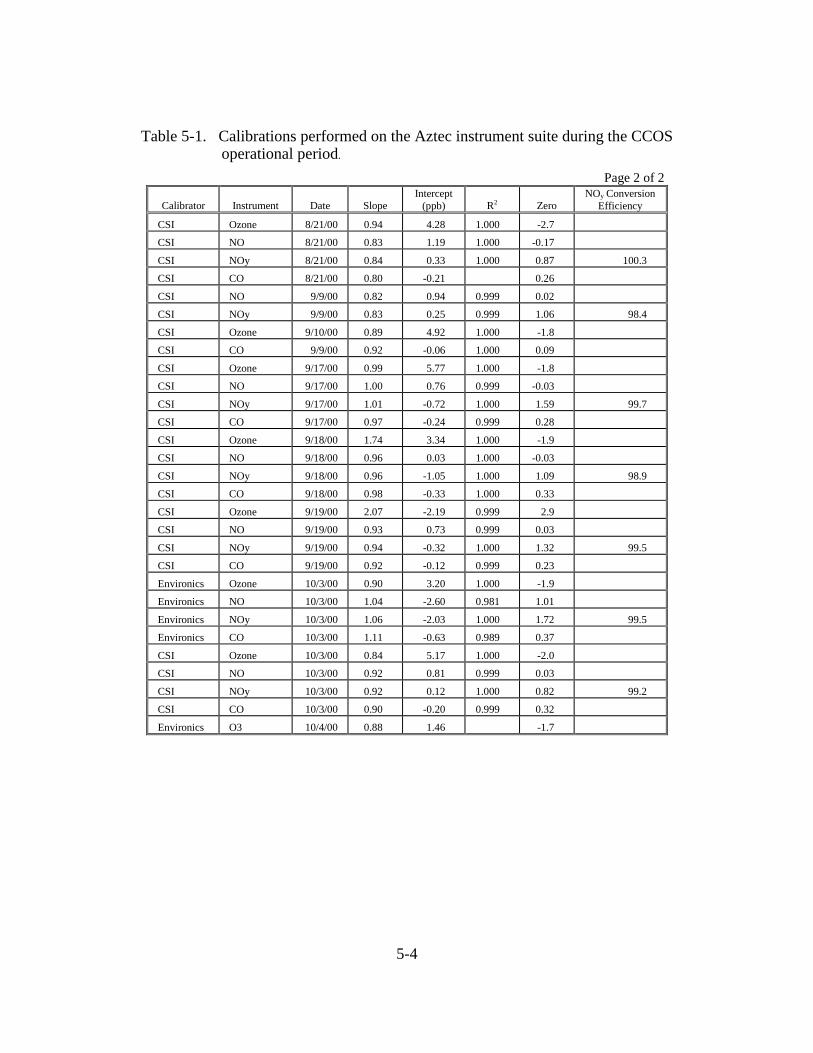
5-4
Table 5-1. Calibrations performed on the Aztec instrument suite during the CCOSoperational period.
Page 2 of 2
Calibrator Instrument Date SlopeIntercept
(ppb) R2 ZeroNOy Conversion
Efficiency
CSI Ozone 8/21/00 0.94 4.28 1.000 -2.7
CSI NO 8/21/00 0.83 1.19 1.000 -0.17
CSI NOy 8/21/00 0.84 0.33 1.000 0.87 100.3
CSI CO 8/21/00 0.80 -0.21 0.26
CSI NO 9/9/00 0.82 0.94 0.999 0.02
CSI NOy 9/9/00 0.83 0.25 0.999 1.06 98.4
CSI Ozone 9/10/00 0.89 4.92 1.000 -1.8
CSI CO 9/9/00 0.92 -0.06 1.000 0.09
CSI Ozone 9/17/00 0.99 5.77 1.000 -1.8
CSI NO 9/17/00 1.00 0.76 0.999 -0.03
CSI NOy 9/17/00 1.01 -0.72 1.000 1.59 99.7
CSI CO 9/17/00 0.97 -0.24 0.999 0.28
CSI Ozone 9/18/00 1.74 3.34 1.000 -1.9
CSI NO 9/18/00 0.96 0.03 1.000 -0.03
CSI NOy 9/18/00 0.96 -1.05 1.000 1.09 98.9
CSI CO 9/18/00 0.98 -0.33 1.000 0.33
CSI Ozone 9/19/00 2.07 -2.19 0.999 2.9
CSI NO 9/19/00 0.93 0.73 0.999 0.03
CSI NOy 9/19/00 0.94 -0.32 1.000 1.32 99.5
CSI CO 9/19/00 0.92 -0.12 0.999 0.23
Environics Ozone 10/3/00 0.90 3.20 1.000 -1.9
Environics NO 10/3/00 1.04 -2.60 0.981 1.01
Environics NOy 10/3/00 1.06 -2.03 1.000 1.72 99.5
Environics CO 10/3/00 1.11 -0.63 0.989 0.37
CSI Ozone 10/3/00 0.84 5.17 1.000 -2.0
CSI NO 10/3/00 0.92 0.81 0.999 0.03
CSI NOy 10/3/00 0.92 0.12 1.000 0.82 99.2
CSI CO 10/3/00 0.90 -0.20 0.999 0.32
Environics O3 10/4/00 0.88 1.46 -1.7
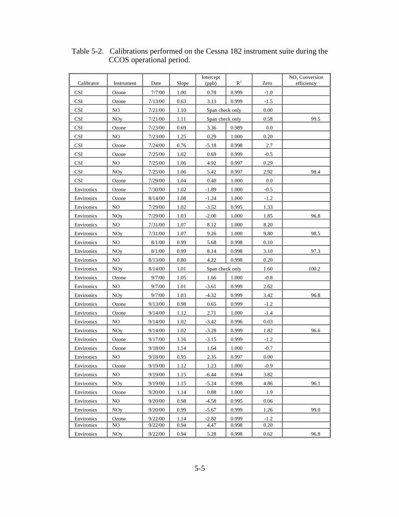
5-5
Table 5-2. Calibrations performed on the Cessna 182 instrument suite during theCCOS operational period.
Calibrator Instrument Date SlopeIntercept
(ppb) R2 ZeroNOy Conversion
efficiency
CSI Ozone 7/7/00 1.00 0.78 0.999 -1.0
CSI Ozone 7/13/00 0.63 3.13 0.999 -1.5
CSI NO 7/21/00 1.10 Span check only 0.00
CSI NOy 7/21/00 1.11 Span check only 0.58 99.5
CSI Ozone 7/23/00 0.69 3.36 0.989 0.0
CSI NO 7/23/00 1.25 0.29 1.000 0.20
CSI Ozone 7/24/00 0.76 -5.18 0.998 2.7
CSI Ozone 7/25/00 1.02 0.69 0.999 -0.5
CSI NO 7/25/00 1.06 4.92 0.997 0.29
CSI NOy 7/25/00 1.06 5.42 0.997 2.92 98.4
CSI Ozone 7/29/00 1.04 0.40 1.000 0.0
Environics Ozone 7/30/00 1.02 -1.89 1.000 -0.5
Environics Ozone 8/14/00 1.08 -1.24 1.000 -1.2
Environics NO 7/29/00 1.02 -3.52 0.995 1.33
Environics NOy 7/29/00 1.03 -2.00 1.000 1.85 96.8
Environics NO 7/31/00 1.07 8.12 1.000 8.20
Environics NOy 7/31/00 1.07 9.26 1.000 9.80 98.5
Environics NO 8/1/00 0.99 5.68 0.998 0.10
Environics NOy 8/1/00 0.99 8.14 0.998 3.10 97.3
Environics NO 8/13/00 0.80 4.22 0.998 0.20
Environics NOy 8/14/00 1.01 Span check only 1.60 100.2
Environics Ozone 9/7/00 1.05 1.66 1.000 -0.8
Environics NO 9/7/00 1.01 -3.61 0.999 2.62
Environics NOy 9/7/00 1.03 -4.32 0.999 3.42 96.8
Environics Ozone 9/13/00 0.98 0.65 0.999 -1.2
Environics Ozone 9/14/00 1.12 2.71 1.000 -1.4
Environics NO 9/14/00 1.02 -3.42 0.996 0.03
Environics NOy 9/14/00 1.02 -3.28 0.999 1.82 96.6
Environics Ozone 9/17/00 1.16 -3.15 0.999 -1.2
Environics Ozone 9/18/00 1.14 1.64 1.000 -0.7
Environics NO 9/18/00 0.95 2.35 0.997 0.00
Environics Ozone 9/19/00 1.12 1.23 1.000 -0.9
Environics NO 9/19/00 1.15 -6.44 0.994 3.82
Environics NOy 9/19/00 1.15 -5.24 0.998 4.86 96.1
Environics Ozone 9/20/00 1.14 0.88 1.000 1.9
Environics NO 9/20/00 0.98 -4.58 0.995 0.06
Environics NOy 9/20/00 0.99 -5.67 0.999 1.26 99.0
Environics Ozone 9/22/00 1.14 -2.82 0.999 -1.2Environics NO 9/22/00 0.94 4.47 0.998 0.20
Environics NOy 9/22/00 0.94 5.28 0.998 0.62 96.8
5-6
In processing the data, the calibration history of a particular instrument was consideredbefore applying the appropriate sensitivity slope and zero offset to the data. If the results of acalibration showed either a sensitivity or zero offset that was not consistent with previous orsubsequent calibrations, a decision was made whether to use that calibration data or to applyvalues consistent with the neighboring calibrations. The calibration values were applied usingthe following formula:
Calibrated_measurand = (measurand + zero_offset) * slope.
Calibration equipment
The dynamic calibration system for each aircraft consisted of a portable calibrator, a zeroair system/module (ZAM), an ozone transfer standard, and a NIST-traceable gas cylindercontaining a certified level of NO, SO2, and CO in nitrogen. The calibrators used alternatelywith both aircraft were an Environics Series 100 and a Columbia Scientific Industries (CSI)Model 1700. Each calibrator contained two mass flow controllers which provided known flowrates of dilution air from the ZAM and span gas from the standard gas cylinder. The calibratorwas capable of delivering the desired gas concentrations by adjusting each mass flow controllerto provide previously determined flow rates. The dilution airflow controller had a nominal rangeof 1,000 to 10,000 standard cubic centimeters per minute (sccm), and the span gas flowcontroller had a nominal range of 5 to 100 sccm.
Each calibrator contained an ozone generator, which was used for ozone calibrations.The ozone stream could be directed into the dilution air stream to enable these calibrations.Gas-phase titration (GPT) could also be performed by directing the ozone stream into the NOspan gas stream. Each calibrator had a reaction chamber and a mixing chamber of appropriatedimensions, which, when taken together with the flow rates that were used, complied with theU.S. Environmental Protection Agency (EPA) requirements for NO2 generation by means of theGPT procedure.
As required by the EPA, high concentration span gases came in contact with onlystainless steel, Teflon, and glass. Diluted gases came in contact with only Teflon and glass andwere sampled from the calibrator at ambient pressure by means of a small sample manifold, towhich the calibrator effluent and analyzer sample line were connected.
Zero air module
Zero air for the calibrator was generated from ambient air using a portable ZAM. TheZAM contained a compressor, a drier, Purafil, activated charcoal, Hopcalite, and a 5-micronmolecular sieve particle filter. The ZAM delivered dry air, which was free of NO, NO2, andozone, at a flow and pressure which met the specifications of the dilution mass flow controller inthe calibrator.
5-7
Compressed gas standard
The NIST-traceable NO and CO span gas cylinders used during the project werepurchased from Scott-Marrin, Inc. These cylinders were used with the dilution calibrators tocalibrate the NO/NOy and the CO (Aztec only) analyzers.
Ozone transfer standard
A Dasibi 1003 was used as a transfer standard for both aircraft at the start of the program.It was traceable to a primary standard and was certified using the primary standard. Ozoneconcentrations generated by the CSI calibrator were measured using the transfer standard. TheEnvironics calibrator provided a direct readout of the ozone concentration generated.
Procedures
The calibrator and transfer standard were checked and tested by STI’s QA laboratory inBakersfield prior to use in the program. Mass flow controllers received multi-point flow checks.The ozone transfer standard was certified against a primary standard before the program andagain after the program.
For ozone calibration, the sample delivery line from the calibrator was connected to theinlet of the glass manifold inside the aircraft. The analyzer sampled normally from the glassmanifold. Temperature (in the photometer cell) and pressure measurements were made duringcalibrations and were applied to calculations to determine true ozone concentrations.
For calibration of the NO analyzers, the sample delivery line from the calibrator wasconnected to what was normally the exhaust port of one of the inlet systems. The analyzerssampled normally from their inlet system. Following most multi-point calibrations, a converterefficiency check was performed on each monitor using standard GPT methods.
5.2 QUALITY ASSURANCE AUDITS
As part of the overall QA plan for the project, an audit of the gas analyzers aboard theaircraft was performed by personnel from the ARB’s Quality Assurance Section. The audit wasperformed on July 3, 2001 at the Healdsburg airport. The audit results for the chemical sensors,shown in Tables 5-3 and 5-4, will also be reported by Mr. David Bush.
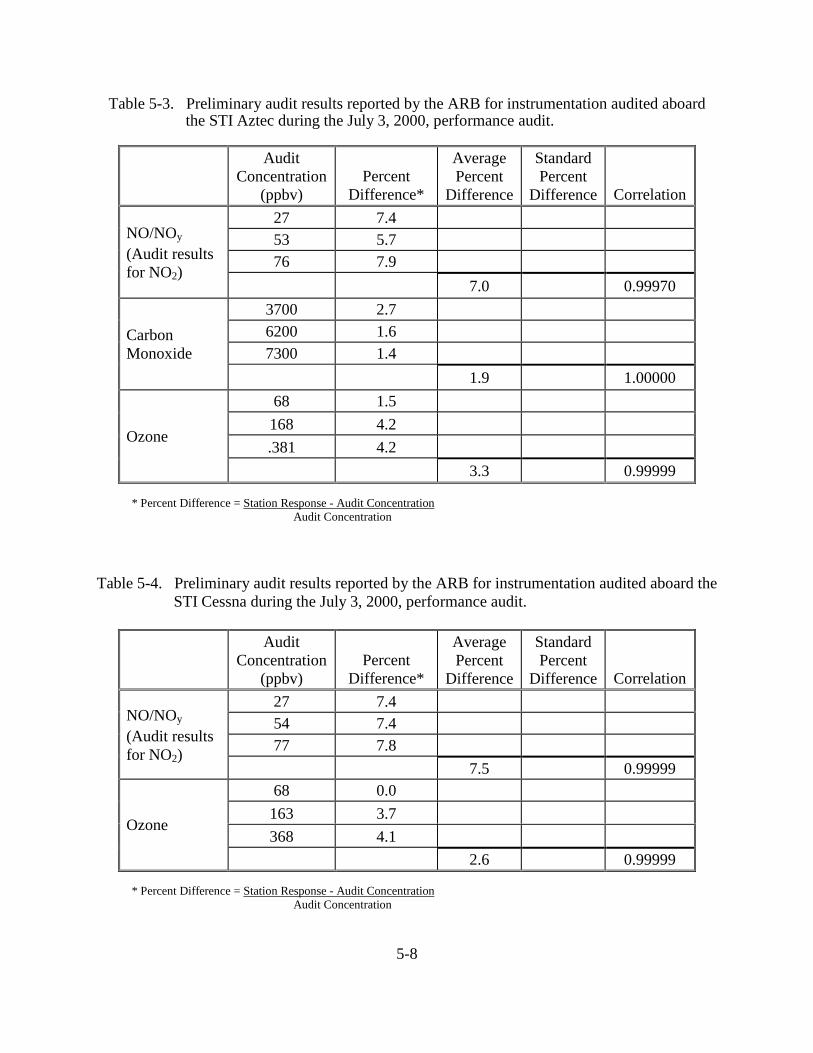
5-8
Table 5-3. Preliminary audit results reported by the ARB for instrumentation audited aboardthe STI Aztec during the July 3, 2000, performance audit.
AuditConcentration
(ppbv)Percent
Difference*
AveragePercent
Difference
StandardPercent
Difference Correlation27 7.453 5.776 7.9
NO/NOy
(Audit resultsfor NO2)
7.0 0.999703700 2.76200 1.67300 1.4
CarbonMonoxide
1.9 1.0000068 1.5168 4.2.381 4.2
Ozone
3.3 0.99999
* Percent Difference = Station Response - Audit ConcentrationAudit Concentration
Table 5-4. Preliminary audit results reported by the ARB for instrumentation audited aboard theSTI Cessna during the July 3, 2000, performance audit.
AuditConcentration
(ppbv)Percent
Difference*
AveragePercent
Difference
StandardPercent
Difference Correlation27 7.454 7.477 7.8
NO/NOy
(Audit resultsfor NO2)
7.5 0.9999968 0.0163 3.7368 4.1
Ozone
2.6 0.99999
* Percent Difference = Station Response - Audit ConcentrationAudit Concentration
5-9
5.3 RESULTS OF THE INTERCOMPARISON FLIGHTS
Two intercomparison flights were performed. On July 5, 2000, the STI Aztec flew anintercomparison with the DOE G-1 near Fresno. On July 6, 2000, both STI aircraft flew anintercomparison flight with the UCD Cessna 182 around Sacramento. For the comparison withthe DOE G-1 a flight route was agreed upon by the crews of both aircraft, including a series oftraverses and vertical profiles, and was executed separately. This was necessary because of asignificant disparity in speed between the two aircraft. The data collected aboard the Aztec forthat flight was submitted to Mr. David Bush.
For the comparison between the two STI aircraft and the UCD aircraft, a flight route,including several traverses and a vertical profile, was executed; all three aircraft flew in aformation with the STI Aztec in the lead, followed by the STI Cessna and the UCD Cessna,respectively. Data from that intercomparison were shared between the participants and weresubmitted to Mr. David Bush. The ozone, NO, and NOy measurements made aboard the threeaircraft all agreed to within the stated uncertainties for the different instruments. Thenephelometer mounted on the STI Cessna was not operational for the intercomparison flight.The results from the STI Aztec bscat measurement and the UCD Cessna bsp measurements agreedwell once the difference of Rayleigh scattering (measured with the Aztec instrument[~ 11 Mm-1]) was accounted for. Figures 5-1 through 5-3 show the time series data collectedaboard the STI aircraft during the July 6, 2000, intercomparison. The times were adjustedslightly to account for the distance between the aircraft.
5.4 COMPARISON OF AIRCRAFT, SURFACE, AND UPPER-AIR OBSERVATIONS
During the data validation process the measurements collected aboard both the STI Aztecand Cessna 182 were compared to several ground-based and wind profiler data sets. For theAztec, wind profilers located at Bodega Bay and Tracy were used to check the windmeasurements collected with the aircraft-mounted AIMMS-10 system. Ozone measurementsmade aboard the Aztec were checked against measurements made at the surface at Bethel Islandand Parlier. The Cessna 182 measurements for wind speed and direction, NO, NOy, ozone, andbsp were checked against the measurements made at the Angiola field site. In all cases the aloftand surface-based measurements showed good agreement for afternoon, well mixedobservations.
5.5 DESCRIPTION OF DATA COMPLETENESS, PRECISION, ACCURACY, ANDLOWER QUANTIFIABLE LIMIT
This section is currently under preparation and will be forwarded to ARB on or beforeDecember 19, 2001.
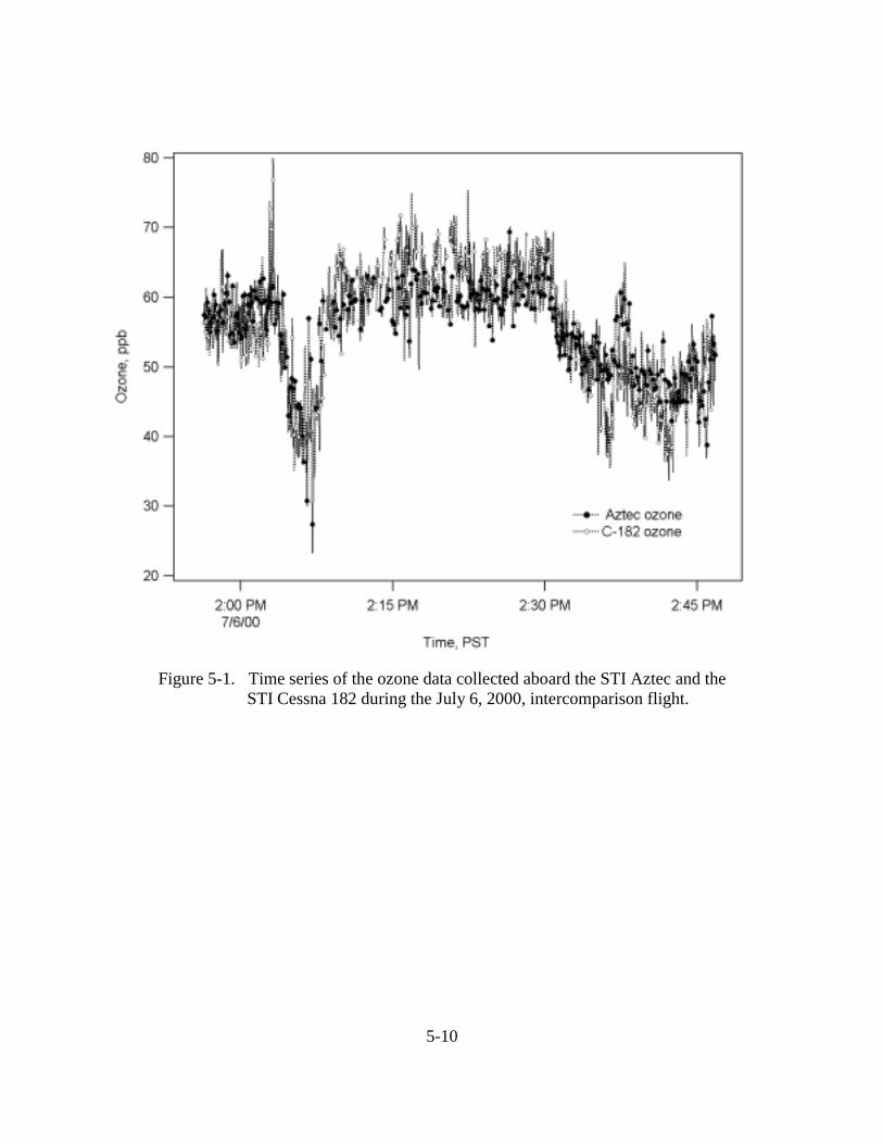
5-10
Figure 5-1. Time series of the ozone data collected aboard the STI Aztec and theSTI Cessna 182 during the July 6, 2000, intercomparison flight.
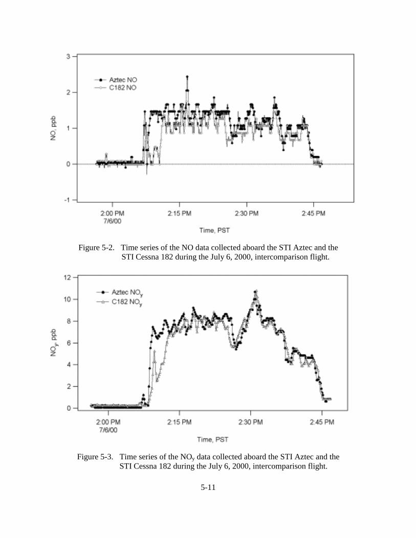
5-11
Figure 5-2. Time series of the NO data collected aboard the STI Aztec and the STI Cessna 182 during the July 6, 2000, intercomparison flight.
Figure 5-3. Time series of the NOy data collected aboard the STI Aztec and theSTI Cessna 182 during the July 6, 2000, intercomparison flight.
6-1
6. RESULTS AND RECOMMENDATIONS
The air composition and meteorology observations made with the STI aircraft duringCCOS comprise a useful database for further exploration of transport and chemical processes inthe SJV and upwind regions. The greatest utility of the Aztec data may be in establishing limitson the upwind boundary conditions. The observations made with the Cessna will be useful inexploration of the transport processes and chemical evolution attendant to ozone episodes in theSJV.
Highlights of the observations made with the Aztec include
• High quality data for ozone, NO, NOy, CO, bscat, and winds collected offshore at altitudesfrom 500-5000 ft. under a variety of conditions.
• Persistent layers of ozone concentration greater than 50 ppbv in air masses coming fromthe Pacific Ocean.
• Significant transport of pollutants from onshore sources to points 100 miles offshore.Preliminary evaluation of the air composition in these polluted layers suggest a forest firesource.
Highlights of the observations made with the Cessna include
• Excellent temporal and spatial coverage of the southern SJV during the two principalozone episodes experienced during summer 2000.
• Good spatial and chemical characterization of the Fresno and Bakersfield urban plumesand their transport to the greater valley.
• Multi-day repetitive flight patterns that will allow exploration of the physical andchemical conditions associated with SJV-wide ozone episodes.
In addition to providing a database useful for model evaluation, these observations couldbe used to investigate a number of specific topics:
• Compare and contrast ozone distribution and ozone production efficiency at the surfaceand aloft for the Bakersfield, Fresno, and Angiola field sites.
• Examine rural ozone in the SJV with respect to sources of precursors, dynamics, andlocal production versus advection
• Contribution of forest fires to SJV ozone and particulate matter.
7-1
7. REFERENCES
Buhr M.P., Alcorn S.H, and Blumenthal D.L. (2001) Central California Ozone Study AircraftData. Report prepared for the California Air Resources Board, Sacramento, CA bySonoma Technology, Inc., Petaluma, CA, STI-900106-2074-DV, August.
California Air Resources Board (2001) Central California Air Quality Study Data TransmittalFormat Document for CCOS. Release: CCOS021401A, February 14. Available at<http://www.arb.ca.gov/airways/CRPAQS/lookups.htm>.