Embed Size (px)
Citation preview
1
CALCULATION OF EXPECTED SLIDING DISTANCE OF
BREAKWATER CAISSON CONSIDERING VARIABILITY IN WAVE
DIRECTION
SU YOUNG HONG
School of Civil, Urban, and Geosystem Engineering, Seoul National University, San 56-1, Shinlim-Dong,
Gwanak-Gu, Seoul 151-742, Korea, E-mail: [email protected]
KYUNG-DUCK SUH1
School of Civil, Urban, and Geosystem Engineering & Research Institute of Marine Systems Engineering,
Seoul National University, San 56-1, Shinlim-Dong, Gwanak-Gu, Seoul 151-742, Korea, E-mail:
HYUCK-MIN KWEON
Department of Civil Engineering, Kyongju University, San 42-1, Hyohyun-Dong, Kyongju-Si,
Kyongsangbuk-Do 780-210, Korea, E-mail: [email protected]
1 Corresponding author, Temporal address until January, 2004: Department of Civil, Construction, and
Environmental Engineering, Oregon State University, 202 Apperson Hall, Corvallis, Oregon 97331-2302,
USA, Phone: +1-541-737-6891, Fax: +1-541-737-3052, Email: [email protected] or [email protected]
2
ABSTRACT
In this study, the reliability design method developed by Shimosako and Takahashi in
2000 for calculation of the expected sliding distance of the caisson of a vertical
breakwater is extended to take into account the variability in wave direction. The effects
of directional spreading and the variation of deepwater principal wave direction about its
design value were found to be minor compared with those of the obliquity of the
deepwater design principal wave direction from the shore-normal direction. Reducing the
significant wave height at the design site by 6% to correct the effect of wave refraction
when using Goda’s model was found to be appropriate when the deepwater design
principal wave direction was about 20 degrees. When we used the field data in a part of
the east coast of Korea, taking the variability in wave direction into account reduced the
expected sliding distance to about one third of that calculated without taking the
variability in wave direction into account, and the required caisson width was reduced by
about 10 % at the maximum.
Keywords: Breakwater; caisson; expected sliding distance; reliability design; variability
in wave direction; wave transformation model.
3
1. Introduction
In the conventional design of the caisson of a vertical breakwater, the required sizes of
the caisson are calculated from empirical formulas, with a certain margin of safety, so as
to resist the design load related to a given return period. The conventional method is
based on the force balance between the wave loads and the resistance of the caisson, and
no movement of the caisson is allowed. Any small movement of the caisson is
considered to be damage. However, even if the caisson moves, the breakwater can still
perform its function, unless the movement is so great as to stop the serviceability of the
breakwater. Therefore, if we allow a certain amount of movement of the caisson, a more
economical design could be made.
In the conventional design, it is assumed that the lifetime of a breakwater is the
same as the return period of the design wave. In this case, the probability of occurrence
of wave heights greater than the design wave height during the lifetime of the breakwater
is about 63 percent, which is larger than the probability for a wave height greater than the
design height not to occur. For the breakwater located outside surf zone, the maximum
wave height is usually taken to be 1.8 times the significant wave height, but a higher
wave could appear especially when the storm duration is long. Moreover, errors are
always involved in the computation of wave transformation and wave forces so that the
computed values could happen to be on the safe side. Considering all these uncertainties,
the conventional design uses a safety factor of 1.2 for sliding of a caisson, but its
reasoning is not so clear. If the design conditions are different inside and outside surf
zone, the degree of stability of the breakwater should not be the same, even if we use the
same safety factor.
In order to cope with the problems mentioned above, reliability design methods or
performance design methods have been developed, which take into account the
uncertainties of various design parameters and allow a certain amount of damage during
the lifetime of a breakwater. The reliability or performance design methods have been
developed since the mid-1980s, especially in Europe and Japan. In Europe, van der Meer
(1988) presented a probabilistic approach for the design of breakwater armor layer, and
Burcharth (1991) introduced partial safety factors in the reliability design of rubble
mound breakwaters. Recently Burcharth and Sørensen (1999) established partial safety
factor systems for rubble mound breakwaters and vertical breakwaters by summarizing
4
the results of the PIANC (Permanent International Association of Navigation
Congresses) Working Groups. The European reliability design methods belong to what is
called as Level 1 or Level 2 method. On the other hand, in Japan, Level 3 methods have
been developed, in which the expected damage of breakwater armor blocks (Hanzawa et
al., 1996) or the expected sliding distance of a breakwater caisson (Shimosako and
Takahashi, 2000; Goda and Takagi, 2000; Takayama et al., 2000) during its lifetime is
estimated. Monte Carlo simulations are used to take into account the uncertainties of
various design factors.
Among the above-mentioned Japanese authors, Hanzawa et al. (1996) and Goda
and Takagi (2000) used Goda's (1975) model to calculate the wave transformation from
deep water to the design site, which includes wave attenuation due to random breaking.
Unidirectional random waves normally incident to a straight coast with parallel depth
contours were assumed so that no wave refraction was involved. Shimosako and
Takahashi (2000) postulated wave transformation including refraction as well as shoaling
and breaking, but they also used Goda’s (1975) model in the actual computation
(Shimosako, 2003). In real situations, directional random waves with variable principal
wave directions will be incident to the shore. For more accurate computation of the wave
heights at the design site, therefore, we should use more realistic wave transformation
models taking into account the variability in wave direction. Recently Suh et al. (2002)
extended the method of Hanzawa et al. (1996) to include the effect of the variability in
wave direction in the calculation of the expected damage of breakwater armor blocks.
In the present study, by closely following Suh et al.’s (2002) approach, we extend the
reliability design method of Shimosako and Takahashi (2000) for calculation of the
expected sliding distance of the caisson of a vertical breakwater to take into account the
variability in wave direction. The variability in wave direction includes directional
spreading of random directional waves, obliquity of the design principal wave direction
from the shore-normal direction, and its variation about the design value. To calculate the
transformation of random directional waves over an arbitrary bathymetry including surf
zone, we used Kweon et al.’s (1997) model, which was also used by Suh et al. (2002).
In the following section, the mathematical model to calculate the sliding distance of
a caisson is described. In Sec. 3, the computational procedure for calculating the
expected sliding distance of a caisson is explained. In Sec. 4, several computational
examples are presented to compare the results of the present study with those of previous
5
authors and to illustrate the importance of wave directionality. The major conclusions
then follow.
2. Computation of Sliding Distance
The distance of caisson sliding is calculated with the model presented by Shimosako and
Takahashi (2000), which is summarized below for the sake of completeness. Assuming
that the caisson sliding is small enough to neglect the wave-making resistance force
behind the caisson, the equation of motion describing caisson sliding is given by
RG
a FPdt
xdM
g
W
2
2
(1)
where W is the caisson weight in the air, g the gravity, aM the added mass
( 20 '0855.1 h ), 0 the density of sea water, 'h the water depth from bottom of
caisson to design water level, Gx the horizontal displacement of caisson, P the
horizontal wave force, RF the frictional resistance force UW ' , the friction
coefficient, 'W the caisson weight in water, and U the uplift force. The sliding
distance of the caisson can be calculated by numerically integrating the preceding
equation twice with respect to time.
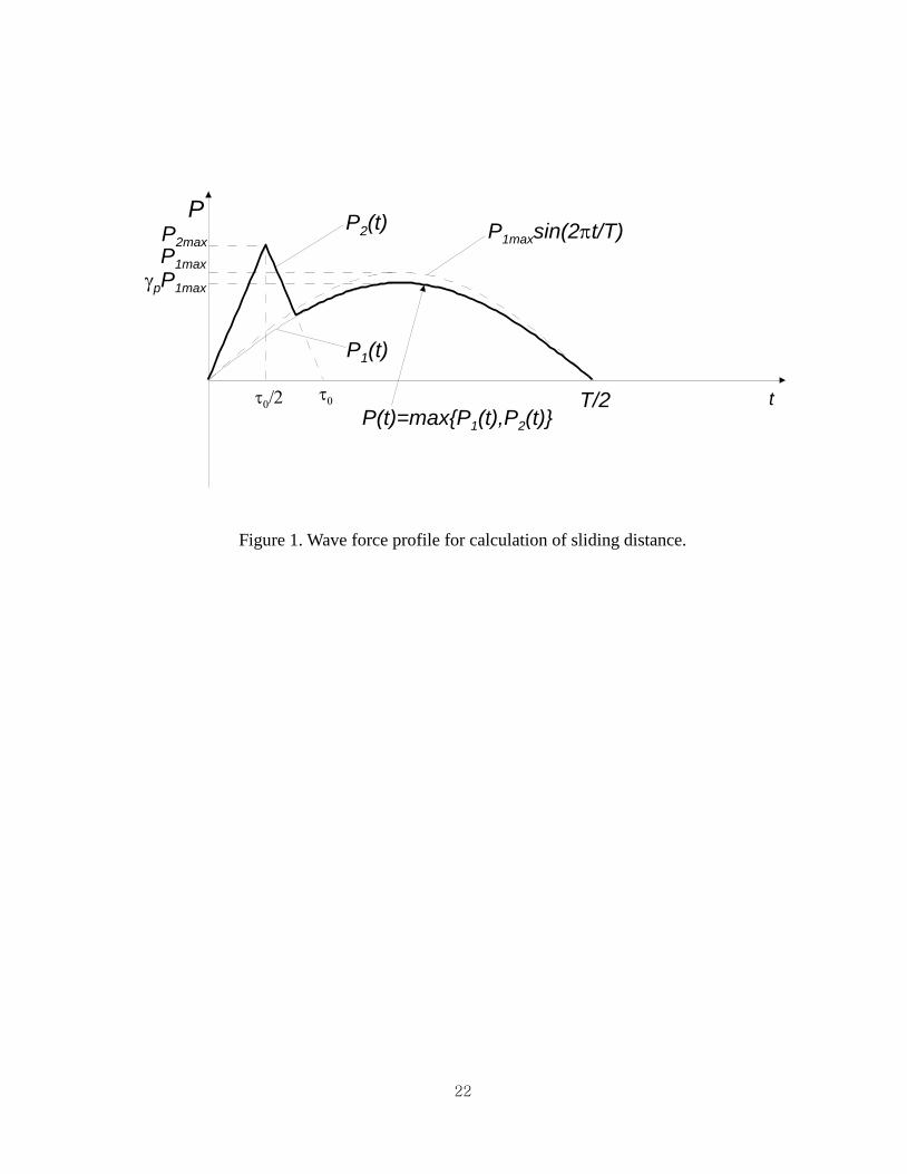
The horizontal force )(tP is calculated by taking the larger value of a sinusoidal
form tP1 representing standing wave pressures and a triangular pulse tP2
indicating impulsive pressures as shown in Figure 1, i.e.,
tPtPtP 21 ,m a x (2)
tP1 and tP2 are defined as follows:
T
tPtP P
2sinmax11 (3)
6
0
00
max20
0max2
0
2
,0
2,12
20,
2
t
tPt
tPt
tP (4)
02
sin:2
sin1 max12max12max1
2
1
T
tPtPdt
T
tPtP
TP
t
tP
(5)
where the time interval 21 ,tt indicates the interval satisfying
0)/2sin()( max12 TtPtP , max1P the horizontal wave force calculated by the
Goda (1974) pressure formula considering only the parameter 1 , max2P the wave
force calculated by using the Takahashi et al.'s (1994) parameter * in place of 2 in
the Goda formula, T the wave period, and 0 the duration of the impulsive wave
force. The parameter P is used to reduce the sinusoidally varying standing wave force
by the amount increased due to the impulsive force.
Similarly, tU is calculated as follows:
tUtUtU 21 ,max (6)
T
tUtU U
2sinmax1 (7)
7
0
00
max0
0max
0
2
,0
2,12
20,
2
t
tUt
tUt
tU (8)
02
sin:2
sin1 max2max2max
2
1
T
tUtUdt
T
tUtU
TU
t
tU
(9)
where maxU denotes the uplift force calculated from the Goda formula.
The term 0 is related to the wave period as follows:
Fk 00 (10)
where the time F0 and the constant k are given by
8.0,4.0
8.00,8
5.0
0
h
HT
h
HT
h
H
F (11)
and
2
3.0* 1
1
k (12)
respectively. Here H is the wave height, and h the water depth.
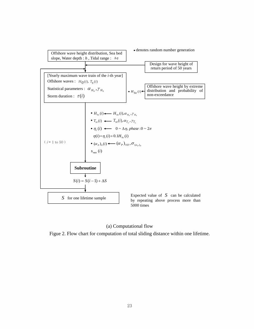
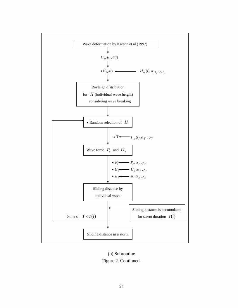
3. Procedure for Computation of Expected Sliding Distance
8
In this section, the procedure for computing the expected sliding distance is explained in
conjunction with the computational flow chart sketched in Figure 2. In general, the
sliding of a breakwater caisson is caused by large waves comparable to the design waves.
Therefore, the annual maximum wave height is considered sufficient to be incorporated
into the calculation. The annual maximum offshore significant wave height eH0 is
randomly sampled from the extreme wave height distribution (Weibull distribution in
this study), and the peak of storm waves is assumed to continue for 2 hours. This wave
height is further given a stochastic variation with the normal distribution having a mean
0H and standard deviation 0H
. This variation represents the uncertainty in the
estimate of the extreme distribution function owing to the limited sample size of extreme
wave data or the inaccuracy in wave hindcasts. The mean and standard deviation are
assumed to have the following relations with eH0 (Takayama and Ikeda, 1994):
eHH H0)1(00
, eHH H000 (13)
where 0H
and 0H
denote the bias and deviation coefficient, respectively. The
sample offshore wave height cH0 to be employed in the calculation is then determined
by a normalized random number based on Eq. (13). The corresponding significant wave
period is determined to yield a constant wave steepness (0.03 in this study) in the
offshore area:
g
HT cse
03.0
2 0 (14)
This wave period may also contain uncertainty and thus is given a stochastic variation
with the normal distribution having a mean sT and standard deviation
sT . The mean
and standard deviation are assumed to have the following relations with seT :
9
seTT Tss)1( , seTT T
ss (15)
where sT
and sT
denote the bias and deviation coefficient, respectively. The sample
significant wave period scT to be employed in the calculation is then determined by a
normalized random number based on Eq. (15).
Offshore random directional waves with the directional spreading parameter maxs
are assumed to be incident with the principal wave direction 0P counterclockwise
with respect to the shore-normal direction. The principal wave direction is assumed to
have a stochastic variation with the normal distribution having a mean being the same as
the design principal wave direction DP 0 and a standard deviation 0p
.
Unidirectional random waves normally incident to the shore are simulated by setting
maxs , 00
p , and 0
0
Dp . The offshore directional wave spectrum was
expressed as the product of the Bretschneider-Mitsuyasu frequency spectrum and the
Mitsuyasu-type directional spreading function (Goda, 2000, Section 2.3.2).
With the tidal range of , tide level t was assumed to vary sinusoidally
between LWL( 0t ) and HWL( t ). The effect of storm surge was taken into
account by adding %10 of the deepwater wave height to the tide level.
Once the offshore wave height, wave period, and tide level are determined, the
significant wave height at the location of the breakwater should be calculated. In order to
take into account the effect of wave direction on wave transformation, we use Kweon et
al.’s (1997) wave transformation model in the present study. The significant wave height
at the design site seH , calculated by the wave transformation model, is also assumed to
have computational uncertainty, and thus is given stochastic variation with the normal
distribution as with the offshore wave height. The mean sH and the standard deviation
sH are assumed to have the following relations with seH :
10
seHH Hss)1( , seHH H
ss (16)
where sH
and sH
denote the bias and deviation coefficient, respectively. The
sample wave height at the design site scH is determined by a normalized random
number based on Eq. (16). The Kweon et al.’s (1997) model computes the mean wave
direction as well as the wave height at the design site. The computed wave direction is
used as an input parameter in the calculation of wave pressure using the Goda formula.
Once the significant wave height at the location of the breakwater is calculated, the
heights of the individual waves during the storm are randomly sampled by assuming the
Rayleigh distribution. An individual wave height greater than the breaking wave height
was reduced to the breaking wave height using the formula in Goda (2000, p. 81). The
periods of the individual waves are given stochastic variation with the normal
distribution as with the significant wave period. The mean T and the standard
deviation T are assumed to have the following relations with scT :
scTT T)1( , scTT T (17)
where T and T denote the bias and deviation coefficient, respectively.
Theoretically, the total sliding distance during the lifetime of a breakwater should
be calculated by summing the sliding distances due to all the high waves during the
lifetime. In the present study, however, we assume that the waves high enough to make a
caisson slide appear once a year so that the annual maximum wave height is sufficient to
be incorporated into the calculation. Therefore, the total sliding distance is obtained by
repeating the calculation for the number of years of the breakwater lifetime (usually 50
years). The process of one lifetime cycle is shown in Figure 2. This process is repeated a
large number of times, and the expected sliding distance is obtained by taking the
average of the total sliding distance during each lifetime cycle. In order to take into
account the stochastic variation of various design parameters such as wave height, wave
period, water level, wave force, and friction coefficient, the Monte-Carlo simulation
11
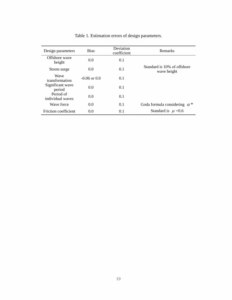
method was used. Table 1 lists the design parameters employed in the present study and
their bias and deviation coefficient.
4. Illustrative Examples
In this section, we present several computational examples to compare our results with
those of previous authors and to illustrate the importance of wave directionality. We
consider only a plane beach, which is simple but sufficient to illustrate the influence of
wave directionality. The common computational conditions are given below.
The Weibull distribution function with the shape parameter 0.2k , scale parameter
23.2A , and location parameter 78.4B was used as the extreme distribution of the
offshore wave height, which gave a design deepwater wave height with a return period of
50 years to be 9.2 m. The deepwater wave steepness was assumed to be constant at 03.0
so that the corresponding design wave period was 0.14 s. The bias and deviation
coefficient of various design parameters are given in Table 1, which are basically the
same as those used by Shimosako and Takahashi (2000). In the surf zone, the deviation
coefficient of wave force of obliquely incident waves may be smaller than that of normal
incidence, because the impulsive breaking wave pressure with larger deviation than
standing wave pressure occurs only when the wave direction is almost normal to the
breakwater. Unfortunately, however, there is not enough experimental data about this.
Therefore, we used the same value as that used by Shimosako and Takahashi (2000)
regardless of wave direction, because their results are later compared with the present
model results. A tidal range of 2.0 m was assumed, and water depths from 10 to 30 m at
LWL at an interval of 2 m were examined. Seabed slopes of 1/50 and 1/20 were used.
The design wave height at each water depth was determined by computing the wave
heights corresponding to 2.90 H m while changing the water level from LWL to
HWL and taking the largest wave height. The total number of simulations for the
calculation of expected sliding distance was chosen to be 5000 based on Shimosako
and Takahashi (2000), who have shown that a stable statistical result can be obtained by
doing so.
The breakwater is assumed to be installed parallel to the shoreline. The design
significant wave heights, maximum wave heights and caisson widths at different water
12
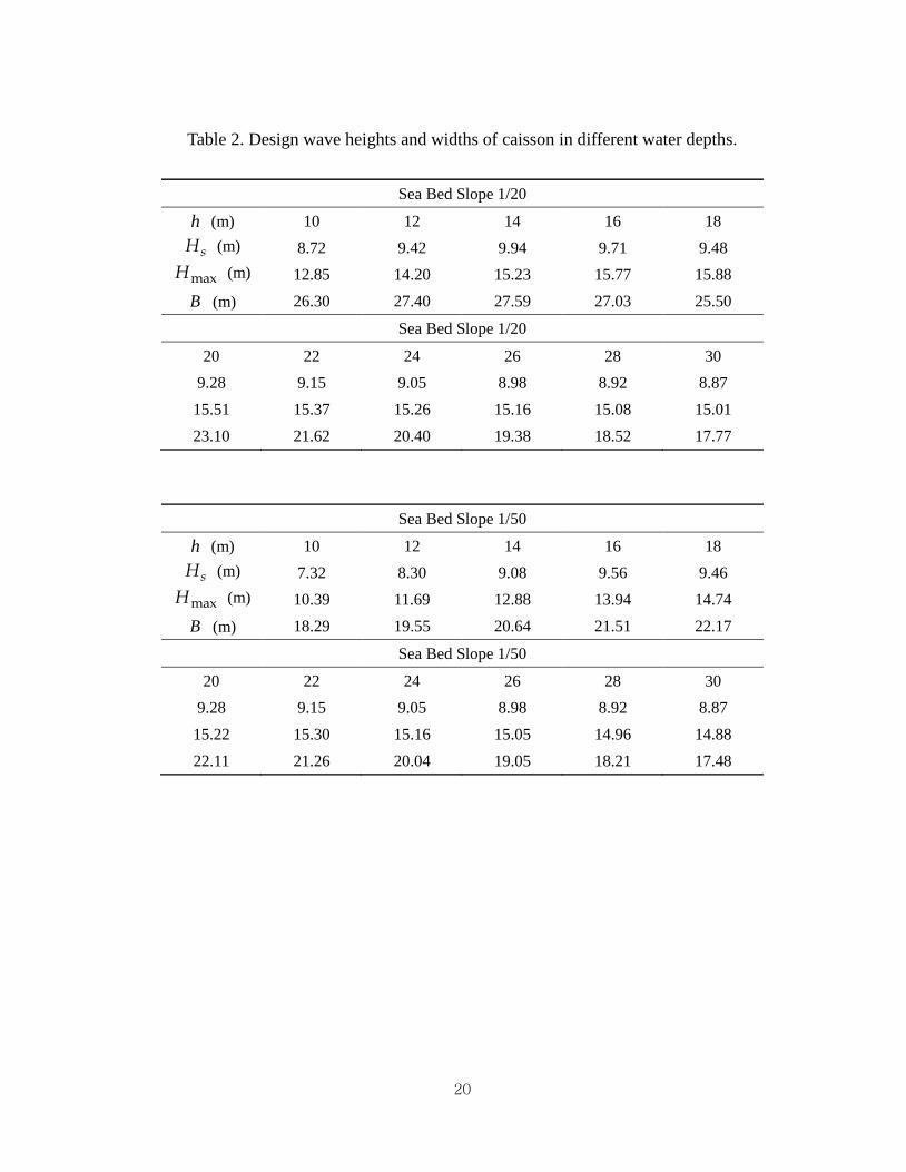
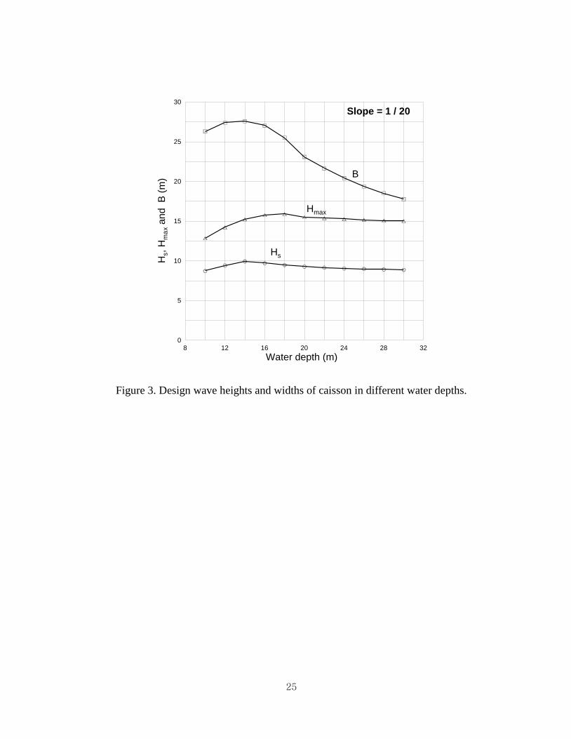
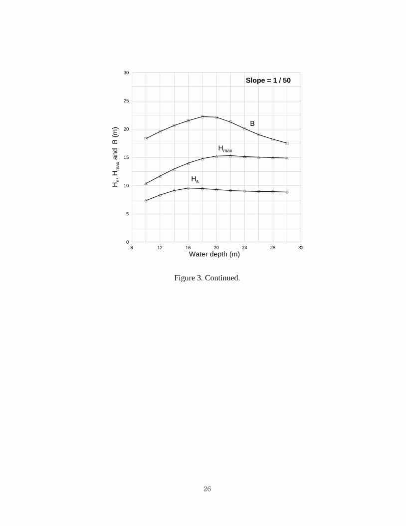
depths are given in Table 2. These values are also plotted in Figure 3 for later use. A
constant mound berm width of 8 .0 m was used regardless of water depth. The crest
elevation of the caisson was taken to be 6.0 times the design significant wave height at
the location of the breakwater. The water depth on the rubble mound, d , was taken to be
h65.0 . The height from the bottom of the caisson to the top of the rubble mound was assumed to
be 2.0 m so that 0.2' dh m was used. The width of the caisson was calculated by the
Goda formula with the safety factor of 2.1 . In the following, the expected sliding
distance was calculated for the caisson width given in Table 2 in each water depth.
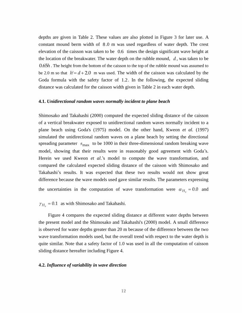
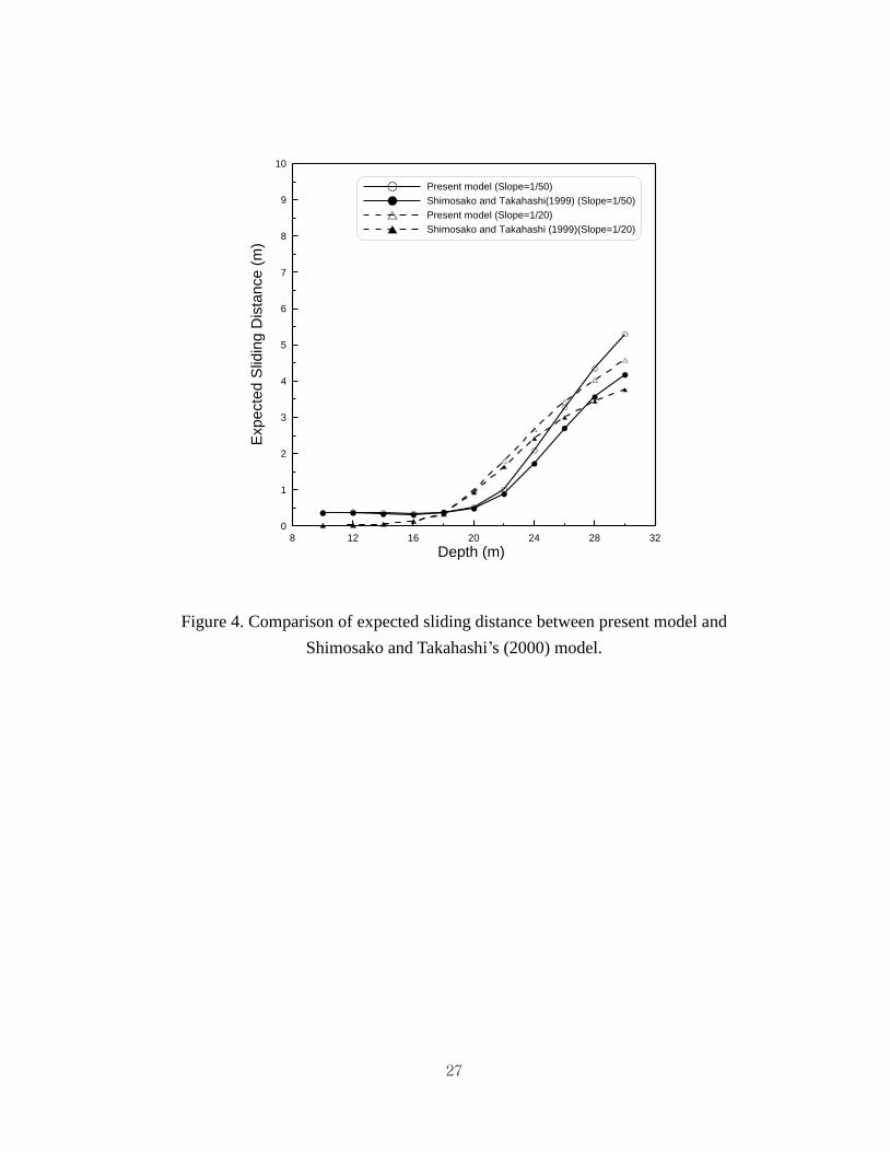
4.1. Unidirectional random waves normally incident to plane beach
Shimosako and Takahashi (2000) computed the expected sliding distance of the caisson
of a vertical breakwater exposed to unidirectional random waves normally incident to a
plane beach using Goda's (1975) model. On the other hand, Kweon et al. (1997)
simulated the unidirectional random waves on a plane beach by setting the directional
spreading parameter maxs to be 1000 in their three-dimensional random breaking wave
model, showing that their results were in reasonably good agreement with Goda’s.
Herein we used Kweon et al.’s model to compute the wave transformation, and
compared the calculated expected sliding distance of the caisson with Shimosako and
Takahashi’s results. It was expected that these two results would not show great
difference because the wave models used gave similar results. The parameters expressing
the uncertainties in the computation of wave transformation were 0.0sH
and
1.0sH
as with Shimosako and Takahashi.
Figure 4 compares the expected sliding distance at different water depths between
the present model and the Shimosako and Takahashi's (2000) model. A small difference
is observed for water depths greater than 20 m because of the difference between the two
wave transformation models used, but the overall trend with respect to the water depth is
quite similar. Note that a safety factor of 1.0 was used in all the computation of caisson
sliding distance hereafter including Figure 4.
4.2. Influence of variability in wave direction
13
The primary purpose of the present study is to examine the influence of the variability in
wave direction upon the computation of the expected sliding distance of a caisson, which
was not included in Goda's (1975) model. For this purpose, we carried out the
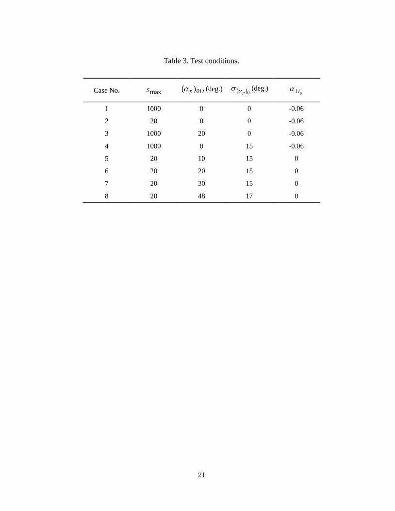
computation for the eight cases listed in Table 3.
Case 1 is for unidirectional waves normally incident to the beach as in Goda's (1975)
model. Case 2 includes the effect of directional spreading. The spreading parameter
maxs equal to 20 was used, which corresponds to the deepwater wave steepness of 0.03
(Goda, 2000, p. 35). Case 3 is for unidirectional waves incident at 20 with respect to the
shore-normal direction, including only the effect of wave refraction. Case 4 examines the
effect of the variation of the principal wave direction. 0)( 0 Dp and 150)(
p
were used. For Cases 1 to 4, 06.0sH
and 1.0sH
were used. Cases 2 to 4,
however, included a fraction of the effects of refraction and directional spreading that
were ignored in Goda’s (1975) model. Therefore, the bias must be smaller than –0.06,
e.g., –0.04. However, how small was uncertain, so the value of –0.06 was used without
change. Cases 5 to 8 included all of the variability in wave direction partly considered in
Cases 2 to 4. To examine the influence of the principal wave direction, the expected
sliding distance was calculated in Cases 5 to 7 with the deepwater principal wave
direction of 10, 20, and 30 degrees, respectively. Case 8 represented the typical
conditions between Uljin and Pohang in the east coast of Korea as given by Suh et al.
(2002). In Cases 5 to 8, all of the variability in wave direction was included, so no bias
was assumed in the computation of wave transformation, i.e., 0.0sH
was used.
However, the computational error must still exist, so 1.0sH
was kept the same.
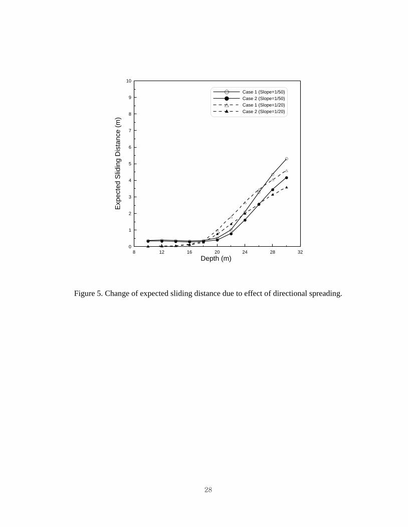
Figure 5 shows a comparison of the expected sliding distance at different water
depths between Case 1 and 2. In Case 2 where the effect of directional spreading is
included, the wave height at the location of the breakwater becomes smaller compared
with that of the unidirectional waves in Case 1. Therefore, the expected sliding distance
in Case 2 is smaller than in Case 1. The difference of expected sliding distance between
the two cases becomes smaller as water depth decreases, because the effect of directional
14
spreading disappears as the waves propagate toward the shore.
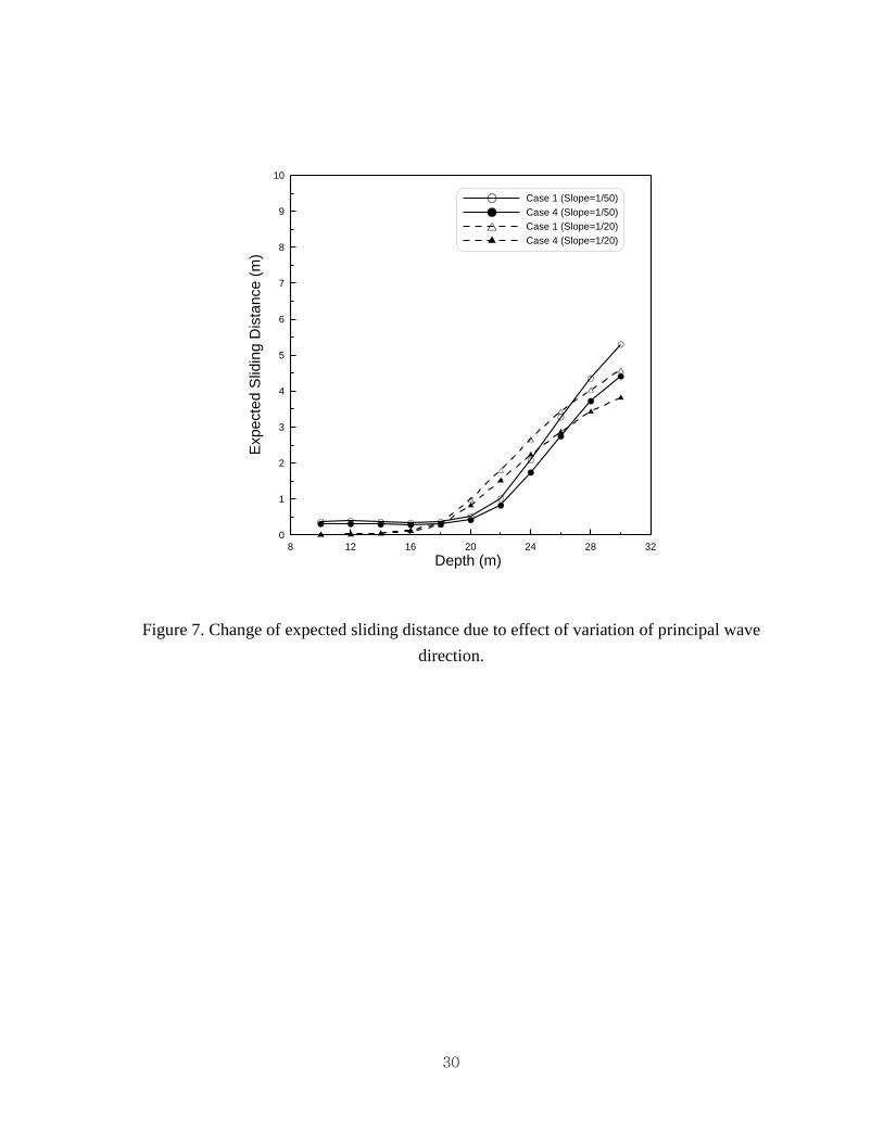
Figure 6 shows a comparison between Case 1 and 3. The height of obliquely
incident waves is smaller than that of normally incident waves owing to wave refraction.
Thus, the expected sliding distance in Case 3 is smaller than in Case 1. Figure 7 shows a
comparison between Case 1 and 4. Again due to the effect of wave refraction, the
expected sliding distance in Case 4 is computed to be smaller than in Case 1. Figure 6
and 7 show that the effect of wave refraction diminishes with decreasing water depth.
This is probably because, in shallow water, the maximum wave height is restricted by the
water depth so that the wave thrust has an upper limit.
Comparison of Figures 5 to 7 shows that the effect of directional spreading is
almost same as that of variation of principal wave direction, but the effect of wave
refraction is greater than these two effects even for a relatively small deepwater wave
incident angle of 20 degrees.
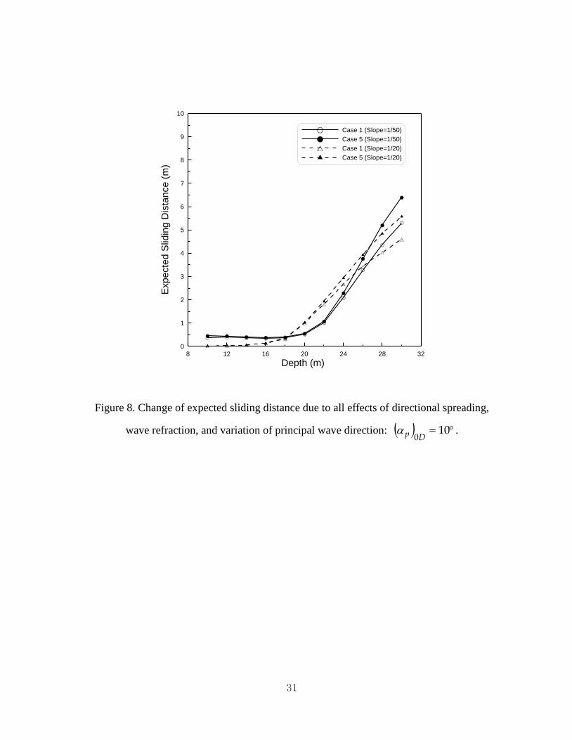
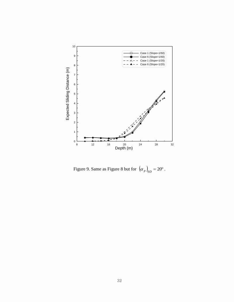
Figures 8, 9 and 10 show comparisons between Case 1 and Cases 5, 6 and 7,
respectively, which examine the influence of the principal wave direction on the
expected sliding distance when all the variability in wave direction is taken into account.
In Cases 5, 6 and 7, the deepwater principal wave direction was 10, 20 and 30 degrees,
respectively. As seen in Figure 8, when the deepwater principal wave direction was 10
degrees, the expected sliding distance calculated with the variability in wave direction
taken into account is greater than that calculated without taking the variability into
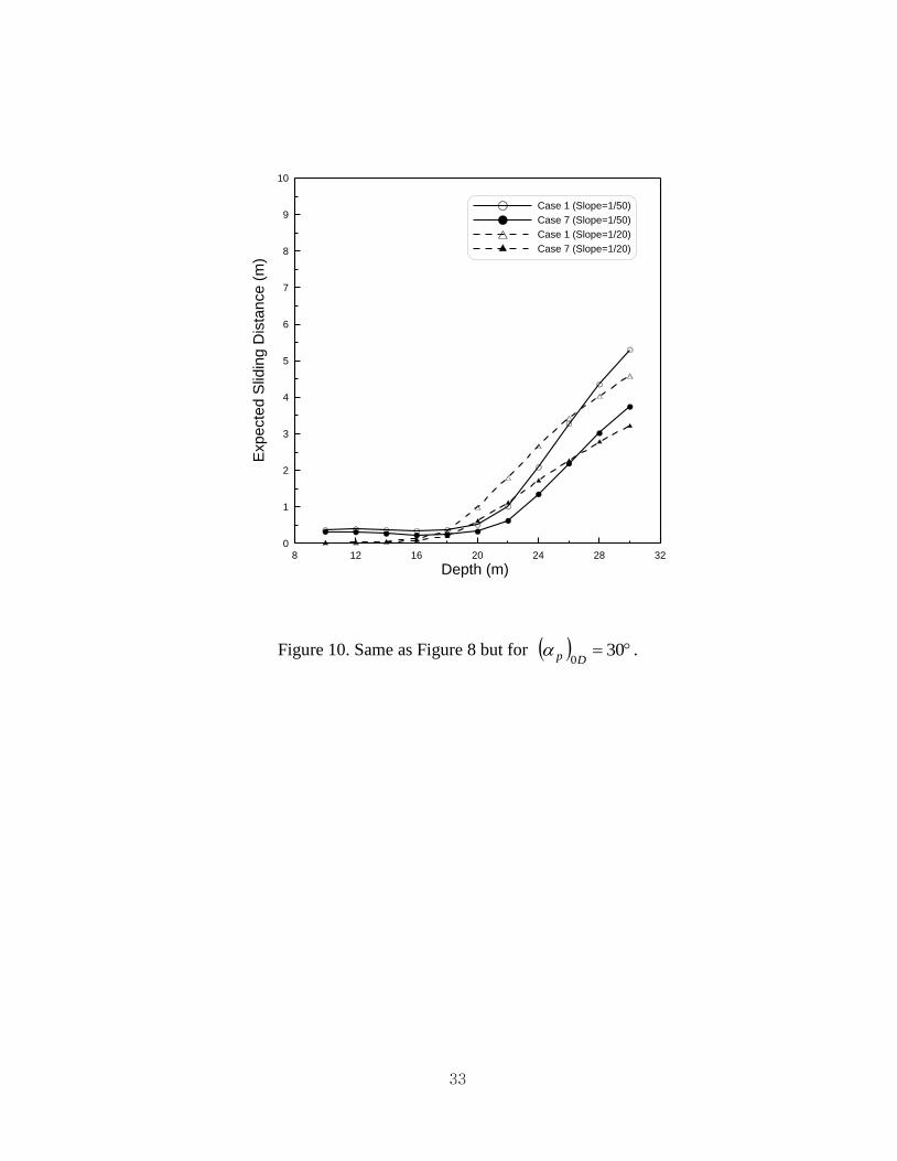
account. On the contrary, when the principal wave direction was 30 degrees, the opposite
occurs as shown in Figure 10. On the other hand, the expected sliding distances
calculated with and without taking the variability in wave direction into account almost
coincide each other when the principal wave direction was 20 degrees, as shown in
Figure 9. From the results given in Figures 8 to 10, we can say that the bias
06.0sH
employed to take into account the variability in wave direction is suitable
when the deepwater design principal wave direction is about 20 . Note that the bias
06.0sH
was used in Case 1 but 0.0sH in Cases 5 to 7. A value smaller than
06.0 in magnitude (e.g., 04.0 ) should be used when Dp 0
is smaller than 20 ,
or vice versa. More computations may be needed for different wave conditions and
15
seabed slopes to obtain a more reliable relation between Dp 0
and sH .
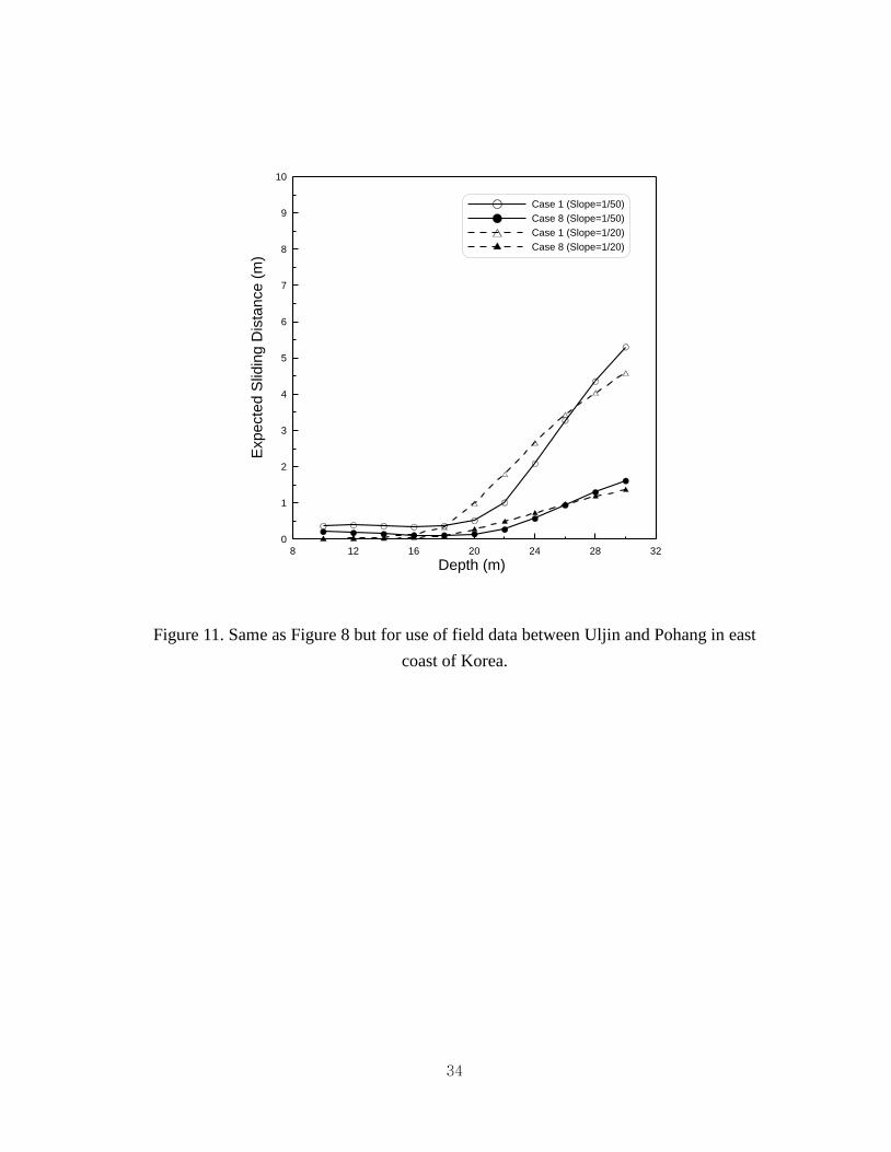
Figure 11 shows a comparison between Case 1 and 8. Because the deepwater
principal wave direction is very large at 48 in Case 8, the significant wave height at
the location of the breakwater is calculated to be very small due to the effect of severe
wave refraction. Therefore, the expected sliding distance in Case 8 is very small
compared with that in Case 1. The difference from Case 1 is prominent even in smaller
water depths, which is seen a little in Figure 10 but is hardly seen in Figures 8 and 9,
where the deepwater principal wave direction is relatively small and so is wave
refraction.
When the seabed slope is 1/20, the expected sliding distances are very small in
water depths smaller than about 16 m for all the cases shown in Figures 4 to 11. As
shown in Figure 3, the caisson width is quite large in these water depths of 1/20 beach
slope though maxH decreases with decreasing water depth because of wave breaking. It
seems that inside the surf zone of a steep beach the conventional design method is too
conservative in the viewpoint of expected sliding distance. Another feature seen in
Figures 4 to 11 is that the expected sliding distance of 1/20 slope is smaller than that of
1/50 slope in water depths smaller than about 18 m, the reverse happens in water depths
between 18 and 26 m, and the reverse happens again in greater water depths. This also
seems to be related to the caisson widths shown in Figure 3. On the beach of 1/20 slope
the caisson widths are relatively large in smaller water depths, while on the 1/50 slope
beach relatively large caisson widths are needed in the middle water depths of 16 to 22 m.
Again it seems that the conventional design method is conservative so that a smaller
expected sliding distance is calculated when the caisson width is relatively large.
However, the influence of seabed slope is not clear and further investigation is needed.
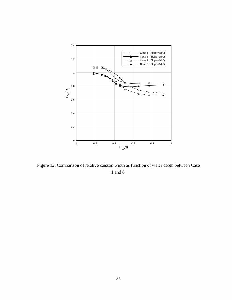
Figure 12 shows the ratio of 30B , the caisson width designed for the expected
sliding distance to be 30 cm, to dB , the caisson width designed with the conventional
method, as a function of water depth, for Cases 1 and 8. In this figure, the relative
caisson width dBB /30 smaller than 1.0 means that the present design method is more
economical than the conventional one, or vice versa. Even in Case 1 where the
variability in wave direction was not taken into account, the present design method is
more economical than the conventional one in water depths smaller than about 25 m (or
16
37.0/0 hH D ), while the reverse is true in deeper water. However, since hH D /0 is
larger than 0.37 for most ordinary design conditions, the present design method generally
gives a more economical cross section. In Case 8 where the variability in wave direction
was taken into account, dBB /30 is smaller than 1.0, indicating that the present design
method is more economical than the conventional one in all the water depths examined.
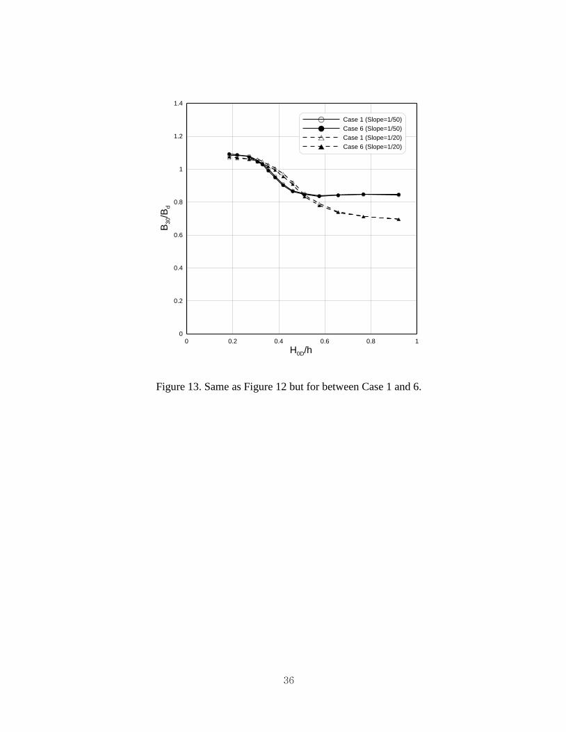
Other cases show similar trends except that the difference from Case 1 is different for
each case. For example, dBB /30 is almost same between Case 1 and 6 as shown in
Figure 13. Note that the expected sliding distance was almost same between these two
cases (see Figure 9).
5. Conclusions
In this study, the deformation-based reliability design method developed by Shimosako
and Takahashi (2000) for calculating the expected sliding distance of the caisson of a
vertical breakwater was extended to take into account the variability in wave direction.
On the whole, the effect of directional spreading or the variation of the deepwater
principal wave direction about its design value is not so significant, but the effect of the
obliquity of the design principal wave direction from the shore-normal direction is
relatively important so that the expected sliding distance tends to decrease with
increasing obliquity of principal wave direction. Especially in the case where the field
data in the east coast of Korea were used, the expected sliding distance calculated with
the variability in wave direction taken into account was reduced to about one third of that
calculated without taking the variability into account.
Reducing the significant wave height at the design site by 6 % to correct the effect
of wave refraction neglected by assuming unidirectional waves normally incident to a
coast with straight and parallel depth contours seems to be appropriate for the deepwater
design principal wave direction of about 20 degrees. A smaller or larger reduction should
be used for the deepwater principal wave direction smaller or larger, respectively, than 20
degrees. It may also be possible to propose a relationship between the deepwater design
principal wave direction and the bias of wave transformation through more computation
in the future.
If we design the caisson with the allowable expected sliding distance of 30 cm, in
17
water depths smaller than about 25 m, even without taking the variability in wave
direction into account, the width of the caisson could be reduced up to 30 percent
compared with the conventional design. When we used the field data in the east coast of
Korea and took into account the variability in wave direction, the required caisson width
was reduced by about 10 percent at the maximum, and a smaller caisson width was
required than the conventional design in the whole range of water depth (10 to 30 m).
Acknowledgement
This work was supported by the Brain Korea 21 Project.
References
Burcharth, H. F. (1991). “Introduction of partial coefficient in the design of rubble
mound breakwaters.” Proc. Conf. on Coastal Structures and Breakwaters, Inst. of
Civil Engrs., London, pp. 543-565.
Burcharth, H. F. and Sørensen, J. D. (1999). “The PIANC safety factor system for
breakwaters.” Proc. Int. Conf. Coastal Structures ’99, A. A. Balkema, Spain, pp.
1125-1144.
Goda, Y. (1974). “A new method of wave pressure calculation for the design of
composite breakwater.” Proc. 14th Int. Conf. on Coastal Engrg., American Soc. of
Civil Engrs., Copenhagen, pp. 1702-1720.
Goda, Y. (1975). “Irregular wave deformation in the surf zone.” Coastal Engrg., Japan,
18, pp. 13-26.
Goda, Y. (2000). Random Seas and Design of Maritime Structures, 2nd edn., World
Scientific, Singapore.
Goda, Y. and Takagi, H. (2000). “A reliability design method of caisson breakwaters
with optimal wave heights.” Coastal Engrg. J., 42(4), pp. 357-387.
Hanzawa, M., Sato, H., Takahashi, S., Shimosako, K., Takayama, T. and Tanimoto, K.
(1996). “New stability formula for wave-dissipating concrete blocks covering
horizontally composite breakwaters.” Proc. 25th Int. Conf. on Coastal Engrg.,
18
American Soc. of Civil Engrs., Orlando, pp. 1665-1678.
Kweon, H.-M., Sato, K. and Goda, Y. (1997). “A 3-D random breaking model for
directional spectral waves.” Proc. 3rd Int. Symp. on Ocean Wave Measurement and
Analysis, American Soc. of Civil Engrs., Norfolk, pp. 416-430.
Shimosako, K. (2003). Personal communication.
Shimosako, K. and Takahashi, S. (2000). “Application of deformation-based reliability
design for coastal structures.” Proc. Int. Conf. Coastal Structures ’99, A. A. Balkema,
Spain, pp. 363-371.
Suh, K. D., Kweon, H.-M. and Yoon, H. D. (2002). “Reliability design of breakwater
armor blocks considering wave direction in computation of wave transformation.”
Coastal Engrg. J., 44(4), pp. 321-341.
Takahashi, S., Tanimoto, K. and Shimosako, K. (1994). “A proposal of impulsive
pressure coefficient for the design of composite breakwaters.” Proc. Int. Conf. Hydro-
Technical Engrg. for Port and Harbour Constuction, Yokosuka, Japan, pp. 489-504.
Takayama, T. and Ikeda, N. (1994). “Estimation of encounter probability of sliding for
probabilistic design of breakwater.” Proc. Wave Barriers in Deepwaters, Port and
Harbour Research Institute, Yokosuka, pp. 438-457.
Takayama, T., Ikesue, S.-I. and Shimosako, K.-I. (2000). "Effect of directional
occurrence distribution of extreme waves on composite breakwater reliability in
sliding failure." Proc. 27th Int. Conf. on Coastal Engrg., American Soc. of Civil
Engrs., Sydney, pp. 1738-1750.
van der Meer, J. W. (1988). “Deterministic and probabilistic design of breakwater armor
layers.” J. Waterway, Port, Coastal and Ocean Engrg., American Soc. of Civil
Engrs., 114, pp. 66-80.
19
Table 1. Estimation errors of design parameters.
Design parameters Bias Deviation coefficient
Remarks
Offshore wave height
0.0 0.1
Storm surge 0.0 0.1 Standard is 10% of offshore
wave height Wave
transformation -0.06 or 0.0 0.1
Significant wave period
0.0 0.1
Period of individual waves
0.0 0.1
Wave force 0.0 0.1 Goda formula considering *
Friction coefficient 0.0 0.1 Standard is =0.6
20
Table 2. Design wave heights and widths of caisson in different water depths.
Sea Bed Slope 1/20
h (m) 10 12 14 16 18
sH (m) 8.72 9.42 9.94 9.71 9.48
maxH (m) 12.85 14.20 15.23 15.77 15.88
B (m) 26.30 27.40 27.59 27.03 25.50
Sea Bed Slope 1/20
20 22 24 26 28 30
9.28 9.15 9.05 8.98 8.92 8.87
15.51 15.37 15.26 15.16 15.08 15.01
23.10 21.62 20.40 19.38 18.52 17.77
Sea Bed Slope 1/50
h (m) 10 12 14 16 18
sH (m) 7.32 8.30 9.08 9.56 9.46
maxH (m) 10.39 11.69 12.88 13.94 14.74
B (m) 18.29 19.55 20.64 21.51 22.17
Sea Bed Slope 1/50
20 22 24 26 28 30
9.28 9.15 9.05 8.98 8.92 8.87
15.22 15.30 15.16 15.05 14.96 14.88
22.11 21.26 20.04 19.05 18.21 17.48
21
Table 3. Test conditions.
Case No. maxs Dp 0)( (deg.) 0)( p
(deg.) sH
1 1000 0 0 -0.06
2 20 0 0 -0.06
3 1000 20 0 -0.06
4 1000 0 15 -0.06
5 20 10 15 0
6 20 20 15 0
7 20 30 15 0
8 20 48 17 0
22
P
t
P2(t)
P1(t)
T/2
P1maxsin(2t/T)
P(t)=max{P1(t),P2(t)}
P2max
P1max
pP1max
Figure 1. Wave force profile for calculation of sliding distance.
23
)(0 iH e
)(0 iH c
00,),(0 HHe iH
)(iTsc ss TTse iT ,),(
)(it 2~0:,~0 phase
)(1.0)()( 0 iHii ct
)()( 0 iP 0)(0 ,)(
PDP
)(max is
SiSiS )1()(
(a) Computational flow
Figue 2. Flow chart for computation of total sliding distance within one lifetime.
Offshore wave height distribution, Sea bed
slope, Water depth : h , Tidal range :
[Yearly maximum wave train of the i-th year]
Offshore waves : )(),(0 iTiH s
Statistical parameters : 00
, HH
Storm duration : )(i
denotes random number generation
Design for wave height of return period of 50 years
Offshore wave height by extreme distribution and probability of non-exceedance
Subroutine
S for one lifetime sample
( i = 1 to 50 ) )
Expected value of S can be calculated
by repeating above process more than
5000 times
24
)(,)( iiseH
)(iscH ss HHse iH ,),(
T TTsc iT ,),(
cP
PPeP ,,
cU
PPeU ,,
c
,,
(b) Subroutine
Figure 2. Continued.
Wave deformation by Kweon et al.(1997)
Rayleigh distribution
for H (individual wave height)
considering wave breaking
Random selection of H
Wave force eP and eU
Sliding distance in a storm
Sum of )(iT
Sliding distance is accumulated
for storm duration )(i
Sliding distance by
individual wave
25
8 12 16 20 24 28 32
Water depth (m)
0
5
10
15
20
25
30
Hs,
Hm
ax a
nd
B
(m
) B
Hmax
Hs
Slope = 1 / 20
Figure 3. Design wave heights and widths of caisson in different water depths.
26
8 12 16 20 24 28 32
Water depth (m)
0
5
10
15
20
25
30
Hs,
Hm
ax a
nd
B
(m
)
Slope = 1 / 50
B
Hmax
Hs
Figure 3. Continued.
27
8 12 16 20 24 28 32
Depth (m)
0
1
2
3
4
5
6
7
8
9
10
Expe
cte
d S
lidin
g D
ista
nce
(m
)
Present model (Slope=1/50)
Shimosako and Takahashi(1999) (Slope=1/50)
Present model (Slope=1/20)
Shimosako and Takahashi (1999)(Slope=1/20)
Figure 4. Comparison of expected sliding distance between present model and
Shimosako and Takahashi’s (2000) model.
28
8 12 16 20 24 28 32
Depth (m)
0
1
2
3
4
5
6
7
8
9
10
Expe
cte
d S
lidin
g D
ista
nce
(m
)
Case 1 (Slope=1/50)
Case 2 (Slope=1/50)
Case 1 (Slope=1/20)
Case 2 (Slope=1/20)
Figure 5. Change of expected sliding distance due to effect of directional spreading.

29
8 12 16 20 24 28 32
Depth (m)
0
1
2
3
4
5
6
7
8
9
10
Expe
cte
d S
lidin
g D
ista
nce
(m
)
Case 1 (Slope=1/50)
Case 3 (Slope=1/50)
Case 1 (Slope=1/20)
Case 3 (Slope=1/20)
Figure 6. Change of expected sliding distance due to effect of wave refraction.
30
8 12 16 20 24 28 32
Depth (m)
0
1
2
3
4
5
6
7
8
9
10
Expe
cte
d S
lidin
g D
ista
nce
(m
)
Case 1 (Slope=1/50)
Case 4 (Slope=1/50)
Case 1 (Slope=1/20)
Case 4 (Slope=1/20)
Figure 7. Change of expected sliding distance due to effect of variation of principal wave
direction.
31
8 12 16 20 24 28 32
Depth (m)
0
1
2
3
4
5
6
7
8
9
10
Expe
cte
d S
lidin
g D
ista
nce
(m
)
Case 1 (Slope=1/50)
Case 5 (Slope=1/50)
Case 1 (Slope=1/20)
Case 5 (Slope=1/20)
Figure 8. Change of expected sliding distance due to all effects of directional spreading,
wave refraction, and variation of principal wave direction: 100Dp .
32
8 12 16 20 24 28 32
Depth (m)
0
1
2
3
4
5
6
7
8
9
10
Expe
cte
d S
lidin
g D
ista
nce
(m
)
Case 1 (Slope=1/50)
Case 6 (Slope=1/50)
Case 1 (Slope=1/20)
Case 6 (Slope=1/20)
Figure 9. Same as Figure 8 but for 200Dp .
33
8 12 16 20 24 28 32
Depth (m)
0
1
2
3
4
5
6
7
8
9
10
Expe
cte
d S
lidin
g D
ista
nce
(m
)
Case 1 (Slope=1/50)
Case 7 (Slope=1/50)
Case 1 (Slope=1/20)
Case 7 (Slope=1/20)
Figure 10. Same as Figure 8 but for 300Dp .
34
8 12 16 20 24 28 32
Depth (m)
0
1
2
3
4
5
6
7
8
9
10
Expe
cte
d S
lidin
g D
ista
nce
(m
)
Case 1 (Slope=1/50)
Case 8 (Slope=1/50)
Case 1 (Slope=1/20)
Case 8 (Slope=1/20)
Figure 11. Same as Figure 8 but for use of field data between Uljin and Pohang in east
coast of Korea.
35
0 0.2 0.4 0.6 0.8 1
H0D/h
0
0.2
0.4
0.6
0.8
1
1.2
1.4
B30/B
d
Case 1 (Slope=1/50)
Case 8 (Slope=1/50)
Case 1 (Slope=1/20)
Case 8 (Slope=1/20)
Figure 12. Comparison of relative caisson width as function of water depth between Case
1 and 8.
36
0 0.2 0.4 0.6 0.8 1
H0D/h
0
0.2
0.4
0.6
0.8
1
1.2
1.4
B3
0/B
d
Case 1 (Slope=1/50)
Case 6 (Slope=1/50)
Case 1 (Slope=1/20)
Case 6 (Slope=1/20)
Figure 13. Same as Figure 12 but for between Case 1 and 6.