Calculate and Fit FCS Traces with the FCS Script - … · Tutorial Calculate and Fit FCS Traces with the FCS Script Summary This tutorial shows step-by-step, how an autocorrelation

Tutorial

Calculate and Fit FCS Traces with the FCS Script

Summary

This tutorial shows step-by-step, how an autocorrelation curve of a fluorophore dissolved in water is calculated and fitted using the FCS script.

Background Information

Step-by-Step Tutorial

Select a file and start the script

• Start SymPhoTime 64 software.

• Open the "Samples" workspace via "File\open Workspace" from the main menu.

◦ The "Samples" workspace is delivered with the SymPhoTime 64 on a DVD-ROM and contains example data to show the function of the SymPhoTime data analysis. If you haven't installed it on your computer, copy it from the DVD onto a local drive before going through this tutorial.

© PicoQuant 2013 Tutorial: Calculate and Fit FCS Traces with the FCS Script 1

Note:ATTO488 (ATTO-Tec, Germany) is a suited calibration dye to calibrate the confocal microscope at ~470 – 490 nm excitation and detection ~500 – 540 nm.

The diffusion coefficient of ATTO488 carboxilic acid has been measured to be 400 µm²/s at 25°C. Published diffusion coefficients of various fluorophores are summarized in the Technical Note "Absolute Diffusion Coefficients: Compilation of Reference Data for FCS Calibration" available from PicoQuant [see http://www.picoquant.com/images/uploads/page/files/7353/appnote_diffusioncoefficients.pdf ]. This list is extensive, but does not claim to be complete.

Note that the diffusion coefficients of all dyes are temperature dependent.

FCS measurements are usually point measurements acquired with very sensitive detectors (typically SPAD or Hybrid PMT detectors).

FCS is a technique that can be used over a wide range of concentrations, but ideal FCS concentrations are usually between 1 nM and 20 nM.

http://www.picoquant.com/images/uploads/page/files/7353/appnote_diffusioncoefficients.pdf

http://www.picoquant.com/images/uploads/page/files/7353/appnote_diffusioncoefficients.pdf

• Response: The files of the sample workspace are displayed in the workspace panel on the left side of the main window.

• Highlight the file "ATTO4888_485nm_pulsed.ptu" by a single mouse click.

• Select the "Analysis"-tab and in there, open the drop down menu "FCS".


• Start the FCS-script by clicking on "Start".

• Response: The FCS-script is applied to the file "ATTO488_485nm_pulsed.ptu. Thereby, a new Window opens:


Note:The drop-down menus can be opened and closed by clicking on the grey buttonon the left side of the header of the drop down menu:

• In this example, all light is recorded with detector 1, therefore we leave the FCS options as shown and press "Calculate" in order to calculate the autocorrelation function.


Note:The window contains three different regions:

Left: analysis and display options. For explanation of the different parameters, place the mouse cursor over this part of the window and press <F1> to open the corresponding help page.

Upper center/right: the intensity time trace. The display option can be changed using the "Trace Settings" of the analysis options. The large window shows the inset of the complete trace above marked in green. The photon counting histogram on the right displays the frequencies of the different intensity values. Usually, this trace is used to check, whether the signal is stable during the measurement, which is necessary for FCS. Also, large intensity spikes stemming from aggregation of the fluorescent sample can be identified in this graph. In measurements inside cells, often a slight decrease at the beginning otthe trace is noticed. In this case, this region can be excluded from calculating the FCS trace by adjusting the upper vertical red limit bars in the small upper trace.

Lower center/right: the FCS trace window. As first the FCS correlation criteria have to be defined and the curve needs to be calculated, this graph does not contain any trace at this stage.

• Response: the FCS curve is calculated and plotted.

◦ The first decreasing part is due to detector afterpulsing and an unwanted artifact from the detector. If cw light is used for exciting the dye, this artifact cannot be removed in an autocorrelation, and the corresponding part of the curve which is influenced by this artifact needsto be excluded from curve fitting.

• If the sample has been excited with cw light, we would now save the data by clicking "Save Result" and press afterwards "Transfer to Fit" (both in the "File" drop down panel). As our sample has been excited with a pulsed laser, we can apply one additional step to increase data quality.

Background Removal for Pulsed Excitation

• If the sample has been excited with a pulsed laser, there's another way to remove afterpulsing:


Note:A possibility to remove the afterpulsing when working with cw excitation is splitting the light onto two detectors and calculate a cross correlation. Some detectors (mainly Hybrid PMTs) also have so low afterpulsing that the problem does not occur.

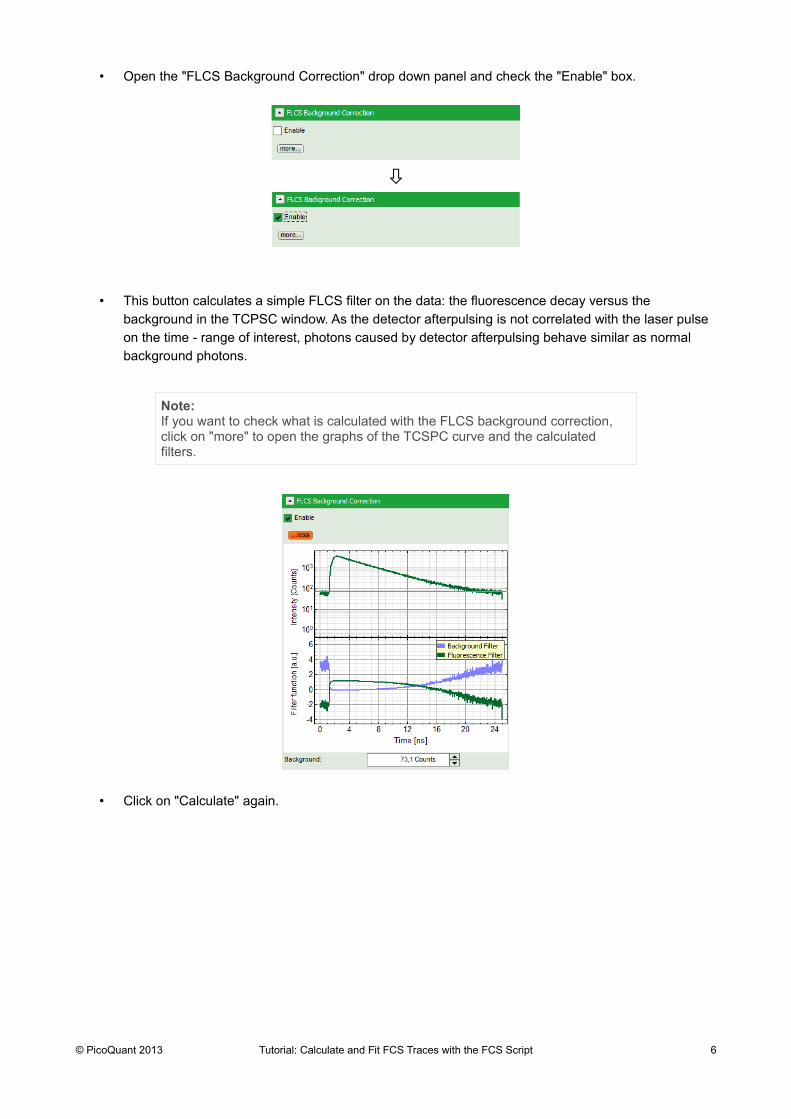
• Open the "FLCS Background Correction" drop down panel and check the "Enable" box.

• This button calculates a simple FLCS filter on the data: the fluorescence decay versus the background in the TCPSC window. As the detector afterpulsing is not correlated with the laser pulse on the time - range of interest, photons caused by detector afterpulsing behave similar as normal background photons.

• Click on "Calculate" again.


Note:If you want to check what is calculated with the FLCS background correction, click on "more" to open the graphs of the TCSPC curve and the calculated filters.

• It is not necessary to calculate first a FCS curve without the photon filter. You can also directly activate the FLCS background correction and calculate the FCS curve.

• Response: The FCS curve is re-calculated. As a result, the steep decrease at the beginning of the curve is now missing and an artifact free curve is obtained.

• If you do not want to fit the data: Save the calculated curve by clicking on "Save Result".

• Response: A result file is generated and linked to the raw data file.


Fitting FCS curves using the FCS Fitting script

• If you do want to fit the data: Transfer the curve to the FCS fitting script by clicking "Transfer to Fit".

• Response:

◦ The FCS curve is automatically stored. Therefore, it is not necessary to store the data before


Note:In order to provide correct results, the confocal volume VEff and the structural parameter κ have to be calculated first. Check the tutorial "Calibration of the confocal volume for FCS using the FCS Calibration Script" for a description about how to calibrate the confocal volume.

If no calibration values are stored, the effective volume VEff is set to 1 fl and the structural parameter κ is set to 5. While a structural parameter value of 5 is usually reasonable, the confocal volume depends on the wavelength and can differ significantly.

Check your system regularly for correct alignment using a reference dye as ATTO488.

In this tutorial, we use the default values to keep the description easy. If your system is already calibrated, the results (especially the concentration C and the diffusion constant D) will depend on your calibration.

transferring them to the FCS fitting script.

◦ The FCS Fitting window pops up.


Note:It is also possible to open a stored FCS curve directly with the FCS fitting script.

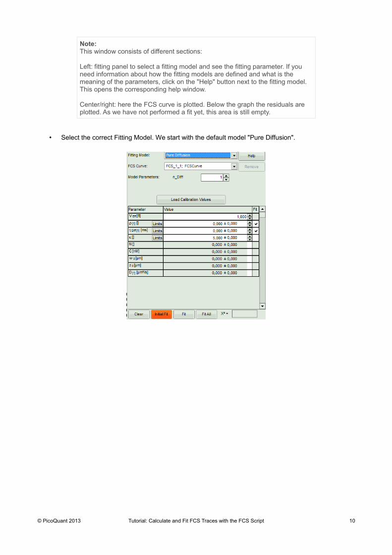
• Select the correct Fitting Model. We start with the default model "Pure Diffusion".


Note:This window consists of different sections:

Left: fitting panel to select a fitting model and see the fitting parameter. If you need information about how the fitting models are defined and what is the meaning of the parameters, click on the "Help" button next to the fitting model. This opens the corresponding help window.

Center/right: here the FCS curve is plotted. Below the graph the residuals are plotted. As we have not performed a fit yet, this area is still empty.

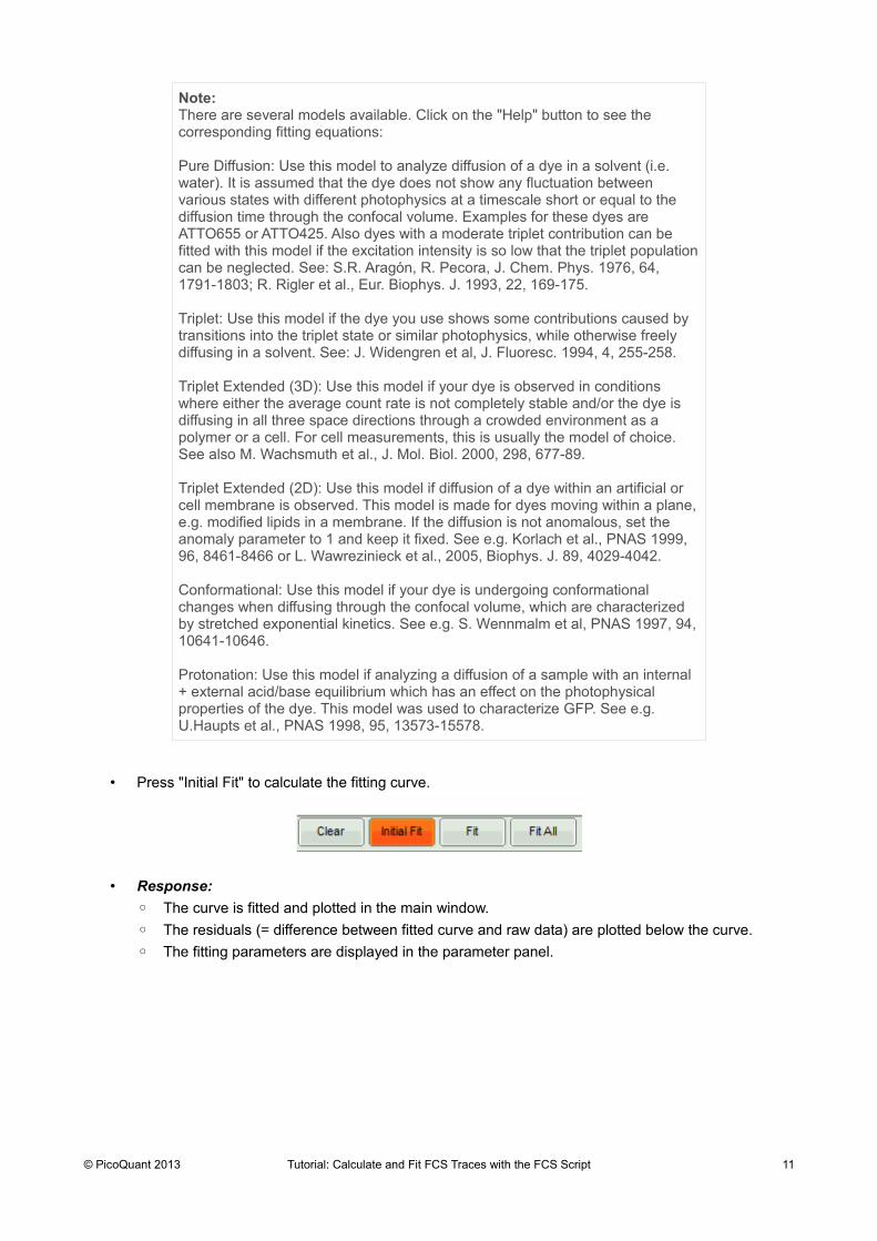
• Press "Initial Fit" to calculate the fitting curve.

• Response:

◦ The curve is fitted and plotted in the main window.

◦ The residuals (= difference between fitted curve and raw data) are plotted below the curve.

◦ The fitting parameters are displayed in the parameter panel.


Note:There are several models available. Click on the "Help" button to see the corresponding fitting equations:

Pure Diffusion: Use this model to analyze diffusion of a dye in a solvent (i.e. water). It is assumed that the dye does not show any fluctuation between various states with different photophysics at a timescale short or equal to the diffusion time through the confocal volume. Examples for these dyes are ATTO655 or ATTO425. Also dyes with a moderate triplet contribution can be fitted with this model if the excitation intensity is so low that the triplet populationcan be neglected. See: S.R. Aragón, R. Pecora, J. Chem. Phys. 1976, 64, 1791-1803; R. Rigler et al., Eur. Biophys. J. 1993, 22, 169-175.

Triplet: Use this model if the dye you use shows some contributions caused by transitions into the triplet state or similar photophysics, while otherwise freely diffusing in a solvent. See: J. Widengren et al, J. Fluoresc. 1994, 4, 255-258.

Triplet Extended (3D): Use this model if your dye is observed in conditions where either the average count rate is not completely stable and/or the dye is diffusing in all three space directions through a crowded environment as a polymer or a cell. For cell measurements, this is usually the model of choice. See also M. Wachsmuth et al., J. Mol. Biol. 2000, 298, 677-89.

Triplet Extended (2D): Use this model if diffusion of a dye within an artificial or cell membrane is observed. This model is made for dyes moving within a plane,e.g. modified lipids in a membrane. If the diffusion is not anomalous, set the anomaly parameter to 1 and keep it fixed. See e.g. Korlach et al., PNAS 1999, 96, 8461-8466 or L. Wawrezinieck et al., 2005, Biophys. J. 89, 4029-4042.

Conformational: Use this model if your dye is undergoing conformational changes when diffusing through the confocal volume, which are characterized by stretched exponential kinetics. See e.g. S. Wennmalm et al, PNAS 1997, 94,10641-10646.

Protonation: Use this model if analyzing a diffusion of a sample with an internal + external acid/base equilibrium which has an effect on the photophysical properties of the dye. This model was used to characterize GFP. See e.g. U.Haupts et al., PNAS 1998, 95, 13573-15578.

• Select the "Triplet" model.

• Response: The parameters in the parameter panel are adapted.

• Press "Initial Fit".


Note:It can be clearly seen that at short correlation time ranges, the curve does not fitthe data well. This is an indicator that the sample undergoes some photophysical fluctuations in the µs – time range, usually triplet fluctuations. Therefore, we have to change the fitting model.

• Response:

◦ The curve is fitted and plotted in the main window.

◦ The residuals (= difference between fitted curve and raw data) are plotted below the curve.

◦ The fitting parameters are displayed in the parameter panel.

• Save the fit by clicking "Save Results".


Note:This time, the curve fits the data significantly better.

A diffusion time of a few tens of µs is typical for a dye in water, as well as triplet time in the range of a few microseconds.

The fitted diffusion coefficient D is significantly higher than the real value of 400µm²/s. This is due to the incorrect calibration. If the diffusion coefficient is known, the size of the confocal volume can be decreased and the curve refitted,until the fitted diffusion coefficient is realistic.

Please look at the corresponding tutorial to learn how to calibrate the confocal volume.

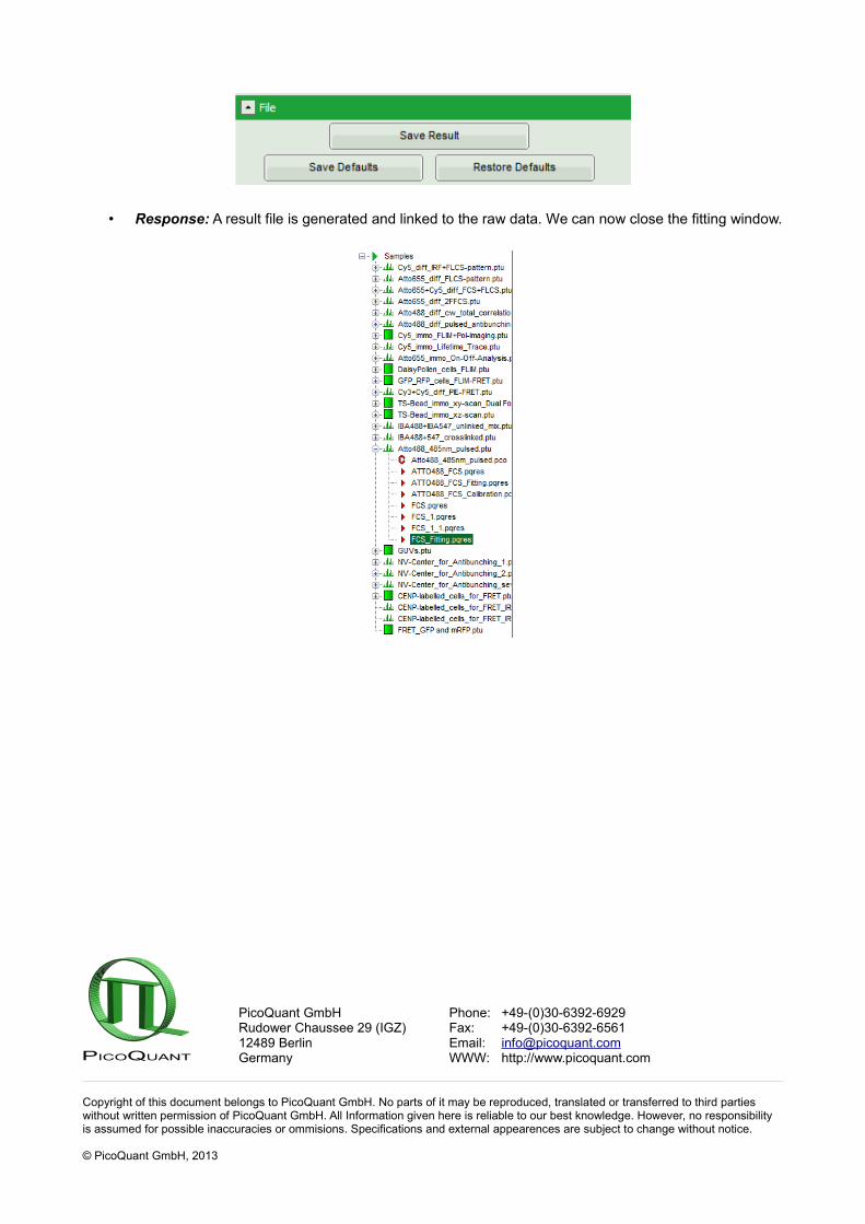
• Response: A result file is generated and linked to the raw data. We can now close the fitting window.

PicoQuant GmbH Phone: +49-(0)30-6392-6929Rudower Chaussee 29 (IGZ) Fax: +49-(0)30-6392-656112489 Berlin Email: [email protected] WWW: http://www.picoquant.com

Copyright of this document belongs to PicoQuant GmbH. No parts of it may be reproduced, translated or transferred to third parties without written permission of PicoQuant GmbH. All Information given here is reliable to our best knowledge. However, no responsibility is assumed for possible inaccuracies or ommisions. Specifications and external appearences are subject to change without notice.

© PicoQuant GmbH, 2013

fff

mailto:[email protected]

http://www.picoquant.com/

Documents

Calculate and Fit FCS Traces with the FCS Script - … · Tutorial Calculate and Fit FCS Traces with the FCS Script Summary This tutorial shows step-by-step, how an autocorrelation