(c) 2007 IUPUI SPEA K300 (4392)

Outline

Random VariablesExpected ValuesData Generation Process (DGP)Uniform Probability DistributionBinomial Probability Distribution

(c) 2007 IUPUI SPEA K300 (4392)

Random Variables

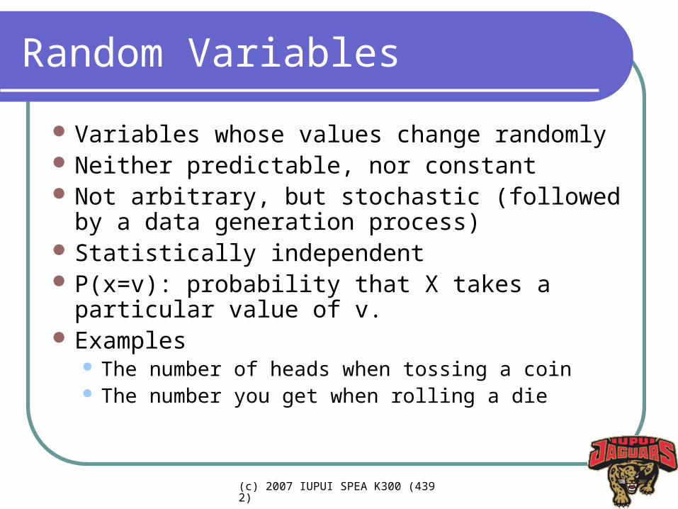
Variables whose values change randomly Neither predictable, nor constant Not arbitrary, but stochastic (followed by a

data generation process) Statistically independent P(x=v): probability that X takes a particular

value of v. Examples

The number of heads when tossing a coin The number you get when rolling a die

(c) 2007 IUPUI SPEA K300 (4392)

Discrete versus Continuous

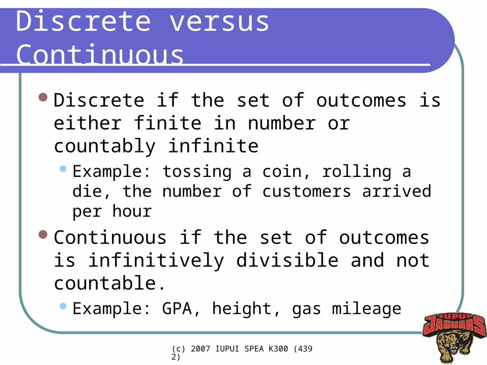
Discrete if the set of outcomes is either finite in number or countably infiniteExample: tossing a coin, rolling a die, the

number of customers arrived per hourContinuous if the set of outcomes is

infinitively divisible and not countable. Example: GPA, height, gas mileage

(c) 2007 IUPUI SPEA K300 (4392)

Level of Measurement

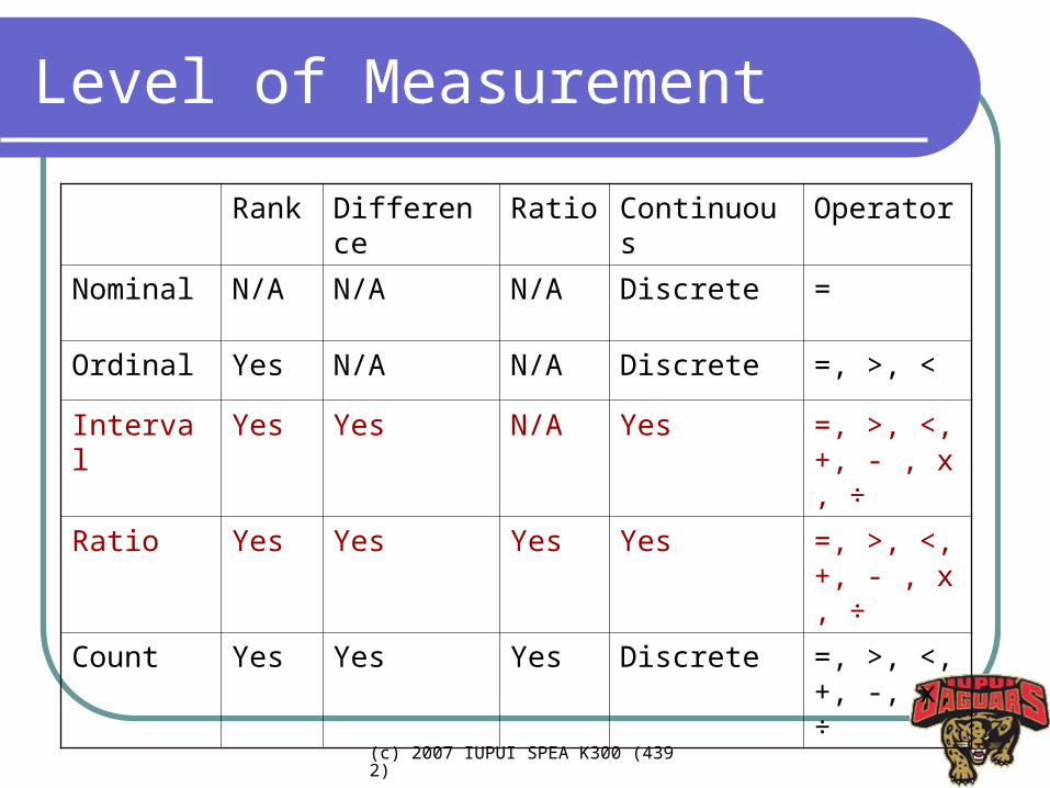
Rank Difference Ratio Continuous Operator

Nominal N/A N/A N/A Discrete =

Ordinal Yes N/A N/A Discrete =, >, <

Interval Yes Yes N/A Yes =, >, <, +, - , x , ÷

Ratio Yes Yes Yes Yes =, >, <, +, - , x , ÷

Count Yes Yes Yes Discrete =, >, <, +, -, x, ÷

(c) 2007 IUPUI SPEA K300 (4392)

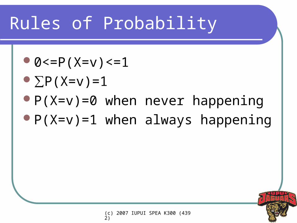
Rules of Probability

0<=P(X=v)<=1∑P(X=v)=1P(X=v)=0 when never happeningP(X=v)=1 when always happening

(c) 2007 IUPUI SPEA K300 (4392)

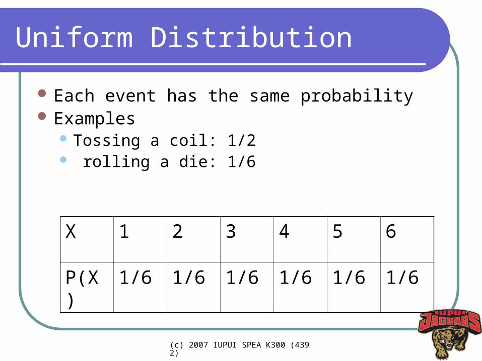
Uniform Distribution

Each event has the same probability Examples

Tossing a coil: 1/2 rolling a die: 1/6

X 1 2 3 4 5 6

P(X) 1/6 1/6 1/6 1/6 1/6 1/6

(c) 2007 IUPUI SPEA K300 (4392)

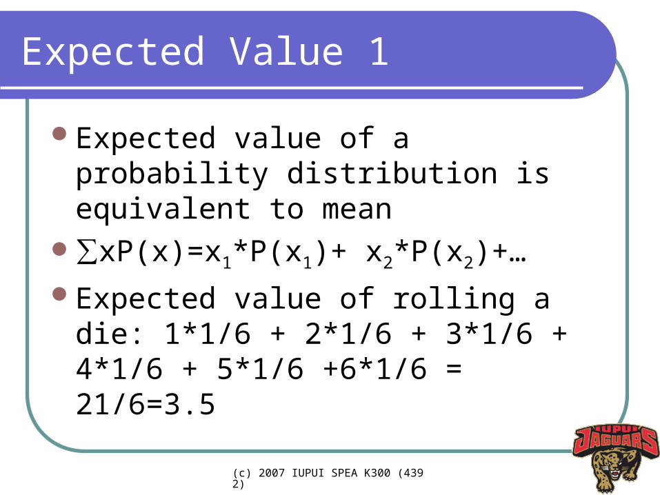
Expected Value 1

Expected value of a probability distribution is equivalent to mean

∑xP(x)=x1*P(x1)+ x2*P(x2)+…

Expected value of rolling a die: 1*1/6 + 2*1/6 + 3*1/6 + 4*1/6 + 5*1/6 +6*1/6 = 21/6=3.5

(c) 2007 IUPUI SPEA K300 (4392)

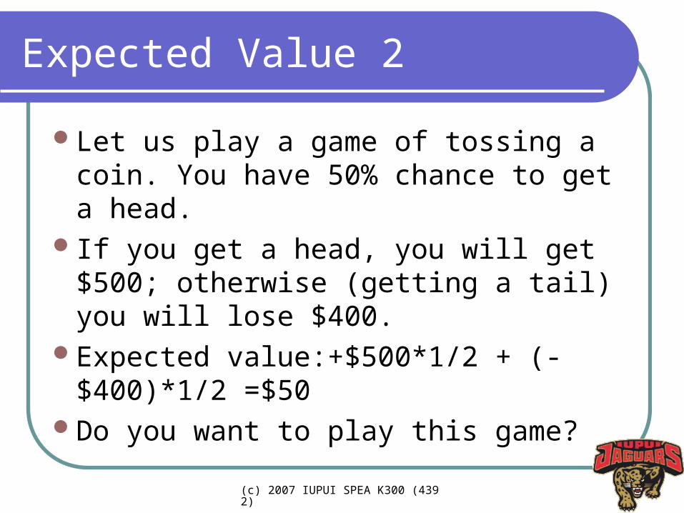
Expected Value 2

Let us play a game of tossing a coin. You have 50% chance to get a head.

If you get a head, you will get $500; otherwise (getting a tail) you will lose $400.

Expected value:+$500*1/2 + (-$400)*1/2 =$50

Do you want to play this game?

(c) 2007 IUPUI SPEA K300 (4392)

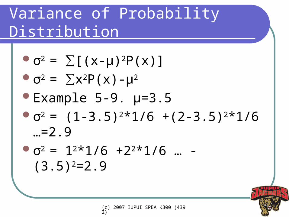
Variance of Probability Distribution

σ2 = ∑[(x-µ)2P(x)] σ2 = ∑x2P(x)-µ2 Example 5-9. µ=3.5σ2 = (1-3.5)2*1/6 +(2-3.5)2*1/6 …=2.9σ2 = 12*1/6 +22*1/6 … -(3.5)2=2.9

(c) 2007 IUPUI SPEA K300 (4392)

Data Generation Process (DGP)

How are data (random variables) generated?

“Tossing a coin” is a DGP that has only two outcomes (head/tail) with equal P

“Rolling a die” is a DGP that has six outcomes with equal P (1/6)

How about GPA of SPEA students?How do we formulate these DGPs

(c) 2007 IUPUI SPEA K300 (4392)

Binomial Experiment

Each trial: Bernoulli process (or trial)There must be a fixed number of trials, nEach trial can have only two outcomes, x

(yes/no, true/false, success/failure)The outcome of each trial must be

(statistically) independent of each otherThe probability of a success, p, must

remain the same for each trial

(c) 2007 IUPUI SPEA K300 (4392)

Binomial Distribution 1

Consists of N times of the Bernoulli trial with two outcomes

Probabilities of these outcomes, which are not necessarily equal

Examples: What is the probability that you will get 10 heads

when tossing a coin 20 times? Given .01 of getting a certain disease, what is the

probability that 5 out of 10 randomly selected subjects get the disease?

(c) 2007 IUPUI SPEA K300 (4392)

Binomial Distribution 2

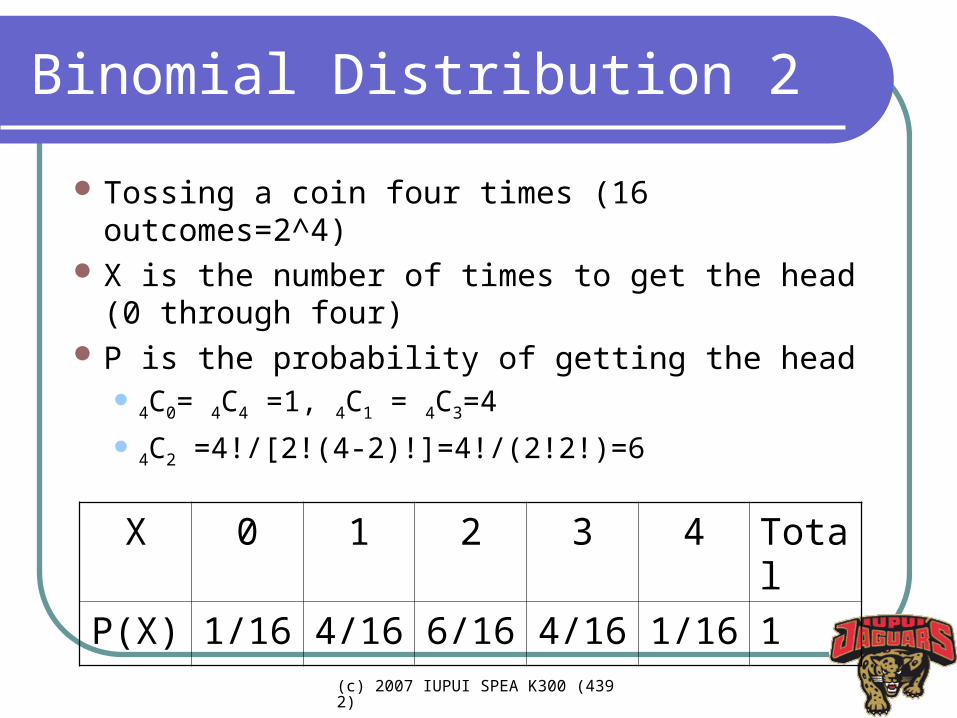
Tossing a coin four times (16 outcomes=2^4) X is the number of times to get the head (0

through four) P is the probability of getting the head

4C0= 4C4 =1, 4C1 = 4C3=4

4C2 =4!/[2!(4-2)!]=4!/(2!2!)=6

X 0 1 2 3 4 Total

P(X) 1/16 4/16 6/16 4/16 1/16 1

(c) 2007 IUPUI SPEA K300 (4392)

Binomial Distribution 3

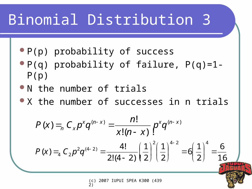
P(p) probability of successP(q) probability of failure, P(q)=1-P(p)N the number of trialsX the number of successes in n trials

)()(

)!(!

!)( xnxxnx

xn qpxnx

nqpCxP

16

6

2

16

2

1

2

1

)!24(!2

!4)(

4242)24(2

24

qpCxP

(c) 2007 IUPUI SPEA K300 (4392)

Binomial Distribution 4

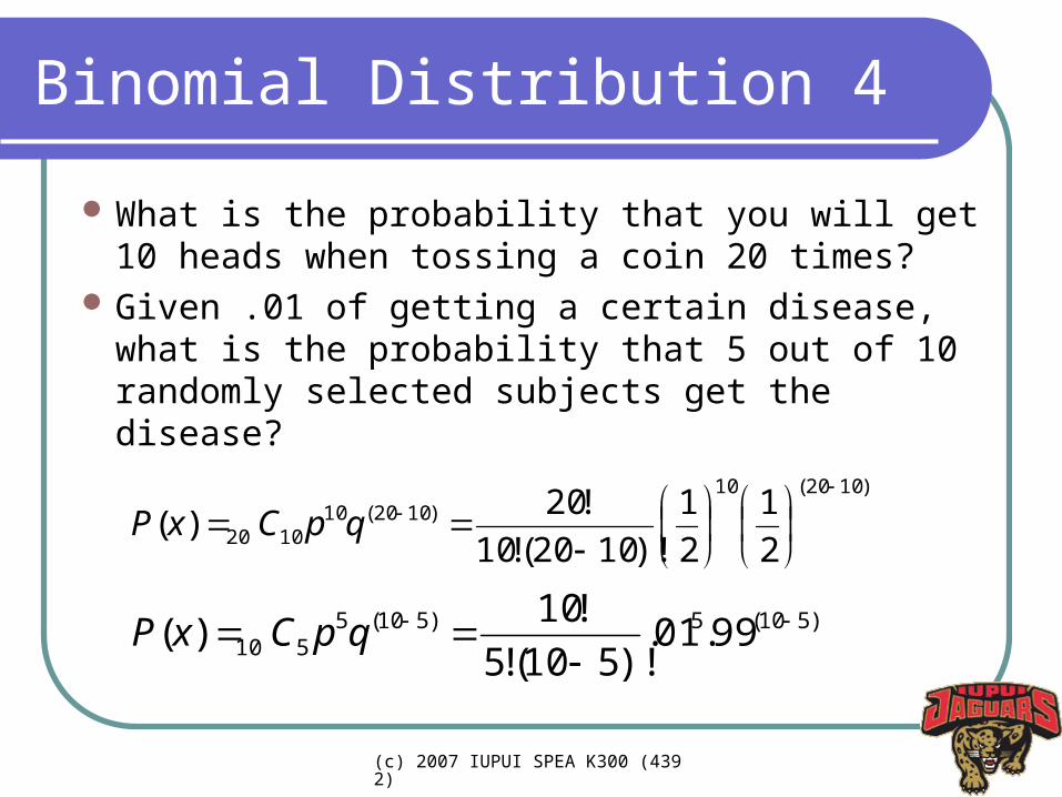
What is the probability that you will get 10 heads when tossing a coin 20 times?

Given .01 of getting a certain disease, what is the probability that 5 out of 10 randomly selected subjects get the disease?

)510(5)510(5510 99.01.

)!510(!5

!10)(

qpCxP

)1020(10)1020(10

1020 2

1

2

1

)!1020(!10

!20)(

qpCxP

(c) 2007 IUPUI SPEA K300 (4392)

Binomial Distribution 5

Sick and tired of the formula? Good news. Someone computed the

probability of binomial distribution for you. See example 5-18, p 265.

What you have to know is N, X, and PGo to page 626What is the probability that 5 out of 10

get the disease? P=.01

(c) 2007 IUPUI SPEA K300 (4392)

Binomial Distribution 6

Expected value: µ=npVariance: npqStandard deviation: sqrt(npq)Example 5.21, p. 267.

µ=np=4 X ½= 2σ2 =npq=4X½ X½ =1σ=sqrt(1)=1

(c) 2007 IUPUI SPEA K300 (4392)

Illustration 0

Tossing a coinTwo outcomes: head and tailP(head)=1/2http://www.uwsp.edu/psych/stat/9/

hyptestd.htm

(c) 2007 IUPUI SPEA K300 (4392)

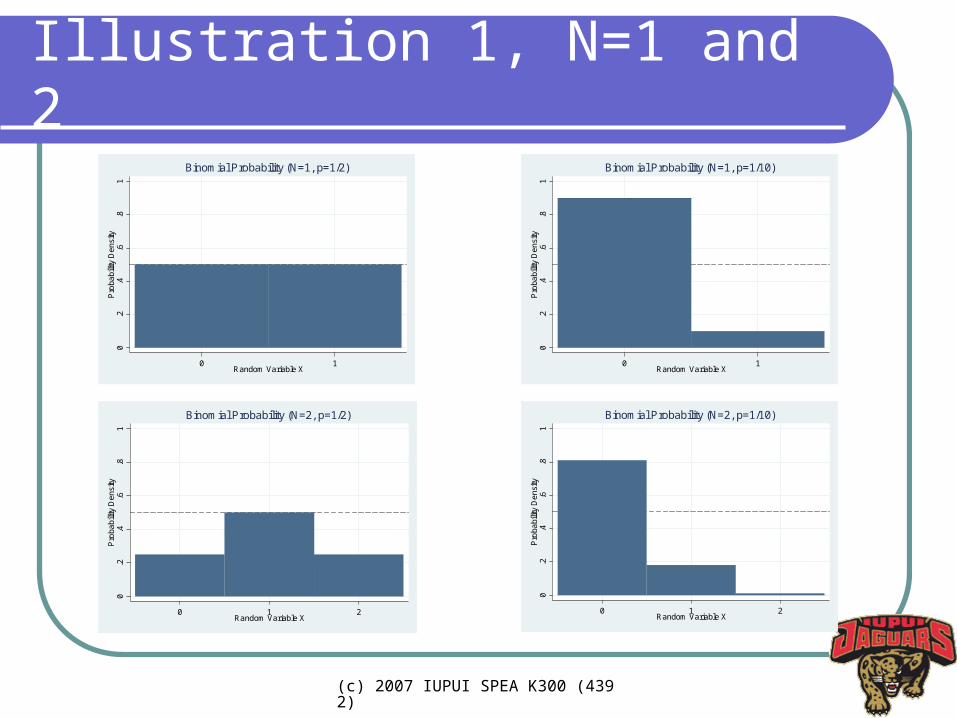
Illustration 1, N=1 and 20

.2.4

.6.8

1P

roba

bilit

y D

ens

ity

0 1Random Variable X

Binomial Probability (N=1, p=1/2)

0.2

.4.6

.81

Pro

babi

lity

De

nsity

0 1 2Random Variable X

Binomial Probability (N=2, p=1/2)

0.2

.4.6

.81

Pro

babi

lity

De

nsity

0 1Random Variable X

Binomial Probability (N=1, p=1/10)

0.2

.4.6

.81

Pro

babi

lity

De

nsity

0 1 2Random Variable X

Binomial Probability (N=2, p=1/10)

(c) 2007 IUPUI SPEA K300 (4392)

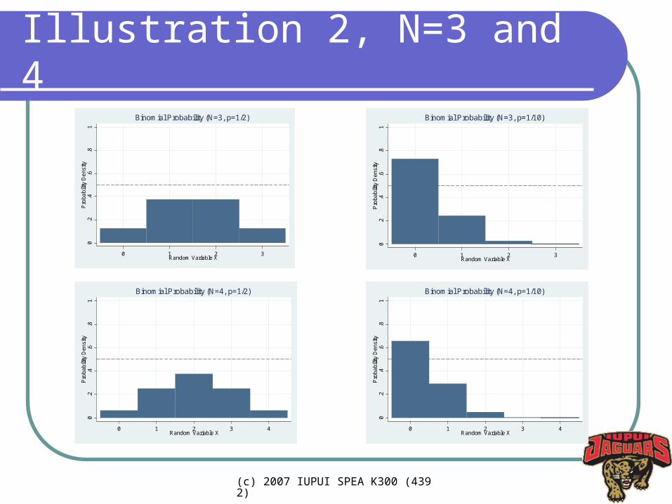
Illustration 2, N=3 and 40

.2.4

.6.8

1P

roba

bilit

y D

ens

ity

0 1 2 3Random Variable X

Binomial Probability (N=3, p=1/2)

0.2

.4.6

.81

Pro

babi

lity

De

nsity

0 1 2 3 4Random Variable X

Binomial Probability (N=4, p=1/2)

0.2

.4.6

.81

Pro

babi

lity

De

nsity

0 1 2 3Random Variable X

Binomial Probability (N=3, p=1/10)

0.2

.4.6

.81

Pro

babi

lity

De

nsity

0 1 2 3 4Random Variable X

Binomial Probability (N=4, p=1/10)

(c) 2007 IUPUI SPEA K300 (4392)

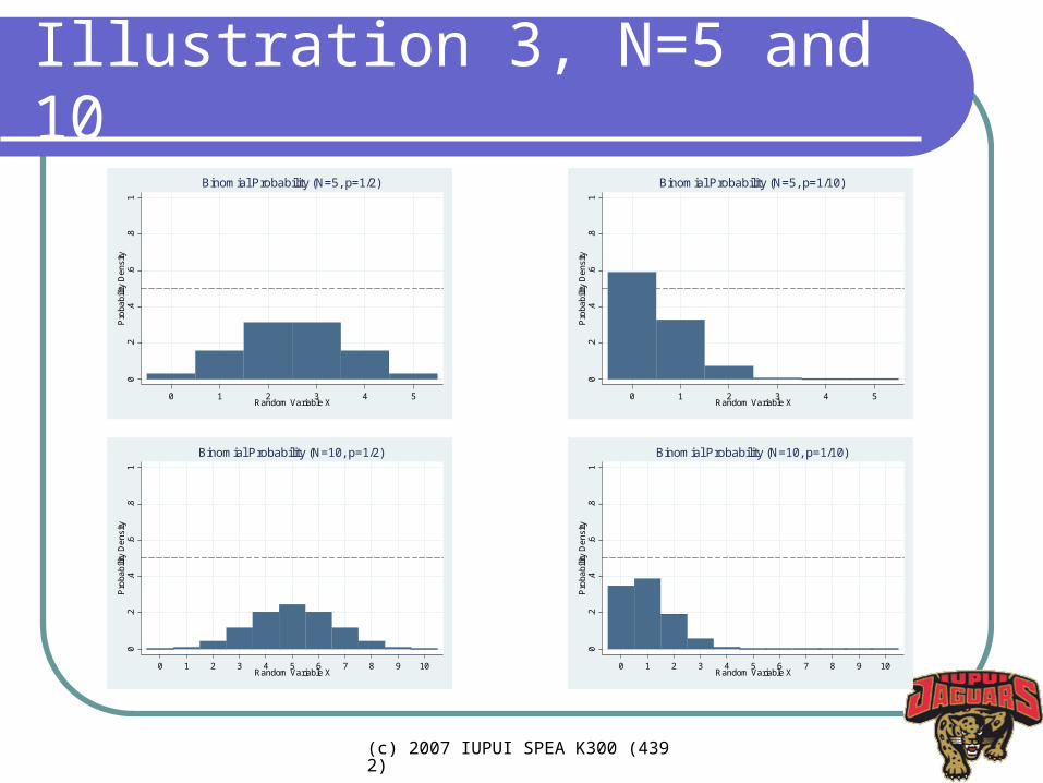
Illustration 3, N=5 and 100

.2.4

.6.8

1P

roba

bilit

y D

ens

ity

0 1 2 3 4 5 6 7 8 9 10Random Variable X

Binomial Probability (N=10, p=1/2)

0.2

.4.6

.81

Pro

babi

lity

De

nsity

0 1 2 3 4 5Random Variable X

Binomial Probability (N=5, p=1/2)

0.2

.4.6

.81

Pro

babi

lity

De

nsity

0 1 2 3 4 5Random Variable X

Binomial Probability (N=5, p=1/10)

0.2

.4.6

.81

Pro

babi

lity

De

nsity

0 1 2 3 4 5 6 7 8 9 10Random Variable X

Binomial Probability (N=10, p=1/10)

(c) 2007 IUPUI SPEA K300 (4392)

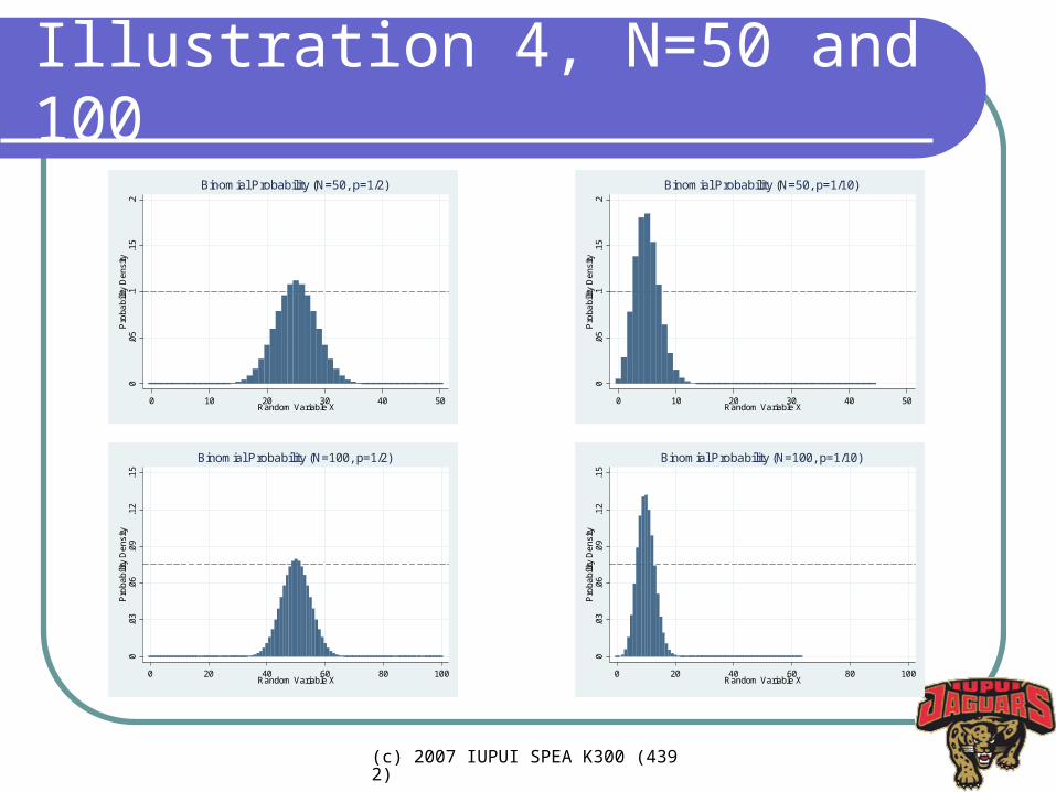
Illustration 4, N=50 and 100

0.0

3.0

6.0

9.1

2.1

5P

roba

bilit

y D

ens

ity

0 20 40 60 80 100Random Variable X

Binomial Probability (N=100, p=1/10)

0.0

5.1

.15

.2P

roba

bilit

y D

ens

ity

0 10 20 30 40 50Random Variable X

Binomial Probability (N=50, p=1/10)

0.0

3.0

6.0

9.1

2.1

5P

roba

bilit

y D

ens

ity

0 20 40 60 80 100Random Variable X

Binomial Probability (N=100, p=1/2)

0.0

5.1

.15

.2P

roba

bilit

y D

ens

ity

0 10 20 30 40 50Random Variable X

Binomial Probability (N=50, p=1/2)

(c) 2007 IUPUI SPEA K300 (4392)

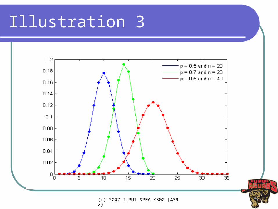
Illustration 3