Embed Size (px)
Citation preview

(c) 2007 IUPUI SPEA K300 (4392)
Outline
Least Squares MethodsEstimation: Least SquaresInterpretation of estimatorsProperties of OLS estimatorsVariance of Y, b, and aHypothesis Test of b and aANOVA tableGoodness-of-Fit and R2

(c) 2007 IUPUI SPEA K300 (4392)
Linear regression model
1
.5
12
45
3y
-1 0 1 2 3 4 5x
Y = 2 +.5X

(c) 2007 IUPUI SPEA K300 (4392)
Terminology
Dependent variable (DV) = response variable = left-hand side (LHS) variable
Independent variables (IV) = explanatory variables = right-hand side (RHS) variables = regressor (excluding a or b0)
a (b0) is an estimator of parameter α, β0
b (b1) is an estimator of parameter β, β1
a and b are the intercept and slope

(c) 2007 IUPUI SPEA K300 (4392)
Least Squares Method
How to draw such a line based on data points observed?
Suppose a imaginary line of y= a + bx Imagine a vertical distance (or error) between
the line and a data point. E=Y-E(Y) This error (or gap) is the deviation of the data
point from the imaginary line, regression line What is the best values of a and b? A and b that minimizes the sum of such errors
(deviations of individual data points from the line)

(c) 2007 IUPUI SPEA K300 (4392)
Least Squares Method
E(Y)=a + bX
e1
x1
x2
x3
e2
e3
01
23
4y
0 1 2 3 4 5x
Least Squares Method

(c) 2007 IUPUI SPEA K300 (4392)
Least Squares Method
Deviation does not have good properties for computation
Why do we use squares of deviation? (e.g., variance)
Let us get a and b that can minimize the sum of squared deviations rather than the sum of deviations.
This method is called least squares

(c) 2007 IUPUI SPEA K300 (4392)
Least Squares Method
Least squares method minimizes the sum of squares of errors (deviations of individual data points form the regression line)
Such a and b are called least squares estimators (estimators of parameters α and β).
The process of getting parameter estimators (e.g., a and b) is called estimation
“Regress Y on X” Lest squares method is the estimation method
of ordinary least squares (OLS)
(c) 2007 IUPUI SPEA K300 (4392)
Ordinary Least Squares
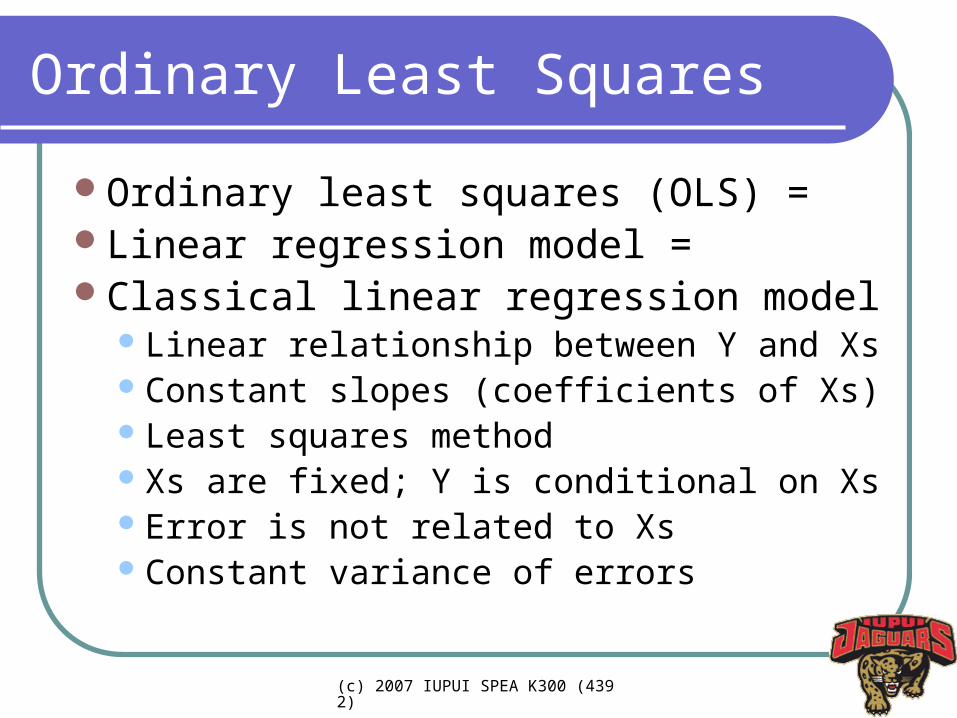
Ordinary least squares (OLS) = Linear regression model =Classical linear regression model
Linear relationship between Y and XsConstant slopes (coefficients of Xs)Least squares methodXs are fixed; Y is conditional on XsError is not related to XsConstant variance of errors

(c) 2007 IUPUI SPEA K300 (4392)
Least Squares Method 1
XY
bXaYYE ˆ)(
bXaYbXaYYY )(ˆ222 )()ˆ( bXaYYY
222 )()ˆ( bXaYYY
abXbXYaYXbaYbXaY 222)( 22222
22 )( bXaYMinMin
How to get a and b that can minimize the sum of squares of errors?

(c) 2007 IUPUI SPEA K300 (4392)
Least Squares Method 2
• Linear algebraic solution
• Compute a and b so that partial derivatives with respect to a and b are equal to zero
0222
)( 22
XbYnaa
bXaY
a
0 XbYna
XbYn
Xb
n
Ya

(c) 2007 IUPUI SPEA K300 (4392)
Least Squares Method 3
Take a partial derivative with respect to b and plug in a you got, a=Ybar –b*Xbar
0222
)( 222
XaXYXbb
bXaY
b
02 XaXYXb 02 XXbYXYXb
02
X
n
Xb
n
YXYXb
0
2
2 n
Xb
n
YXXYXb
n
YXXY
n
XXnb
22

(c) 2007 IUPUI SPEA K300 (4392)
Least Squares Method 4
Least squares method is an algebraic solution that minimizes the sum of squares of errors (variance component of error)
x
xy
SS
SP
XX
YYXX
XXn
YXXYnb
222 )(
))((
XbYn
Xb
n
Ya
22
2
XXn
XYXXYa Not recommended

(c) 2007 IUPUI SPEA K300 (4392)
OLS: Example 10-5 (1)
No x y x-xbar y-ybar (x-xb)(y-yb) (x-xbar)^2
1 43 128 -14.5 -8.5 123.25 210.25
2 48 120 -9.5 -16.5 156.75 90.25
3 56 135 -1.5 -1.5 2.25 2.25
4 61 143 3.5 6.5 22.75 12.25
5 67 141 9.5 4.5 42.75 90.25
6 70 152 12.5 15.5 193.75 156.25
Mean 57.5 136.5
Sum 345 819 541.5 561.5
0481.815.579644.5.136 XbYa
9644.5.561
5.541
)(
))((2
x
xy
SS
SP
XX
YYXXb

(c) 2007 IUPUI SPEA K300 (4392)
OLS: Example 10-5 (2), NO!
048.81345203996
4763434520399819222
2
XXn
XYXXYa
964.345203996
819345476346222
XXn
YXXYnb
No x y xy x^2
1 43 128 5504 1849
2 48 120 5760 2304
3 56 135 7560 3136
4 61 143 8723 3721
5 67 141 9447 4489
6 70 152 10640 4900
Mean 57.5 136.5
Sum 345 819 47634 20399

(c) 2007 IUPUI SPEA K300 (4392)
OLS: Example 10-5 (3)1
201
301
401
50
40 50 60 70x
Fitted values y
Y hat = 81.048 + .964X

(c) 2007 IUPUI SPEA K300 (4392)
What Are a and b ?
a is an estimator of its parameter αa is the intercept, a point of y where the
regression line meets the y axisb is an estimator of its parameter βb is the slope of the regression lineb is constant regardless of values of Xsb is more important than a since that is
what researchers want to know.

(c) 2007 IUPUI SPEA K300 (4392)
How to interpret b?
For unit increase in x, the expected change in y is b, holding other things (variables) constant.
For unit increase in x, we expect that y increases by b, holding other things (variables) constant.
For unit increase in x, we expect that y increases by .964, holding other variables constant.

(c) 2007 IUPUI SPEA K300 (4392)
Properties of OLS estimators
The outcome of least squares method is OLS parameter estimators a and b.
OLS estimators are linear OLS estimators are unbiased (precise) OLS estimators are efficient (small variance) Gauss-Markov Theorem: Among linear
unbiased estimators, least square estimator (OLS estimator) has minimum variance. BLUE (best linear unbiased estimator)

(c) 2007 IUPUI SPEA K300 (4392)
Hypothesis Test of a an b
How reliable are a and b we compute? T-test (Wald test in general) can answer The standardized effect size (effect size /
standard error) Effect size is a-0 and b-0 assuming 0 is the
hypothesized value; H0: α=0, H0: β=0
Degrees of freedom is N-K, where K is the number of regressors +1
How to compute standard error (deviation)?

(c) 2007 IUPUI SPEA K300 (4392)
Variance of b (1)
b is a random variable that changes across samples.
b is a weighted sum of linear combinations of random variable Y
iiYwXX
YXX
XX
YXnXY
XX
YYXX222 )(
)(
)()(
))((
nnii YwYwYwYw ...2211
2)(
)(
XX
XXw
i
ii
YXnXYYXnYnXXnYXYYXnYXXYXY
YXYXYXXYYXYXYXXYYYXX
)())((

(c) 2007 IUPUI SPEA K300 (4392)
Variance of b (2)
Variance of Y (error) is σ2
Var(kY) = k2Var(Y) = k2σ2
222222
222
1
22
221
21
...
)(...)()()()ˆ(
in
nnii
wwww
YVarwYVarwYVarwYwVarVar
2
22
22
22
2222
)()(
)()(
)(
XXXX
XXXX
XXw
ii
ii
ii
iiYwXX
YYXXb 2)(
))((
2)(
)(
XX
XXw
i
ii

(c) 2007 IUPUI SPEA K300 (4392)
Variance of a
a=Ybar + b*Xbar Var(b)=σ2/SSx , SSx = ∑(X-Xbar)2
Var(∑Y)=Var(Y1)+Var(Y2)+…+Var(Yn)=nσ2
2
22
2
222
2
2
22
22
)(
1
)(
1
)()(
1)(
),(2)()()()ˆ(
XX
X
nXXXn
n
XXXYVar
nbVarX
n
YVar
XbYCovXbVarYVarXbYVarVar
ii
i
Now, how do we compute the variance of Y, σ2?

(c) 2007 IUPUI SPEA K300 (4392)
Variance of Y or error
Variance of Y is based on residuals (errors), Y-Yhat
“Hat” means an estimator of the parameter Y hat is predicted (by a + bX) value of Y; plug in
x given a and b to get Y hat Since a regression model includes K
parameters (a and b in simple regression), the degrees of freedom is N-K
Numerator is SSE in the ANOVA table
MSEKN
SSE
KN
YYs iie
222 )ˆ(

(c) 2007 IUPUI SPEA K300 (4392)
Illustration (1)
No x y x-xbar y-ybar (x-xb)(y-yb) (x-xbar)^2 yhat (y-yhat)^2
1 43 128 -14.5 -8.5 123.25 210.25 122.52 30.07
2 48 120 -9.5 -16.5 156.75 90.25 127.34 53.85
3 56 135 -1.5 -1.5 2.25 2.25 135.05 0.00
4 61 143 3.5 6.5 22.75 12.25 139.88 9.76
5 67 141 9.5 4.5 42.75 90.25 145.66 21.73
6 70 152 12.5 15.5 193.75 156.25 148.55 11.87
Mean 57.5 136.5
Sum 345 819 541.5 561.5 127.2876
8219.3126
2876.127)ˆ( 22
KN
YYs iie
22
2
2381.0567.5.561
8219.31
)(
ˆ)ˆ()(
XX
VarbVari
SSE=127.2876, MSE=31.8219
22
2
22 8809.13
5.561
5.57
6
18219.31
)(
1ˆ)(
XX
X
naVar
i

(c) 2007 IUPUI SPEA K300 (4392)
Illustration (2): Test b
How to test whether beta is zero (no effect)? Like y, α and β follow a normal distribution; a
and b follows the t distribution b=.9644, SE(b)=.2381,df=N-K=6-2=4 Hypothesis Testing
1. H0:β=0 (no effect), Ha:β≠0 (two-tailed) 2. Significance level=.05, CV=2.776, df=6-2=4 3. TS=(.9644-0)/.2381=4.0510~t(N-K) 4. TS (4.051)>CV (2.776), Reject H0 5. Beta (not b) is not zero. There is a significant
impact of X on Y2381.776.29644.
)(
1ˆ2211
XXst
ie
(c) 2007 IUPUI SPEA K300 (4392)
Illustration (3): Test a
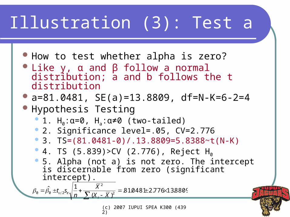
How to test whether alpha is zero? Like y, α and β follow a normal distribution; a
and b follows the t distribution a=81.0481, SE(a)=13.8809, df=N-K=6-2=4 Hypothesis Testing
1. H0:α=0, Ha:α≠0 (two-tailed) 2. Significance level=.05, CV=2.776 3. TS=(81.0481-0)/.13.8809=5.8388~t(N-K) 4. TS (5.839)>CV (2.776), Reject H0 5. Alpha (not a) is not zero. The intercept is
discernable from zero (significant intercept).8809.13776.20481.81.
)(
1ˆ2
2
200
XX
X
nst
ie
(c) 2007 IUPUI SPEA K300 (4392)
Questions
How do we test H0: β0(α)=β1=β2 …=0?
Remember that t-test compares only two group means, while ANOVA compares more than two group means simultaneously.
The same thing in linear regression. Construct the ANOVA table by partitioning
variance of Y; F test examines the above H0
The ANOVA table provides key information of a regression model

(c) 2007 IUPUI SPEA K300 (4392)
Partitioning Variance of Y (1)
Yi
Ybar=136.5
Yhat=81+.96X
120
130
140
150
40 50 60 70x
Fitted values y
Y hat = 81.048 + .964X, Ybar=136.5
(c) 2007 IUPUI SPEA K300 (4392)
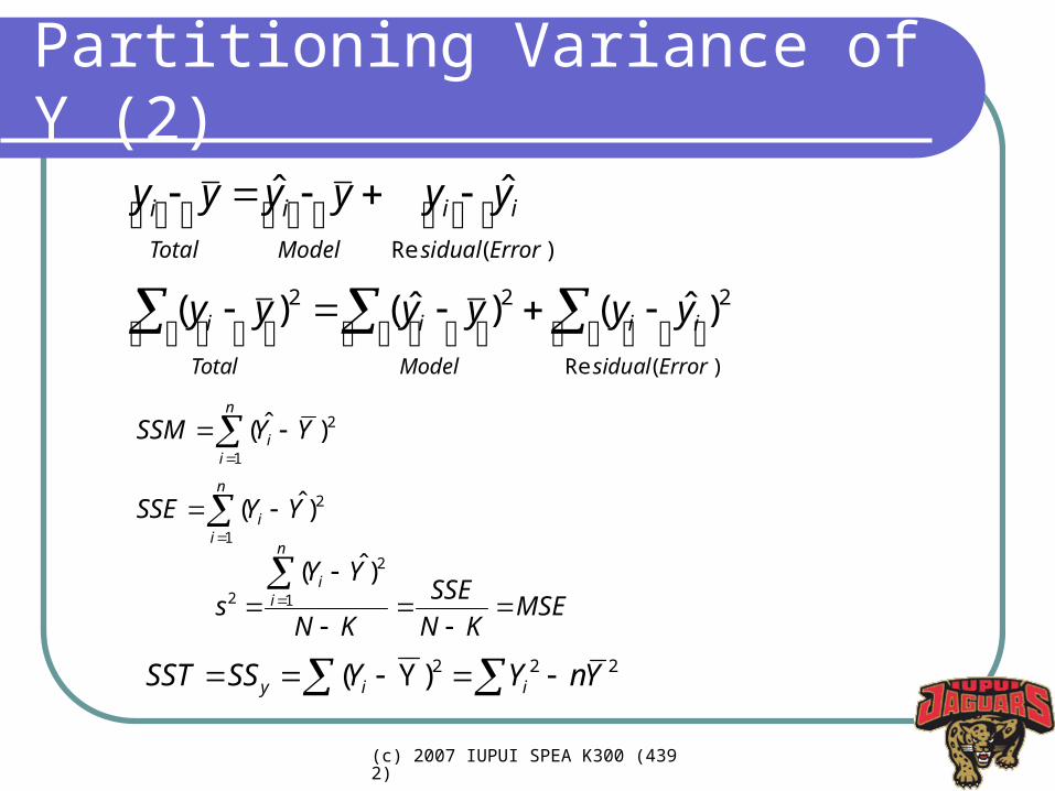
Partitioning Variance of Y (2)
)(Re
ˆˆErrorsidual
ii
Model
i
Total
i yyyyyy
)(Re
222 )ˆ()ˆ()(
Errorsidual
ii
Model
i
Total
i yyyyyy
222)Y( YnYYSSSST iiy
n
ii YYSSE
1
2)ˆ(
MSEKN
SSE
KN
YYs
n
ii
1
2
2
)ˆ(
n
ii YYSSM
1
2)ˆ(

(c) 2007 IUPUI SPEA K300 (4392)
Partitioning Variance of Y (3)
81+.96X
No x y yhat (y-ybar)^2 (yhat-ybar)^2 (y-yhat)^2
1 43 128 122.52 72.25 195.54 30.07
2 48 120 127.34 272.25 83.94 53.85
3 56 135 135.05 2.25 2.09 0.00
4 61 143 139.88 42.25 11.39 9.76
5 67 141 145.66 20.25 83.94 21.73
6 70 152 148.55 240.25 145.32 11.87
Mean 57.5 136.5 SST SSM SSE
Sum 345 819 649.5000 522.2124 127.2876
•122.52=81+.96×43, 148.6=.81+.96×70
•SST=SSM+SSE, 649.5=522.2+127.3

(c) 2007 IUPUI SPEA K300 (4392)
ANOVA Table
H0: all parameters are zero, β0 = β1 = 0 Ha: at least one parameter is not zero CV is 12.22 (1,4), TS>CV, reject H0
Sources Sum of Squares DF Mean Squares F
Model SSM K-1 MSM=SSM/(K-1) MSM/MSE
Residual SSE N-K MSE=SSE/(N-K)
Total SST N-1
Sources Sum of Squares DF Mean Squares F
Model 522.2124 1 522.2124 16.41047
Residual 127.2876 4 31.8219
Total 649.5000 5

(c) 2007 IUPUI SPEA K300 (4392)
R2 and Goodness-of-fit
Goodness-of-fit measures evaluates how well a regression model fits the data
The smaller SSE, the better fit the model F test examines if all parameters are zero.
(large F and small p-value indicate good fit) R2 (Coefficient of Determination) is SSM/SST
that measures how much a model explains the overall variance of Y.
R2=SSM/SST=522.2/649.5=.80 Large R square means the model fits the data

(c) 2007 IUPUI SPEA K300 (4392)
Myth and Misunderstanding in R2
R square is Karl Pearson correlation coefficient squared. r2=.89672=.80
If a regression model includes many regressors, R2 is less useful, if not useless.
Addition of any regressor always increases R2 regardless of the relevance of the regressor
Adjusted R2 give penalty for adding regressors, Adj. R2=1-[(N-1)/(N-K)](1-R2)
R2 is not a panacea although its interpretation is intuitive; if the intercept is omitted, R2 is incorrect.
Check specification, F, SSE, and individual parameter estimators to evaluate your model; A model with smaller R2 can be better in some cases.

(c) 2007 IUPUI SPEA K300 (4392)
Interpolation and Extrapolation
Confidence interval of E(Y|X), where x is within the rage of data x; interpolation
Confidence interval of Y|X, where x is beyond the range of data x; extrapolation
Extrapolation involves penalty and danger, which widens the confidence interval; less reliable
xSS
xx
nsty
2
2
)(11ˆ
xSS
xx
nsty
2
2
)(1ˆ