BUSINESS RISK MANAGEMENT PROGRAMS AND ON-FARM …

BUSINESS RISK MANAGEMENT PROGRAMS AND ON-FARM CAPITAL INVESTMENT

A Thesis Submitted to the

College of Graduate and Postdoctoral Studies

In Partial Fulfilment of the Requirements

For the Degree of a Masters of Science

In the Department of Agricultural and Resource Economics

University of Saskatchewan

Saskatoon

By

ALISTAIR MASAHIRO YAMADA CAMPBELL

© Copyright Alistair Campbell, December 2018. All rights reserved.

i

PERMISSION TO USE

In presenting this thesis in partial fulfillment of the requirements for a Postgraduate degree from

the University of Saskatchewan, I agree that the Libraries of this University may make it freely

available for inspection. I further agree that permission for copying of this thesis in any manner,

in whole or in part, for scholarly purposes may be granted by the professor or professors who

supervised my thesis work or, in their absence, by the Head of the Department or the Dean of the

College in which my thesis work was done. It is understood that any copying or publication or use

of this thesis or parts thereof for financial gain shall not be allowed without my written permission.

It is also understood that due recognition shall be given to me and to the University of

Saskatchewan in any scholarly use which may be made of any material in my thesis.

DISCLAIMER

Reference in this thesis to any specific commercial products, process, or service by trade name,

trademark, manufacturer, or otherwise, does not constitute or imply its endorsement,

recommendation, or favoring by the University of Saskatchewan. The views and opinions of the

author expressed herein do not state or reflect those of the University of Saskatchewan and may

not be used for advertising or product endorsement purposes.

Requests for permission to copy or to make other uses of materials in this thesis/dissertation in

whole or part should be addressed to:

Head

Department of Agricultural and Resource Economics

College of Agriculture and Bioresources


3D34 Agriculture Building, 51Campus Drive

Saskatoon, Saskatchewan S7N5A8

Canada

OR

Dean

College of Graduate Studies and Postdoctoral Studies


116 Thorvaldson Building, 110 Science Place

Saskatoon, Saskatchewan S7N 5C9

Canada

ii

ABSTRACT

Business risk management (BRM) programs can help reduce the risk inherent in the agricultural

industry that is associated with income variability. These programs are commonly in the form of

insurance (production insurance, net margin insurance, etc.). There is a vast literature on

investment decision under risk and uncertainty, but there exists a gap in the empirical analysis of

the effects risk-reducing Canadian BRM programs have on investment. This paper examines the

relationship between Canadian BRM programs and on-farm capital investment. This is done using

theory and empirical analysis motivated by the risk-balancing framework put forward by Gabriel

and Baker (1980). Previous papers have researched BRM programs using the risk-balancing

approach, but do not look at investment separately from other factors that influence the level of

financial risk (Uzea et al. 2014; de Mey et al. 2014). Analysis of repeated cross-sectional data from

the Farm Financial Survey is conducted. Results show that there exists a significant and positive

correlation between Canadian BRM programs and the decision to invest. Results also show that

BRM program participation is positively correlated with higher levels of financial risk.

Understanding the effects of BRM programs on investment is essential for designing and directing

Canadian agricultural policy with implications for long-term farm productivity.

iii

ACKNOWLEDGEMENTS

I would like to thank my supervisor, Peter Slade, for his guidance and support throughout the

research process. I would also like to thank my advisory committee, Richard Gray, Tristan Skolrud,

and Richard Vyn, for their input and perspective. I would like to acknowledge Agriculture and

Agri-Food Canada for providing me with funding and critical resources through their Coordinated

Agriculture Policy Research Initiatives Program. Finally, I would like to thank Fabrice

Nimpagaritse of Agriculture and Agri-Food Canada for coordinating my visits to Ottawa and

making the very helpful introductions and arrangements within the Coordinated Agriculture Policy

Research Initiatives Program.

iv

TABLE OF CONTENTS

PERMISSION TO USE ................................................................................................................. i

DISCLAIMER................................................................................................................................ i

ABSTRACT ................................................................................................................................... ii

ACKNOWLEDGEMENTS ........................................................................................................ iii

TABLE OF CONTENTS ............................................................................................................ iv

LIST OF TABLES ....................................................................................................................... vi

LIST OF FIGURES ..................................................................................................................... vi

LIST OF ABBREVIATIONS .................................................................................................... vii

1 INTRODUCTION...................................................................................................................... 1

2 BACKGROUND AND LITERATURE ................................................................................... 3

2.1 BRM Programs in Canada .................................................................................................... 3

2.1.1 Technical Details ............................................................................................................ 3

2.1.2 Policy Goals .................................................................................................................... 6

2.2 Risk Balancing ...................................................................................................................... 7

2.3 Investment Decision and Risk ............................................................................................... 9

3 THEORETICAL MODEL ...................................................................................................... 12

3.1 Risk Balancing Model ......................................................................................................... 12

3.2 BRM Programs and Investment within a Risk Balancing Framework ............................... 14

4 EMPIRICAL METHODOLOGY .......................................................................................... 16

4.1 Data.... ................................................................................................................................. 16

4.1.1 Descriptive Statistics .................................................................................................... 17

4.2 BRM Program Participation and Financial Risk ................................................................. 18

4.3 BRM Program Participation and Investment Analysis ....................................................... 25

4.3.1 Capital Investment Variables ........................................................................................ 28

v

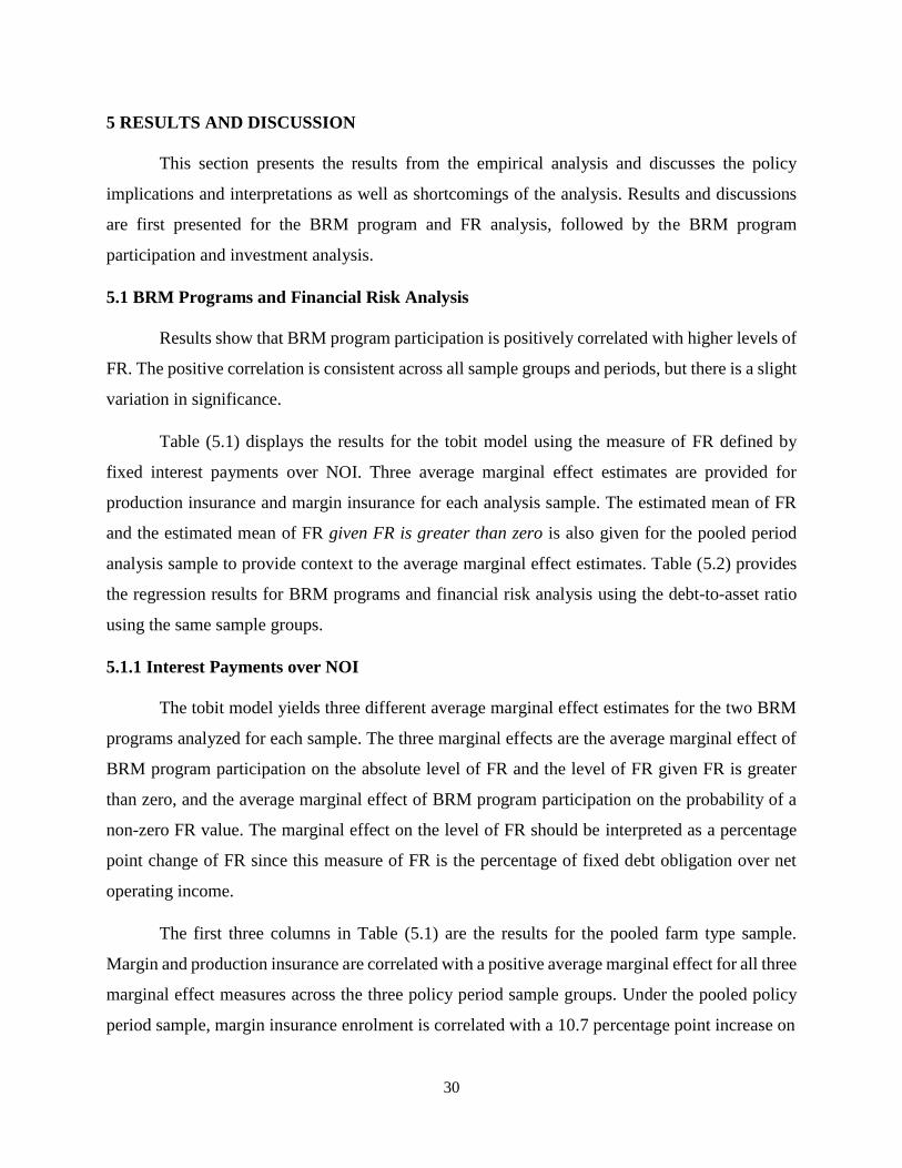
5 RESULTS AND DISCUSSION .............................................................................................. 30

5.1 BRM Programs and Financial Risk Analysis ...................................................................... 30

5.1.1 Interest Payments over NOI ......................................................................................... 30

5.1.2 Debt-to-Asset Ratio ...................................................................................................... 34

5.1.3 Summary of BRM Programs and Financial Risk Results ............................................ 34

5.1.4 Discussion ..................................................................................................................... 35

5.1.5 Limitations .................................................................................................................... 35

5.1.5.1 Endogeneity ........................................................................................................... 35

5.1.5.2 Interest Payments over NOI ................................................................................... 36

5.2 BRM Program Participation and Investment Analysis ....................................................... 36

5.2.1 Farm-Type Samples with FFS Investment Variable .................................................... 37

5.2.2 Alternative Capital Investment Variables..................................................................... 41

5.2.3 Discussion ..................................................................................................................... 42

5.2.3.1 Causal Relationship between BRM Program Participation and Investment ......... 42

5.2.3.2 BRM Programs Help Farms that Invest ................................................................. 43

5.2.3.3 Perceived Business Risk Reduction through BRM Programs ............................... 43

5.2.4 Limitations .................................................................................................................... 44

5.2.4.1 Observed Variables and Correlation ...................................................................... 44

5.2.4.2 Endogeneity ........................................................................................................... 44

5.3 Evaluating Results with respect to Policy Goals ................................................................. 45

6 CONCLUSION ........................................................................................................................ 47

REFERENCES ............................................................................................................................ 48

APPENDIX .................................................................................................................................. 51

vi

LIST OF TABLES

Table 4.1: Summary Statistics of Analysis Sample by Program Periods.................................. 19

Table 4.2: Summary Statistics of Farm Type Samples ............................................................. 21

Table 5.1: Results for Tobit Model using Fixed Debt Obligations FR Measure ...................... 31

Table 5.2: Results for Linear Regression Model using Debt-to-Asset Ratio FR Measure ....... 32

Table 5.3: BRM Program Participation and Investment Logit Results..................................... 38

Table 5.4: BRM Participation and Investment Logit Results with Alternative Investment

Variables .................................................................................................................. 39

Table A.1: Coefficients for Tobit Model using Fixed Debt Obligations FR Measure.............. 51

Table A.2: Coefficients for Linear Regression Model using Debt-to-Asset Ratio FR Measure

................................................................................................................................. 54

Table A.3: Coefficients for BRM Program Participation and Investment Logit ...................... 57

Table A.4: Coefficients for BRM Program Participation and Alternative Investment Variables

Logit ......................................................................................................................... 61

LIST OF FIGURES

Figure 2.1 Coverage and Payout Scheme for Margin Insurance Programs .................................... 5

vii

LIST OF ABBREVIATIONS

AME Average Marginal Effect

APF Agricultural Policy Framework

BR Business Risk

BRM Business Risk Management

GF Growing Forward

FR Financial Risk

1

1 INTRODUCTION

Business risk management (BRM) programs are important policy tools used to support the

Canadian agricultural industry. These programs are designed to mitigate the risk that is inherent in

agriculture through forms of yield insurance, margin insurance, and direct payments. While these

programs target risk associated with income variability, there have been many studies indicating

that there can be indirect effects of adjusting the risk faced by a farm business (e.g., Hennessey,

1998; O'Donoghue and Whitaker, 2010; Sckokai and Moro, 2009; Turvey, 2012). Altering the risk

profile of a business can affect operational behaviour and farm-level decisions.

A typical example of this is the moral hazard issue with insurance. Moral hazard occurs

when risk is reduced under insurance, and a firm alters their behavior as a result of the reduced

risk. In the context of agricultural BRM programs and farm operators, a particular risk is covered

under insurance which may incentivize the insured to increase or induce risk in another aspect of

their operation. If the adjustment of a risk-related behaviour is made given that it will raise their

expected well-being, profit, or another objective, then the adjustment in behaviour can be viewed

as optimizing with respect to the operations objective function. This concept has been generalized

into a framework called risk balancing (Gabriel and Baker, 1980; Collins, 1985). The general

theory states that the optimal level of different sources of risk faced by a firm will adjust with

respect to each other. In the context of BRM programs, it is important to consider the distinction

between moral hazard and optimization when discussing the context of farm-level behavioural

adjustments (Turvey, 2012).

Risk balancing can complicate the primary purpose of BRM programs: risk reduction. The

overall risk may not decrease if other risk components are adjusting in a manner that counters the

effects of the BRM program. That said, there may be positive adjustments that occur because of

or related to BRM program participation. The success or failure of BRM programs can be analyzed

by looking further into the factors that influence different types of risk, how the factors and risk

levels adjust, and if these outcomes are aligned with the stated policy goals.

This paper explores the relationship between BRM program enrollment and on-farm capital

investment behaviour of Canadian farms by examining the role of altering a farm operation’s risk

on their investment decision. The relationship between BRM programs and financial risk is also

2

examined. The risk balancing framework motivates analysis of these relationships. Previous

studies have examined risk balancing behaviour of farms but generally frame this behaviour in

negative contexts by commenting on changes in the overall likelihood of default (e.g., Featherstone

et al., 1988; Fernandez-Villaverde et al., 2011; Uzea et al., 2014; Vercammen, 2007). The literature

on agricultural insurance programs and farm-level decisions is also commonly framed in a negative

context such as examining the presence of moral hazard by looking at changes in input and output

decisions under insurance (Babcock and Hennessy, 1996; Ramaswami, 1993; Smith and Goodwin,

1996). Viewing investment as a risk-altering component shifts the focus of farm insurance and risk

balancing discussions away from negative behavioural adjustments towards potential productivity

gains through capital investment.

Evidence of a positive relationship between BRM program participation and investment is

found using a representative sample of Canadian farms obtained from the Farm Financial Survey

(FFS). A statistically significant positive correlation between the likelihood of investment and

BRM program enrolment is found across various policy periods and farm types. A statistically

significant positive correlation is found between BRM program enrolment and financial risk across

two measures of financial risk as well. The positive correlation between BRM program enrolment

and the likelihood of investment indicates that BRM programs may have indirect effects on risk-

related farm-level decisions such as investment. A possible interpretation of the results is that BRM

programs help operations that choose to invest; or more generally, farms that decide to invest may

also decide to enrol in BRM programs. Investment behaviour is an important factor in the growth

and productivity of agricultural operations. Evidence of the correlation between investment and

BRM programs highlights the importance for policymakers to take into consideration investment

behaviour when designing and evaluating agricultural programs.

The remainder of the paper begins with background on Canadian BRM programs and a

literature review of risk balancing theory, empirical applications of risk balancing, and investment

behaviour in Chapter 2. Chapter 3 provides an explanation of risk balancing theory using models

developed by Gabriel and Baker (1980) and Collins (1985) and the theory in the context of BRM

programs and investment. The empirical methodology is conducted in Chapter 4, followed by

results and discussion in Chapter 5. Chapter 6 concludes the paper with a summary and further

research suggestions.

3

2 BACKGROUND AND LITERATURE

This chapter is separated into three sections. The first section lays out the policy objectives

and technical design of the Canadian BRM programs examined in the analysis for this paper. The

second section reviews the theoretical interpretations and empirical application of risk balancing

theory in the literature. As the literature on risk and financial structure is extensive, papers and

empirical studies most relevant to the application in this paper are the focus of this section. The

final section summarizes the relevant literature on the effect of risk and risk-related factors on

investment behaviour and capital structure. This includes previous empirical literature examining

the relationship between investment and BRM programs.

2.1 BRM Programs in Canada

In recent decades, Canada's suite of BRM programs has been relatively stable. Under the

Canadian Agricultural Policy Framework (APF) spanning from 2003 to 2007, subsidized

production insurance and a form of margin insurance called the Canadian Agriculture Income

Stabilization (CAIS) program were a part of Canada's suite of BRM programs. Following APF,

the Growing Forward farm bill maintained the subsidized yield and margin insurance under the

titles AgriInsurance and AgriStability, respectively. The first Growing Forward spanned from

2008 to 2012. Growing Forward 2 maintained the suite of BRM programs under the same names

between 2013 and 2018. The level of coverage and margin reduction required to trigger a payment

has varied slightly, but the programs’ general designs have remained similar across the different

agricultural policy periods. Funding for the BRM programs across the APF and Growing Forward

policy periods are split 60:40 between the federal government and the provinces and territories

respectively.

2.1.1 Technical Details

The CAIS was a margin-based insurance. A payout occurred when the current year’s

allowable revenue less expenses was below the operation’s five-year Olympic average of that

measurement. This historical average is known as the reference margin. While 100% of an

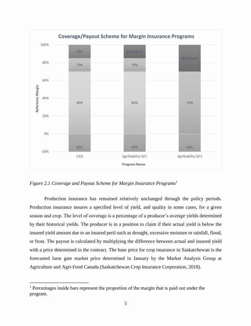
operation’s reference margin is covered, the level of payout depends on the margin of loss. A loss

of 0% to 15% triggered a 50% payout of that marginal loss. A loss of 15% to 30% triggered a 70%

payout of that marginal loss. A loss of 30% to 100% triggered an 80% payout of that marginal loss.

4

A negative margin, or loss greater than 100% of an operation’s reference margin, resulted in a 60%

payout on the negative margin.

BRM programs for Growing Forward 1 were launched in 2008. The new federal margin

insurance, AgriStability, applied the same use of a reference margin as in CAIS. AgriStability

provided coverage for 85% of an operation’s reference margin, unlike CAIS which covered 100%.

In Growing Forward, the upper portion of coverage was replaced by AgriInvest which allowed

farmers to place up to 100% of their net allowable sale in an account wherein the government

matched 1% of the farmer’s contributions, up to $15,000. Under AgriStability, a loss between 15%

and 30% triggered a 70% payout of that marginal loss. A loss of 30% to 100% triggered an 80%

payout of that marginal loss. A loss of greater than 100% of the reference margin triggered a 60%

payout of the negative margin.

Growing Forward 2 was implemented in 2013 and made only minor changes to the

previous suite of BRM programs. This iteration of AgriStability covered 70% of an operation's

reference margin. AgriInvest remained intact with its intended purpose of covering small marginal

declines. Changes were made to how the reference margin was calculated, such as widening the

scope of allowable revenue and expenses. A significant change to the program was the use of an

operation’s allowable expenses as their program reference margin if this value was lower than the

traditional reference margin calculation. This decreased coverage for operations with low input

costs relative to their reference margin. A loss of 30% to 100% triggered a 70% payout of that

marginal loss. A negative margin results in a 60% payout of that marginal loss. Figure (1) gives a

visual depiction of the coverage provided by CAIS and AgriStability from Growing Forward 1

and 2.

5

Figure 2.1 Coverage and Payout Scheme for Margin Insurance Programs1

Production insurance has remained relatively unchanged through the policy periods.

Production insurance insures a specified level of yield, and quality in some cases, for a given

season and crop. The level of coverage is a percentage of a producer’s average yields determined

by their historical yields. The producer is in a position to claim if their actual yield is below the

insured yield amount due to an insured peril such as drought, excessive moisture or rainfall, flood,

or frost. The payout is calculated by multiplying the difference between actual and insured yield

with a price determined in the contract. The base price for crop insurance in Saskatchewan is the

forecasted farm gate market price determined in January by the Market Analysis Group at

Agriculture and Agri-Food Canada (Saskatchewan Crop Insurance Corporation, 2018).

1 Percentages inside bars represent the proportion of the margin that is paid out under the

program.

80% 80%

70% 70%

70%

60% 60% 60%

50% No Payout

No Payout

-20%

0%

20%

40%

60%

80%

100%

CAIS AgriStability GF1 AgriStability GF2

Re

fere

nce

Mar

gin

Program Name

Coverage/Payout Scheme for Margin Insurance Programs

6

The primary objective of covering a specified level of quantity or quality of production is

carried throughout APF and Growing Forward 1 and 2. The level of coverage, price options, and

other program parameters can vary across provinces and individuals within provinces, even within

policy periods. Although the cost of government production insurance is jointly shared between

the federal and the provincial and territorial levels of government, the provinces are responsible

for administering production insurance.

2.1.2 Policy Goals

There are two types of policy goals to look at when evaluating BRM programs. The first is

the policy directives for the overarching agricultural policy framework (i.e., APF and Growing

Forward). The second is the policy goals for the individual BRM programs. While each program

has a primary purpose, some are suffixed by supplementary goals and general principles that

dictate the function and application of the program (Agriculture and Agri-Food Canada, 2005;

Agriculture and Agri-Food Canada, 2008).

A 2005 APF federal-provincial-territorial agreement states the objectives of the policy

framework as positioning Canada to be a global leader in food safety, innovation, and

environmentally-responsible production. Farm-level investment can play an important role in each

of these objectives.

The desired strategic outcomes for Growing Forward are laid out in a federal-provincial-

territorial agreement as the following: “a sector that is proactive in managing risk, a sector that

contributes to society’s priorities, and a competitive and innovative sector” (Agriculture and Agri-

Food Canada, 2008). The first point refers directly to BRM programs and their primary goal of

managing risk. The third point can be interpreted as promoting investment by farms which

facilitate the adoption of innovative technologies and practices. The third point is reiterated in the

agreement in a section stating the general principles of risk management programming. It states

that BRM programs “should contribute to market-oriented adjustments and adoption of

technological innovations” (Agriculture and Agri-Food Canada, 2008).

The general principles of risk management programming also state that “programs should

minimize moral hazard and not influence farmers’ production and marketing decisions”

(Agriculture and Agri-Food Canada, 2008). The interpretation of moral hazard likely refers to

7

decisions related to the risk that is covered under the program. For example, if a farmer has yield

insurance for canola, but not other crops, he may decide to plant a higher proportion of canola,

reducing the diversity of his operation and increasing the risk and probability of payout.

Alternatively, if the moral hazard problem is viewed in a whole farm perspective, the adjustment

of risky behaviour could occur in another aspect of the farm business not directly related to current

canola yields such as investment or financing decisions.

The same document states that “payments for the purpose of stabilization, disaster

mitigation or production loss should not be capitalized into assets” (Agriculture and Agri-Food

Canada, 2008). Capitalization of assets is seen with Common Agricultural Policy payments and

land prices in Europe, where direct farm payments caused farmland prices to inflate (Guastella et

al., 2018; Kirwan and Roberts, 2016; O’Neill and Hanrahan, 2016). A less direct form of

capitalization of program payments may occur through increased productivity. Program payments

may influence farmers’ behaviour in a way that results in increased productivity. The increased

productivity may then be capitalized into farm assets.

Across both APF and Growing Forward policy periods, the primary policy goal for BRM

programs was to provide agricultural producers with tools to manage risk and stabilize farm

incomes. Income stabilization programs like CAIS and AgriStability targeted whole farm incomes

and aimed to provide support for large margin losses. Production insurance under APF and

AgriInsurance were designed to stabilize farmers' incomes by minimizing the financial impact of

production losses due to natural causes.

2.2 Risk Balancing

The theory of risk balancing was formalized in a paper by Gabriel and Baker (1980). The

risk balancing framework is presented as an equation representing the total risk faced by a firm as

the combination of financial risk and business risk constrained by the “maximum tolerable total

risk.” How this tolerable level of total risk is calculated is not explicitly stated in the paper but is

assumed to be determined when optimizing profit subject to total risk.

Collins (1985) presents an alternative model that is consistent with the risk balancing

framework put forward by Gabriel and Baker (1980). Collins suggests a structural model of the

8

debt-equity decision faced by a firm. Maximizing the equation provides us with relationships

between different components of risk that are found in Gabriel and Baker’s model.

Featherstone et al. (1988) develop a theoretical framework of risk balancing by

constructing a mean-variance model to determine the optimal leverage for a firm. Comparative

statistic analysis carried out on the model provides results consistent with the previous risk

balancing literature. Featherstone et al. (1988) find that policies aimed at reducing the variability

of return on assets, or business risk, increase the variance of return on equity through increased

leverage, or financial risk. They find that business risk-reducing policies increase the probability

of a firm losing all or part of their equity capital and going bankrupt due to the increase in optimal

leverage.

The common approach to empirical risk balancing analysis is through correlation analysis

and regression analysis with panel data to estimate adjustments in risk measures across time.

Several empirical papers approach risk balancing directly by examining business risk and financial

risk explicitly, while others provide evidence of risk balancing though specific farm-level

behavioural adjustments. Escalante and Barry (2003) approach risk balancing directly by

conducting correlation analysis on business and financial risk measures for a sample panel of

Illinois grain farmers. They find that risk balancing is most evident when using a business risk

measure that only accounts for the previous two years. De Mey et al. (2014) and Uzea et al. (2014)

apply correlation and regression analysis on a panel of farms from the EU-15 and Ontario, Canada,

respectively. De Mey et al. (2014) find evidence of risk balancing through both methods with

regression results showing that financial risk adjusts following a change in business risk. Uzea et

al. (2014) find just over half their sample displays risk balancing behaviour, but their regressions

results find no evidence of year-over-year financial risk adjustment.

Of the papers that touch on risk balancing implicitly, there are several that examine how

risk-related agricultural programs and policies affect risk-related farm behaviour. Coble et al.

(2000) examine how crop and revenue insurance affect the level of hedging for US corn producers,

where hedging can be seen as an alternative risk management tool. They find that crop insurance

is complementary to hedging while pure revenue insurance has a strong substitution effect and

therefore reduces the demand for hedging. Turvey (2012) looks at the optimal crop choice faced

by a representative sample of Manitoba producers under whole farm revenue insurance. Using

9

simulated data, Turvey (2012) finds that whole farm income insurance with subsidised premiums

can affect producers' choice of crops. Uzea et al. (2014) and Ifft et al. (2015) look at the effect of

insurance on the different measures of financial risk. Uzea et al. (2014) find enrolment in federal

margin insurance programs to be correlated with an increase in financial risk, measured by interest

expenses over total operating revenue, for crop and beef producers. Ifft et al. (2015) use propensity

score matching on a representative sample of US farms to estimate the difference in debt levels for

operations that participate in federal crop insurance programs and those that do not. They find

federal crop insurance program participation to be correlated with short-term farm debt, but not

long-term farm debt. These empirical studies allude to risk balancing behaviour as they find that

participation in risk-reducing programs like insurance may lead to adjustments in risk-related farm

behaviour such as the use of risk-reducing tools or the decision to take on more debt.

2.3 Investment Decision and Risk

Investment under uncertainty is a well-researched topic with many studies examining the

adverse effects of uncertainty on investment behaviour (e.g., Baum et al., 2010; Bloom et al. 2007;

Boyle and Guthrie, 2003; Doshi et al., 2017; Fernandez-Villaverde et al., 2011). While there is a

vast literature on investment and uncertainty, the focus of this section is to review literature that is

relevant to the agricultural industry. Empirical studies of farm investment behaviour are reviewed

to guide the methodology and motivate the risk balancing relationship between BRM program

enrolment and investment.

Uncertainty can stem from policy, interest rates, rate of return, and cash flow, all of which

can affect investment. The effect of uncertainty on investment behaviour can be ambiguous if the

source of uncertainty is not specified (e.g., Baum et al., 2010; Boyle and Guthrie, 2003). Baum et

al. (2010) look at the US manufacturing sector and examine the linkages between uncertainty

derived from a firm's stock return, overall market uncertainty, and capital investment behaviour.

Their results show that uncertainty or volatility in the market has a direct negative effect on fixed

capital investment spending. They also find that uncertainty derived from a firm's own returns

effects investment through cash flow, while the sign of the effect may vary. Caballero and Pindyck

(1996) use the firm-level US to find higher industry-wide uncertainty, defined by the variance of

the marginal revenue product of capital, raises the required rate of return on capital for an

investment to occur. Ghosal and Loungani (2000) use industry-level data to find that uncertainty

10

of profits for US firms decreases expenditure on investment, with the negative effect on investment

more substantial for industries consisting of smaller firms.

There are several recent empirical studies examining investment behaviour and income

stabilizing agriculture programs. Heikkinen and Pietol (2009) model optimal investment behaviour

and cost of uncertainty using a dynamic stochastic programming model. They find that uncertainty

costs are dependant on future income variability, therefore affecting the decision to invest, as well

as timing. In some cases, greater future income variability is found to increase an option value of

postponing an investment. Their analysis is motivated by cases of policy uncertainty causing the

rate of return of investment to be uncertain for Finnish farmers.

Sckokai and Moro (2009) apply a dynamic dual model of choice under uncertainty,

allowing for farmers' risk attitudes, to evaluate the effect of Common Agricultural Policy (CAP)

BRM programs on farm investment behaviour. A dataset of Italian crop farmers is used to

parameterise a normalised quadratic multi-period expected utility function. The resulting

investment demand equation and supply equations are then used to simulate the effect of different

policies on the demand for investment. They find that farm investment is positively affected by

price intervention policies due to reduced price volatility. Policies unrelated to output price

uncertainty have a smaller effect on investment behaviour. Their results show that uncertainty

surrounding expected profit, and thus policies that effect uncertainty, can affect investment

behaviour.

Kallas et al. (2012) use a reduced-form application of the model by Sckokai and Moro

(2009) to evaluate the effect of CAP direct payment programs based on historical yields on

investment behaviour. The model is applied to a dataset of cereal, oilseed, and protein producers

in Spain. They find evidence that program payments affect investment decision positively for

buildings, land improvements, machinery, and equipment. Their analysis also finds crop insurance

contracts increase investment through its reduction in revenue uncertainty.

Investment can be affected by financial constraints or credit accessibility which, in turn,

can be closely linked to risk faced by agricultural operations. Minton and Schrand (1999) find cash

flow volatility to increase the cost and likelihood of accessing capital markets for US firms using

firm-level data. Their results suggest that firms forgo investment rather than access external capital

markets to cover cash flow deficits. Hughes et al. (1984) estimate the effect of federal credit

11

subsidies on the financial structure and investment behaviour of US farms. Simulations are

conducted using a baseline model which is estimated using 1976 to 1980 data. They find a small

decrease in farm debt in the short-term and a larger decrease in the long-term with a marginal

reduction in farm credit subsidies. Hughes et al. also find that the absence of federal credit

subsidies translates to farmers holding fewer financial assets and owing less debt as a result. In

other words, greater access to credit may result in more financial assets, but higher debt. Empirical

studies have found agricultural investment to be affected by financial constraints by looking at the

sensitivity of investment to cash-flow as a measure of financial constraints (e.g., Benjamin and

Phimister, 2002; Bierlen and Featherstone, 1998; Chaddad et al., 2005). O’Toole et al. (2014) find

similar results in the context of the Irish financial crisis using a measure of internal financial

dependence versus external financing as a determinant of financial constraints due to criticisms of

the cash-flow measure. These results imply that credit accessibility can influence investment and

the level of financial risk of an agricultural operation.

12

3 THEORETICAL MODEL

3.1 Risk Balancing Model

This paper will rely on the theoretical models presented by Gabriel and Baker (1980) and

Collins (1985). Gabriel and Baker (1980) provide a simple understanding of risk balancing

behaviour using a risk constraint, while Collins (1985) represents risk balancing in a structural

equation of the debt-equity decision made by the farm business to maximize the expected utility

of wealth. Both approaches yield results that are consistent with the hypothesized positive

relationship between BRM program enrolment and investment but provide different interpretations

of risk measures.

The total risk a business faces can be separated into the two distinct components of business

risk (BR) and financial risk (FR). Gabriel and Baker (1980) define BR as the inherent risk in the

farms operating performance, independent of how it is financed. The risk associated with weather

or commodity prices are typical examples of BR in agriculture. FR is defined as the added risk

associated with how an operation finances its debt. Interest rate risk, credit risk, and other risks

associated with leverage fall under FR. For example, if an operation's fixed debt obligations

increase due to movements in interest rates, FR has increased.

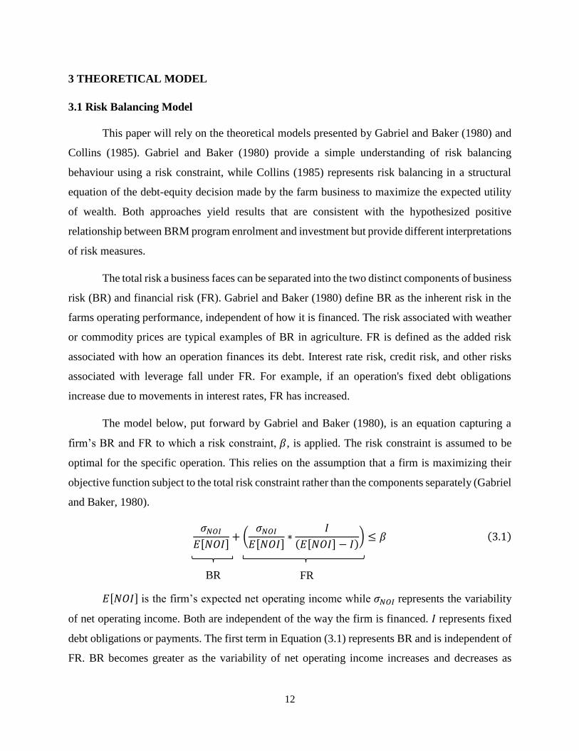
The model below, put forward by Gabriel and Baker (1980), is an equation capturing a

firm’s BR and FR to which a risk constraint, 𝛽, is applied. The risk constraint is assumed to be

optimal for the specific operation. This relies on the assumption that a firm is maximizing their

objective function subject to the total risk constraint rather than the components separately (Gabriel

and Baker, 1980).

𝜎𝑁𝑂𝐼

𝐸[𝑁𝑂𝐼]+ (

𝜎𝑁𝑂𝐼

𝐸[𝑁𝑂𝐼]∗

𝐼

(𝐸[𝑁𝑂𝐼] − 𝐼)) ≤ 𝛽 (3.1)

𝐸[𝑁𝑂𝐼] is the firm’s expected net operating income while 𝜎𝑁𝑂𝐼 represents the variability

of net operating income. Both are independent of the way the firm is financed. 𝐼 represents fixed

debt obligations or payments. The first term in Equation (3.1) represents BR and is independent of

FR. BR becomes greater as the variability of net operating income increases and decreases as

BR FR

13

expected net operating income increases. The second term in brackets represents FR, defined as

the interaction between 𝐼

(𝐸[𝑁𝑂𝐼]−𝐼) and

𝜎𝑁𝑂𝐼

𝐸[𝑁𝑂𝐼]. FR can be interpreted as the added risk to an

operation’s net operating income due to fixed debt obligations. As fixed debt obligations increase,

so does FR. In this model, it is not clear whether fixed debt obligations increase due to higher debt

or interest rates. FR also increases with increased BR.

The risk balancing behaviour occurs through the strategic adjustment of FR and BR

components to maintain the optimal level of total risk or 𝛽. Consider the case of an exogenous

reduction in 𝜎𝑁𝑂𝐼 due to policy. A decrease in 𝜎𝑁𝑂𝐼 reduces the first BR term as well as decreasing

the FR term through a reduction in BR. There is now slack in the risk constraint, allowing

adjustments in FR or BR through firm-level adjustments to increase total risk back to the optimal

level, 𝛽.

The risk balancing model by Collins (1985) specifies a structural equation that maximizes

an operation's expected utility of the rate of return on equity with respect to their debt-to-asset ratio.

The fundamental assumption of Collins' model is that a farm's primary objective is to maximize

their expected utility of the rate of return on equity. Collins refers to BR as the variance or rate of

return on assets. Like Gabriel and Baker (1980), FR is the added variability to the return on equity

stemming from the operation’s leverage position. Below is the debt-equity decision,

max𝛿

𝐸𝑈[𝑅𝑂𝐸] = 𝐸[𝑅𝑂𝐸] −𝜌

2𝜎𝑅𝑂𝐸

2 (3.2)

where 𝐸[𝑅𝑂𝐸] is the expected rate of return on equity, 𝜌 is a risk aversion parameter, and 𝜎𝑅𝑂𝐸2 is

the variance of the rate of return on equity. 𝐸[𝑅𝑂𝐸] is assumed to be a function of the expected

rate of return on assets (𝐸[𝑅𝑂𝐴]), the fixed interest rate on debt (𝑖), and the debt-to-asset ratio (𝛿)

as defined below.

𝑅𝑂𝐸 = (𝑅𝑂𝐴 − 𝑖𝛿)(1 − 𝛿)−1

𝐸[𝑅𝑂𝐸] = (𝐸[𝑅𝑂𝐴] − 𝑖𝛿)(1 − 𝛿)−1 (3.3)

𝜎𝑅𝑂𝐸2 = 𝜎𝑅𝑂𝐴

2 (1 − 𝛿)−2 (3.4)

14

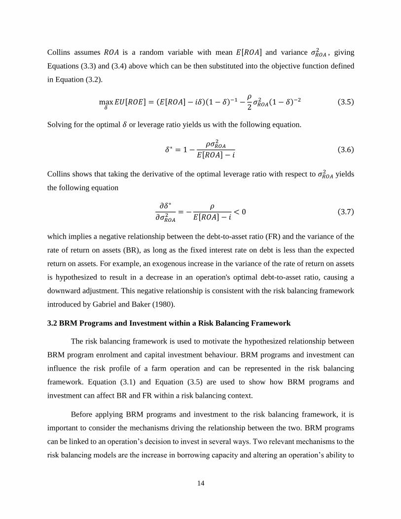
Collins assumes 𝑅𝑂𝐴 is a random variable with mean 𝐸[𝑅𝑂𝐴] and variance 𝜎𝑅𝑂𝐴2 , giving

Equations (3.3) and (3.4) above which can be then substituted into the objective function defined

in Equation (3.2).

max𝛿

𝐸𝑈[𝑅𝑂𝐸] = (𝐸[𝑅𝑂𝐴] − 𝑖𝛿)(1 − 𝛿)−1 −𝜌

2𝜎𝑅𝑂𝐴

2 (1 − 𝛿)−2 (3.5)

Solving for the optimal 𝛿 or leverage ratio yields us with the following equation.

𝛿∗ = 1 −𝜌𝜎𝑅𝑂𝐴

2

𝐸[𝑅𝑂𝐴] − 𝑖(3.6)

Collins shows that taking the derivative of the optimal leverage ratio with respect to 𝜎𝑅𝑂𝐴2 yields

the following equation

𝜕𝛿∗

𝜕𝜎𝑅𝑂𝐴2 = −

𝜌

𝐸[𝑅𝑂𝐴] − 𝑖< 0 (3.7)

which implies a negative relationship between the debt-to-asset ratio (FR) and the variance of the

rate of return on assets (BR), as long as the fixed interest rate on debt is less than the expected

return on assets. For example, an exogenous increase in the variance of the rate of return on assets

is hypothesized to result in a decrease in an operation's optimal debt-to-asset ratio, causing a

downward adjustment. This negative relationship is consistent with the risk balancing framework

introduced by Gabriel and Baker (1980).

3.2 BRM Programs and Investment within a Risk Balancing Framework

The risk balancing framework is used to motivate the hypothesized relationship between

BRM program enrolment and capital investment behaviour. BRM programs and investment can

influence the risk profile of a farm operation and can be represented in the risk balancing

framework. Equation (3.1) and Equation (3.5) are used to show how BRM programs and

investment can affect BR and FR within a risk balancing context.

Before applying BRM programs and investment to the risk balancing framework, it is

important to consider the mechanisms driving the relationship between the two. BRM programs

can be linked to an operation’s decision to invest in several ways. Two relevant mechanisms to the

risk balancing models are the increase in borrowing capacity and altering an operation’s ability to

15

finance debt resulting from the investment. Enrolment in BRM programs may signal to potential

creditors good business planning and management abilities, and therefore a reduced risk of

defaulting on their loan. BRM program enrolment can increase the amount and likelihood of credit

available for an operation to make an investment (Hughes et al., 1984; Minton and Schrand, 1999).

BRM programs can also increase an operation's ability to finance their debt by reducing the

volatility of cash flow, providing an operation with consistent cash flow necessary to finance debt.

BRM programs and investment have a positive relationship through both these mechanisms.

Under the model presented by Gabriel and Baker (1980), both program participation and

investment can alter components of Equation (3.1). The design of BRM programs is to reduce

income volatility faced by farmers. Given this, program participation should reduce 𝜎𝑁𝑂𝐼 within

the model. This reduces the BR component and part of the FR component, resulting in a reduction

of total risk. Investment can increase 𝐼 within the FR component if investments are made through

debt, therefore increasing the fixed debt obligations. By increasing 𝐼 through investment, FR

increases, resulting in an increase of total risk. In Equation (3.1), BRM program participation and

investment have opposite effects on the level of total risk. Investment and BRM program

participation have a positive relationship within the model presented by Gabriel and Baker (1980).

The model developed by Collins (1985) has a similar result. In Equation (3.5), BRM

program participation should reduce the variability of the rate of return on assets (𝜎𝑅𝑂𝐴2 ), while

investments made through debt financing will affect the debt-to-asset ratio (𝛿). Equation (3.7)

shows that the optimal 𝛿 and 𝜎𝑅𝑂𝐴2 are negatively correlated. Therefore, a decrease in 𝜎𝑅𝑂𝐴

2 , or BR,

through BRM program enrolment translates to an increase in the optimal 𝛿, or FR.

Risk balancing theory provides a basic model to explicitly show the intuitive, positive

relationship between BRM program participation and investment behaviour, while the

mechanisms driving the relationship are not made explicit in the models. The uncertainty of the

mechanisms is addressed in the discussions section for the BRM program and investment analysis

in Chapter 5.

16

4 EMPIRICAL METHODOLOGY

The empirical analysis is divided into three sections. First, summary statistics for the data

are presented. Second, regression analysis is conducted to examine the relationship between BRM

program participation and financial risk measures. Third, the relationship between BRM program

participation and investment is empirically examined.

The analysis is carried out across pooled samples as well as different sub-samples

distinguished by policy period and farm type. Production insurance and margin insurance

participation enter the models simultaneously but separately as farms can choose to participate in

one, both, or neither of the programs.

The analysis is applied to grain and oilseed producers, cattle operations, and a pooled

sample. Each farm type sample, including the pooled sample, is further separated and analyzed by

policy period. Grain and oilseed producers and cattle operations are separately examined because

they constitute a large proportion of Canada's agricultural industry. It is also likely that different

BRM programs will have varying effects on different operation types. For example, crop insurance

is tailored for certain types of crop producers while margin insurance such as AgriStability is

designed for a wider variety of operations.

4.1 Data

The data used for the two analysis sections is survey data from the Farm Financial Survey

(FFS) provided through Agriculture and Agri-Food Canada. The FFS provides financial data on a

representative sample of Canadian farms across different types of agricultural operations. The data

includes assets, liabilities, revenues, costs, capital sales, capital investments, and farm

characteristics for each survey reference year. The reference year is either the fiscal year or

calendar year depending on how an operation records its information.

Available data spans from 1999 to 2015 with gaps due to changing frequency of the survey

across the period. The period of data used for analysis spans from 2003 to 2015. During this period,

the survey was conducted annually from 2003 to 2011, then every two years from 2011 to 2015.

Financial data necessary for constructing variables for the BRM program and investment analysis

is not collected for survey years 2006, 2008 and 2010. The data can be divided into two policy

17

periods. The first policy period covers the APF from 2003 to 2007 while the second policy periods

covers Growing Forward 1 and 2 from 2008 to 2015.

The analysis of the paper focuses on the two primary forms of BRM programs, government

subsidized production and margin insurance, from 2003 to 2015. Private insurance alternatives to

these BRM programs are available during this period but are not used in the analysis. This is due

to the lack of data on private insurance enrolment and the relatively small market share these

private options hold. AgriInvest is not examined in the analysis due to its high rate of enrolment

in the sample. In other words, there is little variation in participation. With respect to risk

management, part of the stated objective of AgriInvest is to help farms manage small income

declines by encouraging them to save and receive payment for doing so (Agriculture and Agri-

Food Canada, 2018). The amount of direct payment is capped at $15,000 per program year. This

is a relatively small amount of relief in the event of a margin decline and would likely not have a

large effect on risk related behaviour.

A new representative sample is drawn each survey year resulting in a repeated cross-

sectional dataset. There is a roughly 30 percent overlap of survey respondents year over year, but

they cannot be tracked across more than two survey years. The survey sample pulls farms from

the Business Register to obtain a list of all farms in Canada. These farms are placed into a stratum

based on province, size, and type of operation. The size of each stratum is determined by the

revenue and assets of the farms. Simple random sample takes place at the stratum level. Sampling

weights are applied to each farm in the sample based on the probability of selection. These weights

are used for obtaining summary statistics of the sample and estimating models in the analysis

section. Since this is a representative sample of Canadian farms, the composition of farms in the

sample reflect the composition of the farm population.

In 2013, farms with less than $25,000 in farm revenue were excluded from the sampling

population. Farm operations in previous sample years with less than $25,000 are dropped to

maintain a consistent sample group across survey years.

4.1.1 Descriptive Statistics

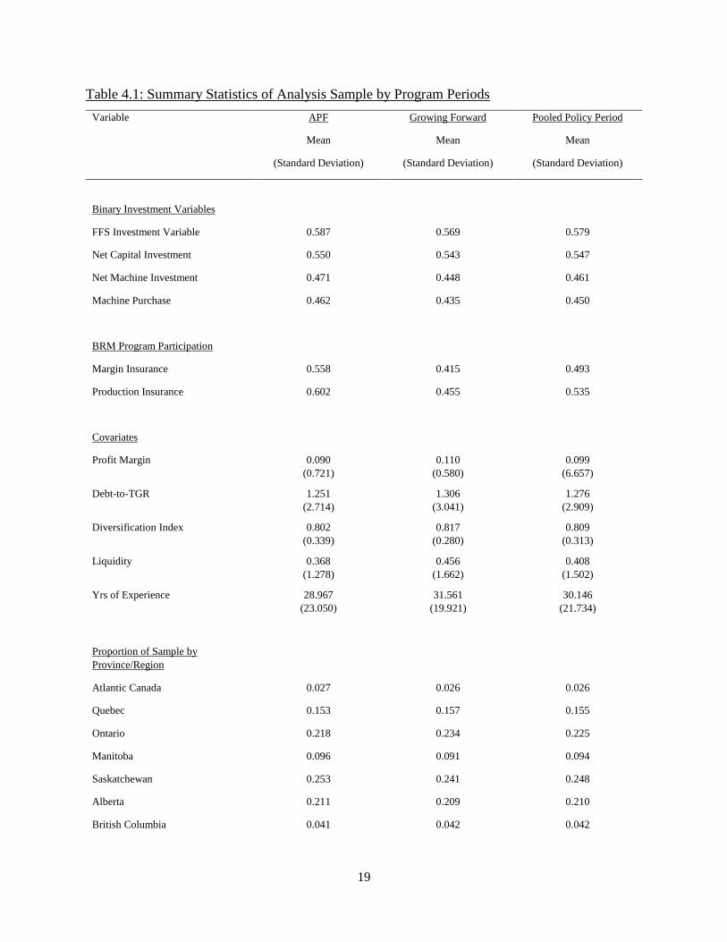
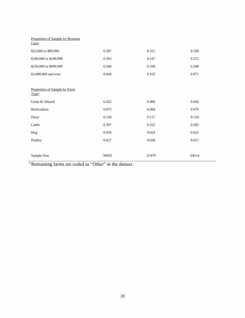
Table (4.1) provides descriptive statistics of the pooled sample used in the BRM program and

investment analysis for the variables defined above. Descriptive statistics are given for each policy

18

period. The descriptive statistics apply to the total population of Canadian agricultural operations

with the use of probability weights. The mean and standard deviation for each variable is estimated.

The descriptive statistics of the analysis sample reflect statistics for the Canadian agriculture

industry released by Statistics Canada across the sample years.1 This indicates that our sample is

representative of Canadian farms.

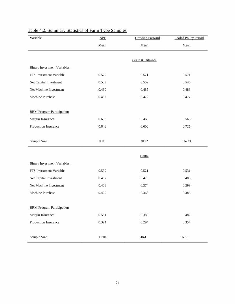
Table (4.2) provides the weighted means of the investment variables and BRM program

enrolment for grain and oilseed producers and cattle operations by policy periods. BRM program

enrolment rates for the APF consistent with program assessment reports published by AAFC,

while enrolment rates during the Growing Forward policy period are slightly lower than figures

released by AAFC for both farm types. The general reduction in enrolment between policy periods

is consistent with the published rates.

While investment rates between policy periods for grain and oilseed producers are

relatively unchanged, there are notable differences between policy periods for cattle operations.

The proportion of cattle operations making an investment based on the FFS variable decreases by

roughly 18 percentage points from APF to Growing Forward. There is also a decrease of about 10

percentage points for the net capital investment variable, 3 percentage points for the net machine

investment variables, and 4.5 percentage points for the machine purchase variable.

4.2 BRM Program Participation and Financial Risk

Before analyzing the relationship between BRM programs and investment, the question of

whether BRM program participation is correlated with higher FR is examined. While the

relationship between BRM program participation and FR is motivated by risk balancing theory, it

cannot directly represent a risk balancing relationship because BRM program participation may

not necessarily translate to lower BR. The hypothesized positive relationship between BRM

program participation and FR provides important context for understanding the BRM program

participation and investment relationship. Two measures of FR requiring separate empirical

approaches are used in the analysis. The use of two FR measures is applied for robustness.

1 Farms classified by farm type, historical data. Table: 32-10-0166-01. Statistics Canada

Farms classified by size, historical data. Table: 32-10-0156-01. Statistics Canada

Farms classified by total gross farm receipts, 2015 constant dollars, historical data. Table: 32-

10-0157. Statistics Canada

19

Table 4.1: Summary Statistics of Analysis Sample by Program Periods

Variable APF Growing Forward Pooled Policy Period

Mean

(Standard Deviation)

Mean


Mean


Binary Investment Variables

FFS Investment Variable 0.587 0.569 0.579

Net Capital Investment 0.550 0.543 0.547

Net Machine Investment 0.471 0.448 0.461

Machine Purchase 0.462 0.435 0.450

BRM Program Participation

Margin Insurance 0.558 0.415 0.493

Production Insurance 0.602 0.455 0.535

Covariates

Profit Margin 0.090

(0.721)

0.110

(0.580)

0.099

(6.657)

Debt-to-TGR 1.251

(2.714)

1.306

(3.041)

1.276

(2.909)

Diversification Index 0.802

(0.339)

0.817

(0.280)

0.809

(0.313)

Liquidity 0.368

(1.278)

0.456

(1.662)

0.408

(1.502)

Yrs of Experience 28.967

(23.050)

31.561

(19.921)

30.146

(21.734)

Proportion of Sample by

Province/Region

Atlantic Canada 0.027 0.026 0.026

Quebec 0.153 0.157 0.155

Ontario 0.218 0.234 0.225

Manitoba 0.096 0.091 0.094

Saskatchewan 0.253 0.241 0.248

Alberta 0.211 0.209 0.210

British Columbia 0.041 0.042 0.042

20

Proportion of Sample by Revenue

Class

$25,000 to $99,999 0.397 0.312 0.358

$100,000 to $249,999 0.293 0.247 0.272

$250,000 to $999,999 0.266 0.338 0.298

$1,000,000 and over 0.044 0.103 0.071

Proportion of Sample by Farm

Typea

Grain & Oilseed 0.422 0.496 0.456

Horticulture 0.075 0.084 0.079

Dairy 0.130 0.117 0.124

Cattle 0.307 0.252 0.282

Hog 0.039 0.024 0.032

Poultry 0.027 0.028 0.027

Sample Size 39035 25479 64514

a Remaining farms are coded as “Other” in the dataset.

21

Table 4.2: Summary Statistics of Farm Type Samples

Variable APF Growing Forward Pooled Policy Period

Mean Mean Mean

Grain & Oilseeds









Sample Size 8601 8122 16723

Cattle









Sample Size 11910 5041 16951

22

The first approach uses 𝐼

(𝑁𝑂𝐼−𝐼), the percentage of fixed interest payments over net-

operation-income, as a measure of FR. This measure is consistent with the model by Gabriel and

Baker (1980) and is used in previous empirical risk balancing analysis (De Mey et al., 2014; Uzea

et al., 2014). To reiterate, 𝐼 is the operation's fixed interest payments or fixed debt obligations in

the model. (𝑁𝑂𝐼 − 𝐼) is the operation’s net operating income less fixed interest payments. By

dividing the fixed interest payments by net-operating-income, the FR measure becomes a risk

index that can be compared across farm sizes. A greater 𝐼 or lower 𝑁𝑂𝐼 results in a higher FR level.

This measure of FR results in farms being dropped from the sample due to zero and negative net-

operating-income values. The implications of the dropped observations on our results are touched

on in the shortcomings section for the BRM program and FR analysis in Chapter 5. Many farms

do not have any fixed interest payments resulting in a clustering around zero.

Using the fixed interest payments measure of FR, a tobit model is applied due to the large

number of FR values, the dependent variable, equal to zero. A tobit models the effect of the

explanatory variables on the dependent variable at the extensive and intensive margin separately.

In this case, the extensive margin is whether an operation has a zero value of FR or a value greater

than zero, while the intensive margin looks at the change in the amount of FR. The tobit model

estimates the effect of BRM program enrolment on both these margins.

The tobit model is defined by the following two assumptions.

𝑦 = max(0, 𝑋𝛽 + 𝑢) (4.1)

𝑢|𝑋~𝑁(0, 𝜎2) (4.2)

Equation (4.1) states that the dependent variable 𝑦, or FR, is a maximum of zero or a

positive value defined by 𝑋𝛽 + 𝑢, where 𝑋 are explanatory covariates, 𝛽 is a vector of coefficients,

and 𝑢 is the unobserved error term. The zero-value corner solution reflects the distribution of FR

using fixed interest payments over net-operation-income in the data. Equation (4.2) states that the

distribution of the error term in Equation (4.1) is normally distributed with mean zero and some

variance.

The density function of a tobit is defined in Equation (4.3) below. The first and second

term on the righthand side of the equation represent the density of the intensive and extensive

23

margin respectively. The exponent of each term is an indicator function that is equal to 1 when the

statement inside the square brackets is true, thus separating the density of FR by zero and non-zero

values. Θ is the normal cumulative distribution function, while 𝜃 is the normal probability density

function.

𝑓(𝐹𝑅|𝑋) = {Θ [𝑋𝛽

𝜎] 𝜎−1

𝜃 [𝐹𝑅 − 𝑋𝛽

𝜎 ]

Θ [𝑋𝛽𝜎 ]

}

1[𝐹𝑅>0]

∗ {1 − Θ [𝑋𝛽

𝜎]}

1[𝐹𝑅=0]

(4.3𝑎)

The density of the tobit is represented in Equation (4.3a). The binary component of the tobit model

is made up of Θ [𝑋𝛽

𝜎] in the first term, representing the probability of a non-zero value of FR, and

the entire second term, 1 − Θ [𝑋𝛽

𝜎], representing the probability of FR equal to zero. These address

the extensive margin. The uncensored linear section of the tobit is modeled by 𝜎−1𝜃[

𝐹𝑅−𝑋𝛽

𝜎]

Θ[𝑋𝛽

𝜎]

,

representing the probability density of FR greater than zero. This addresses the intensive margin.

Equation (4.3a) simplifies to Equation (4.3b).

𝑓(𝐹𝑅|𝑋) = {𝜎−1𝜃 [𝐹𝑅 − 𝑋𝛽

𝜎]}

1[𝐹𝑅>0]

∗ {1 − Θ [𝑋𝛽

𝜎]}

1[𝐹𝑅=0]

(4.3𝑏)

A sample log-likelihood expression can be derived from the density function to give us Equation

(4.4) below.

ℓ𝑖(𝛽, 𝜎) = 1[𝐹𝑅𝑖 > 0] (𝑙𝑛 {𝜃 [𝐹𝑅𝑖−𝑋𝑖𝛽

𝜎]} −

𝑙𝑛(𝜎2)

2) + 1[𝐹𝑅𝑖 = 0]𝑙𝑛 {1 − Θ [

𝑋𝑖𝛽

𝜎]} (4.4)

This can be rewritten as

ℓ𝑖(𝛽, 𝜎) = 1[𝐹𝑅𝑖 = 0]𝑙𝑛 {1 − Θ [𝑋𝑖𝛽

𝜎]} − 1[𝐹𝑅𝑖 > 0] {

(𝐹𝑅𝑖 − 𝑋𝑖𝛽)2

2𝜎2+

𝑙𝑛(𝜎2)

2}

The complete log-likelihood function is

𝐿(𝛽) = ∑ ℓ𝑖(𝛽, 𝜎)𝑛

𝑖=1

24

with 𝑛 being the number of observations in the population. Using maximum likelihood estimation,

values of 𝛽 and 𝜎 that maximize the equation above provide our estimates. Estimators for 𝛽 and

𝜎 are obtained through first order conditions.

FR is the dependent variable, while the two BRM program participation variables are the

covariates of interest. Other variables included are debt-to-total gross revenue, profit margin, an

income diversity index, a liquidity measure, and manager’s years of experience. These variables

are included to control for other factors that may be correlated with an operation’s level of FR and

BRM program enrolment decision. Dummy variables are included for revenue size class, province,

farm type, and survey year to account for fixed effects. Farm types are organized into six groups:

grain and oilseeds, horticulture (combination of potato, vegetable, fruit, greenhouse, and nursery

operations), dairy, beef cattle, hog operations, and poultry and egg.

The tobit model provides three marginal effect estimates: the average marginal effect of

BRM program participation on the likelihood of a non-zero FR value, the average marginal effect

of BRM program participation on the level of FR given a non-zero FR value, and the average

marginal effect of BRM program participation on the level of FR across the entire sample. The

marginal effect is the effect of BRM program enrolment relative to nonenrolment on the level or

probability of an outcome. This is calculated for each farm operation in our sample using the

estimated parameters from the model. Taking the average across the sample gives the average

marginal effect. This is an average of all the individual marginal effects.

One of the assumptions of the tobit model is that the mechanism at the extensive and

intensive margin move in the same direction. That is, the marginal effect of BRM program

participation on the likelihood of a non-zero FR level and its marginal effect on the level of FR

given non-zero FR are not independent and therefore must have the same sign. This restriction of

the tobit is clear by looking at Equation (4.3a). Both the intensive and extensive margin are

determined by 𝑋𝛽 and 𝜎. This is an appropriate assumption since risk balancing motivates the

mechanism driving the relationship to obtain both marginal effects.

The second approach uses the debt-to-asset ratio of an operation as a FR measure. The

debt-to-asset ratio is a common indicator of a firm’s financial state and is consistent with the risk

balancing model by Collins (1985), but it does not directly translate to the framework introduced

by Gabriel and Baker (1980). The debt-to-asset ratio allows comparison across different farm sizes.

25

OLS is used to estimate the linear model defined by Equation (4.5) with the FR measure as the

dependent variable and BRM program participation as the covariates of interest. The other

variables included in the model, 𝑋𝑖 in the Equation (4.5), are the same as those included in the tobit

model using the fixed interest payments measure of FR.

𝑑𝑒𝑏𝑡

𝑎𝑠𝑠𝑒𝑡𝑖= 𝛽0 + 𝛽1𝑀𝑎𝑟𝑔𝑖𝑛𝐼𝑛𝑠𝑢𝑟𝑎𝑛𝑐𝑒𝑖 + 𝛽2𝐶𝑟𝑜𝑝𝐼𝑛𝑠𝑢𝑟𝑎𝑛𝑐𝑒𝑖 + 𝑋𝑖𝛽 + 𝑒 (4.5)

The same general hypothesis applies to both approaches: BRM program participation is

correlated with higher levels of FR, ceteris paribus. Under the tobit model approach, the hypothesis

is extended to state that BRM program participation is correlated with an increase in the likelihood

of a non-zero value of FR.

4.3 BRM Program Participation and Investment Analysis

The relationship between BRM program participation and investment behaviour is

explored by looking at BRM program participation and the likelihood of investment occurring.

The risk balancing framework, paired with previous literature, provides a foundation for the

intuitive, positive relationship between BRM programs and investment. The hypothesis of a

positive relationship is tested by modeling the change in the probability of investment with respect

to BRM program participation. Given the nature of the data, the decision to participate in a BRM

program and the decision to invest occur within the same survey reference period.

A logit model is applied to the data with the binary investment decision variable, 𝐼𝑛𝑣𝑒𝑠𝑡,

as the dependent variable. The model below states that the probability an investment occurring is

defined by the statement on the right-hand side of the equation. BRM program participation is the

variable of interest on the left-hand side and enters the equation as margin insurance and

production insurance enrolment separately. Other variables included are profit margin (𝑃𝑟𝑜𝑓𝑖𝑡𝑚),

debt-to-total gross revenue ratio (𝑑𝑒𝑏𝑡

𝑇𝐺𝑅), an income diversity index (𝐷𝑖𝑣𝑖𝑛𝑑𝑥), liquidity (𝐿𝑖𝑞), and

manager’s years of experience (𝑀𝑛𝑔𝑒𝑥𝑝). These variables are included to account for other

variables that may influence a farm’s BR, and factors that could affect an operation’s decision to

invest. Dummies for province, revenue size class, farm type, and survey year are included in the

model to account for fixed effects.

26

𝑃(𝐼𝑛𝑣𝑒𝑠𝑡𝑖 = 1|𝑋) = Φ(𝛽0 + 𝛽1𝑀𝑎𝑟𝑔𝑖𝑛𝐼𝑛𝑠𝑢𝑟𝑎𝑛𝑐𝑒𝑖 + 𝛽2𝐶𝑟𝑜𝑝𝐼𝑛𝑠𝑢𝑟𝑎𝑛𝑐𝑒𝑖

+𝛽3𝑃𝑟𝑜𝑓𝑖𝑡𝑚𝑖 + 𝛽4𝑑𝑒𝑏𝑡

𝑇𝐺𝑅 𝑖+ 𝛽5𝐷𝑖𝑣𝑖𝑛𝑑𝑥𝑖

+𝛽6𝐿𝑖𝑞𝑖+𝛽7𝑀𝑛𝑔𝑒𝑥𝑝𝑖 + ∑ 𝛽𝑘𝑃𝑟𝑜𝑣𝑘

𝐾−1

𝑘=1(4.6)

+ ∑ 𝛽𝑙𝑅𝑒𝑣𝑙𝐿−1𝑙=1 + ∑ 𝛽𝑚𝐹𝑎𝑟𝑚𝑡𝑦𝑝𝑒𝑚

𝑀−1𝑚=1

+ ∑ 𝛽𝑡𝑌𝑒𝑎𝑟𝑡𝑇−1𝑡=1 )

The profit margin variable (𝑃𝑟𝑜𝑓𝑖𝑡𝑚) is calculated as an operation’s net operating income

divided by their total gross revenue. A higher operating profit margin, if sustained, effectively

enters Gabriel and Baker’s risk balancing model negatively through in BR and increases the ability

of an operation to finance its debt. Through this mechanism, it is expected that 𝑃𝑟𝑜𝑓𝑖𝑡𝑚 would be

positively correlated with the likelihood of an investment being made.

Debt-to-total gross revenue (𝑑𝑒𝑏𝑡

𝑇𝐺𝑅) is calculated by dividing a farm's total debt, long term

and short term, by their total gross revenue. The provides a measure of debt that can be compared

across farm sizes. 𝑑𝑒𝑏𝑡

𝑇𝐺𝑅 is predicted to be negatively correlated with the likelihood of investment.

The diversity index variable (𝐷𝑖𝑣𝑖𝑛𝑑𝑥) is a Herfindahl index that represents the diversity

of an operation's on-farm income sources. Greater income diversity can reduce income volatility

of an operation, reducing BR. Reduced income volatility may allow an operation to finance their

debt consistently and is expected to be correlated with an increase in the likelihood of investing.

The liquidity measure (𝐿𝑖𝑞) is calculated by dividing a farm’s working capital by total

gross revenue. Working capital is an operation’s current assets over current debt. Liquidity can be

an alternative risk management tool in the context of BR reduction. Liquid assets can be used to

reduce income volatility, consequently allowing an increase in FR. Therefore, a larger liquidity

measure with respect to total gross revenue is expected to be positively correlated with an increased

likelihood of investment.

Years of management of a farm operation (𝑀𝑛𝑔𝑒𝑥𝑝) is used to capture the effect that

farming experience may have the likelihood of investment. More years of experience may be

correlated with lower credit constraints compared with farmers with less experience. More

27

experience could also be correlated with higher levels of capital accumulation, placing these

farmers in a better position to invest. On the other hand, more years of experience managing a farm

may be correlated with greater risk aversion or an aversion to progressive farming techniques

requiring capital investment. Years of management experience is expected to be negatively

correlated with the likelihood of investment.

Variables for province, revenue class, farm type, and year enter the model as categorical

variables. Revenue class (𝑅𝑒𝑣) is included to capture large-scale effects related to the size of

operations. They are categorized into the following four total gross revenue ranges: $25,000 to

$99,999, $100,000 to $249,999, $250,000 to $999,999, and $1,000,000 and over. The 𝐹𝑎𝑟𝑚𝑡𝑦𝑝𝑒

variables capture fixed effects related to specific farm operations. The farm type categories are

grains and oilseeds, potato, vegetable, fruit, greenhouse and nursery, dairy operations, beef cattle,

hogs, eggs and poultry. Finally, year dummies are included to capture year-specific effects that

may have influenced investment behaviour across the sample, capturing variables such as interest

rates, weather, and macroeconomic fluctuations.

The logit models the probability that an operation will invest or not invest. The binary

response model is defined by the expressions below.

𝐼𝑛𝑣𝑒𝑠𝑡 = {1 𝑖𝑓 𝑦∗ > 00 𝑖𝑓 𝑦∗ ≤ 0

𝑦∗ = 𝑥𝛽 + 𝑒 (4.7)

𝑃(𝐼𝑛𝑣𝑒𝑠𝑡 = 1|𝑋) = 𝑃(𝑦∗ > 0|𝑋) (4.8)

𝐼𝑛𝑣𝑒𝑠𝑡 takes on the value of 1 or 0, invest or not invest. Equation (4.8) is the latent variable model

which models the probability of a binary response. Investment occurs when 𝑦∗ is greater than zero

and vice versa. While 𝑦∗ is not observed, it is assumed to have an expected value of 𝑋𝛽, which

includes the covariates explained above, and an error term, 𝑒.

The logit is derived below from Equation (4.7) and Equation (4.8). This is a generalized

version of Equation (4.6) above.

𝑃(𝐼𝑛𝑣𝑒𝑠𝑡𝑖 = 1|𝑋) = Φ(𝑋𝛽)

28

where the probability of an investment occurring is defined by a logistic cumulative distribution

function, Φ, and an index defined by 𝑋𝛽. The use of a logistic cumulative distribution function

requires the assumption that the error term from the latent variable model, Equation (4.7) has a

logistic distribution.

From the density of investment in Equation (4.9)

𝑓(𝐼𝑛𝑣𝑒𝑠𝑡𝑖|𝑋) = [Φ(𝑥𝑖𝛽)]𝐼𝑛𝑣𝑒𝑠𝑡𝑖[1 − Φ(𝑥𝑖𝛽)](1−𝐼𝑛𝑣𝑒𝑠𝑡𝑖) (4.9)

we can write a sample log-likelihood function

ℓ𝑖(𝛽) = 𝐼𝑛𝑣𝑒𝑠𝑡𝑖𝑙𝑛[Φ(𝑥𝑖𝛽)] + (1 − 𝐼𝑛𝑣𝑒𝑠𝑡𝑖)𝑙𝑛[1 − Φ(𝑥𝑖𝛽)]

and then the complete log-likelihood function with 𝑛 being the number of observations in the

population.

𝐿(𝛽) = ∑ ℓ𝑖(𝛽)𝑛

𝑖=1(4.10)

Using maximum likelihood estimation, we get estimates of 𝛽 that maximize log-likelihood

function defined by Equation (4.10).

The estimates of 𝛽 provide us with the marginal effects of BRM program participation on

the likelihood of an investment being made. This model is applied to different sample groups to

account for the possibility of varying effects across farm types and policy periods.

It is hypothesized that BRM program participation is positively correlated with the decision

to invest within the same survey year. A causal relationship cannot be convincingly drawn due to

the potential endogeneity between the decision to invest and the decision to participate.

4.3.1 Capital Investment Variables

The investment variable chosen for the majority model specifications is the binary

investment variable pulled directly from the FFS.1 The survey question asks the respondent

whether they had made an on-farm capital invest during the survey period. The variable is equal

to 1 when respondents answer ‘yes,' and 0 for ‘no.' Alternative binary investment variables are

1 The question is worded “In [reference year], did this operation invest in any money in capital

items or improvements?” (FFS, 2016)

29

created using the capital investments and capital sales data from the survey and are as follows: net

capital investment, net machine investment, machine purchase.

The net capital investment binary variable is based on an operation’s capital investments

less their capital sales. When net capital investment is positive, the variable is equal to 1. When

net capital investment is 0 or negative, the variable is set to 0. Net machine investment is similarly

constructed, but only includes machinery related investments and sales. When machine purchases

less machine sales is greater than 0, the variable is equal to 1 and set to 0 otherwise. The machine

purchase variable is simply equal to 1 when machinery is purchased and 0 when it is not.

The model is run on a pooled sample using these alternative investment variables as well

as the primary FFS investment variable to compare and analyze the relationship across different

forms of capital investment. Running the model using different investment variables is primarily

a robustness test. Differences in results between the different investment variables may also

highlight specific types of capital that are more sensitive to changes in BR or, specifically,

enrolment in BRM programs. These differences may relate to how specific types of capital are

financed since only investments financed through debt affect FR and are therefore relevant to the

risk balancing framework.

30

5 RESULTS AND DISCUSSION

This section presents the results from the empirical analysis and discusses the policy

implications and interpretations as well as shortcomings of the analysis. Results and discussions

are first presented for the BRM program and FR analysis, followed by the BRM program

participation and investment analysis.

5.1 BRM Programs and Financial Risk Analysis

Results show that BRM program participation is positively correlated with higher levels of

FR. The positive correlation is consistent across all sample groups and periods, but there is a slight

variation in significance.

Table (5.1) displays the results for the tobit model using the measure of FR defined by

fixed interest payments over NOI. Three average marginal effect estimates are provided for

production insurance and margin insurance for each analysis sample. The estimated mean of FR

and the estimated mean of FR given FR is greater than zero is also given for the pooled period

analysis sample to provide context to the average marginal effect estimates. Table (5.2) provides

the regression results for BRM programs and financial risk analysis using the debt-to-asset ratio

using the same sample groups.

5.1.1 Interest Payments over NOI

The tobit model yields three different average marginal effect estimates for the two BRM

programs analyzed for each sample. The three marginal effects are the average marginal effect of

BRM program participation on the absolute level of FR and the level of FR given FR is greater

than zero, and the average marginal effect of BRM program participation on the probability of a

non-zero FR value. The marginal effect on the level of FR should be interpreted as a percentage

point change of FR since this measure of FR is the percentage of fixed debt obligation over net

operating income.

The first three columns in Table (5.1) are the results for the pooled farm type sample.

Margin and production insurance are correlated with a positive average marginal effect for all three

marginal effect measures across the three policy period sample groups. Under the pooled policy

period sample, margin insurance enrolment is correlated with a 10.7 percentage point increase on

31

Table 5.1: Results for Tobit Model using Fixed Debt Obligations FR Measurea

All Farm Types Grains & Oilseeds Cattle

Variable

APF Growing

Forward

Pooled APF Growing

Forward

Pooled APF Growing

Forward

Pooled

Margin

Insurance

AME 0.169***

(0.029)

0.065***

(0.021)

0.107***

(0.017)

0.160***

(0.042)

0.056*

(0.030)

0.090***

(0.026)

0.275***

(0.053)

0.119***

(0.032)

0.194***

(0.031)

AME | non-zero FR 0.129***

(0.022)

0.050***

(0.016)

0.082***

(0.013)

0.124***

(0.033)

0.044*

(0.024)

0.070***

(0.021)

0.215***

(0.042)

0.093***

(0.025)

0.151***

(0.024)

AME on the probability of

non-zero FR

0.039***

(0.006)

0.024***

(0.006)

0.030***

(0.004)

0.048***

(0.011)

0.020**

(0.008)

0.030***

(0.007)

0.067***

(0.011)

0.051***

(0.013)

0.057***

(0.008)

Production

Insurance

AME 0.093***

(0.029)

0.064***

(0.022)

0.082***

(0.017)

0.095*

(0.049)

0.093**

(0.041)

0.099***

(0.032)

0.094**

(0.045)

0.085**

(0.033)

0.104***

(0.030)

AME | non-zero FR 0.071***

(0.022)

0.049***

(0.017)

0.063***

(0.013)

0.073*

(0.038)

0.073**

(0.033)

0.077***

(0.025)

0.073**

(0.035)

0.066**

(0.026)

0.081***

(0.023)

AME on the probability of

non-zero FR

0.021***

(0.010)

0.023***

(0.006)

0.023***

(0.004)

0.028**

(0.014)

0.033***

(0.009)

0.033***

(0.008)

0.023**

(0.011)

0.036***

(0.014)

0.032***

(0.008)

Mean FR 0.590

(0.020)

0.410

(0.016)

0.496

(0.013)

Mean FR |

non-zero FR

0.804

(0.027)

0.578

(0.022)

0.688

(0.017)

Sample Size 34415 29083 63498 7486 9169 16655 8551 4805 13356

***, **, * statistical significance at 1%, 5%, and 10% levels respectively a Covariates: debt-to-total gross revenue, profit margin, income diversity index, a liquidity measure, years of experience, revenue size

class, province, farm type, survey year

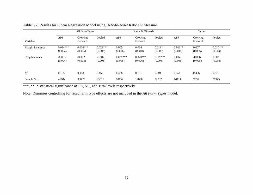
32

Table 5.2: Results for Linear Regression Model using Debt-to-Asset Ratio FR Measure


Variable

APF Growing

Forward

Pooled APF Growing

Forward

Pooled APF Growing

Forward

Pooled

Margin Insurance 0.024***

(0.004)

0.016***

(0.005)

0.022***

(0.003)

0.005

(0.006)

0.014

(0.010)

0.014**

(0.006)

0.011**

(0.006)

0.007

(0.005)

0.010***

(0.004)

Crop Insurance -0.003

(0.004)

-0.002

(0.005)

-0.002

(0.003)

0.029***

(0.005)

0.020***

(0.006)

0.023***

(0.004)

0.004

(0.006)

-0.006

(0.005)

0.002

(0.004)

𝑅2 0.155 0.158 0.153 0.478 0.131 0.204 0.351 0.436 0.376

Sample Size 46884 39067 85951 10152 12080 22232 14114 7831 21945

***, **, * statistical significance at 1%, 5%, and 10% levels respectively

Note: Dummies controlling for fixed farm type effects are not included in the All Farm Types model.

33

the absolute level of FR, an 8.2 percentage point increase in the level of FR given FR is greater

than zero, and a 3 percentage point increase on the probability of an operation having FR at all.

Production insurance enrolment is correlated with an 8.2 percentage point increase in the level of

FR, a 6.3 percentage point increase in the level of FR given FR is greater than zero, and a 2.8

percentage point increase in the probability of a non-zero FR level.

The average absolute level of FR for the sample is 0.496 or about 50 percent, while the

average FR given FR greater than zero is 0.688 or about 70 percent. With an average marginal

effect of margin insurance on the absolute FR level of 10.7 percentage points, margin insurance

enrolment translates to a roughly 20 percent change in FR for the average operation in the sample.

The average marginal effect of margin insurance enrolment is about a 12 percent change in FR for

the average operation with FR greater than zero. Production insurance enrolment translates to

about a 16 percent change in FR for the average operation in the sample and a 9 percent change

for the average operation with FR greater than zero, respectively.

The average marginal effects for the level of FR are higher for the APF policy period

relative to Growing Forward by roughly 8 to 10 percentage points for margin insurance, and about

2 percentage points for production insurance. The average marginal effect on the probability of a

non-zero FR level remains similar across policy periods for both BRM programs.

Average marginal effect estimates are similar for grain and oilseed producers and cattle

operations, but there are several notable distinctions. The average marginal effects of margin

insurance on FR levels are slightly higher for cattle operations than those for the pooled sample

and the grain and oilseed producers by 3 to 7 percentage points. The average marginal effect of

margin insurance on the probability of non-zero FR is larger by almost 3 percentage points for

cattle operations. The larger effect of margin insurance on cattle operations may be in part due to

the lack of alternative BR management tools available to cattle operators relative to other farm

types and the high level of capital inputs necessary for running a cattle operation.

Another notable point is the significant marginal effect of production insurance on FR

levels and probability of non-zero FR. In 2013, Growing Forward 2 introduced new guidelines for

provinces to provide livestock production insurance. Prior to this, production insurance was mainly

designed for crops and horticulture producers. Private price insurance options for livestock exist,

but production insurance is not common. Significant results for production insurance imply cattle

34

producers may supplement their income with crop production or may be producing their feed for

feedlot operations.

5.1.2 Debt-to-Asset Ratio

The estimates from the BRM programs and financial risk analysis using the debt-to-asset

ratio as a measure of FR yield results consistent with the hypothesized relationship but are not as

robust across the different samples. In general, BRM program participation is correlated with a

higher level of FR. Results should be interpreted as percentage point changes to the debt-to-asset

ratio, or FR.

Only margin insurance is significant for the pooled farm type sample. Margin insurance

enrolment is correlated with a 2.4, 1.6, and 2.2 percentage point increase in the level of FR for the

APF, Growing Forward and pooled policy periods, respectively. Results for the farm-specific

samples are distinct and unsurprising. For grain and oilseed producers, production insurance

enrolment is correlated with a 2 to 2.9 percentage point increase in FR across the policy periods,

while margin insurance was not significant except in the pooled policy sample at a 5% significance

level. For cattle operations, margin insurance is correlated with a 1.2 percentage point increase for

the APF period, and 1 percentage point increase for the pooled period sample. Production

insurance does not have a significant effect on the level of FR for cattle producers.

5.1.3 Summary of BRM Programs and Financial Risk Results

The two different theoretical approaches to risk balancing by Gabriel and Baker (1980) and

Collins (1985) yield two different measure of FR and models. Results show that BRM program

participation is correlated with an increase in FR under both FR measures. The main distinction

between the results of the two FR measures is the significance of increased FR associated with

each BRM program. Higher FR is associated with margin insurance and production insurance

participation for the pooled sample, grain and oilseed producers, and cattle operations when using

the fixed debt obligations measure of FR. A greater magnitude in the level of FR associated with

margin insurance is observed for cattle operations. Results from the debt-to-asset measure of FR

vary in the significance of greater FR across samples and insurance types. Results using debt-to-

asset show greater FR is associated with production insurance for grain and oilseed producers and

margin insurance for cattle operations.

35

5.1.4 Discussion

Results show that, across certain policy periods and farm type sample groups, BRM

program participation is correlated with higher levels of FR, but it cannot be said that BRM

programs lead farms to take on greater FR. While a causal relationship cannot be concluded from

the results, the positive correlation between BRM program participation and higher FR provides

policy relevant insights into the sample of BRM program participants. BRM program participants

in the sample have higher levels of FR relative to those that do not participate.

Policymakers should consider the distinct risk profile of participants when designing risk

management programs if higher FR levels are a characteristic of BRM program participants,

regardless of whether higher FR is caused by participation. The Canadian suite of BRM programs

have been created to mitigate and manage BR but not FR. A total risk approach to risk management

programming may be beneficial for the typical farm that would choose to enrol in a BRM program.

5.1.5 Limitations

5.1.5.1 Endogeneity

Endogeneity between BRM program participation and FR levels is an issue that limits

interpretation of the results. Causality between BRM program participation and FR cannot be

drawn because BRM program participation is not exogenously determined. Farms enrolling

themselves in BRM programs causes issues associated with self-selection. The sample of farms

that choose to participate in BRM programs may consist of operations that have higher FR than

those that do not participate. If BRM program participation and higher levels of FR are positively

correlated with an unobserved variable that is not captured in the data, then BRM program

participation would be correlated with higher levels of FR without program participation being the

cause of higher FR.

Previous empirical studies have used panel data to observe whether an increase in FR from

one year to the next is correlated with BRM program participation or payout in the previous year,

but this would not solve the issue of endogeneity due to self-selection (Uzea et al., 2014). Further

research is required to find an instrument for BRM program participation that is exogenous from

FR.

36

Moral hazard cannot be convincingly determined without strong evidence of a causal

relationship between BRM programs and higher levels of FR. If participation in BRM programs

is causing farms to adjust their FR upward, then moral hazard may be present among the sample

of participant, but this cannot be determined through the analysis conducted.

5.1.5.2 Interest Payments over NOI

There are two issues with using the fixed debt obligations or interest payments over NOI

measure of FR. First, interest payments of net-operating-income may not be a good measure of FR

when only observing a cross section. NOI can fluctuate significantly for some farms year to year.

Therefore, an observation of FR from just one year may not accurately represent a farm’s state of

FR. The debt-to-assets measure of FR would likely fluctuate less from year to year for an

individual farm, so the analysis using this measure can be viewed as a robustness test.

Second, results from the tobit model may be biased due to the dropped observations. Farms

with zero and negative values recorded for their net-operating-income are dropped because FR is

measured by dividing fixed financial obligations by net-operating-income. If program

participation is correlated with a higher (lower) FR level or probability of non-zero FR for farms

with zero or negative net-operating-incomes, then the results obtained without these observations

would be biased downward (upward). A bias would imply that farms with zero or negative net-

operating-income values behave differently than operations with positive net-operating-incomes

after controlling for the other variables included in the model. This is plausible as there can be

unobservable characteristics that are correlated an operation's inability to break even, the decision

to participate in BRM programs, and the level of FR. Alternatively, zero and negative values may

only be due to random shocks such as weather and therefore would not affect the estimates. To be

confident in the results, they should be interpreted as reflective of operations only with positive

net-operating-incomes.

5.2 BRM Program Participation and Investment Analysis

BRM program enrollment is correlated with a positive increase in the likelihood of an

investment being made in the same survey period. The level and significance of the average

marginal effects of BRM programs on investment vary between sample periods and types of

operations, but results are generally robust.

37

Tables (5.3) and (5.4) provide estimates for the average marginal effect of production and

margin insurance participation on the likelihood of an investment being made. Estimates are

interpreted as percentage point changes in the probability of the investment outcome. The tables

include the directional effect and significance for the non-binary control variables while the

average marginal effects are not. Table (5.3) displays the average partial effect estimates when

using the FFS binary investment variable. The model is run for grain and oilseed producers, cattle

operations, and a pooled farm type sample across the APF, Growing Forward and pooled policy

periods. Table (5.4) provides a comparison of results under alternative investment variables across

different policy periods using only the pooled farm type sample.

5.2.1 Farm-Type Samples with FFS Investment Variable

The first three columns of Table (5.3) provide the estimates for the pooled farm type sample

across different policy periods. The margin insurance enrolment is correlated with a 4.3, 1.9, and

2.9 percentage point increase in the likelihood of an investment being made for the APF, Growing

Forward, and pooled policy period, respectively. Production insurance enrolment is correlated with

a 3.7, 4.3, and 3.9 percentage point increase in the likelihood of an investment being made for the

same policy period sample groups.

For grain and oilseed producers, average marginal effects for production insurance are

significant, while those for margin insurance are not. Production insurance enrolment is correlated

with a 4.8 percentage point increase in the likelihood of investment for the APF policy period, and

a 3.3 percentage point increase for the pooled policy period. The marginal effect is not significant

for the Growing Forward policy period. These results are consistent with the BRM programs and

FR analysis results using the debt-to-asset measure of FR which found production insurance to be

positive and significant for grain and oilseed producers, while margin insurance was not significant.

For cattle operations, both margin insurance and production insurance enrolment are

correlated with an increased likelihood of investment. Margin insurance is correlated with a 9

percentage point increase for the APF period and a 4.3 percentage point increase in the Growing

Forward period. On the other hand, production insurance enrolment is correlated with a 2.8

percentage point increase for the APF period and a 7.7 percentage point increase in the likelihood

of investment for the Growing Forward period. The magnitude of the average marginal effect for

margin insurance decreased by roughly 5 percentage points between APF and Growing Forward,

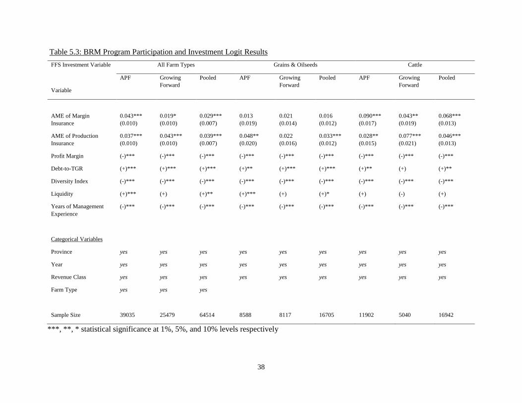
38

Table 5.3: BRM Program Participation and Investment Logit Results

FFS Investment Variable All Farm Types Grains & Oilseeds Cattle

APF Growing

Forward

Pooled APF Growing

Forward

Pooled APF Growing

Forward

Pooled

Variable

AME of Margin

Insurance

0.043***

(0.010)

0.019*

(0.010)

0.029***

(0.007)

0.013

(0.019)

0.021

(0.014)

0.016

(0.012)

0.090***

(0.017)

0.043**

(0.019)

0.068***

(0.013)

AME of Production

Insurance

0.037***

(0.010)

0.043***

(0.010)

0.039***

(0.007)

0.048**

(0.020)

0.022

(0.016)

0.033***

(0.012)

0.028**

(0.015)

0.077***

(0.021)

0.046***

(0.013)

Profit Margin (-)*** (-)*** (-)*** (-)*** (-)*** (-)*** (-)*** (-)*** (-)***

Debt-to-TGR (+)*** (+)*** (+)*** (+)** (+)*** (+)*** (+)** (+) (+)**

Diversity Index (-)*** (-)*** (-)*** (-)*** (-)*** (-)*** (-)*** (-)*** (-)***

Liquidity (+)*** (+) (+)** (+)*** (+) (+)* (+) (-) (+)

Years of Management

Experience

(-)*** (-)*** (-)*** (-)*** (-)*** (-)*** (-)*** (-)*** (-)***

Categorical Variables

Province yes yes yes yes yes yes yes yes yes

Year yes yes yes yes yes yes yes yes yes

Revenue Class yes yes yes yes yes yes yes yes yes

Farm Type yes yes yes

Sample Size 39035 25479 64514 8588 8117 16705 11902 5040 16942


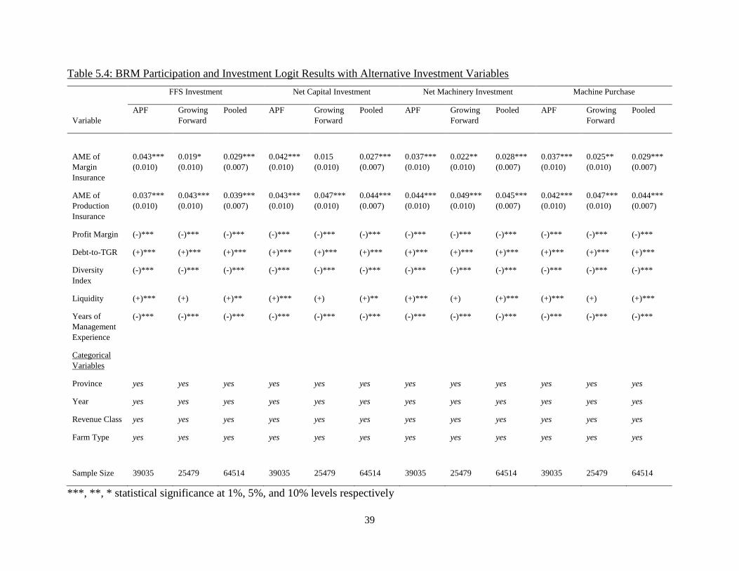
39

Table 5.4: BRM Participation and Investment Logit Results with Alternative Investment Variables

FFS Investment Net Capital Investment Net Machinery Investment Machine Purchase

Variable

APF Growing

Forward

Pooled APF Growing

Forward

Pooled APF Growing

Forward

Pooled APF Growing

Forward

Pooled

AME of

Margin

Insurance

0.043***

(0.010)

0.019*

(0.010)

0.029***

(0.007)

0.042***

(0.010)

0.015

(0.010)

0.027***

(0.007)

0.037***

(0.010)

0.022**

(0.010)

0.028***

(0.007)

0.037***

(0.010)

0.025**

(0.010)

0.029***

(0.007)

AME of

Production

Insurance

0.037***

(0.010)

0.043***

(0.010)

0.039***

(0.007)

0.043***

(0.010)

0.047***

(0.010)

0.044***

(0.007)

0.044***

(0.010)

0.049***

(0.010)

0.045***

(0.007)

0.042***

(0.010)

0.047***

(0.010)

0.044***

(0.007)

Profit Margin (-)*** (-)*** (-)*** (-)*** (-)*** (-)*** (-)*** (-)*** (-)*** (-)*** (-)*** (-)***

Debt-to-TGR (+)*** (+)*** (+)*** (+)*** (+)*** (+)*** (+)*** (+)*** (+)*** (+)*** (+)*** (+)***

Diversity

Index

(-)*** (-)*** (-)*** (-)*** (-)*** (-)*** (-)*** (-)*** (-)*** (-)*** (-)*** (-)***

Liquidity (+)*** (+) (+)** (+)*** (+) (+)** (+)*** (+) (+)*** (+)*** (+) (+)***

Years of

Management

Experience

(-)*** (-)*** (-)*** (-)*** (-)*** (-)*** (-)*** (-)*** (-)*** (-)*** (-)*** (-)***

Categorical

Variables

Province yes yes yes yes yes yes yes yes yes yes yes yes

Year yes yes yes yes yes yes yes yes yes yes yes yes

Revenue Class yes yes yes yes yes yes yes yes yes yes yes yes

Farm Type yes yes yes yes yes yes yes yes yes yes yes yes

Sample Size 39035 25479 64514 39035 25479 64514 39035 25479 64514 39035 25479 64514


40

while the average marginal effect for production insurance increased by about 5 percentage points

between the two policy periods. The increase in the marginal effect of production insurance may

be in part due to adjustments made to AgriInsurance following Growing Forward 2 which tailored

the program for livestock, thus increasing its effect on BR. Alternatively, production insurance

may have become more relevant to cattle operations' business decisions if the income share

affected by production insurance increased. As production insurance is commonly designed for

crops, a greater share of income arising from crop production may lead to a greater influence of

production insurance on investment behaviour.

The rows below the average marginal effects for the BRM programs provide the sign and

significance of the coefficients for each non-categorical covariate, while the average marginal

effects are not calculated.1 The sign and significance still provide interesting insights into factors

correlated with the decision to invest. Results show that a farm's net operating income over total

gross revenue is significant and negatively correlated with the likelihood of an investment being

made, contrary to what was hypothesized. Higher profit margin measures may be correlated with

higher efficiency farms which are less likely to invest. Debt-to-total gross revenue is significant

and positively correlated with the likelihood of investment. The positive correlation is also

contrary to the hypothesized effect, as the expected sign was negative. There is a simultaneity issue

with this variable since investment can increase debt-to-total gross revenue when both are only

observed in the same narrow time frame. Diversification is significant and negatively correlated

with the likelihood of investment, while the expected sign of the diversity index coefficient was

expected to be positive. In general, studies examining farm diversification find that farms with

greater diversity tend to be smaller and less wealthy (Pope and Prescott, 1980; Mishra et al., 2004;

Melhim et al., 2009). The theory that farms give up on gains from economies of scale in favour of

risk reduction through diversity is used to explain this observation. Farms with higher

diversification may be less likely to invest in capital to grow their operations. Liquidity is

positively correlated with the likelihood of investment but is not significant across all sample

groups. Liquidity is significant for the pooled farm type sample across the APF and pooled policy

period. It is also significant for the APF policy period, and pooled policy period at the 10%

1Average marginal effects were not calculated due to limited time with the data and limited

capability of the hardware used for the analysis.

41

significance level, for grain and oilseed producers. The positive correlation is consistent with the

hypothesized sign. Liquidity is not significant for cattle operations. This may be due to how

working capital is calculated for the liquidity measure. The current assets and current debts used

to calculate working capital are not as relevant to livestock operations as they are to crop

production. Year of management experience is significant and negatively correlated with

investment, as expected. Of the categorical fixed effect variables, the coefficients for revenue class

were consistently significant and worth noting. As revenue increases by each category, the

magnitude of the effect on the likelihood of investment increases relative to the lowest revenue

category.

5.2.2 Alternative Capital Investment Variables

Results using the alternative investment variables are consistent with the results obtained

using the FFS investment variable. The magnitude of the average partial effects differs slightly

from results using the FFS investment variable. The significance and sign of the other non-

categorical variables are robust across investment variables.

While most of the results do not change, the significance of margin insurance enrolment

on investment behaviour over the Growing Forward policy period varies across investment

variables. Margin insurance enrolment for the Growing Forward period is correlated with a 1.9

percentage point increase in the likelihood of investment using the FFS investment variable and is

only significant at the 10 percent significance level. The average marginal effect for margin

insurance is not significant over the Growing Forward period for the net capital investment

variable, but it is significant at the 5 percent significance level using the net machinery investment

variable and the machine purchase variable. Margin insurance is correlated with a 2.2 percentage

point increase in the likelihood of net machinery investment being positive and a 2.5 percentage

point increase in the likelihood of an operation purchasing machinery. The way machinery

investments were financed during the Growing Forward period may explain the greater

significance of margin insurance on machinery related investment variables relative to less specific

investment variables. If machinery investments are commonly financed through debt, more so than

other forms of capital, then machinery investments are more directly linked to FR, and therefore

the FR and BRM program enrolment relationship analyzed above.

42

Production insurance generally has a larger average marginal effect than margin insurance

across the four capital investment variables. These results may reflect how production insurance

and margin insurance, specifically AgriStability during the Growing Forward period, are designed

to interact. When calculating an operation’s margin to determine if they are to receive an indemnity

from margin insurance, payouts from production insurance are included as revenue. This means

that a payout from production insurance reduces the likelihood of a payout from margin insurance.

The lower likelihood of a payout from margin insurance when an operation is also enrolled in

production insurance may reduce the effect of margin insurance on investment behaviour.

5.2.3 Discussion

5.2.3.1 Causal Relationship between BRM Program Participation and Investment

It is difficult to isolate the effect of BRM programs on FR and investment due to the self-

selection of BRM program participants and the timing of participation and investment decisions.

The risk balancing theory states that in the event of an exogenous shock to a component of total

risk, a different component will adjust to maintain the accepted level of total risk (Gabriel and

Baker, 1980). Neither BRM program participation or capital investment can be considered as

exogenous shocks to a firm's total risk portfolio. The risk balancing framework can provide insight

into how BR and FR adjust due to program participation and investment decisions, but a causal

relationship between the variables is difficult to draw without exogenous shocks that effect BRM

program participation or investment. The analysis conducted in this paper cannot show that a

reduction in BR due to program participation caused FR though investment to increase. Likewise,

it cannot show that an increase in FR due to investment caused BR to decrease due to subsequent

program participation.

The timing of BRM program participation and investment decision makes it difficult to

isolate a causal effect of BRM program participation on investment behaviour and vice versa. The

data is in the form of repeated cross-sections with a new sample selected each survey year. We can

see whether an operation enrolled in a BRM program and made an investment sometime within

the survey reference year, but we cannot tell when within this period each decision was made. The

deadline for enrolling in margin insurance and production insurance is generally in April or early

May. Investment can happen before or after enrolment within the survey reference year. That said,

panel data or other data where the specific timing of investment and BRM program participation

43

is known may not solve the problem. The decision to invest or participate is not necessarily made

at the time investment, or enrollment occurs.

As stated above, neither investment or BRM program enrolment are exogenously

determined for a farm. The decision to participate in a BRM program and the decision to invest

may be a joint decision, even if one decision is executed before the other. For example, an

operation intending on making a large investment may take steps to ensure a level of income to

finance the resulting debt and enrol in a BRM program. Similarly, knowing that BRM programs

are available, an operation may be encouraged to invest. With panel data, the order of BRM

program enrolment and investment occurring could be known but would not necessarily prove a

causal relationship.

5.2.3.2 BRM Programs Help Farms that Invest

The policy-relevant interpretation of the results is that BRM programs help farms that want

to invest. A multitude of factors in agriculture determine investment behaviour, and while there is

evidence that income volatility, or BR, is a factor in the likelihood and level of capital investment

made by farms, it is unlikely to be the driving factor for investment. BRM programs are designed

to reduce income volatility which can facilitate investment through mechanisms discussed above

such as credit availability and the ability to finance debt. Farms that want to invest may enrol in

BRM programs while BRM programs may provide the opportunity for a farm to invest. This

interpretation does not speak to causality which is consistent with the empirical analysis. The

positive correlation between BRM program participation and investment indicates that farm

operators who are enrolled in BRM programs are more likely to invest without implying a causal

relationship. In this context, BRM programs do more than fulfil their short-term purpose of

managing business risk. BRM programs are tools that can be used when making business decisions

such as investment. BRM programs can have policy implications regarding growth and innovation

within the agricultural industry.

5.2.3.3 Perceived Business Risk Reduction through BRM Programs

While this paper does not directly address risk balancing behaviour in the empirical

analysis, it is worth discussing risk balancing within the BRM program and investment relationship.

Under a risk balancing framework, BRM program participation can be viewed as a reduction in an

44

operation’s BR, relative to not participating. The assumption that BRM programs reduce BR is

needed. A weaker alternative assumption is proposed in which BRM program participation causes

a perceived BR reduction. This weaker assumption may be sufficient to establish risk balancing if

risk balancing is a behaviour that is not strongly rooted in financial figures. Risk balancing without

financial analysis is an unreasonable assumption for most businesses but may be valid in the case

of agricultural operations as there is evidence of poor business planning and record keeping among

Canadian farms (Serecon Management Consulting Inc., 2009). If higher FR is correlated with

perceived BR reductions, this may have negative implications for the overall financial health of

farms. Previous studies highlight the issue of risk balancing and BRM program participation,

finding that BRM programs may reduce the use of other risk-mitigating tools and can increase the

likelihood of default (Featherstone et al., 1988; Fernandez-Villaverde et al., 2011; Uzea et al.,

2014; Vercammen, 2007). This paper takes the view that benefits from risk balancing can arise

through investment, but if BRM program participation does not reduce BR, the potential benefits

from an investment may be outweighed by the increase in total risk due to increased FR without

the offsetting reduction in BR.

5.2.4 Limitations

5.2.4.1 Observed Variables and Correlation

As the data is repeated cross-sections, BRM program enrolment and investment occurring

outside of the survey year for a specific farm operation will not be observed. Therefore, the

correlation between BRM program enrolment and investment is only observed when both occur

within the same survey year. This is a shortcoming of the analysis as the relationship between the

two decisions would not be restricted by this survey reference period. Panel data may help solve

this problem by expanding the period in which BRM program participation and investment can be

observed, but the determining a limit to this period would require further research.

5.2.4.2 Endogeneity

Two endogeneity issues may present in the analysis. One is due to omitted variables and

the other due to simultaneity. Endogeneity may cause biased estimates of the relationship between

BRM program enrollment and investment.

45

The models used in the analysis may omit unobservable characteristics of some operations

that are correlated with the decision to enrol in a BRM program and the decision to invest. For

example, operations with better-established business plans or those that use professional

accounting firms may be more focused on growing their farm business and are therefore more

likely to make investments. Such operations may also have better information on BRM programs

and would be more likely to participate. Another source of endogeneity may arise from a period

of high income for an operation prior to the observable survey year. Periods of high income may

encourage a farm to enrol in margin insurance since their coverage is based on historical margins.

High income periods may also increase the likelihood of investment due to increased availability

of capital. BRM program enrolment and investment behaviour would be positively correlated to

high income periods preceding the observable survey year and, therefore, to each other. These

potential sources of endogeneity cause BRM program participation and investment to be correlated

with the error term in the latent model for the logit, meaning the assumed logistic distribution of

this error term is incorrect. The missing variable bias arises from self-selection of BRM program

participants.

BRM program enrolment and investment may be a joint decision, as discussed above, and

would cause a simultaneity issue. Estimating a model with investment as the dependent variable

and BRM program enrolment as the independent variable will cause BRM program enrolment to

be correlated with the error term, possibly biasing the results.

5.3 Evaluating Results with respect to Policy Goals

As BRM programs are a policy tool, the question arises of whether the results of this paper

align with the stated policy goals. This paper does not investigate the primary goal of reduced

income volatility, but it does address two specific general principles of risk management

programming stated in the framework agreement for Growing Forward. The first general principle

stated that “programs should minimize moral hazard” (Agriculture and Agri-Food Canada, 2008).

Moral hazard refers to the change in behaviour when faced with a reduction in risk. This paper

finds that BRM program participation is correlated with higher levels of FR and an increase in the

likelihood of an investment being made. Moral hazard cannot definitively be said to exist without

establishing a causal relationship between BRM program participation and higher levels of FR or

investment behaviour.

46

The second general principle stated that “programs should contribute to market-oriented

adjustments and adoption of technological innovations” (Agriculture and Agri-Food Canada,

2008). Although we cannot tell if the capital investments in our sample are in technological

innovations, it is feasible that some are, especially machine investments. In the context of larger

agricultural policy initiatives of innovation and growth, the positive correlation between BRM

program enrolment and investment behaviour provides evidence that BRM programs are aligned

with such policy goals.

Further analysis may be done to determine whether an investment is financed through debt,

therefore effecting an operation’s level of FR. Analysis of productivity gains due to investments

financed through debt may provide better evidence of the long-term benefits of BRM programs

such as increased productivity and efficiency. Possible capitalization of these productivity gains

could be addressed as well.

47

6 CONCLUSION

Studies have shown that Canadian BRM programs are likely fulfilling their primary role

of reducing BR faced by agricultural producers (Agriculture and Agri-Food Canada, 2012; Uzea

et al., 2014). Through risk balancing behaviour, reductions in BR through BRM program

enrolment may be correlated with other risk influencing farm behaviour. While previous studies

frame BRM programs and risk balancing as having neutral or even negative consequences

regarding farm behaviour and risk, this paper finds BRM program enrolment to be correlated with

increased likelihood of investment. The positive relationship between BRM program enrolment

and investment has implication for farm’s productivity, long-term financial health, and growth.

A causal effect cannot be drawn between BRM program enrolment and investment

behaviour based on the analysis. BRM programs are self-enrolled programs that can be factored

into many farm-level decisions, with enrollment as a farm-level decision itself. BRM program

enrolment is very likely an endogenous decision, so a unidirectional causal effect on investment

would not be a policy-relevant measure as it does not capture the entire relationship between the

two variables. While we cannot say how one directly affects the other, the positive correlation

between BRM program enrolment and investment behaviour highlights that policies targeted at

one aspect of the agricultural industry may be indirectly related to others. In the case of agricultural

BRM programs, policymakers should keep in mind the linkages between factors that influence

risk, as well as farm-level decisions that are influenced by risk.

Despite data limitations and shortcomings of the analysis, this paper provides evidence of

a positive relationship between BRM program enrolment and investment behaviour. The indirect

effects of adjusting risk on farm-level behaviour and decision-making are important to consider

when designing policy and evaluating existing programs. It is also important to consider the

context in which farm decisions are viewed as the relationship between BRM program enrolment

and investment can be viewed as an example of moral hazard or farms optimizing their business

through risk management tools.

48

REFERENCES

Agriculture and Agri-Food Canada. (2005). Agriculture Policy Framework: Federal-provincial-

territorial programs / prepared by Program Planning, Integration and Management

Directorate. Retrieved from http://publications.gc.ca/site/eng/268229/publication.html

Agriculture and Agri_Food Canada. (2008). Growing Forward: A federal - provincial -

territorial framework agreement on agriculture, agri-food and agri-based products policy.

Retrieved from http://www.publications.gc.ca/site/eng/370293/publication.html

Agriculture and Agri-Food Canada. (2012). Evaluation of income stability tools - AgriStability

and AgriInvest report. Retrieved from http://www.agr.gc.ca/eng/about-us/offices-and-

locations/office-of-audit-and-evaluation/evaluation-reports/evaluation-of-income-stability-

tools-agristability-and-agriinvest/?id=1362083604412

Agriculture and Agri-Food Canada. (2018). AgriInvest. Retrieved from

http://www.agr.gc.ca/eng/?id=1291828779399#l1

Babcock, B. A., & Hennessy, D. A. (1996). Input demand under yield and revenue insurance.

American Journal of Agricultural Economics, 78(2), 416.

Baum, C., Caglayan, M., & Talavera, O. (2010). On the sensitivity of firms' investment to cash

flow and uncertainty. Oxford Economic Papers, 62(2), 286-306.

Benjamin, C., & Phimister, E. (2002). Does capital market structure affect farm investment? A

comparison using french and british farm-level panel data. American Journal of

Agricultural Economics, 84(4), 1115-1129.

Bierlen, R., & Featherstone, A. (1998). Fundamental q, cash flow, and investment: Evidence

from farm panel data. The Review of Economics and Statistics, 80(3), 427-435.

Bloom, N., Bond, S., & Van Reenen, J. (2007). Uncertainty and investment dynamics. Review of

Economic Studies, 74(2), 391-415.

Boyle, G., & Guthrie, G. (2003). Investment, uncertainty, and liquidity. Journal of Finance,

58(5), 2143-2166.

Caballero, R., & Pindyck, R. (1996). Uncertainty, investment, and industry evolution.

International Economic Review, 37(3), 641-662.

Coble, K., Heifner, R., & Zuniga, M. (2000). Implications of crop yield and revenue insurance

for producer hedging. Journal of Agricultural and Resource Economics, 25(2), 432-452.

Chaddad, F., Cook, M., & Heckelei, T. (2005). Testing for the presence of financial constraints

in us agricultural cooperatives: An investment behaviour approach. Journal of Agricultural

Economics, 56(3), 385-397.

Collins, R. (1985). Expected utility, debt-equity structure, and risk balancing. American Journal

of Agricultural Economics, 67(3), 627-629.

49

De Mey, Y., Van Winsen, F., Wauters, E., Vancauteren, M., Lauwers, L., & Van Passel, S.

(2014). Farm-level evidence on risk balancing behavior in the eu-15. Agricultural Finance

Review, 74(1), 17-37.

Doshi, H., Kumar, P., Yerramilli, V. (2017) Uncertainty, capital investment, and risk

management. Management Science.

Escalante, C., & Barry, P. (2003). Determinants of the strength of strategic adjustments in farm

capital structure. Journal of Agricultural and Applied Economics, 35(01), 67-78.

Featherstone, A., Moss, C., Baker, T., & Preckel, P. (1988). The theoretical effects of farm

policies on optimal leverage and the probability of equity losses. American Journal of


Fernandez-Villaverde, J., Guerron-Quintana, P., Rubio-Ramirez, J. F., & Uribe, M. (2011). Risk

matters: The real effects of volatility shocks. American Economic Review, 101(6), 2530-

2561.

Gabriel, S., & Baker, C. (1980). Concepts of business and financial risk. American Journal of


Ghosal, V., & Loungani, P. (2000). The differential impact of uncertainty on investment in small

and large businesses. Review of Economics and Statistics, 82(2), 338-343.

Greene, W. (2012). Econometric analysis (7th ed.). Boston: Prentice Hall.

Heikkinen, T., & Pietola, K. (2009). Investment and the dynamic cost of income uncertainty: The

case of diminishing expectations in agriculture. European Journal of Operational

Research, 192(2), 634-646.

Hennessy, D. (1998). The production effects of agricultural income support policies under

uncertainty. American Journal of Agricultural Economics, 80(1), 46-57.

Hughes, W., Penson, J., & Bednarz, C. (1984). Subsidized credit and investment in agriculture:

the special case of farm real estate. American Journal of Agricultural Economics, 66(5),

755-760.

Ifft, J., Kuethe, T., & Morehart, M. (2015). Does federal crop insurance lead to higher farm debt

use? Evidence from the Agricultural Resource Management Survey (ARMS). Agricultural

Finance Review, 75(3), 349-367.

Kallas, Z., Serra, T., & Gil, J. (2012). Effects of policy instruments on farm investments and

production decisions in the Spanish COP sector. Applied Economics, 44(30), 3877-3886.

Melhim, A., O'Donoghue, E., & Shumway, C. (2009). What does initial farm size imply about

growth and diversification? Journal of Agricultural and Applied Economics, 41(1), 193-

206.

Minton, B. A. & Schrand. C. (1999). The impact of cash flow volatility on discretionary

investment and the costs of debt and equity financing. Journal of Financial Economics,

54(3), 423-460.

50

Mishra, A., El-Osta, H., & Sandretto, C. (2004). Factors affecting farm enterprise diversification.

Agricultural Finance Review, 64(2), 151-166.

O'Donoghue, E., & Whitaker, J. (2010). Do direct payments distort producers' decisions? An

examination of the Farm Security and Rural Investment Act of 2002. Applied Economic

Perspectives and Policy, 32(1), 170-193.

O'Toole, C., Newman, C., & Hennessy, T. (2014). financing constraints and agricultural

investment: Effects of the Irish financial crisis. Journal of Agricultural Economics, 65(1),

152-176.

Pope, R., & Prescott, R. (1980). Diversification in relation to farm size and other socioeconomic

characteristics. American Journal of Agricultural Economics, 62(3), 554-559.

Ramaswami, B. (1993). Supply response to agricultural insurance: Risk reduction and moral

hazard effects. American Journal of Agricultural Economics, 75(4), 914-925.

Saskatchewan Crop Insurance Corporation (2018) Guide to understanding crop insurance.

Available from https://www.saskcropinsurance.com/ci/multi-peril/

Sckokai, P., & Moro, D. (2009). Modelling the impact of the CAP Single Farm Payment on farm

investment and output. European Review of Agricultural Economics, 36(3), 395-423.

Serecon Management Consulting Inc. (2009). Agricultural risk management survey report for

Policy, Strategy and Intergovernmental Affairs Division.

Smith, V., & Goodwin, B. (1996). Crop insurance, moral hazard, and agricultural chemical use.

American Journal of Agricultural Economics, 78(2), 428-438.

Statistics Canada. (2018). Farms Classified by Farm Type, Historical Data. Table: 32-10-0166-

01. Available from https://www150.statcan.gc.ca/t1/tbl1/en/tv.action?pid=3210016601

Statistics Canada. (2018). Farms Classified by Size, Historical Data. Table: 32-10-0156-01.

Available from https://www150.statcan.gc.ca/t1/tbl1/en/tv.action?pid=3210015601

Statistics Canada. (2018). Farms Classified by Total Gross Farm Receipts, 2015 Constant

Dollars, Historical Data. Table: 32-10-0157. Available from

https://www150.statcan.gc.ca/t1/tbl1/en/tv.action?pid=3210015701

Turvey, C. (2012). Whole farm income insurance. The Journal of Risk and Insurance, 79(2),

515-540.

Uzea, N., Poon, K., Sparling, D., & Weersink, A. (2014). Farm support payments and risk

balancing: Implications for financial riskiness of Canadian farms. Canadian Journal of

Agricultural Economics/Revue Canadienne D'agroeconomie, 62(4), 595-618.

Vercammen, J. (2007). Farm bankruptcy risk as a link between direct payments and agricultural

investment. European Review of Agricultural Economics, 34(4), 479-500.

Wooldridge, J. (2010). Econometric analysis of cross section and panel data (Vol. 8). The MIT

Press.

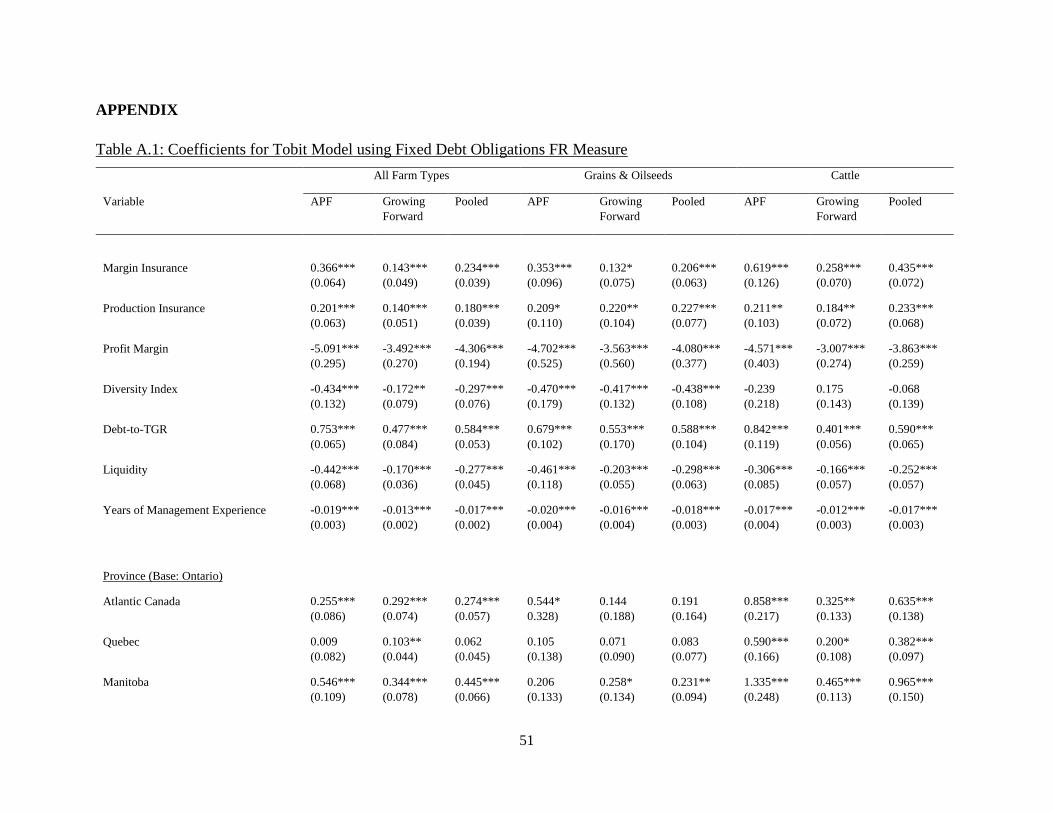
51

APPENDIX

Table A.1: Coefficients for Tobit Model using Fixed Debt Obligations FR Measure


Variable APF Growing

Forward

Pooled APF Growing

Forward

Pooled APF Growing

Forward

Pooled


(0.064)

0.143***

(0.049)

0.234***

(0.039)

0.353***

(0.096)

0.132*

(0.075)

0.206***

(0.063)

0.619***

(0.126)

0.258***

(0.070)

0.435***

(0.072)

Production Insurance 0.201***

(0.063)

0.140***

(0.051)

0.180***

(0.039)

0.209*

(0.110)

0.220**

(0.104)

0.227***

(0.077)

0.211**

(0.103)

0.184**

(0.072)

0.233***

(0.068)

Profit Margin -5.091***

(0.295)

-3.492***

(0.270)

-4.306***

(0.194)

-4.702***

(0.525)

-3.563***

(0.560)

-4.080***

(0.377)

-4.571***

(0.403)

-3.007***

(0.274)

-3.863***

(0.259)

Diversity Index -0.434***

(0.132)

-0.172**

(0.079)

-0.297***

(0.076)

-0.470***

(0.179)

-0.417***

(0.132)

-0.438***

(0.108)

-0.239

(0.218)

0.175

(0.143)

-0.068

(0.139)

Debt-to-TGR 0.753***

(0.065)

0.477***

(0.084)

0.584***

(0.053)

0.679***

(0.102)

0.553***

(0.170)

0.588***

(0.104)

0.842***

(0.119)

0.401***

(0.056)

0.590***

(0.065)

Liquidity -0.442***

(0.068)

-0.170***

(0.036)

-0.277***

(0.045)

-0.461***

(0.118)

-0.203***

(0.055)

-0.298***

(0.063)

-0.306***

(0.085)

-0.166***

(0.057)

-0.252***

(0.057)

Years of Management Experience -0.019***

(0.003)

-0.013***

(0.002)

-0.017***

(0.002)

-0.020***

(0.004)

-0.016***

(0.004)

-0.018***

(0.003)

-0.017***

(0.004)

-0.012***

(0.003)

-0.017***

(0.003)

Province (Base: Ontario)

Atlantic Canada 0.255***

(0.086)

0.292***

(0.074)

0.274***

(0.057)

0.544*

0.328)

0.144

(0.188)

0.191

(0.164)

0.858***

(0.217)

0.325**

(0.133)

0.635***

(0.138)

Quebec 0.009

(0.082)

0.103**

(0.044)

0.062

(0.045)

0.105

(0.138)

0.071

(0.090)

0.083

(0.077)

0.590***

(0.166)

0.200*

(0.108)

0.382***

(0.097)

Manitoba 0.546***

(0.109)

0.344***

(0.078)

0.445***

(0.066)

0.206

(0.133)

0.258*

(0.134)

0.231**

(0.094)

1.335***

(0.248)

0.465***

(0.113)

0.965***

(0.150)

52

Saskatchewan 0.677***

(0.121)

0.436***

(0.086)

0.559***

(0.073)

0.446***

(0.169)

0.462***

(0.175)

0.465***

(0.122)

1.302***

(0.206)

0.487***

(0.104)

0.918***

(0.122)

Alberta 0.260***

(0.081)

0.248**

(0.105)

0.249***

(0.065)

0.124

(0.110)

0.314

(0.198)

0.234*

(0.122)

0.754***

(0.159)

0.217**

(0.094)

0.502***

(0.095)

British Columbia -0.062

(0.122)

0.034

(0.095)

-0.028

(0.074)

0.423

(0.257)

0.065

(0.277)

0.215

(0.195)

0.437**

(0.186)

0.007

(0.197)

0.185

(0.137)

Revenue Class (Base: $25,000 to

$99,999)

$100,000 to $249,999 0.960***

(0.166)

0.644***

(0.079)

0.837***

(0.079)

0.850***

(0.156)

0.656***

(0.134)

0.757***

(0.103)

0.691***

(0.126)

0.544***

(0.117)

0.677***

(0.096)

$250,000 to $999,999 1.320***

(0.162)

0.897***

(0.118)

1.177***

(0.113)

1.179***

(0.251)

1.094***

(0.242)

1.160***

(0.170)

1.138***

(0.244)

0.520***

(0.101)

0.893***

(0.152)

$1,000,000 and over 1.593***

(0.220)

1.001***

(0.145)

1.357***

(0.140)

1.253***

(0.227)

1.195***

(0.300)

1.274***

(0.188)

2.057***

(0.575)

0.654***

(0.128)

1.348***

(0.282)

Farm Type (Base: Grains & Oilseeds)

Horticulture 0.045

(0.091)

-0.077

(0.051)

-0.044

(0.050)

Dairy 0.335***

(0.106)

0.056

(0.044)

0.185***

(0.054)

Cattle 0.405***

(0.078)

0.231***

(0.049)

0.329***

(0.046)

Hog 0.190*

(0.113)

0.275***

(0.095)

0.221***

(0.074)

Poultry 0.119

(0.156)

0.016

(0.069)

0.038

(0.081)

Year (Base: changes between samples)

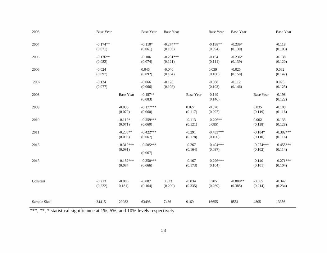
53

2003 Base Year

s

Base Year Base Year Base Year Base Year Base Year

2004 -0.174**

(0.071)

-0.110*

(0.061)

-0.274***

(0.106)

-0.198**

(0.094)

-0.239*

(0.130)

-0.118

(0.103)

2005 -0.176**

(0.082)

-0.106

(0.074)

-0.251***

(0.121)

-0.154

(0.111)

-0.236*

(0.139)

-0.138

(0.120)

2006 -0.024

(0.097)

0.045

(0.092)

-0.040

(0.164)

0.039

(0.180)

-0.025

(0.158)

0.082

(0.147)

2007 -0.124

(0.077)

-0.066

(0.066)

-0.128

(0.108)

-0.088

(0.103)

-0.112

(0.146)

0.025

(0.125)

2008 Base Year -0.187**

(0.083)

Base Year -0.149

(0.146)

Base Year -0.198

(0.122)

2009 -0.036

(0.072)

-0.177***

(0.060)

0.027

(0.117)

-0.078

(0.092)

0.035

(0.119)

-0.109

(0.116)

2010 -0.119*

(0.071)

-0.259***

(0.060)

-0.113

(0.121)

-0.206**

0.085)

0.002

(0.128)

-0.133

(0.128)

2011 -0.233**

(0.093)

-0.422***

(0.067)

-0.291

(0.178)

-0.433***

(0.100)

-0.184*

(0.110)

-0.382***

(0.116)

2013 -0.312***

(0.091)

-0.505***

(0.067)

-0.267

(0.164)

-0.404***

(0.097)

-0.274***

(0.102)

-0.455***

(0.114)

2015 -0.182***

(0.084

-0.350***

(0.066)

-0.167

(0.173)

-0.296***

(0.104)

-0.140

(0.101)

-0.271***

(0.104)

Constant -0.213

(0.222)

-0.086

0.181)

-0.087

(0.164)

0.333

(0.299)

-0.034

(0.335)

0.205

(0.269)

-0.809**

(0.385)

-0.065

(0.214)

-0.342

(0.234)

Sample Size 34415 29083 63498 7486 9169 16655 8551 4805 13356


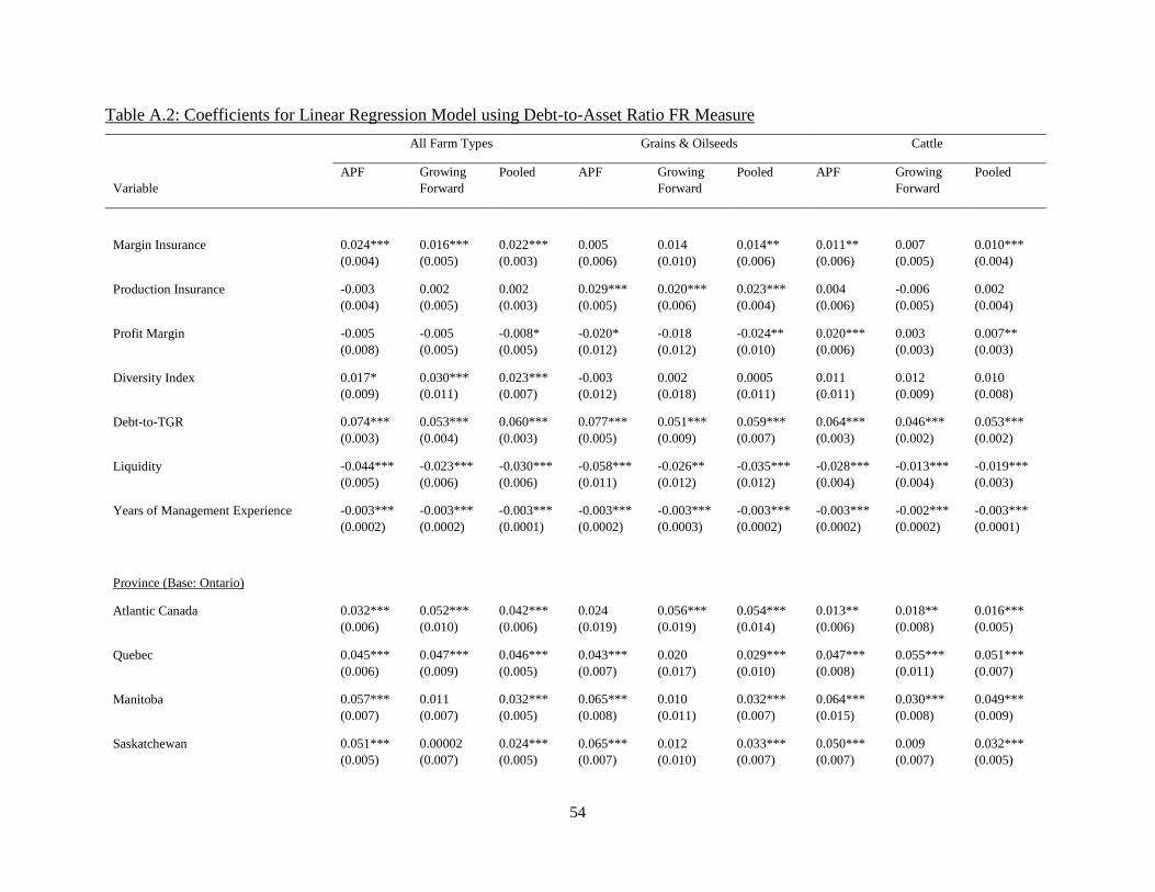
54

Table A.2: Coefficients for Linear Regression Model using Debt-to-Asset Ratio FR Measure


Variable

APF Growing

Forward

Pooled APF Growing

Forward

Pooled APF Growing

Forward

Pooled


(0.004)

0.016***

(0.005)

0.022***

(0.003)

0.005

(0.006)

0.014

(0.010)

0.014**

(0.006)

0.011**

(0.006)

0.007

(0.005)

0.010***

(0.004)

Production Insurance -0.003

(0.004)

0.002

(0.005)

0.002

(0.003)

0.029***

(0.005)

0.020***

(0.006)

0.023***

(0.004)

0.004

(0.006)

-0.006

(0.005)

0.002

(0.004)

Profit Margin -0.005

(0.008)

-0.005

(0.005)

-0.008*

(0.005)

-0.020*

(0.012)

-0.018

(0.012)

-0.024**

(0.010)

0.020***

(0.006)

0.003

(0.003)

0.007**

(0.003)

Diversity Index 0.017*

(0.009)

0.030***

(0.011)

0.023***

(0.007)

-0.003

(0.012)

0.002

(0.018)

0.0005

(0.011)

0.011

(0.011)

0.012

(0.009)

0.010

(0.008)

Debt-to-TGR 0.074***

(0.003)

0.053***

(0.004)

0.060***

(0.003)

0.077***

(0.005)

0.051***

(0.009)

0.059***

(0.007)

0.064***

(0.003)

0.046***

(0.002)

0.053***

(0.002)

Liquidity -0.044***

(0.005)

-0.023***

(0.006)

-0.030***

(0.006)

-0.058***

(0.011)

-0.026**

(0.012)

-0.035***

(0.012)

-0.028***

(0.004)

-0.013***

(0.004)

-0.019***

(0.003)


(0.0002)

-0.003***

(0.0002)

-0.003***

(0.0001)

-0.003***

(0.0002)

-0.003***

(0.0003)

-0.003***

(0.0002)

-0.003***

(0.0002)

-0.002***

(0.0002)

-0.003***

(0.0001)



(0.006)

0.052***

(0.010)

0.042***

(0.006)

0.024

(0.019)

0.056***

(0.019)

0.054***

(0.014)

0.013**

(0.006)

0.018**

(0.008)

0.016***

(0.005)

Quebec 0.045***

(0.006)

0.047***

(0.009)

0.046***

(0.005)

0.043***

(0.007)

0.020

(0.017)

0.029***

(0.010)

0.047***

(0.008)

0.055***

(0.011)

0.051***

(0.007)

Manitoba 0.057***

(0.007)

0.011

(0.007)

0.032***

(0.005)

0.065***

(0.008)

0.010

(0.011)

0.032***

(0.007)

0.064***

(0.015)

0.030***

(0.008)

0.049***

(0.009)

Saskatchewan 0.051***

(0.005)

0.00002

(0.007)

0.024***

(0.005)

0.065***

(0.007)

0.012

(0.010)

0.033***

(0.007)

0.050***

(0.007)

0.009

(0.007)

0.032***

(0.005)

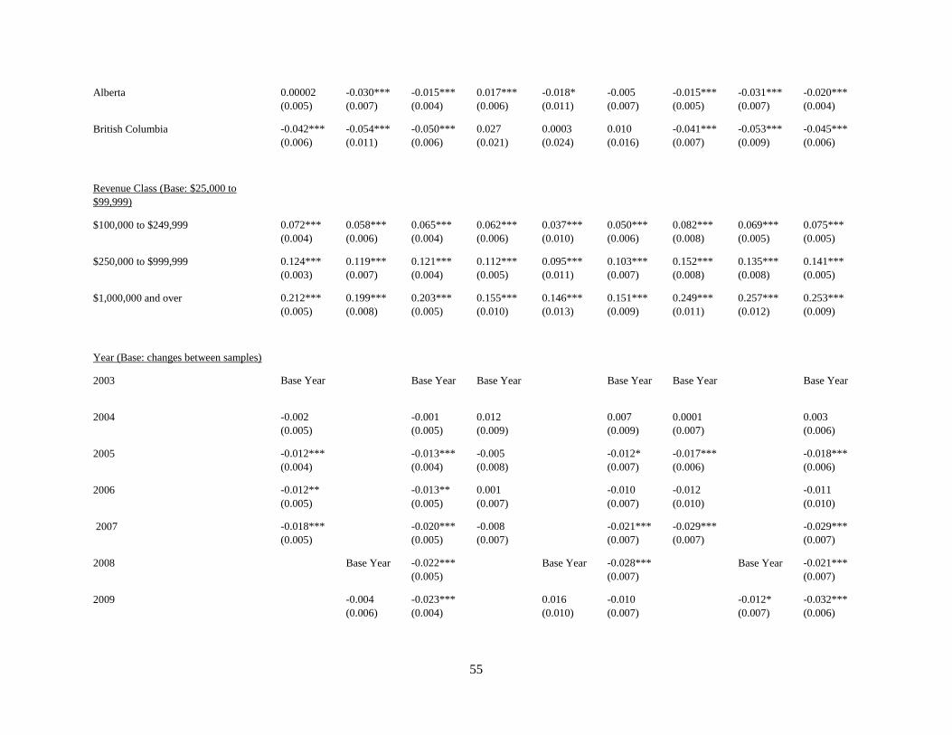
55

Alberta 0.00002

(0.005)

-0.030***

(0.007)

-0.015***

(0.004)

0.017***

(0.006)

-0.018*

(0.011)

-0.005

(0.007)

-0.015***

(0.005)

-0.031***

(0.007)

-0.020***

(0.004)

British Columbia -0.042***

(0.006)

-0.054***

(0.011)

-0.050***

(0.006)

0.027

(0.021)

0.0003

(0.024)

0.010

(0.016)

-0.041***

(0.007)

-0.053***

(0.009)

-0.045***

(0.006)


$99,999)

$100,000 to $249,999 0.072***

(0.004)

0.058***

(0.006)

0.065***

(0.004)

0.062***

(0.006)

0.037***

(0.010)

0.050***

(0.006)

0.082***

(0.008)

0.069***

(0.005)

0.075***

(0.005)

$250,000 to $999,999 0.124***

(0.003)

0.119***

(0.007)

0.121***

(0.004)

0.112***

(0.005)

0.095***

(0.011)

0.103***

(0.007)

0.152***

(0.008)

0.135***

(0.008)

0.141***

(0.005)

$1,000,000 and over 0.212***

(0.005)

0.199***

(0.008)

0.203***

(0.005)

0.155***

(0.010)

0.146***

(0.013)

0.151***

(0.009)

0.249***

(0.011)

0.257***

(0.012)

0.253***

(0.009)


2003 Base Year

s


2004 -0.002

(0.005)

-0.001

(0.005)

0.012

(0.009)

0.007

(0.009)

0.0001

(0.007)

0.003

(0.006)

2005 -0.012***

(0.004)

-0.013***

(0.004)

-0.005

(0.008)

-0.012*

(0.007)

-0.017***

(0.006)

-0.018***

(0.006)

2006 -0.012**

(0.005)

-0.013**

(0.005)

0.001

(0.007)

-0.010

(0.007)

-0.012

(0.010)

-0.011

(0.010)

2007 -0.018***

(0.005)

-0.020***

(0.005)

-0.008

(0.007)

-0.021***

(0.007)

-0.029***

(0.007)

-0.029***

(0.007)

2008 Base Year -0.022***

(0.005)

Base Year -0.028***

(0.007)

Base Year -0.021***

(0.007)

2009 -0.004

(0.006)

-0.023***

(0.004)

0.016

(0.010)

-0.010

(0.007)

-0.012*

(0.007)

-0.032***

(0.006)

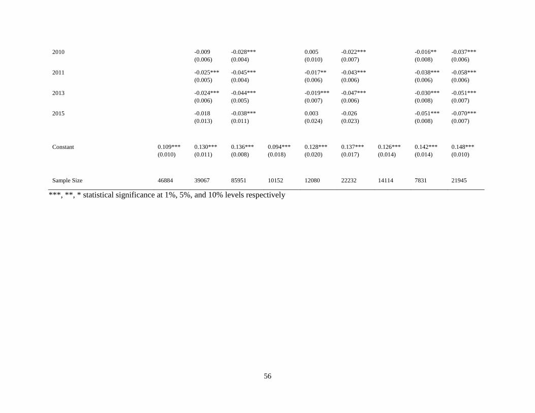
56

2010 -0.009

(0.006)

-0.028***

(0.004)

0.005

(0.010)

-0.022***

(0.007)

-0.016**

(0.008)

-0.037***

(0.006)

2011 -0.025***

(0.005)

-0.045***

(0.004)

-0.017**

(0.006)

-0.043***

(0.006)

-0.038***

(0.006)

-0.058***

(0.006)

2013 -0.024***

(0.006)

-0.044***

(0.005)

-0.019***

(0.007)

-0.047***

(0.006)

-0.030***

(0.008)

-0.051***

(0.007)

2015 -0.018

(0.013)

-0.038***

(0.011)

0.003

(0.024)

-0.026

(0.023)

-0.051***

(0.008)

-0.070***

(0.007)

Constant 0.109***

(0.010)

0.130***

(0.011)

0.136***

(0.008)

0.094***

(0.018)

0.128***

(0.020)

0.137***

(0.017)

0.126***

(0.014)

0.142***

(0.014)

0.148***

(0.010)

Sample Size 46884 39067 85951 10152 12080 22232 14114 7831 21945


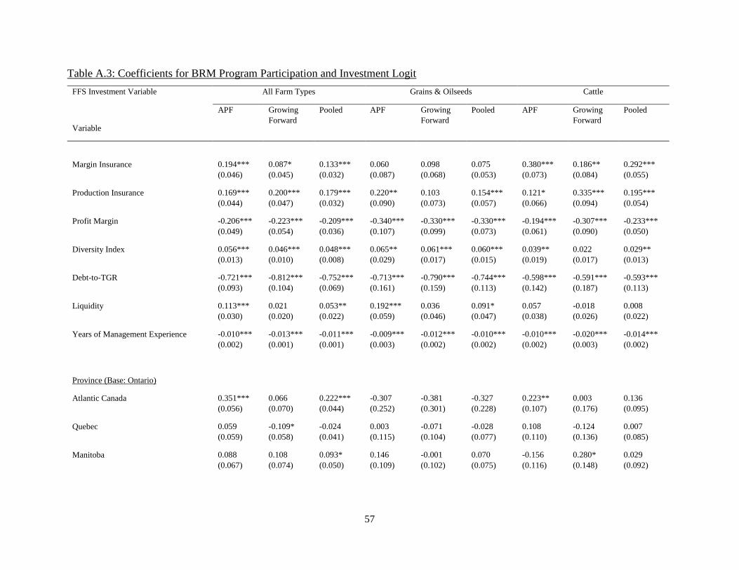
57

Table A.3: Coefficients for BRM Program Participation and Investment Logit

FFS Investment Variable All Farm Types Grains & Oilseeds Cattle

APF Growing

Forward

Pooled APF Growing

Forward

Pooled APF Growing

Forward

Pooled

Variable


(0.046)

0.087*

(0.045)

0.133***

(0.032)

0.060

(0.087)

0.098

(0.068)

0.075

(0.053)

0.380***

(0.073)

0.186**

(0.084)

0.292***

(0.055)


(0.044)

0.200***

(0.047)

0.179***

(0.032)

0.220**

(0.090)

0.103

(0.073)

0.154***

(0.057)

0.121*

(0.066)

0.335***

(0.094)

0.195***

(0.054)


(0.049)

-0.223***

(0.054)

-0.209***

(0.036)

-0.340***

(0.107)

-0.330***

(0.099)

-0.330***

(0.073)

-0.194***

(0.061)

-0.307***

(0.090)

-0.233***

(0.050)

Diversity Index 0.056***

(0.013)

0.046***

(0.010)

0.048***

(0.008)

0.065**

(0.029)

0.061***

(0.017)

0.060***

(0.015)

0.039**

(0.019)

0.022

(0.017)

0.029**

(0.013)

Debt-to-TGR -0.721***

(0.093)

-0.812***

(0.104)

-0.752***

(0.069)

-0.713***

(0.161)

-0.790***

(0.159)

-0.744***

(0.113)

-0.598***

(0.142)

-0.591***

(0.187)

-0.593***

(0.113)

Liquidity 0.113***

(0.030)

0.021

(0.020)

0.053**

(0.022)

0.192***

(0.059)

0.036

(0.046)

0.091*

(0.047)

0.057

(0.038)

-0.018

(0.026)

0.008

(0.022)


(0.002)

-0.013***

(0.001)

-0.011***

(0.001)

-0.009***

(0.003)

-0.012***

(0.002)

-0.010***

(0.002)

-0.010***

(0.002)

-0.020***

(0.003)

-0.014***

(0.002)



(0.056)

0.066

(0.070)

0.222***

(0.044)

-0.307

(0.252)

-0.381

(0.301)

-0.327

(0.228)

0.223**

(0.107)

0.003

(0.176)

0.136

(0.095)

Quebec 0.059

(0.059)

-0.109*

(0.058)

-0.024

(0.041)

0.003

(0.115)

-0.071

(0.104)

-0.028

(0.077)

0.108

(0.110)

-0.124

(0.136)

0.007

(0.085)

Manitoba 0.088

(0.067)

0.108

(0.074)

0.093*

(0.050)

0.146

(0.109)

-0.001

(0.102)

0.070

(0.075)

-0.156

(0.116)

0.280*

(0.148)

0.029

(0.092)

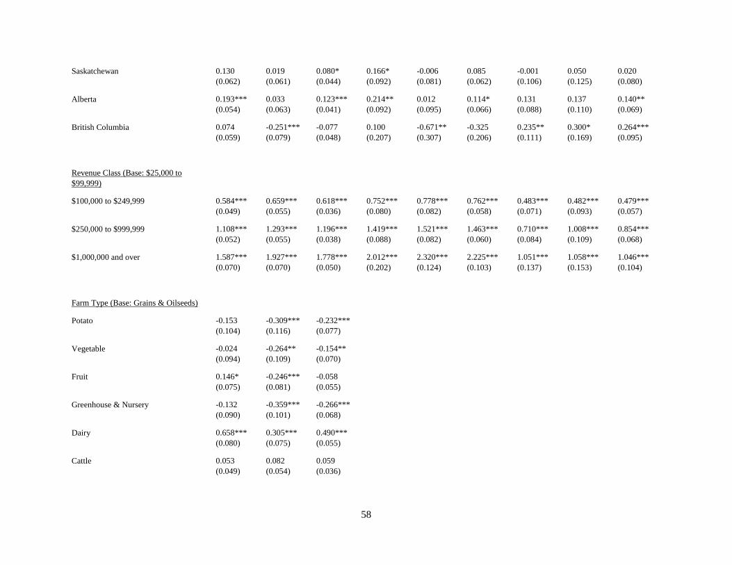
58

Saskatchewan 0.130

(0.062)

0.019

(0.061)

0.080*

(0.044)

0.166*

(0.092)

-0.006

(0.081)

0.085

(0.062)

-0.001

(0.106)

0.050

(0.125)

0.020

(0.080)

Alberta 0.193***

(0.054)

0.033

(0.063)

0.123***

(0.041)

0.214**

(0.092)

0.012

(0.095)

0.114*

(0.066)

0.131

(0.088)

0.137

(0.110)

0.140**

(0.069)

British Columbia 0.074

(0.059)

-0.251***

(0.079)

-0.077

(0.048)

0.100

(0.207)

-0.671**

(0.307)

-0.325

(0.206)

0.235**

(0.111)

0.300*

(0.169)

0.264***

(0.095)


$99,999)

$100,000 to $249,999 0.584***

(0.049)

0.659***

(0.055)

0.618***

(0.036)

0.752***

(0.080)

0.778***

(0.082)

0.762***

(0.058)

0.483***

(0.071)

0.482***

(0.093)

0.479***

(0.057)

$250,000 to $999,999 1.108***

(0.052)

1.293***

(0.055)

1.196***

(0.038)

1.419***

(0.088)

1.521***

(0.082)

1.463***

(0.060)

0.710***

(0.084)

1.008***

(0.109)

0.854***

(0.068)

$1,000,000 and over 1.587***

(0.070)

1.927***

(0.070)

1.778***

(0.050)

2.012***

(0.202)

2.320***

(0.124)

2.225***

(0.103)

1.051***

(0.137)

1.058***

(0.153)

1.046***

(0.104)


Potato -0.153

(0.104)

-0.309***

(0.116)

-0.232***

(0.077)

Vegetable -0.024

(0.094)

-0.264**

(0.109)

-0.154**

(0.070)

Fruit 0.146*

(0.075)

-0.246***

(0.081)

-0.058

(0.055)

Greenhouse & Nursery -0.132

(0.090)

-0.359***

(0.101)

-0.266***

(0.068)

Dairy 0.658***

(0.080)

0.305***

(0.075)

0.490***

(0.055)

Cattle 0.053

(0.049)

0.082

(0.054)

0.059

(0.036)

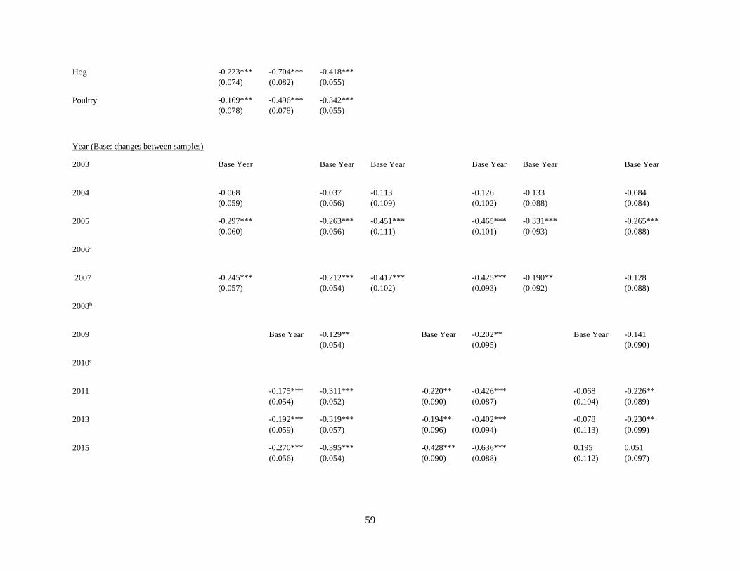
59

Hog -0.223***

(0.074)

-0.704***

(0.082)

-0.418***

(0.055)

Poultry -0.169***

(0.078)

-0.496***

(0.078)

-0.342***

(0.055)


2003 Base Year

s


2004 -0.068

(0.059)

-0.037

(0.056)

-0.113

(0.109)

-0.126

(0.102)

-0.133

(0.088)

-0.084

(0.084)

2005 -0.297***

(0.060)

-0.263***

(0.056)

-0.451***

(0.111)

-0.465***

(0.101)

-0.331***

(0.093)

-0.265***

(0.088)

2006a Sssssssssss

sss

2007 -0.245***

(0.057)

-0.212***

(0.054)

-0.417***

(0.102)

-0.425***

(0.093)

-0.190**

(0.092)

-0.128

(0.088)

2008b ssssssssssss

ss

2009 Base Year -0.129**

(0.054)

Base Year -0.202**

(0.095)

Base Year -0.141

(0.090)

2010c ssssssssssss

sss

2011 -0.175***

(0.054)

-0.311***

(0.052)

-0.220**

(0.090)

-0.426***

(0.087)

-0.068

(0.104)

-0.226**

(0.089)

2013 -0.192***

(0.059)

-0.319***

(0.057)

-0.194**

(0.096)

-0.402***

(0.094)

-0.078

(0.113)

-0.230**

(0.099)

2015 -0.270***

(0.056)

-0.395***

(0.054)

-0.428***

(0.090)

-0.636***

(0.088)

0.195

(0.112)

0.051

(0.097)

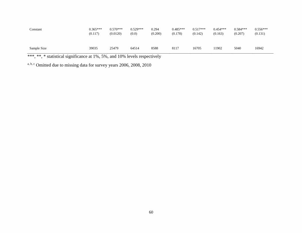
60

Constant 0.365***

(0.117)

0.570***

(0.0120)

0.529***

(0.0)

0.294

(0.200)

0.485***

(0.178)

0.517***

(0.142)

0.454***

(0.163)

0.584***

(0.207)

0.556***

(0.131)

Sample Size 39035 25479 64514 8588 8117 16705 11902 5040 16942


a, b, c Omitted due to missing data for survey years 2006, 2008, 2010

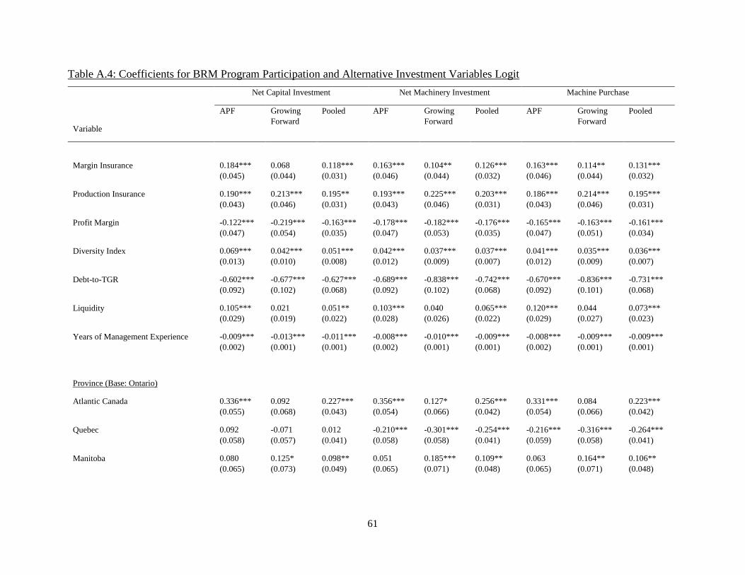
61

Table A.4: Coefficients for BRM Program Participation and Alternative Investment Variables Logit

Net Capital Investment Net Machinery Investment Machine Purchase

APF Growing

Forward

Pooled APF Growing

Forward

Pooled APF Growing

Forward

Pooled

Variable


(0.045)

0.068

(0.044)

0.118***

(0.031)

0.163***

(0.046)

0.104**

(0.044)

0.126***

(0.032)

0.163***

(0.046)

0.114**

(0.044)

0.131***

(0.032)


(0.043)

0.213***

(0.046)

0.195**

(0.031)

0.193***

(0.043)

0.225***

(0.046)

0.203***

(0.031)

0.186***

(0.043)

0.214***

(0.046)

0.195***

(0.031)


(0.047)

-0.219***

(0.054)

-0.163***

(0.035)

-0.178***

(0.047)

-0.182***

(0.053)

-0.176***

(0.035)

-0.165***

(0.047)

-0.163***

(0.051)

-0.161***

(0.034)

Diversity Index 0.069***

(0.013)

0.042***

(0.010)

0.051***

(0.008)

0.042***

(0.012)

0.037***

(0.009)

0.037***

(0.007)

0.041***

(0.012)

0.035***

(0.009)

0.036***

(0.007)

Debt-to-TGR -0.602***

(0.092)

-0.677***

(0.102)

-0.627***

(0.068)

-0.689***

(0.092)

-0.838***

(0.102)

-0.742***

(0.068)

-0.670***

(0.092)

-0.836***

(0.101)

-0.731***

(0.068)

Liquidity 0.105***

(0.029)

0.021

(0.019)

0.051**

(0.022)

0.103***

(0.028)

0.040

(0.026)

0.065***

(0.022)

0.120***

(0.029)

0.044

(0.027)

0.073***

(0.023)


(0.002)

-0.013***

(0.001)

-0.011***

(0.001)

-0.008***

(0.002)

-0.010***

(0.001)

-0.009***

(0.001)

-0.008***

(0.002)

-0.009***

(0.001)

-0.009***

(0.001)



(0.055)

0.092

(0.068)

0.227***

(0.043)

0.356***

(0.054)

0.127*

(0.066)

0.256***

(0.042)

0.331***

(0.054)

0.084

(0.066)

0.223***

(0.042)

Quebec 0.092

(0.058)

-0.071

(0.057)

0.012

(0.041)

-0.210***

(0.058)

-0.301***

(0.058)

-0.254***

(0.041)

-0.216***

(0.059)

-0.316***

(0.058)

-0.264***

(0.041)

Manitoba 0.080

(0.065)

0.125*

(0.073)

0.098**

(0.049)

0.051

(0.065)

0.185***

(0.071)

0.109**

(0.048)

0.063

(0.065)

0.164**

(0.071)

0.106**

(0.048)

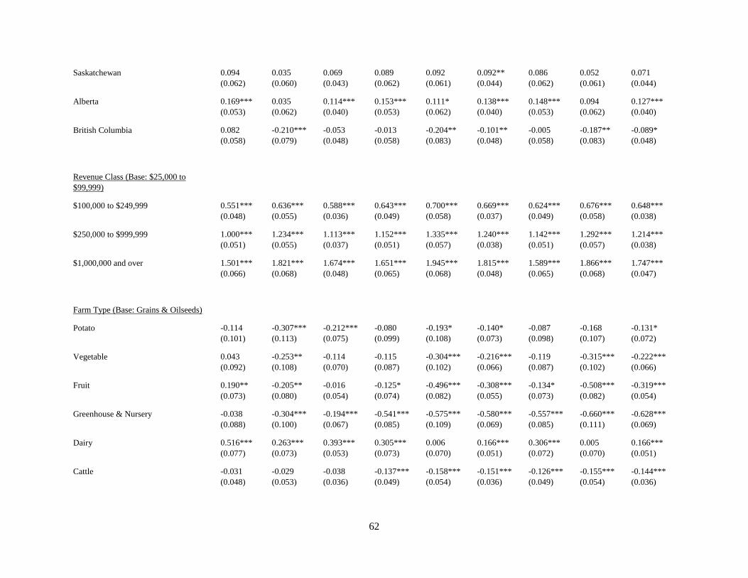
62

Saskatchewan 0.094

(0.062)

0.035

(0.060)

0.069

(0.043)

0.089

(0.062)

0.092

(0.061)

0.092**

(0.044)

0.086

(0.062)

0.052

(0.061)

0.071

(0.044)

Alberta 0.169***

(0.053)

0.035

(0.062)

0.114***

(0.040)

0.153***

(0.053)

0.111*

(0.062)

0.138***

(0.040)

0.148***

(0.053)

0.094

(0.062)

0.127***

(0.040)

British Columbia 0.082

(0.058)

-0.210***

(0.079)

-0.053

(0.048)

-0.013

(0.058)

-0.204**

(0.083)

-0.101**

(0.048)

-0.005

(0.058)

-0.187**

(0.083)

-0.089*

(0.048)


$99,999)

$100,000 to $249,999 0.551***

(0.048)

0.636***

(0.055)

0.588***

(0.036)

0.643***

(0.049)

0.700***

(0.058)

0.669***

(0.037)

0.624***

(0.049)

0.676***

(0.058)

0.648***

(0.038)

$250,000 to $999,999 1.000***

(0.051)

1.234***

(0.055)

1.113***

(0.037)

1.152***

(0.051)

1.335***

(0.057)

1.240***

(0.038)

1.142***

(0.051)

1.292***

(0.057)

1.214***

(0.038)

$1,000,000 and over 1.501***

(0.066)

1.821***

(0.068)

1.674***

(0.048)

1.651***

(0.065)

1.945***

(0.068)

1.815***

(0.048)

1.589***

(0.065)

1.866***

(0.068)

1.747***

(0.047)


Potato -0.114

(0.101)

-0.307***

(0.113)

-0.212***

(0.075)

-0.080

(0.099)

-0.193*

(0.108)

-0.140*

(0.073)

-0.087

(0.098)

-0.168

(0.107)

-0.131*

(0.072)

Vegetable 0.043

(0.092)

-0.253**

(0.108)

-0.114

(0.070)

-0.115

(0.087)

-0.304***

(0.102)

-0.216***

(0.066)

-0.119

(0.087)

-0.315***

(0.102)

-0.222***

(0.066)

Fruit 0.190**

(0.073)

-0.205**

(0.080)

-0.016

(0.054)

-0.125*

(0.074)

-0.496***

(0.082)

-0.308***

(0.055)

-0.134*

(0.073)

-0.508***

(0.082)

-0.319***

(0.054)

Greenhouse & Nursery -0.038

(0.088)

-0.304***

(0.100)

-0.194***

(0.067)

-0.541***

(0.085)

-0.575***

(0.109)

-0.580***

(0.069)

-0.557***

(0.085)

-0.660***

(0.111)

-0.628***

(0.069)

Dairy 0.516***

(0.077)

0.263***

(0.073)

0.393***

(0.053)

0.305***

(0.073)

0.006

(0.070)

0.166***

(0.051)

0.306***

(0.072)

0.005

(0.070)

0.166***

(0.051)

Cattle -0.031

(0.048)

-0.029

(0.053)

-0.038

(0.036)

-0.137***

(0.049)

-0.158***

(0.054)

-0.151***

(0.036)

-0.126***

(0.049)

-0.155***

(0.054)

-0.144***

(0.036)

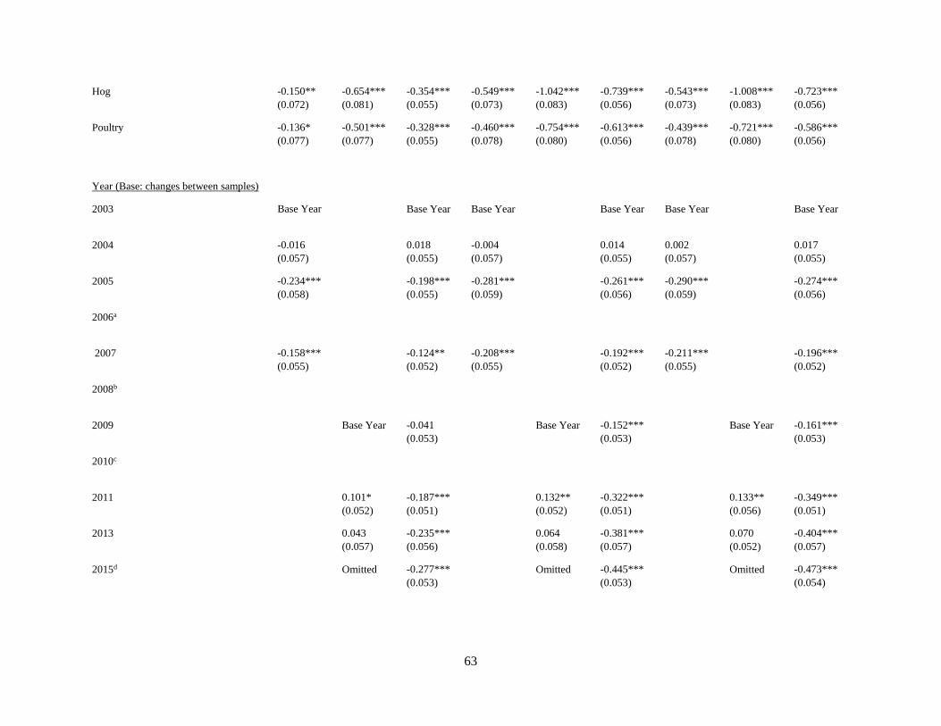
63

Hog -0.150**

(0.072)

-0.654***

(0.081)

-0.354***

(0.055)

-0.549***

(0.073)

-1.042***

(0.083)

-0.739***

(0.056)

-0.543***

(0.073)

-1.008***

(0.083)

-0.723***

(0.056)

Poultry -0.136*

(0.077)

-0.501***

(0.077)

-0.328***

(0.055)

-0.460***

(0.078)

-0.754***

(0.080)

-0.613***

(0.056)

-0.439***

(0.078)

-0.721***

(0.080)

-0.586***

(0.056)


2003 Base Year

s


2004 -0.016

(0.057)

0.018

(0.055)

-0.004

(0.057)

0.014

(0.055)

0.002

(0.057)

0.017

(0.055)

2005 -0.234***

(0.058)

-0.198***

(0.055)

-0.281***

(0.059)

-0.261***

(0.056)

-0.290***

(0.059)

-0.274***

(0.056)

2006a Sssssssssss

sss

2007 -0.158***

(0.055)

-0.124**

(0.052)

-0.208***

(0.055)

-0.192***

(0.052)

-0.211***

(0.055)

-0.196***

(0.052)

2008b Sssssssssss

sss

2009 Base Year -0.041

(0.053)

Base Year -0.152***

(0.053)

Base Year -0.161***

(0.053)

2010c Sssssssssss

ssss

2011 0.101*

(0.052)

-0.187***

(0.051)

0.132**

(0.052)

-0.322***

(0.051)

0.133**

(0.056)

-0.349***

(0.051)

2013 0.043

(0.057)

-0.235***

(0.056)

0.064

(0.058)

-0.381***

(0.057)

0.070

(0.052)

-0.404***

(0.057)

2015d Omitted -0.277***

(0.053)

Omitted -0.445***

(0.053)

Omitted -0.473***

(0.054)

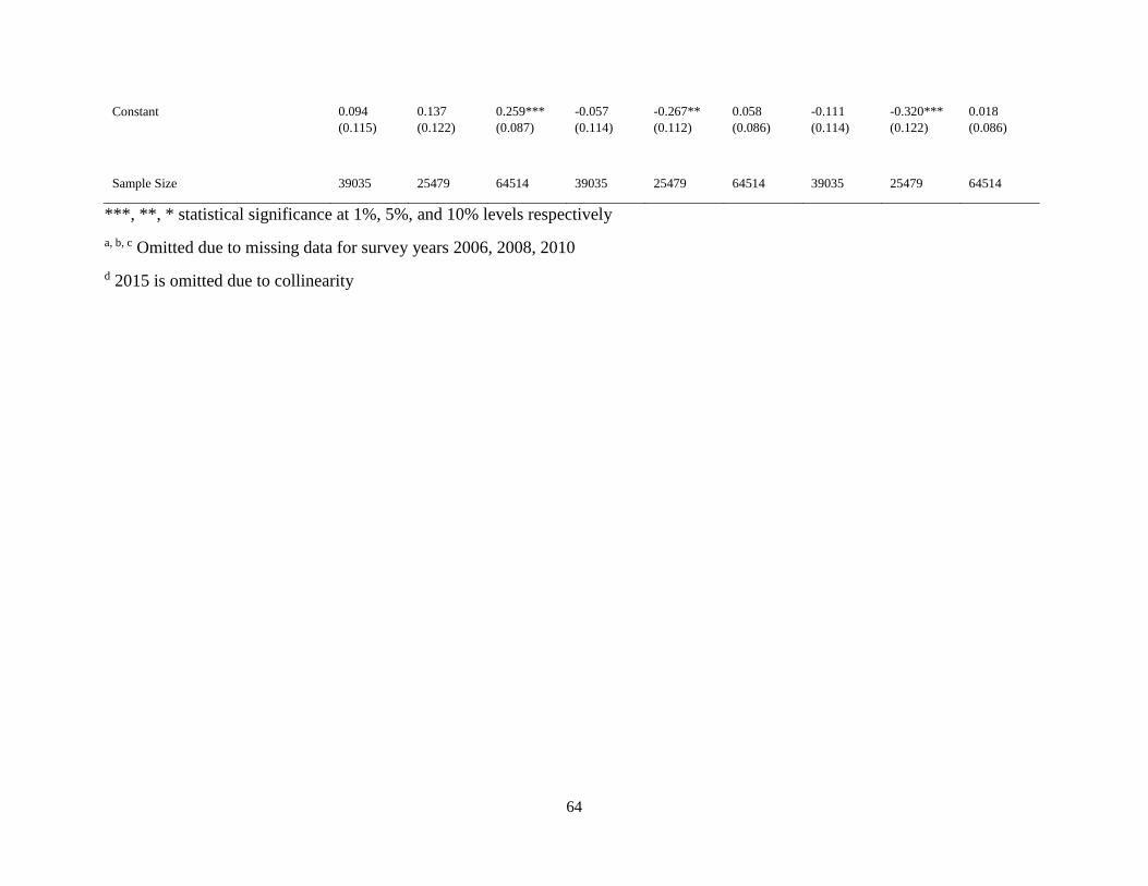
64

Constant 0.094

(0.115)

0.137

(0.122)

0.259***

(0.087)

-0.057

(0.114)

-0.267**

(0.112)

0.058

(0.086)

-0.111

(0.114)

-0.320***

(0.122)

0.018

(0.086)

Sample Size 39035 25479 64514 39035 25479 64514 39035 25479 64514


a, b, c Omitted due to missing data for survey years 2006, 2008, 2010

d 2015 is omitted due to collinearity

Documents

BUSINESS RISK MANAGEMENT PROGRAMS AND ON-FARM …