Breaking in New Markets:

Relying on Networks or Spillovers? ∗

Shibi He†

Volodymyr Lugovskyy‡

August 1, 2019

Abstract

Exporting firms have been shown to use various channels—spillovers, networks, and se-

quential entry—of alleviating risk and uncertainty when breaking into new markets. Pre-

vious literature studied these channels in isolation and did not examine the importance

of the supplier network (SN) channel. Using several firm-level datasets on exporting and

importing, we construct novel, highly disaggregated, measures of (i) spillover combined

with sequential entry (Spillover/SE), (ii) consumer exports network (CEN), (iii) SN, and

jointly estimate their effects on breaking in new markets. We show that the SN is the

most important channel for the exporters with one export destination. Thus, any trade

barriers affecting the extensive margin of imports have an adverse effect on the exten-

sive margin of exports, especially by smaller exporters. Overall, the SN is as important

as Spillover/SE channel with the CEN having a somewhat smaller effect. Importantly,

omitting any of these channels biases (upwards) the marginal effects of other channels by

up to 150%. For a subset of our data, we are able to construct an even more granular,

firm-to-firm, measure of the CEN. It has a three times higher effect (on breaking in new

markets) than a more aggregate, firm-to-country, measure, which confirms the impor-

tance of direct contacts emphasized by the networks literature.

Keywords: Firm-level, Spillover, Networks, Trade.

JEL Classification Number: F1, L14

∗We thank Felipe Benguria, Ahmad Lashkaripour, Emerson Melo, James Rauch, Alexandre Skiba and theparticipants of the 2019 Spring Midwest Trade Meetings for helpful comments.†Department of Economics, Indiana University, Wylie Hall, 100 S. Woodlawn, Bloomington, IN 47405-7104;

e-mail: shibhe@indiana.edu‡Department of Economics, Indiana University, Wylie Hall Rm 301, 100 S. Woodlawn, Bloomington, IN

47405-7104; e-mail: vlugovsk@indiana.edu

1

1 Introduction

Breaking in new markets is critical for export diversification and economic growth since it

enhances country’s ‘self-discovery’ (Hausmann and Rodrik, 2003),1 and a substantial frac-

tion of aggregate exports is generated by new exports (Eaton et al., 2014; Bernard et al.,

2009; Lawless, 2009; Albornoz et al., 2016). Entering new markets, however, is subject to

sizable information uncertainty and risk. To alleviate these obstacles, firms employ various

channels. For example, they study the exports of other domestic firms—domestic spillovers

(Greenaway et al., 2004; Silvente and Gimenez, 2007; Koenig et al., 2010); leverage their own

experiences—sequential exporting (Bernard and Jensen, 2004; Eaton et al., 2009; Albornoz

et al., 2012; Nguyen, 2012); and search remotely from their customer’s locations—network

remote search (Chaney, 2014; He, 2018).

While this is literature is growing, some important questions are still unanswered. First,

there is no consensus on whether spillovers have an effect on breaking in new markets. While

some researchers find the effect to be substantial (Silvente and Gimenez, 2007; Koenig, 2009;

Koenig et al., 2010; Choquette and Meinen, 2015),2 others claim it to be negligible (Bernard

and Jensen, 2004). Second, the related network literature focused mainly on the consumer

exports networks (CENs) (e.g., Chaney, 2014), while the effect of supplier networks (SNs)

is yet to be explored (as pointed out by Bernard and Moxnes, 2018). Third, the effects of

spillovers, sequential entry, and networks have been studied in isolation. Their relative im-

portance is unknown and the existing estimates might be subject to the omitted variables

bias. This paper attempts to fill these gaps.

To this goal, we use matched Colombian exports and imports firm-level datasets, along with

Chilean imports and exports data, and several other datasets. The exact network of infor-

mational flows leading to a certain exporting outcome can be complex and, with exception of

controlled settings of field experiments (e.g., Atkin et al., 2017), is impossible to trace since

the data on information gathering and decision making by managers is hardly available. Ev-

ery network, however, simple or complex, consists of links. Our approach is built on tracing

the most granular observable informational links and examining which of them increase the

probability of exporting to new and existing destinations. First, for each Colombian export-

ing firm and potential export destination, we check whether other Colombian firms export

1Under information uncertainty a country’s comparative advantage is not evident and has to be discoveredthrough trial and error. Hausmann and Rodrik (2003) rank the country’s self-discovery through exporting asthe most important factor for economic growth—even above reducing corruption and getting access to foreigntechnology.

2It also includes examples of how practitioners facilitate information exchange between current and poten-tial exporters at various conferences and gatherings (e.g., Koenig et al., 2010).

2

to this destinations products which this firm has shown a potential to export. We label this

type of links as the spillover combined with sequential entry (henceforth, Spillover/SE) link.

Second, inspired by Chaney (2014) and Bernard and Moxnes (2018), we focus on two types of

links related to the firm-to-country networks: consumer exports network (CEN) and supplier

network (SN).3 The CEN link identifies countries to which firms from my current export

destinations export their products. The SN link identifies the countries of my suppliers.

Using these constructed links, we are the first to jointly estimate the effects of Spillover/SE,

CEN, and SN links on the probability of firm’s breaking in a new market. We find that (i)

the SN links are at least as important as the CEN links, (ii) the SN and CEN links combined

are at least as important as the Spillover/SE links, and (iii) the omission of either CEN, SN,

or Spillover/SE links generates a pronounced (up to 120%) upward bias for other links. By

matching Colombian exporters with their partnering Chilean importers, we are also able to

construct a more granular, firm-to-firm, measure of the CEN links, which traces the exports

of the Colombian trading partners (rather than of all firms as in firm-to-country CEN) in

Chile. We find that these firm-to-firm links have an up to three times stronger effect (on

breaking in new markets) than a more aggregate, firm-to-country, measure of CEN links.

For our first empirical exercise, we use Colombian Exports and Imports transaction-level

data and United Nations Comtrade worldwide trade data, for years 2007-2016. Our depen-

dent variable is defined from the perspective of Colombian exporting firms and it has three

dimensions: firm, export destination (country), and year. It is one if Colombian firm i ex-

ports to country c in year t, and zero otherwise. Similarly to Chaney (2014), we employ

a dynamic Probit model to examine factors affecting firm’s export destinations. Our main

variables of interest are: Spillover/SE dummy, firm-to-country CEN dummy, and SN dummy.

We propose novel ways of constructing these variables, which allow us to utilize data at

firm-product-destination-year level, but to maintain the manageable size of the dataset. The

Spillover/SE for firm i country c year t is set to one if, in year t − 1, any other Colom-

bian firm exported at least one of the products (defined at Harmonized System 6-digit level)

exported by i to any country in year t and zero otherwise. Thus, Spillover/SE dummy sum-

marizes information about products exported by firm i in year t − 1 and about wether any

of these products were exported by other Colombian firms to a given country in year t− 1.4

3While our construction of the CEN measure is different from that of Chaney (2014), it is in line withhis idea of export networks. Bernard and Moxnes (2018) indicated that the analysis of supplier networks ismissing in this literature.

4Its coefficient as well as coefficients of other dummy variables can be interpreted as the effect of thisvariable on the expansion to new destinations, since as in Chaney (2014), all specifications include a dummyvariable of exporting to a given destination in the previous year, which controls for the continuing exports to

3

Previous studies defined spillovers at more aggregate level—often a single-dimensional one

(e.g., Bernard and Jensen, 2004). Combining Spillovers and SE into one variable allows us

to have only one observation per firm-destination-year instead of one observation per firm-

destination-year-product, which decreases the required number of observations to only 16.9

mln instead of 85 bln.

To construct the firm-to-country CEN dummy variable for each Colombian firm, we first

identify the set of export destinations (countries) for each firm i. For firm i and country c,

the CEN dummy is equal to one if i’s export destinations export to country c within the same

industry as they import from i.5 Finally, the SN dummy is introduced to examine whether

firms may find new customers in the countries of their foreign suppliers. We also comple-

mented the constructed set of dummies with the standard control variables used by Chaney

(2014), i.e., geographic proximity measures, import and export growth rates, and market size.

We find the coefficients for all three variables to be both statistically and and economically

significant and of the right sign. The marginal effect of the Spillovers/SE, CEN, and SN are

more important than the marginal effects of all control variables, such as geographic proxim-

ity measures, import and export growth rates, and market size, combined.6 Importantly, we

can rank the marginal effects of the Spillover/SE, CEN, and SN, and to demonstrate that

omitting either of the channels generates pronounced upward bias for other effects. These

findings are important, since they show that evidence based on the micro data provide strong

support for spillover and networks—including foreign supplier networks—effects in exporting

to new markets.

For our next step, we combine three transaction-level datasets for years 2007-2016: Colom-

bian Exports, Chilean Imports, and Chilean Exports. We utilize the fact that Colombian

Exports dataset includes the identity of both exporting and (foreign) importing firms. This

enables us to match Colombian exporting firms with their Chilean importing counterparts

in each year between 2007 and 2015. To control for the sequential exporting and potential

networks through other export destinations, we restrict our sample to the Colombian firms

which originally export only to Chile. For firm i and country c, the firm-to-firm CEN dummy

is equal to one if i’s trading partners (i.e., Chilean importing firms) export to country c within

a given destination.5To construct this variable, we employ the worldwide bilateral trade at product level from the United

Nations Comtrade dataset.6The choice of our control variables was motivated by the specifications of Chaney (2014) plus we added

an adjacency dummy variable to control for the similarity between an exporting firm’s home country and thepossible export destination as suggested by Rauch (2001). We do not have production data for Colombia, andthus we cannot use data on plant size, employment and wages as in Bernard and Jensen (2004).

4

the same industry as they import from i.7 All other variables are constructed in the same

fashion as in the previous exercise.

Our main result is that, within the same sample, the marginal effect of the firm-to-firm CEN

is two to three times greater than that of the firm-to-country CEN. That is, Colombian firms

are much more likely to utilize the information obtained from their trading partners in Chile

than from observing where other Chilean firms export. Put differently, the more granular

is the observed information channel, the greater is the predictive power of this information.

Importantly, both Spillovers/SE and the CEN effects are statistically and economically sig-

nificant even for the less advanced exporters—recall that we focus on firms which originally

export to only one country (Chile) and tend to have very few, on average 1.5, trading part-

ners in Chile.8 Our evidence thus present an even stronger support for the importance of

spillovers and networks for firm’s expansion path.

Furthermore, focusing on firms with a single trade partner allowed to downplay additional,

more complex effects present in larger networks, such as reputation effects, homophile9, segre-

gation, etc.10 For example, a firm with multiple trading partners is potentially likely to have

a stronger reputation in the eyes of the potential new partners, as multiple trading partners

project higher quality and reliability than a firm with only few partners. Thus, even if a firm

meets a new partner without direct involvement of the existing partner, being a part of the

larger network might have facilitated the match. Focusing on firms with a minimal network

allowed us to isolate these effects.

The rest of the paper is organized as follows. Section 2 discusses related literature. Section 3

provides a detailed data description. Section 4 presents empirical models and the estimation

results. Section 5 provides robustness checks. Section 6 concludes.

2 Related Literature

This paper contributes to several strands of literature. Most directly, it adds to a large lit-

erature on firms’ expansion in international markets. The existing literature has identified

three strategies that firms use to expand into new markets: domestic information spillover,

7To construct this variable, we matched firms and industries in Chilean Imports and Chilean Exportsdatasets.

8As demonstrated by Chaney (2014), these firms are least likely to expand, as their networks are minimal.9The widely known analog of homophily effect in trade is Linder effect—firms are more likely to export to

countries with the similar income per capita as the one in their own country.10See, for example, Currarini et al. (2009) and Jackson and Zenou (2015) for a more detailed description of

these and other additional effects in larger social networks.

5

foreign networks, and sequential exporting.

The literature on domestic spillovers is the largest among the three. It emphasizes the pool

of existing exporters as an important source of information for other firms (Koenig et al.,

2010). Firms tend to learn about profits, requirements, and challenges in the overseas mar-

kets by observing other firms’ exporting experience, and they tend to imitate the export

behavior of the more successful, more experienced leaders. Clerides et al. (1998), Silvente

and Gimenez (2007), Koenig (2009), Koenig et al. (2010), and Choquette and Meinen (2015)

used firm-level data from different countries to show that a firm’s export decision and/or the

volume exported by the firm are positively affected by their neighboring firms11. Aitken et al.

(1997), Greenaway et al. (2004), and Kneller and Pisu (2007) identified multinationals as one

of the most important sources of information spillover. Iacovone and Javorcik (2010) used

Mexican export data to show that once a firm begins exporting a new product, other firms

will soon export the same products. Wagner and Zahler (2015) explored detailed data on new

exporters in Chile and found that followers are 40% more likely to enter a product if a pio-

neer survives more than one year of exporting that product. Bernard and Jensen (2004), on

the other hand finds the effects of domestic spillovers on export entry by other firms negligible.

Our contribution to this literature is twofold. First, when examining the spillover effects, we

control for other important effects, including network and sequential-export effects. Second,

we were able to rank the magnitude of the spillover effect versus other effects. Overall, the

Spillover/SE effect has the same marginal effect on the probability of entering anew market

as the SN effect with both effects dominating the CEN effect. When experimenting with

subsamples of firms with different number of export destinations, we found that SN is more

important than the Spillover/SE for Colombian firms exporting to only one destination, while

the opposite is true for firms exporting to between two and five and to more than five des-

tinations. Finally, omitting the spillover effect in the empirical specification leads to very

pronounced upward biases of other effects, while omitting network effects and common lan-

guage substantially biases the Spillover/SE effect.

The literature on networks and trade dates back to Rauch (1999), who introduced the idea

that informational frictions dampen trade, and that social networks between buyers and sell-

ers help reducing these frictions and promote trade12. While a more recent strand of the

11There is also theoretical and empirical literature on the negative effect of spillovers on firms’ exportdecisions. For example, Ciliberto and Jakel (2017) documented the negative effects of present competitors onforeign market entry, but they only focus on the superstar exporters. Barrios et al. (2003) and Bernard andJensen (2004) found no evidence of spillover effects on firms’ decisions to export, but they didn’t address theexpansion to new markets for firms that already export.

12See also Rauch (2001), Chaney (2016), and Bernard and Moxnes (2018) for excellent surveys on networks

6

literature empirically estimates the trade-creating effect of networks using country-specific

case studies,13 it is relatively silent on the expansion path at the firm level.

Do exporting firms rely on their networks of existing trade partners to search for new trade

partners? This question was answered positively by Chaney (2014, 2018). Theoretically, both

papers modeled the remote search for new partners through existing trading partners. Em-

pirically, Chaney (2014) provided the reduced-form evidence of the effect of firm-to-country

networks on the export expansion path of French firms. Building on Chaney(2014)’s work, we

provide an additional test of the effect of the consumer export networks on trade expansion

by using a finer firm-to-firm measure of networks of Colombian and Chilean firms. We show

that firm-to-firm CENs do have a positive effect on the choice of new export destinations

even after controlling for the spillover and sequential-exporting effects. Quantitatively, we

show that a Colombian firm’s probability of choosing a new export destination would increase

by 55% (from 0.0022 to 0.0034) if its Chilean trade partners exported the same HS 2-digit

product to that country in the previous period.

We also shed some light on the role of the foreign supplier networks on finding new export

destinations. While the literature on foreign supplier networks is quite extensive, it tends to

focus on other aspects of networks, such as propagation of shocks (Barrot and Sauvagnat,

2016; Lim, 2018), firm performance (Bernard et al., 2018b), firm’s exposure to trade through

its domestic network (Tintelnot et al., 2018), etc. We show that SN is one of the two most

important channels for breaking in new markets in the entire sample, whereas has by far the

greatest marginal effect among the firms with only one export destination. Furthermore, not

including SN in the estimation equation generates a substantial upward bias for other effects.

Our paper is also related to a new but flourishing literature that focuses on the firm-to-firm

connections in international trade. The vast majority of world trade flow is between firms.

However, many empirical studies are restricted to aggregated trade, due to the scarcity of

the detailed trade transaction data between firms. Recently, with the increasing availability

of firm-to-firm trade data, the literature has started to explore the role of the connections be-

tween individual exporters and importers. For example, Rauch and Watson (2004), Antras

and Costinot (2011), Petropoulou (2008), and Chaney (2014) modeled intermediaries as

agents that facilitate matching between exporters and foreign buyers. Benguria (2015) pro-

posed a model to analyze the sorting and matching between exporting and importing firms

and trade.13Rauch and Trindade (2002), Combes et al. (2005), Greaney (2009), Garmendia et al. (2012), and Aleksyn-

ska and Peri (2014) while using different methodologies and/or datasets, arrive at the same conclusion thatthe cultural, social, and business networks can largely facilitate international trade.

7

and provides empirical evidence in support of this theory. Other papers have examined the

cross-section and/or evolution of firm-to-firm connections in trade (Eaton et al., 2009; Blum

et al., 2010, 2012; Bernard et al., 2014, 2018a; Dragusanu, 2014; Monarch, 2014). We show

that these connections are critical for a firm’s choice of new export destinations.

Our paper also contributes to the Hausmann and Rodrik (2003)’s influential hypothesis of

suboptimal exporting due to missing export pioneers. In sectors with latent comparative

advantage, pioneering activity is both risky and costly, while benefits are dispersed also among

the followers, which benefits from observing the performance of pioneers. In fact, as shown

by Wagner and Zahler (2015), followers tend to overtake export flows from pioneers within a

relatively short period of time. This externality feature of pioneering results in the suboptimal

pioneering, especially, for smaller countries (Wei et al., 2017). We classify Colombian export

pioneers into global—those which are the first to export a product from Colombia—and

market-specific—those which are the first to export a product to a certain market. Since we

explicitly control for export followers by Spillover/SE, the marginal effects of CEN and SN

can be interpreted as the increase in probability of market-specific pioneering. We are the

first to show, that among the two, the SN has a more pronounced effect, especially among

the firms with only one export destinations. Importantly, among all considered channels, the

CEN and SN seem to be the major channels enhancing market-specific pioneering.

3 Data

Our primary data source is the customs records of Colombian and Chilean import and export

transactions between 2007 and 2016.14 A transaction record includes the firm’s national tax

ID number, the product code at Harmonized System (HS) 10-digit level,15 the value of the

transaction in US dollars, the country of destination for export data, and the country of

origin for import data. For our first set of regressions, we will use the entire sample, which

we will denote as Full Sample.

For our second set of regressions, with the the firm-to-firm measure of networks, we will

use the Restricted Sample. In this set of regressions, we utilize an important feature of the

Colombian export data: for each export transaction, we also observe the names of foreign

importing firms. This allows us to identify Chilean firms that import from Colombia, and to

focus on Colombian exporters which initially export only to Chile.16 This allows us to trace

14The data is obtained from Datamyne, a company that specializes in documenting import and exporttransactions in Americas. For more detail please see www.datamyne.com.

15In our paper we need the product dimension only for the Colombian part of the data, which is at HS10.16The names of these Chilean firms are not standardized in the Colombian exports data. There are in-

stances in which the name of the same firm and its address are recorded differently (e.g., using abbreviations,

8

the export destinations of the direct Chilean partners of Colombian firms. In what follows,

we explain and motivate the construction of variables used in our analysis.

3.1 Dependent Variable: Entry

Following Chaney (2014), our dependent variable, Entryi,c,t+1, is set to one if, conditional

on being an exporter in year t, firm i exports to country c in year t+ 1, and zero otherwise.

In what follows we will explain sample dimensions for Full and Restricted samples.

Full Sample. Exploring Colombian transaction-level export data, we identified 91,891

firm-year combinations of Colombian exporting firms between 2007 and 2015. To con-

struct Entryi,c,t+1, we considered 184 countries that we have information on distance and

size as potential exporting destinations for each firm, which gave us a total of 16,907,944

(= (91, 891 firm-year obs.)× (184 countries)) possible firm-year-destination combinations.

Restricted Sample. To examine the effects of the firm-to-firm measure of networks, we

restrict our sample to the Colombian firms that initially export only to Chile and within

this sample define the Entry variable the same as above. Using Colombian and Chilean

transaction-level export and import data, we successfully matched 577 Colombian firms (163

expanding firms, 119 non-expanding firms, and 295 disappearing firms) to their Chilean

importing counterparts. For each of these matched Colombian firms, we define the Entry

dummy, Entryi,c,t+1, to be equal to one if, conditional on exporting only to Chile in year t,

it exported to country c in year t+ 1, and zero otherwise. We considered 183 countries (184

countries minus Chile) as potential new export destinations for matched Colombian firms,

which gave us a total of 105,591 (=(577 firm-year obs.) × (183 countries)) possible firm-year-

destination combinations. As shown in the first column of Table C.1, we found that Entry

dummy equals one for 237 of these combinations, suggesting that conditional on expanding,

a firm that previously exported only to Chile will export, on average, to 237/163=1.5 new

destinations.

3.2 Independent Variables

Spillover/Sequential Exporting Dummy. We constructed a Spillover/Sequential Ex-

porting dummy variable, Spillover/SEi,c,t, to examine how the choice of new export des-

tination is affected by both spillovers and sequential exporting effects. For each exporting

firm i, we first identified which HS 6-digit products were exported by the firm at time t.

dots, dashes, extra spaces, etc.). We deal with this problem by standardizing the spelling of the names andby comparing these names to the standardized names of firms in the Chilean imports data. The detaileddescription of cleaning the exporters’ names is provided in the Appendix A.

9

We then explored the Colombian transaction-level export data to see if there was any other

Colombian firm j exporting at least one of these products at time t to country c. If yes,

Spillover/SEi,c,t, was set to one for c and if no, it was set to zero.

Note that our Spillover/SE is constructed at product-country level, whereas previous liter-

ature defines it at industry-country or even industry-‘export status’ levels. This potentially

could have increased the sample size by several orders of magnitude since we are considering

over 5000 HS6 products. If we were to consider for spillovers separately from sequential en-

try (i.e., whether any Colombian firm exported this product to a given country) the sample

would have increased from 16.9 mln to over 100 bln. Thus, combining both effects together

makes the sample size more manageable.17

Consumer Export Network: Firm-to-Country and Firm-to-Firm Measures. We

constructed a firm-to-country measure of Consumer Export Network dummy variable ExpNetworki,c,t,

to examine whether Colombian exporting firms rely on their current exporting destinations

to remotely search for new destinations. Consider a Colombian firm i exporting product(s)

within industry Z18 in year t to a certain set of countries X. The Consumer Export Network

dummy, ExpNetworki,c,t, equals one for all destination c to which any of these countries in

X exports products within the same industry Z in year t, and zero otherwise. In our exercise

with Colombian exports to Chile only (Restricted Sample), the set X contains a single country

Chile. Thus, the firm-to-country measure of ExpNetworki,c,t, equals one for all destinations

to which Chile exports products within the same industry Z at time t, and zero otherwise.

For a more granular, firm-to-firm measure of the CEN, we matched Colombian exporting

and Chilean importing firms, along with the additional transaction dataset on Chilean ex-

ports. For each of the 577 matched Colombian firms, the firm-to-firm network dummy,

ExpNetworki,c,t, equals one for each destination c to which any of its matched Chilean im-

porting firms exports (within the same industry) and zero otherwise.

Supplier Import Network Dummy. Firms may learn about new export destinations

through their foreign suppliers. To examine this possibility, we matched firms in Colombian

exports and imports datasets and constructed a Supplier Import Network dummy variable,

ImpNetworki,c,t. For each Colombian exporting firm, ImpNetworki,c,t is set to one for each

country c from which the firm imports and to zero otherwise.

17Importantly, firms tend to expand with products which they previously exported. For example, in ourRestricted Sample, more than 83% of Colombian expanding firms expanded with HS 6-digit product(s) thatthey previously exported to Chile, suggesting a strong consistency in the products exported by Colombianfirms over time.

18Consumer Export Network Dummy variable is HS 2-digit specific.

10

Adjacency Dummies. Muendler and Rauch (2018) pointed out that the literature on ex-

port spillover and network search is subject to the problem of correlated unobservables. That

is, a firm may enter a new market not necessarily because it learnt about it through spillover

or network channels, but because that market is similar to the firms’ previous export des-

tinations or its home country. The use of firm-to-firm measure of networks helps us resolve

this problem when estimating the network effect, since all firms initially export to only one

market (Chile) and network search can be attributed only to export destinations of firm’s

trading partners in Chile.

The problem still potentially exists for the spillover channel. Firms entering the same mar-

ket as other firms in the same industry might not be caused by the information spillover,

but rather by the market’s similarities or adjacency to the home country. To address this

concern, we included an adjacency dummy variable to our empirical specifications to control

for the similarity between Colombia and the potential new exporting destination. Following

Morales et al. (2014) and Muendler and Rauch (2018), adjacency is defined in four different

ways: Languagec, Contiguityc, Continentc, and IncomeGroupc. These variables are defined

as indicators taking the value of one when Colombia shares a border, an official language, a

continent, and the same income group (World Bank’s classification for calender year 2007),

respectively, with a firm’s potential new export destination c. We include the adjacency

dummy Languagec in our baseline estimation, the other three adjacency variables are dis-

cussed in the robustness check section.

Other Variables. Following Chaney (2014), we also used eight additional variables to

control for geographic proximity, import sources, market size, export and import growth,

and previous export status.

(i) Ncontactsi,t controls for the number of countries to which firm i currently exports, i.e.

the number of current exporting destinations.

(ii) A dummy variable ExpGrowthi,c,t19 measures the export growth from firm i’s current

19Instead of defining a dummy variable, Chaney (2014) computes export growth as∑c′

Exportc′,c,t+1−Exportc′,c,tExportc′,c,t

. In our paper, the export growth is HS 2-digit specific. That is, we fo-

cus on the export of the same HS 2-digit product from firm i to its current exporting destination c′, and fromc′ to country c. We have many zero export value in this case and therefore would lose many observations ifwe define the export growth in the same way as Chaney (2014). To avoid this problem, we created a dummyvariable to indicate positive export growth. We later report the results with both ours’ and Chaney (2014)’sdefinitions of Export Growth.

11

exporting destination c′ to country c between years t and t+ 1.

ExpGrowthi,c,t =

1, if∑

c′∈XitExportc′,c,t+1 −

∑c′∈Xit

Exportc′,c,t > 0;

0, otherwise,

where Xit is the set of countries to which Colombian firm i exports at time t20, and Exportc′,c,t

is the export value from country c′ to country c at time t.

(iii) ImpGrowthc,t measures country c′s import growth from all other countries in the world

between years t and t+ 1.

ImpGrowthc,t =

1, if∑

c′ Exportc′,c,t+1 −∑

c′ Exportc′,c,t > 0;

0, otherwise,

where Exportc′,c,t is the export value from country c′ to country c at time t. The bilateral

trade data was obtained from the United Nations Comtrade Database.

(iv)-(vi) Using the bilateral distance data, we computed the proximities between Colombia

and other countries:

COL proximityc ≡1

DistCOL,c;

between firm i’s current exporting destinations and country c:

Ave proximityc ≡1

n

∑c′∈Xit

1

Distc′,c,

where Xit is the set of firm i’s current exporting destinations21, and n is the number of these

current exporting destinations; and the average proximity of each country from the rest of

the world:

Overall proximityc ≡1

N − 1

∑c′

1

Distc′,c,

where N = 184 is the total number of countries in our sample. The data on bilateral distances

(DistCOL,c, Distc′,c,) is obtained from CEPII. It is calculated as the population-weighted av-

erage of the distances between the main cities of two countries.

(vii) Firm i’s export status in the previous period is controlled by the lagged Entry dummy,

i.e. Entryi,c,t, which equals one if firm i exported to country c at time t, and zero otherwise.

(viii) The country size of country c in year t, GDPc,t, is measured by its nominal GDP (in

millions of US dollars), obtained from the Penn World Tables.

20In the exercise with Colombian exports to Chile only, Xit contains a single country Chile for all firms,and ExpGrowthi,c,t is simply the export growth from Chile to country c between time t and t + 1.

21In the exercise with Colombian exports to Chile only, Xit contains a single country Chile for all firms,and Ave proximityc is simply the proximity between Chile and country c.

12

Table 1 presents the summary statistics for each variable we use in the empirical specifications

and Table 2 presents the correlation coefficients between these variables22. Table 2 shows

that the correlations between any two independent variables are rather low: the highest cor-

relation coefficient is around 0.59 between Language and COL proximity, and most of them

are less than 0.1. The correlations between the dependent and independent variables are also

rather low, the highest one is with the export status in the previous period, i.e. the lagged

dependent variable: 0.67, and most of them are around 0.1-0.2.

When zooming in on Colombian firms that originally export to Chile only, we find a somewhat

large overlap between their new export destinations and the export destinations of their peer

firms and Chilean trading partners. We graphically illustrate this pattern in Figure 3 in

the Appendix D, in which we provide geographic maps of the new destinations that the

Colombian firms expand to, as well as the export destinations of their peer firms and their

matched Chilean trading partners.

4 Empirical Model and Estimation Results

In this section, we present the empirical model and explore to what extent firms rely on

foreign networks and domestic spillovers combined with sequential entry (Spillover/SE) when

choosing a new export destination. Building on Chaney (2014), we use a dynamic Probit

model to examine how these factors affect the choice of Colombian firm i to expand its

exports to country c rather than any other country or not to expand to any country. We

apply the dynamic Probit to both Full Sample (all Colombian exports) and Restricted Sample

(Colombian firms that initially export only to Chile). In the Restricted Sample we also

compare the strength of the firm-to-firm and firm-to-country networks.

22Table 1 and Table 2 present summary statistics and correlation coefficients for all Colombian exportingfirms. Summary statistics and correlation coefficients for the smaller sample of Colombian firms that initiallyexport to Chile only are available in the Appendix C.

13

Tab

le1:

Su

mm

ary

Sta

tist

ics

CO

LA

veO

vera

llL

agged

Entr

ySpillo

ver/

SE

ExpN

etw

ork

ImpN

etw

ork

Lan

guag

eN

conta

cts

pro

xim

ity

pro

xim

ity

pro

xim

ity

ExpG

row

thIm

pG

row

thE

ntr

yG

DP

Mea

n0.

0118

0.23

340.4

824

0.01

530.

1033

2.65

0.17

470.

2026

0.23

190.

272

0.57

56

0.0

144

3.37×

101

0

Med

ian

00

00

01

0.09

930.

105

0.22

780

10

26052.3

4Std

.D

ev.

0.10

80.4

230.

4997

0.12

260.

3043

3.90

760.

2059

0.60

610.

0816

0.445

0.494

20.1

191

1.42×

101

1

Min

00

00

01

0.05

160.

0509

0.08

760

00

130.4

654

Max

11

11

166

1.36

3311

8.34

790.

4307

11

11.1

8×

101

2

No.

ofon

es19

9,75

03,

946

,056

8,1

56,4

6525

8,15

81,

745,

929

4,598

,317

9,7

32,

991

243,5

33

Per

cent

ofon

es1.

18%

23.3

4%48

.24%

1.53

%10

.33%

27.2

%57

.56%

1.4

4%

Tab

le2:

Cor

rela

tion

Coeffi

cien

tsB

etw

een

Var

iab

les

CO

LA

veO

vera

llL

agged

Entr

ySpillo

ver/

SE

ExpN

etw

ork

ImpN

etw

ork

Lan

guag

eN

conta

cts

pro

xim

ity

pro

xim

ity

pro

xim

ity

ExpG

row

thIm

pG

row

thE

ntr

yG

DP

Entr

y1

Spillo

ver/

SE

0.1

807

1E

xpN

etw

ork

0.08

820.

1964

1Im

pN

etw

ork

0.1

390.

1163

0.10

411

Lan

guag

e0.1

747

0.37

850.

1634

0.03

871

Nco

nta

cts

0.1

942

0.09

580.

2994

0.10

86<

0.00

011

CO

Lpro

xim

ity

0.17

50.

3384

0.16

470.

0029

0.58

64<

0.00

011

Ave

pro

xim

ity

0.2

389

0.1

539

0.06

140.

0248

0.18

760.

0214

0.27

181

Ove

rall

pro

xim

ity

-0.0

568

-0.0

461

0.02

59-0

.018

1-0

.237

<-0

.000

1-0

.092

80.

0184

1E

xpG

row

th0.0

541

0.11

010.

4552

0.06

030.

1023

0.18

240.

0977

0.03

640.

0098

1Im

pG

row

th0.0

017

-0.0

14-0

.003

40.

001

-0.0

131

0.00

13-0

.042

4-0

.009

60.

0001

0.105

81

Lag

ged

Entr

y0.6

693

0.1

999

0.06

470.

1389

0.19

210.

1782

0.19

780.

4207

-0.0

667

0.0

38

0.0

007

1G

DP

0.13

870.2

313

0.10

890.

2546

-0.0

378

0.00

03-0

0349

0.00

25-0

.096

40.

061

6-0

.0046

0.1

873

1

14

4.1 Full Sample: Colombian Exports to All Countries

By extending the empirical model of Chaney (2014), we employ the following specification:

Prob(Entryi,c,t+1 = 1 | observables)

= Φ

(αSpillover/SEi,c,t + α′Spillover/SEi,c,t ∗ Entryi,c,t

+ β1ExpNetworki,c,t + β′1ExpNetworki,c,t ∗ Entryi,c,t+ β2ImpNetworki,c,t + β′2ImpNetworki,c,t ∗ Entryi,c,t + λ1ExpGrowthi,c,t

+ ξLanguagec + ρNcontacts i, t+ λ2ImpGrowthc,t + ηEntryi,c,t

+ γ1COL proximityc + γ2Ave proximityc + γ3Overall proximityc + δGDPc,t

),

(1)

where subscripts i, c, and t denote firm, country, and year, respectively;

Entryi,c,t+1 is 1 if firm i enters country c at time t+ 1 and 0 if not;

Spillover/SEi,c,t is Spillover/Sequential Entry dummy;

ExpNetworki,c,t is Consumer Export Network dummy;

ImpNetworki,c,t is foreign Supplier Network dummy;

Languagec is the same language (Spanish) dummy variable;

Ncontacts i, t is the number of countries to which firm i exports in year t;

COL proximityc is the proximity between Colombia and country c;

Ave proximityc is the proximity between i’s current exporting destinations and c;

Overall proximityc is the proximity between country c from the rest of the world;

ExpGrowthi,c,t is i’s export growth to country c between years t and t+1;

ImpGrowthc,t is c’s overall import growth between years t and t+ 1;

Entryi,c,t is firm i’s export status to country c in year t;23

Spillover/SEi,c,t, ExpNetworki,c,t, and ImpNetworki,c,t are interacted with Entryi,c,t to

capture their effects on exporting to the same destination as in the previous year;

GDPc,t is c’s GDP in year t.

Main Conjectures. Our main focus is on the Spillover/SE and Networks coefficients: α, β1,

and β2. We expect all three coefficients to be significantly positive. The positive Spillover/SE

effect will be in line with Greenaway et al. (2004), Silvente and Gimenez (2007), Koenig et al.

(2010), and Albornoz et al. (2012), among others. The positive Consumer Exports Network

effect will be in line with the remote search idea of Chaney (2014), while examining the

foreign Supplier Network effect was claimed to be missing in this literature by Bernard and

Moxnes (2018). Note, that in our specification we distinguish between the effects of these

23This variable controls for the continuing to the same destinations exporters.

15

channels on breaking in new markets versus continuing exporting to the same destination to

which a firm was exporting in a previous year. As stated above, coefficients α, β1, and β2 will

reflect the effect of these channels on entering new markets, while the summations of coeffi-

cients α+α′, β1 +β′1, and β2 +β′2 will indicate the effect of these channels on the probability

of continuing exports to their existing export destinations. For existing export destinations,

risk and uncertainty should be of much smaller concern, as firms had the possibility to learn

about these markets through their own experience. Thus, we expect α′, β′1, and β′2 to be

negative.

We expect ξ > 0 as firms are more likely to export to a country that speaks the same language

as Colombia. ρ is expected to be positive as a firm that currently exports to more destinations

are typically more productive and thereby more likely to export to any foreign country in the

next period. All proximity variables were also used in Chaney (2014)’s original specification.

We expect the coefficients γ1 and γ2 to be positive and statistically significant, as firms are

expected to be more likely to enter the markets closer to the exporting country and to the

firm’s previous exporting destinations. Coefficient γ3, on the other hand, is expected to be

negative, as we would expect the level of competition to be higher in countries that are closer

to other countries, making it more difficult to break into those markets.

The effect of the export growth dummy is expected to be positive, i.e. λ1 > 0. As explained

in Chaney (2014), the trade flows between a firm’s current exporting destinations and country

c can be used as a proxy for the intensity of their communication. If there is a positive export

growth from current exporting destinations to country c, t implies that the communication

between them increases, and we would expect firm i to be more likely to enter country c as

its current exporting destinations have a stronger connection with it. Finally, we expect both

λ2 and δ to be positive, as firms are mechanically more likely to export to countries with

faster import growth and greater economic size.

Results. Table 3 and Table 4 summarize our estimation results. To aid interpretation, we

present the estimated marginal effects rather than the coefficients. Since our paper builds

on Chaney (2014), for comparison, Table 3 present our replication of Chaney’s results using

Colombian export data. Column (1) lists the results of Chaney, who used French firm export

data between 1986 and 1992. In Column (2), we estimated exactly the same empirical model

as Chaney (2014), but with Colombian firm export data between 2007 and 2016. Qualita-

tively, we confirm Chanye’s results, as all of the coefficients between Columns (1) and (2)

are of the same sign. The magnitudes tend to be smaller (in some cases, much smaller) for

16

Colombian exports than for French exports24. This is not surprising, since France is a more

developed economy with an average French exporter exporting to more destinations than a

Colombian exporter. Thus, to make a visible relative impact compared to a benchmark case,

the absolute marginal effect in the Colombian sample does not have to be as large as in the

French sample. In Column (3), we preserved the same set of variables as in Column (2), but

re-defined the export and import growth as dummy variables to avoid losing observations

as discussed in section 3.2. This change does not have any major impact on our estimation

results except that the effect of import growth becomes negative and insignificant. In Table

4, however, when we add spillover, networks, and language dummies, the effect of import

growth become significantly positive, which is consistent with Chaney’s finding.

In Columns (1)-(3) of Table 4 we included combinations of Spillover/Sequential Exporting

and Network dummy variables, but omit adjacency measures. In Columns (4)-(6), we added

Language to specifications (1)-(3) to control for the similar characteristics of export destina-

tions. Column (6) presents the results based on the full set of variables in estimation equation

(1). To have a relative benchmark for evaluating the marginal effects in Table 4, recall that

the average unconditional probability of a Colombian firm entering a new, not targeted in

the previous year, foreign country c in year t is 0.00305. It is calculated by first removing

from the sample all observations with the positive Lagged Entry dummy indicator and then

calculating the fraction of ones of the Entry variable in the total number of observations

(51,182/16,759,376=0.00305).

The results presented in Table 4 confirm our main conjectures. First, in all specifications

the Spillover/SE and both the Consumer and Supplier Network effects are positive and sta-

tistically significant. They are also economically significant. From Column (6) of Table

4, a Colombian firm’s probability of breaking in a new foreign market is 49% higher (i.e.,

greater by 0.0014) compared to the unconditional probability in the presence of either the

Spillover/SE or SN and 13% higher (i.e., greater by 0.0004) in the presence of CEN. The only

other factor which has a comparable effect on the probability of entry is the common lan-

guage, which increases the probability by 26% (i.e., by 0.0008) compared to the unconditional

probability. As expected, the interaction terms of the Lagged Entry with both Spillover/SE

and SN have significantly negative coefficient, indicating a lesser importance of these channels

for continuing exports compared to exports to new destinations. The opposite is true for the

CEN effect, though.

24For instance, the marginal effect of Ncontactsi,t is 0.0016 for French firms, implying that the probabilityof a French firm entering a foreign market in the next period would increase by 0.0016 if the firm exports toone more country at time t. However, this effect is about eight times smaller for a Colombian firm with theprobability increasing by only 0.0002.

17

Table 3: Replicated Results of Chaney (2014)

Dependent Variable: French firms Colombian firms

Pr(Entryi,c,t+1 = 1) (1) (2) (3)

Ncontacts 0.0016 0.0002 0.0001(0.00001) (0.00001) (0.00001)

COL proximity 0.131 0.0052 0.0027(0.0007) (0.0002) (0.0001)

Ave proximity 0.0281 0.0001 0.00001(0.0007) (0.00001) (0.00001)

Overall proximity -0.0752 -0.0056 -0.0026(0.0037) (0.0003) (0.0002)

ExpGrowth 0.0028 0.00001a 0.0007(0.0001) (0.00001) (0.00004)

ImpGrowth 0.0033 0.0002 < −0.00001a

(0.0002) (0.00004) (0.00001)Lagged Entry 0.422 0.3317 0.2423

(0.0014) (0.0056) (0.0054)GDP 0.009 <0.0001 <0.0001

(0.00004) (<0.0001) (<0.0001)

Years 1986-1992 2007-2015 2007-2015# Obs. 20,857,435 13,441,274 16,907,944R-square 0.5499 0.5917 0.6021

Notes: This table shows the marginal effects for the Probit estimation ofequation (1) in Chaney (2014). Columns (1) presents Thomas Chaney’sresults with French firms. Columns (2) and (3) present the results withColombian firms. The marginal effect is calculated as dy/dx at the averagevalue of each x in the sample. dy/dx stands for a discrete change from 0 to1 when x is a dummy variable. Sector fixed effects are controlled. Standarderrors are clustered at the firm level. a indicates not statistically significant.b indicates statistically significant at 5% level. c indicates statistically sig-nificant at 10% level. All other variables are significant at 1% level.

In terms of ranking, the Spillover/SE and SN are the most important channels of breaking

in new markets. The CEN has a 3.5 times smaller effect than either of them. From com-

paring Columns (4) and (5) to Column (6), omitting either Spillover/SE or Networks effects

results in substantial, up to 150%, upward biases for the remaining effects. This confirms

our initial concern that the estimation of these effects in isolation is likely to be subject to

the (pronounced) omitted variables bias. Finally, by comparing the results in Columns ((3)

and (6), omitting the adjacency measure—common language—biases the marginal effects of

Spillover/SE, CEN, and SN by between 14 and 36 percent. This result confirms that criticism

of the literature by Muendler and Rauch (2018) about the importance of including adjacency

18

Table 4: Estimated Marginal Effects of Spillovers and Networks

(Full Sample)

Spillover/SE Network Spillover/SE Spillover/SE Network Spillover/SEDependent Variable: Network Language Language NetworkPr(Entryi,c,t+1 = 1) Language

(1) (2) (3) (4) (5) (6)

Spillover/SE 0.0034 0.0019 0.0024 0.0014(0.0002) (0.0001) (0.0001) (0.0001)

SpilloverSE*lagEntry -0.0003 -0.0002 -0.0003 -0.0002(0.00002) (0.00001) (0.00001) (0.00001)

ExpNetwork 0.0014 0.0005 0.001 0.0004(0.0001) (0.00003) (0.00005) (0.00002)

ExpNetwork*lagEntry -0.0001 0.0001 < −0.00001a 0.0001(0.00002) (0.00002) (0.00002) (0.00002)

ImpNetwork 0.0042 0.0016 0.0029 0.0014(0.0002) (0.0001) (0.0002) (0.0001)

ImpNetwork*lagEntry -0.0004 -0.0002 -0.0003 -0.0002(0.00002) (0.00001) (0.00002) (0.00001)

Language 0.0012 0.0022 0.0008(0.0001) (0.0001) (0.00005)

Ncontacts 0.0001 0.0001 0.00003 0.0001 0.0001 0.00003(<0.00001) (<0.00001) (<0.00001) (<0.00001) (<0.00001) (<0.00001)

COL proximity 0.0008 0.0015 0.0006 0.0004 0.0006 0.0003(0.00004) (0.0001) (0.00003) (0.00002) (0.00004) (0.00002)

Ave proximity < 0.00001a 0.00002 0.00001 < 0.00001b 0.00002 0.00001(<0.00001) (<0.00001) (<0.00001) (<0.00001) (<0.00001) (<0.00001)

Overall proximity -0.0013 -0.0017 -0.001 −0.0001b 0.0001a -0.0002(0.0001) (0.0001) (0.0001) (0.00004) (0.00005) (0.00003)

ExpGrowth 0.0002 0.0001 0.00004 0.0002 0.0001 0.00003(0.00001) (0.00001) (<0.00001) (0.00001) (0.00001) (<0.00001)

ImpGrowth 0.00002 0.00005 0.00003 0.00001 0.00003 0.00003(<0.00001) (0.00001) (<0.00001) (<0.00001) (0.00001) (<0.00001)

Lagged Entry 0.2429 0.2299 0.2085 0.2027 0.1743 0.1722(0.0074) (0.0042) (0.0062) (0.0068) (0.0037) (0.0056)

GDP <0.0001 <0.0001 <0.0001 <0.0001 <0.0001 <0.0001(<0.0001) (<0.0001) (<0.0001) (<0.0001) (<0.0001) (<0.0001)

Years 2007-2015 2007-2015 2007-2015 2007-2015 2007-2015 2007-2015# Obs. 16,907,944 16,907,944 16,907,944 16,907,944 16,907,944 16,907,944R-square 0.6282 0.6187 0.6369 0.6336 0.6279 0.6415

Notes: This table shows the marginal effects for the Probit estimation of equation (1). The marginal effect is calculated asdy/dx at the average value of each x in the sample. dy/dx stands for a discrete change from 0 to 1 when x is a dummyvariable. Sector fixed effects are controlled. Standard errors are clustered at the firm level. a indicates not statistically sig-nificant. b indicates statistically significant at 5% level. c indicates statistically significant at 10% level. All other variablesare significant at 1% level.

19

measures when examining export expansion paths. In the robustness checks, we show the

results with three other adjacency measures—omitting any of those generates a much smaller

or no bias.

In line with Chaney (2014)’s results, all proximity variables are statistically significant and

have the expected signs. Coefficients γ1 and γ2 are positive, indicating that firms are more

likely to enter the markets closer to the exporting country and to the firm’s previous ex-

port destinations. Coefficient γ3 is negative, suggesting that firms are more likely to enter

a country that is remote from all other countries as the level of competition is milder there.

The export growth and overall import growth dummy variables have significantly positive

effects. Coefficient λ1 > 0 suggests that if there is an export growth between firm i’s current

exporting destinations and country c, it is subsequently more likely to enter that country.

Coefficient λ2 > 0 means that the faster a country’s import grow, the more likely it is that

any firm enters that country. Finally, the estimation results show that firms are more likely to

export to a large country and, export to the same destinations with much higher probability

than to the new ones.

Next, we calculated the marginal effects of these channels separately for each industry and

each channel. Table 5 presents the results for the top 10 export destinations and top 10 indus-

tries for each channel. We also present the percentage of Colombian export that goes to each

country and industry in 2015. The magnitudes of the marginal effects are highly heterogenous

both across destinations and industries. All channels seem to have the greatest effect (much

stronger than the average) for breaking in the U.S.A and Panama as destination countries.

These are Colombia’s main export destinations with export shares of 29% and 7%, respec-

tively. The industries which benefit the most from these channels tend to be less contract

intensive according to Nunn (2007)’s classification (i.e., industries with relatively low share of

differentiated inputs). The few exceptions are Chemicals, Glass, Machinery/Electrical, and

Wood Products.

4.2 Restricted Sample: Colombian Firms Initially Exporting Only to Chile.

In this subsection, we experiment with a more granular, firm-to-firm measure of the Consumer

Export Network. To this goal, we restrict our sample to Colombian firms that originally

export only to Chile. We then utilize the connections between Colombian exporting firms

and their Chilean importing counterparts to examine the effects of firm-to-firm measure

of CEN on a firm’s choices of new exporting destinations. Building on and extending the

20

Table 5: The strongest Marginal Effects Across Destinations and Industries

Rank ISO3 Spillover/SE Effects % of Export Industry Spillover/SE Effects % of export

1 USA 0.0337 28.72% Vegetable Products 0.0063 15.49%2 PAN 0.0265 7.15% Mineral Products 0.0052 51.11%3 VEN 0.0208 3.17% Chemical and Allied Industry 0.0044 6.49%4 ECU 0.0207 4.28% Metals 0.0041 3.55%5 CRI 0.0181 0.74% Foodstuffs 0.004 3.9%6 MEX 0.0166 2.73% Stone/Glass 0.004 4.78%7 PER 0.0149 3.43% Plastics/Rubbers 0.0038 4.26%8 DOM 0.0146 0.77% Raw Hides, Skins, Leather, Fur 0.0038 0.73%9 NIC 0.014 0.03% Machinery/Electrical 0.0037 2.61%10 ESP 0.0134 4.72% Textile 0.0034 2.35%

Rank ISO3 CEN Effects % of export Industry CEN Effects % of export

1 USA 0.0266 28.72% Vegetable Products 0.003 15.49%2 PAN 0.0203 7.15% Chemical and Allied Industry 0.0023 6.49%3 ECU 0.0166 4.28% Mineral Products 0.0023 51.11%4 VEN 0.0152 3.17% Plastics/Rubbers 0.0021 4.26%5 CRI 0.0126 0.74% Foodstuffs 0.0021 3.9%6 MEX 0.0118 2.73% Textile 0.002 2.35%7 PER 0.0105 3.43% Metals 0.002 3.55%8 DOM 0.0102 0.77% Raw Hides, Skins, Leather, Fur 0.0019 0.73%9 ESP 0.0088 4.72% Stone/Glass 0.0018 4.78%10 GTM 0.0085 0.65% Wood/Wood Products 0.0018 1.14%

Rank ISO3 SN Effects % of export Industry SN Effects % of export

1 PAN 0.0562 7.15% Vegetable Products 0.0102 15.49%2 USA 0.05 28.72% Foodstuffs 0.0069 3.9%3 ECU 0.0453 4.28% Textile 0.0069 2.35%4 VEN 0.0436 3.17% Chemical and Allied Industry 0.0067 6.49%5 CRI 0.0393 0.74% Plastics/Rubbers 0.0067 4.26%6 DOM 0.0336 0.77% Mineral Products 0.0066 51.11%7 PER 0.0319 3.43% Raw Hides, Skins, Leather, Fur 0.0063 0.73%8 MEX 0.0305 2.73% Metals 0.006 3.55%9 GTM 0.0288 0.65% Stone/Glass 0.006 4.78%10 SLV 0.028 0.24% Wood/Wood Products 0.0059 1.14%

Notes: This table shows the top 10 destinations and industries that are most affected by the spillover and network effects forColombian exports between 2007 and 2015. The contract-intensive industries are marked in bold. These are the industrieswith the relatively high (greater than the median) share of the differentiated inputs according to Nunn (2007)’s classification.

21

empirical model of Chaney (2014), we employ the following specification:

Prob(Entryi,c,t+1 = 1 | observables)

= Φ

(αSpillover/SEi,c,t + β1ExpNetworki,c,t + β2ImpNetworki,c,t + ξLanguagec

+ γ1COL proximityc + γ2Ave proximityc + γ3Overall proximityc

+ λ1ExpGrowthi,c,t + λ2ImpGrowthc,t + δGDPc,t

).

(2)

All variables are defined in the same way as in equation (1). We exclude the Lagged Entry

dummy and its interactions with Spillover/SE, ExpNetwork, and ImpNetwork since we only

consider Colombian firms that originally export only to Chile and study their entry only to

new markets. Thus, by construction, we only estimate the probability of breaking in new mar-

kets. We also exclude the variables Ncontactsi,t and Lagged Entryi,c,t from the specification

as the majority of Colombian firms have only one Chilean trading partner and they all only

export to Chile in the previous period. The variables Ave proximityc and ExpGrowthi,c,t

thus simply capture the proximity and export growth from Chile to country c, respectively.

We estimate equation (2) separately for the firm-to-firm measure of export networks and the

firm-to-country measure of export networks. Our prior is that simply being present in Chile

in not very helpful in terms of gaining information about other destinations. It is the firm-to-

firm communication and interaction between Colombian exporting firms and their Chilean

importing counterparts that serves as the main source to obtain information about the new

foreign market. Therefore, we expect firm-to-firm networks to have a stronger impact on a

firm’s choice of new export destinations than the firm-to-country networks.

Table 6 summarizes the estimation results of equations (2). We present the estimated

marginal effects rather than the coefficients, to aid interpretation. Columns (1)-(4) present

the results for a smaller sample that consists of only expanding and non-expanding Colombian

firms. Columns (5)-(8) present the results for a larger sample that consists of all Colombian

firms that initially only exporting to Chile, including expanding, non-expanding, and dis-

appearing firms. Column (4) and (8) use firm-to-country export networks, wheras all other

columns use firm-to-firm export networks. As shown in Appendix C, the average probability

of entering a new destination is 0.0022 for Colombian firms that initially only export to Chile.

We take this value as the baseline probability of entering new destinations.

The estimation results suggest that both Spillover/SE and Export Network have statisti-

cally significant positive effects on a firm’s choice of new export destinations. The results

22

Tab

le6:

Est

imat

edM

argi

nal

Eff

ects

ofS

pil

love

rsan

dN

etw

orks

(Res

tric

ted

Sam

ple

)

Dep

enden

tV

aria

ble

:E

xpan

din

gan

dN

on-e

xpand

ing

Fir

ms

All

Fir

ms

Pr(Entry i

,c,t+1

=1)

(1)

(2)

(3)

(4)

(5)

(6)

(7)

(8)

Spillo

ver/

SE

0.00

34**

*0.

003

2***

0.0

019**

*0.

0016*

**

0.0

016**

*0.0

009**

*(0

.001

)(0

.001

)(0

.0007

)(0

.000

5)(0

.000

5)(0

.000

3)E

xpN

etw

ork

0.00

54*

0.003

3*0.0

011**

*0.

0018

*0.

0012

*0.0

006**

*(0

.002

8)(0

.001

8)(0

.000

4)(0

.000

9)(0

.000

6)

(0.0

002)

ImpN

etw

ork

0.00

23*

0.001

70.0

011

0.00

15*

0.00

110.

0007

(0.0

013)

(0.0

011)

(0.0

007)

(0.0

009)

(0.0

007)

(0.0

004)

Lan

guag

e0.

0027

***

0.006

7***

0.00

25**

*0.

001*

*0.0

012**

*0.

0032*

**0.

0011*

**

0.00

04**

(0.0

01)

(0.0

018)

(0.0

009)

(0.0

005)

(0.0

004)

(0.0

008

)(0

.000

4)(0

.000

2)C

OL

pro

xm

ity

0.00

14**

*0.

002

6***

0.00

14*

**

0.00

1***

0.0

006**

*0.0

012**

*0.

0006*

**

0.00

04***

(0.0

004)

(0.0

005)

(0.0

004)

(0.0

003)

(0.0

002)

(0.0

002

)(0

.000

2)(0

.000

1)

Ave

pro

xim

ity

0.00

060.0

006

0.0

004

0.0

003

0.00

03

0.00

03

0.00

020.

0001

(0.0

005)

(0.0

006)

(0.0

005)

(0.0

003)

(0.0

002)

(0.0

003

)(0

.000

2)(0

.000

1)

Ove

rall

pro

xim

ity

-0.0

018*

*-0

.002

3**

-0.0

016*

*-0

.001

*-0

.0008

**

-0.0

011*

*-0

.000

7**

-0.0

004*

(0.0

007)

(0.0

011)

(0.0

007)

(0.0

006)

(0.0

003)

(0.0

005

)(0

.000

3)(0

.000

2)

ExpG

row

th0.

0032

0.00

040.

0004

0.00

150.

001

10.0

001

0.0

001

0.00

04

(0.0

027)

(0.0

008)

(0.0

007)

(0.0

012)

(0.0

01)

(0.0

004)

(0.0

003)

(0.0

004)

ImpG

row

th0.

0002

0.00

020.

0002

0.00

010.

000

10.0

001

0.0

001

0.00

01

(0.0

002)

(0.0

002)

(0.0

002)

(0.0

001)

(0.0

001)

(0.0

001

)(0

.000

1)(0

.000

1)

GD

P<

0.00

01***

<0.

0001

***

<0.

0001

***

<0.

0001

***

<0.

0001

***

<0.0

001**

*<

0.000

1***

<0.

0001

***

(<0.0

001)

(<0.

0001

)(<

0.00

01)

(<0.

0001

)(<

0.00

01)

(<0.

0001)

(<0.0

001)

(<0.

0001

)

Yea

rs20

07-

2015

2007

-201

520

07-

2015

2007-

2015

2007

-2015

2007

-2015

200

7-2

015

2007

-201

5#

Obs.

51,6

0651

,606

51,

606

51,6

06

105,5

9110

5,5

9110

5,59

1105

,591

R-s

quar

e0.

3028

0.28

410.3

122

0.3

162

0.27

65

0.25

95

0.28

65

0.29

36

Notes:

This

table

show

sth

em

arg

inal

effec

tsfo

rth

eP

robit

esti

mati

on

of

equati

on

(2).

The

mar

ginal

effec

tis

calc

ula

ted

asdy/dx

atth

eav

erage

valu

eof

each

xin

the

sam

ple

.dy/dx

stan

ds

for

adis

cret

ech

ange

from

0to

1w

hen

xis

adum

my

vari

able

.Sec

tor

fixed

effec

tsare

contr

olled

.Sta

ndar

der

rors

are

clust

ered

atth

efirm

leve

l.*

indic

ates

stat

isti

cally

signifi

cant

at10

%le

vel.

**in

dic

ates

stati

stic

ally

signifi

cant

at

5%

level

.***

indic

ates

stat

isti

cally

sign

ifica

nt

at1%

leve

l.

23

in Column (7) suggest that, on average, a Colombian firm’s probability of exporting to a

new destination would increase by 0.0016 if at least one other Colombian firm exported the

same HS 6-digit product to that country in the previous period. That is a 73% increase

from the baseline entry probability of 0.0022. Moreover, a firm’s probability of entering a

new destination would increase by 0.0012 (a 55% increase from baseline entry probability)

if its Chilean trading partners exported the same HS 2-digit product to that destination in

the previous period. The SN has a positive but insignificant effect on a firm’s choice of new

exporting destinations. This is mainly due to the fact that these firms have on average a very

limited number of foreign suppliers outside of Chile.

By comparing Column (4) to Column (3), and Column (8) to Column (7), the magnitude

of the CEN effect is 2-3 times greater in the firm-to-firm than in the firm-to-country specifi-

cations. This result confirms our prior conjecture that firms rely more on their firm-to-firm

connections with foreign trading partners to decide which new country to expand in the fu-

ture. The effects of all other variables are of the expected signs and statistically significant,

except for Ave proxmity, ExpGrowth, and ImpGrowth, suggesting that for Colombian firms

that initially export only to Chile, their choices of new exporting destination are not affected

by the geographical distance or the export growth from Chile to the new destination, or the

overall import growth of the new destination.

4.3 Economic Significance of Export Networks

How important are the firm-to-country and firm-to-firm Export Networks for breaking in new

markets. The marginal effects reported above provide only a partial answer to this question

since, with non-linear estimation, the actual effects are highly heterogenous across export

destinations. In order to provide a more complete answer, we calculated three predicted

probabilities of breaking in a new market for each destination. We label the first proba-

bility as “Other effects.” It includes the effects of proximity, export and import growth,

language and market size factors, but sets the Spillover/SE and CEN dummies to zero. They

are calculated at the average value of these variables for each destination multiplied by the

corresponding coefficient. The coefficients are taken from Column (7) of Table 6 for the firm-

to-firm probabilities and from Column (8) of Table 6 for the firm-to-country probabilities.

The statistically insignificant coefficients (e.g, ImpNetwork coefficient) are set to zero. The

second probability includes “Other Effects” and Spillover/SE. Finally, the third probability

includes “Other Effects” and CEN.

We present these country-specific probabilities by regions. Probabilities for countries in

North America are presented in Table . Probabilities for all other countries are presented in

24

Figure 1. Several results are worth noting. First, for the vast majority of countries, both

the Spillover/SE and CEN effects are stronger than the effect of all other factors combined.

Second, the effects of both the Spillover/SE and CEN all factors are significantly greater

based on the firm-to-firm (Subfigures a, c, e) than on firm-to-country (Subfigures b, d, f)

results.25 Third, the magnitudes of the effects are highly heterogeneous both across and

within country groups.

Table 7: Predicted Probability of Entering a North American Country

Firm-to-firm ExNetwork Firm-to-country ExNetwork

US Mexico Canada US Mexico Canada

Other effects only 0.0168 0.0021 0.0004 0.0049 0.0005 0.0001Other+ExNetwork effects 0.0481 0.0083 0.0018 0.0194 0.0028 0.0008Other+Spillover/SE effects 0.0666 0.0128 0.003 0.0218 0.0032 0.001

Notes: This table shows the predicted probability of entering a new North American country forColombian firms that initially only export to Chile. The predicted probabilities are calculated basedon the estimation results in Columns (7) and (8) of Table 6.

25Note that the scales of the figures for a given group of countries are different. For example, for LatinAmerican countries, the same vertical distance is scaled to be between 0 and 0.04 for firm-to-firm results butonly 0 to 0.015 for the firm-to-country results.

25

(a) (b)

(c) (d)

(e) (f)

Figure 1: Predicted Probability of Entering a New Export Destination

Notes: This figure shows the predicted probability of entering a new export destination for Colombianfirms that initially only export to Chile. The predicted probabilities are calculated based on theestimation results in Columns (7) and (8) of Table 6. Figures (a), (c), and (e) show the effect of firm-to-firm export networks. Figures (b), (d), (f) show the effect of firm-to-country export networks. Theorder of the lines in the above graphs are the same. Form the top to the bottom: with spillover/SEand other effects, with export network and other effects, and with other effects only.

26

4.4 How Representative Are the Restricted-Sample Results

In the previous subsection, we have shown that, within the same sample, the marginal effect

of the firm-to-firm CEN is two to three times greater than that of the firm-to-country CEN.

That is, the more granular is the observed information channel, the greater is the predictive

power of this information. Due to data constraints, this comparison was performed on a par-

ticular subsample of firms—on firms which have consumers only in one foreign country (in

our case, in Chile). This approach has some advantages as it allows to eliminate other, more

complex effects present in larger networks, such as reputation effects, homophile26, segrega-

tion, etc.27 For example, a firm with multiple trading partners is potentially likely to have

a stronger reputation in the eyes of the potential new partners, as multiple trading partners

project higher quality and reliability than a firm with only few partners. Thus, even if a firm

meets a new partner without direct involvement of the existing partner, being a part of the

larger network might have facilitated the match. Focusing on firms with a minimal network

allowed us to isolate these effects.

Focusing only on the one-destination firm, however, raises a selection-bias concern. Thus the

question is: How representative are our one-destination results for the whole population of

Colombian firms? Due to data constraints, we cannot answer this question for the firm-to-

firm specification. We can, however, try to answer it for the firm-to-country specification. To

this goal, we split our entire sample into three groups: firms exporting to only 1 destination,

firms exporting to between 2 and 5 destinations, and firms exporting to more than 5 des-

tinations. We then applied our base-line firm-to-country specification 1 to each subsample.

The corresponding results are presented in columns (3), (6), and (9) of Table 8. To check the

strength of the omitted variables bias, we also included specifications without Spillover/SE

effects (Columns 1, 4, and 7) and without Networks effects (Columns 2, 5, and 8).

Based on the results, presented in Table 8, we conclude the following. First, our main

qualitative results are robust across all three samples. Spillover/SE, CEN, and SN, have a

significantly positive effect on breaking in new markets; the magnitudes of these effects are

somewhat smaller for continuing exports to the same market; and omitting any of these chan-

nels in the specification generates an upward bias for the remaining channels. Second, the

effects are of much stronger magnitude for firms with larger number of export destinations. In

fact, when moving from N = 1 to 2 < N < 5, all marginal effects increase by roughly an order

of magnitude, and then they increase again by roughly an order of magnitude when moving

26The widely known analog of homophile effect in trade is Linder effect—firms are more likely to export tocountries with the similar income per capita as the one in their own country.

27See, for example, Currarini et al. (2009) and Jackson and Zenou (2015) for a more detailed description ofthese and other additional effects in larger social networks.

27

from 2 < N < 5 to N > 5. Thus, our the magnitudes reported for our one-destination specifi-

cations are likely to present a lower bound for the entire population of Colombian exporters.

Third, in terms of ranking, SN dominates two other channels for firms with N = 1, but for

firms with more than one connection, the Spillover/SE dominates both of the networks effects.

28

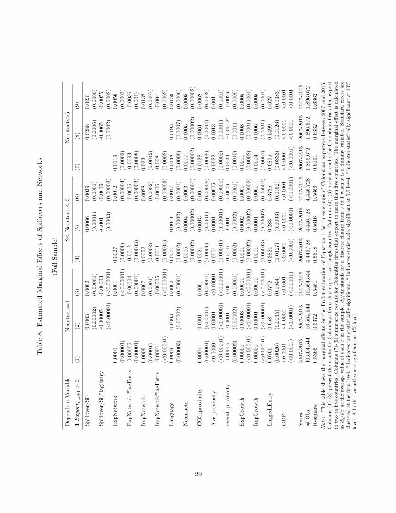
Tab

le8:

Est

imat

edM

argi

nal

Eff

ects

ofS

pil

love

rsan

dN

etw

orks

(Fu

llS

am

ple

)

Dep

enden

tV

aria

ble

:N

conta

cts=

12≤

Nco

nta

cts≤

5N

conta

cts>

5

1[Export i,c,t+1>

0](1

)(2

)(3

)(4

)(5

)(6

)(7

)(8

)(9

)

Spillo

ver/

SE

0.00

030.

0002

0.00

660.

0039

0.02

880.

0231

(0.0

0002

)(0

.000

01)

(0.0

001)

(0.0

001)

(0.0

006)

(0.0

006)

Spillo

ver/

SE

*lag

Entr

y-0

.000

05-0

.000

03-0

.001

-0.0

006

-0.0

065

-0.0

055

(<0.

0000

1)(<

0.00

001)

(0.0

003)

(0.0

0003

)(0

.000

2)(0

.000

2)E

xpN

etw

ork

0.00

010.

0001

0.00

270.

0012

0.01

190.

0056

(0.0

0001

)(<

0.00

001)

(0.0

001)

(0.0

0004

)(0

.000

2)(0

.000

3)E

xpN

etw

ork

*lag

Entr

y-0

.000

05-0

.000

04-0

.001

2-0

.000

6-0

.009

3-0

.003

6(0

.000

01)

(0.0

0001

)(0

.000

03)

(0.0

0003

)(0

.000

8)(0

.001

)Im

pN

etw

ork

0.00

090.

0007

0.00

520.

0028

0.03

30.

0132

(0.0

001)

(0.0

001)

(0.0

003)

(0.0

002)

(0.0

012)

(0.0

007)

ImpN

etw

ork*l

agE

ntr

y-0

.000

1-0

.000

05-0

.001

1-0

.000

6-0

.008

-0.0

04(<

0.00

001)

(<0.

0000

1)(0

.000

04)

(0.0

0003

)(0

.000

2)(0

.000

2)L

angu

age

0.00

040.

0003

0.00

020.

0071

0.00

410.

0027

0.03

480.

0193

0.01

59(0

.000

03)

(0.0

0002

)(0

.000

01)

(0.0

002)

(0.0

002)

(0.0

001)

(0.0

009)

(0.0

007)

(0.0

006)

Nco

nta

cts

0.00

050.

0004

0.00

030.

0007

0.00

050.

0005

(0.0

0002

)(0

.000

02)

(0.0

0001

)(0

.000

02)

(0.0

0002

)(0

.000

02)

CO

Lpro

xim

ity

0.00

010.

0001

0.00

010.

0021

0.00

150.

0011

0.01

280.

0061

0.00

62(0

.000

01)

(0.0

0001

)(0

.000

01)

(0.0

001)

(0.0

001)

(0.0

0005

)(0

.000

5)(0

.000

4)(0

.000

3)A

vepro

xim

ity

<0.

0000

10.

0000

1<

0.00

001

0.00

010.

0001

0.00

005

0.00

220.

0013

0.00

11(<

0.00

001)

(<0.

0000

1)(<

0.00

001)

(0.0

0001

)(0

.000

01)

(0.0

0001

)(0

.000

2)(0

.000

1)(0

.000

1)ov

eral

lpro

xim

ity

-0.0

0005

-0.0

001

-0.0

001

-0.0

007

-0.0

01-0

.000

90.

0034

−0.

0012

a-0

.002

9(0

.000

02)

(0.0

0002

)(0

.000

01)

(0.0

002)

(0.0

002)

(0.0

001)

(0.0

015)

(0.0

01)

(0.0

009)

ExpG

row

th0.

0000

10.

0000

30.

0000

10.

0001

0.00

020.

0001

0.00

110.

0008

0.00

05(<

0.00

001)

(<0.

0000

1)(<

0.00

001)

(0.0

0002

)(0

.000

02)

(0.0

0002

)(0

.000

2)(0

.000

1)(0

.000

1)Im

pG

row

th0.

0000

10.

0000

10.

0000

10.

0001

0.00

010.

0001

0.00

040.

0006

0.00

05(<

0.00

001)

(<0.

0000

1)(<

0.00

001)

(0.0

0003

)(0

.000

02)

(0.0

0002

)(0

.000

2)(0

.000

1)(0

.000

1)L

agge

dE

ntr

y0.

0765

0.05

80.

0772

0.38

210.

283

0.37

250.

6895

0.54

990.

627

(0.0

026)

(0.0

035)

(0.0

044)

(0.0

127)

(0.0

093)

(0.0

152)

(0.0

333)

(0.0

126)

(0.0

383)

GD

P<

0.00

01<

0.00

01<

0.00

01<

0.00

01<

0.00

01<

0.00

01<

0.00

01<

0.00

01<

0.00

01(<

0.00

01)

(<0.

0001

)(<

0.00

01)

(<0.

0001

)(<

0.00

01)

(<0.

0001

)(<

0.00

01)

<0.

0001

<0.

0001

Yea

rs20

07-2

015

2007

-201

520

07-2

015

2007

-201

520

07-2

015

2007

-201

520

07-2

015

2007

-201

520

07-2

015

#O

bs.

10,5

64,5

4410

,564

,544

10,5

64,5

444,

446,

728

4,44

6,72

84,

446,

728

1,89

6,67

21,

896,

672

1,89

6,67

2R

-squar

e0.

5365

0.53

720.

5461

0.55

180.

5616

0.56

660.

6191

0.63

320.

6362

Notes:

Th

ista

ble

show

sth

em

argin

aleff

ects

for

the

Pro

bit

esti

mat

ion

of

Equ

ati

on1

for

thre

egro

up

sof

Col

omb

ian

exp

orte

rsb

etw

een

2007

and

2015

.C

olu

mn

s(1

)–(3

)p

rese

nt

the

resu

lts

for

Col

omb

ian

firm

sth

at

exp

ort

toa

sin

gle

cou

ntr

y.C

olu

mn

s(4

)–(6

)p

rese

nt

resu

lts

for

Col

omb

ian

firm

sth

atex

port

totw

oto

five

cou

ntr

ies.

Col

um

ns

(7)-

(9)

sum

mar

ize

resu

lts

for

Col

omb

ian

firm

sth

at

exp

ort

tom

ore

than

five

cou

ntr

ies.

Th

em

arg

inal

effec

tis

calc

ula

ted

asdy/dx

atth

eav

erag

eva

lue

of

each

xin

the

sam

ple

.dy/dx

stan

ds

for

ad

iscr

ete

chan

gefr

om0

to1

wh

enx

isa

du

mm

yva

riab

le.

Sta

nd

ard

erro

rsare

clu

ster

edat

the

firm

leve

l.a

ind

icat

esn

ot

stat

isti

cally

sign

ifica

nt.

bin

dic

ates

stati

stic

ally

sign

ifica

nt

at5%

level

.c

ind

icat

esst

atis

tica

lly

sign

ifica

nt

at10

%le

vel.

All

oth

erva

riab

les

are

sign

ifica

nt

at

1%

leve

l.

29

5 Robustness Checks

As discussed in Section 3, this paper potentially suffers from the problem of correlated unob-

servables. That is, an exporting firm entering a new market might not necessarily because it

learned about that market through information spillover or network search, but because that

market is similar to the firms’ previous export destinations or its home country. The use of

firm-to-firm measure of networks help us resolve this problem when estimating the network

effect, since network search will be attributed only to those new markets to which only firm’s

trading partners export.

However, the problem still potentially exists for the spillover/SE effect. To address this con-

cern, we modified our empirical specifications by adding an adjacency dummy variable which

controls for the similarity between the new export destination and Colombia. Following

Morales et al. (2014) and Muendler and Rauch (2018), we consider the following variables:

Languagec, Contiguityc, Continentc, and IncomeGroupc. These variables are defined as

indicators taking the value of one when country c shares a border, language or income group,

respectively, with Colombia. The effect of variable Languagec has been discussed in the

baseline estimation, thus in this section we focus on the effects of the other three dummies.

We re-estimated equation (1) and (2) using various adjacency variables. The estimation

results of Colombian export to all other countries are presented in Table 9. The estima-

tion results using the sample of Colombian firms that initially only exporting to Chile are

summarized in Table 10. Moreover, Column (1)-(4) of Table 10 presents the results using

firm-to-firm measure of export networks while Column (5)-(8) using firm-to-country measure

of networks. Including Contiguity, Continent, and IncomeGroup does not change our esti-

mation results significantly. The spillover/SE and network effects are robust both in terms

of significance and the magnitudes, suggesting that firms rely on both domestic spillover

and foreign networks when choosing a new export destination, even after controlling for the

similarities between the new export destination and Colombia.

30

Table 9: Estimated Spillover and Network Effects with Adjacnecy Variables

(Full Sample)

Dependent variable: Contiguity Continent Income GroupPr(Entryi,c,t+1 = 1) (1) (2) (3) (4)

Spillover/SE 0.0018 0.0018 0.0016 0.0018(0.0001) (0.0001) (0.0001) (0.0001)

ExpNetwork 0.0006 0.0006 0.0006 0.0006(0.00003) (0.00003) (0.00003) (0.00003)

ImpNetwork 0.0009 0.0008 0.0009 0.0009(0.0001) (0.0001) (0.0001) (0.0001)

Adjacency 0.0002 0.0002 0.0001(0.00002) (0.00001) (0.00001)

Ncontacts 0.0004 0.00004 0.00004 0.00004(<0.00001) (<0.00001) (<0.00001) (<0.00001)

COL proximity 0.0007 0.0005 0.0005 0.0006(0.00003) (0.00003) (0.00003) (0.00003)

Ave proximity 0.00002 0.00002 0.00002 0.00002(<0.00001) (<0.00001) (<0.00001) (<0.00001)

Overall proximity -0.0011 -0.0009 -0.0007 -0.0009(0.0001) (0.0001) (0.00005) (0.0001)

ExpGrowth 0.0001 0.0001 0.00005 0.00005(<0.00001) (<0.00001) (<0.00001) (<0.00001)

ImpGrowth 0.00004 0.00004 0.00003 0.00003(<0.00001) (<0.00001) (<0.00001) (<0.00001)

Lagged Entry 0.1196 0.1164 0.1161 0.1194(0.003) (0.003) (0.003) (0.003)

GDP <0.0001 <0.0001 <0.0001 <0.0001(<0.0001) (<0.0001) (<0.0001) (<0.0001)

Years 2007-2015 2007-2015 2007-2015 2007-2015# Obs. 16,907,944 16,907,944 16,907,944 16,907,944R-square 0.6352 0.6357 0.6357 0.6354

Notes: This table shows the marginal effects for the Probit estimation of Equation 1 with variousadjacency variables. The marginal effect is calculated as dy/dx at the average value of each x in thesample. dy/dx stands for a discrete change from 0 to 1 when x is a dummy variable. Sector fixedeffects are controlled. Standard errors are clustered at the firm level. All estimated marginal effectsare statistically significant at 1% level.

31

Tab

le10

:E

stim

ated

Sp

illo

ver

and

Net

wor

kE

ffec

tsw

ith

Ad

jacn

ecy

Var

iab

les

(Res

tric

ted

Sam

ple

)

Dep

enden

tV

aria

ble

:F

irm

-to-

firm

net

wor

ks

Fir

m-t

o-co

untr

ynet

wor

ks

Con

tigu

ity

Con

tinen

tIn

com

eG

roup

Con

tigu

ity

Con

tinen

tIn

com

eG

roup

Pr(Entry i

,c,t+1

=1)

(1)

(2)

(3)

(4)

(5)

(6)

(7)

(8)

Spillo

ver/

SE

0.00

2***

0.00

22**

*0.

0021

***

0.00

2***

0.00

1***

0.00

11**

*0.

001*

**0.

001*

**(0

.000

5)(0

.000

6)(0

.000

6)(0

.000

6)(0

.000

3)(0

.000

4)(0

.000

4)(0

.000

3)E

xpN

etw

ork

0.00

13*

0.00

12*

0.00

13*

0.00

13*

0.00

07**

*0.

0008

***

0.00

07**

*0.

0007

***

(0.0

007)

(0.0

007)

(0.0

007)

(0.0

007)

(0.0

002)

(0.0

002)

(0.0

002)

(0.0

002)

ImpN

etw

ork

0.00

120.

0012

0.00

120.

0012

0.00

070.

0006

0.00

070.

0007

(0.0

008)

(0.0

008)

(0.0

008)

(0.0

008)

(0.0

004)

(0.0

004)

(0.0

004)

(0.0

004)

Adja

cency

0.00

13**

-0.0

001

0.00

010.

0008

**-0

.000

040.

0000

5(0

.000

6)(0

.000

1)(0

.000

1)(0

.000

4)(0

.000

1)(0

.000

04)

CO

Lpro

xim

ity

0.00

1***

0.00

07**

*0.

001*

**0.

001*

**0.

0005

***

0.00

03**

*0.

0006

***

0.00

05**

*(0

.000

2)(0

.000

2)(0

.000

3)(0

.000

2)(0

.000

2)(0

.000

1)(0

.000

2)(0

.000

2)A

vepro

xim

ity

0.00

08**

*0.

0009

***

0.00

08**

0.00

07**

*0.

0004

**0.

0004

**0.

0004

*0.

0003

**(0

.000

3)(0

.000

3)(0

.000

4)(0

.000

3)(0

.000

2)(0

.000

2)(0

.000

2)(0

.000

2)O

vera

llpro

xim

ity

-0.0

012*

**-0

.000

7*-0

.001

3***

-0.0

011*

**-0

.000

6**

-0.0

002

-0.0

006*

**-0

.000

5**

(0.0

003)

(0.0

004)

(0.0

003)

(0.0

003)

(0.0

002)

(0.0

003)

(0.0

002)

(0.0

002)

ExpG

row

th0.

0001

0.00

010.

0001

0.00

010.

0004

0.00

040.

0004

0.00

04(0

.000

3)(0

.000

3)(0

.000

3)(0

.000

3)(0

.000

4)(0

.000

4)(0

.000

4)(0

.000

4)Im

pG

row

th0.

0001

0.00

010.

0001

0.00

010.

0001

0.00

010.

0001

0.00

01(0

.000

1)(0

.000

1)(0

.000

1)(0

.000

1)(0

.000

1)(0

.000

1)(0

.000

1)(0

.000

1)G

DP

<0.

0001

***

<0.

0001

***

<0.

0001

***

<0.

0001

***

<0.

0001

***

<0.

0001

***

<0.

0001

***

<0.

0001

***

(<0.

0001

)(<

0.00

01)

(<0.

0001

)(<

0.00

01)

(<0.

0001

)(<

0.00

01)

(<0.

0001

)(<

0.00

01)

Yea

rs20

07-2

015

2007

-201

520

07-2

015

2007

-201

520

07-2

015

2007

-201

520

07-2

015

2007

-201

5#

Obs.

105,

591

105,

591

105,

591

105,

591

105,

591

105,

591

105,

591

105,

591

R-s

quar

e0.

2783

0.28

550.

2783

0.27

880.

2899

0.29

720.

290.

2904

Notes:

Th

ista

ble

show

sth

em

argi

nal

effec

tsfo

rth

eP

rob

ites

tim

atio

nof

equ

atio

n(2

)w

ith

vari

ous

adja

cen

cyva

riab

les.

Th

em

arg

inal

effec

tis

calc

ula

ted

asdy/dx

atth

eav

erag

eva

lue

of

eachx

inth

esa

mp

le.dy/dx

stan

ds

for

ad

iscr

ete

chan

ge

from

0to

1w

hen

xis

ad

um

my

vari

able

.S

ecto

rfi

xed

effec

tsar

eco

ntr

olle

d.

Sta

nd

ard

erro

rsare

clust

ered

at

the

firm

leve

l.*

ind

icat

esst

ati

stic

ally

sign

ifica

nt

at

10%

leve

l.**

ind

icat

esst

atis

tica

lly

sign

ifica

nt

at5%

leve

l.**

*in

dic

ates

stat

isti

call

ysi

gnifi

cant

at1%

leve

l.

32

6 Conclusion

This paper explores the effects of domestic spillovers and foreign networks on an exporting

firm’s expansion into new foreign markets. While there is a large literature focusing on how

spillover and network effects impact a firm’s expansion to new foreign markets, our paper is

the first to jointly estimate the following three effects: Spillover/Sequential Entry, Consumer

Exporting Network, and Supplier Network effects. It allowed us to rank the magnitudes of

the effects and to demonstrate that omitting any of these channels in the estimation speci-

fication results in a pronounced upward bias of the remaining channels. We also show that

each of these effects has a substantial economic significance, more important than several

other factors (including proximity, import and export growth rates, language, and market

size) combined.

Additionally, by matching Colombian exporting firms and Chilean importing and exporting

firms between 2007 and 2016, we are able to construct a firm-to-firm measure of the Con-

sumer Exporting Network. We showed that the finer, firm-to-firm measures of networks is

more accurate and informative than the more widely used firm-to-country measures of net-

works.

Although this paper provides empirical evidence for the spillover and network effects in a

firm’s expansion to new foreign markets, it is still imperative to formulate a theoretical

model that substantiates these effects. Moreover, this paper only analyzes the network and

spillover effects on the extensive margin of trade (i.e., the expansion to new markets) but

remains silent on their effects on the intensive margins (i.e. how much the firm sells to each

market). A model for network and spillover effects on the intensive margin of trade would

thus also be interesting. Finally, with the increasing availability of firm-level trade data, it is

possible to check whether the results of this paper can be generalized to trade between other

countries. These questions are left for future research.

References

Aitken, B., Hanson, G. H., and Harrison, A. E. (1997). Spillovers, foreign investment, and

export behavior. Journal of International Economics, 43(1-2):103–132.

Albornoz, F., Fanelli, S., and Hallak, J. C. (2016). Survival in export markets. Journal of

International Economics, 102:262–281.

33

Albornoz, F., Pardo, H. F. C., Corcos, G., and Ornelas, E. (2012). Sequential exporting.

Journal of International Economics, 88(1):17–31.

Aleksynska, M. and Peri, G. (2014). Isolating the network effect of immigrants on trade. The

World Economy, 37(3):434–455.

Antras, P. and Costinot, A. (2011). Intermediated trade. The Quarterly Journal of Eco-

nomics, 126(3):1319–1374.

Atkin, D., khandelwal, A. K., and Osman, A. (2017). Exporting and Firm Performance: Ev-

idence from a Randomized Experiment. The Quarterly Journal of Economics, 132(2):551–

615.

Barrios, S., Gorg, H., and Strobl, E. (2003). Explaining firms’ export behaviour: R&D,

spillovers and the destination market. Oxford Bulletin of Economics and Statistics,

65(4):475–496.

Barrot, J.-N. and Sauvagnat, J. (2016). Input Specificity and the Propagation of Idiosyncratic

Shocks in Production Networks. The Quarterly Journal of Economics, 131(3):1543–1592.

Benguria, F. (2015). The matching and sorting of exporting and importing firms: Theory

and evidence. Univ. of Kentucky, Mimeo.

Bernard, A. B., Bøler, E. A., and Dhingra, S. (2018a). Firm-to-firm connections in Colombian

imports. NBER Working Paper No. 24557.

Bernard, A. B. and Jensen, J. B. (2004). Why some firms export. Review of Economics and

Statistics, 86(2):561–569.

Bernard, A. B., Jensen, J. B., Redding, S. J., and Schott, P. K. (2009). The Margins of US

Trade. American Economic Review, 99(2):487–493.

Bernard, A. B. and Moxnes, A. (2018). Networks and trade. Annual Review of Economics,

(0).

Bernard, A. B., Moxnes, A., and Saito, Y. U. (2018b). Production Networks, Geography and

Firm Performance. Working papers.

Bernard, A. B., Moxnes, A., and Ulltveit-Moe, K. H. (2014). Two-sided heterogeneity and

trade. Review of Economics and Statistics, (0).

Blum, B. S., Claro, S., and Horstmann, I. (2010). Facts and figures on intermediated trade.

American Economic Review, 100(2):419–23.

34

Blum, B. S., Claro, S., and Horstmann, I. J. (2012). Import intermediaries and trade costs:

Theory and evidence. Unpublished manuscript, Rotman School of Management, University

of Toronto.

Chaney, T. (2014). The network structure of international trade. The American Economic

Review, 104(11):3600–3634.

Chaney, T. (2016). Networks in international trade. In The Oxford Handbook of the Economics

of Networks. Oxford University Press.

Chaney, T. (2018). The Gravity Equation in International Trade: An Explanation. Journal

of Political Economy, 126(1):150–177.

Choquette, E. and Meinen, P. (2015). Export spillovers: Opening the black box. The World

Economy, 38(12):1912–1946.

Ciliberto, F. and Jakel, I. C. (2017). Superstar exporters: An empirical investigation of

strategic interactions in Danish export markets. Univ. of Virginia, Mimeo.

Clerides, S. K., Lach, S., and Tybout, J. R. (1998). Is learning by exporting important?

Micro-dynamic evidence from Colombia, Mexico, and Morocco. The Quarterly Journal of

Economics, 113(3):903–947.

Combes, P.-P., Lafourcade, M., and Mayer, T. (2005). The trade-creating effects of business

and social networks: Evidence from France. Journal of International Economics, 66(1):1–

29.

Currarini, S., Jackson, M. O., and Pin, P. (2009). An economic model of friendship: Ho-

mophily, minorities, and segregation. Econometrica, 77(4):1003–1045.

Dragusanu, R. (2014). Firm-to-firm matching along the global supply chain. Harvard Univ.,

Mimeo.

Eaton, J., Eslava, M., Jinkins, D., Krizan, C., and Tybout, J. (2014). A Search and Learning

Model of Export Dynamics. 2015 Meeting Papers 1535, Society for Economic Dynamics.

Eaton, J., Eslava, M., Krizan, C. J., Kugler, M., and Tybout, J. (2009). A search and learning

model of export dynamics. Penn State Univ., Mimeo.

Garmendia, A., Llano, C., Minondo, A., and Requena, F. (2012). Networks and the disap-

pearance of the intranational home bias. Economics Letters, 116(2):178–182.

Greaney, T. M. (2009). Measuring network effects on trade: A reexamination. Japan and the

World Economy, 21(3):219–225.

35

Greenaway, D., Sousa, N., and Wakelin, K. (2004). Do domestic firms learn to export from

multinationals? European Journal of Political Economy, 20(4):1027–1043.

Hausmann, R. and Rodrik, D. (2003). Economic development as self-discovery. Journal of

Development Economics, 72(2):603–633.

He, S. (2018). Firms’ entry into foreign markets: A network centrality analysis. Working

paper.

Iacovone, L. and Javorcik, B. S. (2010). Multi-product exporters: Product churning, uncer-

tainty and export discoveries. The Economic Journal, 120(544):481–499.

Jackson, M. O. and Zenou, Y. (2015). Games on networks. In Handbook of Game Theory

with Economic Applications, volume 4, pages 95–163. Elsevier.

Kneller, R. and Pisu, M. (2007). Industrial linkages and export spillovers from FDI. The

World Economy, 30(1):105–134.

Koenig, P. (2009). Agglomeration and the export decisions of French firms. Journal of Urban

Economics, 66(3):186–195.

Koenig, P., Mayneris, F., and Poncet, S. (2010). Local export spillovers in France. European

Economic Review, 54(4):622–641.

Lawless, M. (2009). Firm export dynamics and the geography of trade. Journal of Interna-

tional Economics, 77(2):245–254.

Lim, K. (2018). Endogenous Production Networks and the Business Cycle. Working paper.

Monarch, R. (2014). It’s not you, it’s me: Breakups in US-China trade relationships. US

Census Bureau Center for Economic Studies Paper No.14-08.

Morales, E., Sheu, G., and Zahler, A. (2014). Gravity and extended gravity: Using moment

inequalities to estimate a model of export entry. NBER Working Paper No.19916.

Muendler, M.-A. and Rauch, J. E. (2018). Do employee spinoffs learn markets from their

parents? Evidence from international trade. European Economic Review, 105(C):159–173.

Nguyen, D. X. (2012). Demand uncertainty: Exporting delays and exporting failures. Journal

of International Economics, 86(2):336–344.

Nunn, N. (2007). Relationship-specificity, incomplete contracts, and the pattern of trade.

The Quarterly Journal of Economics, 122(2):569–600.

36

Petropoulou, D. (2008). Information costs, networks and intermediation in international

trade. University of Oxford, Department of Economics, Discussion Paper 370.

Rauch, J. E. (1999). Networks versus markets in international trade. Journal of International

Economics, 48(1):7–35.

Rauch, J. E. (2001). Business and social networks in international trade. Journal of Economic

Literature, pages 1177–1203.

Rauch, J. E. and Trindade, V. (2002). Ethnic Chinese networks in international trade. Review

of Economics and Statistics, 84(1):116–130.

Rauch, J. E. and Watson, J. (2004). Network intermediaries in international trade. Journal

of Economics & Management Strategy, 13(1):69–93.

Silvente, F. R. and Gimenez, J. C. (2007). Information spillovers and the choice of export des-

tination: A multinomial Logit analysis of Spanish young SMEs. Small Business Economics,

28(1):69–86.

Tintelnot, F., Kikkawa, A. K., Mogstad, M., and Dhyne, E. (2018). Trade and Domestic

Production Networks. Working paper.

Wagner, R. and Zahler, A. (2015). New exports from emerging markets: Do followers benefit

from pioneers? Journal of Development Economics, 114:203–223.

Wei, S.-J., Wei, Z., and Xu, J. (2017). Sizing up Market Failures in Export Pioneering

Activities. NBER Working Papers 23893, National Bureau of Economic Research, Inc.

37

Appendix

A Technical notes on firm-to-firm matching

Matching Colombian exporting firms to their Chilean trade partners plays a critical role in

estimating foreign network effects in our paper. We managed to do this, as the Colombian

firm-level export data record the name and address of the foreign importing firm for each

transaction. However, the foreign firm name data are very noisy. There are instances in

which the same firm is recorded differently by using various abbreviations, extra spaces,

dashes, dots, and other special signs. To clean and match the importing firm names, we used

the following procedure:

1. We dropped all observations with the missing importing firm names.

2. We eliminated the typical prefixes, suffixes, and abbreviations (e.g., “LTDA”, “LLC”,“CO.”,

“INC”).

3. We eliminated the non alpha numeric characters (e.g., . / ; () @ &).

4. We compared the importing firm names with the standardized firm names recorded in

the Chilean imports data. If the firm names were the same, we accomplished a match.

5. There are cases where the firm names have slightly different spellings than the standard-

ized firm names. In these cases, we performed a further match by address. Specifically,

we searched the address of the standardized firm through Internet, and compared it

with the address recorded in Colombian export data. If the addresses were the same,

we matched the two firms. Otherwise we failed to match.

B Alternative Specifications: Logit and Linear Probability

Model

Table B.1 and Table B.2 present the marginal effects for the Logit estimation of equation (1)

and (2), respectively. Table B.3 and Table B.4 present the estimation results using a Linear

Probability Model (LPM). These results are quantitatively and qualitatively similar to our

baseline results using Probit model.

38

Tab

leB

.1:

Est

imat

edS

pil

love

ran

dN

etw

ork

Eff

ects

:L

ogit

Mod

el(F

ull

Sam

ple

)

Chaney

’sSp

ecifi

cati

onM

odifi

edSp

ecifi

cati

ons

(Colo

mbia

nF

irm

s)

Dep

enden

tV

aria

ble

:F

rench

firm

sC

olom

bia

nfirm

sSpillo

ver/

SE

Net

wor

kSpillo

ver

/SE

Spillo

ver/

SE

Net

work

Spillo

ver/

SE

Pr(Entry i

,c,t+1

=1)

Net

wor

kL

anguag

eL

angu

age

Net

work

Languag

e(1

)(2

)(3

)(4

)(5

)(6

)(7

)(8

)(9

)

Spillo

ver/

SE

0.00

390.

0026

0.0

029

0.0

02

(0.0

001)

(0.0

001)

(0.0

001

)(0

.000

1)

ExpN

etw

ork

0.00

170.

0008

0.0

014

0.0

007

(0.0

001)

(0.0

0003

)(0

.0000

5)(0

.000

03)

ImpN

etw

ork

0.00

180.

0008

0.0

013

0.0

007

(0.0

001)

(0.0

0004

)(0

.0001

)(0

.000

04)

Langu

age

0.0

013

0.002

60.0

01

(0.0

001)

(0.0

001)

(0.0

0004)

Nco

nta

cts

0.0

016

0.00

020.

0001

0.00

010.

0001

0.00

010.0

001

0.00

01

0.0

001

(0.0

001

)(0

.0000

1)(0

.000

01)

(<0.

0000

1)(<

0.00

001)

(<0.

0000

1)(<

0.0

0001)

(<0.0

000

1)(<

0.00

001)

CO

Lpro

xim

ity

0.13

10.

0041

0.00

280.

001

0.00

210.

0009

0.00

040.0

009

0.0

005

(0.0

007)

(0.0

002

)(0

.000

1)(0

.000

03)

(0.0

001)

(0.0

0003

)(0

.0000

2)(0

.0000

3)(0

.00002)

Ave

pro

xim

ity

0.02

810.

000

10.

0000

20.

0000

10.

0001

0.00

003

0.00

001

0.0

0005

0.0

0003

(0.0

007

)(0

.0000

1)(<

0.00

001)

(<0.

0000

1)(<

0.00

001)

(<0.

0000

1)(<

0.0

0001)

(<0.0

000

1)(<

0.00

001)

Ove

rall

pro

xim

ity

-0.0

752

-0.0

052

-0.0

035

-0.0

02-0

.002

9-0

.001

7-0

.000

2−

0.000

1a-0

.000

3(0

.003

7)(0

.000

3)(0

.000

2)(0

.000

1)(0

.000

1)(0

.000

1)(0

.000

1)(0

.000

1)(0

.0001)

ExpG

row

th0.0

028

<−

0.00

0001

a0.

0008

0.00

030.

0001

0.00

010.

000

20.

0001

0.0

001

(0.0

001

)(¡

0.000

01)

(0.0

0003

)(0

.000

01)

(0.0

0001

)(0

.000

01)

(0.0

0001

)(0

.000

01)

(0.0

0001)

ImpG

row

th0.

0033

0.0

002

-0.0

0003

0.00

002

0.00

010.

0001

0.0

000

1b

0.0

001

0.00

005

(0.0

002

)(0

.000

03)

(0.0

002)

(0.0

0001

)(0

.000

01)

(0.0

0001

)(0

.0000

1)(0

.0000

1)

(0.0

0001)

Lagg

edE

ntr

y0.

422

0.21

030.

1622

0.05

460.

1159

0.04

760.

0442

0.0

809

0.0

391

(0.0

014

)(0

.0076

)(0

.004

8)(0

.002

1)(0

.003

3)(0

.001

7)(0

.0018

)(0

.0026

)(0

.0014)

GD

P0.

009

<0.

0001

<0.

0001

<0.

0001

<0.

0001

<0.

0001

<0.0

001

<0.

0001

<0.0

001

(0.0

0004)

(<0.

0001

)(<

0.00

01)

(<0.

0001

)(<

0.00

01)

(<0.

0001

)(<

0.0

001

)(<

0.00

01)

(<0.0

001

)

Yea

rs19

86-1

992

2007

-201

520

07-2

015

2007

-201

520

07-2

015

2007

-201

5200

7-201

5200

7-201

52007-

2015

#O

bs.

20,8

57,

435

13,

441,

274

16,9

07,9

4416

,907

,944

16,9

07,9

4416

,907

,944

16,9

07,

944

16,

907

,944

16,

907,9

44

R-s

quare

0.54

99

0.58

480.

595

0.62

20.

6095

0.62

950.6

247

0.61

890.6

342

Notes:

This

table

show

sth

em

argi

nal

effec

tsfo

rth

eL

ogi

tes

tim

atio

nof

equati

on

(1).

Colu

mns

(1)

pre

sents

Thom

as

Chan

ey’s

resu

lts

wit

hF

rench

firm

s.C

olu

mns

(2)-

(9)

pre

sent

the

resu

lts

wit

hC

olom

bia

nfirm

s.T

he

marg

inal

effec

tis

calc

ula

ted

asdy/dx

atth

eav

erage

valu

eof

each

xin

the

sam

ple

.dy/dx

stands

for

adis

cret

ech

ange

from

0to

1w

hen

xis

adum

my

vari

able

.Sec

tor

fixed

effec

tsare

contr

olled

.Sta

ndard

erro

rsare

clust

ered

at

the

firm

leve

l.a

indic

ate

snot

stati

stic

ally

signifi

cant.

bin

dic

ate

sst

atis

tica

lly

sign

ifica

nt

at5%

leve

l.A

llot

her

vari

able

sare

signifi

cant

at

1%

leve

l.

39

Tab

leB

.2:

Est

imat

edS

pil

love

ran

dN

etw

ork

Eff

ects

:L

ogit

Mod

el

(Res

tric

ted

Sam

ple

)

Dep

enden

tV

aria

ble

:E

xpan

din

gan

dN

on-e

xpan

din

gF

irm

sA

llF

irm

s

Pr(Entry i

,c,t+1

=1)

(1)

(2)

(3)

(4)

(5)

(6)

(7)

(8)

Spillo

ver/

SE

0.00

31**

*0.

003*

**0.

0016

**0.

0015

***

0.00

15**

*0.

0008

**(0

.001

2)(0

.001

1)(0

.000

7)(0

.000

6)(0

.000

6)(0

.000

3)E

xpN

etw

ork

0.00

31*

0.00

2**

0.00

14**

*0.

001*

*0.

0007

**0.

0007

***

(0.0

015)

(0.0

009)

(0.0

005)

(0.0

005)

(0.0

003)

(0.0

002)

ImpN

etw

ork

0.00

110.

0008

0.00

060.

0006

0.00

050.

0003

(0.0

007)

(0.0

006)

(0.0

004)

(0.0

004)

(0.0

004)

(0.0

002)

Lan

guag

e0.

0023

***

0.00

64**

*0.

0023

***

0.00

09**

0.00

1**

0.00

31**

*0.

001*

*0.

0004

**(0

.000

8)(0

.001

7)(0

.000

8)(0

.000

4)(0

.000

4)(0

.000

8)(0

.000

4)(0

.000

2)C

OL

pro

xim

ity

0.00

12**

*0.

0021

***

0.00

12**

*0.

0008

***

0.00

05**

*0.

001*

**0.

0005

***

0.00

04**

*(0

.000

3)(0

.000

5)(0

.000

3)(0

.000

2)(0

.000

1)(0

.000

2)(0

.000

1)(0

.000

1)A

vepro

xim

ity

0.00

040.

0004

0.00

030.

0002

0.00

020.

0002

0.00

020.

0001

(0.0

004)

(0.0

005)

(0.0

004)

(0.0

003)

(0.0

002)

(0.0

002)

(0.0

002)

(0.0

001)

Ove

rall

pro

xim

ity

-0.0

024*

**-0

.002

9***

-0.0

021*

**-0

.001

3*-0

.001

1***

-0.0

014*

**-0

.001

***

-0.0

005*

(0.0

008)

(0.0

011)

(0.0

008)

(0.0

007)

(0.0

004)

(0.0

005)

(0.0

004)

(0.0

003)

ExpG

row

th0.

0014

0.00

010.

0002

0.00

080.

0005

0.00

004

0.00

003

0.00

02(0

.001

1)(0

.000

4)(0

.000

4)(0

.000

6)(0

.000

4)(0

.000

2)(0

.000

2)(0

.000

2)Im

pG

row

th0.

0001

0.00

020.

0001

0.00

010.

0001

0.00

010.

0001

0.00

004

(0.0

001)

(0.0

002)

(0.0

001)

(0.0

001)

(0.0

001)

(0.0

001)

(0.0

001)

(0.0

0005

)G

DP

<0.

0001

***

<0.

0001

***

<0.

0001

***

<0.

0001

***

<0.

0001

***

<0.

0001

***

<0.

0001

***

<0.

0001

***

(<0.

0000

1)(<

0.00

001)

(<0.

0000

1)(<

0.00

001)

(<0.

0000

1)(<

0.00

001)

(<0.

0000

1)(<

0.00

001)

Yea

rs20

07-2

015

2007

-201

520

07-2

015

2007

-201

520

07-2

015

2007

-201

520

07-2

015

2007

-201

5#

Obs.

51,6

0651

,606

51,6

0651

,606

105,

591

105,

591

105,

591

105,

591

R-s

quar

e0.

2972

0.27

670.

305

0.31

030.

2729

0.25

170.

2806

0.28

91

Notes:

Th

ista

ble

show

sth

em

arg

inal

effec

tsfo

rth

eL

ogit

esti

mat

ion

ofeq

uat

ion

(2).

Col

um

n(4

)an

d(8

)p

rese

nt

the

resu

lts

wit

hfi

rm-t

o-co

untr

yex

por

tn

etw

orks,

wh

ile

all

oth

erco

lum

ns

pre

sent

resu

lts

usi

ng

firm

-to-fi

rmn

etw

orks.

Th

em

argi

nal

effec

tis

calc

ula

ted

asdy/dx

atth

eav

erag

eva

lue

ofea

chx

inth

esa

mp

le.dy/dx

stan

ds

for

ad

iscr

ete

chan

gefr

om

0to

1w

hen

xis

ad

um

my

vari

able

.S

ecto

rfi

xed

effec

tsar

eco

ntr

olle

d.

Sta

nd

ard

erro

rsar

ecl

ust

ered

atth

efi

rmle

vel

.*

ind

icat

esst

ati

stic

ally

sign

ifica

nt

at10

%le

vel.

**in

dic

ates

stat

isti

call

ysi

gnifi

cant

at5%

leve

l.**

*in

dic

ates

stati

stic

ally

sign

ifica

nt

at1%

leve

l.

40

Tab

leB

.3:

Est

imat

edS

pil

love

ran

dN

etw

ork

Eff

ects

:L

PM

(Fu

llS

am

ple

)

Chaney

’sSp

ecifi

cati

onM

odifi

edSp

ecifi

cati

ons

(Colo

mbia

nF

irm

s)

Dep

enden

tV

aria

ble

:F

rench

firm

sC

olom

bia

nfirm

sSpillo

ver

/SE

Net

wor

kSpillo

ver/

SE

Spillo

ver/

SE

Net

wor

kSpillo

ver/

SE

Pr(Entry i

,c,t+1

=1)

Net

wor

kL

angu

age

Lan

guage

Net

work

Lan

guage

(1)

(2)

(3)

(4)

(5)

(6)

(7)

(8)

(9)

Spillo

ver/

SE

0.00

880.

008

0.0

071

0.0

066

(0.0

002)

(0.0

002)

(0.0

002

)(0

.000

2)

ExpN

etw

ork

0.00

240.

0012

0.0

017

0.00

09

(0.0

001)

(0.0

001)

(0.0

001)

(0.0

001

)Im

pN

etw

ork

0.03

350.

0323

0.0

324

0.03

17

(0.0

01)

(0.0

009)

(0.0

009)

(0.0

009

)L

anguag

e0.0

10.0

118

0.0

093

(0.0

003)

(0.0

003)

(0.0

003)

Nco

nta

cts

0.00

16

0.00

160.

002

0.00

190.

0019

0.00

180.0

02

0.001

90.

0019

(0.0

0001

)(0

.000

02)

(0.0

0002

)(0

.000

02)

(0.0

0002

)(0

.000

02)

(0.0

000

2)(0

.0000

2)

(0.0

0002

)C

OL

pro

xim

ity

0.13

10.

0298

0.03

080.

0251

0.03

010.

0253

0.0

182

0.020

80.0

189

(0.0

007)

(0.0

005)

(0.0

005)

(0.0

006)

(0.0

006)

(0.0

006)

(0.0

005)

(0.0

005

)(0

.0005)

Ave

pro

xim

ity

0.0

281

-0.0

072

-0.0

105

-0.0

107

-0.0

105

-0.0

107

-0.0

107

-0.0

105

-0.0

106

(0.0

007)

(0.0

005)

(0.0

005)

(0.0

005)

(0.0

005)

(0.0

005)

(0.0

005)

(0.0

005

)(0

.0005)

Ove

rall

pro

xim

ity

-0.0

752

-0.0

076

-0.0

059

-0.0

062

-0.0

07-0

.007

0.000

8b0.

001

4-0

.0003

(0.0

037

)(0

.000

5)(0

.000

5)(0

.000

5)(0

.000

5)(0

.000

5)(0

.000

4)(0

.000

4)(0

.0004

)E

xpG

row

th0.

0028

0.00

003

0.00

20.

0013

0.00

090.

0007

0.0

01

0.000

70.0

006

(0.0

001

)(0

.000

01)

(0.0

001)

(0.0

001)

(0.0

001)

(0.0

001)

(0.0

001)

(0.0

001

)(0

.0001)

ImpG

row

th0.

0033

0.00

120.

0005

0.00

050.

0006

0.00

060.0

005

0.00

050.0

005

(0.0

002

)(0

.000

1)(0

.000

05)

(0.0

0005

)(0

.000

05)

(0.0

0005

)(0

.000

05)

(0.0

0005

)(0

.0000

5)

Lagg

edE

ntr

y0.

422

0.6

748

0.60

360.

6016

0.60

120.

5992

0.5

999

0.598

70.5

976

(0.0

014)

(0.0

032)

(0.0

036)

(0.0

035)

(0.0

035)

(0.0

035)

(0.0

035)

(0.0

035

)(0

.0035)

GD

P0.

009

<0.

0001

<0.

0001

<0.

0001

<0.

0001

<0.

0001

<0.

000

1<

0.0

001

<0.0

001

(0.0

000

4)(<

0.00

01)

(<0.

0001

)(<

0.00

01)

(<0.

0001

)(<

0.00

01)

(<0.

0001)

(<0.

000

1)(<

0.0

001)

Yea

rs19

86-1

992

2007

-201

520

07-2

015

2007

-201

520

07-2

015

2007

-201

520

07-2

015

200

7-201

52007-

2015

#O

bs.

20,8

57,4

3513,

441

,274

16,9

07,9

4416

,907

,944

16,9

07,9

4416

,907

,944

16,9

07,

944

16,

907

,944

16,9

07,

944

R-s

quare

0.54

990.

5009

0.45

930.

4602

0.46

070.

4614

0.4

607

0.46

14

0.4

618

Notes:

This

table

show

sth

ees

tim

atio

nre

sult

sof

equat

ion

(1)

usi

ng

Lin

ear

Pro

bab

ilit

yM

odel

(LP

M).

Colu

mns

(1)

pre

sents

Thom

as

Chaney

’sre

sult

sw

ith

Fre

nch

firm

s.C

olum

ns

(2)-

(9)

pre

sent

the

resu

lts

wit

hC

olom

bia

nfirm

s.T

he

marg

inal

effec

tis

calc

ula

ted

asdy/dx

atth

eav

erage

valu

eof

each

xin

the

sam

ple

.dy/dx

stands

for

adis

cret

ech

ange

from

0to

1w

hen

xis

adum

my

vari

able

.Sec

tor

fixed

effec

tsar

eco

ntr

olle

d.

Sta

ndard

erro

rsare

clust

ered

atth

efirm

leve

l.a

indic

ate

snot

stati

stic

ally

sign

ifica

nt.

bin

dic

ates

stat

isti

cally

sign

ifica

nt

at5%

leve

l.A

llot

her

vari

able

sar

esi

gnifi

cant

at

1%

level

.

41

Tab

leB

.4:

Est

imat

edS

pil

love

ran

dN

etw

ork

Eff

ects

:L

PM

(Res

tric

ted

Sam

ple

)

Dep

enden

tV

aria

ble

:E

xpan

din

gan

dN

on-e

xpan

din

gF

irm

sA

llF

irm

s

Pr(Entry i

,c,t+1

=1)

(1)

(2)

(3)

(4)

(5)

(6)

(7)

(8)

Spillo

ver/

SE

0.00

75**

*0.

0074

***

0.00

77**

*0.

0036

***

0.00

36**

*0.

0036

***

(0.0

022)

(0.0

022)

(0.0

021)

(0.0

01)

(0.0

01)

(0.0

01)

ExpN

etw

ork

0.06

85**

*0.

0681

***

-0.0

008

0.03

65**

*0.

0365

***

0.00

02(0

.024

)(0

.023

9)(0

.000

9)(0

.011

4)(0

.011

4)(0

.000

5)Im

pN

etw

ork

0.00

90.

009

0.01

120.

008*

0.00

81*

0.00

91*

(0.0

071)

(0.0

071)

(0.0

075)

(0.0

045)

(0.0

045)

(0.0

047)

Lan

guag

e0.

0158

***

0.01

75**

*0.

0151

***

0.01

59**

*0.

0077

***

0.00

84**

*0.

0071

***

0.00

74**

*(0

.002

2)(0

.002

4)(0

.002

2)(0

.002

2)(0

.001

1)(0

.001

2)(0

.001

1)(0

.001

1)C

OL

pro

xim

ity

0.02

33**

*0.

0268

***

0.02

35**

*0.

0235

***

0.01

15**

*0.

0132

***

0.01

16**

*0.

0117

***

(0.0

038)

(0.0

038)

(0.0

038)

(0.0

038)

(0.0

019)

(0.0

019)

(0.0

019)

(0.0

019)

Ave

pro

xim

ity

-0.0

073

-0.0

117

-0.0

117

-0.0

07-0

.003

6-0

.005

4-0

.005

4-0

.003

7(0

.007

2)(0

.007

5)(0

.007

5)(0

.007

3)(0

.003

5)(0

.003

6)(0

.003

6)(0

.003

6)O

vera

llpro

xim

ity

-0.0

005*

*-0

.000

5**

-0.0

004*

-0.0

005*

*-0

.000

2*-0

.000

2*-0

.000

2-0

.000

2*(0

.000

2)(0

.000

3)(0

.000

2)(0

.000

2)(0

.000

1)(0

.000

1)(0

.000

1)(0

.000

1)E

xpG

row

th0.

0375

**0.

0014

0.00

160.

0358

**0.

0203

**0.

0011

0.00

10.

0192

**(0

.017

6)(0

.015

)(0

.015

2)(0

.016

9)(0

.01)

(0.0

089)

(0.0

089)

(0.0

097)

ImpG

row

th0.

0011

*0.

0009

0.00

090.

0011

0.00

060.

0005

0.00

050.

0005

(0.0

007)

(0.0

007)

(0.0

007)

(0.0

007)

(0.0

004)

(0.0

004)

(0.0

004)

(0.0

004)

GD

P<

0.00

01**

*<

0.00

01**

*<

0.00

01**

*<

0.00

01**

*<

0.00

01**

*<

0.00

01**

*<

0.00

01**

*<

0.00

01**

*(<

0.00

01)

(<0.

0001

)(<

0.00

01)

(<0.

0001

)(<

0.00

01)

(<0.

0001

)(<

0.00

01)

(<0.

0001

)

Yea

rs20

07-2

015

2007

-201

520

07-2

015

2007

-201

520

07-2

015

2007

-201

520

07-2

015

2007

-201

5#

Obs.

51,6

0651

,606

51,6

0651

,606

105,

591

105,

591

105,

591

105,

591

R-s

quar

e0.

0371

0.04

0.04

120.

0375

0.01

860.

0205

0.02

110.

0191

Notes:

Th

ista

ble

show

sth

ees

tim

atio

nre

sult

sof

equ

ati

on(2

)u

sin

gL

inea

rP

rob

abilit

yM

od

el(L

PM

).C

olu

mn

(4)

an

d(8

)p

rese

nt

the

resu

lts

wit

hfi

rm-t

o-co

untr

yex

port

net

wor

ks,

wh

ile

all

oth

erco

lum

ns

pre

sent

resu

lts

usi

ng

firm

-to-

firm

net

work

s.T

he

mar

gin

aleff

ect

isca

lcu

late

dasdy/dx

at

the

aver

age

valu

eof

each

xin

the

sam

ple

.dy/dx

stan

ds

for

ad

iscr

ete

chan

gefr

om0

to1

wh

enx

isa

du

mm

yva

riab

le.

Sec

tor

fixed

effec

tsar

eco

n-

trol

led

.S

tan

dard

erro

rsar

ecl

ust

ered

at

the

firm

level

.*

ind

icat

esst

atis

tica

lly

sign

ifica

nt

at10%

leve

l.**

ind

icate

sst

atis

tica

lly

sign

ifica

nt

at5%

leve

l.***

ind

icate

sst

atis

tica

lly

sign

ifica

nt

at1%

leve

l.

42

C Summary Statistics

Table C.1 and Table C.2 present the summary statistics and correlation coefficients between

variables for the sample of Colombian firms that originally export to Chile only.

D Maps for Spillover and Export Network Effects

Figure 3 shows the geographic maps for the new destinations that the Colombian firms ex-

pand to as well as the export destinations of their peer firms and their matched Chilean

trade partners. The intensity of the color represents the frequencies of exports. We can see

that there is a large overlap between the Colombian firm’s new export destinations and the

export destinations of their peer firms and Chilean trade partners, suggesting that exporting

firms may rely on both domestic spillovers and foreign networks when choosing a new export

destination.

43

Tab

leC

.1:

Su

mm

ary

Sta

tist

ics

Fir

m-t

o-firm

Fir

m-t

o-co

untr

yC

OL

Ave

Ove

rall

Entr

ySpillo

ver/

SE

ExpN

etw

ork

Exp

oNet

wor

kIm

pN

etw

ork

Lan

guag

epro

xim

ity

pro

xim

ity

pro

xim

ity

ExpG

row

thIm

pG

row

thG

DP

Mea

n0.

0022

0.17

260.

0042

0.29

580.

0129

0.09

840.

1744

0.11

330.

3347

0.0

028

0.5

471

3.3

8×

101

0

Med

ian

00

00

00

0.09

90.

0841

0.26

880

125942.6

2Std

.D

ev.

0.04

730.

3779

0.0

650.

4564

0.11

260.

2978

0.20

640.

0983

0.33

550.

052

80.4

978

1.4

2×

101

1

Min

00

00

00

0.05

160.

053

0.09

760

0130.4

654

Max

11

11

11

1.36

330.

8645

3.28

441

11.8

1×

101

2

No.

ofon

es23

718

,223

448

31,3

291,

357

10,3

86295

57,7

65

Per

cent

ofon

es0.

22%

17.2

6%0.

42%

29.5

8%1.

29%

9.84

%0.

28%

54.7

1%

Tab

leC

.2:

Cor

rela

tion

Coeffi

cien

tsB

etw

een

Var

iab

les

Fir

m-t

o-firm

Fir

m-t

o-co

untr

yC

OL

Ave

Ove

rall

Entr

ySpillo

ver/

SE

ExpN

etw

ork

ExpN

etw

ork

ImpN

etw

ork

Lan

guag

epro

xim

ity

pro

xim

ity

pro

xim

ity

ExpG

row

thIm

pG

row

thG

DP

Entr

y1

Spillo

ver/

SE

0.08

271

Fir

m-t

o-firm

ExpN

etw

ork

0.06

770.

0674

1F

irm

-to-

countr

yE

xpN

etw

ork

0.06

660.

344

0.10

071

ImpN

etw

ork

0.04

430.

0583

0.09

220.

1384

1L

angu

age

0.08

450.

4086

0.12

910.

4027

0.02

671

CO

Lpro

xim

ity

0.08

50.

3898

0.07

990.

2782

-0.0

060.

5967

1A

vepro

xim

ity

0.05

190.

2676

0.14

630.

2953

0.01

410.

6203

0.43

891

Ove

rall

pro

xim

ity

-0.0

18-0

.074

3-0

.028

4-0

.122

3-0

.030

2-0

.115

-0.0

536

-0.1

203

1E

xpG

row

th0.

0354

0.04

890.

4244

0.07

930.

072

0.08

550.

0472

0.10

58-0

.021

1Im

pG

row

th0.

0021

-0.0

251

0.01

290.

009

0.00

86-0

.015

-0.0

657

-0.0

444

0.0

036

0.0

132

1G

DP

0.08

080.

2244

0.05

790.

2545

0.25

26-0

.037

9-0

.035

9-0

.033

3-0

.0861

0.0566

-0.0

037

1

44

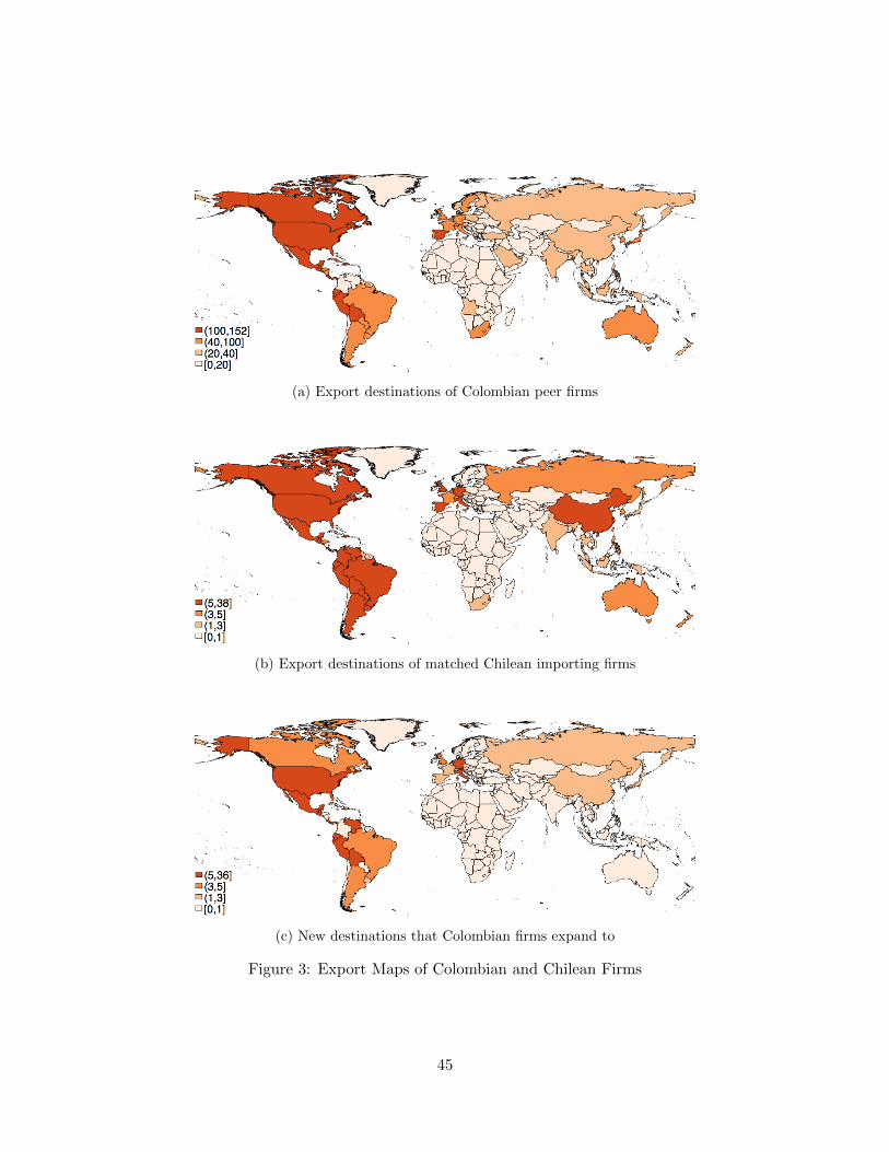
(a) Export destinations of Colombian peer firms

(b) Export destinations of matched Chilean importing firms

(c) New destinations that Colombian firms expand to

Figure 3: Export Maps of Colombian and Chilean Firms

45