Bounded Approaches in Radio Labeling Square Grids

A Thesis Presented toThe Faculty of the Mathematics Program

California State University Channel Islands

In (Partial) Fulfillmentof the Requirements for the Degree

Master of Science

Dev Ananda

May, 2015

c© 2015 Dev AnandaALL RIGHTS RESERVED

Signature page for the Masters in Mathematics Thesis of Dev AnandaAPPROVED FOR THE MATHEMATICS PROGRAM

Cynthia Wyels, Thesis Advisor Date

Jorge Garcia, Thesis Committee Date

APPROVED FOR THE UNIVERSITY

Dr. Gary A. Berg, AVP Extended University Date

For my dear parents, Kumar and Viji Ananda, whose loving encouragement andaffection have made my dreams possible throughout my life.

Acknowledgements

This dissertation would not have been written without the sagely advice and encour-agement of my senior thesis advisor, Dr. Cynthia Wyels, whose countless hours ofpatience and insight kept me focused. I graciously offer thanks to my other commit-tee advisor, Dr. Jorge Garcia, for contributing his considerable expertise. I wouldalso like to express my gratitude to Dr. Ivona Grzegorczyk and Dr. Jesse Elliott, andas well as all of the esteemed members of the California State University ChannelIslands Faculty for their generosity and direction in providing a healthy environmentwith which to undertake such an inspiring and cathartic endeavor. In addition, letme take a moment to express my profound thanks to Jacky Burneo and AmandaMarquez for taking care of all of the small things, and making all of this a little lessdaunting. Thank you to Maggy Tomova, Tian-Shun Allan Jiang, Eduardo Calles,and Henry Gomez, without whose scholarly efforts, this project would not have atall been possible. Lastly, I owe a debt of gratitude to CSUCI for renewing my thirstfor knowledge and passion for success.

v

Abstract

Bounded Approaches in Radio Labeling Square Grids

by Dev Ananda

Let d(u, v) denote the distance between two vertices u and v on a graph G and letdiam(G) denote the diameter of such a graph G. A connected graph G has a radiolabeling f if, for all vertices u, v of G,

d(u, v) + |f(u)− f(v)| ≥ diam(G) + 1. (1)

The span of the labeling function f is the maximum integer assigned by f . Theradio number of a graph G, rn(G), is the minimum possible span obtained overall possible radio labelings of the graph G. A path graph Pn has n consecutivevertices along n − 1 consecutive edges. A grid graph is defined as the Cartesianproduct of two path graphs, and a square grid graph is obtained by taking theproduct of identical path graphs Pn�Pn. In this paper, the radio number of alleven grid graphs is determined using bounding techniques alone, while establishingfundamental guidelines for odd grids and distance-maximizing labelings, in general.

vi

Table of Contents

1. Introduction . . . . . . . . . . . . . . . . . . . . . . . . . . . . . . . . . . . . . . . . . . . . . . . . . . . . . . . . . . . . . . . . . . . . . . . . . . . 1

1.1. Useful Definitions . . . . . . . . . . . . . . . . . . . . . . . . . . . . . . . . . . . . . . . . . . . . . . . . . . . . . . . . . . . . . 2

1.2. Paths . . . . . . . . . . . . . . . . . . . . . . . . . . . . . . . . . . . . . . . . . . . . . . . . . . . . . . . . . . . . . . . . . . . . . . . . . 4

1.3. Grids. . . . . . . . . . . . . . . . . . . . . . . . . . . . . . . . . . . . . . . . . . . . . . . . . . . . . . . . . . . . . . . . . . . . . . . . . . 5

1.4. Past Notable Work . . . . . . . . . . . . . . . . . . . . . . . . . . . . . . . . . . . . . . . . . . . . . . . . . . . . . . . . . . . . 6

2. An Upper Bound . . . . . . . . . . . . . . . . . . . . . . . . . . . . . . . . . . . . . . . . . . . . . . . . . . . . . . . . . . . . . . . . . . . . . . 8

2.1. Upper Bound For Odd Grids P2k+1�P2k+1 . . . . . . . . . . . . . . . . . . . . . . . . . . . . . . . . . . . . 8

2.2. Upper Bound For Even Grids P2k�P2k . . . . . . . . . . . . . . . . . . . . . . . . . . . . . . . . . . . . . . . . 13

3. A Lower Bound . . . . . . . . . . . . . . . . . . . . . . . . . . . . . . . . . . . . . . . . . . . . . . . . . . . . . . . . . . . . . . . . . . . . . . . . 25

3.1. Lower Bound For Odd Grids P2k+1�P2k+1 . . . . . . . . . . . . . . . . . . . . . . . . . . . . . . . . . . . . 27

3.2. Lower Bound For Even Grids P2k�P2k . . . . . . . . . . . . . . . . . . . . . . . . . . . . . . . . . . . . . . . . 29

4. The “Bump”. . . . . . . . . . . . . . . . . . . . . . . . . . . . . . . . . . . . . . . . . . . . . . . . . . . . . . . . . . . . . . . . . . . . . . . . . . . 31

5. Observations and Future Research . . . . . . . . . . . . . . . . . . . . . . . . . . . . . . . . . . . . . . . . . . . . . . . . . . . . . 37

References . . . . . . . . . . . . . . . . . . . . . . . . . . . . . . . . . . . . . . . . . . . . . . . . . . . . . . . . . . . . . . . . . . . . . . . . . . . . . . . . . 38

vii

1. Introduction

This paper investigates methods of determining the radio number for certain graphs and grids.We discuss the radio condition and the way in which the structure of an abstract graph affectscertain integer-valued properties of the graph. For example, the diameter of a graph or itsinter-connectivity may fundamentally affect the radio condition for non-adjacent ornon-consecutively ordered vertices. Ultimately, determining the radio number of any family ofgraphs requires consideration of its subtle nuances. In this paper, we establish upper and lowerbounds for the radio number of square grids in Sections 2 and 3 and close the gap between boundsin Section 4, The Bump, in order to determine the radio number.

In Section 2, An Upper Bound, we establish a maximum span for an optimal radio labeling.The upper bound is constructed by creating a labeling for the grid which provides a schematic bywhich the radio condition can govern. The ordering and labeling of the grid is structured such thatdistances between pairs of consecutively labeled vertices are maximized and an upper boundemerges from satisfying the various constraints. We explore the nature of constructing bounds byconstructing labelings and consider how optimal radio labelings figure into the scope of integermappings and graph space. We also review T-S. A. Jiang’s proof of the radio number of all gridsand suggest insights about the significance of graph structure within the realm of algebraicoptimization.

Section 3, A Lower Bound provides an account of distance maximization, as well as theapplication of labeling techniques in analyzing graphs. The lower bound is created by exploring thenatural characteristics of grids and examining how those characteristics can be pulled apart andtied back together to illustrate the overall coherence of grids and other graphs. By establishing alower bound, we bridge a natural “gap” between the mathematical ideal of a continuous spectrumof vertices and rigorous physical constraints that give graphs formal structure.

In Section 4, The Bump, we close the gap between the lower and upper bounds of odd andeven grids. If the lower bound admits sufficient incrementation, then the radio number of squaregrids can be determined to be the upper bound. By accounting for all pairs of vertices within thefundamental structure of the grid, the radio number is determined by showing that the span of anyviable radio labeling must be “bumped up” to the level of the upper bound and a distortion inspan arises from the intricate balance between algebraic constraint and physical order. Finally, theradio number of all even grids rn(P2k�P2k) is determined by bounded approaches, while other keyrevelations are made regarding bounding techniques and their efficacy in radio labeling and graphstructure analysis.

1

1.1. Useful Definitions.

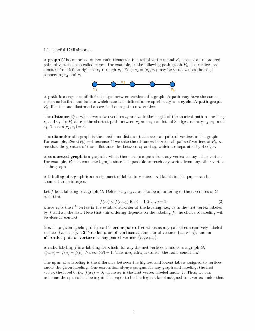
A graph G is comprised of two main elements: V, a set of vertices, and E, a set of an unorderedpairs of vertices, also called edges. For example, in the following path graph P5, the vertices aredenoted from left to right as v1 through v5. Edge e2 = (v2, v3) may be visualized as the edgeconnecting v2 and v3.

A path is a sequence of distinct edges between vertices of a graph. A path may have the samevertex as its first and last, in which case it is defined more specifically as a cycle. A path graphPn, like the one illustrated above, is then a path on n vertices.

The distance d(vi, vj) between two vertices vi and vj is the length of the shortest path connectingvi and vj . In P5 above, the shortest path between v2 and v5 consists of 3 edges, namely e2, e3, ande4. Thus, d(v2, v5) = 3.

The diameter of a graph is the maximum distance taken over all pairs of vertices in the graph.For example, diam(P5) = 4 because, if we take the distances between all pairs of vertices of P5, wesee that the greatest of those distances lies between v1 and v5, which are separated by 4 edges.

A connected graph is a graph in which there exists a path from any vertex to any other vertex.For example, P5 is a connected graph since it is possible to reach any vertex from any other vertexof the graph.

A labeling of a graph is an assignment of labels to vertices. All labels in this paper can beassumed to be integers.

Let f be a labeling of a graph G. Define {x1, x2, ..., xn} to be an ordering of the n vertices of Gsuch that

f(xi) < f(xi+1) for i = 1, 2, ..., n− 1. (2)

where xi is the ith vertex in the established order of the labeling, i.e., x1 is the first vertex labeledby f and xn the last. Note that this ordering depends on the labeling f ; the choice of labeling willbe clear in context.

Now, in a given labeling, define a 1st-order pair of vertices as any pair of consecutively labeledvertices {xi, xi+1}, a 2nd-order pair of vertices as any pair of vertices {xi, xi+2}, and annth-order pair of vertices as any pair of vertices {xi, xi+n}.

A radio labeling f is a labeling for which, for any distinct vertices u and v in a graph G,d(u, v) + |f(u)− f(v)| ≥ diam(G) + 1. This inequality is called “the radio condition.”

The span of a labeling is the difference between the highest and lowest labels assigned to verticesunder the given labeling. Our convention always assigns, for any graph and labeling, the firstvertex the label 0, i.e. f(x1) = 0, where x1 is the first vertex labeled under f . Thus, we canre-define the span of a labeling in this paper to be the highest label assigned to a vertex under that

2

graph labeling. If a graph G with labeling f has an ordering {x1, x2, ..., xn} of verticescorresponding to (2), then span(f) = f(xn).

The radio number of a graph G, rn(G), is then the minimum possible span across all radiolabelings of G. In other words, if all radio labelings of a graph are considered, then the radionumber is the lowest span for that graph under any of those radio labelings.

3

1.2. Paths.

A path graph Pn is a connected set of n vertices connected by n− 1 edges, in which theterminal vertices have degree 1 and all others degree two. Below are examples of path graphs P1,P2, and P4.

Figure 1. [top to bottom: Path graphs P1, P2 and P4]

Figure 2 illustrates radio labelings f1 and f2, respectively, of P4. Note that the radiolabeling f2 of P4 is non-optimal – that is, span(f2) > rn(P4). Radio labeling f1, however, isoptimal – that is, span(f1) = rn(P4), as discussed later in Section 1.4.

Figure 2. Radio labelings of P4

[ top: radio labeling f1; bottom: optimal radio labeling f2 ]

4

1.3. Grids.

A grid graph is the Cartesian product of two path graphs. The grids that are addressed inthis paper are composed of two identical paths that construct a square grid graph. So, henceforth,for this paper, a grid will refer to a square grid, Pn�Pn. An odd grid P2k+1�P2k+1 is constructedfrom odd paths, and an even grid P2k�P2k from even paths. Odd grid P3�P3 is depicted below,first, as a set of vertices and edges, and subsequently, as a set of vertices in an array of boxes. Inthe latter case, the boxes represent vertices, and two vertices are considered adjacent if they sharean edge.

Figure 3. A grid as a set of labeled boxes denoting vertices

An optimal radio labeling for G = P3�P3 is illustrated below. Note that the highest vertexlabel represents the radio number. In this case, we see that diam(G) = 4. Thus, for this graph,any radio labeling f must satisfy the following inequality: d(u, v) + |f(u)− f(v)| ≥ 4 + 1 = 5 for alldistinct vertices u and v. In the radio labeling f∗ below, v4 is the last vertex in the ordering andf∗(v4) = 17. Thus, span(f∗) = 17 (as denoted in blue). Since there is no radio labeling ofP3�P3 that produces a lower span, rn(P3���P3) = 17.

Figure 4. A radio labeling of 3x3 grid P3�P3

5

1.4. Past Notable Work.

Radio labeling is a realm of graph theory motivated by a problem faced in the FCC’sregulation of FM radio frequencies. Radio stations are categorized into station classes. Stations areassigned channels based on certain factors. These factors include antenna height and signal power.In addition, the distances between stations also affect what channel is assigned to a radio station ofa given station class. Radio stations assigned the same channel, for example, must be a minimumdistance apart in order to satisfy FCC regulations. Similarly, stations of different channels must besome smaller distance apart. In general, stations that are in closer proximity to one another mustbe channels that are farther apart, after considering station class. This is called the channelassignment problem. Graph theory has been used to address the channel assignment problem forseveral decades. More specifically, radio labeling is the realm of graph theory that abstracts thisproblem, and its solution is thus aptly termed the radio number.

In [2], Chartrand, Erwin, and Zhang determined some bounds for the radio number of cyclegraphs Cn, as well as the radio numbers of C6, C7, and C8 in Radio Labelings of Graphs. They alsodetermined a number of key results for abstract families of graphs, in general. One of these is theassertion that, for n ≥ 6, a radio labeling of Cn cannot contain 3 consecutive labels from{1, 2, ..., n}. This result was particularly notable as it was the first to establish concrete features ofany three consecutive vertices in a radio labeling. In Section 4, The Bump, we show that, for threeconsecutively labeled vertices in a grid, a radio labeling must abide by certain restrictions.

In [3], A Graph Labeling Problem Suggested by FM Channel Restrictions, Chartrand, Erwin,and Zhang provided key results with respect to the radio labeling of graphs. They found an upperbound for the radio number of all path graphs, rn(Pn). In addition, they prove that rn(P5) = 11.These findings, described below, contribute inspiration to a considerable portion of the work in thispaper. First, they showed how to systematically eliminate possibilities among labels for anabstract graph, but even more importantly, how to develop and refine strategies that efficientlymodel the growth of integer label values in optimized labelings of large abstract graphs.

rn(Pn) ≤

{(n−12

)+ n

2 + 1, if n is even(n2

)+ 1, if n is odd

In [5], Multilevel Distance Labelings for Paths and Cycles, Liu and Zhu determined the radionumber of all paths and all cycles (cycles not shown):

rn(Pn) =

{2n2 + 2, if n is even

2n(n− 1) + 1, if n is odd.

The aforementioned result in [5] was a breakthrough finding in radio labeling. While theradio number of numerous families of graphs had been discovered, Liu and Zhu’s approach wasnovel and has importance in the scope of this paper. They presented and proved sufficientconditions for a distance labeling. The radio number is then related back as the minimum spanassociated with a distance labeling.

After providing a labeling for each of P2k and P2k+1, Liu and Zhu identified an upper boundfor the radio number of all path graphs. By analyzing distance labeling, they constructed a lowerbound for all path graphs. The key feature in their work was the use of a distance-maximizingstrategy. Later in this paper, we will see that minimum spans result from maximizing the sum ofdistances between consecutively labeled pairs of vertices. Also, while distances are maximized,certain distance values disappear depending on the ordering chosen. Upon proving that only

6

certain orderings resulted in a distance labeling, Liu and Zhu determined rn(Pn). The relevance ofLiu and Zhu’s work to this paper is then two-fold: the conclusions (1) that a distance-maximizationstrategy used is efficient and of tremendous value for graphs of large order, such as grids, and (2)that the unique structure of specific kinds of graphs may exhibit characteristics, such as a “bump”value which excludes some distance labelings from being radio labelings.

In 2009, Calles and Gomez described the general approach for constructing upper and lowerbounds for grids. Their efforts resonate here in terms of the basic approach in determining a viablelower bound, as well as the methodology used for computing an upper bound. By analyzing thesum of all distances and arranging ordered vertices to maximize the distances between pairs ofconsecutive vertices, Calles and Gomez minimized the span of any such graph, thus determiningthe lower bound for all grids. By using their own labeling, they constructed an upper bound thatgives rise to the necessary “bump” value that closes the gap. Below, their findings are stated foreven and odd grids, respectively:

n3 − n2 − 2n+ 4 ≤ rn(P2k�P2k) ≤ n3 − n2 + 1

n3 − n2 − n+ 1 ≤ rn(P2k+1�P2k+1) ≤ n3 − n2 − n−12 + 1

Here, we extend the work of Calles and Gomez with regards to the lower bound by alsoexamining sets and arrangements of vertices in the distance-maximizing summation by consideringlost label values, the labels associated with vertices ordered first or last in the summation ofdistances between consecutive pairs of vertices and construct a more accurate lower bound for bothodd and even grids.

In terms of distance-maximization in the labelings of similar graphs and Cartesian products,Wyels and Tomova prove, in The Radio Numbers of All Graphs of Order n and Diameter n− 2,the radio number of spires. Spires are variations on path graphs. They are composed of a path anda steeple, an edge that branches off from a non-terminal vertex. The account ofdistance-maximization over the scope of Cartesian products relates a valuable result in interpretingother graphs that have unifying features like long series of connected edges or a spine thatdisconnects easily. In doing so, they characterize graphs whose diameter relate so closely to orderand provide a strong basis by which investigators can link distances and spacing to the innatestructure of connected graphs with unique components. A similar account is provided in TheRadio Number of Gear Graphs, in which radio labeling techniques applied to wheel graphs areabstracted to gear graphs, a natural extension of wheel graphs. As in our account of grids, specificlabelings are eliminated from contention based on the validity of index values under the radiocondition. Ultimately, we see that an upper bound can be determined when a lowest possible spancoincides with the exhaustive maintenance of some set of algebraic constraints.

The examples cited in this section define key methodologies in investigating various familiesof graphs, as well as abstract graphs, in general. The novelty of these prior approaches emergesthroughout the course of this investigation of grids and, as a whole, helps formulate the thoughtprocess and mathematical intuitions that succeed here.

7

2. An Upper Bound

In [2], Chartrand, Erwin, and Zhang analyze the radio condition (1) for paths and cycles.By considering the radio condition, we establish an upper bound by seeking to minimize sums ofdistances between consecutively labeled pairs of vertices. Then, the span of any such labeling isreally just an upper bound for the radio number of that graph. In section 2.1, we discuss thegeneral approach for constructing the upper bound for the radio number of odd grids P2k+1�P2k+1

and determine an upper bound in Theorem 2.1.We extend the discussion into the realms of even grids, in which the work of T-S. A. Jiang

[4] and Calles and Gomez [1] is analyzed. In section 2.2, Jiang’s labeling is defined and the labelingitself analyzed. We see that, while Jiang’s labeling does satisfy the radio condition for all pairs ofconsecutively labeled vertices, it fails to maintain (1) for what is defined here as 2nd-order pairs ofvertices. In section 2.3, we describe the methodology of Calles and Gomez and construct theirupper bound for the radio number of even grids, which is formalized here as Theorem 2.2.

2.1. Upper Bound For Odd Grids P2k+1�P2k+1.

Here, we define an ordering and construct labeling f as defined by Calles and Gomez in [1].After proving that f is a radio labeling, we calculate its span and determine and upper bound forthe radio number of all odd grids. The formalized proof is supplied below.

Theorem 2.1 (The Upper Bound for the Radio Number of Odd Grids).

rn(P2k+1�P2k+1) ≤ 8k3 + 8k2 + k.

Proof. Let G = P2k+1�P2k+1. We can substitute the diameter diam(G) = 4k into (1) and rewrite

the inequality to reflect the sum of label differences and distances between consecutively labeled

vertices:

d(xi, xi+1) + |f(xi)− f(xi+1)| ≥ 4k + 1. (3)

Note that the inequality does not necessarily satisfy the conditions of a radio labeling since only

consecutively labeled vertices are considered. First, we outline a “diagonal method” for ordering

vertices of P2k+1�P2k+1. The ordering proceeds in a cyclical diamond-like pattern a la Figure 5.

Each successive cycle of the labeling occurs just once and augments the diamond from the center

outwards, while also ordering the corner vertices in a diagonal pattern. The inner diamond and

outer diamond proceed through several cycles until they meet each other within the grid. Thus,

the labeling function f described above will be presented here as a series of labeling cycles that are

organized in Table 1.

Initial Cycle 0 (1 vertex): vk+1,k+1

The first vertex in the labeling order is assigned: it is always the center vertex of the graph.

Cycle 1: (8 vertices): v1,2k+1, vk+2,k+1, v1,1, vk+1,k+2, v2k+1,1, vk,k+1, v2k+1,2k+1, vk+1,k

The pattern enumerated above, in terms of alternately labeling vertices in a center diamond

while labeling vertices towards the outer corners, continues into the remaining cycles of the

ordering.

8

Figure 5. our labeling schematic for odd grids

Cycle 1 contains 8 distinct parts, with one vertex labeled during each part. For Cycles 2

through j, the labeling continues in these 8 distinct parts with the number of vertices labeled

within each part increasing incrementally. We see that j vertices are labeled in each of the 8 parts

of labeling Cycle j. It was alluded to previously that there are two distinct patterns that emerge

during any given labeling Cycle j ≥ 2. The vertices are ordered and labeled within each of these

two patterns alternately, and thus we will refer to the alternating patterns of labeling as Stages 1

and 2. Stage 1 is the diagonal set of vertices labeled around the center of the grid and Stage 2 is

the diagonal set of vertices labeled around the corners of the grid. The labeling hops back and

forth between Stage 1 and Stage 2 in each of four diagonally opposite directions. Thus, we really

have 4 distinct subcycles that comprise each of Stage 1 and Stage 2. The 4 subcycles will be called

Cycles j1, j2, j3, and j4. Subcycle 21 is provided for the sake of clarity:

9

Cycle 2: (16 vertices):

subcycle 21: v1,2k (Stage 1), vk+2,k (Stage 2), v2,2k+1 (Stage 1), vk+3,k+1 (Stage 2)...

subcycle 24: alternating Stages 1 & 2

Figure 6. labeling cycles for P5�P5

Notice that, during Cycle 21, two vertices are labeled in each stage. The vertices labeled in

Stage 1 are diametrically opposite about the center vertex to those labeled in Stage 2 of subcycle

21. Another 3 subcycles occur within Cycle 2 at which point Cycle 3 (as well as any subcycle)

commences, if necessary. Table 1 defines the general jth labeling cycle progression on the grid.

Figure 6 illustrates Cycles 0 - 2 on P5�P5.

10

Cycle j

Subcycle stage 1 stage 2

1

v1,2k+1−(j−1) vk+2,k+1−(j−1)

v2,2k+1−(j−2) vk+3,k+1−(j−2)

......

vj,2k+1−(j−j) vk+1+j,k+1−(j−j)

2

vj,1 vk+1+(j−1),k+2

vj−1,2 vk+1+(j−2),k+3

......

v1,j vk+1+(j−j),k+1+j

3

v2k+1,j vk,k+1+(j−1)

v2k,j−1 vk−1,k+1+(j−2)

......

v2k+1−(j−1),1 v1,k+1+(j−j)

4

v2k+1−(j−1),2k+1 vk+1−(j−1),k

v2k+1−(j−2),2k vk+1−(j−2),k−1

......

v2k+1,2k+2−j vk+1−(j−j),1

Table 1. Ordering of vertices labeled during Cycle j

We should note that any grid P2k+1�P2k+1 will have a total of k cycles under this labeling.

Define xi, i = 1, 2, ..., n2, to be ith vertex labeled in this ordering. Now, let us define the labeling

itself:

f(xi) =

0 i = 1

f(xi−1) + 2k xi−1 and xi in the same cycle

f(xi−1 + 2k + 1 xi−1 in Cycle j − 1 and xi in Cycle j.

We have shown that, if the distances between consecutive vertex pairs determine their respective

label values, then we have constructed a labeling f that abides by (1) for all 1st-order pairs of

vertices. We need only show now that higher-order pairs of vertices also satisfy (1). We see that,

for all consecutively labeled pairs of vertices in an odd grid, max d(xi, xi+1) = 2k + 1 occurs for

pairs of vertices within the same cycle. Thus, we can check the lowest label differences amongst

2nd-order pairs of vertices as follows:

f(xi+1)− f(xi) ≥ 2k

f(xi+2)− f(xi+1) ≥ 2k.

Adding these inequalities gives us:

f(xi+2)− f(xi) ≥ 4k.

11

Considering that, for all pairs of distinct vertices u and v, d(u, v) ≥ 1,

|f(xi+2)− f(xi)|+ d(xi+2, xi) ≥ 4k + 1

Thus, (1) is satisfied for all 2nd-order pairs of vertices in the grid. As

f(xi+3)− f(xi) > f(xi+2)− f(xi), we have confirmed that radio condition (1) is satisfied for

3rd-order pairs of vertices, and thus all distinct pairs of vertices in the grid. Therefore, f must be a

radio labeling. Below, we formulate the span of the labeling by considering labeling differences

between consecutively labeled vertices both within cycles and between cycles.

The distance between each pair of consecutive vertices within Cycle j is 2k + 1. For all

cycles j = 2, 3, ..., k, the distance between the first vertex in Cycle j and the final vertex labeled in

Cycle j − 1 is 2k. The distance between each pair of consecutive vertices within Cycle j is 2k + 1.

Now, we ascertain the value added to the span due to these two unique kinds of pairs of

consecutively labeled vertices under labeling f : (i) the value added to the span as result of all pairs

of consecutively labeled vertices within the same cycle and (ii) the value added to the span

associated with consecutively labeled vertices that are in different cycles. Since the diameter of an

odd grid P2k+1�P2k+1 is 4k + 1, pairs of consecutively labeled vertices that are part of different

labeling cycles must add 4k+ 1− 2k = 2k+ 1 to the overall span and pairs of consecutively labeled

vertices that are part of the same cycle add 4k + 1− (2k + 1) = 2k to the overall span. The

following table gives the calculation of the span across all the cycles of an odd grid. These cyclic

spans are summed, culminating in a span for the graph itself.

labeling schema for f

Cycle # # of vertices to label value added to span(f)

0 1 0

1 8 2k + 1 + (8− 1)(2k)

2 16 2k + 1 + (16− 1)(2k)

3 24 2k + 1 + (24− 1)(2k)

k 8k 2k + 1 + (8k − 1)(2k)

Table 2. How vertices labeled in Cycle k add to span

The span is computed by summing all the label differences between consecutive vertex pairs. Since

there are a total of j = k cycles, we have 8k − 1 pairs of vertices within the same cycle that add a

total of 2k(8k − 1) to span(f) and j = k pairs of vertices in different (but consecutive) cycles that

add k(2k + 1) to span(f). The span is thus:

span(f) = f(x(2k+1)2) ≥k∑j=1

[2k + 1 + 2k(8j − 1))] (4)

We find an aggregate span by considering label sums as a consequence of each cycle and its

structure. Multiplying out and simplifying (4) yields

f(x(2k+1)2) =

k∑j=1

[2k(8j) + 1] = k +

k∑j=1

2k(8j)

12

= k + 16k

k∑j=1

j

Using a summation formula to replace our sigma notation, we get

f(x(2k+1)2) = k + 16k

[k(k + 1)

2

]f(x(2k+1)2) = k + 8k3 + 8k2

f(x(2k+1)2 = 8k3 + 8k2 + k. (5)

Since f is a radio labeling and f(x1) = 0, (5) constitutes an upper bound for the radio number of

P2k+1�P2k+1. As a result, the span of f is really just the upper bound:

rn(P2k+1�P2k+1) ≤ 8k3 + 8k2 + k. (6)

�

2.2. Upper Bound For Even Grids P2k�P2k.

In The Radio Number of Grid Graphs [4], Jiang both comprehensively describes a labelingwhose span is the radio number of square grids as well as determines the radio number of all grids.In Section 2.2, we both define the labeling mathematically and disprove Jiang’s radio number foreven grids. However, we see that Jiang’s labeling can be used to generate the radio number of evengrids. Jiang’s methods bypass reconciling the gap between bounds by employing a trace numberanalysis of all grids. Here, we focus on the pitfalls of radio labeling techniques that fail to ensurethat the radio condition is uniformly satisfied for all possible pairs of vertices. Jiang manages toavoid failing (1) by changing the labeling rules when necessary mathematically, but does not showthis algebraically. In addition, as alluded to before, Jiang’s labeling produces a span that exceedshis radio number. We address those concerns in Section 2.2.2.

2.2.1. Jiang’s Labeling and its Span.

Theorem 2.2 (The Upper Bound for the Radio Number of Even Grids).

rn(P2k�P2k) ≤ 8k3 − 4k2 − 4k + 6.

Proof. We reconstruct the upper bound associated with Jiang’s labeling algebraically.

The ordering Jiang creates for even grids bears some resemblance to the labeling we use for

odd ones. We maximize distances by ensuring that consecutively labeled vertices are on opposite

sides of the grid. To ensure that computation of the associated span is organized and accurate, we

distinguish between labeling two halves of the grid. Define Phase 1 as the ordering for the

bottom-left and top-right quadrants, and Phase 2 as the equivalent for the top-left and

bottom-right quadrants.

13

Figure 7. Jiang’s Ordering [4]

The Phase 1 ordering is comprised of 2k− 2 cycles, as depicted in Figure 7. In Cycle 1, the first 4

vertices are ordered.

Cycle 1 (4 vertices):

vk,k+1, v2k,1, v1,2k, vk+1,k

Each stage after Cycle 1 consists of 2 stages, or subcycles, that take place in quadrants

opposite to one another. We see that these labeling cycles continue by hopping between diagonal

quadrants and labeling corresponding vertices in each respective quadrant within Stages 1 and 2.

Cycle 2 orders vertices in the diagonals adjacent to vertices labeled in the previous cycle.

Generally, the cycles label the vertices along diagonals within each of the diagonal quadrants while

spanning out to cover the rest of the vertices in those quadrants. This labeling of the grid also

features a snake-like progression between cycles that preserves diagonalized ordering. It is of use

also to recognize that Cycle k orders vertices in the center diagonals of each of the quadrants as we

will build our computation of the upper bound around this cycle. We outline the labeling of the

vertices during each cycle below (stage in parentheses):

Cycle 2: (4 vertices)

v2,2k (Stage 1), vk+2,k (Stage 2), v1,2k−1 (1), vk+1,k−1 (2)

Cycle 3: (6 vertices)

v1,2k−2 (1), vk+1,k−2 (2), v2,2k−1 (1), vk+2,k−1 (2), v3,2k (1), vk+3,k (2)...

14

Cycle k − 1: (2k − 2 vertices)

vk−1,2k (1), v2k−1,k (2), vk−2,2k−1 (1), v2k−2,k−1 (2), ... , v1,k+2 (1), vk,2 (2)

Cycle k: (2k vertices)

v1,k+1 (1), vk+1,1 (2), v2,k+2 (1), vk+2,2 (2), ... , vk,2k (1), v2k,k (2)

Cycle k + 1: (2k − 2 vertices)

vk,2k−1 (1), v2k,k−1 (2), vk−1,2k−2 (1), v2k−1,k−2 (2), ... , v2,k+1 (1), vk+2,1 (2)...

Cycle 2k − 2: (4 vertices)

vk,k+2 (Stage 1), v2k,2 (Stage 2), vk−1,k+1 (1), v2k−1,1 (2)

Cycle j

Subcycle stage 1 stage 2

1

v1,2k+1−(j−1) vk+2,k+1−(j−1)

v2,2k+1−(j−2) vk+3,k+1−(j−2)

......

vj,2k+1−(j−j) vk+1+j,k+1−(j−j)

2

vj,1 vk+1+(j−1),k+2

vj−1,2 vk+1+(j−2),k+3

......

v1,j vk+1+(j−j),k+1+j

3

v2k+1,j vk,k+1+(j−1)

v2k,j−1) vk−1,k+1+(j−2)

......

v2k+1−(j−1),1 v1,k+1+(j−j)

4

v2k+1−(j−1),2k+1 vk+1−(j−1),k

v2k+1−(j−2),2k vk+1−(j−2),k−1

......

v2k+1,2k+2−j vk+1−(j−j),1

Table 3. Ordering of vertices labeled during Cycle j

Phase 1 concludes with the ordering of vertex v2k−1,1. Once the bottom-left and the top-right

quadrants have been ordered, ordering begins on the other pair of diagonal quadrants. Within

Phase 2, we will again refer to cycles and stages as defined above. For computational ease, we will

refer to the next labeling cycle as Cycle 1, i.e. Cycle 1 of Phase 2. Cycle 1 commences with the

labeling of vertices in each of the new quadrants.

Cycle 1 (2 vertices):

vk+1,2k (Stage 1), v1,k (Stage 2)

15

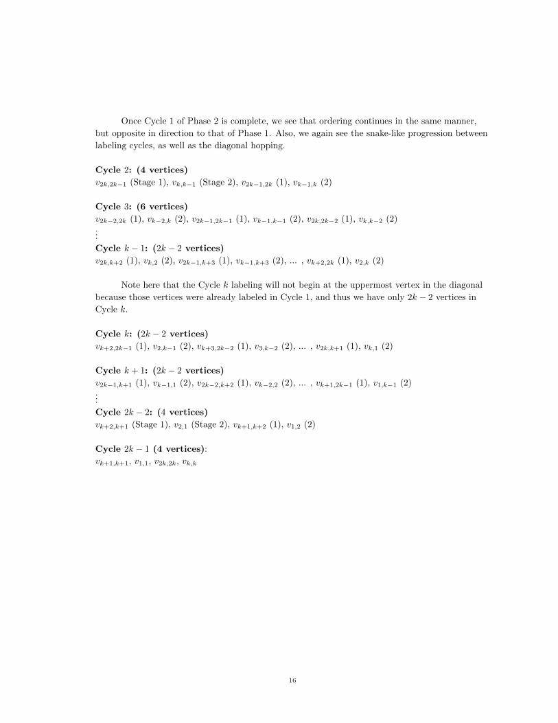
Once Cycle 1 of Phase 2 is complete, we see that ordering continues in the same manner,

but opposite in direction to that of Phase 1. Also, we again see the snake-like progression between

labeling cycles, as well as the diagonal hopping.

Cycle 2: (4 vertices)

v2k,2k−1 (Stage 1), vk,k−1 (Stage 2), v2k−1,2k (1), vk−1,k (2)

Cycle 3: (6 vertices)

v2k−2,2k (1), vk−2,k (2), v2k−1,2k−1 (1), vk−1,k−1 (2), v2k,2k−2 (1), vk,k−2 (2)...

Cycle k − 1: (2k − 2 vertices)

v2k,k+2 (1), vk,2 (2), v2k−1,k+3 (1), vk−1,k+3 (2), ... , vk+2,2k (1), v2,k (2)

Note here that the Cycle k labeling will not begin at the uppermost vertex in the diagonal

because those vertices were already labeled in Cycle 1, and thus we have only 2k − 2 vertices in

Cycle k.

Cycle k: (2k − 2 vertices)

vk+2,2k−1 (1), v2,k−1 (2), vk+3,2k−2 (1), v3,k−2 (2), ... , v2k,k+1 (1), vk,1 (2)

Cycle k + 1: (2k − 2 vertices)

v2k−1,k+1 (1), vk−1,1 (2), v2k−2,k+2 (1), vk−2,2 (2), ... , vk+1,2k−1 (1), v1,k−1 (2)...

Cycle 2k − 2: (4 vertices)

vk+2,k+1 (Stage 1), v2,1 (Stage 2), vk+1,k+2 (1), v1,2 (2)

Cycle 2k − 1 (4 vertices):

vk+1,k+1, v1,1, v2k,2k, vk,k

16

Cycle j

Subcycle stage 1 stage 2

1

v1,2k+1−(j−1) vk+2,k+1−(j−1)

v2,2k+1−(j−2) vk+3,k+1−(j−2)

......

vj,2k+1−(j−j) vk+1+j,k+1−(j−j)

2

vj,1 vk+1+(j−1),k+2

vj−1,2 vk+1+(j−2),k+3

......

v1,j vk+1+(j−j),k+1+j

3

v2k+1,j vk,k+1+(j−1)

v2k,j−1) vk−1,k+1+(j−2)

......

v2k+1−(j−1),1 v1,k+1+(j−j)

4

v2k+1−(j−1),2k+1 vk+1−(j−1),k

v2k+1−(j−2),2k vk+1−(j−2),k−1

......

v2k+1,2k+2−j vk+1−(j−j),1

Table 4. Ordering of vertices labeled during Cycle j

With the ordering of vertices established, we must ensure that our labeling is indeed a radio

labeling. We formally define Jiang’s labeling f so as to eliminate the risk of failing to satisfy the

radio condition for some pair of vertices. We make sure that the radio condition is satisfied for all

1st-order pairs of vertices by rearranging it to form our labeling function f . Therefore, define the

following for all i = 1, 2, ...4k2:

f(xi) =

0 i = 1

f(xi−1)− d(xi−1, xi) + 4k − 1 i 6= 3, 4k2 − 2

f(xi−1)− d(xi−1, xi) + 4k i = 3, 4k2 − 2

Since Jiang’s labeling f is constructed from restructuring the radio condition around pairs of

consecutive vertices, Remark 1 below will help in determining whether (1) is satisfied for all

nth-order pairs of vertices.

Remark 1. Recall that, to be a radio labeling, f must satisfy (1) for all distinct vertices of

G = P2k�P2k. Therefore, |f(u)− f(v)|+ d(u, v) ≥ diam(G) + 1, for all distinct vertices u and v of

G. More specifically, after considering the diameter, the vertices u and v satisfy (1) whenever

|f(u)− f(v)| ≥ 4k − 2.

Labeling f , as defined above, guarantees that the labeling satisfies the radio condition for all

1st-order, or consecutive, pairs of vertices. However, we must check at all steps of the labeling that

we have satisfied (1) for non-consecutive pairs as well. This is discussed in each section of the

17

computation of span(f) below. Computation is done by adding (i) the overall label value added to

the span within cycles and (ii) the overall label value added to the span between cycles (while

making the transition from one cycle to the next).

Within Cycle 1, we see that d(vk,k+1, v2k,1) = 2k, d(v2k,1, v1,2k) = 4k − 2, and

d(v1,2k, vk+1,k) = 2k. Considering the radio condition carefully and noting that

f(x1) = f(vk,k+1) = 0, we have f(x2) = 2k − 1, f(x3) = 2k − 1− (4k − 2) + 4k = 2k + 1, and

f(x4) = 4k. Therefore, the label values added to the span are 2k − 1, 2, and 2k − 1, respectively.

Summing these gives us an added span value in Cycle 1 equal to 4k. Note that normally

we always choose the lowest label value that satisfies (1) for consecutively labeled pairs of vertices,

but that our labeling makes an algebraic exception for x3. Looking carefully at the radio condition

for the first 2nd-order pair of vertices (x1, x3), we see that d(x1, x3) + |f(x1)− f(x3)| ≥ 4k − 1

under our modified labeling. Had f been defined as a “naive labeling”, f(x3) would be 1 too low

to satisfy (1). We later generalize this bump occurrence by defining a “diagonal triple” following

Proposition 1 in Section 4. It is clear that labeling f satisfies (1) for (x1, x3). We also see that

d(x2, x4) + |f(x2)− f(x4)| = 2k+ 2k− 1 ≥ 4k− 1 so (1) is also satisfied for (x2, x4) under f . After

computing the added span value associated with the rest of Phase 1 labeling, we show that f

satisfies (1) for all other nth-order pairs of vertices in Phase 1.

Within Cycles 2 through k − 1 and Cycles k + 1 through 2k − 2, we see that the

distance between each pair of consecutively labeled vertices is 2k. As a result, each pair of vertices

contributes 2k − 1 to the overall span of the grid. Each Cycle j in this part of the labeling has

2j − 1 such consecutive pairs. Since Cycles 2 through k − 1 and Cycles k + 1 through 2k − 2 are

labeled in an identical fashion, doubling the value for one of these intervals in the below

summation will suffice for both. We compute the total span value added during Cycles 2 through

k − 1 and Cycles k + 1 through 2k − 2:

{added span value} = 2 ·k−1∑j=2

(2j − 1)(2k − 1) = 2(2k − 1) ·k−1∑j=2

(2j − 1)

= (4k − 2) ·

k−1∑j=2

2j −k−1∑j=2

1

= (4k − 2) ·

2

k−1∑j=2

j − (k − 1− 1)

= (4k − 2) ·

[2

(k(k − 1)

2− 1

)− (k − 2)

]= (4k − 2) ·

[k2 − k − k

]= (4k − 2)(k2 − 2k)

= 4k3 − 10k2 + 4k. (7)

Within Cycle k, we have 2k − 1 pairs of consecutively labeled vertices. Each such pair of

consecutive vertices is distance 2k from one another. Therefore, 2k − 1 is added to the span for

each of 2k − 1 pairs. This total value added to the span is easily computed as

18

(2k − 1)2 = 4k2 − 4k + 1. It is sensible to note that this computation can very easily be added to

the above summation of label values in Cycles 2 through k − 1 and Cycles k + 1 through 2k − 2.

However, we calculate this separately for the purposes of continuity since our Phase 2 computation

of added span value in Cycle k will not contain 2k − 1 pairs, but instead 2k − 3 pairs. Thus,

[4k] + [4k3 − 10k2 + 4k] + [4k2 − 4k + 1] = 4k3 − 6k2 + 4k + 1 (8)

is associated with Phase 1 labeling within cycles.

Now, we must compute the total span value associated with Phase 1 labeling between

cycles. This is defined as the sum of span values added while labeling the first vertex in the

pending cycle after labeling the final vertex in the just-concluded cycle.

Between each of consecutive Cycles 1 through 2k − 2, we have distance 2k − 1. For

example, the last vertex labeled in Cycle 1, vk+1,k, is distance 2k − 1 from the first vertex labeled

in Cycle 2, v2,2k, and thus adds 2k to the span value of our labeling. Since there are 2k − 2− 1

such transitions between cycles, the total span value added between cycles in Phase 1 is

(2k − 3)(2k) = 4k2 − 6k.

The total span value added in Phase 1 is the sum of the overall label value added to the

span (i) within cycles and (ii) between cycles. Thus,

f(x2k2) = [4k3 − 6k2 + 4k + 1] + [4k2 − 6k]

f(x2k2) = 4k3 − 2k2 − 2k + 1. (9)

Before computing the span associated with Phase 2, we must show that f satisfies (1) for all

nth-order pairs of vertices in Phase 1. Within Cycles 2 through 2k − 2, we have either

|f(xi+2− f(xi)|+d(xi+2, xi) = 2k− 1 + 2k+ 1 or |f(xi+2− f(xi)|+d(xi+2, xi) = 2k− 1 + 2k− 1 + 2

depending on index i. In either case, |f(xi+2 − f(xi)|+ d(xi+2, xi) ≥ 4k − 1. Therefore, f satisfies

(1) for all 2nd-order pair of vertices such that i ≤ 2k2 − 2. Taking note of Remark 1, since

|f(xi+3)− f(xi)| ≥ 4k − 2 for all i in the ordering of f , all 3rd-order pairs of vertices, and thus, all

nth-order pairs of vertices within Phase 1 labeling also satisfy (1). We will confirm the same for

Phase 2 labeling before computing a final span for the grid.

Below, we outline the computation of the span of Phase 2 along with the summing of spans

for Phases 1 and 2 to produce the upper bound. It should be noted that Phase 2 contains 2k − 1

cycles as a result of the brief labeling cycle that commences Phase 2. Thus, it is also necessary to

compute span values associated with Cycle 2k − 1 as well when considering the total span value

arising from Phase 2. Lastly, we will ensure that f is a radio labeling by verifying that (1) is

satisfied for all nth-order pairs of vertices in Phase 2.

Within Cycle 1, vertices vk+1,2k and v1,k are labeled. Yet, since Phase 1 concluded, we

will define our labeling of vk+1,2k as part of “between cycles” (between phases, to be more specific).

Therefore, the labeling of v1,k, which is of distance 2k from vk+1,2k, adds 2k − 1 to the span value.

19

Within Cycles 2 through k − 1 and Cycles k + 1 through 2k − 2, the labeling

proceeds in an identical fashion, at least algebraically, to that of Phase 1, so the span value added

here is the same as in Phase 1: 4k3 − 10k2 + 4k.

Within Cycle k, as alluded to before, there are 2k − 3 pairs of consecutive vertices since

labeling in Cycle 1 reduces this number by 1 in each quadrant. This is illustrated in Figure 7.

Therefore, 2k − 1 is added to the span for each of 2k − 3 pairs. The corresponding span value

added (2k − 1)(2k − 3) = 4k2 − 8k + 3.

Within Cycle 2k − 1, the final 4 vertices are labeled. As with Cycle 1 of Phase 1, the span

value added is 4k.

Thus, the total span value added from labeling within cycles during Phase 2 is:

[2k − 1] + [4k3 − 10k2 + 4k] + [4k2 − 8k + 3] + [4k] = 4k3 − 6k2 + 2k + 2.

We now find the span value added by Phase 2 is to find the value added to the span

between cycles of Phase 2.

Between Cycle 2k − 1 of Phase 1 and Cycle 1 of Phase 2,

d(v2k−1,1, v1,2k) = 2k − 1 + k − 2 = 3k − 3. The span value added is 4k − 1− (3k − 3) = k + 2.

Between Cycle 1 and Cycle 2, d(v1,k, v2k,2k−1) = 2k − 1 + k − 1 = 3k − 2. The span

value added is 4k − 1− (3k − 2) = k + 1.

Between each of consecutive Cycles 2 through 2k − 1, there is distance 2k − 1, so the

span value added is (2k − 1− 2)(2k − 1) = 4k2 − 6k.

Consequently, the total span value added between cycles in Phase 2 is

[k + 2] + [k + 1] + [4k2 − 6k] = 4k2 − 4k + 3.

Thus, the total span value added in Phase 2 is obtained by summing the individual span

values already determined: [4k3 − 6k2 + 2k + 2] + [4k2 − 4k + 3] = 4k3 − 2k2 − 2k + 5.

Before establishing a final upper bound for rn(P2k�P2k) by summing the added span values

of Phase 1 and Phase 2 labeling, we must show that f satisfies (1) for all nth-order pairs of vertices

of Phase 2. First, for the 2nd-order pair of vertices (x2k2−1, x2k2+1),

|f(x2k2+1)− f(x2k2−1|+ d(x2k2+1, x2k2−1) = 4k − 2 + 2k − 2 = 6k − 4 ≥ 4k − 1 for k > 1.

Therefore, (1) is satisfied under f for (x2k2−1, x2k2+1).

Within Cycles 1 through 2k - 2 of Phase 2 labeling, we have the following 4 cases:

(a) |f(xi+2 − f(xi)|+ d(xi+2, xi) = 2k − 1 + 2k − 1 + 2k = 6k − 2,

20

Figure 8. Jiang’s Solution [left: the ordering; right: radio labeling f ]

(b) |f(xi+2 − f(xi)|+ d(xi+2, xi) = 2k − 1 + k + 1 + k,

(c) |f(xi+2 − f(xi)|+ d(xi+2, xi) = 2k − 1 + 2k − 1 + 2

(d) |f(xi+2 − f(xi)|+ d(xi+2, xi) = 2k − 1 + 2k + 1

depending on index i. In any of the cases, |f(xi+2 − f(xi)|+ d(xi+2, xi) ≥ 4k − 1. Therefore, f

satisfies (1) for all 2nd-order pairs of vertices for 2k2 − 1 ≤ i ≤ 4k2 − 4. Finally, as with Cycle 1 of

Phase 1, looking at the last 2nd-order pairs of vertices in Cycle 2k − 1, (x4k2−3, x4k2−1) and

(x4k2−2, x4k2), we see that:

|f(x4k2−3 − f(x4k2−1)|+ d(x4k2−3, x4k2−1) = 2k − 1 + 2 + 2k − 2 ≤ 4k − 1

|f(x4k2−2 − f(x4k2)|+ d(x4k2−2, x4k2) = 2 + 2k − 1 + 2k − 2 ≤ 4k − 1.

Therefore, all 2nd-order pair of vertices in P2k�P2k satisfy (1) under f . Again considering Remark

1, and since |f(xi+3)− f(xi)| ≥ 4k− 2 for all i in the ordering of f , all 3rd-order pairs of vertices in

Phase 2 labeling, and thus, all nth-order pairs of vertices within Phase 2 labeling also satisfy (1).

Therefore, all pairs of vertices satisfy (1) under f and f must be a radio labeling.

Finally, we sum the values added in Phases 1 and 2 to establish an upper bound:

f(x4k2) = [4k3 − 2k2 − 2k + 1] + [4k3 − 2k2 − 2k + 5]

= 8k3 − 4k2 − 4k + 6.

Thus, for odd k,

rn(P2k�P2k) ≤ 8k3 − 4k2 − 4k + 6. (10)

Now, we lay out the computation of the upper bound for the radio number of P2k�P2k for

even k. As mentioned before, most all of the aspects of the labeling and computation for even k

21

remain the same, including the snake-like progression of labeling cycles. Any differences will be

mentioned in the following discussion. We begin with Phase 1 ordering, which orders the first half

of the grid. The most notable difference is the change in diagonals present in each quadrant. As a

result, the kth labeling cycle begins in the lower right hand corner working its way up rather than

moving down from the top-left corner. This can be seen in the listing of kth Cycle vertices below.

Cycle 1 (4 vertices):

vk,k+1, v2k,1, v1,2k, vk+1,k

Cycle 2: (4 vertices)

v2,2k (Stage 1), vk+2,k (Stage 2), v1,2k−1 (1), vk+1,k−1 (2)

Cycle 3: (6 vertices)

v1,2k−2 (1), vk+1,k−2 (2), v2,2k−1 (1), vk+2,k−1 (2), v3,2k (1), vk+3,k (2)...

Cycle k − 1: (2k − 2 vertices)

vk+2,2k (1), v2,k (2), vk+3,2k−1 (1), v3,k−1 (2), ... , v2k,k+2 (1), vk,2 (2)

Cycle k: (2k vertices)

vk,2k (1), v2k,k (2), vk−1,2k−1 (1), v2k−1,k−1 (2), ... , v1,k+1 (1), vk+1,1 (2)

Cycle k + 1: (2k − 2 vertices)

v2,k+1 (1), vk+2,1 (2), v3,k+2 (1), vk+3,2 (2), ... , vk,2k−1 (1), v2k,3 (2)...

Cycle 2k − 2: (4 vertices)

vk,k+2 (Stage 1), v2k,2 (Stage 2), vk−1,k+1 (1), v2k−1,1 (2)

Phase 1 for even k concludes with the ordering of v2k−1,1. Below, the ordering pattern is set

forth for Phase 2 labeling of P2k�P2k under even k.

Cycle 1 (2 vertices):

vk+1,2k (Stage 1), v1,k (Stage 2)

Cycle 2: (4 vertices)

v2k,2k−1 (Stage 1), vk,k−1 (Stage 2), v2k−1,2k (1), vk−1,k (2)

Cycle 3: (6 vertices)

v2k−2,2k (1), vk−2,k (2), v2k−1,2k−1 (1), vk−1,k−1 (2), v2k,2k−2 (1), vk,k−2 (2)...

Cycle k − 1: (2k − 2 vertices)

vk+2,2k (1), v2,k (2), vk+3,2k−1 (1), v3,k−1 (2), ... , v2k,k+2 (1), v2,k (2)

22

Cycle k: (2k − 2 vertices)

v2k,k+1 (1), vk,1 (2), v2k−1,k+2 (1), vk−1,2 (2), ... , vk+2,2k−1 (1), v2,k−1 (2)

Cycle k + 1: (2k − 2 vertices)

vk+1,2k−1 (1), v1,k−1 (2), vk+2,2k−2 (1), v2,k−2 (2), ... , v2k−1,k+1 (1), vk−1,1 (2)...

Cycle 2k − 2: (4 vertices)

vk+2,k+1 (Stage 1), v2,1 (Stage 2), vk+1,k+2 (1), v1,2 (2)

Cycle 2k − 1 (4 vertices):

vk+1,k+1, v1,1, v2k,2k, vk,k

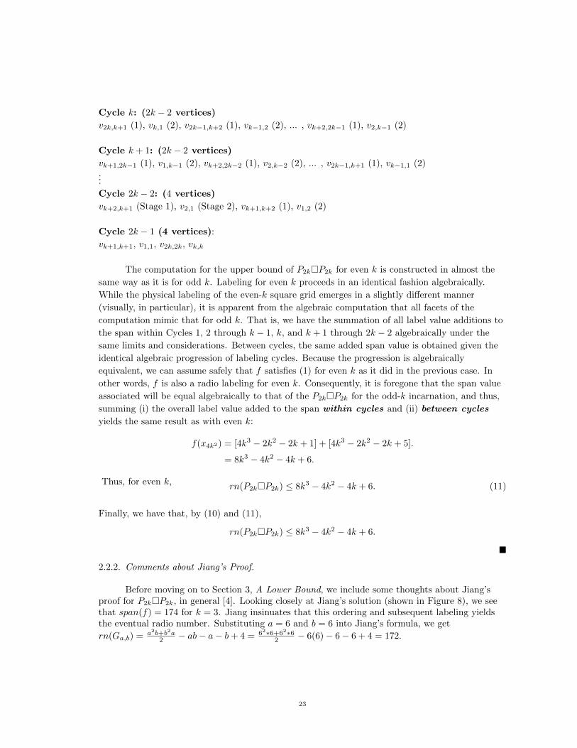
The computation for the upper bound of P2k�P2k for even k is constructed in almost the

same way as it is for odd k. Labeling for even k proceeds in an identical fashion algebraically.

While the physical labeling of the even-k square grid emerges in a slightly different manner

(visually, in particular), it is apparent from the algebraic computation that all facets of the

computation mimic that for odd k. That is, we have the summation of all label value additions to

the span within Cycles 1, 2 through k − 1, k, and k + 1 through 2k − 2 algebraically under the

same limits and considerations. Between cycles, the same added span value is obtained given the

identical algebraic progression of labeling cycles. Because the progression is algebraically

equivalent, we can assume safely that f satisfies (1) for even k as it did in the previous case. In

other words, f is also a radio labeling for even k. Consequently, it is foregone that the span value

associated will be equal algebraically to that of the P2k�P2k for the odd-k incarnation, and thus,

summing (i) the overall label value added to the span within cycles and (ii) between cycles

yields the same result as with even k:

f(x4k2) = [4k3 − 2k2 − 2k + 1] + [4k3 − 2k2 − 2k + 5].

= 8k3 − 4k2 − 4k + 6.

Thus, for even k, rn(P2k�P2k) ≤ 8k3 − 4k2 − 4k + 6. (11)

Finally, we have that, by (10) and (11),

rn(P2k�P2k) ≤ 8k3 − 4k2 − 4k + 6.

�

2.2.2. Comments about Jiang’s Proof.

Before moving on to Section 3, A Lower Bound, we include some thoughts about Jiang’sproof for P2k�P2k, in general [4]. Looking closely at Jiang’s solution (shown in Figure 8), we seethat span(f) = 174 for k = 3. Jiang insinuates that this ordering and subsequent labeling yieldsthe eventual radio number. Substituting a = 6 and b = 6 into Jiang’s formula, we get

rn(Ga,b) = a2b+b2a2 − ab− a− b+ 4 = 62∗6+62∗6

2 − 6(6)− 6− 6 + 4 = 172.

23

We can assume a few things from this inconsistency. Either Jiang’s solution s∗ is not anoptimal ordering given the demands of (1) or Jiang has neglected to necessarily include bumps inhis computation of the span. That Jiang’s radio number for all (including non-square) grids doesnot coincide with the span of his optimal labeling of even square grids may, in fact, be a typo sinceJiang shows that there is an ordering which requires 2 bumps to satisfy the radio condition onsomewhat different grounds. He also shows, after considering all possible radio labelings, thatthere is at least 1 bump for every 2 corners in the grid. Including the 2 bumps from his proof inthe computation of the radio number may be the only neglected step. We discuss bumps at greaterlength in Section 4.

Jiang’s proof demonstrates that it is possible to characterize large, abstract graphs withoutconsidering bounds on the radio number, which he accurately concludes is a simpler, morepalatable journey than “dealing with distances di, bumps bi, and labels fi simultaneously” [4].That said, Jiang also avoids directly proving that his labeling is indeed a radio labeling, which mayhave obscured his results given that (1) must also be satisfied by “higher-order,” ornon-consecutive, pairs of vertices in the ordering. Our paper instead tends to focus on the cyclicprogression of label values under an explicitly constructed and defined labeling. This affords us therelative luxury of only having to verify that distances are maximized – not that the ordering isoptimal. The contrast in styles provides an interesting account of analyzing distance inequalities,optimization problems, and abstract mappings, in general.

24

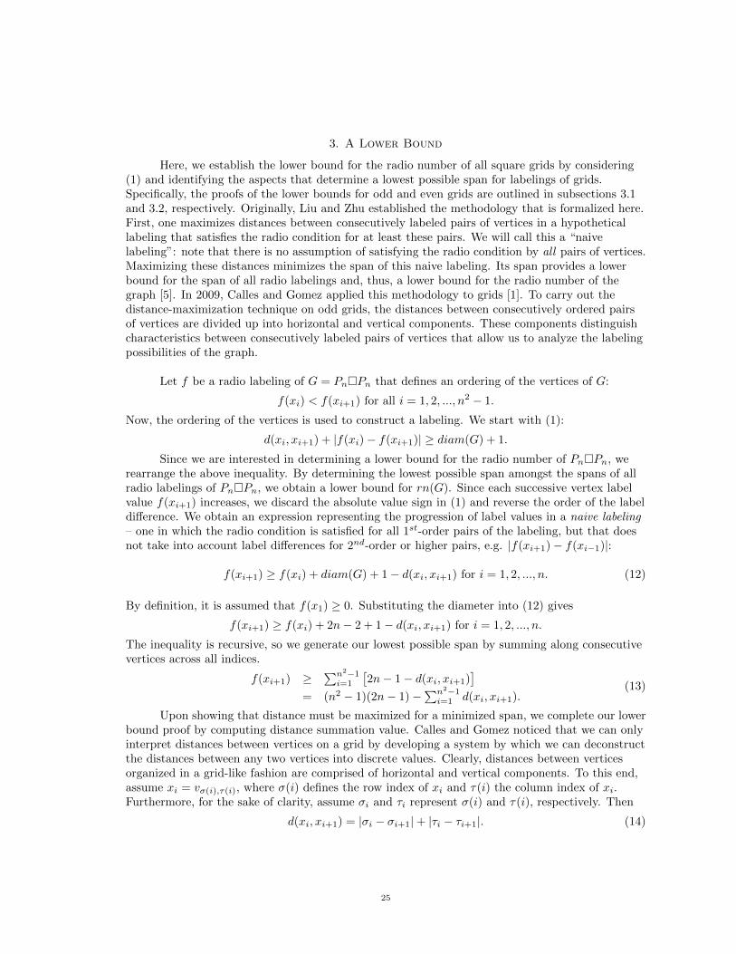
3. A Lower Bound

Here, we establish the lower bound for the radio number of all square grids by considering(1) and identifying the aspects that determine a lowest possible span for labelings of grids.Specifically, the proofs of the lower bounds for odd and even grids are outlined in subsections 3.1and 3.2, respectively. Originally, Liu and Zhu established the methodology that is formalized here.First, one maximizes distances between consecutively labeled pairs of vertices in a hypotheticallabeling that satisfies the radio condition for at least these pairs. We will call this a “naivelabeling”: note that there is no assumption of satisfying the radio condition by all pairs of vertices.Maximizing these distances minimizes the span of this naive labeling. Its span provides a lowerbound for the span of all radio labelings and, thus, a lower bound for the radio number of thegraph [5]. In 2009, Calles and Gomez applied this methodology to grids [1]. To carry out thedistance-maximization technique on odd grids, the distances between consecutively ordered pairsof vertices are divided up into horizontal and vertical components. These components distinguishcharacteristics between consecutively labeled pairs of vertices that allow us to analyze the labelingpossibilities of the graph.

Let f be a radio labeling of G = Pn�Pn that defines an ordering of the vertices of G:

f(xi) < f(xi+1) for all i = 1, 2, ..., n2 − 1.

Now, the ordering of the vertices is used to construct a labeling. We start with (1):

d(xi, xi+1) + |f(xi)− f(xi+1)| ≥ diam(G) + 1.

Since we are interested in determining a lower bound for the radio number of Pn�Pn, werearrange the above inequality. By determining the lowest possible span amongst the spans of allradio labelings of Pn�Pn, we obtain a lower bound for rn(G). Since each successive vertex labelvalue f(xi+1) increases, we discard the absolute value sign in (1) and reverse the order of the labeldifference. We obtain an expression representing the progression of label values in a naive labeling– one in which the radio condition is satisfied for all 1st-order pairs of the labeling, but that doesnot take into account label differences for 2nd-order or higher pairs, e.g. |f(xi+1)− f(xi−1)|:

f(xi+1) ≥ f(xi) + diam(G) + 1− d(xi, xi+1) for i = 1, 2, ..., n. (12)

By definition, it is assumed that f(x1) ≥ 0. Substituting the diameter into (12) gives

f(xi+1) ≥ f(xi) + 2n− 2 + 1− d(xi, xi+1) for i = 1, 2, ..., n.

The inequality is recursive, so we generate our lowest possible span by summing along consecutivevertices across all indices.

f(xi+1) ≥∑n2−1i=1

[2n− 1− d(xi, xi+1)

]= (n2 − 1)(2n− 1)−

∑n2−1i=1 d(xi, xi+1).

(13)

Upon showing that distance must be maximized for a minimized span, we complete our lowerbound proof by computing distance summation value. Calles and Gomez noticed that we can onlyinterpret distances between vertices on a grid by developing a system by which we can deconstructthe distances between any two vertices into discrete values. Clearly, distances between verticesorganized in a grid-like fashion are comprised of horizontal and vertical components. To this end,assume xi = vσ(i),τ(i), where σ(i) defines the row index of xi and τ(i) the column index of xi.Furthermore, for the sake of clarity, assume σi and τi represent σ(i) and τ(i), respectively. Then

d(xi, xi+1) = |σi − σi+1|+ |τi − τi+1|. (14)

25

Expanding (14) across all consecutive pairs of vertices in any particular labeling, a longsummation accounting for all indices of all vertices is achieved.

n2−1∑i=1

d(xi, xi+1) = |σ1 − σ2|+ |τ1 − τ2|

+ |σ2 − σ3|+ |τ2 − τ3|...

+ |σn2−1 − σn2 |+ |τn2−1 − τn2 |

(15)

Thus, the span of the labeling is constructed by combining (13) and (15) into one long inequality:

f(xn2) ≥ (n2 − 1)(2n− 1)−

(∣∣∣∣σ1 − σ2∣∣∣∣+

∣∣∣∣τ1 − τ2∣∣∣∣+...

+

∣∣∣∣σn2−1 − σn2

∣∣∣∣+ |τn2−1 − τn2

∣∣∣∣).

(16)

We refer to the above expression as the summation of distances. Each vertex contributes 4elements to the summation of distances. However, since x1 and xn2 are the first and last verticesto be labeled, respectively, the terms σ1, σn2 , τ1, and τn2 each only appear once in the summationof distances. For example, it is clear from the expansion (15) that x2 contributes a total of 4elements to the summation, but x1 contributes only 2 elements, as a result of appearing at thestart of the summation. Henceforth, the value associated with a specific arrangement will bereferred to as lost label sum λ. Therefore, 4 total lost label values – σ1, τ1, σn2 , and τn2 – willvanish as a result of corresponding to either x1 or xn2 . Of these 4 lost label values, two are positivein the above summation and two are negative. This must be considered when incorporating theseabsences from (15). Below, the process by which the lower bounds for the radio number of bothodd and even square grids is set forth.

We devise a strategy by which to maximize the sum of distances in order to minimize thespan. Calles and Gomez’s work demonstrates that it is possible to arrange index values of verticessuch that the lowest values are being subtracted and the highest added. In essence, we express thesum of distances outlined above as a difference of the sum of all positive elements and that of allnegative elements:

D =

n2−1∑i=1

d(xi, xi+1) ≤n2−1∑i=1

P −n2−1∑i=1

N, (17)

where P is the set of the highest row and column indices and N is the set of lowest row andcolumn indices for a grid Pn�Pn. When n = 2k, P = {k + 1, k + 2, ..., 2k}, while N = {1, 2, ..., k}.Similarly, for odd n = 2k+ 1, P = {k+ 2, k+ 3, ..., 2k+ 1}, while N = {1, 2, ..., k}. The index k+ 1does not yet appear in either set. We safely assume that all k + 1 index elements can be dividedevenly amongst the sets and thus cancel one another out completely.

Using the notation D to represent the sum of distances of all consecutive pairs, we canexpress a primitive incarnation (not yet having incorporated the effect of lost label values in λ) forthe maximized sum of distances with respect to odd (18) and even (19) grids as follows:

26

D =

(2k+1)2−1∑i=1

d(xi, xi+1) = 4

[2k+1∑i=k+2

i−k∑i=1

i

](18)

D =

(2k)2−1∑i=1

d(xi, xi+1) = 4

[2k∑

i=k+1

i−k∑i=1

i

](19)

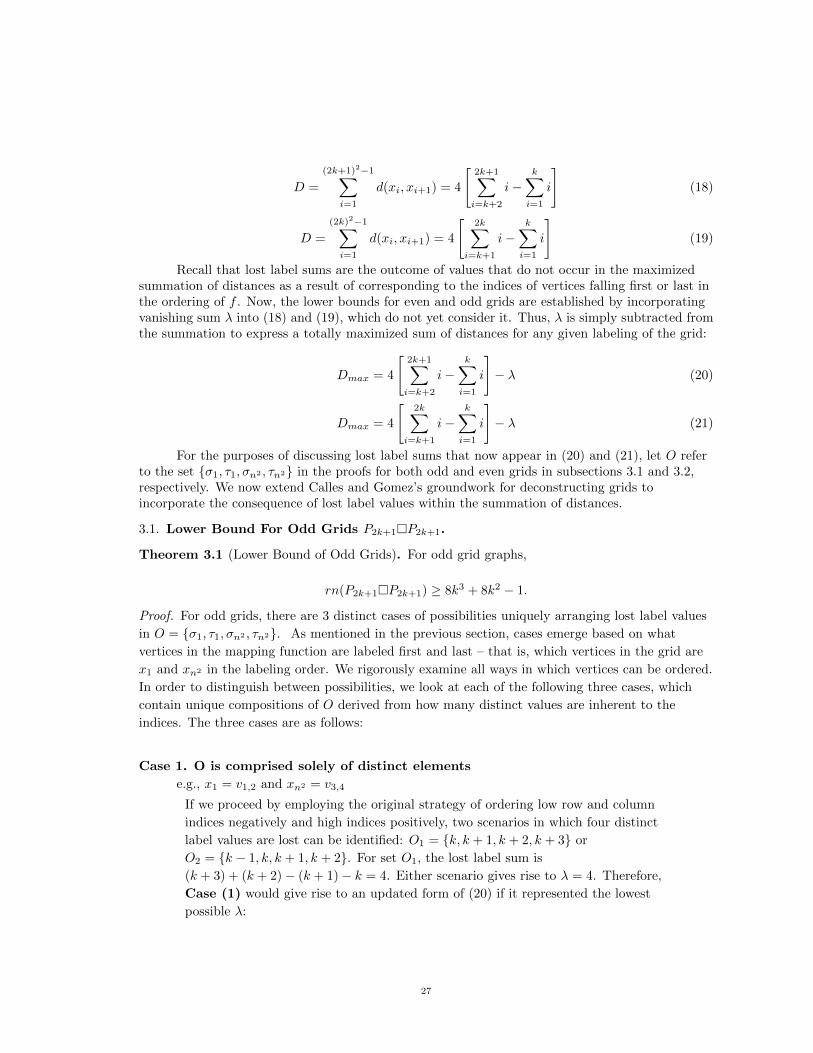
Recall that lost label sums are the outcome of values that do not occur in the maximizedsummation of distances as a result of corresponding to the indices of vertices falling first or last inthe ordering of f . Now, the lower bounds for even and odd grids are established by incorporatingvanishing sum λ into (18) and (19), which do not yet consider it. Thus, λ is simply subtracted fromthe summation to express a totally maximized sum of distances for any given labeling of the grid:

Dmax = 4

[2k+1∑i=k+2

i−k∑i=1

i

]− λ (20)

Dmax = 4

[2k∑

i=k+1

i−k∑i=1

i

]− λ (21)

For the purposes of discussing lost label sums that now appear in (20) and (21), let O referto the set {σ1, τ1, σn2 , τn2} in the proofs for both odd and even grids in subsections 3.1 and 3.2,respectively. We now extend Calles and Gomez’s groundwork for deconstructing grids toincorporate the consequence of lost label values within the summation of distances.

3.1. Lower Bound For Odd Grids P2k+1�P2k+1.

Theorem 3.1 (Lower Bound of Odd Grids). For odd grid graphs,

rn(P2k+1�P2k+1) ≥ 8k3 + 8k2 − 1.

Proof. For odd grids, there are 3 distinct cases of possibilities uniquely arranging lost label values

in O = {σ1, τ1, σn2 , τn2}. As mentioned in the previous section, cases emerge based on what

vertices in the mapping function are labeled first and last – that is, which vertices in the grid are

x1 and xn2 in the labeling order. We rigorously examine all ways in which vertices can be ordered.

In order to distinguish between possibilities, we look at each of the following three cases, which

contain unique compositions of O derived from how many distinct values are inherent to the

indices. The three cases are as follows:

Case 1. O is comprised solely of distinct elements

e.g., x1 = v1,2 and xn2 = v3,4

If we proceed by employing the original strategy of ordering low row and column

indices negatively and high indices positively, two scenarios in which four distinct

label values are lost can be identified: O1 = {k, k + 1, k + 2, k + 3} or

O2 = {k − 1, k, k + 1, k + 2}. For set O1, the lost label sum is

(k + 3) + (k + 2)− (k + 1)− k = 4. Either scenario gives rise to λ = 4. Therefore,

Case (1) would give rise to an updated form of (20) if it represented the lowest

possible λ:

27

(2k+1)2−1∑i=1

d(xi, xi+1) = 4

[2k+1∑i=k+2

i−k∑i=1

i

]− 4 (22)

Case 2. O is comprised of exactly 3 distinct elements

e.g., x1 = v1,2 and xn2 = v3,2

In Case (2), there are three distinct elements in O. Thus, two distinct values are

lost once each and the other twice. Recall that low values should be negative,

while high values should be positive. Only two possible sets emerge:

O1 = {k, k + 1, k + 1, k + 2} or O2 = {k − 1, k, k, k + 1}. Again, in each case, one

middle value is defined to be positive, the other negative. In either scenario, λ = 2.

Case 3. O is comprised of exactly 2 distinct elements

There are precisely two possible subcases that arise:

Subcase 3.A. Each distinct element is repeated once

e.g., x1 = v1,1 and xn2 = v3,3

Considering that k + 1 is the undistributed value for an odd grid, it is necessary to

place k + 1 in O. We have two possibilities: O1 = {k, k, k + 1, k + 1} and

O2 = {k + 1, k + 1, k + 2, k + 2}. Adding up negative and positive values yields

λ = 2 for each set.

Subcase 3.B. 1 element is repeated 3 times, the other element just once

e.g., x1 = v2,2 and xn2 = v2,4

We can arrange indices so that k disappears three times or so that k+ 1 disappears

three times. From these two options arise three distinct sets: O1 = {k, k, k, k + 1},O2 = {k, k + 1, k + 1, k + 1}, and O3 = {k + 1, k + 1, k + 1, k + 2}. After making

two high elements positive and two low elements negative, it is clear that each set

results in λ = 1.

It is worthwhile to take note that O cannot consist of just one distinct element as this would

require labeling the same vertex twice. Thus, it is now possible to definitively choose an

arrangement in which the lost label value λ is minimized in order to maximize∑d(xi, xi+1). This

occurs in Case 3.B. We now obtain an updated form of (20) for the maximum sum of distances:

(2k)2−1∑i=1

d(xi, xi+1) = 4

[2k∑

i=k+1

i−k∑i=1

i

]− 1 (23)

Recall that there is an extra multiplicative factor of (2k + 1) in the updated portion of the

maximized distances due to the fact that there are four total cases of each row or column index

appearing in the maximized distance formula, but over the span of the entire graph, this must

occur for each of 2k + 1 rows (or columns).

28

f(x4k2−1) ≥[(2k + 1)2 − 1

](4k + 1)−

[4(2k + 1)

( ∑2k+1i=k+2 i−

∑ki=1 i

)− 1]

Using summation formulas, the inequality is reduced to:

f(x4k2−1) ≤ 4k(k + 1)(4k + 1)− 4k(2k + 1)(k + 1)− 1

= (k + 1)(4k)(2k)− 1

= 8k2(k + 1)− 1.

f(x4k2−1) ≥ 8k3 + 8k2 − 1 (24)

Thus, the lower bound is attained:

rn(P2k+1�P2k+1) ≥ 8k3 + 8k2 − 1.

�

3.2. Lower Bound For Even Grids P2k�P2k.

Theorem 3.2 (Lower Bound of Even Grids). For even grids,

rn(P2k�P2k) ≥ 8k2 − 4k2 − 4k + 2.

Proof. The proof is analogous to that of the odd case.

Case 1. O is comprised solely of distinct elements

e.g., x1 = v1,2 and xn2 = v3,4

O becomes {k − 1, k, k + 1, k + 2}. When the elements of O are summed (again

remembering to use low indices negatively and high indices positively), λ = 4, as in

the odd case.

Case 2. O is comprised of exactly 3 distinct elements

e.g., x1 = v1,2 and xn2 = v3,2

Then O1 = {k− 1, k, k, k+ 1} or O2 = {k− 1, k, k+ 1, k+ 1}. In either case, λ = 2.

Case 3. O is comprised of exactly 2 distinct elements

Again, precisely two possible subcases emerge:

Subcase 3.A. Each distinct element is repeated once

e.g., x1 = v1,1 and xn2 = v3,3

O1 = {k, k, k + 1, k + 1}. Adding up negative and positive values results in a lost

label sum λ = 2.

Subcase 3.B. 1 element is repeated 3 times; the other element just once

e.g., x1 = v2,2 and xn2 = v2,4

O1 = {k, k, k, k + 1} or O2 = {k, k + 1, k + 1, k + 1}. In either case, λ = 1.

Of the three cases for even grids, Case 3.B provides the lowest lost label sum. We represent the

maximized sum of distances for even grids by updating (21) with λ = 1:

29

(2k)2−1∑i=1

d(xi, xi+1) = 4

[2k∑

i=k+1

i−k∑i=1

i

]− 1. (25)

The effective span, f(xn2), is then computed for an even grid with a maximum sum of

distances by substituting the above into (13) and simplifying. Again, a multiplicative factor of 2k

must be included to represent the emergence of row and column indices over the 2k rows (or

columns) of the grid.

f(x4k2) ≥[(2k)2 − 1

](4k − 1)−

[4(2k)

( ∑2ki=k+1 i−

∑ki=1 i

)− 1].

Using summation formulas gives us

f(x4k2) ≥ [4k2 − 1)(4k − 1)− (8k3 − 1)

= 16k3 − 4k2 − 4k + 1− 8k3 + 1

= 8k3 − 4k2 − 4k + 2.

Since span(f) = f(x4k2),

span(f) ≥ 8k3 − 4k2 − 4k + 2,

and the lower bound is attained:

rn(P2k�P2k) ≥ 8k3 − 4k2 − 4k + 2. (26)

�

30

Figure 9. Quadrants of P6�P6 with diagonal triple {xi−1, xi, xi+1}

4. The “Bump”

For the remainder of analysis, let the following definitions and assumptions apply.

• Let G = P2k�P2k.

• Let f be some labeling of a graph H. Define {x1, x2, ..., xn} to be an ordering of thevertices of H such that f(xi) < f(xi+1) for i = 1, 2, ...n− 1.

• Define vertex label xi = vσ(i),τ(i), where σ(i) defines the row index of xi and τ(i) thecolumn index of xi. Furthermore, for the sake of clarity, assume σi and τi represent σ(i)and τ(i), respectively.

• Without loss of generality, assume f(x1) = 0.

• Define f to be a naive labeling if f(xi) = f(xi−1) + diam(G) + 1− d(xi, xi−1).

• The term “bump” will be used to refer to the increase in the span of a naive labelingrequired to ensure that the labeling satisfies the radio condition (1) for some nth-order pairof vertices.

• An even grid can be subdivided into four quadrants, defined as Q1, Q2, Q3, and Q4 aslabeled in Figure 1. Define diagonally opposite quadrants as one of the followingquadrants pairs: (Q1, Q3) or (Q2, Q4) – e.g., Q1 and Q3 are diagonally oppositequadrants. Define adjacent quadrants as a pair of quadrants having the characteristic ofnot being diagonally opposite to one another – e.g., Q1 and Q2 are adjacent quadrants(see Figure 8).

Proposition 1 (Diagonal Triple). Let G be an even grid P2k�P2k. Let f be a naive labeling of G

with ordering {x1, x2, ..., xn} defined by f . Let f∗ be any radio labeling inducing the same

ordering {x1, x2, ..., xn} on the vertices of G. Say xi−1 and xi+1 are vertices in a diagonally

opposite quadrant. Then,

f∗(xi+1)− f∗(xi−1) ≥ f(xi+1)− f(xi−1) + 1, (27)

31

for any 3 consecutively labeled vertices xi−1, xi, and xi+1 as defined above.

Proof. Let G, f∗, and f be as hypothesized. By applying the definition of naive labeling f and

considering restrictions placed on τ and σ values, we will show that the difference of label values

between 2nd-order pairs of vertices requires a “bump” of +1 for f to be a radio labeling. Our naive

labeling conveys that f(xi) = f(xi−1) + diam(G) + 1− d(xi, xi−1), so after inserting the diameter,

f(xi) = f(xi−1) + 4k − 1− d(xi, xi−1).

Similarly,

f(xi+1) = f(xi) + 4k − 1− d(xi+1, xi).

After substitution,

f(xi+1) = f(xi−1) + 8k − 2− [d(xi, xi−1) + d(xi+1, xi)]. (28)

It is important to establish conditions that will govern analysis of our designated set of

vertices. Since we have a 2nd-order pair of vertices xi−1 and xi+1 in one quadrant and another

vertex xi in a diagonally opposite quadrant, it is advantageous to relate their placement in the grid

to their row and column indices. So, assume without loss of generality that the following

conditions hold and are referred to as our quadrant inequalities:

τi−1, σi−1 ∈ P,τi+1 ≤ τi−1,

σi+1 ≤ σi−1

(29)

Set restrictions on relative row and column indices of vertices part of the same triple such that

they abide by quadrant inequalities (29) as follows:

|τi+1 − τi| ≥ k ±∆,

|σi+1 − σi| ≥ k ∓∆,(30)

where ∆ is the value associated with distance between consecutive vertices that causes any

deviation from a naive labeling.

Upon setting restrictions on τ and σ, we examine the sum of distances closely.

d(xi, xi−1) + d(xi+1, xi) = |σi − σi−1|+ |τi − τi−1|+ |σi+1 − σi|+ |τi+1 − τi|= σi−1 − σi + τi−1 − τi + σi+1 − σi + τi+1 − τi= σi−1 + σi+1 − 2σi + τi−1 + τi+1 − 2τi.

We add 2σi+1 − 2σi+1 + 2τi+1 − 2τi+1 to rearrange the equality and substitute for

expressions that permit us to characterize particular relationships that exist within the grid.

Continuing the equality established with a more useful form of the right side, we have

d(xi, xi−1) + d(xi+1, xi) =[σi−1 − σi+1

]+ 2σi+1 − 2σi +

[τi−1 − τi+1

]+ 2τi+1 − 2τi

= 2(σi+1 − σi) + 2(τi+1 − τi) +[(σi−1 − σi+1) + (τi−1 − τi+1)

].

Noting carefully that (σi−1 − σi+1) + (τi−1 − τi+1) is really just the distance between 2nd-order

pairs of vertices xi−1 and xi+1, we can establish a final equality that captures the evolution of the

32

naive labeling at the outset into a distance expression that relates both a 1st-order pair as well as a

2nd-order pair of vertices. Substituting (30),

d(xi, xi−1) + d(xi+1, xi) = 2(σi+1 − σi) + 2(τi+1 − τi) + d(xi−1, xi+1)

≥ 4k ± 2∆∓ 2∆ + d(xi−1, xi+1).

≥ 4k + d(xi−1, xi+1).

Substituting the above into (28) yields an inequality characterizing 2nd-order pairs of vertices:

f(xi+1) ≤ f(xi−1) + 8k − 2− 4k − d(xi−1, xi+1).

Reorganizing gives rise to an inequality reflecting the relationship between 2nd-order pairs of

vertices constrained by quadrant inequalities (29):

f(xi+1)− f(xi−1) + d(xi−1, xi+1) ≤ 4k − 2.

(1) mandates that, for any pair of vertices u and v in P2k�P2k, |f(u)− f(v)|+ d(u, v) ≥ 4k − 1.

Therefore, the result of Proposition 1 demonstrates that the value f(xi−1) is 1 too low for f to be

a radio labeling of an even grid G. �

Henceforth, define any set of 3 consecutively labeled vertices in the above configuration tobe a diagonal triple. Since we employ a naive labeling, the radio condition is satisfied for pairs inthe above configuration, but is not necessarily fulfilled for 2nd-or-higher-order pairs of vertices.Thus, we have shown that a typical naive labeling for an even grid structure will not necessarilysatisfy the radio condition. We will use this to show that (i) the lower bound for rn(P2k�P2k)must be at least 2 higher, and (ii) that the lower bound may in fact also require several “bumps”of various kinds in order to define a radio labeling. Lemma 1 builds on the latter, detailing how theeffect of this kind of vertex triplet in an even grid rules out many kinds of labelings and ultimatelyhelps determine the lowest span of a viable radio labeling for an even grid G.

Recall, from Section 3, that the distance-maximizing labeling used to construct the lowerbound for rn(P2k�P2k) is not necessarily a radio labeling. We show that radio labelings of gridsare forms of “adjusted distance-maximizing labelings” that abide by radio condition (1) at alltimes. First, it is necessary re-define distance-maximizing labeling to clarify how optimal spansrelate to naive labelings of even grids. In Section 3, we demonstrate that we can obtain maximizeddistances between consecutively labeled vertices by making higher σ and τ index values positiveand lower σ and τ values negative. In Section 3.2, we see that there are many possible spans withmaximized distances due to vanishing index values, and consequently, different λ values arise.Henceforth, refer to distance-maximizing labelings as an ordering of vertices with thecharacteristics specified in Section 3.2. Let S = 8k3 − 4k2 − 4k + 2. Thus, for anydistance-maximizing labeling f , span(f) ∈ {S, S + 1, S + 3} corresponding to λ ∈ {1, 2, 4},respectively.

For the purposes of Lemma 1 below, define A to be a set of independent diagonal triples if no twodiagonal triples in A share more than one vertex.

33

Lemma 1 (α independent diagonal triples). Let G be an even grid. Let c0 be a

distance-maximizing and naive labeling with ordering {x1, x2, ..., xn} defined by c0 and let c∗ be a

radio labeling inducing the same ordering {x1, x2, ..., xn} on the vertices of G.

span(c∗) ≥ span(c0) + α. (31)

where α is the size of the largest set A associated with labeling c∗ of G.

Proof. Say xi−1, xi, xi+1, xi+2, and xi+3 constitute 3 consecutively labeled diagonal triples in the

ordering patterns of labeling co and radio labeling c∗ of an even grid G.

Then, by Proposition 1, c∗(xi+1)− c∗(xi−1) ≥ c0(xi+1)− c0(xi−1) + 1.

Proposition 1 does not require that c∗(xi+2)− c∗(xi) ≥ c0(xi+2)− c0(xi) + 1.

However, Proposition 1 does imply that c∗(xi+3)− c∗(xi+1) ≥ c0(xi+3)− c0(xi+1) + 1.

Vertex triplets (xi−1, xi, xi+1) and (xi+1, xi+2, xi+3) are independent diagonal triples. Then,

each element of the largest set A associated with a radio labeling c∗ contributes a “bump” of +1 to

the span of any radio labeling relative to that of a distance-maximizing labeling with the same

ordering. Therefore,

span(c∗) ≥ span(c0) + α.

�

Remark 2. Since, in any distance-maximizing and naive labeling, there are 2 sets of vertices that

satisfy the conditions set forth in Lemma 1 and quadrant inequalities (29), we can infer, without

loss of generality, that, up to permutations, there is at least 1 diagonal triple for each of diagonal

quadrant pairs (Q1, Q3) and (Q2, Q4). Thus, we have at least a bump of +2 resulting from

independent diagonal triples in a distance-maximizing, naive labeling – that is, α ≥ 2.

Remark 2 confirms that there are multiple bumps associated with a radio labeling ofP2k�P2k. The following discussions regarding “adjacent flips” demonstrates a diagonal triple is notthe only source of bumps. Before stating Lemma 2, we define the meaning of adjacent flip. Anadjacent flip is the occurrence of any consecutively labeled pair of vertices in adjacent quadrants.Thus, an adjacent flip represents one of two possibilities: (a) xi is in either Q1 or Q3 and xi+1 is ineither Q2 or Q4 or (b) xi is in Q2 or Q4 and xi+1 is in either Q1 or Q3.

Lemma 2 (β adjacent flips). Let G be an even grid. Let c0 be a distance-maximizing and naive

labeling with ordering {x1, x2, ..., xn} defined by c0 and let c∗ be a radio labeling inducing the

same ordering {x1, x2, ..., xn} on the vertices of G. Then,

span(c∗) ≥ span(c0) + 2 · β, (32)

where β is the number of adjacent flips that occur in the complete labeling of G under c∗.

Proof. Let G be an even grid and c0 a distance-maximizing labeling of G. Define D0, P0, and N0

as in (17) corresponding to labeling c0. Thus, P0 and N0 represent the sets of largest and smallest

row and column indices, respectively, in D0, for a distance-maximizing labeling c0. Also, define D∗

34

as the equivalent for radio labeling c∗.

Consider exchanging the smallest element in P0 with the largest element in N0, while

preserving all other elements of P0 and N0. This can be thought of as making the smallest possible

concession in deviating from the distance-maximizing labeling c0. As the largest element in N0 is k

and the smallest in P0 is k + 1, exchanging these elements results in replacing +(k + 1)− k with

+k − (k + 1) in the maximized sum of distances for labeling c∗. Thus, each adjacent flip results in

an increase of at least 2 in the span of the resulting labeling, so D∗ = D0 - 2. The statement

follows directly. �

Remark 3. Notice that any complete labeling of P2k�P2k must include at least one adjacent flip.

Thus, β ≥ 1. This necessitates an additional bump of at least +2 to any complete radio labeling of

an even grid and, more specifically, in relation to the span of any distance-maximizing labeling

that constructs a lower bound for the graph.

Finally, we associate a change in the span of any radio labeling corresponding to α diagonaltriples and β adjacent flips in Lemma 3 below.

Lemma 3 (α independent diagonal triples and β adjacent flips). Let G be an even grid. Let c0 be

a distance-maximizing and naive labeling with ordering {x1, x2, ..., xn} defined by c0 and let c∗ be

a radio labeling inducing the same ordering {x1, x2, ..., xn} on the vertices of G. If c∗ contains α

independent diagonal triples and β adjacent flips, then

span(c∗) ≥ span(c0) + α+ 2 · β. (33)

Proof. Given that any distance-maximizing and naive labeling of G contains adjacent flips and

independent diagonal triples, we note that independent diagonal triples and adjacent flips are

independent of one another, and Lemma 3 follows directly from Lemmas 1 and 2. �

We see in Section 3.2 that we can construct a lower bound for the radio number of evengrids by considering all naive labelings. We also observe that distance-maximizing labelings havethe lowest spans of all naive labelings. Since we choose only one of the distance-maximizing, naivelabelings to produce a lowest possible span S (there are numerous arrangements with λ = 1), it isnecessary to show that all other distance-maximizing, naive labelings have spans that must bebumped up sufficiently in order to be radio labeling. Thus, we eliminate the spans arising fromother distance-maximizing, naive labelings corresponding to unique values λ ∈ {1, 2, 4}. and showthat any naive labeling must have its span bumped up sufficiently to be radio labeling.

Corollary 1 (Minimum bump moves). Let G be an even grid. Let c0 be a distance-maximizing

and naive labeling with ordering {x1, x2, ..., xn} defined by c0 and let c∗ be a radio labeling

inducing the same ordering {x1, x2, ..., xn} on the vertices of G. Then

α+ β ≥ 3 (34)

Proof. Section 3.2 shows that we can have many possible naive labelings of G given different λ

values. By contrast, Remarks 1 and 2 show that, regardless of labeling arrangement, any

distance-maximizing and naive labeling of G must contain at least 2 independent diagonal triples

and 1 adjacent flip. Thus, α ≥ 2 and β ≥ 1. The statement follows directly. �

35

Corollary 2 (Minimum span of a distance-maximizing radio labeling of P2k�P2k). Let G be an

even grid. Let c0 be a distance-maximizing and naive labeling with ordering {x1, x2, ..., xn} defined

by c0 and let c∗ be any radio labeling inducing the same ordering {x1, x2, ..., xn} on the vertices of

G. Then

span(c∗) ≥ span(c0) + 4. (35)

Proof. The statement follows directly from Lemma 3 and Corollary 1. �

With Corollaries 1 and 2 now in place, we determine the radio number of all even grids. We haveshown that a distance-maximizing and naive labeling of an even grid requires numerous bumps inorder to be a radio labeling. In Theorem 4, we eliminate all labelings whose span exceeds ourupper bound for the radio number and thus determine the radio number to be the span of Jiang’seven grid labeling.

Theorem 4 (Radio number of even square grids). Let G = P2k�P2k. Let f∗ be a naive labeling

of G. Let f be a radio labeling of G. The radio number of an even square grid is given by

rn(P2k�P2k) = 8k3 − 4k2 − 4k + 6.

Proof. Let S = 8k3 − 4k2 − 4k + 2. Theorem 3.2 proves that the lowest possible span of any

naive labeling is S. The distance-maximizing approach employed in Section 3 shows that

distance-maximizing labelings have the lowest spans of all naive labelings. Suppose f∗ has a span

in {S, S + 1, S + 3}. Corollary 2 proves that any radio labeling f of G must have a span of at

least S + 4.

Theorem 2.2 proves an upper bound for the radio number:

span(f) ≤ 8k3 − 4k2 − 4k + 6.

Closing bounds on rn(P2k�P2k) gives us

S + 4 ≤ span(f) ≤ 8k3 − 4k2 − 4k + 6.

Thus, span(f) = rn(G) = 8k3 − 4k2 − 4k + 6, as required. �

36

5. Observations and Future Research

An investigation of the radio number of grids brings to light many important results. Firstand foremost, it relates the value of certain techniques in exploring highly specialized Cartesianproducts. In other words, it is seen how the structure of any abstract graph can affect how thatgraph must abide by certain constraints and the ways in which it can even be analyzed.

Calles and Gomez lay the groundwork for applying bounded approaches in determiningradio numbers of grids. Their inspiration becomes the focus of another endeavor entirely, namely acommentary on what shortcomings bounded approaches have in accomplishing this task. It is seenin [4] that labeling functions geared at capturing “radio characteristics” of specific graphs may betoo indirect for some examples in the space of graph structure analysis. Jiang’s labeling itselfechoes of the inherent bound-reconciling analysis that is required in Jiang’s overall approach, butreduces the problem to optimization. He shows that it is possible to circumvent conventionalbounding techniques and avoid the pitfalls of balancing the various demands of distances, bumps,and labelings (or orderings) under (1). It is also clear that bump analysis is not inherently linkedto bounded approaches. In this paper, however, it is shown that bump analysis does in factparallel bound construction itself. Similarly, exhaustive fulfillment of (1) under algebraicconstraints requires an eventual choice in analytical paths.

Those who are interested in pursuing other avenues in this field might consider applying thetechniques illustrated here for the immediate purpose of finding rn(P2k+1�P2k+1) usingconventional bounding approaches. While the exact same strategy used here may not provefruitful, the approach outlined in this paper provides a strong basis by which to examine squaregrids. When considering the fact that grids, like numerous other families of graphs, are really justproducts of simpler graphs, it is likely that one may extend the findings in this paper suitably toodd grids. An odd grid additionally contains an even grid and two more paths (one extra row andone extra column). This itself, may be a solid enough base with which to determine the radionumber of odd grids by applying Lemma 3 and Proposition 1 rigorously. Likewise, it is a naturalpossibility to investigate Cartesian products of grids and other graphs while incorporating some ofthe abstract considerations established here, as well as in [4] and [5].

The methodologies employed within this paper intend to capture the nature of thesometimes nebulous field of radio labeling. Networks of radio transmitters tie in closely with theidea of graph theory because their arrangements transcend the rigid constraints of just a singularcharacteristic. Instead, investigating the radio number of abstract graph structures that possessnumerous, and often disparate, structural components leads to a great deal of insight about howabstract graph families preserve overall form. We know that, in the real world, the study ofnetworks and inter-connectivity is of profound significance and the interplay between overallstructure and internal chaos is manifest in global systems. Hopefully, in addition to commentingsuccessfully about the radio number of square grids, this paper will develop into a source ofknowledge about applying analytical techniques for the exploration of all kinds of networks andstructures around us. Although it may seem like a daunting task, graph properties and structurecorrespond so fundamentally to the radio labelings of graphs that linking properties such asdiameter, adjacency, or chromatic number is both a rich source of both future progress in graphtheory and combinatorics, as well as relatively unprobed territory with considerable potential inmodern physics and applied mathematics.

37

References

[1] Calles, Eduardo and Gomez, Henry, Radio Labeling Grid Graphs. Paper presented at: Joint Mathematics

Meetings; Jan. 5-8, 2009. Washington, D.C.

[2] G. Chartrand and Erwin, David and Zhang, Ping and Harary, Frank Radio labelings of graphs, Bull Inst.

Combin. Appl., 33 (2001), pp. 77-85.

[3] G. Chartrand, D. Erwin, and P. Zhang A graph labeling problem suggested by FM channel restrictions, Bull

Inst. Combin. Appl., 43 (2005), pp. 43-57.

[4] Jiang, T.-S. A. The Radio Number of Grid Graphs, arXiv e-prints, Jan. 2014, arXiv:1401.6583.

[5] Liu, Daphne Der-fen and Zhu, Xuding Multi-level distance labelings for paths and cycles, Siam J. Discrete

Math., 19 (1993), pp. 610-621.

38