Big Data Analysis

Matt Taddy, University of Chicago Booth School of Business

faculty.chicagobooth.edu/matt.taddy/teaching

Outline

What is [good] data mining? Discovery without overfit.

For most of today, it is variable selection in high dimensions.

Three ingredients to model building:

Model metrics: False Discovery proportion, Out-of-sample

deviance, model probabilities.

Estimation of these metrics: FD Rate control, n-fold

cross validation, and information criteria.

Building sets of candidate models: p-value cut-offs,

stepwise regression, regularization paths.

If there is time we can discuss factor models and PCR.

1

An example: Comscore web data

Detailed information about browsing and purchasing behavior.

100k households, 60k where any money was spent online.

I’ve extracted info for the 8k websites viewed by at least 5%.

Why do we care? Predict consumption from browser history.

e.g., to control for base-level spending, say, in estimating

advertising effectiveness. You’ll see browser history of users

when they land, but likely not what they have bought.

Thus predicting one from the other is key.

Potential regressions: p($ > 0|x) or E[log $|$ > 0,x].

x is just time spent on different domains. It could also include

text or images on those websites or generated by the user

(facebook) or their friends... data dimension gets huge fast.

2

DM is discovering patterns in high dimensional data

Data is usually big in both the number of observations (‘n’)

and in the number of variables (‘p’), but any p ≈ n counts.

In scientific applications, we want to summarize HD data in

order to relate it to structural models of interest.

⇒ interpretable variables or factors, causal inference.

We also want to predict! If things don’t change too much...

⇒ sparse or low-dimensional bases, ensemble learning.

The settings overlap and have one goal: Dimension Reduction.

3

Model Building: Prediction vs Inference

In some sense it is all about prediction.

Predictive modeling to forecast y | xwhere both are drawn from some joint p(y,x).

Causal modeling to forecast y | d,xwhen d moves but x is held constant.

In the former, DR is ‘in the direction’ of y. In the latter, DR is

in the direction of specific parameters in structural models.

You need to walk before you can run: good prediction is a

pre-req for causal inference. For example, one ‘controls for’ x

by building predictive each of y|x and d|x.

Everything requires a different approach when n ≈ p are big.

4

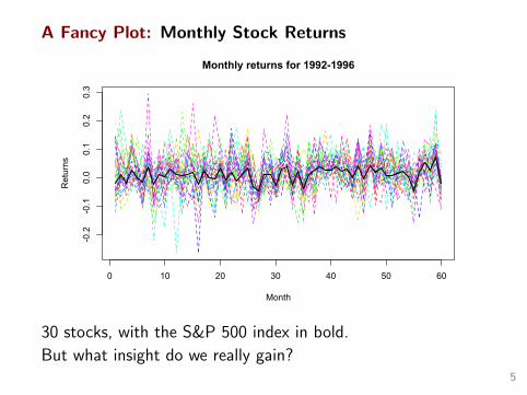
A Fancy Plot: Monthly Stock Returns

0 10 20 30 40 50 60

-0.2

-0.1

0.0

0.1

0.2

0.3

Monthly returns for 1992-1996

Month

Returns

30 stocks, with the S&P 500 index in bold.

But what insight do we really gain?5

A Powerful Plot: S&P Market Model Regression

CAPM regresses returns on the “market”: R ≈ α + βM .

0.6 0.8 1.0 1.2 1.4 1.6 1.8

-0.010

0.000

0.010

0.020

Market CAPM

beta

alpha AA

ALD

AXP

BACAT

CHVDD DIS

EKENE

GEGM

GT

HWP

IBM

IPJNJJPM

KO

MCD

MMM

MO

MRK

PG

S TRV

UK

UTX

WMT

XON

CAPM is great predicitive DM and, with factor interpretation

through the efficient market story, it is also a structural model.6

Model and Variable Selection

DM is the discovery of patterns in high dimensions.

Good DM is on constant guard against false discovery.

False Discovery = Overfit: you model idiosynchratic noise

and the resulting predictor does very poorly on new data.

The search for useful real patterns is called model building.

In linear models, this is a question of ‘variable selection’.

Given E[y|x] = f(x′β), which βj are nonzero?

Linear models dominate economics and we focus on variable

selection. Since x can include arbitrary input transformations

and interactions, this is less limiting than it might seem.

7

All there is to know about linear models

The model is always E[y|x] = f(xβ).

I Gaussian (linear): y ∼ N(xβ, σ2).

I Binomial (logistic): p(y = 1) = exβ/(1 + exβ).

I Poisson (log): E[y] = var(y) = exp[x′β].

β is commonly fit to maximize LHD ⇔ minimize deviance.

The likelihood (LHD) is p(y1|x1)× p(y2|x2) · · · × p(yn|xn).

The deviance at β is 2log(saturatedLHD) - 2 logLHD(β).

Fit is summarized by R2 = 1− dev(β)/dev(β = 0).

EG, linear regression deviance is the sum of squares and

R2 = 1− SSE/SST is the ‘proportion of variance explained’.

In DM the only R2 we ever care about is out-of-sample R2.8

Semiconductor Manufacturing Processes

Very complicated operation

Little margin for error.

Hundreds of diagnostics

Useful or debilitating?

We want to focus reporting

and better predict failures.

x is 200 input signals, y has 100/1500 failures.

Logistic regression for failure of chip i is

pi = p(faili|xi) = eα+xiβ/(1 + eα+xiβ)

The xij inputs here are actually orthogonal: they are the first

200 Principal Component directions from an even bigger set.9

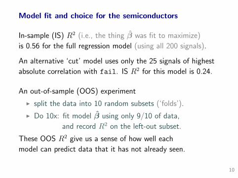
Model fit and choice for the semiconductors

In-sample (IS) R2 (i.e., the thing β was fit to maximize)

is 0.56 for the full regression model (using all 200 signals).

An alternative ‘cut’ model uses only the 25 signals of highest

absolute correlation with fail. IS R2 for this model is 0.24.

An out-of-sample (OOS) experiment

I split the data into 10 random subsets (‘folds’).

I Do 10x: fit model β using only 9/10 of data,

and record R2 on the left-out subset.

These OOS R2 give us a sense of how well each

model can predict data that it has not already seen.

10

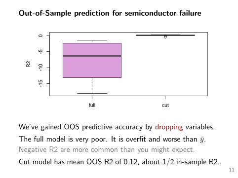
Out-of-Sample prediction for semiconductor failure

full cut

-15

-10

-50

model

R2

We’ve gained OOS predictive accuracy by dropping variables.

The full model is very poor. It is overfit and worse than y.

Negative R2 are more common than you might expect.

Cut model has mean OOS R2 of 0.12, about 1/2 in-sample R2.11

Our standard tool to avoid false discovery is hypothesis testing.

Hypothesis Testing: a one-at-a-time procedure.

Recall: p-value is probability of getting a test statistic farther

into the distribution tail than what you observe: P (Z > z).

Testing procedure: Choose a cut-off ‘α’ for your p-value ‘p’,

and conclude significance (e.g., variable association) for p < α.

This is justified as giving only α probability of a false-positive.

For example, in regression, β 6= 0 only if its p-value is less

than the accepted risk of a false discovery for each coefficient.

12

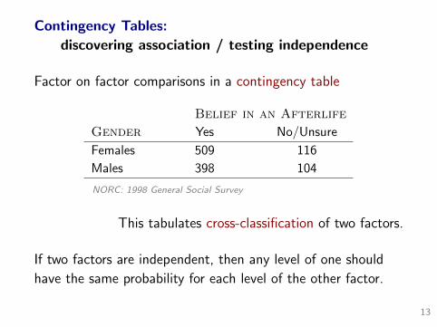
Contingency Tables:

discovering association / testing independence

Factor on factor comparisons in a contingency table

Belief in an Afterlife

Gender Yes No/Unsure

Females 509 116

Males 398 104

NORC: 1998 General Social Survey

This tabulates cross-classification of two factors.

If two factors are independent, then any level of one should

have the same probability for each level of the other factor.

13

Review: Pearson chi-squared tests for independence

Consider a table with i = 1...I rows and j = 1...J columns.

If the two factors are independent, expected cell counts are

Eij = row.totali × column.totalj/N . and the statistic

Z =∑i

∑j

(Nij − Eij)2

Eij

has χ2 distribution with df = (I−1)(J−1) degrees of freedom.

The continuity approximation that requires Eij ≥ 5ish. Some

software make small changes, but this is the basic formula.

14

Independence of Sex and the Afterlife

z =(509− 503)2

503+

(398− 404)2

404+

(116− 122)2

122+

(104− 98)2

98≈ 0.8

0 1 2 3 4 5

0.0

0.5

1.0

1.5

z

dchi

sq(z

, 1)

z = 0.82

qchisq(.95,1)

No association between gender and afterlife beliefs.

15

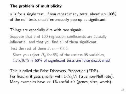
The problem of multiplicity

α is for a single test. If you repeat many tests, about α×100%

of the null tests should erroneously pop up as significant.

Things are especially dire with rare signals:

Suppose that 5 of 100 regression coefficients are actually

influential, and that you find all of them significant.

Test the rest of them at α = 0.05:

Since you reject H0 for 5% of the useless 95 variables,

4.75/9.75 ≈ 50% of significant tests are false discoveries!

This is called the False Discovery Proportion (FDP).

For fixed α it gets smaller with 1-N0/N (true non-Null rate).

Many examples have << 1% useful x’s (genes, sites, words).

16

The False Discovery Rate

Instead of focusing on each test, we’ll consider

FD Proportion =# false positives

# tests called significant

FDP is a property of our fitted model. We can’t know it.

But we can derive its expectation under some conditions.

This is called the False Discovery Rate, FDR = E[FDP].

It is the multivariate (aggregate) analogue of α.

17

False Discovery Rate control

The Benjamini + Hochberg (BH) algorithm:

Rank your N p-values, smallest to largest, p(1) . . . p(N).

Choose the q-value ‘q’, where you want FDR ≤ q.

Set the p-value cut-off as p? = max{p(k) : p(k) ≤ q k

N

}.

If your rejection region is p-values > p?, then FDR ≤ q.

BH assumes independence between tests.

This condition can be weakened (only pos corr.) or replaced:

see empirical Bayes book by Efron, full Bayes papers by Storey.

Regardless, it’s an issue for anything based on marginal p-vals.

18

Motivating FDR control

3.

--0 We... c..--. rlc.r +!....... """-.... " .::; sc ... f.,_ ""'

I \ . \.l ..

• • ll) -

• .. •

•

- lt\ . . . ( 1\

r-o..f\ '-'

AJu ( f q is the slope of a shallower line defining our rejection region.

19

Demonstrating FDR control

Given our independence assumption the proof is simple.

1J .: I o +-! IJ t -t... tJ 0

:: tf } + - . /) tJ I I . I

jJ '£. («-) :_., f,/.._{ r· v.L vL I r(«.) ; • #Jv /( .;; f t.-{__ •

A r. F e u; v- { + f,. 13 U ; <:,t:-u /-. 0

I' ( r(V:) rr LN ""-..L

( e[-t"'-%] r.r : ".0. -..,_ "?

,.},tl r v-.L,. )

20

GWAS: genome-wide association studies

Given our weak understanding of the mechanisms, one tactic

is to scan large DNA sequences for association with disease.

Single-nucleotide polymorphisms (SNPs) are paired DNA

locations that vary across chromosomes. The allele that

occurs most often is major (A), and the other is minor (a).

Question: Which variants are associated with increased risk?

Then investigate why + how.

21

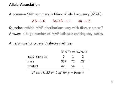
Allele Association

A common SNP summary is Minor Allele Frequency (MAF):

AA → 0 Aa/aA → 1 aa → 2

Question: which MAF distributions vary with disease status?

Answer: a huge number of MAF×disease contingency tables.

An example for type-2 Diabetes mellitus:

MAF: rs6577581

dm2 status 0 1 2

case 357 72 27

control 428 54 1

χ2 stat is 32 on 2 df for p = 9×10−8

22

Dataset has 1000 individuals, 1/2 diabetic, and 7597 SNPs.

Not all SNPs are recorded for all individuals, but most are.

2712 of the tables have cell expectations < 5,

so the χ2 approximation is invalid: drop them.

This leaves us with 4875 χ2-test p-values.

p-values

Frequency

0.0 0.2 0.4 0.6 0.8 1.0

0400

800

Which are significant? We’ll choose a cut-off to control FDR.

23

Controlling the False Discovery Rate

The slope of the FDR-cut line is q/[# of variables].

• significant • not significant

Lots of action!

183 significant tests at FDR of 1e-3. This is (for genetics)

a massive sample, and these SNP locations were targeted.

Much GWAS is not as rich: e.g., Chabris+ Psych Sci 2012.

24

Back to the semiconductors

Semiconductor Signals

p-value

Frequency

0.0 0.2 0.4 0.6 0.8 1.0

020

50

Some are clustered at zero, the rest sprawl out to one.

Which come from null βj = 0? Which are significant?

25

The q = 0.1 line yields 25 ‘significant’ signals.

1 2 5 10 20 50 100 200

1e-06

1e-04

1e-02

1e+00

FDR = 0.1

tests ordered by p-value

p-values

Since the inputs are orthogonal, these are the same

25 most highly correlated-with-y from earlier.

26

The problem with FDR: test dependence

The tests in these examples are plausibly independent:

SNPs are far apart, and PCs are orthogonal.

This seldom holds. Even here: related genes, estimated PCs.

In regression, multicollinearity causes problems: Given two

highly correlated x’s the statistician is unsure which to use.

You then get big p-values and neither variable is significant.

Even with independence, FDR control is often impractical

I Regression p-values are conditional on all other xj’s being

‘in the model’. This is probably a terrible model.

I p-values only exist for p < n, and for p anywhere near to

n you are working with very few degrees of freedom.

But if you are addicted to p-values, its the best you can do.27

Prediction vs Evidence

Hypothesis testing is about evidence: what can we conclude?

Often, you really want to know: what is my best guess?

False Discovery proportions are just one possible model metric.

As an alternative, predictive performance can be easier to

measure and more suited to the application at hand.

This is even true in causal inference:

most of your model components need to predict well for you

to claim structural interpretation for a few chosen variables.

28

Model Building: it is all about prediction.

A recipe for model selection.

1. Find a manageable set of candidate models

(i.e., such that fitting all models is fast).

2. Choose amongst these candidates the one with

best predictive performance on unseen data.

1. is hard. We’ll discuss how this is done...

2. Seems impossible! We need to define some measures of

predictive performance and estimators for those metrics.

29

Metrics of predictive performance

How useful is my model for forecasting unseen data?

Crystal ball: what is the error rate for a given model fitting

routine on new observations from the same DGP as my data?

Bayesian: what is the posterior probability of a given model?

IE, what is the probability that the data came from this model?

These are very closely linked: posteriors are based on

integrated likelihoods, so Bayes is just asking ‘what is the

probability that this model is best for predicting new data?’.

We’ll estimate crystal ball performance with cross validation,

and approximate model probabilities with information criteria.

30

Out-of-sample prediction experiments

We already saw an OOS experiment with the semiconductors.

Implicitly, we were estimating crystal ball R2.

The procedure of using such experiments to do model selection

is called Cross Validation (CV). It follows a basic algorithm:

For k = 1 . . . K,

I Use a subset of nk < n observations to ‘train’ the model.

I Record the error rate for predictions from

this fitted model on the left-out observations.

Error is usually measured in deviance. Alternatives include

MSE, misclass rate, integrated ROC, or error quantiles.

You care about both average and spread of OOS error.

31

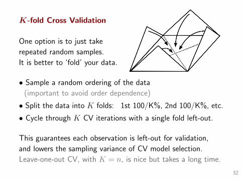
K-fold Cross Validation

One option is to just take

repeated random samples.

It is better to ‘fold’ your data.

• Sample a random ordering of the data

(important to avoid order dependence)

• Split the data into K folds: 1st 100/K%, 2nd 100/K%, etc.

• Cycle through K CV iterations with a single fold left-out.

This guarantees each observation is left-out for validation,

and lowers the sampling variance of CV model selection.

Leave-one-out CV, with K = n, is nice but takes a long time.

32

Problems with Cross Validation

It is time consuming: When estimation is not instant, fitting

K times can become unfeasible even K in 5-10.

It can be unstable: imagine doing CV on many different

samples. There can be huge variability on the model chosen.

It is hard not to cheat: for example, with the FDR cut model

we’ve already used the full n observations to select the 25

strongest variables. It is not surprising they do well OOS.

Still, some form of CV is used in most DM applications.

33

Alternatives to CV: Information Criteria

There are many ‘Information Criteria’ out there: AIC, BIC, ...

These IC are approximations to -log model probabilities.

The lowest IC model has highest posterior probability.

Think Bayes rule for models M1,M2,...MB:

p(Mb|data) =p(data,Mb)

p(data)∝ p(data|Mb)︸ ︷︷ ︸

LHD

p(Mb)︸ ︷︷ ︸prior

The ‘prior’ is your probability that a model is best before you

saw any data. Given Ockham’s razor, p(Mb) should be high

for simple models and low for complicated models.

⇒ exp(-IC) is proportional to model probability.

34

IC and model priors

IC are distinguished by what prior they correspond to.

The two most common are AIC (Akaike’s) and BIC (Baye’s).

These are both proportional to Deviance + k # parameters.

This comes from a Laplace approximation to the integral

− log p(y,Mb) =

∫− log LHD(y|βb)dP(βb)

Akaike uses k = 2 and Bayes uses k = log(n). So BIC uses a

prior that penalizes complicated models more than AIC’s does.

BIC uses a unit-information prior: N(β,− 1

n∂2logLHD∂β2

)AIC’s integrates ∝ exp

[pb2

(log(n)− 1)].

35

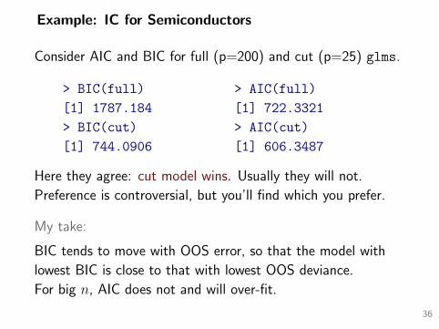
Example: IC for Semiconductors

Consider AIC and BIC for full (p=200) and cut (p=25) glms.

> BIC(full)

[1] 1787.184

> BIC(cut)

[1] 744.0906

> AIC(full)

[1] 722.3321

> AIC(cut)

[1] 606.3487

Here they agree: cut model wins. Usually they will not.

Preference is controversial, but you’ll find which you prefer.

My take:

BIC tends to move with OOS error, so that the model with

lowest BIC is close to that with lowest OOS deviance.

For big n, AIC does not and will over-fit.

36

Forward stepwise regression

Both CV and IC methods require a set of ‘candidate models’.

How do we find a manageable group of good candidates?

Forward stepwise procedures: start from a simple ‘null’ model,

and incrementally update fit to allow slightly more complexity.

Better than backwards methods

I The ‘full’ model can be expensive or tough to fit, while

the null model is usually available in closed form.

I Jitter the data and the full model can change dramatically

(because it is overfit). The null model is always the same.

Stepwise approaches are ‘greedy’: they find the best solution

at each step without thought to global path properties.

Many ML algorithms can be understood in this way.37

Naive stepwise regression

The step() function in R executes a common routine

I Fit all univariate models. Choose that with highest R2

and put that variable – say x(1) – in your model.

I Fit all bivariate models including x(1) (y ∼ β(1)x(1) + βjxj),

and add xj from one with highest R2 to your model.

I Repeat: max R2 by adding one variable to your model.

The algorithm stops when IC is lower for the current

model than for any of the models that add one variable.

Two big problems with this algorithm

Cost: it takes a very long time to fit all these models.

3 min to stop at AIC’s p = 68, 10 sec to stop at BIC’s p = 10.

Stability: sampling variance of the naive routine is very high.38

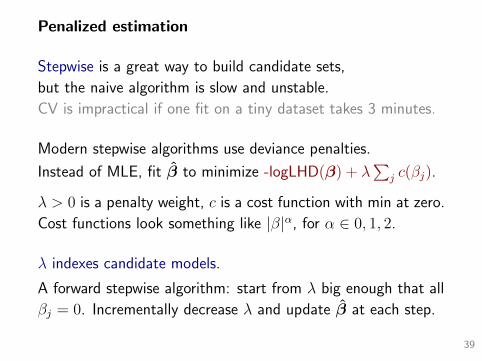
Penalized estimation

Stepwise is a great way to build candidate sets,

but the naive algorithm is slow and unstable.

CV is impractical if one fit on a tiny dataset takes 3 minutes.

Modern stepwise algorithms use deviance penalties.

Instead of MLE, fit β to minimize -logLHD(β) + λ∑

j c(βj).

λ > 0 is a penalty weight, c is a cost function with min at zero.

Cost functions look something like |β|α, for α ∈ 0, 1, 2.

λ indexes candidate models.

A forward stepwise algorithm: start from λ big enough that all

βj = 0. Incrementally decrease λ and update β at each step.

39

Cost functions

Decision theory is based on the idea that choices have costs.

Estimation and hypothesis testing: what are the costs?

Estimation: Deviance is cost of distance from data to model.

Testing: βj = 0 is safe, so it should cost to decide otherwise.

⇒ c should be lowest at β = 0 and we pay more for |β| > 0.

-20 0 20

0200

400

ridge

beta

beta^2

-20 0 20

05

15

lasso

beta

abs(beta)

-20 0 200

2040

60

elastic net

beta

abs(

beta

) + 0

.1 *

bet

a^2

-20 0 20

0.51.52.5

log

beta

log(

1 +

abs(

beta

))

options: ridge β2, lasso |β|, elastic net αβ2 + |β|, log(1 + |β|).

40

Penalization can yield automatic variable selection

-1.0 0.0 1.0 2.0

01

23

4

β

deviance

-1.0 0.0 1.0 2.0

0.0

0.5

1.0

1.5

2.0

βpenalty

-1.0 0.0 1.0 2.0

12

34

56

β

devi

ance

+ p

enal

ty

Anything with an absolute value (e.g., lasso) will do this.

There are MANY penalty options; think of lasso as a baseline.

Important practical point:

Penalization means that scale matters. Most software will

multiply βj by sd(xj) in the cost function to standardize.

41

Cost function properties

Ridge is a James-Stein estimator, with the associated

squared-error-loss optimality for dense signals. It shrinks the

coefficients of correlated variables towards each other.

Concave penalties have oracle properties: βj for ‘true nonzero

coefficients’ converge to MLEs for the true model (Fan+, 200+).

Lasso is a middle ground. It tends to choose a single input

amongst correlated signals but also has a non-diminishing bias.

The lasso does not have Oracle properties.

It gains them if the coefficients are weighted by signal strength

(Zou 2006), and predicts as well as the Oracle if λ is chosen

via CV (Homrighausen + McDonald, 2013).

42

Regularization: depart from optimality to stabilize a system.

Common in engineering: I wouldn’t fly on an optimal plane.

Fitted β for decreasing λ is called a regularization path.

-4 -2 0 2 4

-20123

log penalty

coefficient

201 200 190 129 1 The New Least Squares

For big p, a path to

λ = 0 is faster than a

single full OLS fit.

For the semiconductors

(←) it takes ≈ 4 seconds.

The genius of lasso: β changes smoothly (i.e., very little) when

λ moves, so updating estimates from λt−1 → λt is crazy fast.43

Sound too good to be true? You need to choose λ.

Think of λ as a signal-to-noise filter: like squelch on a radio.

CV: fit training-sample paths and use λ that does best OOS.

-10 -9 -8 -7 -6 -5 -4

24

68

log penalty

bino

mia

l dev

ianc

e

200 195 192 172 129 51 1

Two common rules for ‘best’: min average error, or the largest

λ with mean error no more than 1SE away from the minimum.

44

Any serious software will fit lasso paths and do CV.

-10 -8 -7 -6 -5 -4

-2-1

01

23

Log Lambda

Coefficients

197 188 138 7

-10 -8 -7 -6 -5 -4

0.4

0.8

1.2

1.6

log(Lambda)B

inom

ial D

evia

nce

198 193 182 155 92 11

These plots for semiconductor regression are from glmnet in R.

It’s as simple as fit = cv.glmnet(x,y,family=binomial).

45

IC and the lasso

What are the degrees of freedom for penalized regression?

Think about L0 cost (subset selection): we have p parameters

in a given model, but we’ve looked at all p to choose them.

A fantastic and surprising result about the lasso is that pλ, the

number of nonzero parameters at λ, is an unbiased estimate of

the degrees of freedom (in Stein sense,∑

i cov(yi, yi)/σ2).

See Zou, Hastie, + Tibshrani 2007, plus Efron 2004 on df.

So the BIC for lasso is just deviance + pλ log(n).

This is especially useful when CV takes too long.

(For semiconductors, it agrees with the 1SE rule that p = 1.)

46

Lasso and the Comscore data

Recall web browsing example: y is log spend for 60k online

consumers, and x is the % of visits spent at each of 8k sites.

Lasso path minimizes∑

i12(yi − α− x′β)2 + λ

∑j |βj|.

−10 −8 −6 −4 −2

2.6

2.8

3.0

3.2

3.4

log(Lambda)

Mea

n−S

quar

ed E

rror

●●●●

●●

●●

●●

●●

●●

●●

●●

●●●●●●●●●●●●●●●●●●

●●●

●●

●●

●●

●●

●●

●●

●●

●●

●●

●●

●●

●●

●●

●●●

●●●●

●●●●●

●●●●●●●

●●●●●●●●●●●●●●●●

8216 8005 6843 2488 142 10

●●●●●●●●●●●●●●●●●●●●●●●●●●●●●●●●●●●

●●●●●●●●●●●●●●●●●●●●

●●●●

●●●●

●●●●●

●●●●●●●●

●●●●●●●●●●●●●●●●●●●●●●●

●

−10 −8 −6 −4 −2−

2000

00

2000

0

log(Lambda)

BIC

The BIC mirrors OOS error. This is why practitioners like BIC.47

Comscore regression coefficients

The BIC chooses a model with around 400 nonzero β.

Some of the large absolute values:

shoppingsnap.com onlinevaluepack.com bellagio.com

3.5011219 2.2230610 1.3548940

scratch2cash.com safer-networking.org cashunclaimed.com

-2.0384024 -1.8353769 -1.3052399

tunes4tones.com winecountrygiftbaskets.com marycy.org

-1.5433389 1.4545323 -1.1138126

finestationery.com columbiahouse.com-o01 harryanddavid.com

1.4125547 1.3916690 1.0512341

bizrate.com frontgate.com victoriassecret.com

1.3359164 1.2803210 0.9578552

Note that the most raw dollars were spent on travel sites

(united.com,oribtz.com,hotels.com,...) but these

don’t have the largest coefficients (changes if you scale by sd).

48

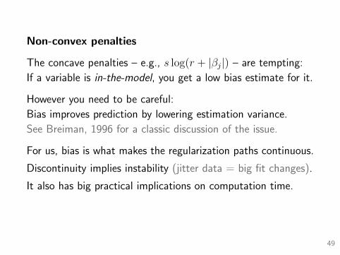
Non-convex penalties

The concave penalties – e.g., s log(r + |βj|) – are tempting:

If a variable is in-the-model, you get a low bias estimate for it.

However you need to be careful:

Bias improves prediction by lowering estimation variance.

See Breiman, 1996 for a classic discussion of the issue.

For us, bias is what makes the regularization paths continuous.

Discontinuity implies instability (jitter data = big fit changes).

It also has big practical implications on computation time.

49

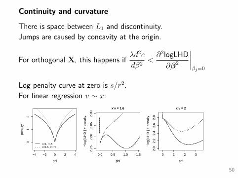
Continuity and curvature

There is space between L1 and discontinuity.

Jumps are caused by concavity at the origin.

For orthogonal X, this happens ifλd2c

dβ2<∂2logLHD

∂β2

∣∣∣∣βj=0

Log penalty curve at zero is s/r2.

For linear regression v ∼ x:

−4 −2 0 2 4

phi

pena

lty

01

2

s=1, r=.5s=1.5, r=.75

0.0 0.5 1.0 1.5

2.75

2.80

2.85

2.90

x'v = 1.6

phi

−lo

g[ L

HD

] +

pen

alty

0 1 2 32.

02.

22.

42.

62.

8

x'v = 2

phi

−lo

g[ L

HD

] +

pen

alty

50

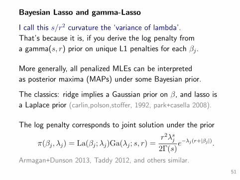
Bayesian Lasso and gamma-Lasso

I call this s/r2 curvature the ‘variance of lambda’.

That’s because it is, if you derive the log penalty from

a gamma(s, r) prior on unique L1 penalties for each βj.

More generally, all penalized MLEs can be interpreted

as posterior maxima (MAPs) under some Bayesian prior.

The classics: ridge implies a Gaussian prior on β, and lasso is

a Laplace prior (carlin,polson,stoffer, 1992, park+casella 2008).

The log penalty corresponds to joint solution under the prior

π(βj, λj) = La(βj;λj)Ga(λj; s, r) =r2λsj2Γ(s)

e−λj(r+|βj |).

Armagan+Dunson 2013, Taddy 2012, and others similar.

51

A useful way to think about penalization

The log penalty is a conjugate prior relaxation of the lasso...

The joint problem is convex, so we get fast globally

convergent estimation under non-convex penalties.

beta

lambda

− objective

beta

lam

bda− objective

Continuity as a function of prior variance is a nice bonus.

Taddy 2013 ‘the gamma lasso’

52

Comscore: time for a single log penalty path fit

1.0

1.5

2.5

4.0

var(lambda)

minutes

subset selection (1/2 hour)

lasso

1e-01 1e+01 1e+03 1e+05 1e+07

Paths are in s/r with s/r2 constant. SS is greedy forward.

The paths here (including SS) all go out to ≈ 5k df.

Full OLS (p ≈ 8k) takes >3 hours on a fast machine.

53

Comscore: path continuity

A quick look at the paths explains our time jumps.

Plotting only the 20 biggest BIC selected β:

120000 140000 160000

-6-4

-20

24

68

deviance

coefficient

5223 595 22 1

var = 1e3

120000 140000 160000

-50

5

deviance

coefficient

5261 385 13 1

var = 1e5

130000 150000 170000

-10

-50

5

deviance

coefficient

5000 2500 1251 1

var = Inf

Algorithm cost explodes with discontinuity.

(var = Inf is subset selection).

54

Factor models: PCA and PCR.

Setting things to zero is just one way to reduce dimension.

Another useful approach is a factor model:

E[x] = v′Φ, where K = dim(v) << dim(x).

Factor regression then just fits E[y] = v′β.

For our semiconductors example, the covariates are

PC directions. So we’ve been doing this all along.

It is best to have both y and x inform estimation of v.

This is ‘supervised’ factorization (also inverse regression).

We’ll just start with the (unsupervised) two stage approach.

55

Factor models: PCA and PCR.

Most common routine is principal component (PC) analysis.

Columns of Φ are eigenvectors of the covariance X′X, so

z = x′Φ is a projection into the associated ortho subspace.

Recall: the actual model is E[x] = v′Φ.

z = x′Φ ∝ v is the projection of x onto our factor space.

If this is confusing you can equate the two without problem.

Full spectral decomposition has ncol(Φ) = min(n,p), but a

factor model uses only the K << p with largest eigenvalues.

56

PCA: projections into latent space

Another way to think about factors, in a 2D example:

PCA equivalent to finding the line that fits through x1 and x2,

and seeing where each observation lands (projects) on the line.

We’ve projected from 2D onto a 1D axis.57

Fitting Principal Components via Least Squares

PCA looks for high-variance projections from multivariate x

(i.e., the long direction) and finds the least squares fit.

-2 -1 0 1 2

-2-1

01

2

x1

x2

PC1PC2

Components are ordered by variance of the fitted projection.

58

A greedy algorithm

Suppose you want to find the first set of factors, v = v1 . . . vn.

We can write our system of equations (for i = 1...n)

E[xi1] = cor(x1, v)vi...

E[xip] = cor(xp, v)vi

The factors v1 are fit to maximize average R2 in this equation.

Next, calculate residuals eij = xij − cor(xj, v1)v1i.

Then find v2 to maximize R2 for these residuals.

This repeats until residuals are all zero (min(p, n) steps).

This is not actually done in practice, but the intuition is nice.59

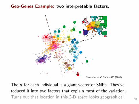
Geo-Genes Example: two interpretable factors.

Novembre et al, Nature 456 (2008)

The x for each individual is a giant vector of SNPs. They’ve

reduced it into two factors that explain most of the variation.

Turns out that location in this 2-D space looks geographical.60

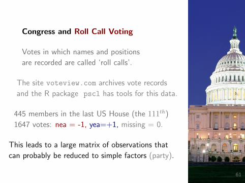
Congress and Roll Call Voting

Votes in which names and positions

are recorded are called ‘roll calls’.

The site voteview.com archives vote records

and the R package pscl has tools for this data.

445 members in the last US House (the 111th)

1647 votes: nea = -1, yea=+1, missing = 0.

This leads to a large matrix of observations that

can probably be reduced to simple factors (party).

61

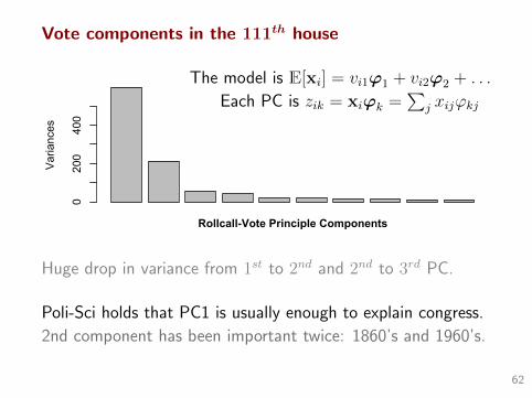
Vote components in the 111th house

The model is E[xi] = vi1ϕ1 + vi2ϕ2 + . . .

Each PC is zik = xiϕk =∑

j xijϕkj

Variances

0200

400

Rollcall-Vote Principle Components

Huge drop in variance from 1st to 2nd and 2nd to 3rd PC.

Poli-Sci holds that PC1 is usually enough to explain congress.

2nd component has been important twice: 1860’s and 1960’s.

62

Top two PC directions in the 111th house

-40 -30 -20 -10 0 10 20

-80

-60

-40

-20

0

PC1

PC2

Republicans in red and Democrats in blue:

I Clear separation on the first principal component.

I The second component looks orthogonal to party.63

Interpreting the principal components

## Far right (very conservative)

> sort(votepc[,1])

BROUN (R GA-10) FLAKE (R AZ-6) HENSARLIN (R TX-5)

-39.3739409 -38.2506713 -37.5870597

## Far left (very liberal)

> sort(votepc[,1], decreasing=TRUE)

EDWARDS (D MD-4) PRICE (D NC-4) MATSUI (D CA-5)

25.2915083 25.1591151 25.1248117

## social issues? immigration? no clear pattern

> sort(votepc[,2])

SOLIS (D CA-32) GILLIBRAND (D NY-20) PELOSI (D CA-8)

-88.31350926 -87.58871687 -86.53585568

STUTZMAN (R IN-3) REED (R NY-29) GRAVES (R GA-9)

-85.59217310 -85.53636319 -76.49658108

PC1 is easy to read, PC2 is ambiguous (is it even meaningful?)

64

High PC1-loading votes are ideological battles.

These tend to have informative voting across party lines.

1st Principle Component Vote-Loadings

Frequency

-0.04 -0.02 0.00 0.02 0.04

0200

400

Afford. Health (amdt.) TARP

A vote for Republican amendments to ‘Affordable Health Care for

America’ strongly indicates a negative PC1 (more conservative), while

a vote for TARP indicates a positive PC1 (more progressive).

65

Look at the largest loadings in ϕ2 to discern an interpretation.

> loadings[order(abs(loadings[,2]), decreasing=TRUE)[1:5],2]

Vote.1146 Vote.658 Vote.1090 Vote.1104 Vote.1149

0.05605862 0.05461947 0.05300806 0.05168382 0.05155729

These votes all correspond to near-unanimous symbolic action.

For example, 429 legislators voted for resolution 1146:

‘Supporting the goals and ideals of a Cold War Veterans Day’

If you didn’t vote for this, you weren’t in the house.

Mystery Solved: the second PC is just attendance!

> sort(rowSums(votes==0), decreasing=TRUE)

SOLIS (D CA-32) GILLIBRAND (D NY-20) REED (R NY-29)

1628 1619 1562

STUTZMAN (R IN-3) PELOSI (D CA-8) GRAVES (R GA-9)

1557 1541 1340

66

PCR: Principal Component Regression

The concept is very simple: instead of regressing onto x, use a

lower dimension set of principal components z as covariates.

This works well for a few reasons:

I PCA reduces dimension, which is always good.

I The PCs are independent: no multicollinearity.

We’ll do exactly this for comscore: just replace E[y|x] = z′β

Factor regressions are especially popular in social science,

because people like to interpret the latent factors.

Be careful though: if you end up needing a large number of

factors it could just be that you don’t have a factor structure.

67

Choosing the number of factors

Without supervision this is tough, but for PCR we can use CV.

1. Regress onto factors 1 through K for a few K, and

choose the model with lowest CV error.

2. Lasso-CV (or other penalty) through all p factors.

The standard routine is to do ‘1’, but this is unnecessary given

our alternative ways to build regularized candidate sets.

NB: unfortunately the approximations that go into BIC don’t

work with factor models (K factor parameters in addition to

the coefficients). It often works, but will break for large K.

(Roeder + Wasserman 1997 for BIC justification in such context)

68

Comscore PC factors

●●

●

●●● ●●

●●

● ●●●●

●●

● ●●

●● ●● ●●

●

●●

●●●●

●●

●

●● ● ● ●●●●●

●

●

●

●

●

●

●●

●●● ●●●●●●

●

●●●

●

●●

●● ●

●●●

●

●●

●

●●●

●

●●●

●● ●● ●

●●

●●●●

●●

●●

●

●●●●●

●●

●

●

●

●●●●

●●

●

●●● ●●●● ●

●

●

●

●●

●

●●

●●●●●

●

●●● ●

●

●● ●

● ●●●

●

●●

●

●●

●●●●

●●

●

●

●

●

●●

●●

●

●

●●●

●

●

●

●●

●

● ●●●●

●

● ●●●●

●●●

●

●●

●

●

●

●●●●

●

●●

●●

●●●●●

●

●●

● ● ●●

●

●

−20 −15 −10 −5 0 5 10

−50

−30

−10

0

pc1

pc2

●● ●●●

●●

●

●

●

●

●●

●

●

● ●

●

●●

●

●●●●●

●

●●

●●●

●●●

●

●

●●●●●

●●

●

● ●●●

●

●●

●●

●● ●

●

●●

●●●

●●●●

●●

●

●

●● ●●

●

●

●

●

●●

●

● ●●

● ●●●

●

●

●

●●●●

●

●●

●

● ●

●●

● ●

●●

●

●

●●

●

●●

●

●

●

●

●

●● ●●

●

●

●

●● ●●●●

●● ●

●

●

●●

●●

●●●

● ●●●●●

●●

●

●

●

● ●

●

●

●●

●

●

●

●

●

●●●●

●

●

●

●

●

●

●

●

●

●

●●●

●●●

●

●

●● ●

●●●

●

●●

●

●

●

●

●●●● ●●●

●●

●● ●●

●

●●●

●

●

●●●●●●

−10 0 10 20 30

−20

010

2030

pc3

pc4

machines sized by log consumption

PC1 has big loadings on ad trackers and providers

(atdmt.com, zedo.com, googlesyndication.com),

PC2 is all just big negatives on porn (I’ll shield you), ...

69

Mixing methods: CV, penalization, and PCs.

How to choose the number of factors?

We can do lasso-CV for y on z.

5 6 7 8 9

2.7

2.8

2.9

3.0

log penalty

gaus

sian

dev

ianc

e

●●●●●●●

●●

●●

●●

●●

●●

●●

●●

●●

●●

●●

●●●●●●●●●●●●●●●●●●●●●●●●●●●●●●●●●●●●●●●●●●●●●●●●●●●●●●●●●●●●●●●●●●●●●●●●●

95.9 84.7 47.2 15 1

5 6 7 8 9

−0.

050.

000.

05log penalty

coef

ficie

nt

95.9 84.7 47.2 15 1

Even though we’ve done variable (factor) selection,

every model for λ < λ0 is dense: β1zik = β1ϕjkxij.70

Large absolute value coefficients on scaled xj/sjlillianvernon.com victoriassecret.com liveperson.net

0.010568003 0.010467798 0.010457976

neimanmarcus.com revresda.com oldnavy.com

0.010402899 0.010313770 0.010199234

homedecorators.com kohls.com richfx.com

0.009989661 0.009960027 0.009864902

And on raw xjthestationerystudio.com diamond.com ordermedia.com

0.7397097 0.7378156 0.7320079

raffaello-network.com visitlasvegas.com spafinder.com

0.7279747 0.7247268 0.7170530

onewayfurniture.com finestationery.com mandalaybay.com

0.7136429 0.7064830 0.6880314

In the PC regression, biggest β were on factors 18, 35, 22.

Pretty deep: is factorization useful?

Nope: compare to original lasso OOS deviance.71

Alternative Factor Models

When > 99% of your data are zero, assuming they are

independent and normal (i.e. using least squares) can break.

These are the cases where functional form actually matters.

Recall our factorization E[xi] = ϕ1vi1 + . . .ϕKviK .

The count-data version is a topic model

xi ∼ MN(vi1θ1 + . . .+ viKθK ,m)

Topics∑p

j=1 θkj = 1 and weights∑K

k=1 vik = 1,

so an observation (x) is drawn from a multinomial with

probabilities that are a mixture of topics θ1 . . .θK .

Also ‘LDA’: latent Dirichlet allocation Blei,Ng,Jordan 2003.

72

Topic Models: factors for count data

They really can lead to better factorizations (e.g. Taddy 2013

techno), but because of the nonlinearity they take longer to fit.

Taddy 2012 describes fast numeric approximation

to the model probabilities∫

LHD(X|Θ,V)dP(Θ,V).

Hoffman, Blei, Wang, Paisley 2013 use stochastic gradient

approximation to just fit the model faster (enough for CV).

There is a big literature on topic model approximation...

Generally when working with topic models and big data you

give up precision in exchange for a better functional form.

73

Topic modeling Comscore

Instead of looking at proportion of time spent on each site,

we’ll use raw machine-domain counts (# of visits) as x.

Since it takes so long (a common refrain) I just fit for K=25.

> tpc <- topics(x, K=25)

> summary(tpc)

Top phrases by topic-over-null term lift (and usage %):

[2] meegos.com, footprint.net, passport.net, passport.com

[3] regionsnet.com, gwu.edu, drexel.edu, ku.edu, regions.com

[4] catcha10.com, treborwear.com, whateverlife.com, webgavel.com

[5] waol.exe, acsd.exe, aolacsd.exe, aol.com-o07, aoltpspd.exe

[8] worldofwarcraft.com, mininova.org, beboframe.com, runescape.com

[9] drudgereport.com, eproof.com, mercuras.com, breitbart.com

[10] eimg.net, paviliondownload.com, wachoviabillpay.com, marykayintouch.com

[11] freeslots.com, iwon.com-o04, jigzone.com, luckysurf.com

....

74

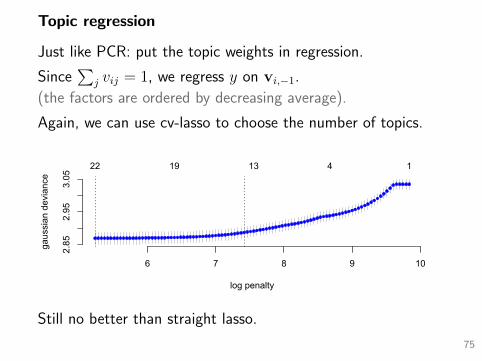
Topic regression

Just like PCR: put the topic weights in regression.

Since∑

j vij = 1, we regress y on vi,−1.

(the factors are ordered by decreasing average).

Again, we can use cv-lasso to choose the number of topics.

6 7 8 9 10

2.85

2.95

3.05

log penalty

gaus

sian

dev

ianc

e

22 19 13 4 1

Still no better than straight lasso.

75

In conclusion, the Recipe:

Build a forward stepwise path of candidate regularized models,

then select the best via CV (or BIC if you are pressed on time).

If you think you have factor structure, try fitting that first.

There is a ton more to ‘data science’.

I Supervised factor models and inverse regression:

model x|y for efficient ‘weak signal’ factorization.

I Trees and forests: decision trees, and techniques for

averaging many possible trees: bagging and MCMC.

I More generally: model averaging and ensemble methods;

e.g. predicting y as a weighted average across different λ.

I MapReduce and distributed algorithms...

Have fun with it!76