Multinomial Inverse Regression for Text Analysis

Matt Taddytaddy@chicagobooth.edu

The University of Chicago Booth School of Business

ABSTRACT: Text data, including speeches, stories, and other document forms, are often connected tosentiment variables that are of interest for research in marketing, economics, and elsewhere. It is alsovery high dimensional and difficult to incorporate into statistical analyses. This article introduces astraightforward framework of sentiment-sufficient dimension reduction for text data. Multinomial in-verse regression is introduced as a general tool for simplifying predictor sets that can be representedas draws from a multinomial distribution, and we show that logistic regression of phrase counts ontodocument annotations can be used to obtain low dimension document representations that are rich insentiment information. To facilitate this modeling, a novel estimation technique is developed for multi-nomial logistic regression with very high-dimension response. In particular, independent Laplace priorswith unknown variance are assigned to each regression coefficient, and we detail an efficient routine formaximization of the joint posterior over coefficients and their prior scale. This ‘gamma-lasso’ schemeyields stable and effective estimation for general high-dimension logistic regression, and we argue thatit will be superior to current methods in many settings. Guidelines for prior specification are provided,algorithm convergence is detailed, and estimator properties are outlined from the perspective of theliterature on non-concave likelihood penalization. Related work on sentiment analysis from statistics,econometrics, and machine learning is surveyed and connected. Finally, the methods are applied in twodetailed examples and we provide out-of-sample prediction studies to illustrate their effectiveness.

Taddy is an Associate Professor of Econometrics and Statistics and Neubauer Family Faculty Fellow at the Uni-

versity of Chicago Booth School of Business, and this work was partially supported by the IBM Corporation

Faculty Research Fund at Chicago. The author thanks Jesse Shapiro, Matthew Gentzkow, David Blei, Che-Lin

Su, Christian Hansen, Robert Gramacy, Nicholas Polson, and anonymous reviewers for much helpful discussion.

arX

iv:1

012.

2098

v7 [

stat

.ME

] 8

Aug

201

3

1 Introduction

This article investigates the relationship between text data – product reviews, political speech,

financial news, or a personal blog post – and variables that are believed to influence its com-

position – product quality ratings, political affiliation, stock price, or mood polarity. Such

language-motivating observable variables, generically termed sentiment in the context of this

article, are often the main object of interest for text mining applications. When, as is typical,

large amounts of text are available but only a small subset of documents are annotated with

known sentiment, this relationship yields the powerful potential for text to act as a stand-in for

related quantities of primary interest. On the other hand, language data dimension (i.e., vocab-

ulary size) is both very large and tends to increase with the amount of observed text, making the

data difficult to incorporate into statistical analyses. Our goal is to introduce a straightforward

framework of sentiment-preserving dimension reduction for text data.

As detailed in Section 2.1, a common statistical treatment of text views each document as

an exchangeable collection of phrase tokens. In machine learning, these tokens are usually just

words (e.g., tax, pizza) obtained after stemming for related roots (e.g., taxation, taxing, and

taxes all become tax), but richer tokenizations are also possible: for example, we find it useful

to track common n-gram word combinations (e.g. bigrams pay tax or cheese pizza and trigrams

such as too much tax). Under a given tokenization each document is represented as xi =

[xi1, . . . , xip]′, a sparse vector of counts for each of p tokens in the vocabulary. These token

counts, and the associated frequencies fi = xi/mi wheremi =∑p

j=1 xij , are then the basic data

units for statistical text analysis. In particular, the multinomial distribution for xi implied by an

assumption of token-exchangeability can serve as the basis for efficient dimension reduction.

Consider n documents that are each annotated with a single sentiment variable, yi (e.g.,

restaurant reviews accompanied by a one to five star rating). A naive approach to text-sentiment

prediction would be to fit a generic regression for yi|xi. However, given the very high dimen-

sion of text-counts (with p in the thousands or tens of thousands), one cannot efficiently estimate

this conditional distribution without also taking steps to simplify xi. We propose an inverse re-

gression (IR) approach, wherein the inverse conditional distribution for text given sentiment is

used to obtain low dimensional document scores that preserve information relevant to yi.

As an introductory example, consider the text-sentiment contingency table built by col-

2

lapsing token counts as xy =∑

i:yi=yxi for each y ∈ Y , the support of an ordered discrete

sentiment variable. A basic multinomial inverse regression (MNIR) model is then

xy ∼ MN(qy,my) with qyj =exp[αj + yϕj]∑pl=1 exp[αl + yϕl]

, for j = 1, . . . , p, y ∈ Y (1)

where each MN is a p-dimensional multinomial distribution with size my =∑

i:yi=ymi and

probabilities qy = [qy1, . . . , qyp]′ that are a linear function of y through a logistic link. Under

conditions detailed in Section 3, the sufficient reduction (SR) score for fi = xi/mi is then

zi = ϕ′fi ⇒ yi ⊥⊥ xi,mi | zi. (2)

Hence, given this SR projection, full xi is ignored and modeling the text-sentiment relation-

ship becomes a univariate regression problem. This article’s examples include linear, E[yi] =

β0+β1zi, quadratic,E[yi] = β0+β1zi+β2z2i , and logistic, p(yi < a) = (1 + exp[β0 + β1zi])

−1,

forms for this forward regression, and SR scores should be straightforward to incorporate into

alternative regression models or structural equation systems. The procedure rests upon assump-

tions that allow for summary tables wherein the text-sentiment relationship of interest can be

modeled as a logistic multinomial, but when such assumptions are plausible, as we find com-

mon in text analysis, they introduce information that should yield significant efficiency gains.

In estimating models of the type in (1), which involve many thousands of parameters, we

propose use of fat-tailed and sparsity-inducing independent Laplace priors for each coefficient

ϕj . To account for uncertainty about the appropriate level of variable-specific regularization,

each Laplace rate parameter λj is left unknown with a gamma hyperprior. Thus, for example,

π(ϕj, λj) =λj2e−λj |ϕj | r

s

Γ(s)λs−1j e−rλj , s, r, λj > 0, (3)

independent for each j under a Ga(s, r) hyperprior specification. This departure from the usual

shared-λ model is motivated in Section 3.3.

Fitting MNIR models is tough for reasons beyond the usual difficulties of high dimension

regression – simply evaluating the large-response likelihood is expensive due to the normal-

ization in calculating each qi. As surveyed in Section 4, available cross-validation (e.g., via

3

solution paths) and fully Bayesian (i.e., through Monte-Carlo marginalization) methods for es-

timating ϕj under unknown λj are prohibitively expensive. A novel algorithm is proposed for

finding the joint posterior maximum (MAP) estimate of both coefficients and their prior scale.

The problem is reduced to log likelihood maximization for ϕ with a non-concave penalty, and

it can be solved relatively quickly through coordinate descent. For example, given the prior in

(3), the log likelihood implied by (1) is maximized subject to (i.e., minus) cost constraints

c(ϕj) = s log(1 + |ϕj|/r) (4)

for each coefficient. This provides a powerful new estimation framework, which we term the

gamma-lasso. The approach is very computationally efficient, yielding robust SR scores in

less than a second for documents with thousands of unique tokens. Indeed, although a full

comparison is beyond the scope of this paper, we find that the proposed algorithm can also be

far superior to current techniques for high-dimensional logistic regression in the more common

large-predictor (rather than large-response) setting.

This article thus includes two main methodological contributions. First, Section 3 intro-

duces multinomial inverse regression as an IR procedure for predictor sets that can be rep-

resented as draws from a multinomial, and details its application to text-sentiment analysis.

This includes full model specification and general sufficiency results, guidelines on how text

data should be handled to satisfy the MNIR model assumptions, and our independent gamma-

Laplace prior specification. Second, Section 4 develops a novel approach to estimation in very

high dimensional logistic regression. This includes details of coordinate descent for joint MAP

estimation of coefficients and their unknown variance, and an outline of estimator properties

from the perspective of the literature on non- concave likelihood penalization. As background,

Section 2 briefly surveys the literature on text mining and sentiment analysis, and on dimension

reduction and inverse regression.

The following section describes language pre-processing and introduces two datasets that

are used throughout to motivate and illustrate our methods. Performance comparison and de-

tailed results for these examples are then presented in Section 5. Both example datasets, along

with all implemented methodology, are available in the textir package for R.

4

1.1 Data processing and examples

Text is usually initially cleaned according to some standard information retrieval criteria, and

we refer the reader to Jurafsky and Martin (2009) for an overview. In this article, we simply

remove a limited set of stop words (e.g., and or but) and punctuation, convert to lowercase,

and strip suffixes from roots according to the Porter stemmer (Porter, 1980). The main data

preparation step is then to parse clean text into informative language tokens; as mentioned in

the introduction, counts for these tokens are the starting point for statistical analysis. Most

commonly (see, e.g., Srivastava and Sahami, 2009) the tokens are just words, such that each

document is treated as a vector of word-counts. This is referred to as the bag-of-words rep-

resentation, since these counts are summary statistics for language generated by exchangeable

draws from a multinomial ‘bag’ of word options.

Despite its apparent limitations, the token-count framework can be made quite flexible

through more sophisticated tokenization. For example, in the N -gram language model words

are drawn from a Markov chain of order N (see, e.g., Jurafsky and Martin, 2009). A document

is then summarized by its length-N word sequences, or N -gram tokens, as these are sufficient

for the underlying Markov transition probabilities. Our general practice is to count common

unigram, bigram, and trigram tokens (i.e., words and 2-3 word phrases). Another powerful

technique is to use domain-specific knowledge to parse for phrases that are meaningful in the

context of a specific field. Talley and O’Kane (2011) present one such approach for tokeniza-

tion of legal agreements; for example, they use any conjugation of the word act in proximity of

God to identify a common Act of God class of carve-out provisions. Finally, work such as that

of Poon and Domingos (2009) seeks to parse language according to semantic equivalence.

Thus while we focus on token-count data, different language models are able to influence

analysis through tokenization rules. And although separation of parsing from statistical mod-

eling limits our ability to quantify uncertainty, it has the appealing effect of allowing text data

from various sources and formats to all be analyzed within a multinomial likelihood framework.

1.1.1 Ideology in political speeches

This example originally appears in Gentzkow and Shapiro (GS; 2010) and considers text of the

109th (2005-2006) Congressional Record. For each of the 529 members of the United States

5

House and Senate, GS record usage of phrases in a list of 1000 bigrams and trigrams. Each

document corresponds to a single person. The sentiment of interest is political partisanship,

where party affiliation (Republican, Democrat, or Independent) provides a simple indicator

and a higher-fidelity measure is calculated as the two-party vote-share from each speaker’s

constituency (congressional district for representatives; state for senators) obtained by George

W. Bush in the 2004 presidential election. Note that token vocabulary in this example is influ-

enced by sentiment: GS built contingency tables for bigram and trigram usage by party, and

kept the top 1000 ‘most partisan’ phrases according to ranking of their Pearson χ2-test statistic.

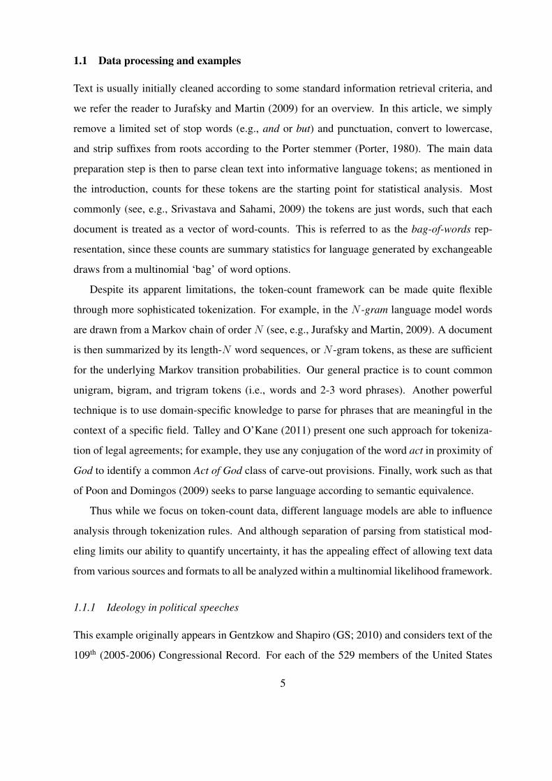
Define phrase frequency lift for a given group as fjG/fj , where fjG is mean frequency for

phrase j in group G and fj =∑n

i=1 fij/n is the average across all documents. The following

tables show top-five lift phrases used at least once by each party.

DEMOCRATIC FREQUENCY LIFT

congressional.hispanic.caucu 2.163medicaid.cut 2.154

clean.drinking.water 2.154earth.day 2.152

tax.cut.benefit 2.149

REPUBLICAN FREQUENCY LIFT

ayman.al.zawahiri 1.850america.blood.cent 1.849

million.budget.request 1.847million.illegal.alien 1.846

temporary.worker.program 1.845

1.1.2 On-line restaurant reviews

This dataset, which originally appears in the topic analysis of Maua and Cozman (2009), con-

tains 6260 user-submitted restaurant reviews (90 word average) from www.we8there.com.

The reviews are accompanied by a five-star rating on four specific aspects of quality – food,

service, value, and atmosphere – as well as the overall experience. After tokenizing the text

into bigrams (based on a belief that modifiers such as very or small would be useful here), we

discard phrases that appear in less than ten reviews and documents which do not use any of the

remaining phrases. This leaves a dataset of 6147 review counts for a token vocabulary of 2978

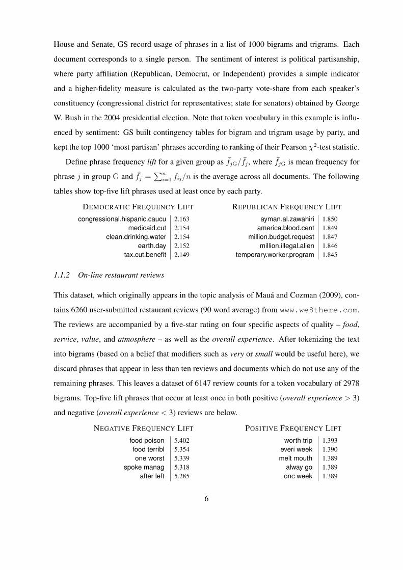
bigrams. Top-five lift phrases that occur at least once in both positive (overall experience > 3)

and negative (overall experience < 3) reviews are below.

NEGATIVE FREQUENCY LIFT

food poison 5.402food terribl 5.354one worst 5.339

spoke manag 5.318after left 5.285

POSITIVE FREQUENCY LIFT

worth trip 1.393everi week 1.390melt mouth 1.389

alway go 1.389onc week 1.389

6

2 Background

This section briefly reviews the relevant literatures on sentiment analysis and inverse regression.

Additional background is in the appendices and material specific to estimation is in Section 4.

2.1 Analysis of sentiment in text

As already outlined, we use sentiment to refer to any variables related to document composition.

Although broader than its common ‘opinion polarity’ usage, this definition as ‘sensible quality’

fits our need to refer to the variety of quantities that may be correlated with text.

Much of existing work on sentiment analysis uses word frequencies as predictors in generic

regression and classification algorithms, including support vector machines, principle compo-

nents (PC) regression, neural networks, and penalized least-squares. Examples from this ma-

chine learning literature can be found in the survey by Pang and Lee (2008) and in the collection

from Srivastava and Sahami (2009). In the social sciences, research on ideology in political text

includes both generic classifiers (e.g., Yu et al., 2008) and analysis of contingency tables for

individual terms (e.g., Laver et al., 2003) (machine learning researchers, such as Thomas et al.,

2006, have also made contributions in this area). In economics, particularly finance, it is more

common to rely on weighted counts for pre-defined lists of terms with positive or negative tone;

examples of this approach include Tetlock (2007) and Loughran and McDonald (2011) (again,

machine learners such as Bollen et al., 2011, have also studied prediction for finance).

These approaches all have drawbacks: generic regression does nothing to leverage the par-

ticulars of text data, independent analysis of many contingency tables leads to multiple-testing

issues, and pre-defined word lists are subjective and unreliable. A more promising strategy is

to use text-specific dimension reduction based upon the multinomial implied by exchangeabil-

ity of token-counts. For example, a topic model treats documents as drawn from a multino-

mial distribution with probabilities arising as a weighted combination of ‘topic’ factors. Thus

xi ∼ MN(ωi1θ1 + . . .+ ωiKθK ,mi), where topics θk = [θk1 · · · θkp]′ and weights ωi are prob-

ability vectors. This framework, also known as latent Dirichlet allocation (LDA), has been

widely used in text analysis since its introduction by Blei et al. (2003).

The low dimensional topic-weight representation (i.e., ωi) serves as a basis for sentiment

7

analysis in the original Blei et al. article, and has been used in this way by many since. The

approach is especially popular in political science, where work such as that of Grimmer (2010)

and Quinn et al. (2010) investigates political interpretation of latent topics (these authors re-

strict ωik ∈ {0, 1} such that each document is drawn from a single topic). Recently, Blei and

McAuliffe (2007) have introduced supervised LDA (sLDA) for joint modeling of text and sen-

timent. In particular, they augment topic model with a forward regression yi = f(ωi), such

that token counts and sentiment are connected through shared topic-weight factors.

Finally, our investigation was originally motivated by a desire to build a model-based ver-

sion of the specific slant indices proposed by Gentzkow and Shapiro (2010), which are part of

a general political science literature on quantifying partisanship through weighted-term indices

(e.g., Laver et al., 2003). Appendix A.1 shows that the GS indices can be written as summation

of phrase frequencies loaded by their correlation with measured partisanship (e.g., vote-share),

such that slant is equivalent to first-order partial least-squares (PLS; Wold, 1975).

2.2 Inverse regression and sufficient reduction

This article is based on a notion that, given the high dimension of text data, it is not possible to

efficiently estimate conditional response y|x without finding a way to simplify x. The same idea

motivates many of the techniques surveyed above, including LDA and sLDA, PLS/slant, and

PC regression. A framework to unify techniques for dimension reduction in regression can be

found in Cook’s 2007 overview of inverse regression, wherein inference about the multivariate

conditional distribution x|y is used to build low dimension summaries for x.

Suppose that vi is a K-vector of response factors through which xi depends on yi (i.e., vi

is a possibly random function of yi). Then Cook’s linear IR formulation has xi = Φvi + εi,

where Φ = [ϕ1 · · ·ϕK ] is a p ×K matrix of inverse regression coefficients and εi is p-vector

of error terms. Under certain conditions on var(εi), detailed by Cook, the projection zi = Φ′xi

provides a sufficient reduction (SR) such that yi is independent of xi given zi. As this implies

p(xi|Φ′xi, yi) = p(xi|Φ′xi), SR corresponds to the classical definition of sufficiency for ‘data’

xi and ‘parameter’ yi, but is conditional on unknown Φ that must be estimated in practice.

When such estimation is feasible, the reduction of dimension from p to K should make these

SR projections easier to work with than the original predictors.

8

Many approaches to dimension reduction can be understood in context of this linear IR

model: PC directions arise as SR projections for the maximum likelihood solution when vi is

unspecified (see, e.g., Cook, 2007) and, following our discussion in A.1, the first PLS direction

is the SR projection for least-squares fit when vi = yi. A closely related framework is that of

factor analysis, wherein one seeks to estimate vi directly rather than project xi into its lower

dimensional space. By augmenting estimation with a forward model for yi|vi researchers are

able to build supervised factor models; see, e.g., West (2003).

The innovation of inverse regression, from Cook’s 2007 paper and in earlier work including

Li (1991) and Bura and Cook (2001), is to investigate the SR projections that result from ex-

plicit specification for vi as a function of yi. Cook’s principle fitted components are derived for

a variety of functional expansions of yi, Li et al. (2007) interprets PLS within an IR framework,

and the sliced inverse regression of Li (1991) defines vi as a step-function expansion of yi.

Since in each case the vi are conditioned upon, these IR models are more restrictive than the

random joint forward-inverse specification of supervised factor models. But if the IR model

assumptions are satisfied then its parsimony should lead to more efficient inference.

Instead of a linear equation, dimension reduction for text data is based on multinomial

models. Following the topic model factor specification, LDA is akin to PC analysis for multi-

nomials and sLDA is the corresponding supervised factor model. However, existing work on

non-Gaussian inverse regression relies on conditional independence; for example, Cook and Li

(2009) use single-parameter exponential families to model each xij|vi. To our knowledge, no-

one has investigated SR projections based on the multinomial predictor distributions that arise

naturally for text data. Hence, we seek to build a multinomial inverse regression framework.

3 Modeling

The subject-specific multinomial inverse regression model has, for i = 1, . . . , n:

xi ∼ MN(qi,mi) with qij =eηij∑pl=1 e

ηil, j = 1, . . . , p, where ηij = αj + uij + v′iϕj. (5)

This generalizes (1) with the introduction of K-dimensional response factors vi and subject

effects ui = [ui1 · · ·uip]′. Section 3.1 derives sufficient reduction results for projections zimi =

9

Φ′xi, where Φ′ = [ϕ1, · · ·ϕp]. Section 3.2 then describes application of these results in text

analysis and outlines situations where (5) can be replaced with a collapsed model as in (1).

Finally, 3.3 presents prior specification for these very high dimensional regressions.

3.1 Sufficient reduction in multinomial inverse regression

This section establishes classical sufficiency-for-y (conditional on IR parameters) for projec-

tions derived from the model in (5). The main result follows, due to use of a logit link on ηi =

[ηi1 · · · ηip]′, from factorization of the multinomial’s natural exponential family parametrization.

PROPOSITION 3.1. Under the model in (5), conditional on mi and ui

yi ⊥⊥ xi | vi ⇒ yi ⊥⊥ xi | Φ′xi.

Proof. Setting αij = αj + uij and suppressing i, the likelihood is(mx

)exp [x′η − A(η)] =(

mx

)ex

′α exp [(x′Φ)v − A(η)] = h(x)g(Φ′x,v), where A(η) = m log[∑p

j=1 eηj

]. Hence, the

usual sufficiency factorization (e.g., Schervish, 1995, 2.21) implies p(x|Φ′x,v) = p(x|Φ′x),

and v is independent of x given Φ′x. Finally, p(y|x,Φ′x) =∫vp(y|v)dP(v|Φ′x) = p(y|Φ′x).

Second, it is standard in text analysis to control for document size by regressing yi onto fre-

quencies rather than counts. Fortunately, our sufficient reductions survive this transformation.

PROPOSITION 3.2. If yi ⊥⊥ xi | Φ′xi,mi and p(y | xi) = p(yi | fi), then yi ⊥⊥ xi | zi = Φ′fi.

Proof. We have that each of f and [Φ′f ,m] are sufficient for y in p(x|y) = MN(q,m)p(m|y).

Under conditions of Lehmann and Sheffe (1950, 6.3), there exists a minimal sufficient statistic

T (x) and functions g and g such that g(f) = T (x) = g(Φ′f ,m). Having g vary with m, while

g(f) does not, implies that the map Φ′f has introduced such dependence. But since m cannot

be recovered from f , this must be false. Thus g = g(Φ′f), and z = Φ′f is sufficient for y.

3.2 MNIR for sentiment in text: collapsibility and random effects

For text-sentiment response factor specification, we focus on untransformed vi = yi and dis-

cretized vi = step(yi) along with their analogues for multivariate sentiment. The former is

appropriate for categorical sentiment (e.g., political party, or 1-5 star rating) and, for reasons

10

discussed below, the latter is used with continuous sentiment (e.g., vote-share is rounded to the

nearest whole percentage, and in general one can bin and average y by quantiles). Regardless,

our methods apply under generic v(yi) including, e.g., the expansions of Cook (2007).

Given this setting of discrete vi, MNIR estimation can often be based on the collapsed

counts that arise by aggregating within factor level combinations. For example, since sums

of multinomials with equal probabilities are also multinomial, given shared intercepts (i.e.,

uij = 0) and writing the support of vi as V , the likelihood for the model in (5) is exactly the

same as that from, for v ∈ V with xv =∑

i:vi=v xi and mv =∑

i:vi=vmi,

xv ∼ MN(qv,mv), where qvj =eηvj∑pl=1 e

ηvland ηvj = αj + vϕj. (6)

Since pooling documents in this way leaves only as many ‘observations’ as there are levels in

the support of vi, it can lead to dramatically less expensive estimation.

Under the marginal model of (6), Φ is the population average effect of v on x. One needs

to be careful in when and how estimates from this model are used in SR projection, since condi-

tional document-level validity of these results is subject to the usual collapsibility requirements

for analysis of categorical data (e.g., Bishop et al., 1975). In particular, omitted variables must

be conditionally independent of xi given vi; this can usually be assumed for sentiment-related

variables (e.g., a congress person’s voting record is ignored given their party and vote-share).

Covariates that act on xi independent of vi should be included in MNIR, as part of the equation

for subject effects ui (e.g., although it is not considered in this article, it might be best to condi-

tion on geography when regressing political speech onto partisanship). The sufficient reduction

result of (3.1) is then conditional on these sentiment-independent variables, such that they (or

their SR projection) may need to be used as inputs in forward regression.

It is often unreasonable to assume that known factors account for all variation across docu-

ments, and treating the ui of (5) as random effects independent of vi provides a mechanism for

explaining such heterogeneity and understanding its effect on estimation. Omitting ui ⊥⊥ vi

tends to yield estimated Φ that is attenuated from its correct document-specific analogue (Gail

et al., 1984), although the population-average estimators can be reliable in some settings; for

example, Zeger et al. (1985) show consistency for the stationary distribution effect of covari-

11

ates when the ui encode temporal dependence (such as that between consecutive tokens in an

N -gram text model). When their influence is considered negligible, it is common to simply

ignore the random effects in estimation. In this article we also consider modeling euij as in-

dependent gamma random variables, and use this to motivate a prior in 3.3 for the marginal

random effects in a collapsed table. Another option would be to incorporate latent topics into

MNIR and parametrize ui through a linear factor model; this is especially appealing since SR

projections onto estimated factor scores could then be used in forward regression.

This last point – on random effects and forward regression – is important: when Φ is

estimated with random effects, Section 3.1 only establishes sufficiency of zi conditional on

ui. Marginal sufficiency would follow from p(vi|ui,Φ′xi) = p(vi|Φ′xi), which for ui ⊥⊥ vi

requires ui ⊥⊥ Φ′xi. Thus, information about vi from this marginal dependence is lost when

(as is usually necessary) ui is omitted in regression of vi onto zi. Section 5 shows that random

effects in MNIR can be beneficial even if they are then ignored in forward regression. However,

SR projection onto parametric representations of ui is an open research interest.

It is clear that there are many relevant issues to consider when assessing an MNIR model,

and it is helpful to have our sentiment regression problem placed within the well studied frame-

work of contingency table analysis (e.g., Agresti, 2002, is a general reference). Ongoing work

centers on inference according to specific dependence structures or random effect parametriza-

tions. However, as illustrated in Section 5, even very simple MNIR models – measuring popu-

lation average effects – allow SR projections that are powerful tools for forward prediction.

3.3 Prior specification

To complete the MNIR model, we provide prior distributions for the intercepts α, loadings Φ,

and possible random effects U = [uv1 · · ·uvd]′, where d is the number of points in V .

First, each phrase intercept is assigned an independent standard normal prior, αj ∼ N(0, 1).

This serves to identify the logistic multinomial model, such that there is no need to spec-

ify a null category, and we have found it diffuse enough to accomodate category frequencies

in a variety of text and non-text examples. Second, we propose independent Laplace pri-

ors for each ϕjk, with coefficient-specific precision (or ‘penalty’) parameters λjk, such that

π(ϕjk) = λjk/2 exp(−λjk|ϕjk|) for j = 1 . . . p and k = 1 . . . K. The implied prior stan-

12

dard deviation for ϕjk is√

2/λjk. Each λjk is then assigned a conjugate gamma hyperprior

Ga(λjk; s, r) = rs/Γ(s)λs−1jk e−rλjk , yielding the joint gamma-Laplace prior introduced in (3).

Hyperprior shape, s, and rate, r, imply expectation s/r and variance s/r2 for each λjk.

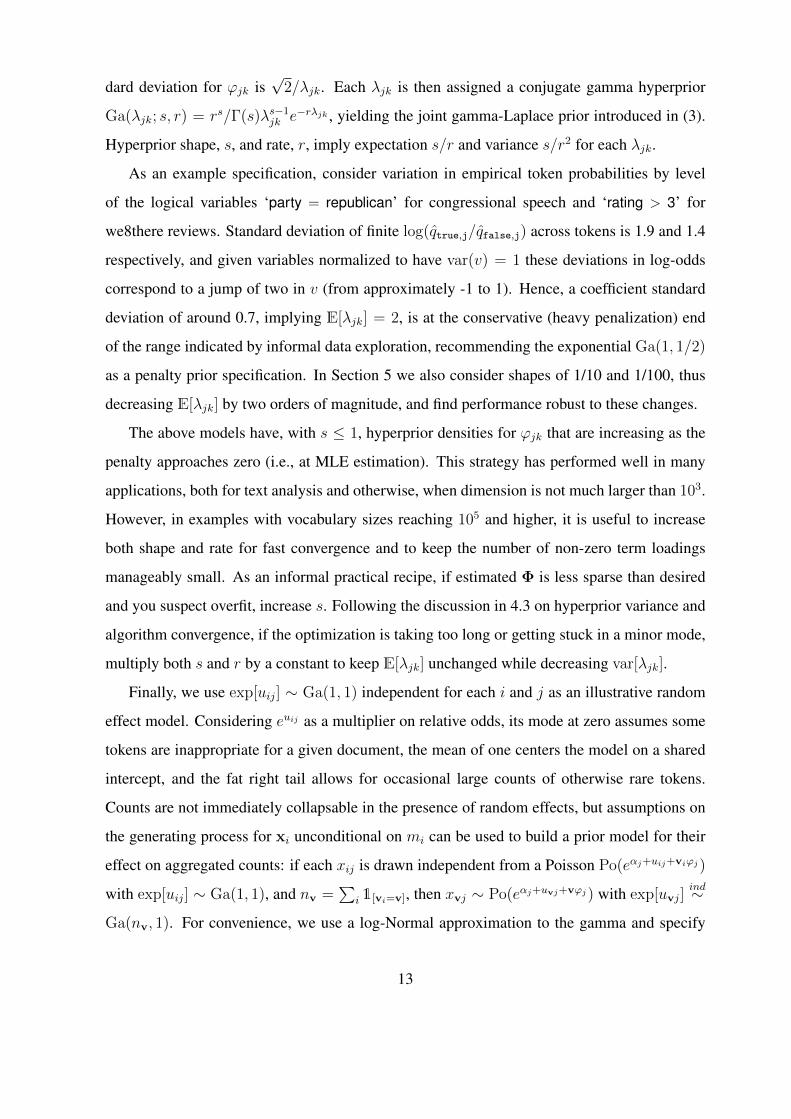
As an example specification, consider variation in empirical token probabilities by level

of the logical variables ‘party = republican’ for congressional speech and ‘rating > 3’ for

we8there reviews. Standard deviation of finite log(qtrue,j/qfalse,j) across tokens is 1.9 and 1.4

respectively, and given variables normalized to have var(v) = 1 these deviations in log-odds

correspond to a jump of two in v (from approximately -1 to 1). Hence, a coefficient standard

deviation of around 0.7, implying E[λjk] = 2, is at the conservative (heavy penalization) end

of the range indicated by informal data exploration, recommending the exponential Ga(1, 1/2)

as a penalty prior specification. In Section 5 we also consider shapes of 1/10 and 1/100, thus

decreasing E[λjk] by two orders of magnitude, and find performance robust to these changes.

The above models have, with s ≤ 1, hyperprior densities for ϕjk that are increasing as the

penalty approaches zero (i.e., at MLE estimation). This strategy has performed well in many

applications, both for text analysis and otherwise, when dimension is not much larger than 103.

However, in examples with vocabulary sizes reaching 105 and higher, it is useful to increase

both shape and rate for fast convergence and to keep the number of non-zero term loadings

manageably small. As an informal practical recipe, if estimated Φ is less sparse than desired

and you suspect overfit, increase s. Following the discussion in 4.3 on hyperprior variance and

algorithm convergence, if the optimization is taking too long or getting stuck in a minor mode,

multiply both s and r by a constant to keep E[λjk] unchanged while decreasing var[λjk].

Finally, we use exp[uij] ∼ Ga(1, 1) independent for each i and j as an illustrative random

effect model. Considering euij as a multiplier on relative odds, its mode at zero assumes some

tokens are inappropriate for a given document, the mean of one centers the model on a shared

intercept, and the fat right tail allows for occasional large counts of otherwise rare tokens.

Counts are not immediately collapsable in the presence of random effects, but assumptions on

the generating process for xi unconditional on mi can be used to build a prior model for their

effect on aggregated counts: if each xij is drawn independent from a Poisson Po(eαj+uij+viϕj)

with exp[uij] ∼ Ga(1, 1), and nv =∑

i 1[vi=v], then xvj ∼ Po(eαj+uvj+vϕj) with exp[uvj]ind∼

Ga(nv, 1). For convenience, we use a log-Normal approximation to the gamma and specify

13

uv,j ∼ N(log(nv)−0.5σ2v, σ

2v) with σ2

v = log(nv+1)−log(nv). Note that σ2v → 0 as nv grows,

leading to static uv,j whose effect is equivalent to multiplying both numerator and denominator

of exp[ηv,j]/∑

l exp[ηv,l] by a constant. Thus modeling random effects is unnecessary under

our assumed model after aggregating large numbers of observations.

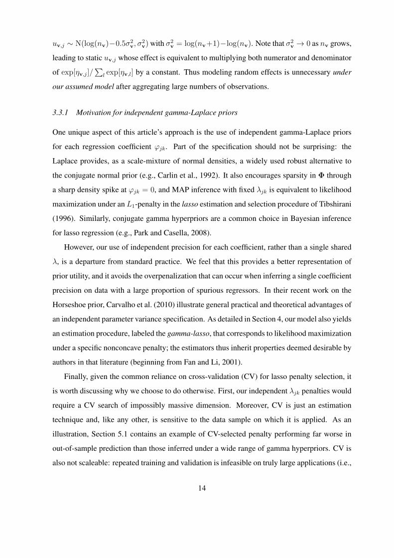
3.3.1 Motivation for independent gamma-Laplace priors

One unique aspect of this article’s approach is the use of independent gamma-Laplace priors

for each regression coefficient ϕjk. Part of the specification should not be surprising: the

Laplace provides, as a scale-mixture of normal densities, a widely used robust alternative to

the conjugate normal prior (e.g., Carlin et al., 1992). It also encourages sparsity in Φ through

a sharp density spike at ϕjk = 0, and MAP inference with fixed λjk is equivalent to likelihood

maximization under an L1-penalty in the lasso estimation and selection procedure of Tibshirani

(1996). Similarly, conjugate gamma hyperpriors are a common choice in Bayesian inference

for lasso regression (e.g., Park and Casella, 2008).

However, our use of independent precision for each coefficient, rather than a single shared

λ, is a departure from standard practice. We feel that this provides a better representation of

prior utility, and it avoids the overpenalization that can occur when inferring a single coefficient

precision on data with a large proportion of spurious regressors. In their recent work on the

Horseshoe prior, Carvalho et al. (2010) illustrate general practical and theoretical advantages of

an independent parameter variance specification. As detailed in Section 4, our model also yields

an estimation procedure, labeled the gamma-lasso, that corresponds to likelihood maximization

under a specific nonconcave penalty; the estimators thus inherit properties deemed desirable by

authors in that literature (beginning from Fan and Li, 2001).

Finally, given the common reliance on cross-validation (CV) for lasso penalty selection, it

is worth discussing why we choose to do otherwise. First, our independent λjk penalties would

require a CV search of impossibly massive dimension. Moreover, CV is just an estimation

technique and, like any other, is sensitive to the data sample on which it is applied. As an

illustration, Section 5.1 contains an example of CV-selected penalty performing far worse in

out-of-sample prediction than those inferred under a wide range of gamma hyperpriors. CV is

also not scaleable: repeated training and validation is infeasible on truly large applications (i.e.,

14

when estimating the model once is expensive). That said, one may wish to use CV to choose

s or r in the hyperprior; since results are less sensitive to these parameters than they are to a

fixed penalty, a small grid of search locations should suffice.

4 Estimation

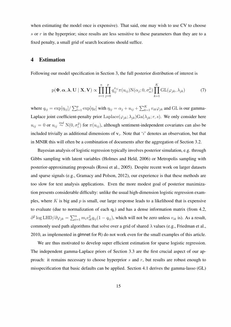
Following our model specification in Section 3, the full posterior distribution of interest is

p(Φ,α,λ,U | X,V) ∝n∏i=1

p∏j=0

qxijij π(uij)N(αj; 0, σ2

α)K∏k=1

GL(ϕjk, λjk) (7)

where qij = exp[ηij]/∑p

l=1 exp[ηil] with ηij = αj + uij +∑K

k=1 vikϕjk and GL is our gamma-

Laplace joint coefficient-penalty prior Laplace(ϕjk;λjk)Ga(λjk; r, s). We only consider here

uij = 0 or uijind∼ N(0, σ2

i ) for π(uij), although sentiment-independent covariates can also be

included trivially as additional dimensions of vi. Note that ‘i’ denotes an observation, but that

in MNIR this will often be a combination of documents after the aggregation of Section 3.2.

Bayesian analysis of logistic regression typically involves posterior simulation, e.g. through

Gibbs sampling with latent variables (Holmes and Held, 2006) or Metropolis sampling with

posterior-approximating proposals (Rossi et al., 2005). Despite recent work on larger datasets

and sparse signals (e.g., Gramacy and Polson, 2012), our experience is that these methods are

too slow for text analysis applications. Even the more modest goal of posterior maximiza-

tion presents considerable difficulty: unlike the usual high-dimension logistic regression exam-

ples, where K is big and p is small, our large response leads to a likelihood that is expensive

to evaluate (due to normalization of each qi) and has a dense information matrix (from 4.2,

∂2 log LHD/∂ϕjk =∑n

i=1miv2ikqij(1− qij), which will not be zero unless vik is). As a result,

commonly used path algorithms that solve over a grid of shared λ values (e.g., Friedman et al.,

2010, as implemented in glmnet for R) do not work even for the small examples of this article.

We are thus motivated to develop super efficient estimation for sparse logistic regression.

The independent gamma-Laplace priors of Section 3.3 are the first crucial aspect of our ap-

proach: it remains necessary to choose hyperprior s and r, but results are robust enough to

misspecification that basic defaults can be applied. Section 4.1 derives the gamma-lasso (GL)

15

non-concave penalty that results from MAP estimation under this prior. Second, Section 4.2

describes a coordinate descent algorithm for fast negative log posterior minimization wherein

the GL penalties are incorporated at no extra cost over standard lasso regression. Lastly, 4.3

considers conditions for posterior log concavity and convergence.

4.1 Gamma-lasso penalized regression

Our estimation framework relies upon recognition that optimal λjk can always be written as a

function of ϕjk, and thus does not need to be explicitly solved for in the joint objective.

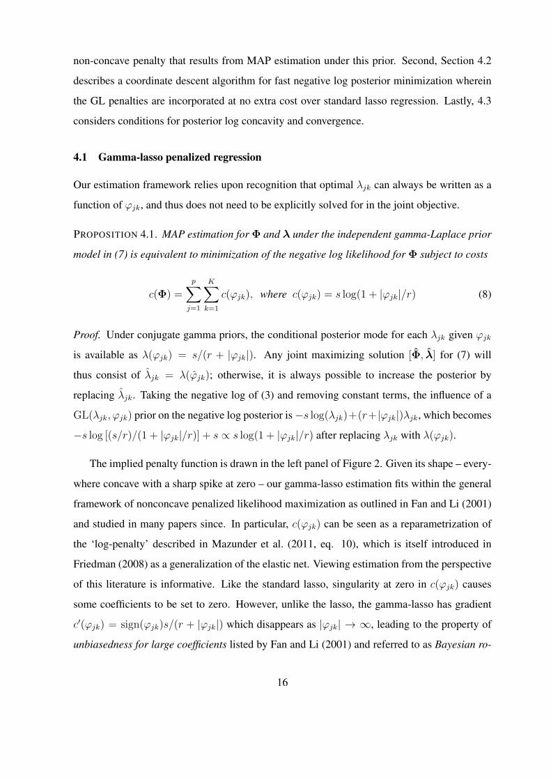
PROPOSITION 4.1. MAP estimation for Φ and λ under the independent gamma-Laplace prior

model in (7) is equivalent to minimization of the negative log likelihood for Φ subject to costs

c(Φ) =

p∑j=1

K∑k=1

c(ϕjk), where c(ϕjk) = s log(1 + |ϕjk|/r) (8)

Proof. Under conjugate gamma priors, the conditional posterior mode for each λjk given ϕjk

is available as λ(ϕjk) = s/(r + |ϕjk|). Any joint maximizing solution [Φ, λ] for (7) will

thus consist of λjk = λ(ϕjk); otherwise, it is always possible to increase the posterior by

replacing λjk. Taking the negative log of (3) and removing constant terms, the influence of a

GL(λjk, ϕjk) prior on the negative log posterior is−s log(λjk)+(r+ |ϕjk|)λjk, which becomes

−s log [(s/r)/(1 + |ϕjk|/r)] + s ∝ s log(1 + |ϕjk|/r) after replacing λjk with λ(ϕjk).

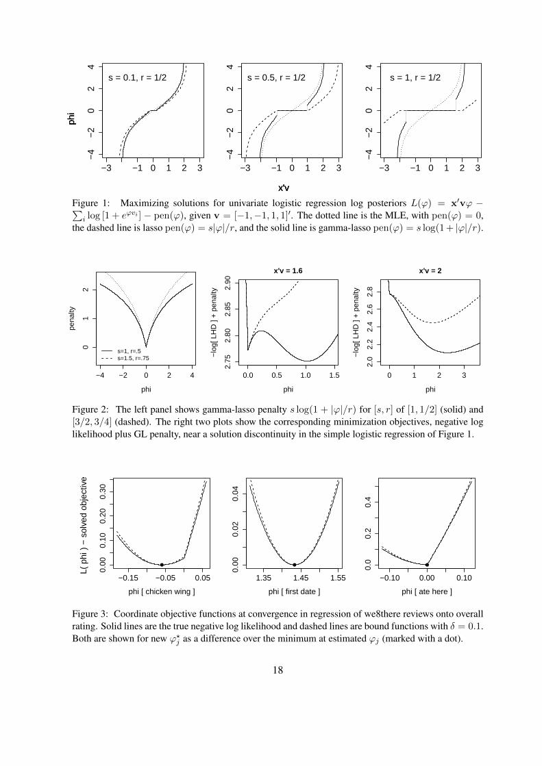
The implied penalty function is drawn in the left panel of Figure 2. Given its shape – every-

where concave with a sharp spike at zero – our gamma-lasso estimation fits within the general

framework of nonconcave penalized likelihood maximization as outlined in Fan and Li (2001)

and studied in many papers since. In particular, c(ϕjk) can be seen as a reparametrization of

the ‘log-penalty’ described in Mazunder et al. (2011, eq. 10), which is itself introduced in

Friedman (2008) as a generalization of the elastic net. Viewing estimation from the perspective

of this literature is informative. Like the standard lasso, singularity at zero in c(ϕjk) causes

some coefficients to be set to zero. However, unlike the lasso, the gamma-lasso has gradient

c′(ϕjk) = sign(ϕjk)s/(r + |ϕjk|) which disappears as |ϕjk| → ∞, leading to the property of

unbiasedness for large coefficients listed by Fan and Li (2001) and referred to as Bayesian ro-

16

bustness by Carvalho et al. (2010). Other results from this literature apply directly; for example,

in most problems it should be possible to choose s and r to satisfy requirements for the strong

oracle property of Fan and Peng (2004) conditional on their various likelihood conditions.

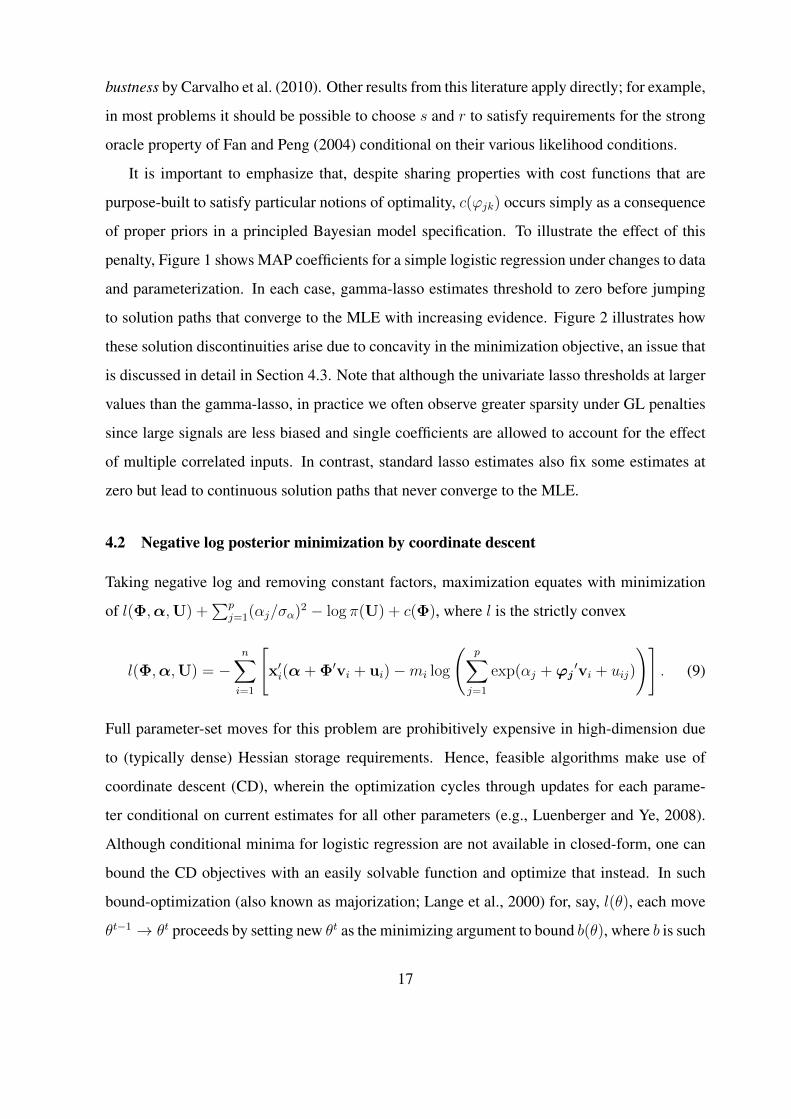
It is important to emphasize that, despite sharing properties with cost functions that are

purpose-built to satisfy particular notions of optimality, c(ϕjk) occurs simply as a consequence

of proper priors in a principled Bayesian model specification. To illustrate the effect of this

penalty, Figure 1 shows MAP coefficients for a simple logistic regression under changes to data

and parameterization. In each case, gamma-lasso estimates threshold to zero before jumping

to solution paths that converge to the MLE with increasing evidence. Figure 2 illustrates how

these solution discontinuities arise due to concavity in the minimization objective, an issue that

is discussed in detail in Section 4.3. Note that although the univariate lasso thresholds at larger

values than the gamma-lasso, in practice we often observe greater sparsity under GL penalties

since large signals are less biased and single coefficients are allowed to account for the effect

of multiple correlated inputs. In contrast, standard lasso estimates also fix some estimates at

zero but lead to continuous solution paths that never converge to the MLE.

4.2 Negative log posterior minimization by coordinate descent

Taking negative log and removing constant factors, maximization equates with minimization

of l(Φ,α,U) +∑p

j=1(αj/σα)2 − log π(U) + c(Φ), where l is the strictly convex

l(Φ,α,U) = −n∑i=1

[x′i(α+ Φ′vi + ui)−mi log

(p∑j=1

exp(αj +ϕj′vi + uij)

)]. (9)

Full parameter-set moves for this problem are prohibitively expensive in high-dimension due

to (typically dense) Hessian storage requirements. Hence, feasible algorithms make use of

coordinate descent (CD), wherein the optimization cycles through updates for each parame-

ter conditional on current estimates for all other parameters (e.g., Luenberger and Ye, 2008).

Although conditional minima for logistic regression are not available in closed-form, one can

bound the CD objectives with an easily solvable function and optimize that instead. In such

bound-optimization (also known as majorization; Lange et al., 2000) for, say, l(θ), each move

θt−1 → θt proceeds by setting new θt as the minimizing argument to bound b(θ), where b is such

17

−3 −1 0 1 2 3

−4

−2

02

4s = 0.1, r = 1/2

x'v

phi

−3 −1 0 1 2 3

−4

−2

02

4

s = 0.5, r = 1/2

x'v

phi

−3 −1 0 1 2 3

−4

−2

02

4

s = 1, r = 1/2

x'v

phi

Figure 1: Maximizing solutions for univariate logistic regression log posteriors L(ϕ) = x′vϕ −∑i log [1 + eϕvi ] − pen(ϕ), given v = [−1,−1, 1, 1]′. The dotted line is the MLE, with pen(ϕ) = 0,

the dashed line is lasso pen(ϕ) = s|ϕ|/r, and the solid line is gamma-lasso pen(ϕ) = s log(1+ |ϕ|/r).

−4 −2 0 2 4

phi

pena

lty

01

2

s=1, r=.5s=1.5, r=.75

0.0 0.5 1.0 1.5

2.75

2.80

2.85

2.90

x'v = 1.6

phi

−lo

g[ L

HD

] +

pen

alty

0 1 2 32.

02.

22.

42.

62.

8

x'v = 2

phi

−lo

g[ L

HD

] +

pen

alty

Figure 2: The left panel shows gamma-lasso penalty s log(1 + |ϕ|/r) for [s, r] of [1, 1/2] (solid) and[3/2, 3/4] (dashed). The right two plots show the corresponding minimization objectives, negative loglikelihood plus GL penalty, near a solution discontinuity in the simple logistic regression of Figure 1.

−0.15 −0.05 0.05

0.00

0.10

0.20

0.30

phi [ chicken wing ]

●

1.35 1.45 1.55

0.00

0.02

0.04

phi [ first date ]

●

−0.10 0.00 0.10

0.0

0.2

0.4

phi [ ate here ]

●

L

( ph

i ) −

sol

ved

obje

ctiv

e

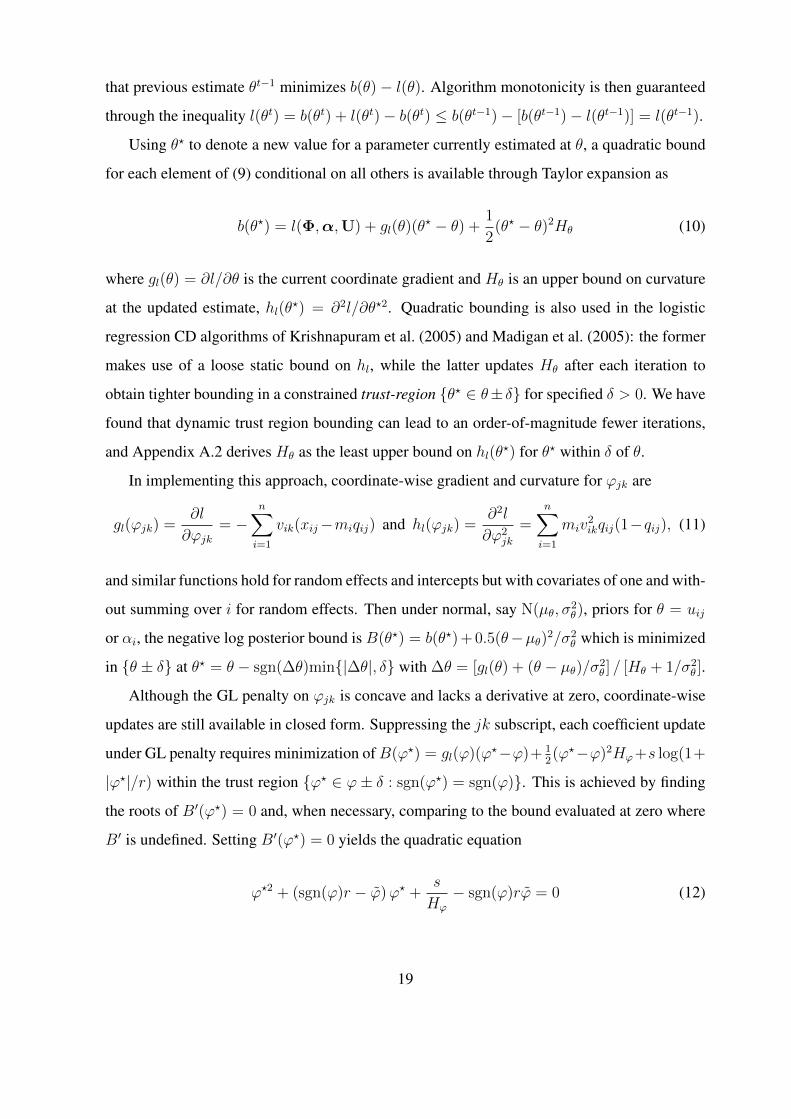
Figure 3: Coordinate objective functions at convergence in regression of we8there reviews onto overallrating. Solid lines are the true negative log likelihood and dashed lines are bound functions with δ = 0.1.Both are shown for new ϕ?j as a difference over the minimum at estimated ϕj (marked with a dot).

18

that previous estimate θt−1 minimizes b(θ)− l(θ). Algorithm monotonicity is then guaranteed

through the inequality l(θt) = b(θt) + l(θt)− b(θt) ≤ b(θt−1)− [b(θt−1)− l(θt−1)] = l(θt−1).

Using θ? to denote a new value for a parameter currently estimated at θ, a quadratic bound

for each element of (9) conditional on all others is available through Taylor expansion as

b(θ?) = l(Φ,α,U) + gl(θ)(θ? − θ) +

1

2(θ? − θ)2Hθ (10)

where gl(θ) = ∂l/∂θ is the current coordinate gradient and Hθ is an upper bound on curvature

at the updated estimate, hl(θ?) = ∂2l/∂θ?2. Quadratic bounding is also used in the logistic

regression CD algorithms of Krishnapuram et al. (2005) and Madigan et al. (2005): the former

makes use of a loose static bound on hl, while the latter updates Hθ after each iteration to

obtain tighter bounding in a constrained trust-region {θ? ∈ θ± δ} for specified δ > 0. We have

found that dynamic trust region bounding can lead to an order-of-magnitude fewer iterations,

and Appendix A.2 derives Hθ as the least upper bound on hl(θ?) for θ? within δ of θ.

In implementing this approach, coordinate-wise gradient and curvature for ϕjk are

gl(ϕjk) =∂l

∂ϕjk= −

n∑i=1

vik(xij−miqij) and hl(ϕjk) =∂2l

∂ϕ2jk

=n∑i=1

miv2ikqij(1−qij), (11)

and similar functions hold for random effects and intercepts but with covariates of one and with-

out summing over i for random effects. Then under normal, say N(µθ, σ2θ), priors for θ = uij

or αi, the negative log posterior bound is B(θ?) = b(θ?) + 0.5(θ−µθ)2/σ2θ which is minimized

in {θ ± δ} at θ? = θ − sgn(∆θ)min{|∆θ|, δ} with ∆θ = [gl(θ) + (θ − µθ)/σ2θ ] / [Hθ + 1/σ2

θ ].

Although the GL penalty on ϕjk is concave and lacks a derivative at zero, coordinate-wise

updates are still available in closed form. Suppressing the jk subscript, each coefficient update

under GL penalty requires minimization ofB(ϕ?) = gl(ϕ)(ϕ?−ϕ)+ 12(ϕ?−ϕ)2Hϕ+s log(1+

|ϕ?|/r) within the trust region {ϕ? ∈ ϕ± δ : sgn(ϕ?) = sgn(ϕ)}. This is achieved by finding

the roots of B′(ϕ?) = 0 and, when necessary, comparing to the bound evaluated at zero where

B′ is undefined. Setting B′(ϕ?) = 0 yields the quadratic equation

ϕ?2 + (sgn(ϕ)r − ϕ)ϕ? +s

Hϕ

− sgn(ϕ)rϕ = 0 (12)

19

with characteristic (sgn(ϕ)r + ϕ)2 − 4s/Hϕ, where ϕ = ϕ− gl(ϕ)/Hϕ would be the updated

coordinate for an MLE estimator. From standard techniques, for {ϕ? : sgn(ϕ) = sgn(ϕ?)}

this function will have at most one real minimizing root – that is, with Hϕ > s/ (r + |ϕ?|)2.

Hence, each coordinate update is to find this root (if it exists) and compare B(ϕ?) to B(0). The

minimizing value (0 or possible root ϕ?) dictates our parameter move ∆ϕ, and this move is

truncated at sgn(∆ϕ)δ if it exceeds the trust region. Finally, when ϕ = 0, repeat this procedure

for both sgn(ϕ) = ±1; at most one direction will lead to a nonzero solution.

As it is inexpensive to characterize roots for B′(ϕ?), the gamma-lasso does not lead to any

noticeable increase in computation time over standard lasso algorithms (e.g., Madigan et al.,

2005). Crucially, tests for decreased objective can performed on the bound function, instead

of the full negative log posterior. Figure 3 shows objective and bound functions around the

converged solution for three phrase loadings from regression of we8there reviews onto overall

rating. With δ = 0.1, B provides tight bounding throughout this neighborhood. Behavior

around the origin is most interesting: the solution for chicken wing, a low-loading negative

term, is at B′(ϕ?) = 0 just left of the singularity at zero, while ate here falls in the sharp point

at zero. The neighborhood around first date, a high-loading term, is everywhere smooth.

4.3 Posterior log concavity and algorithm convergence

Since the gamma-lasso penalty is everywhere concave, our minimization objective is not guar-

anteed to be convex. This is illustrated by the right two plots of Figure 2, where a very low-

information likelihood (four observations) can be combined with a relatively diffuse prior on λ

(s = 1, r = 1/2) to yield concavity near zero. The effect of this is benign when the gradient

is the same direction on either side of the origin (as in the right panel of 2), but in other cases

it will lead to local minima at zero away from the true global solution (as in the center panel).

Such non-convexity is the cause of the discontinuities in the solution paths of Figure 1.

From the second derivative of l(ϕjk) + c(ϕjk), the conditional objective for ϕjk will be

concave only if hl(ϕjk = 0) < s/r2 – that is, if prior variance on λjk is greater than the

negative log likelihood curvature at ϕjk = 0. In our experience, this problem is rare: the

likelihood typically overwhelms penalty concavity and real examples behave like those shown

in Figure 3. Moreover, although it is possible to show stationary limit points for CD on such

20

nonconvex functions (e.g. Mazunder et al., 2011), we advocate avoiding the issue through prior

specification. In particular, hyperprior shape and rate can be raised to decrease var(λjk) while

keeping E[λjk] unchanged. Although this may require more prior information than desired, it

is the amount necessary to have both fast MAP estimation and estimator stability. If you want

to use more diffuse priors, you should pay the computational price of marginalization and mean

inference (as in, e.g., Gramacy and Polson, 2012).

5 Examples

We now apply our framework to the datasets of Section 1.1. The implemented software is

available as the textir package for R, with these examples included as demos. Section 5.1

examines out-of-sample predictive performance, and is followed by individual data analyses.

5.1 A comparison of text regression methods

Our prediction performance study considers three text analyses: both constituent percentage

vote-share for G.W. Bush (bushvote) and Republican party membership (gop) regressed onto

speech for a member of the 109th US congress, and a user’s overall rating (overall) regressed

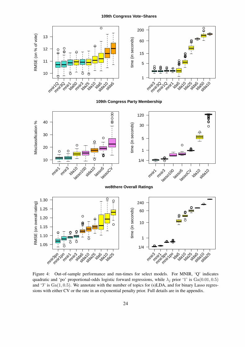
onto the content of their we8there restaurant review. In each case, we report root mean square

error or misclassification rate over 100 training and validation iterations. Full results and study

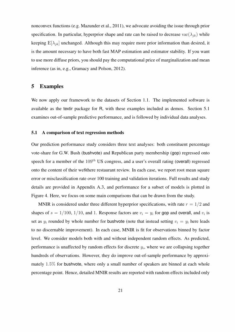
details are provided in Appendix A.3, and performance for a subset of models is plotted in

Figure 4. Here, we focus on some main comparisons that can be drawn from the study.

MNIR is considered under three different hyperprior specifications, with rate r = 1/2 and

shapes of s = 1/100, 1/10, and 1. Response factors are vi = yi for gop and overall, and vi is

set as yi rounded by whole number for bushvote (note that instead setting vi = yi here leads

to no discernable improvement). In each case, MNIR is fit for observations binned by factor

level. We consider models both with and without independent random effects. As predicted,

performance is unaffected by random effects for discrete yi, where we are collapsing together

hundreds of observations. However, they do improve out-of-sample performance by approxi-

mately 1.5% for bushvote, where only a small number of speakers are binned at each whole

percentage point. Hence, detailed MNIR results are reported with random effects included only

21

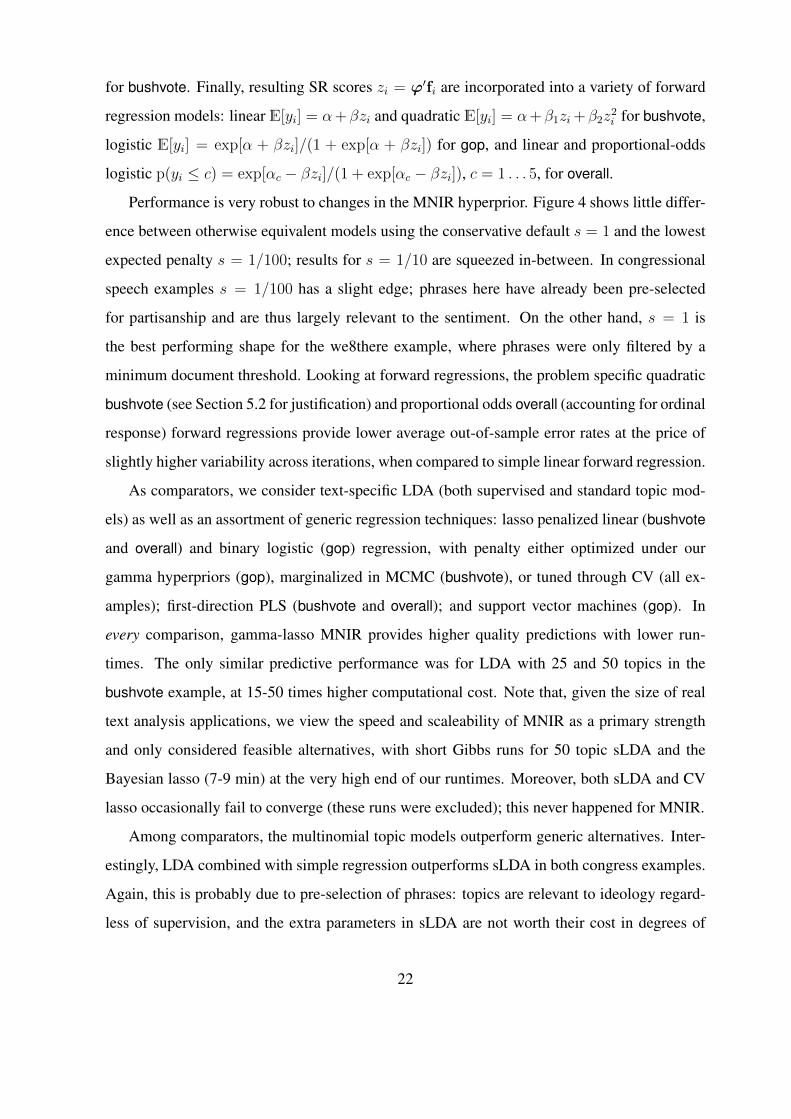
for bushvote. Finally, resulting SR scores zi = ϕ′fi are incorporated into a variety of forward

regression models: linear E[yi] = α+βzi and quadratic E[yi] = α+β1zi +β2z2i for bushvote,

logistic E[yi] = exp[α + βzi]/(1 + exp[α + βzi]) for gop, and linear and proportional-odds

logistic p(yi ≤ c) = exp[αc − βzi]/(1 + exp[αc − βzi]), c = 1 . . . 5, for overall.

Performance is very robust to changes in the MNIR hyperprior. Figure 4 shows little differ-

ence between otherwise equivalent models using the conservative default s = 1 and the lowest

expected penalty s = 1/100; results for s = 1/10 are squeezed in-between. In congressional

speech examples s = 1/100 has a slight edge; phrases here have already been pre-selected

for partisanship and are thus largely relevant to the sentiment. On the other hand, s = 1 is

the best performing shape for the we8there example, where phrases were only filtered by a

minimum document threshold. Looking at forward regressions, the problem specific quadratic

bushvote (see Section 5.2 for justification) and proportional odds overall (accounting for ordinal

response) forward regressions provide lower average out-of-sample error rates at the price of

slightly higher variability across iterations, when compared to simple linear forward regression.

As comparators, we consider text-specific LDA (both supervised and standard topic mod-

els) as well as an assortment of generic regression techniques: lasso penalized linear (bushvote

and overall) and binary logistic (gop) regression, with penalty either optimized under our

gamma hyperpriors (gop), marginalized in MCMC (bushvote), or tuned through CV (all ex-

amples); first-direction PLS (bushvote and overall); and support vector machines (gop). In

every comparison, gamma-lasso MNIR provides higher quality predictions with lower run-

times. The only similar predictive performance was for LDA with 25 and 50 topics in the

bushvote example, at 15-50 times higher computational cost. Note that, given the size of real

text analysis applications, we view the speed and scaleability of MNIR as a primary strength

and only considered feasible alternatives, with short Gibbs runs for 50 topic sLDA and the

Bayesian lasso (7-9 min) at the very high end of our runtimes. Moreover, both sLDA and CV

lasso occasionally fail to converge (these runs were excluded); this never happened for MNIR.

Among comparators, the multinomial topic models outperform generic alternatives. Inter-

estingly, LDA combined with simple regression outperforms sLDA in both congress examples.

Again, this is probably due to pre-selection of phrases: topics are relevant to ideology regard-

less of supervision, and the extra parameters in sLDA are not worth their cost in degrees of

22

freedom. Moreover, the simpler LDA models can be fit with the MAP estimation of Taddy

(2012b), whereas sLDA is applied here through a slow-to-converge Gibbs sampler (we note

that the original sLDA paper uses a variational EM algorithm). However, in the we8there data,

the extra machinery of sLDA offers a clear improvement over unsupervised LDA, as should

be the case in many text applications. Finally, in an important side comparison, binary logistic

regressions were fit for gop regressed onto phrase frequencies using both CV and independent

gamma hyperpriors for the lasso penalty. The scaleable, low-cost, gamma-lasso yields large

performance improvements over a CV optimized model, regardless of hyperprior specification.

5.2 Application: partisanship and ideology in political speeches

For the data of Section 1.1.1, we have two sentiment metrics of interest: an indicator for party

membership, and each speaker’s constituent vote-share for Bush in 2004. Since the two inde-

pendents caucused with Democrats, the former metric can be summarized in gop as a two-party

partisanship. Following the political economy notion that there should be little discrepancy be-

tween voter and representative beliefs, bushvote provides a measure of ideology as expressed

in support for G.W. Bush (and lack of support for John Kerry) in the context of that election.

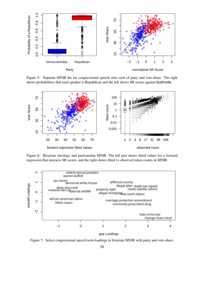
Figure 5 shows MNIR fit in separate models for each of gop and bushvote, as studied

in Section 5.1. For partisanship, fit with s = 1/100 and r = 1/2, a simple univariate lo-

gistic forward regression yields clear discrimination between parties; 8.5% (45 speakers) are

misclassified under a maximum probability rule. In the bushvote MNIR, fit under the same

hyperprior but with inclusion of random effects, the resulting SR scores zi = ϕ′fi increase

quickly with vote-share at low (mostly Democrat) values and more slowly for high (mostly Re-

publican) values. This motivates our quadratic forward regression for bushvote onto SR score,

the predictive mean of which is plotted in Figure 5 (with R2 of 0.5). However, looking at the

SR scores colored by party (red for Republicans, blue Democrats, green independents) shows

that this curvature could instead be explained through different forward regression slopes by

level of gop, implying that the relationship between language and ideology is party-dependent.

Given the above, a more useful model might consider text reduction that allows interaction

between party and ideology. For example, we can build orthogonal bivariate sentiment factors

as gop and bushvote minus the gop-level means, say votediff (again, rounded to the nearest

23

●

●

●

●

●●

●

●

● ●

●

●

10

11

12

13R

MS

E (

on %

of v

ote)

mnir

1Q

mnir

3Qm

nir1lda

50m

nir3lda

25lda

10 lda5

slda1

0sld

a5

●●●

●●●●

●● ●

●●●●●●

●●●

●

●●●

●●●

●●

time

(in s

econ

ds)

mnir

3

mnir

3Q

mnir

1Qm

nir1

lda5lda

10lda

25sld

a5lda

50

slda1

01

5

15

60

200

109th Congress Vote−Shares

● ●

●

●●

●

●●●

●

●

●

●

●

●

10

20

30

40

Mis

clas

sific

atio

n %

mnir

1m

nir3

lda10

lasso

100

slda1

0

lasso

5

lasso

CV

●

●

●

●

●●●●●●

●

●

●●

●

●

●

●●●

●

●●

time

(in s

econ

ds)

mnir

1m

nir3

lasso

100

lasso

5

lasso

CVlda

10

slda1

0

1/4

1

5

30

120

109th Congress Party Membership

●

●

●●

●

●●

●

●●●●

●

●

●

●

●

●

1.05

1.10

1.15

1.20

1.25

1.30

RM

SE

(on

ove

rall

ratin

g)

mnir

3po

mnir

1po

mnir

1m

nir3sld

a5

slda1

0

slda2

5lda

5lda

10lda

25

●●●●●

●●●● ●●●●●●

●●

●●●

●

●●

●

time

(in s

econ

ds)

mnir

3m

nir1

mnir

3po

mnir

1po

lda5lda

10lda

25sld

a5

slda1

0

slda2

5

1/4

1

10

60

240

we8there Overall Ratings

Figure 4: Out-of-sample performance and run-times for select models. For MNIR, ‘Q’ indicatesquadratic and ‘po’ proportional-odds logistic forward regressions, while λj prior ‘1’ is Ga(0.01, 0.5)and ‘3’ is Ga(1, 0.5). We annotate with the number of topics for (s)LDA, and for binary Lasso regres-sions with either CV or the rate in an exponential penalty prior. Full details are in the appendix.

24

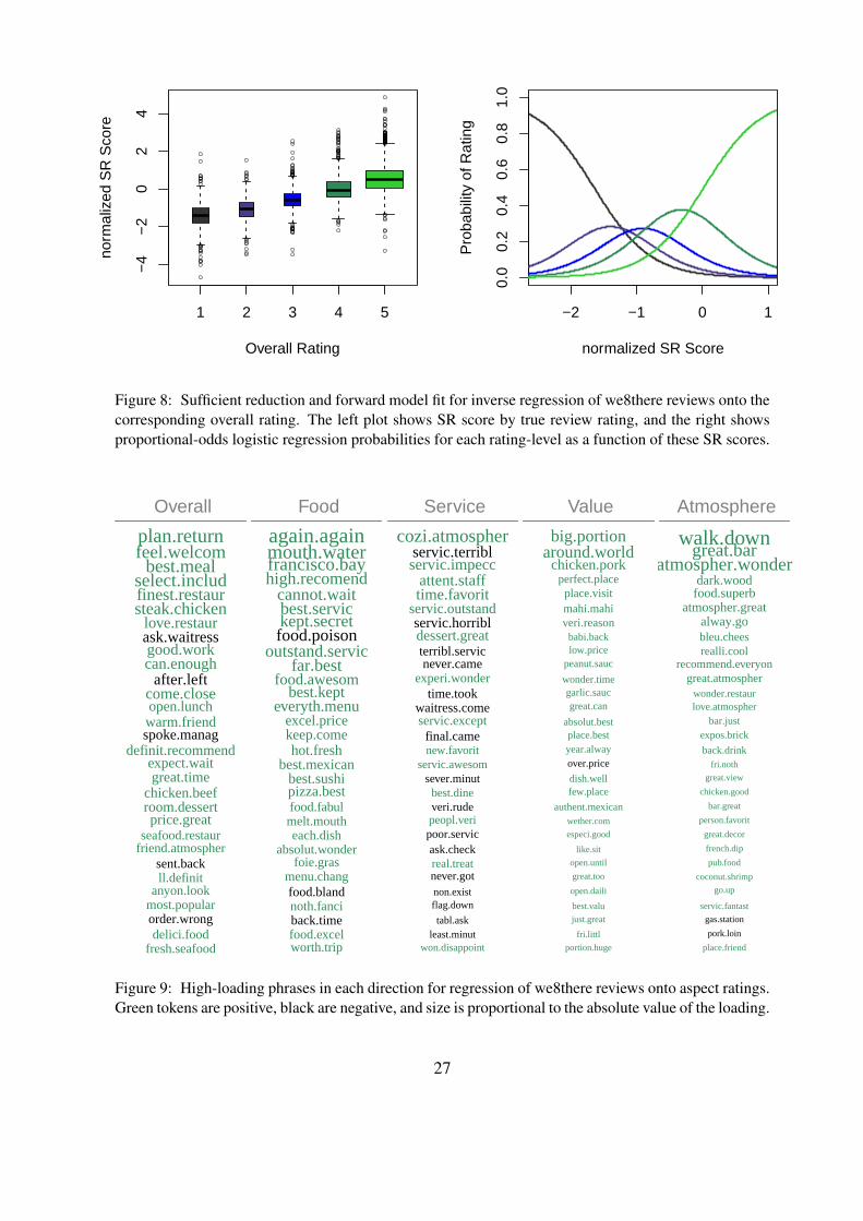
whole percentage). Figure 6 shows fitted values for such a model, including random effects

and with hyperprior shape increased to s = 1/10 to reflect a preference for smaller conditional

coefficients. In detail, with zgop and zvotediff the two dimensions of SR scores from MNIR

x ∼ MN(q(vgop, vvotediff),m), normalized for ease of interpretation, the fitted forward model is

E[bushvote] = 51.9 + 6.2zgop + 5.2zvotediff − 1.9zgopzvotediff . (13)

Thus a standard deviation increase in either SR direction implies a 5-6% increase in expected

vote-share, and each effect is dampened when the normalized SR scores have the same sign.

The right panel of Figure 6 shows fitted expected counts qjm against true nonzero counts

in our bivariate MNIR model fit; with random effects to account for model misspecification,

there appears to be no pattern of overdispersion. The only clear outlier in forward regression

is Chaka Fattah (D-PA) with a standardized residual of -5.2; he uttered a token in our sample

only twice: once each for rate.return and billion.dollar. Finally, Figure 7 plots response factor

loadings for a select group of tokens. Among other lessons, we see that racial identity rhetoric

(african.american.latino, black.caucu) points towards the left wing of the Democratic party,

while discussion of hate crimes is indicative of a moderate Republican. A few large loadings are

driven by single observations: for example, violent.sexual.predator contributes more than 0.1%

of speech for only Byron Dorgan, a Democratic Senator in Bush-supporting North Dakota.

However, this is not the rule and most term loadings affect many speakers.

5.3 Application: on-line restaurant reviews

For the data of Section 1.1.2, our sentiment consists of five correlated restaurant ratings (each

on a five point scale) that accompany every review. The left panel of Figure 8 shows MNIR

for review content regressed onto the single overall response factor, as studied in Section 5.1.

The true overall rating has high correlation (0.7) with our SR scores, despite considerable over-

lap between scores across rating levels. The right plot of Figure 8 shows probabilities for each

increasing overall rating category, as estimated in the proportional-odds logistic forward regres-

sion, p(overall ≤ c) = exp[αc−βzoverall]/(1 + exp[αc−βzoverall]). Again, zoverall is normalized

here to have mean zero and standard deviation of one in our sample. This model has β = 2.3,

25

●

●●

●

●

●

●

●

●

●

●

●

●

●

●●

●

●●

●

●

●

●

●

●

●●●

●

●

●●

●

●

●

●

●

●

●

●●

●

●

●

●

●

●

●

●

●

●●

●

●

●

●

●

●

●

●

●

●

●

●

●

●

●●

●

●

●

●

●

●●

0.0

0.2

0.4

0.6

0.8

1.0

Democrat/Indep. Republican

Party

Pro

babi

lity

of a

Rep

ublic

an

●●

−2 −1 0 1 2 3

1030

5070

normalized SR Score

Vot

e S

hare

Figure 5: Separate MNIR fits for congressional speech onto each of party and vote-share. The rightshows probabilities that each speaker is Republican and the left shows SR scores against bushvote.

●●

20 30 40 50 60 70

1030

5070

forward regression fitted values

Vot

e S

hare ●●●●●

●●●●●

●●●●●●●●●

●●

●

●●●●●

●●●

●●●●

●

●●

●●

●●●●●

●●

●●●●●●●●

●●●

●

●●●●

●●●●

●

●●●●●●●●●

●

●●

●

●

●

●

●

●●●●●

●

●

●●●●●

●●●●●

●●●

●

●●●●●●

●

●●

●●●●

●

●

●

●

●●●●●●●●●●●●●●●

●

●●●●●●●

●●●

●●

●

●

●●●●●●●●●

●

●●●●

●

●

●

●●●●

●●●●●

●

●●●●

●●●●

●

●

●●●●●●●

●

●●●

●

●●

●●

●

●●●●

●

●

●

●●●

●●●●●

●

●

●

●●●●●

●

●●●●●

●●●●

●●

●

●●●●

●

●●●●●

●●

●●

●

●

●●●●

●

●●●

●

●

●

●●●

●

●●

●

●

●

●

●

●●●●●

●

●

●

●

●●●●●●●●

●

●

●●

●

●

●

●●●●●

●

●

●●

●

●●

●

●●●

●

●

●

●●●●●

●●

●●

●

●

●

●

●●●●●

●

●

●●

●●

●●●●●●●

●

●

●

●

●

●

●

●

●

●●●

●●●

●

●●●

●

●

●●

●

●

●

●

●

●●●●●●

●

●

●

●

●

●

●

●●

●

●

●●●●●●

●●

●

●●●●

●●●●●●●

●

●

●

●

●

●

●

●●●

●●●

●●

●

●●●

●●●●

●

●

●

●●

●

●●●

●●●●●

●

●

●

●

●●

●

●

●

●●●●●

●

●

●●

●

●●●

●

●●

●●

●●

●●

●●

●●

●

●●

●●

●●

●

●●●

●●

●●

●●

●

●

●

●

●●

●●

●●

●

●

●●●

●●

●●

●●

●●●

●●

●

●

●●

●

●

●●

●

●

●

●

●●●●

●●●

●●

●

●

●

●●●●

●

●

●●

●●

●

●●

●

●

●

●

●

●

●

●●

●

●●

●

●

●

●●

●

●

●

●

●●●●●

●●●●

●

●●●●●●

●

●

●●●●●●

●●

●

●

●

●

●

●

●

●●●

●

●

●

●●●

●

●●●●●●●●●●

●●●●●

●

●●●●●

●●

●

●●●●●●

●

●●

●

●●●●

●

●●●

●●

●●

●

●●●●●●●●

●

●

●

●●●●

●

●●

●

●●●●

●

●●●●

●●●●

●

●●

●●

●●●

●●●●●

●

●●●●●●

●●

●

●●●●●

●

●

●

●

●●

●

●

●●●●

●

●●●●

●

●●

●

●

●●●

●●●

●●

●

●

●●

●●●

●●

●

●

●●●

●●●

●●●

●●●●●●●

●

●

●

●

●

●

●

●●

●●

●●●

●●●●●

●

●●●●

●

●

●

●

●

●

●

●

●●●

●

●●●●●

●

●●●

●●

●

●

●●

●

●●

●●

●●

●

●

●

●●

●

●

●

●

●●●●

●

●●●●

●

●

●●●

●●

●●●

●●

●

●●

●●

●●

●

●●

●●

●

●

●●

●●●

●

●

●

●●

●

●

●

●

●

●

●

●

●

●●

●●●

●

●

●●●●●●

●

●

● ●●●●●●●●●●●●●●●●●●●●●

●●

●

●●●●

●●

●●●

●

●

●

●

●

●

●●●●

●

●●●●●●●●

●

●●

●

●●●●●●●●●

●●

●●

●

●●●●

●

●●●●●●●

●●●●●●●●●

●

●●

●●●●●●●●●●●●●●●●

●

●●●

●

●●

●●●●●●

●●●

●●●●●●●●●●

●

●●●●●

●●

●

●

●

●

●●

●

●●

●●

●

●

●●●

●●

●

●●●●●

●

●●

●

●

●

●●

●●

●●●●●

●

●●●

●

●●

●●●

●

●●●

●

●

●

●

●

●●

●●●●●

●●●

●●●●●●●●●●●●●

●

●●

●

●●●●●●●●

●●●●●●●●●●●●●●●

●

●●●

●●●●●●●●

●●●

●

●●

●●

●

●

●●●

●●

●

●●

●

●

●

●

●●

●

●●

●●●

●

●●●●●●

●●●

●●

●

●

●

●

●

●

●

●●●

●

●

●●●●●●●●●●●●●

●

●●●●●●●●●●●

●

●●●●●●●●●

●●●

●

●●●●

●

●●●●●

●

●

●

●●●●●●

●●

●

●●

●●●

●

●●●●●●

●

●

●

●

●

●

●●

●

●●

●

●●●●●●●●●

●●●

●●

●●

●●●●●●●●●

●●

●

●●

●●●●●●●

●●●●●●●●●

●

●

●●

●

●

●●

●

●

●

●

●

●

●

●●●●

●●●●●

●

●●●

●●●●●●

●●●●

●

●

●●● ●

●●●●●●●●●●●●●●●●

●●●

●

●

●●

●

●

●

●●

●

●

●

●

●●●●

●●

●

●●●●●●●●●●

●

●●●●

●●●●●●

●

●

●●

●●●

●

●●●●●●●

●

●

●

● ●●●●●●●●●●●●●●

●

●●

●●●●●

●

●

●●●

●

●●●●

●

● ●

●

●●

●

●●

●

●●●

●●●●●

●●

●●●

●●●●●●●●

●●●●●●●

●●●●●●●

●

●●

●●●●●

●

●●

●

●

●

●●

●●●

●●●●●●●●●●

●

●●

●●●●●●●●●●

●●●●●

●●●●

●

●

●●●●●

●●●●

●●

●

●

●

●

●

●

●●● ●

●●

1 2 4 8 17 41 98 266

observed count

fitte

d co

unt

0.001

0.01

0.1

1

10

100

Figure 6: Bivariate ideology and partisanship MNIR. The left plot shows fitted values for a forwardregression that interacts SR scores, and the right shows fitted vs observed token counts in MNIR.

−1 0 1 2 3 4

−2

−1

01

2

gop Loadings

vote

diff

Load

ings

warren.buffett

tax.haven

medic.liability.reform

commonly.prescribed.drug

hate.crime.law

jefferson.countydeath.tax.repeal

violent.sexual.predator

near.earth.object

illegal.alien

marriage.protection.amendment

deep.sea.coral

african.american.latinoblack.caucu

massive.tax.cut property.rightnational.wildlife illegal.immigrant

democrat.white.house

change.heart.mind

Figure 7: Select congressional speech term loadings in bivariate MNIR with party and vote-share.

26

1 2 3 4 5

−4

−2

02

4

Overall Rating

norm

aliz

ed S

R S

core

0.0

0.2

0.4

0.6

0.8

1.0

normalized SR Score

Pro

babi

lity

of R

atin

g

−2 −1 0 1

Figure 8: Sufficient reduction and forward model fit for inverse regression of we8there reviews onto thecorresponding overall rating. The left plot shows SR score by true review rating, and the right showsproportional-odds logistic regression probabilities for each rating-level as a function of these SR scores.

plan.returnfeel.welcombest.meal

select.includfinest.restaursteak.chicken

love.restaurask.waitressgood.workcan.enough

after.leftcome.closeopen.lunchwarm.friendspoke.manag

definit.recommendexpect.waitgreat.time

chicken.beefroom.dessertprice.great

seafood.restaurfriend.atmospher

sent.backll.definit

anyon.lookmost.popularorder.wrongdelici.food

fresh.seafood

Overall

again.againmouth.waterfrancisco.bayhigh.recomend

cannot.waitbest.servickept.secretfood.poison

outstand.servicfar.best

food.awesombest.kept

everyth.menuexcel.pricekeep.comehot.fresh

best.mexicanbest.sushipizza.bestfood.fabulmelt.moutheach.dish

absolut.wonderfoie.gras

menu.changfood.blandnoth.fanciback.timefood.excelworth.trip

Food

cozi.atmospherservic.terriblservic.impecc

attent.stafftime.favorit

servic.outstandservic.horribldessert.greatterribl.servicnever.came

experi.wondertime.took

waitress.comeservic.exceptfinal.camenew.favorit

servic.awesomsever.minutbest.dineveri.rudepeopl.veripoor.servicask.checkreal.treatnever.gotnon.existflag.down

tabl.askleast.minut

won.disappoint

Service

big.portionaround.world

chicken.porkperfect.placeplace.visitmahi.mahiveri.reasonbabi.backlow.price

peanut.sauc

wonder.timegarlic.saucgreat.can

absolut.bestplace.bestyear.alwayover.price

dish.wellfew.place

authent.mexicanwether.com

especi.good

like.sit

open.until

great.too

open.daili

best.valu

just.great

fri.littl

portion.huge

Value

walk.downgreat.bar

atmospher.wonderdark.woodfood.superb

atmospher.greatalway.gobleu.cheesrealli.cool

recommend.everyongreat.atmospher

wonder.restaurlove.atmospher

bar.justexpos.brick

back.drinkfri.noth

great.view

chicken.good

bar.great

person.favorit

great.decor

french.dip

pub.food

coconut.shrimp

go.up

servic.fantast

gas.station

pork.loin

place.friend

Atmosphere

Figure 9: High-loading phrases in each direction for regression of we8there reviews onto aspect ratings.Green tokens are positive, black are negative, and size is proportional to the absolute value of the loading.

27

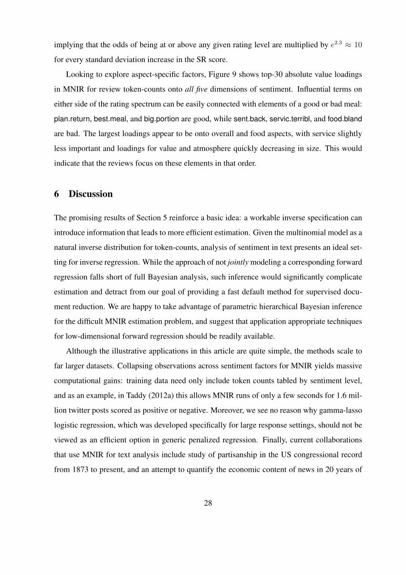
implying that the odds of being at or above any given rating level are multiplied by e2.3 ≈ 10

for every standard deviation increase in the SR score.

Looking to explore aspect-specific factors, Figure 9 shows top-30 absolute value loadings

in MNIR for review token-counts onto all five dimensions of sentiment. Influential terms on

either side of the rating spectrum can be easily connected with elements of a good or bad meal:

plan.return, best.meal, and big.portion are good, while sent.back, servic.terribl, and food.bland

are bad. The largest loadings appear to be onto overall and food aspects, with service slightly

less important and loadings for value and atmosphere quickly decreasing in size. This would

indicate that the reviews focus on these elements in that order.

6 Discussion

The promising results of Section 5 reinforce a basic idea: a workable inverse specification can

introduce information that leads to more efficient estimation. Given the multinomial model as a

natural inverse distribution for token-counts, analysis of sentiment in text presents an ideal set-

ting for inverse regression. While the approach of not jointly modeling a corresponding forward

regression falls short of full Bayesian analysis, such inference would significantly complicate

estimation and detract from our goal of providing a fast default method for supervised docu-

ment reduction. We are happy to take advantage of parametric hierarchical Bayesian inference

for the difficult MNIR estimation problem, and suggest that application appropriate techniques

for low-dimensional forward regression should be readily available.

Although the illustrative applications in this article are quite simple, the methods scale to

far larger datasets. Collapsing observations across sentiment factors for MNIR yields massive

computational gains: training data need only include token counts tabled by sentiment level,

and as an example, in Taddy (2012a) this allows MNIR runs of only a few seconds for 1.6 mil-

lion twitter posts scored as positive or negative. Moreover, we see no reason why gamma-lasso

logistic regression, which was developed specifically for large response settings, should not be

viewed as an efficient option in generic penalized regression. Finally, current collaborations

that use MNIR for text analysis include study of partisanship in the US congressional record

from 1873 to present, and an attempt to quantify the economic content of news in 20 years of

28

Wall Street Journal editions. In each case, we are considering a more rigorous treatment of the

identification of single sentiment dimensions and controlling for related endogenous variables;

this work shows MNIR’s promise as the basis for a variety of text related inference goals.

29

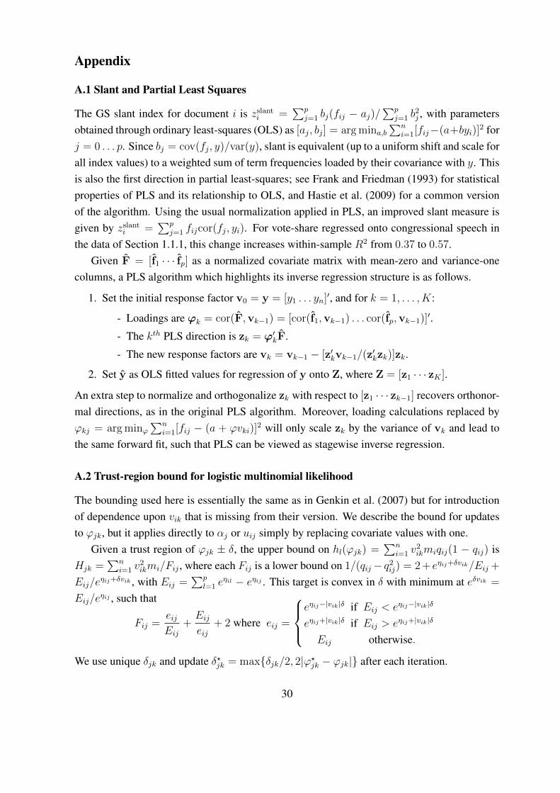
Appendix

A.1 Slant and Partial Least Squares

The GS slant index for document i is zslanti =∑p

j=1 bj(fij − aj)/∑p

j=1 b2j , with parameters

obtained through ordinary least-squares (OLS) as [aj, bj] = arg mina,b∑n

i=1[fij−(a+byi)]2 for

j = 0 . . . p. Since bj = cov(fj, y)/var(y), slant is equivalent (up to a uniform shift and scale forall index values) to a weighted sum of term frequencies loaded by their covariance with y. Thisis also the first direction in partial least-squares; see Frank and Friedman (1993) for statisticalproperties of PLS and its relationship to OLS, and Hastie et al. (2009) for a common versionof the algorithm. Using the usual normalization applied in PLS, an improved slant measure isgiven by zslanti =

∑pj=1 fijcor(fj, yi). For vote-share regressed onto congressional speech in

the data of Section 1.1.1, this change increases within-sample R2 from 0.37 to 0.57.Given F = [f1 · · · fp] as a normalized covariate matrix with mean-zero and variance-one

columns, a PLS algorithm which highlights its inverse regression structure is as follows.

1. Set the initial response factor v0 = y = [y1 . . . yn]′, and for k = 1, . . . , K:

- Loadings are ϕk = cor(F,vk−1) = [cor(f1,vk−1) . . . cor(fp,vk−1)]′.

- The kth PLS direction is zk = ϕ′kF.

- The new response factors are vk = vk−1 − [z′kvk−1/(z′kzk)]zk.

2. Set y as OLS fitted values for regression of y onto Z, where Z = [z1 · · · zK ].

An extra step to normalize and orthogonalize zk with respect to [z1 · · · zk−1] recovers orthonor-mal directions, as in the original PLS algorithm. Moreover, loading calculations replaced byϕkj = arg minϕ

∑ni=1[fij − (a + ϕvki)]

2 will only scale zk by the variance of vk and lead tothe same forward fit, such that PLS can be viewed as stagewise inverse regression.

A.2 Trust-region bound for logistic multinomial likelihood

The bounding used here is essentially the same as in Genkin et al. (2007) but for introductionof dependence upon vik that is missing from their version. We describe the bound for updatesto ϕjk, but it applies directly to αj or uij simply by replacing covariate values with one.

Given a trust region of ϕjk ± δ, the upper bound on hl(ϕjk) =∑n

i=1 v2ikmiqij(1 − qij) is

Hjk =∑n

i=1 v2ikmi/Fij , where each Fij is a lower bound on 1/(qij− q2ij) = 2 + eηij+δvik/Eij +

Eij/eηij+δvik , with Eij =

∑pl=1 e

ηil − eηij . This target is convex in δ with minimum at eδvik =

Eij/eηij , such that

Fij =eijEij

+Eijeij

+ 2 where eij =

eηij−|vik|δ if Eij < eηij−|vik|δ

eηij+|vik|δ if Eij > eηij+|vik|δ

Eij otherwise.

We use unique δjk and update δ?jk = max{δjk/2, 2|ϕ?jk − ϕjk|} after each iteration.

30

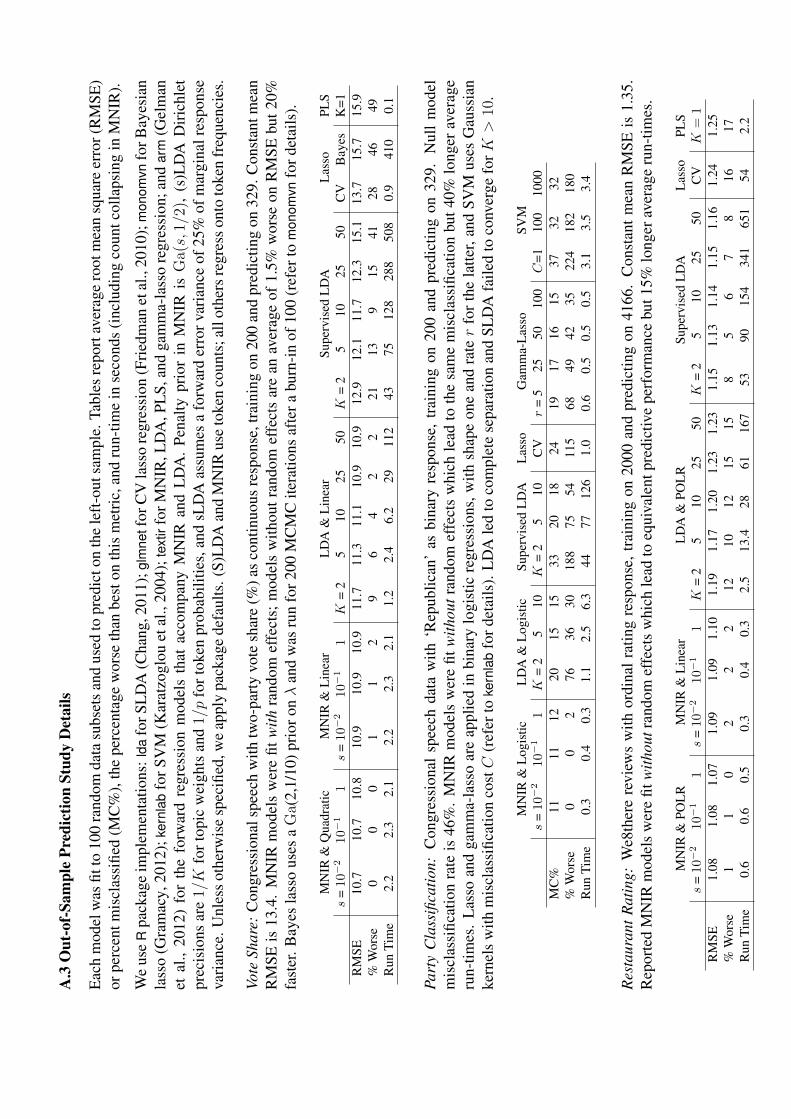
A.3

Out

-of-

Sam

ple

Pred

ictio

nSt

udy

Det

ails

Eac

hm

odel

was

fitto

100

rand

omda

tasu

bset

san

dus

edto

pred

icto

nth

ele

ft-o

utsa

mpl

e.Ta

bles

repo

rtav

erag

ero

otm

ean

squa

reer

ror(

RM

SE)

orpe

rcen

tmis

clas

sifie

d(M

C%

),th

epe

rcen

tage

wor

seth

anbe

ston

this

met

ric,

and

run-

time

inse

cond

s(i

nclu

ding

coun

tcol

laps

ing

inM

NIR

).

We

use

Rpa

ckag

eim

plem

enta

tions

:lda

forS

LD

A(C

hang

,201

1);g

lmne

tfor

CV

lass

ore

gres

sion

(Fri

edm

anet

al.,

2010

);m

onom

vnfo

rBay

esia

nla

sso

(Gra

mac

y,20

12);

kern

lab

forS

VM

(Kar

atzo

glou

etal

.,20

04);

text

irfo

rMN

IR,L

DA

,PL

S,an

dga

mm

a-la

sso

regr

essi

on;a

ndar

m(G

elm

anet

al.,

2012

)fo

rth

efo

rwar

dre

gres

sion

mod

els

that

acco

mpa

nyM

NIR

and

LD

A.

Pena

ltypr

ior

inM

NIR

isG

a(s,

1/2)

,(s

)LD

AD

iric

hlet

prec

isio

nsar

e1/K

fort

opic

wei

ghts

and

1/p

fort

oken

prob

abili

ties,

and

sLD

Aas

sum

esa

forw

ard

erro

rvar

ianc

eof

25%

ofm

argi

nalr

espo

nse

vari

ance

.Unl

ess

othe

rwis

esp

ecifi

ed,w

eap

ply

pack

age

defa

ults

.(S)

LD

Aan

dM

NIR

use

toke

nco

unts

;all

othe

rsre

gres

son

toto

ken

freq

uenc

ies.

Vote

Shar

e:C

ongr

essi

onal

spee

chw

ithtw

o-pa

rty

vote

shar

e(%

)as

cont

inuo

usre

spon

se,t

rain

ing

on20

0an

dpr

edic

ting

on32

9.C

onst

antm

ean

RM

SEis

13.4

.M

NIR

mod

els

wer

efit

with

rand

omef

fect

s;m

odel

sw

ithou

tran

dom

effe

cts

are

anav

erag

eof

1.5%

wor

seon

RM

SEbu

t20%

fast

er.B

ayes

lass

ous

esa

Ga(

2,1/

10)p

rior

onλ

and

was

run

for2

00M

CM

Cite

ratio

nsaf

tera

burn

-in

of10

0(r

efer

tom

onom

vnfo

rdet

ails

).

MN

IR&

Qua

drat

icM

NIR

&L

inea

rL

DA

&L

inea

rSu

perv

ised

LD

AL

asso

PLS

s=10

−2

10−1

1s

=10

−2

10−1

1K

=2

510

2550

K=

25

1025

50C

VB

ayes

K=1

RM

SE10

.710

.710

.810

.910

.910

.911

.711

.311

.110

.910

.912

.912

.111

.712

.315

.113

.715

.715

.9%

Wor

se0

00

11

29

64

22

2113

915

4128

4649

Run

Tim

e2.

22.

32.

12.

22.

32.

11.

22.

46.

229

112

4375

128

288

508

0.9

410

0.1

Part

yC

lass

ifica

tion:

Con

gres

sion

alsp

eech

data

with

‘Rep

ublic

an’

asbi

nary

resp

onse

,tr

aini

ngon

200

and

pred

ictin

gon

329.

Nul

lm

odel

mis

clas

sific

atio

nra

teis

46%

.M

NIR

mod

els

wer

efit

with

outr

ando

mef

fect

sw

hich

lead

toth

esa

me

mis

clas

sific

atio

nbu

t40%

long

erav

erag

eru

n-tim

es.

Las

soan

dga

mm

a-la

sso

are

appl

ied

inbi

nary

logi

stic

regr

essi

ons,

with

shap

eon

ean

dra

ter

for

the

latte

r,an

dSV

Mus

esG

auss

ian

kern

els

with

mis

clas

sific

atio

nco

stC

(ref

erto

kern

lab

ford

etai

ls).

LD

Ale

dto

com

plet

ese

para

tion

and

SLD

Afa

iled

toco

nver

gefo

rK>

10.

MN

IR&

Log

istic

LD

A&

Log

istic

Supe

rvis

edL

DA

Las

soG

amm

a-L

asso

SVM

s=10

−2

10−1

1K

=2

510

K=

25

10C

Vr

=5

2550

100

C=1

100

1000

MC

%11

1112

2015

1533

2018

2419

1716

1537

3232

%W

orse

00

276

3630

188

7554

115

6849

4235

224

182

180

Run

Tim

e0.

30.

40.

31.

12.

56.

344

7712

61.

00.

60.

50.

50.

53.

13.

53.

4

Res

taur

antR

atin

g:W

e8th

ere

revi

ews

with

ordi

nalr

atin

gre

spon

se,t

rain

ing

on20

00an

dpr

edic

ting

on41

66.

Con

stan

tmea

nR

MSE

is1.

35.

Rep

orte

dM

NIR

mod

els

wer

efit

with

outr

ando

mef

fect

sw

hich

lead

toeq

uiva

lent

pred

ictiv

epe

rfor

man

cebu

t15%

long

erav

erag

eru

n-tim

es.

MN

IR&

POL

RM

NIR

&L

inea

rL

DA

&PO

LR

Supe

rvis

edL

DA

Las

soPL

Ss

=10

−2

10−1

1s

=10

−2

10−

11

K=

25

1025

50K

=2

510

2550

CV

K=

1R

MSE

1.08

1.08

1.07

1.09

1.09

1.10

1.19

1.17

1.20

1.23

1.23

1.15

1.13

1.14

1.15

1.16

1.24

1.25

%W

orse

11

02

22

1210

1215

158

56

78

1617

Run

Tim

e0.

60.

60.

50.

30.

40.

32.

513

.428

6116

753

9015

434

165

154

2.2

References

Agresti, A. (2002). Categorical Data Analysis (2nd ed.). Wiley.

Bishop, Y., S. Fienberg, and P. Holland (1975). Discrete Multivariate Analysis. MIT Press.

Blei, D. M. and J. D. McAuliffe (2007). Supervised topic models. In Neural Information ProcessingSystems, Volume 21.

Blei, D. M., A. Y. Ng, and M. I. Jordan (2003). Latent Dirichlet allocation. Journal of Machine LearningResearch 3, 993–1022.

Bollen, J., H. Mao, and X.-J. Zeng (2011). Twitter mood predicts the stock market. Journal of Compu-tational Science 2, 1–8.

Bura, E. and D. Cook (2001). Estimating the structural dimension of regressions via parametric inverseregression. Journal of the Royal Statistical Society, Series B 63, 393–410.

Carlin, B. P., N. G. Polson, and D. S. Stoffer (1992). A Monte-Carlo approach to nonnormal andnonlinear state-space modeling. Journal of the American Statistical Association 87, 493–500.

Carvalho, C. M., N. G. Polson, and J. G. Scott (2010). The horseshoe estimator for sparse signals.Biometrika 97, 465–480.

Chang, J. (2011). lda: Collapsed Gibbs sampling methods for topic models. R package version 1.3.1.

Cook, R. D. (2007). Fisher lecture: Dimension reduction in regression. Statistical Science 22, 1–26.

Cook, R. D. and L. Li (2009). Dimension reduction in regressions with exponential family predictors.Journal of Computational and Graphical Statistics 18, 774–791.

Fan, J. and R. Li (2001). Variable selection via nonconcave penalized likelihood and its oracle properties.Journal of the American Statistical Association 96, 1348–1360.

Fan, J. and H. Peng (2004). Nonconcave penalized likelihood with a diverging number of parameters.The Annals of Statistics 32, 928–961.

Frank, I. E. and J. H. Friedman (1993). A statistical view of some chemometrics regression tools.Technometrics 35, 109–135.

Friedman, J. H. (2008). Fast sparse regression and classification. Technical Report, Dept. of Statistics,Stanford University.

Friedman, J. H., T. Hastie, and R. Tibshirani (2010). Regularization paths for generalized linear modelsvia coordinate descent.

Gail, M. H., S. Wieand, and S. Piantadosi (1984). Biased estimates of treatment effect in randomizedexperiments with nonlinear regressions and omitted covariates. Biometrika 71, 341–444.

Gelman, A., Y.-S. Su, M. Yajima, J. Hill, M. G. Pittau, J. Kerman, and T. Zheng (2012). arm: DataAnalysis Using Regression and Multilevel/Hierarchical Models. R package version 1.5-03.

Genkin, A., D. D. Lewis, and D. Madigan (2007). Large-scale Bayesian logistic regression for textcategorization. Technometrics 49, 291–304.

32

Gentzkow, M. and J. Shapiro (2010). What drives media slant? Evidence from U.S. daily newspapers.Econometrica 78, 35–72.

Gramacy, R. B. (2012). monomvn: Estimation for multivariate normal and Student-t data with monotonemissingness. R package version 1.8-10.

Gramacy, R. B. and N. G. Polson (2012). Simulation-based regularized logistic regression. BayesianAnalysis 7, 1–24.

Grimmer, J. (2010). A Bayesian hierarchical topic model for political texts: Measuring expressed agen-das in senate press releases. Political Analysis 18, 1–35.

Hastie, T., R. Tibshirani, and J. H. Friedman (2009). The Elements of Statistical Learning. Springer.

Holmes, C. C. and L. Held (2006). Bayesian auxiliary variable models for binary and multinomialregression. Bayesian Analysis 1, 145–168.

Jurafsky, D. and J. H. Martin (2009). Speech and Language Processing (2nd ed.). USA: Prentice Hall.

Karatzoglou, A., A. Smola, K. Hornik, and A. Zeileis (2004). kernlab – an S4 package for kernelmethods in R. Journal of Statistical Software 11(9), 1–20.

Krishnapuram, B., L. Carin, M. A. T. Figueiredo, and A. J. Hartemink (2005). Sparse multinomial lo-gistic regression: Fast algorithms and generalization bounds. IEEE Transactions on Pattern Analysisand Machine Intelligence 27, 957–969.

Lange, K., D. R. Hunter, and I. Yang (2000). Optimization transfer using surrogate objective functions.Journal of Computational and Graphical Statistics 9, 1–20.

Laver, M., K. Benoit, and J. Garry (2003). Extracting policy positions from political texts using wordsas data. American Political Science Review 97, 311–332.

Lehmann, E. L. and H. Sheffe (1950). Completeness, similar regions, and unbiased estimation – part 1.Sankhya: The Indian Journal of Statistics 10, 305–340.

Li, K. (1991). Sliced inverse regression for dimension reduction. Journal of the American StatisticalAssociation 86, 316–327.

Li, L., R. D. Cook, and C.-L. Tsai (2007). Partial inverse regression. Biometrika 94, 615–625.

Loughran, T. and B. McDonald (2011). When is a liability not a liability? Textual analysis, dictionaries,and 10-Ks. Journal of Finance 66, 35–65.

Luenberger, D. G. and Y. Ye (2008). Linear and Nonlinear Programming (3rd ed.). Springer.

Madigan, D., A. Genkin, D. D. Lewis, and D. Fradkin (2005). Bayesian multinomial logistic regressionfor author identification. In AIP Conference Proceedings, Volume 803.

Maua, D. D. and F. G. Cozman (2009). Representing and classifying user reviews. In ENIA ’09: VIIIEnconro Nacional de Inteligencia Artificial, Brazil.

Mazunder, R., J. H. Friedman, and T. Hastie (2011). Sparsenet: Coordinate descent with nonconvexpenalties. Journal of the American Statistical Association 106, 1125–1138.

33

Pang, B. and L. Lee (2008). Opinion mining and sentiment analysis. Foundations and Trends in Infor-mation Retrieval 1-2, 1–135.

Park, T. and G. Casella (2008). The Bayesian lasso. Journal of the American Statistical Association 103,681–686.

Poon, H. and P. Domingos (2009). Unsupervised semantic parsing. In Proceedings of the Conferenceon EMNLP.

Porter, M. F. (1980). An algorithm for suffix stripping. Program 14, 130–137.

Quinn, K., B. Monroe, M. Colaresi, M. Crespin, and D. Radev (2010). How to analyze political attentionwith minimal assumptions and costs. American Journal of Political Science 54, 209–228.

Rossi, P. E., G. M. Allenby, and R. McCulloch (2005). Bayesian Statistics and Marketing. Wiley.

Schervish, M. J. (1995). Theory of Statistics. Springer.

Srivastava, A. N. and M. Sahami (Eds.) (2009). Text Mining: Classification, Clustering, and Applica-tions. CRC Press.

Taddy, M. (2012a). Design and analysis of a text mining experiment. arXiv:1206.3776v1.

Taddy, M. (2012b). On estimation and selection for topic models. In Proceedings of the 15th Interna-tional Conference on Artificial Intelligence and Statistics (AISTATS 2012).

Talley, E. L. and D. O’Kane (2011). The measure of a MAC: A machine-learning protocol for analyzingforce majeure clauses in M&A agreements. Journal of Institutional and Theoretical Economics 168,181–201.

Tetlock, P. (2007). Giving content to investor sentiment: The role of media in the stock market. Journalof Finance 62, 1139–1168.

Thomas, M., B. Pang, and L. Lee (2006). Get out the vote: Determining support or opposition fromcongressional floor-debate transcripts. In Emperical Methods in Natural Language Processing.

Tibshirani, R. (1996). Regression shrinkage and selection via the lasso. Journal of the Royal StatisticalSociety, Series B 58, 267–288.

West, M. (2003). Bayesian factor regression models in the “large p, small n” paradigm. In BayesianStatistics, Volume 7. Oxford Univeresity Press.

Wold, H. (1975). Soft modeling by latent variables: The nonlinear iterative partial least squares ap-proach. In Perspectives in Probability and Statistics, Papers in Honour of M.S. Bartlett. AcademicPress.

Yu, B., S. Kaufmann, and D. Diermeirer (2008). Classifying party affiliation from political speech.Journal of Information Technology and Politics 5, 33–49.

Zeger, S. L., K.-Y. Liang, and S. G. Self (1985). The analysis of binary longitudinal data with time-independent covariates. Biometrika 72, 31–38.

34