Embed Size (px)
Citation preview

Beginning Vibration Analysis
Connection Technology Center, Inc.7939 Rae Boulevard
Victor, New York 14564www.ctconline.com

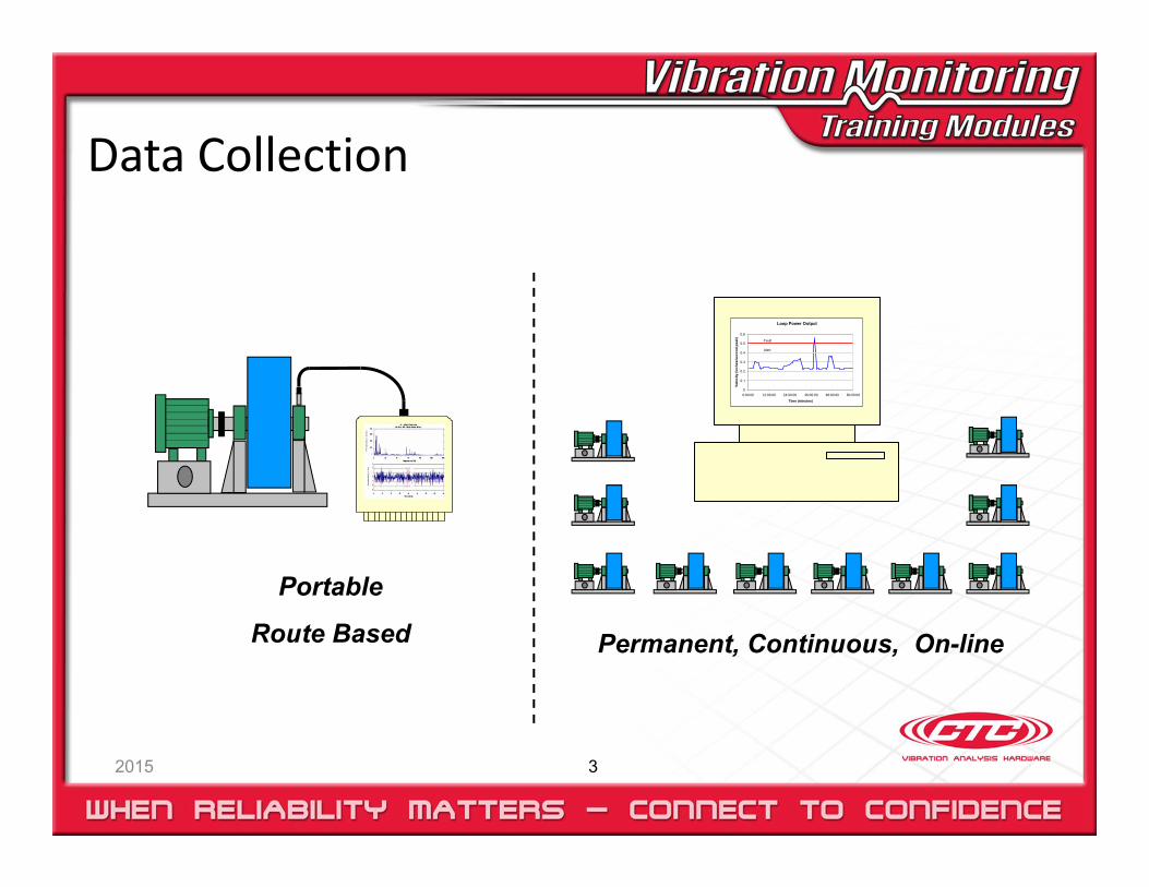
Data Collection
2015 3
Portable
Route Based Permanent, Continuous, On-line
Loop Power Output
0
0.1
0.2
0.3
0.4
0.5
0.6
0:00:00 12:00:00 24:00:00 36:00:00 48:00:00 60:00:00
Time (minutes)
Velo
city
(inc
hes/
seco
nd p
eak)
Alert
Fault

Portable Data Collectors
Route Based Frequency Spectrum Time WaveformOrbits BalancingAlignment
Data AnalysisHistory TrendingDownload DataUpload RoutesAlarms “Smart” algorithms
2015 4
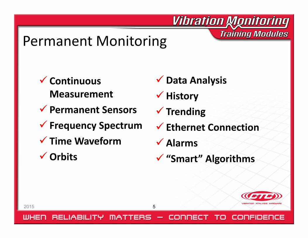
Permanent Monitoring
Continuous Measurement
Permanent Sensors Frequency Spectrum Time WaveformOrbits
Data AnalysisHistory Trending Ethernet ConnectionAlarms “Smart” Algorithms
2015 5
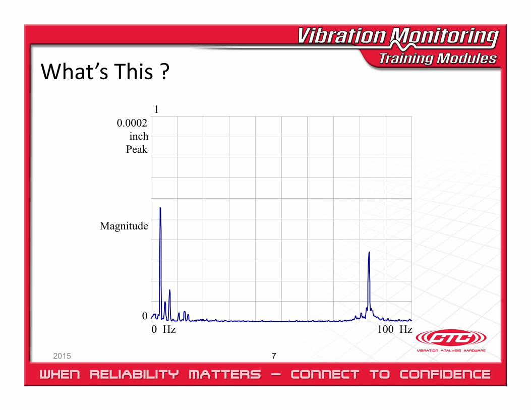
What’s This ?
2015 7
0.0002inch
Peak
0
Magnitude
Hz100 0 Hz
1
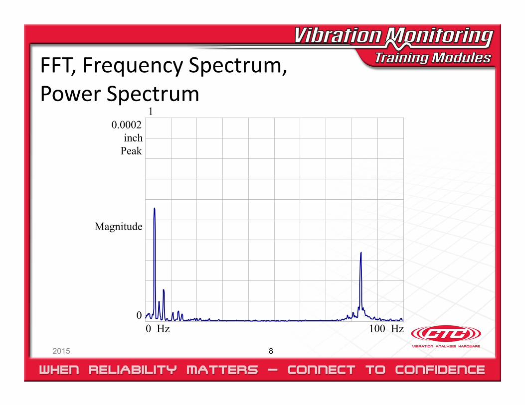
FFT, Frequency Spectrum,Power Spectrum
2015 8
0.0002inch
Peak
0
Magnitude
Hz100 0 Hz
1
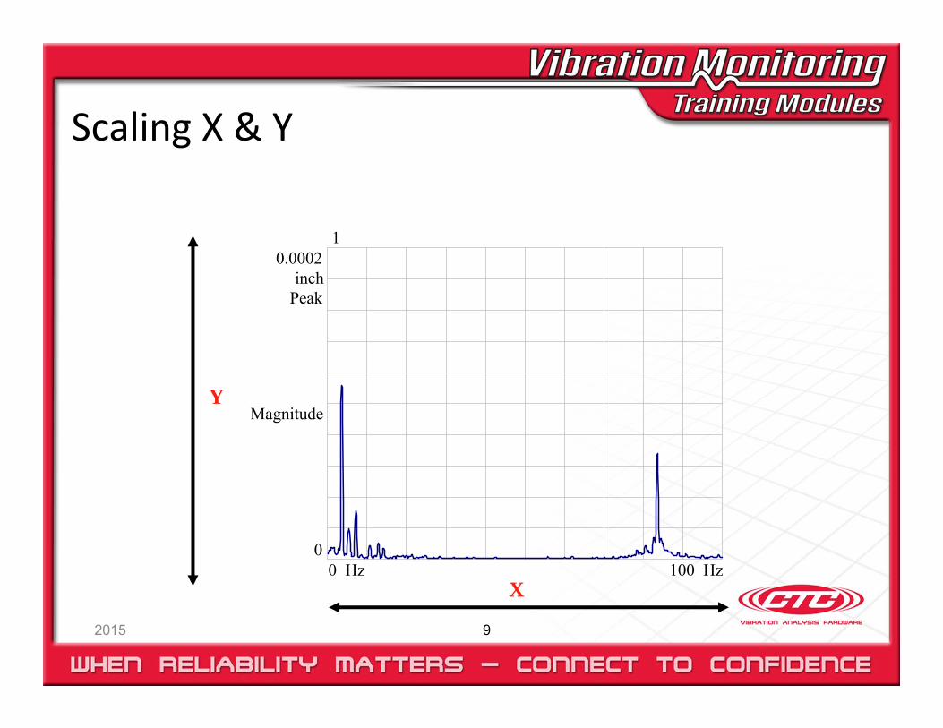
Scaling X & Y
2015 9
0.0002inch
Peak
0
Magnitude
Hz100 0 Hz
1
X
Y
Scaling X & Y
2015 10
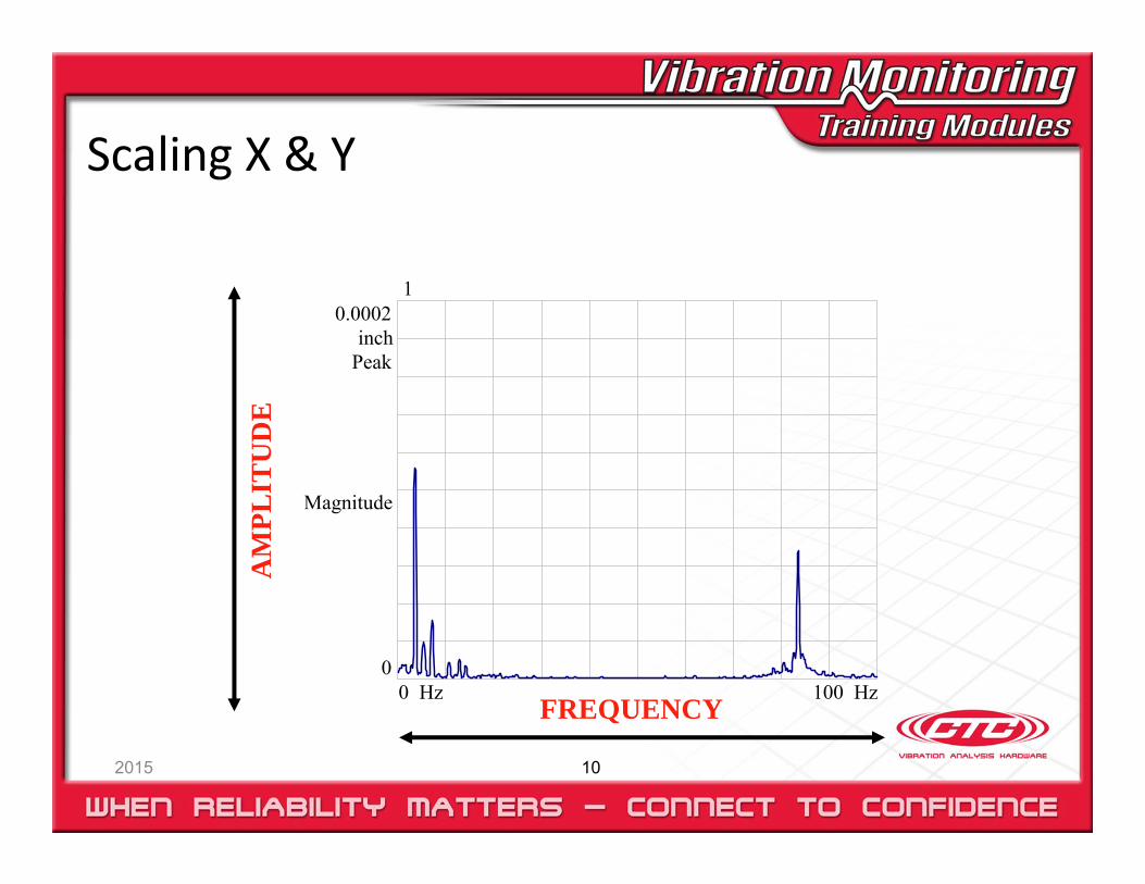
0.0002inch
Peak
0
Magnitude
Hz100 0 Hz
1
FREQUENCY
AM
PLIT
UD
E
Scaling X & Y
2015 11
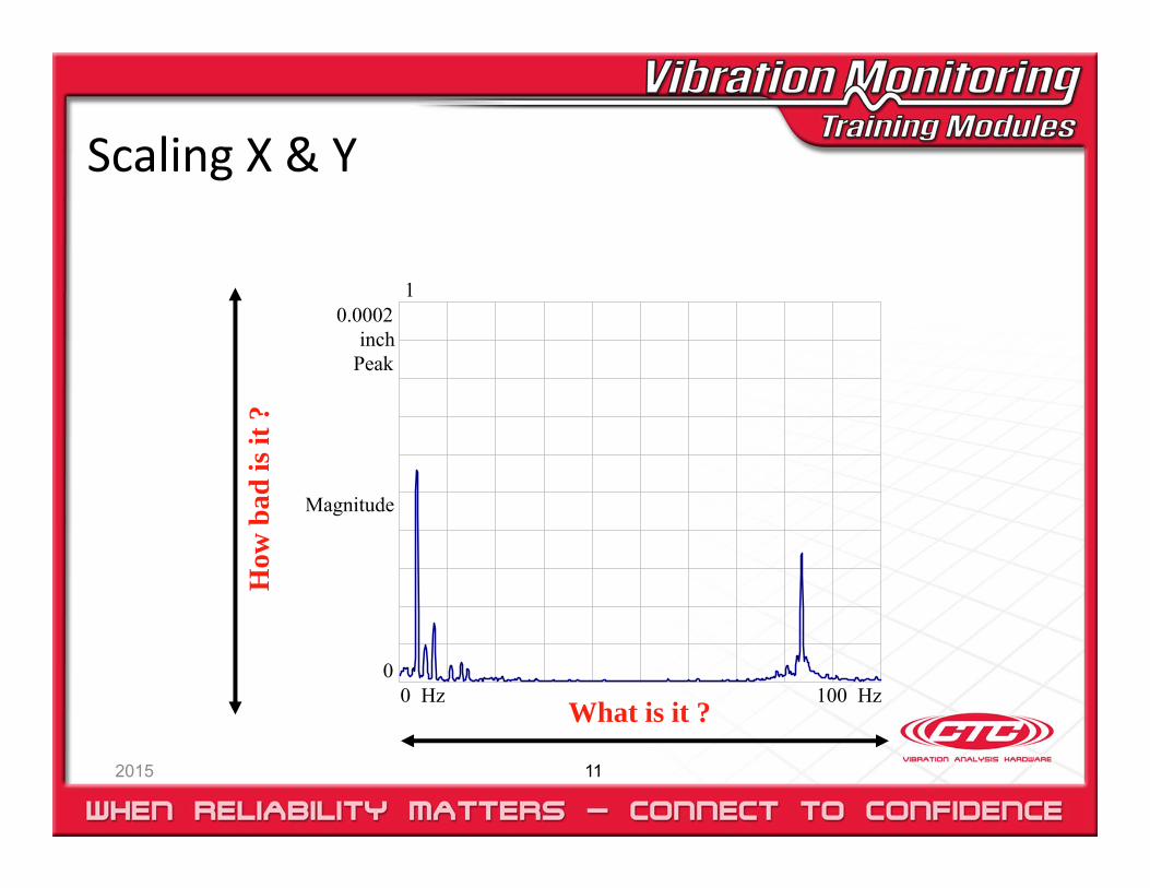
0.0002inch
Peak
0
Magnitude
Hz100 0 Hz
1
What is it ?
How
bad
is it
?
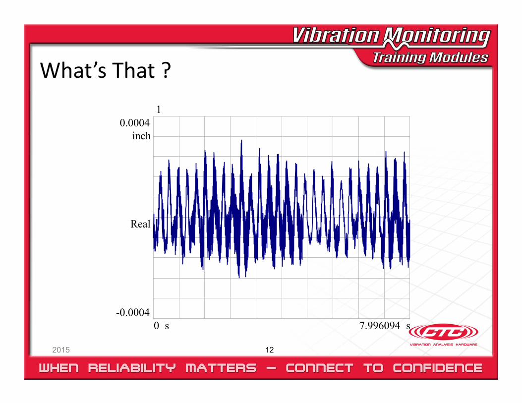
What’s That ?
2015 12
0.0004inch
-0.0004
Real
s7.996094 0 s
1
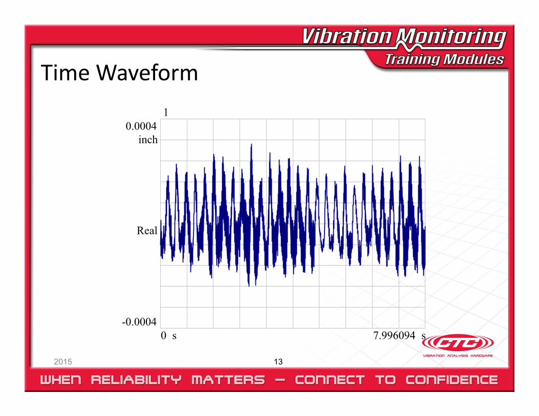
Time Waveform
2015 13
0.0004inch
-0.0004
Real
s7.996094 0 s
1
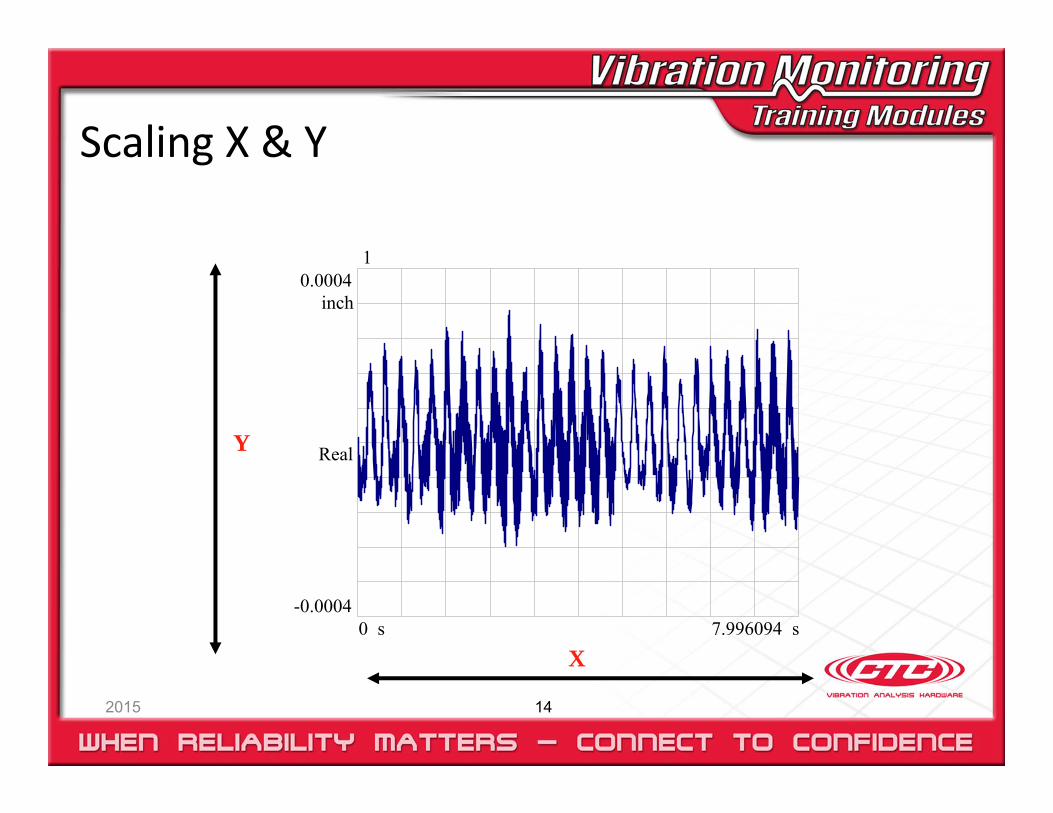
Scaling X & Y
2015 14
X
Y
0.0004inch
-0.0004
Real
s7.996094 0 s
1
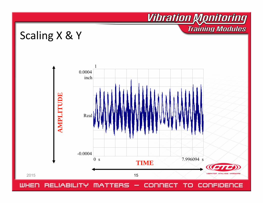
Scaling X & Y
2015 15
TIME
0.0004inch
-0.0004
Real
s7.996094 0 s
1A
MPL
ITU
DE
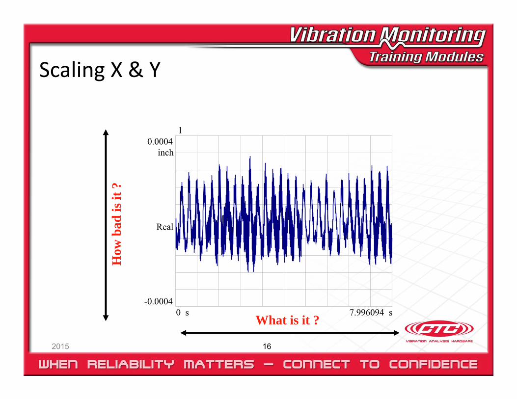
Scaling X & Y
2015 16
0.0004inch
-0.0004
Real
s7.996094 0 s
1
What is it ?
How
bad
is it
?

The X Scale
2015
What is it ?
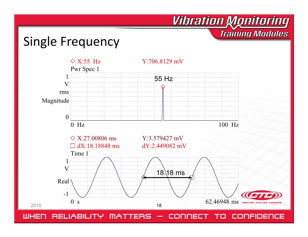
Single Frequency
2015 18
1V
rms
0
Magnitude
Hz100 0 Hz
Pwr Spec 1
1V
-1
Real
ms62.469480 s
Time 1
X:55 Hz Y:706.8129 mV
dX:18.18848 ms dY:2.449082 mVX:27.00806 ms Y:3.579427 mV
55 Hz
18.18 ms
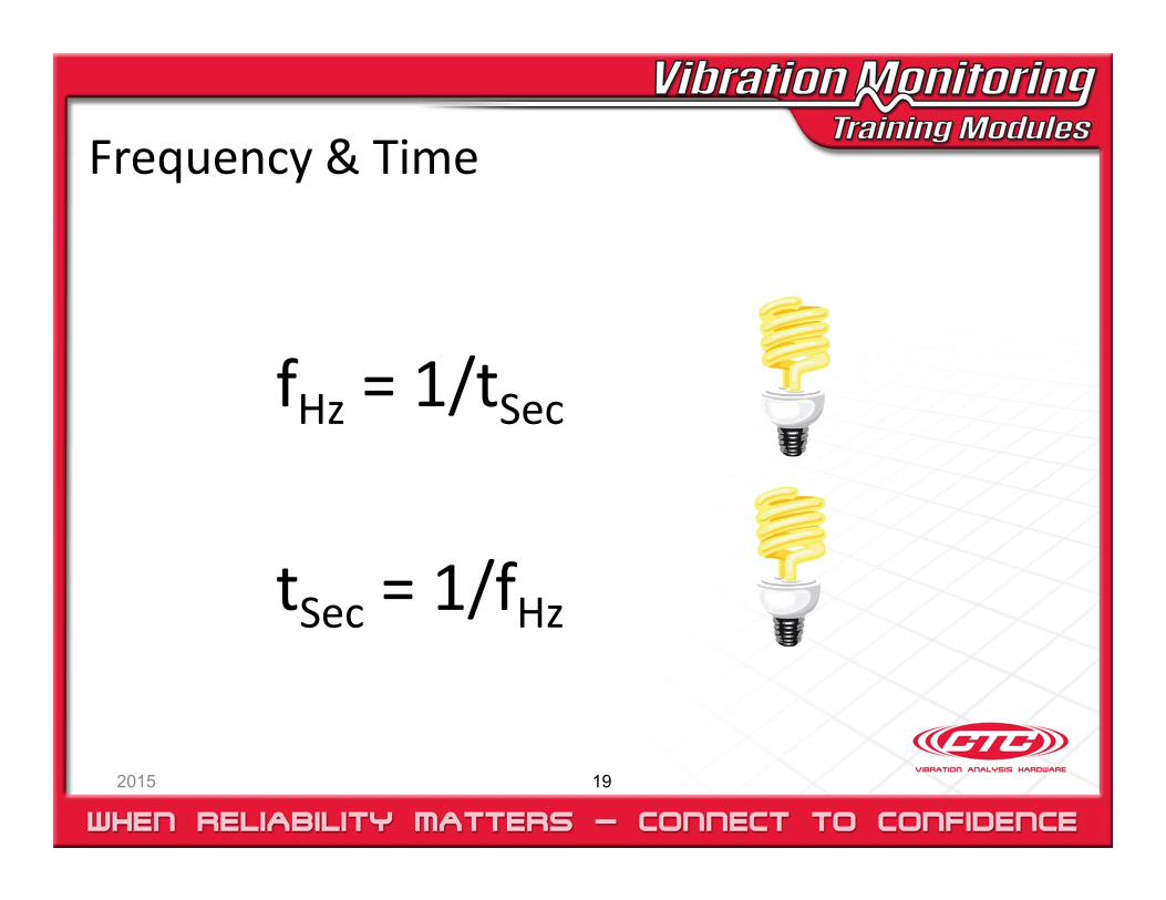
Frequency & Time
2015 19
fHz = 1/tSec
tSec = 1/fHz
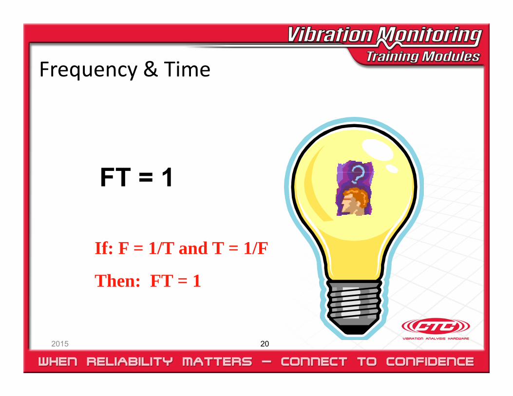
Frequency & Time
2015 20
If: F = 1/T and T = 1/F
Then: FT = 1
FT = 1
Concept !
2015 21
FT = 1
If: F increases
Then: t decreases
If: T increases
Then: f decreases
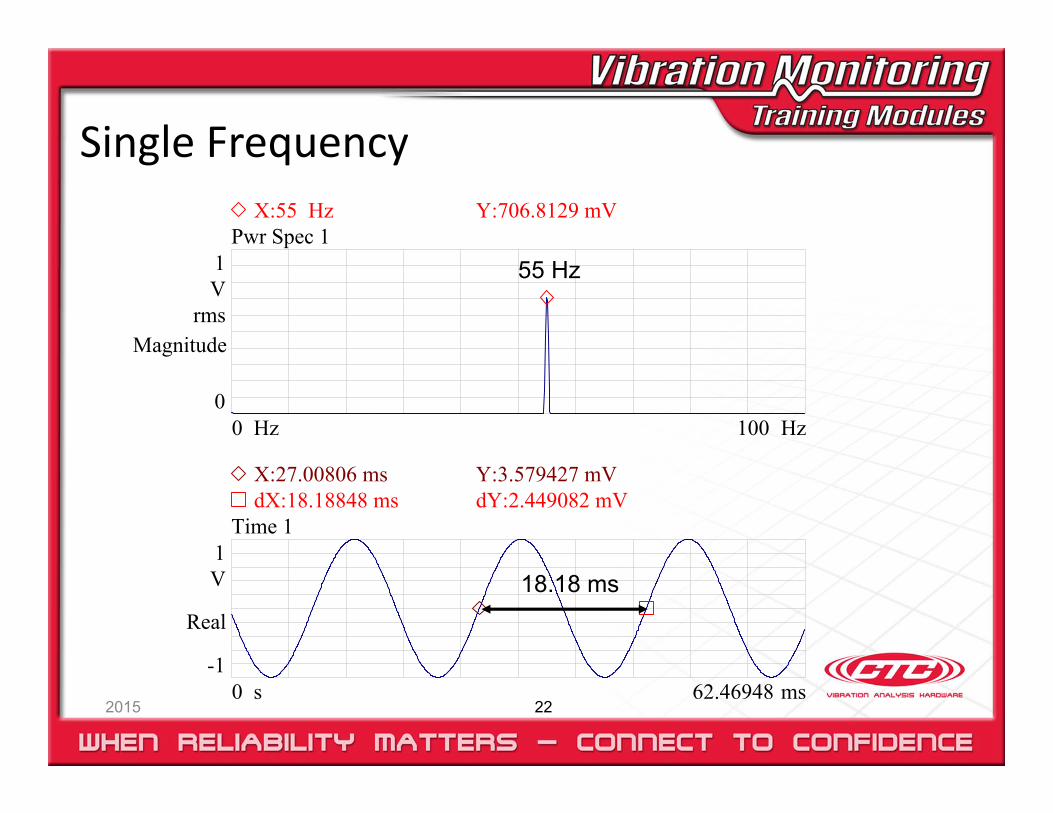
Single Frequency
2015 22
1V
rms
0
Magnitude
Hz100 0 Hz
Pwr Spec 1
1V
-1
Real
ms62.469480 s
Time 1
X:55 Hz Y:706.8129 mV
dX:18.18848 ms dY:2.449082 mVX:27.00806 ms Y:3.579427 mV
55 Hz
18.18 ms
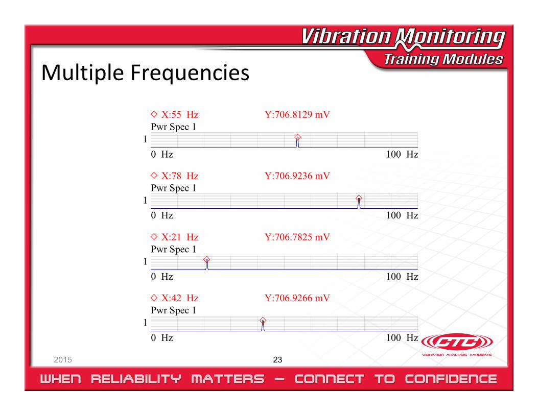
Multiple Frequencies
2015 23
1 Hz100 0 Hz
Pwr Spec 1
1 Hz100 0 Hz
Pwr Spec 1
1 Hz100 0 Hz
Pwr Spec 1
1 Hz100 0 Hz
Pwr Spec 1
X:55 Hz Y:706.8129 mV
X:78 Hz Y:706.9236 mV
X:21 Hz Y:706.7825 mV
X:42 Hz Y:706.9266 mV
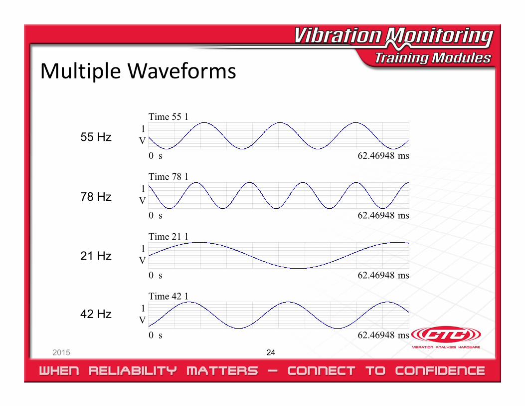
Multiple Waveforms
2015 24
1V
ms62.469480 s
Time 78 1
1V
ms62.469480 s
Time 21 1
1V
ms62.469480 s
Time 42 1
1V
ms62.469480 s
Time 55 1
55 Hz
42 Hz
21 Hz
78 Hz
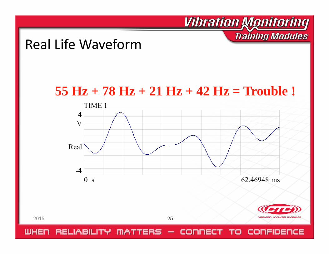
Real Life Waveform
2015 25
4V
-4
Real
ms62.469480 s
TIME 1
55 Hz + 78 Hz + 21 Hz + 42 Hz = Trouble !
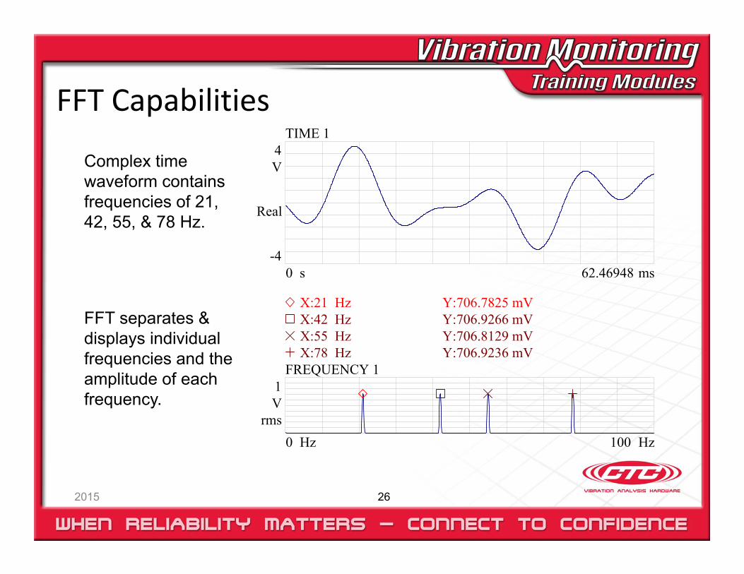
FFT Capabilities
2015 26
4V
-4
Real
ms62.469480 s
TIME 1
1V
rms Hz100 0 Hz
FREQUENCY 1X:78 Hz Y:706.9236 mVX:55 Hz Y:706.8129 mVX:42 Hz Y:706.9266 mVX:21 Hz Y:706.7825 mV
FFT separates & displays individual frequencies and the amplitude of each frequency.
Complex time waveform contains frequencies of 21, 42, 55, & 78 Hz.
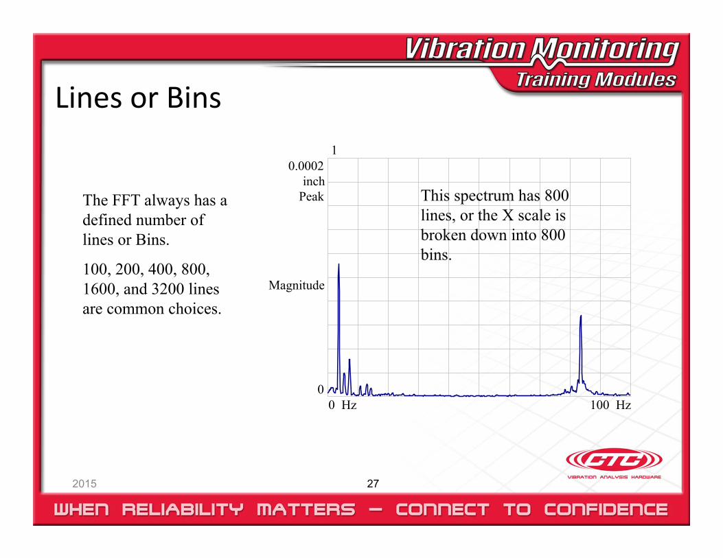
Lines or Bins
2015 27
0.0002inch
Peak
0
Magnitude
Hz100 0 Hz
1
The FFT always has a defined number of lines or Bins.
100, 200, 400, 800, 1600, and 3200 lines are common choices.
This spectrum has 800 lines, or the X scale is broken down into 800 bins.
LRF
2015 28
The Lowest Resolvable Frequency is determined by:
Frequency Span / Number of Analyzer Lines
The frequency span is calculated as the ending frequency minus the starting frequency.
The number of analyzer lines depends on the analyzer and how the operator has set it up.
Typically, this is the value that can be measured by the cursor
Example: 0 to 400 Hz using 800 lines
Answer = 400 / 800 = 0.5 Hz / Line
Bandwidth
2015 29
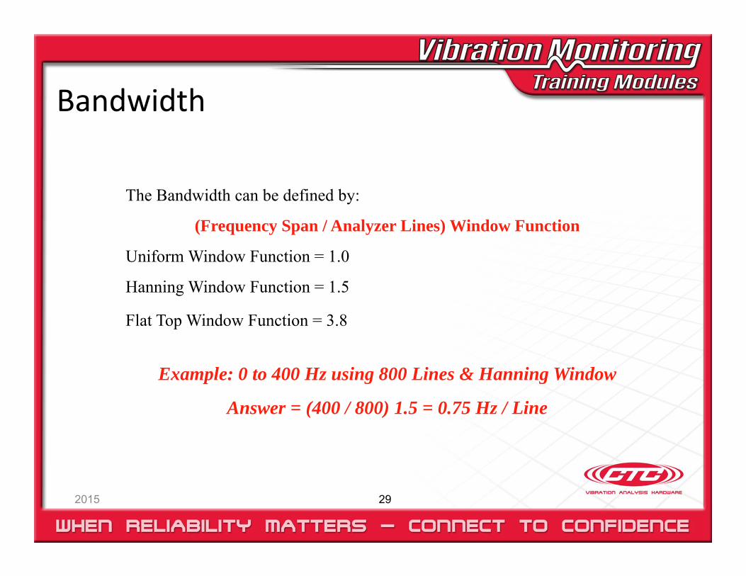
The Bandwidth can be defined by:
(Frequency Span / Analyzer Lines) Window Function
Uniform Window Function = 1.0
Hanning Window Function = 1.5
Flat Top Window Function = 3.8
Example: 0 to 400 Hz using 800 Lines & Hanning Window
Answer = (400 / 800) 1.5 = 0.75 Hz / Line
Resolution
2015 30
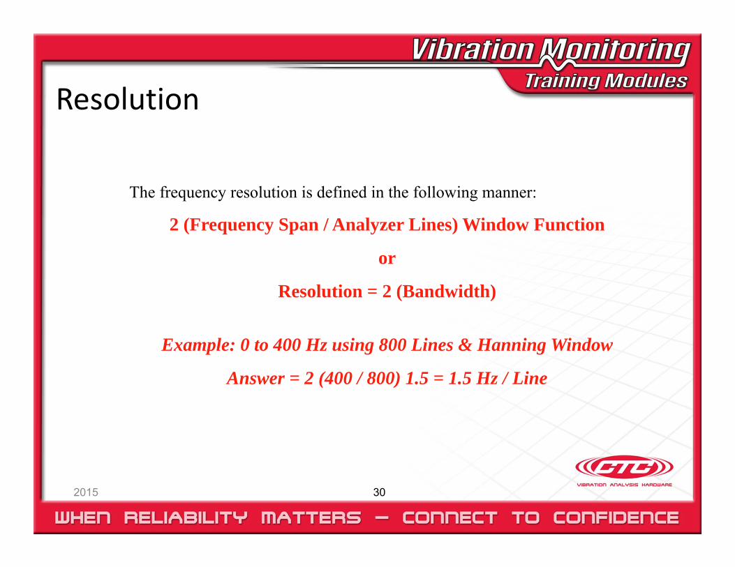
The frequency resolution is defined in the following manner:
2 (Frequency Span / Analyzer Lines) Window Function
or
Resolution = 2 (Bandwidth)
Example: 0 to 400 Hz using 800 Lines & Hanning Window
Answer = 2 (400 / 800) 1.5 = 1.5 Hz / Line
Using Resolution
2015 31
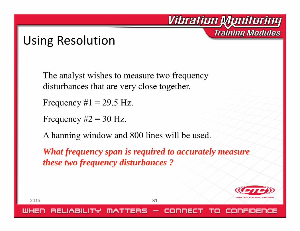
The analyst wishes to measure two frequency disturbances that are very close together.
Frequency #1 = 29.5 Hz.
Frequency #2 = 30 Hz.
A hanning window and 800 lines will be used.
What frequency span is required to accurately measure these two frequency disturbances ?
Using Resolution
2015 32
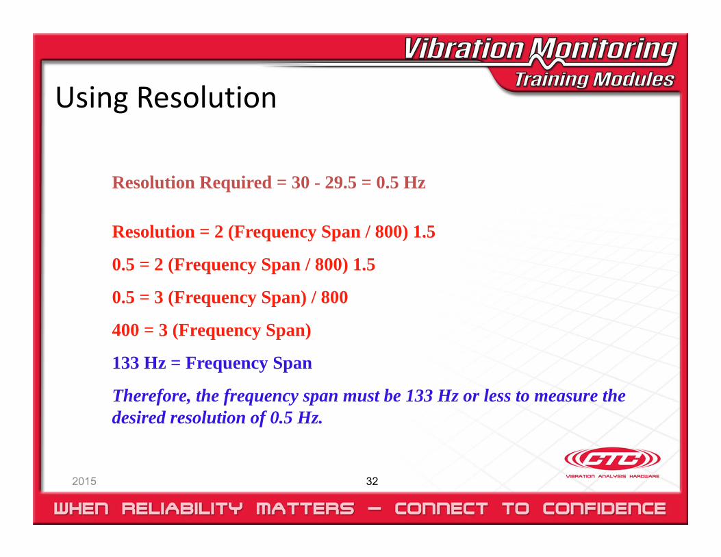
Resolution Required = 30 - 29.5 = 0.5 Hz
Resolution = 2 (Frequency Span / 800) 1.5
0.5 = 2 (Frequency Span / 800) 1.5
0.5 = 3 (Frequency Span) / 800
400 = 3 (Frequency Span)
133 Hz = Frequency Span
Therefore, the frequency span must be 133 Hz or less to measure the desired resolution of 0.5 Hz.
Data Sampling Time
2015 33
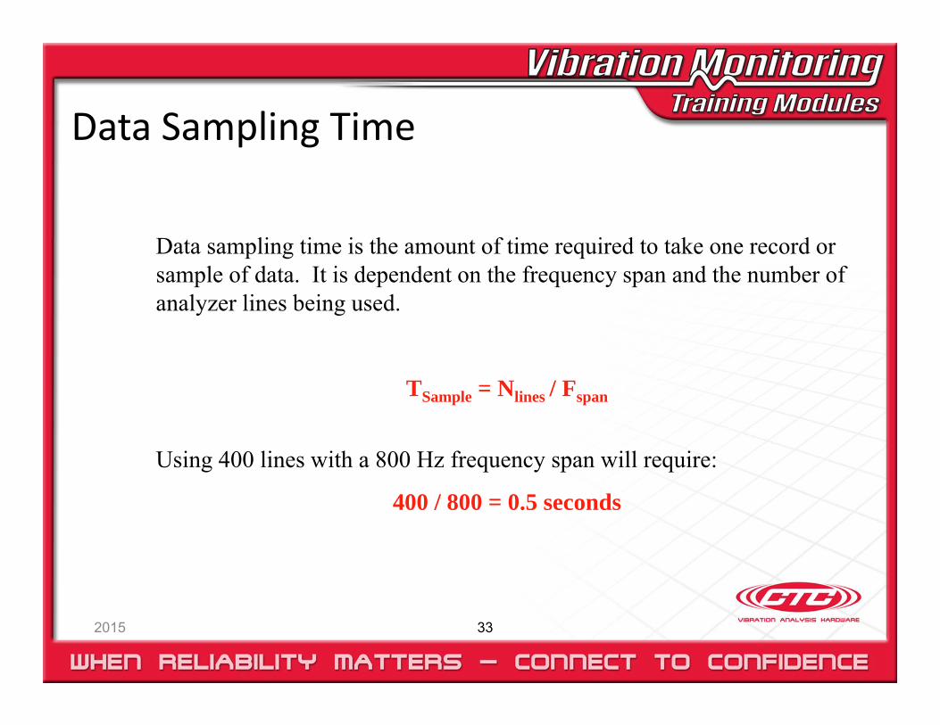
Data sampling time is the amount of time required to take one record or sample of data. It is dependent on the frequency span and the number of analyzer lines being used.
TSample = Nlines / Fspan
Using 400 lines with a 800 Hz frequency span will require:
400 / 800 = 0.5 seconds
Average & Overlap
2015 34
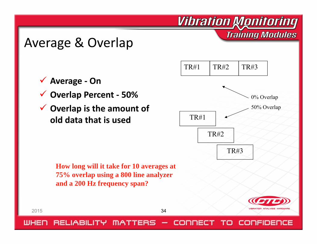
Average ‐ On Overlap Percent ‐ 50% Overlap is the amount of
old data that is used
TR#1 TR#2 TR#3
TR#1
TR#2
TR#3
0% Overlap
50% Overlap
How long will it take for 10 averages at 75% overlap using a 800 line analyzer and a 200 Hz frequency span?
75% Overlap ?
2015 35
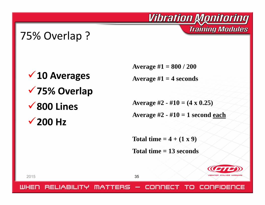
10 Averages75% Overlap800 Lines200 Hz
Average #1 = 800 / 200
Average #1 = 4 seconds
Average #2 - #10 = (4 x 0.25)
Average #2 - #10 = 1 second each
Total time = 4 + (1 x 9)
Total time = 13 seconds
Filter Windows
2015 36
Window filters are applied to the time waveform data to simulate data that starts and stops at zero.They will cause errors in the time waveform and frequency spectrum.We still like window filters !
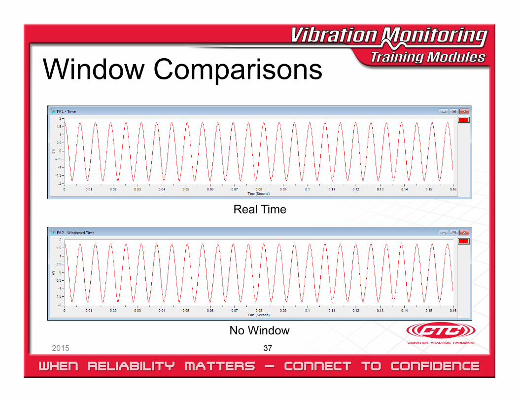
2015 37
Window Comparisons
Real Time
No Window
2015 38
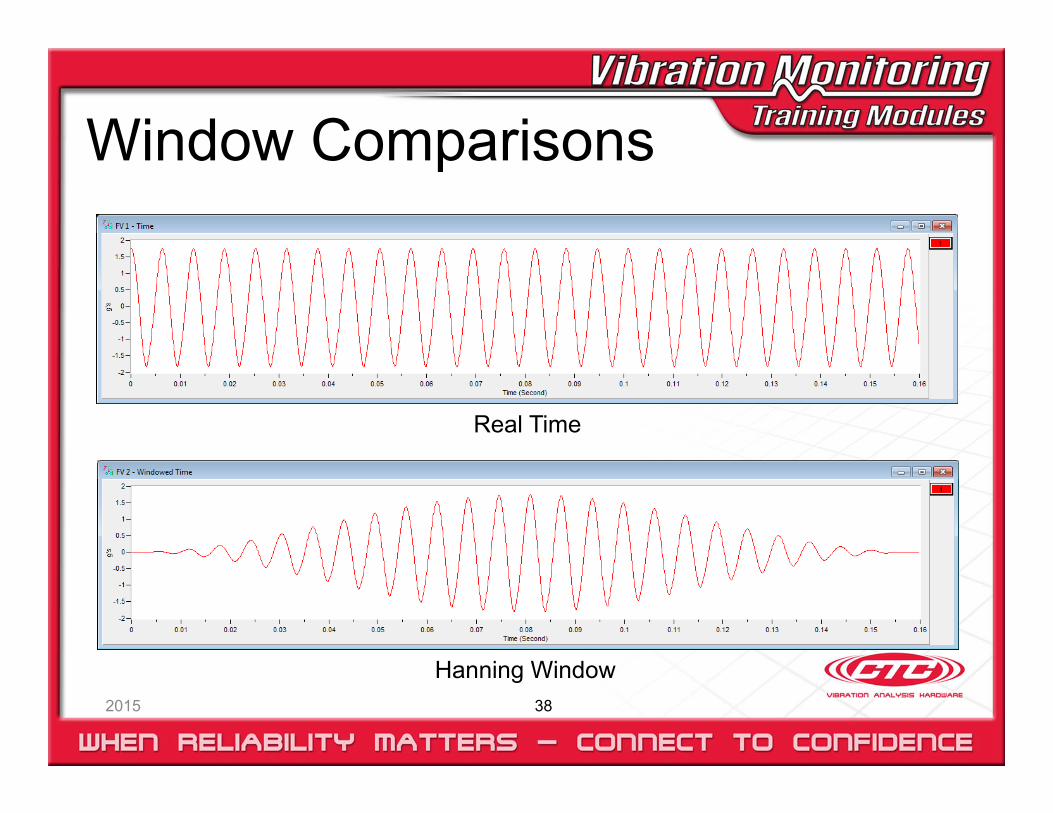
Window Comparisons
Real Time
Hanning Window
2015 39
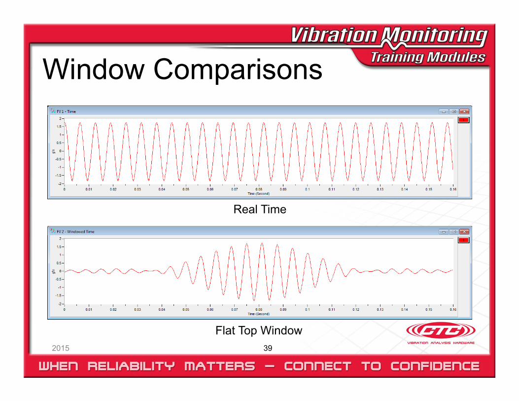
Window Comparisons
Real Time
Flat Top Window
Window Filters
2015 40
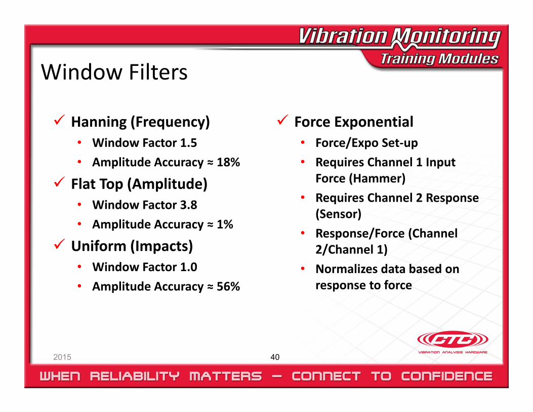
Hanning (Frequency)• Window Factor 1.5• Amplitude Accuracy ≈ 18%
Flat Top (Amplitude)• Window Factor 3.8• Amplitude Accuracy ≈ 1%
Uniform (Impacts)• Window Factor 1.0• Amplitude Accuracy ≈ 56%
Force Exponential • Force/Expo Set‐up• Requires Channel 1 Input
Force (Hammer)• Requires Channel 2 Response
(Sensor)• Response/Force (Channel
2/Channel 1)• Normalizes data based on
response to force
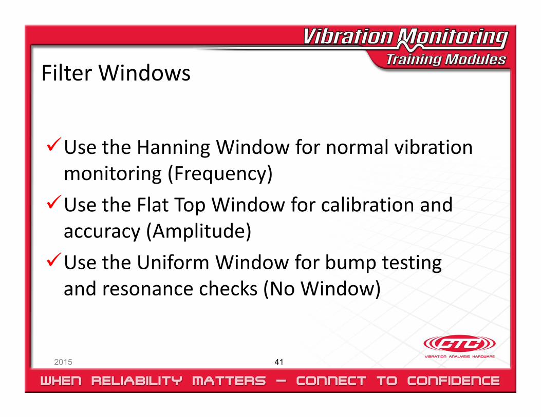
Filter Windows
2015 41
Use the Hanning Window for normal vibration monitoring (Frequency)Use the Flat Top Window for calibration and accuracy (Amplitude)Use the Uniform Window for bump testing and resonance checks (No Window)
The Y Scale
2015
How bad is it ?
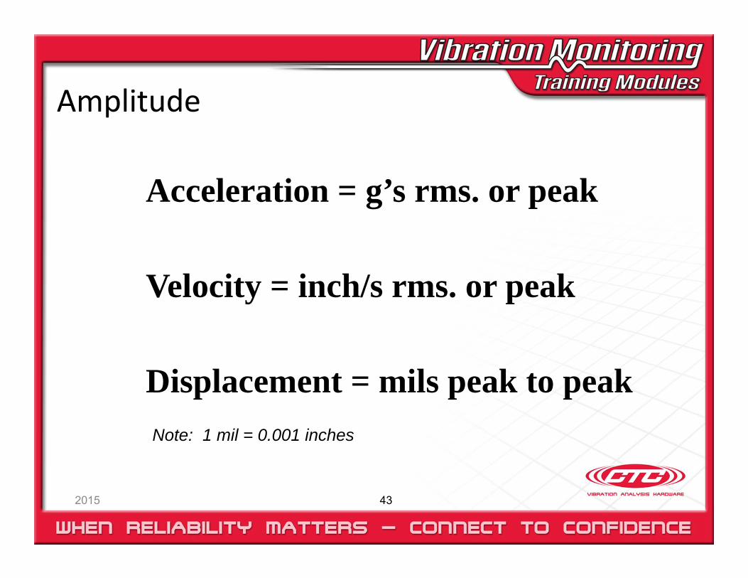
Amplitude
2015 43
Acceleration = g’s rms. or peak
Velocity = inch/s rms. or peak
Displacement = mils peak to peakNote: 1 mil = 0.001 inches
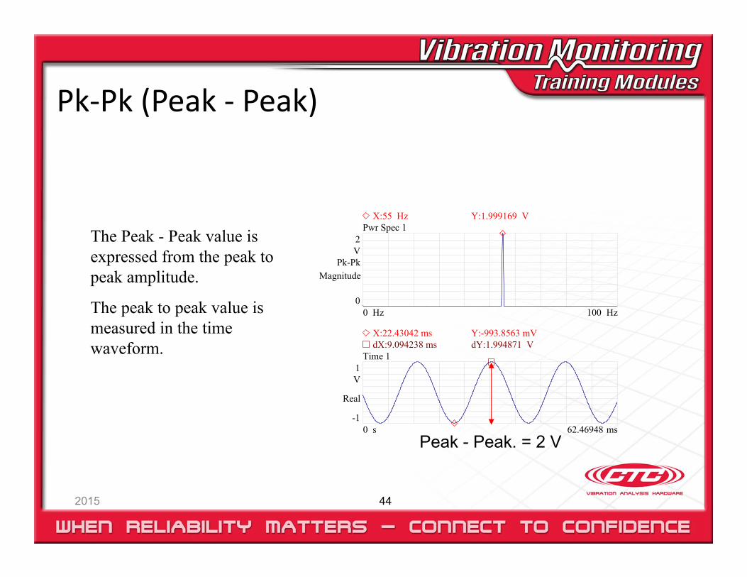
Pk‐Pk (Peak ‐ Peak)
2015 44
1V
-1
Real
ms62.469480 s
Time 1
2V
Pk-Pk
0
Magnitude
Hz100 0 Hz
Pwr Spec 1
dX:9.094238 ms dY:1.994871 VX:22.43042 ms Y:-993.8563 mV
X:55 Hz Y:1.999169 V
The Peak - Peak value is expressed from the peak to peak amplitude.
The peak to peak value is measured in the time waveform.
Peak - Peak. = 2 V
Pk (Peak)
2015 45
1V
-1
Real
ms62.469480 s
Time 1
1V
Peak
0
Magnitude
Hz100 0 Hz
Pwr Spec 1
dX:4.516602 ms dY:997.4356 mVX:27.00806 ms Y:3.579427 mV
X:55 Hz Y:999.5843 mV
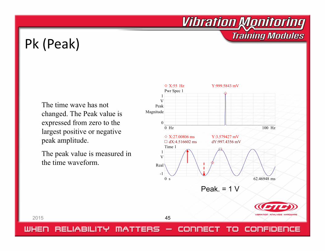
The time wave has not changed. The Peak value is expressed from zero to the largest positive or negative peak amplitude.
The peak value is measured in the time waveform.
Peak. = 1 V
RMS (Root Mean Square)
2015 46
1V
rms
0
Magnitude
Hz100 0 Hz
Pwr Spec 1
1V
-1
Real
ms62.469480 s
Time 1
X:55 Hz Y:706.8129 mV
dX:2.288818 ms dY:709.1976 mVX:27.00806 ms Y:3.579427 mV
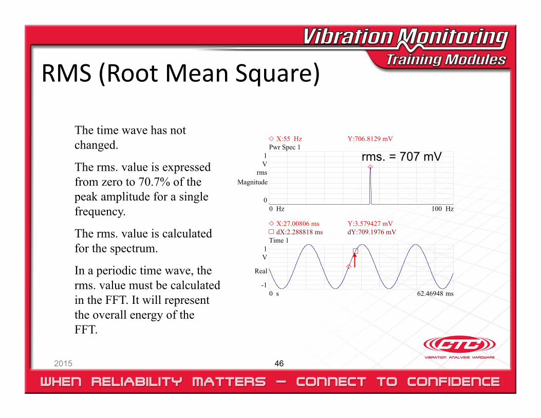
The time wave has not changed.
The rms. value is expressed from zero to 70.7% of the peak amplitude for a single frequency.
The rms. value is calculated for the spectrum.
In a periodic time wave, the rms. value must be calculated in the FFT. It will represent the overall energy of the FFT.
rms. = 707 mV
Unit Comparison
2015 47
2V
rms
0
Magnitude
Hz100 0 Hz
Pwr Spec 1
2V
Peak
0
Magnitude
Hz100 0 Hz
Pwr Spec 1
2V
Pk-Pk
0
Magnitude
Hz100 0 Hz
Pwr Spec 1
1V
-1
Real
ms62.469480 s
Time 1
1V
-1
Real
ms62.469480 s
Time 1
1V
-1
Real
ms62.469480 s
Time 1
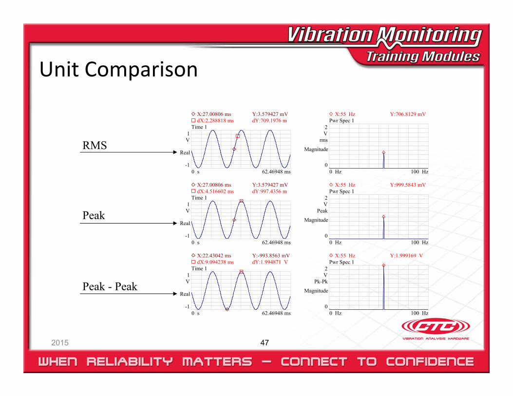
X:55 Hz Y:706.8129 mV
X:55 Hz Y:999.5843 mV
X:55 Hz Y:1.999169 V
dX:2.288818 ms dY:709.1976 mX:27.00806 ms Y:3.579427 mV
dX:4.516602 ms dY:997.4356 mX:27.00806 ms Y:3.579427 mV
dX:9.094238 ms dY:1.994871 VX:22.43042 ms Y:-993.8563 mV
RMS
Peak
Peak - Peak
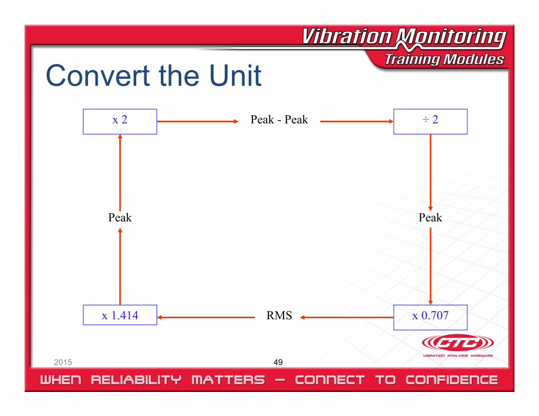
Changing Units
2015 48
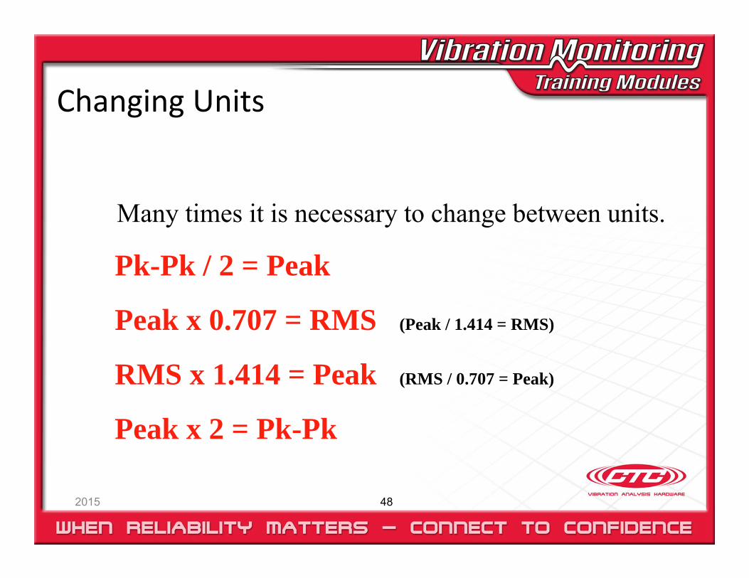
Many times it is necessary to change between units.
Pk-Pk / 2 = Peak
Peak x 0.707 = RMS (Peak / 1.414 = RMS)
RMS x 1.414 = Peak (RMS / 0.707 = Peak)
Peak x 2 = Pk-Pk
2015 49
Convert the UnitPeak - Peak
RMS
÷ 2
x 0.707
x 2
x 1.414
PeakPeak
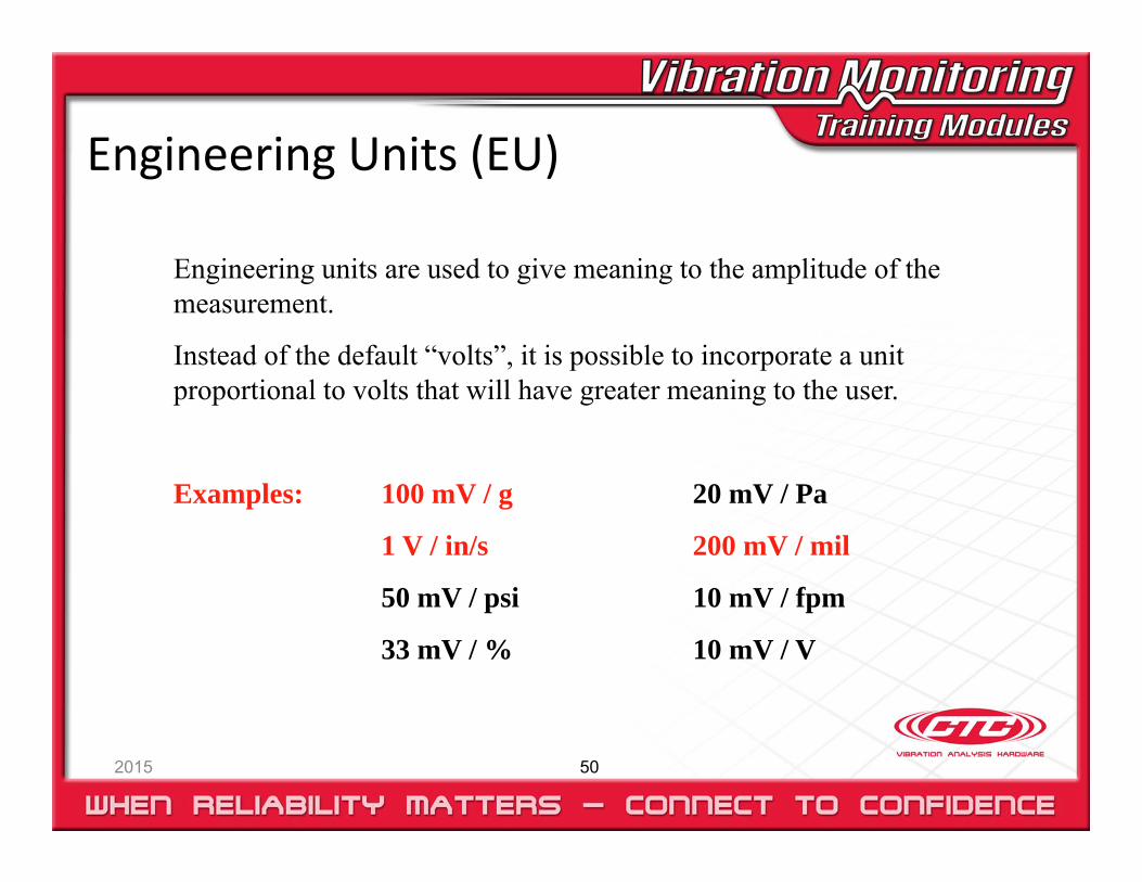
Engineering Units (EU)
2015 50
Engineering units are used to give meaning to the amplitude of the measurement.
Instead of the default “volts”, it is possible to incorporate a unit proportional to volts that will have greater meaning to the user.
Examples: 100 mV / g 20 mV / Pa
1 V / in/s 200 mV / mil
50 mV / psi 10 mV / fpm
33 mV / % 10 mV / V
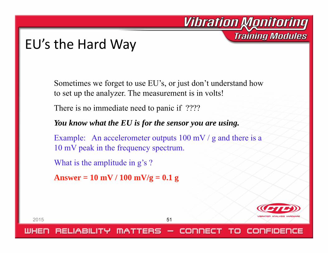
EU’s the Hard Way
2015 51
Sometimes we forget to use EU’s, or just don’t understand how to set up the analyzer. The measurement is in volts!
There is no immediate need to panic if ????
You know what the EU is for the sensor you are using.
Example: An accelerometer outputs 100 mV / g and there is a 10 mV peak in the frequency spectrum.
What is the amplitude in g’s ?
Answer = 10 mV / 100 mV/g = 0.1 g
Three Measures
2015 52
Acceleration
Velocity
Displacement

Converting Measures
2015 53
In many cases we are confronted with Acceleration, Velocity, or Displacement, but are not happy with it.
Maybe we have taken the measurement in acceleration, but the model calls for displacement.
Maybe we have taken the data in displacement, but the manufacturer quoted the equipment specifications in velocity.
How do we change between these measures ?
Converting Measures
2015 54
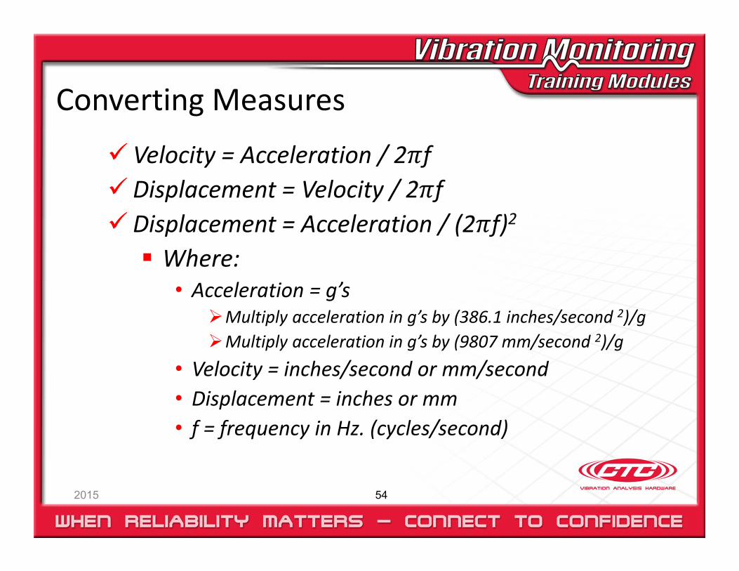
Velocity = Acceleration / 2 fDisplacement = Velocity / 2 fDisplacement = Acceleration / (2 f)2
Where:• Acceleration = g’s
Multiply acceleration in g’s by (386.1 inches/second 2)/gMultiply acceleration in g’s by (9807 mm/second 2)/g
• Velocity = inches/second or mm/second• Displacement = inches or mm• f = frequency in Hz. (cycles/second)
2015 55
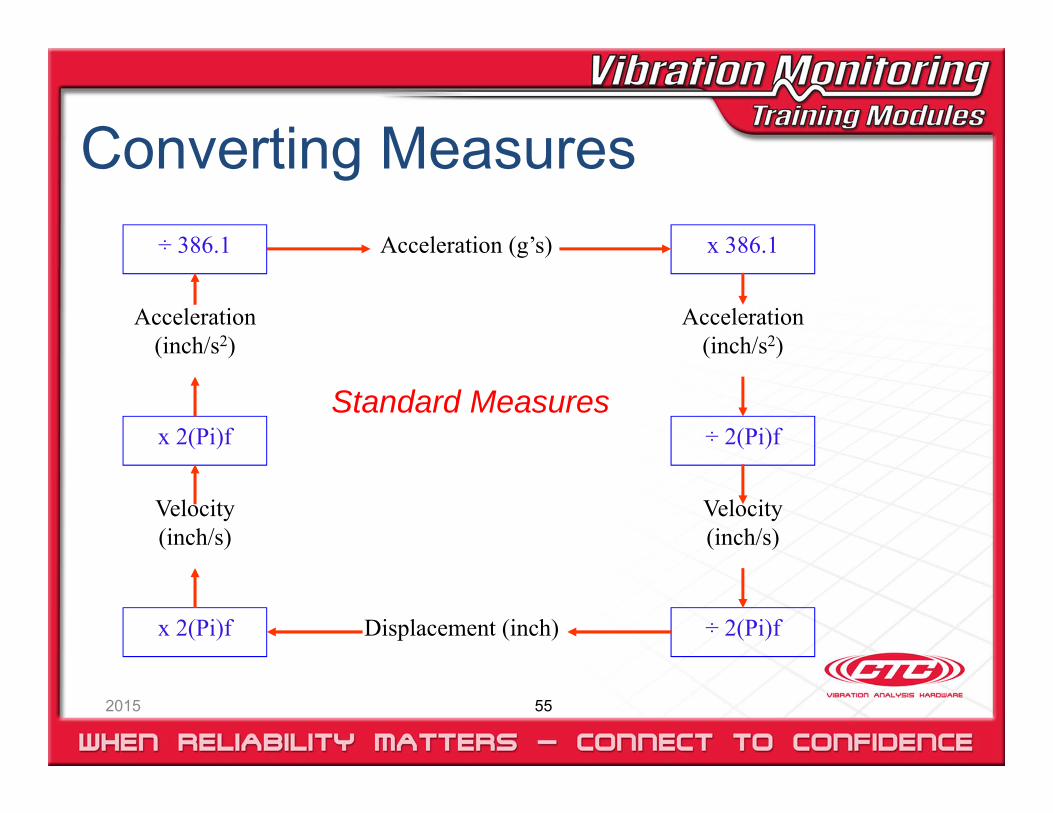
Converting MeasuresAcceleration (g’s)
Velocity (inch/s)
Displacement (inch)
x 386.1
÷ 2(Pi)f
÷ 2(Pi)fx 2(Pi)f
x 2(Pi)f
÷ 386.1
Velocity (inch/s)
Acceleration (inch/s2)
Acceleration (inch/s2)
Standard Measures
2015 56
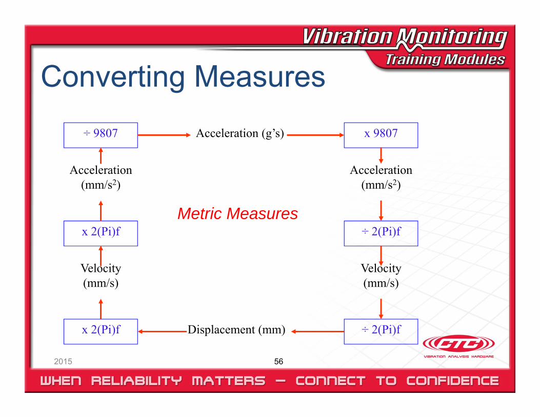
Converting Measures
Acceleration (g’s)
Velocity (mm/s)
Displacement (mm)
x 9807
÷ 2(Pi)f
÷ 2(Pi)fx 2(Pi)f
x 2(Pi)f
÷ 9807
Velocity (mm/s)
Acceleration (mm/s2)
Acceleration (mm/s2)
Metric Measures
Acceleration ‐ Velocity
2015 57
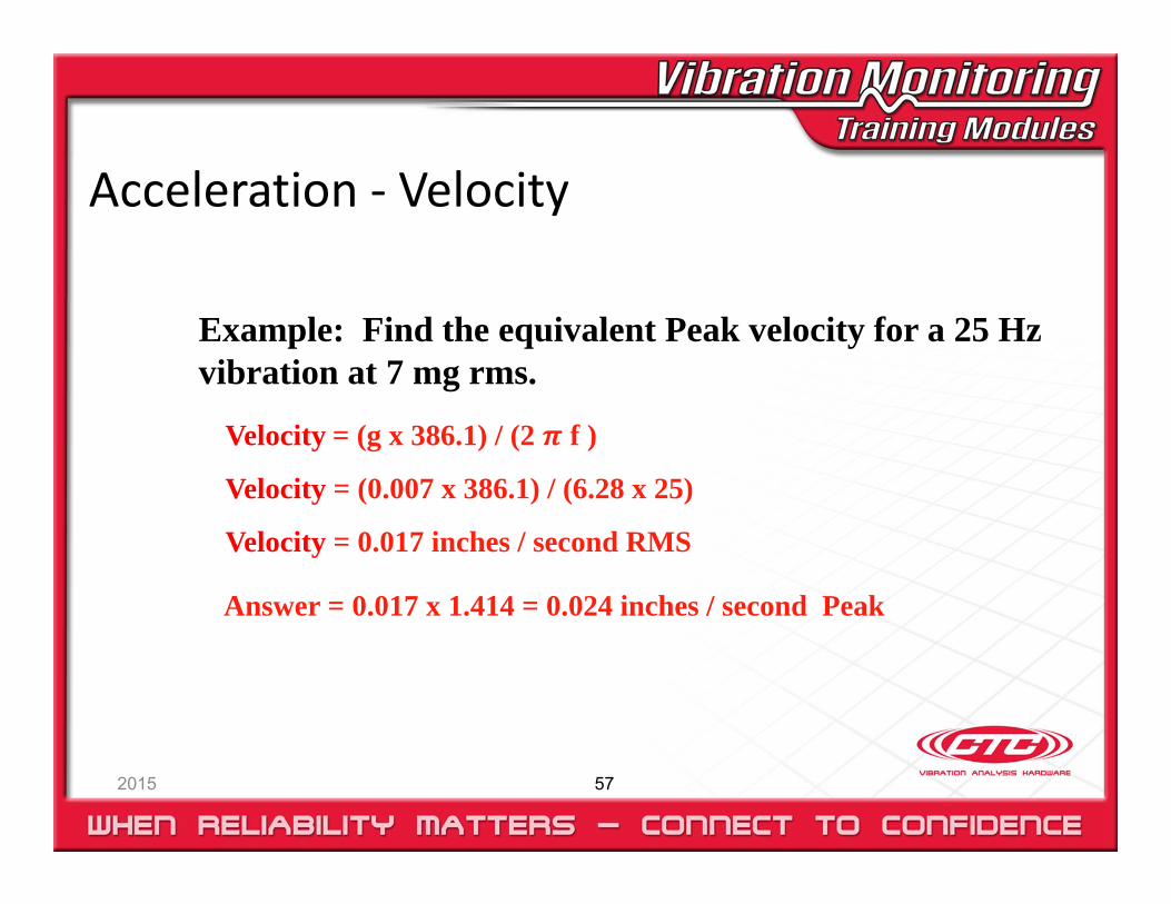
Example: Find the equivalent Peak velocity for a 25 Hz vibration at 7 mg rms.
Velocity = (g x 386.1) / (2 f )
Velocity = (0.007 x 386.1) / (6.28 x 25)
Velocity = 0.017 inches / second RMS
Answer = 0.017 x 1.414 = 0.024 inches / second Peak
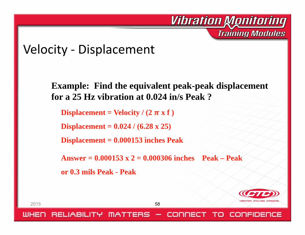
Velocity ‐ Displacement
2015 58
Example: Find the equivalent peak-peak displacement for a 25 Hz vibration at 0.024 in/s Peak ?
Displacement = Velocity / (2 x f )
Displacement = 0.024 / (6.28 x 25)
Displacement = 0.000153 inches Peak
Answer = 0.000153 x 2 = 0.000306 inches Peak – Peak
or 0.3 mils Peak - Peak
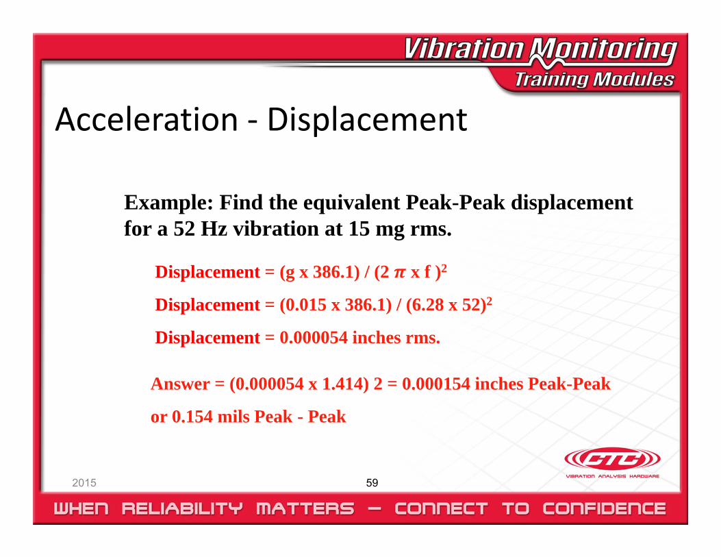
Acceleration ‐ Displacement
2015 59
Example: Find the equivalent Peak-Peak displacement for a 52 Hz vibration at 15 mg rms.
Displacement = (g x 386.1) / (2 x f )2
Displacement = (0.015 x 386.1) / (6.28 x 52)2
Displacement = 0.000054 inches rms.
Answer = (0.000054 x 1.414) 2 = 0.000154 inches Peak-Peak
or 0.154 mils Peak - Peak
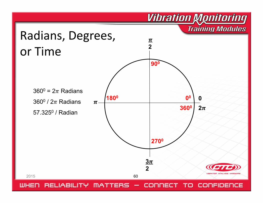
Radians, Degrees, or Time
2015 60
00
900
1800
2700
3600
2
32
2
3600 = 2 Radians
3600 / 2 Radians
57.3250 / Radian
0
2015 61
00
900
1800
2700
3600
2
32
20
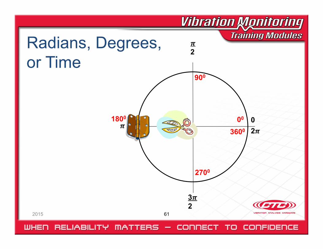
Radians, Degrees, or Time
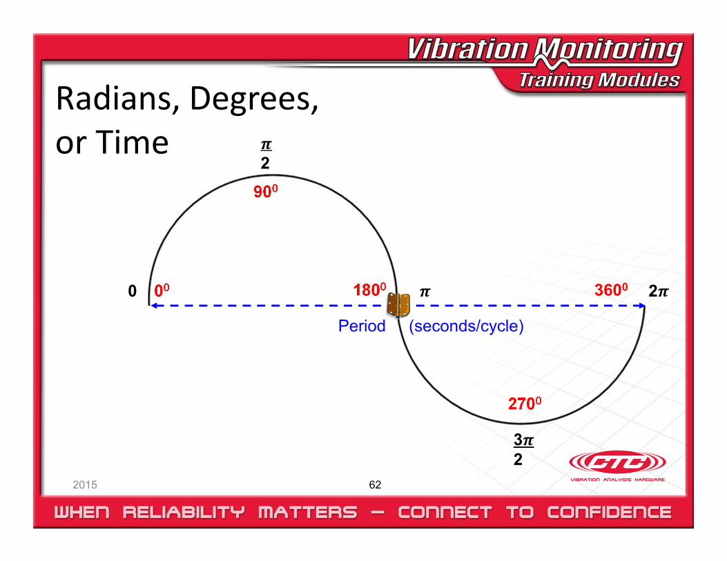
Radians, Degrees, or Time
2015 62
00
900
1800
2700
3600
2
32
2
Period (seconds/cycle)
0
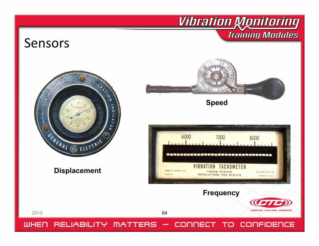
Sensors
2015 64
Displacement
Frequency
Speed

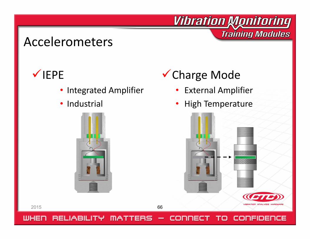
Accelerometers
2015 66
IEPE• Integrated Amplifier• Industrial
Charge Mode• External Amplifier• High Temperature
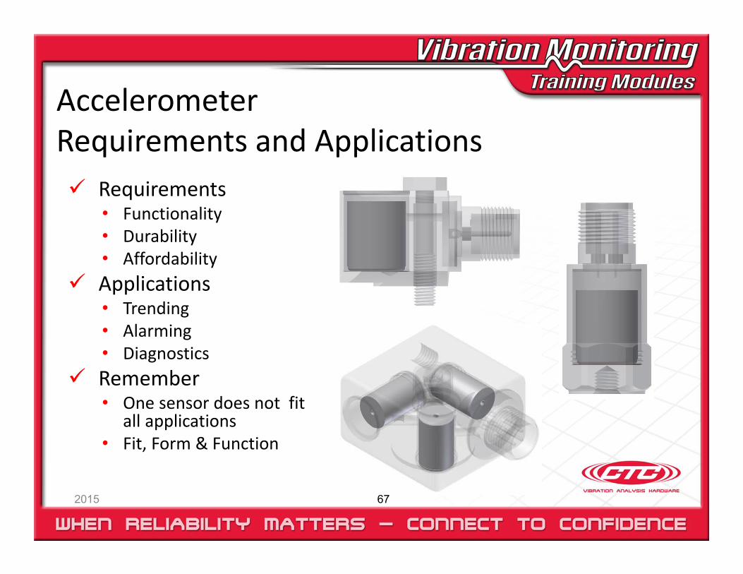
AccelerometerRequirements and Applications
2015 67
Requirements• Functionality• Durability• Affordability
Applications• Trending• Alarming• Diagnostics
Remember• One sensor does not fit
all applications• Fit, Form & Function
Accelerometer Advantages
2015 68
Measures casing vibrationMeasures absolute vibrationIntegrate to VelocityDouble integrate to Displacement Easy to mountLarge range of frequency responseAvailable in many configurations
Accelerometer Disadvantages
2015 69
Does not measure shaft vibrationSensitive to mounting techniques and surface conditionsDifficult to perform calibration checkOne accelerometer does not fit all applications
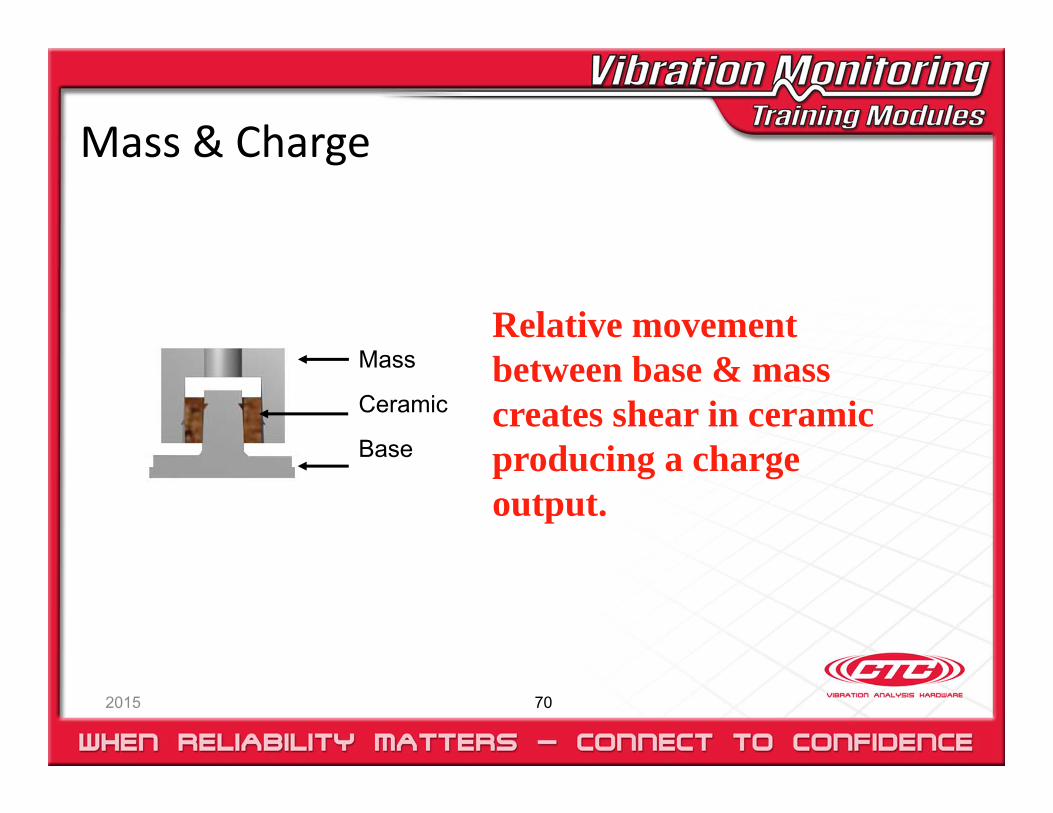
Mass & Charge
2015 70
Relative movement between base & mass creates shear in ceramic producing a charge output.
Mass
Ceramic
Base
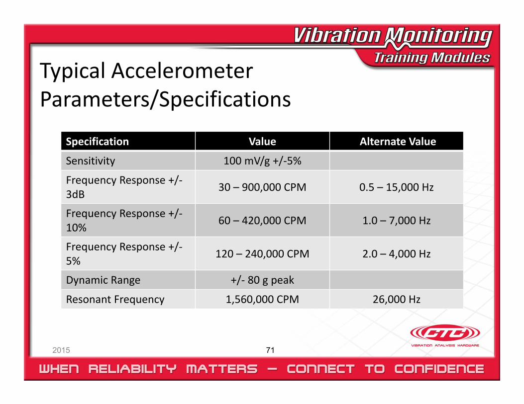
Typical Accelerometer Parameters/Specifications
2015 71
Specification Value Alternate Value
Sensitivity 100 mV/g +/‐5%
Frequency Response +/‐3dB 30 – 900,000 CPM 0.5 – 15,000 Hz
Frequency Response +/‐10% 60 – 420,000 CPM 1.0 – 7,000 Hz
Frequency Response +/‐5% 120 – 240,000 CPM 2.0 – 4,000 Hz
Dynamic Range +/‐ 80 g peak
Resonant Frequency 1,560,000 CPM 26,000 Hz
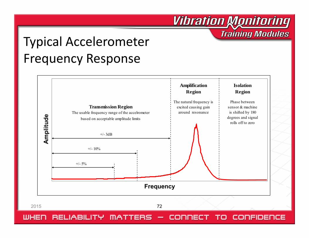
Typical AccelerometerFrequency Response
2015 72
Frequency
Am
plitu
de
+/- 3dB
+/- 10%
Transmission RegionThe usable frequency range of the accelrometer
based on acceptable amplitude limits
AmplificationRegion
The natural frequency is excited causing gain around resonance
IsolationRegion
Phase between sensor & machine is shifted by 180
degrees and signal rolls off to zero
+/- 5%
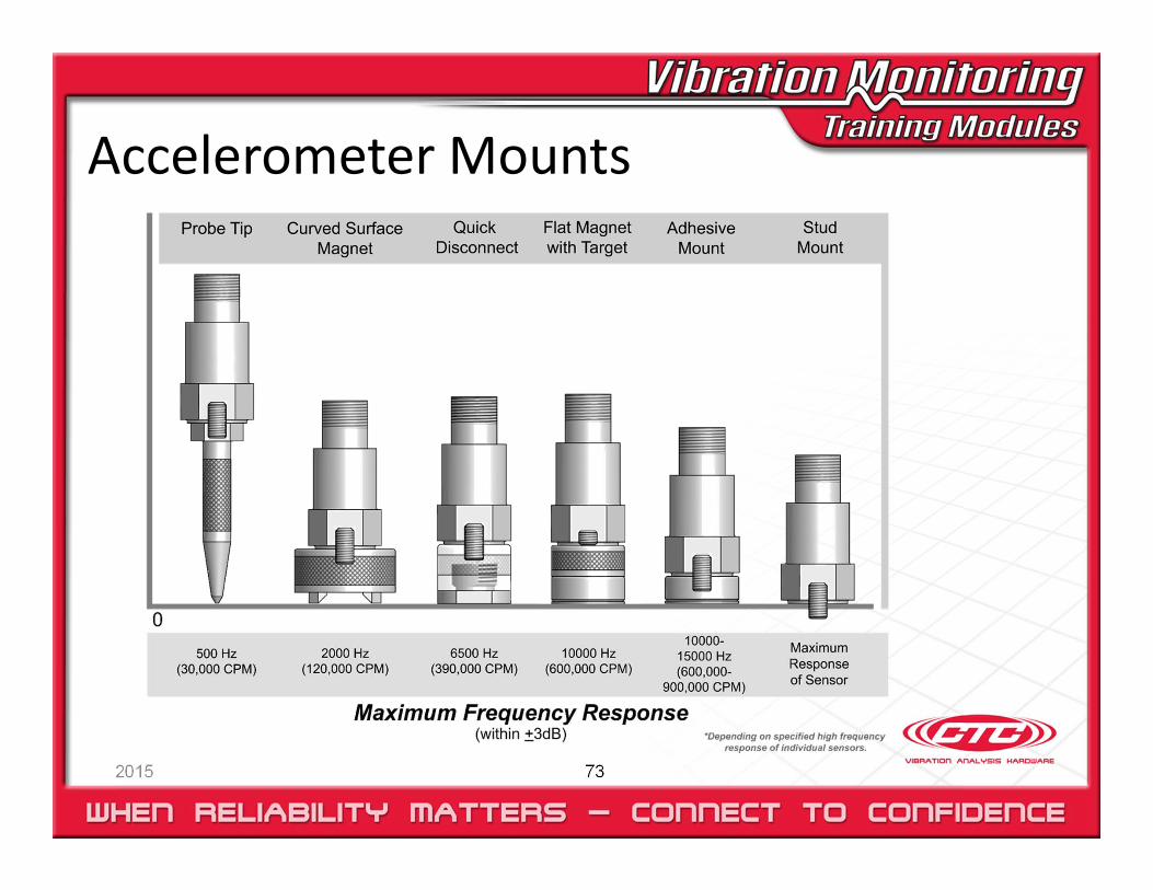
Accelerometer Mounts
2015 73
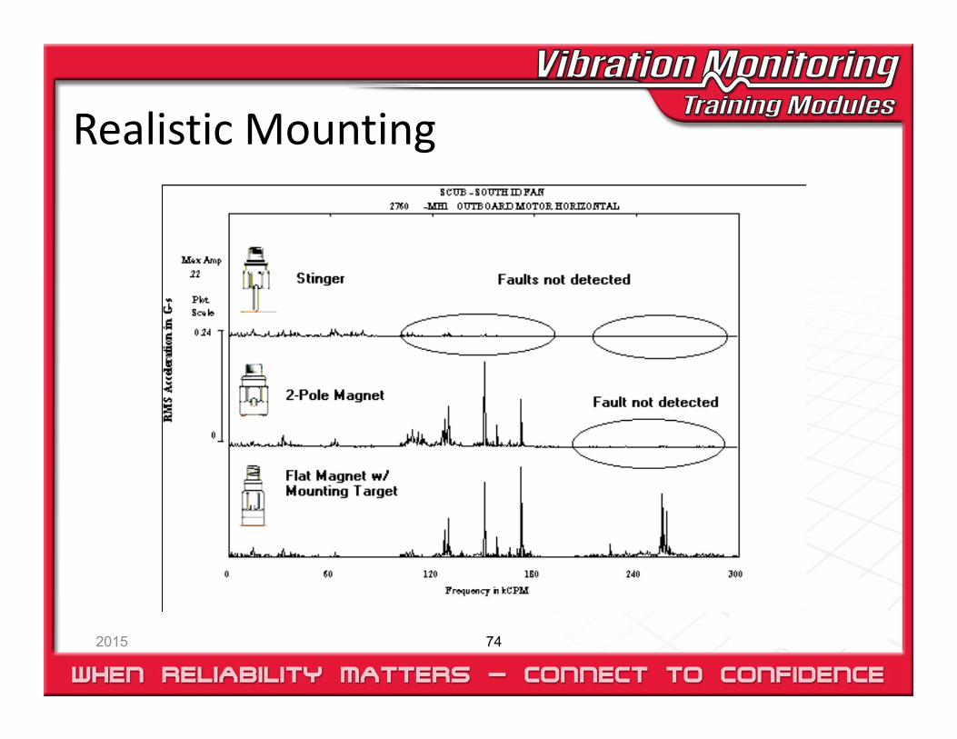
Realistic Mounting
2015 74
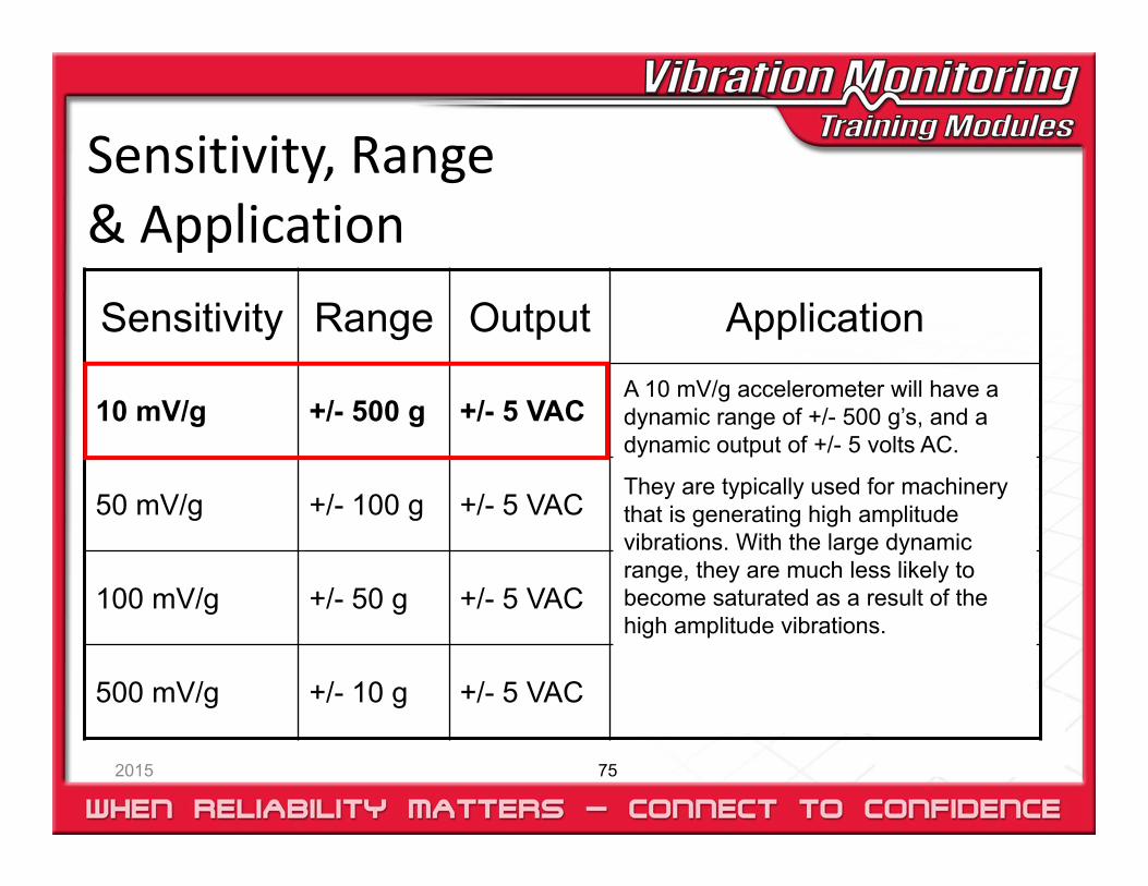
Sensitivity, Range & Application
2015 75
Sensitivity Range Output Application
10 mV/g +/- 500 g +/- 5 VAC
50 mV/g +/- 100 g +/- 5 VAC
100 mV/g +/- 50 g +/- 5 VAC
500 mV/g +/- 10 g +/- 5 VAC
A 10 mV/g accelerometer will have a dynamic range of +/- 500 g’s, and a dynamic output of +/- 5 volts AC.
They are typically used for machinery that is generating high amplitude vibrations. With the large dynamic range, they are much less likely to become saturated as a result of the high amplitude vibrations.
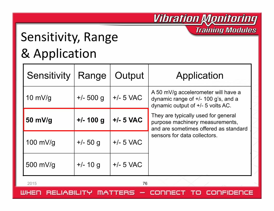
Sensitivity, Range & Application
2015 76
Sensitivity Range Output Application
10 mV/g +/- 500 g +/- 5 VAC
50 mV/g +/- 100 g +/- 5 VAC
100 mV/g +/- 50 g +/- 5 VAC
500 mV/g +/- 10 g +/- 5 VAC
A 50 mV/g accelerometer will have a dynamic range of +/- 100 g’s, and a dynamic output of +/- 5 volts AC.
They are typically used for general purpose machinery measurements, and are sometimes offered as standard sensors for data collectors.
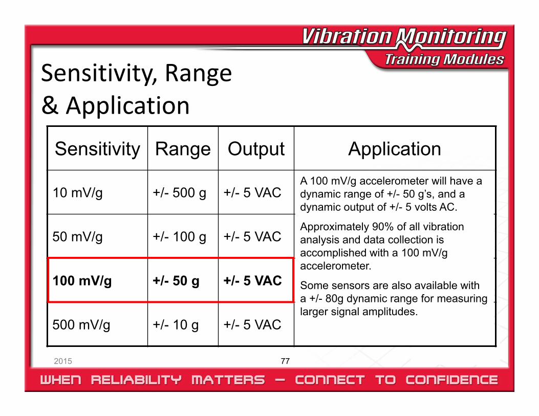
Sensitivity, Range & Application
2015 77
Sensitivity Range Output Application
10 mV/g +/- 500 g +/- 5 VAC
50 mV/g +/- 100 g +/- 5 VAC
100 mV/g +/- 50 g +/- 5 VAC
500 mV/g +/- 10 g +/- 5 VAC
A 100 mV/g accelerometer will have a dynamic range of +/- 50 g’s, and a dynamic output of +/- 5 volts AC.
Approximately 90% of all vibration analysis and data collection is accomplished with a 100 mV/g accelerometer.
Some sensors are also available with a +/- 80g dynamic range for measuring larger signal amplitudes.
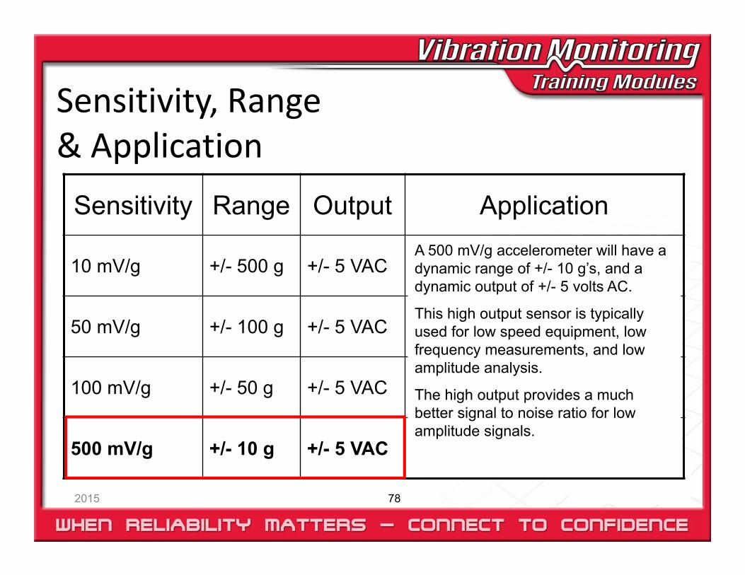
Sensitivity, Range & Application
2015 78
Sensitivity Range Output Application
10 mV/g +/- 500 g +/- 5 VAC
50 mV/g +/- 100 g +/- 5 VAC
100 mV/g +/- 50 g +/- 5 VAC
500 mV/g +/- 10 g +/- 5 VAC
A 500 mV/g accelerometer will have a dynamic range of +/- 10 g’s, and a dynamic output of +/- 5 volts AC.
This high output sensor is typically used for low speed equipment, low frequency measurements, and low amplitude analysis.
The high output provides a much better signal to noise ratio for low amplitude signals.
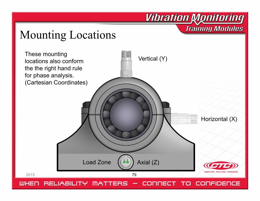
Mounting Locations
2015 79
Load Zone Axial (Z)
Horizontal (X)
Vertical (Y)These mounting locations also conform the the right hand rule for phase analysis. (Cartesian Coordinates)
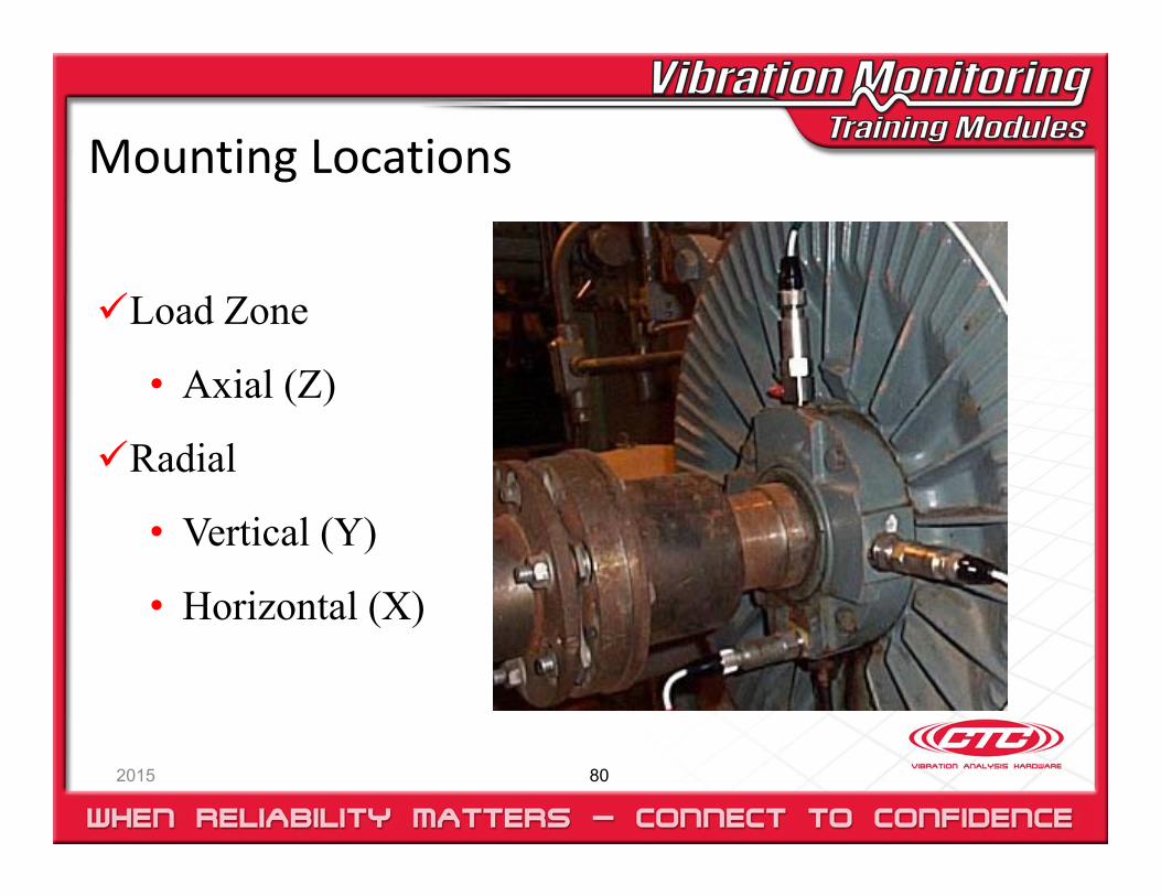
Mounting Locations
2015 80
Load Zone
• Axial (Z)
Radial
• Vertical (Y)
• Horizontal (X)

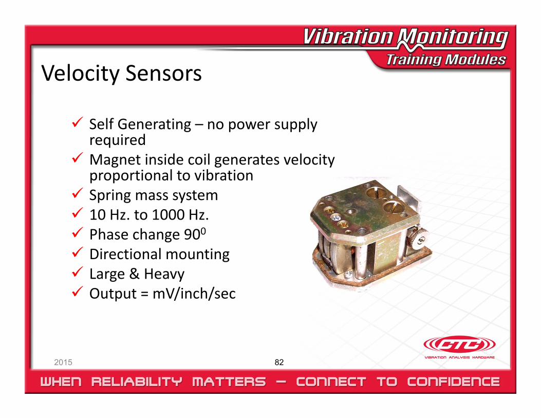
Velocity Sensors
2015 82
Self Generating – no power supply required
Magnet inside coil generates velocity proportional to vibration
Spring mass system 10 Hz. to 1000 Hz. Phase change 900 Directional mounting Large & Heavy Output = mV/inch/sec
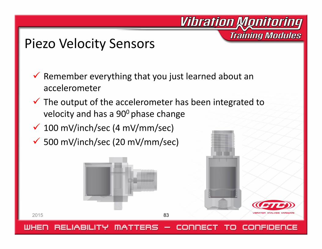
Piezo Velocity Sensors
2015 83
Remember everything that you just learned about an accelerometer
The output of the accelerometer has been integrated to velocity and has a 900 phase change
100 mV/inch/sec (4 mV/mm/sec) 500 mV/inch/sec (20 mV/mm/sec)

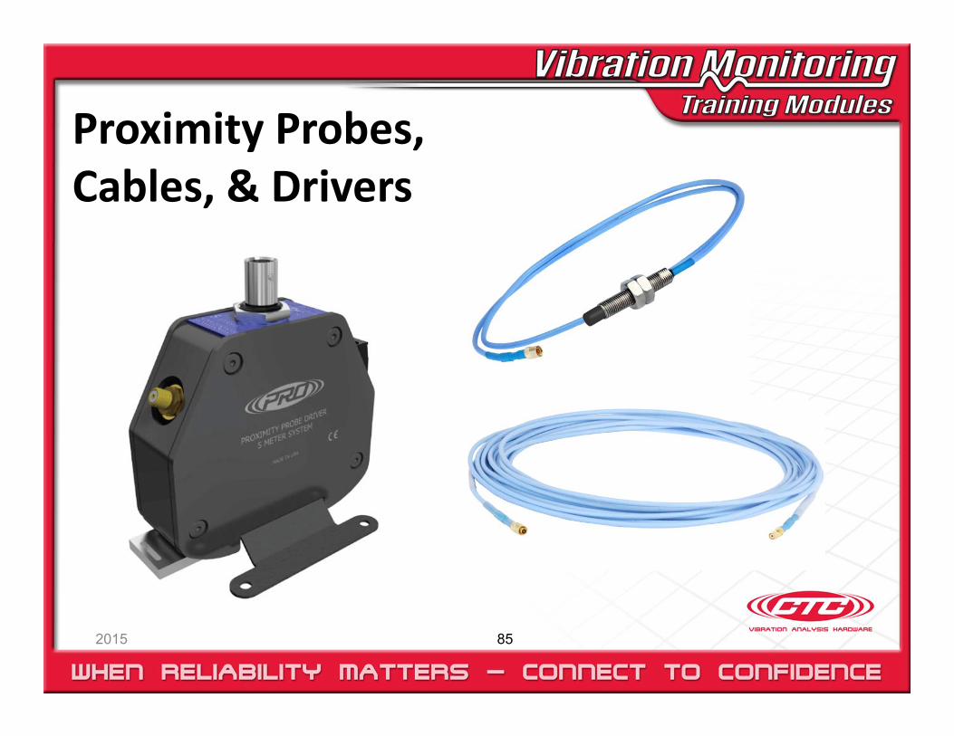
Proximity Probes, Cables, & Drivers
2015 85
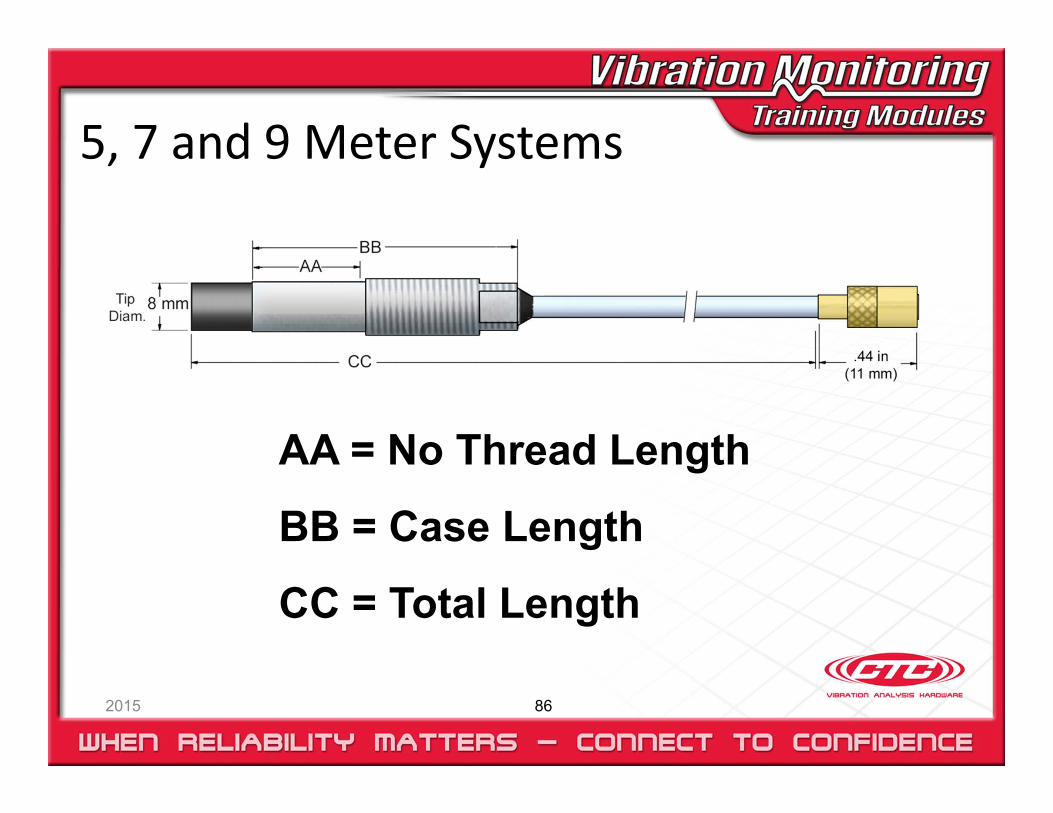
5, 7 and 9 Meter Systems
2015 86
AA = No Thread Length
BB = Case Length
CC = Total Length

5, 7 & 9 Meter Systems
2015 87
Probe Length + Extension Cable Length
must equal 5, 7 or 9 meters in system length
Extension Cable
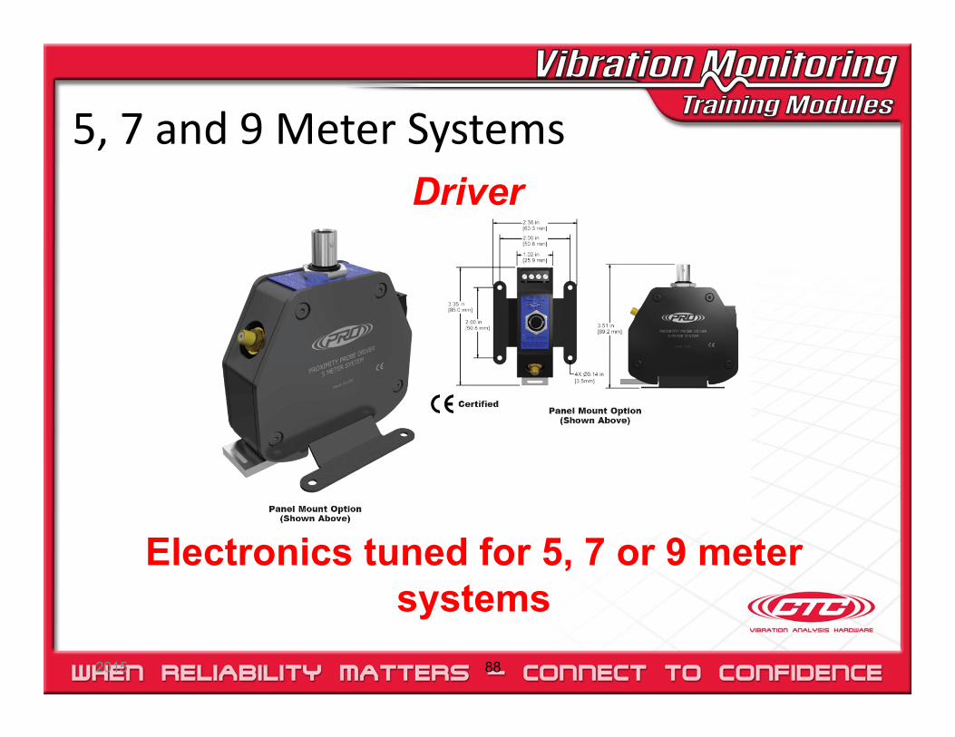
5, 7 and 9 Meter Systems
2015 88
Electronics tuned for 5, 7 or 9 meter systems
Driver
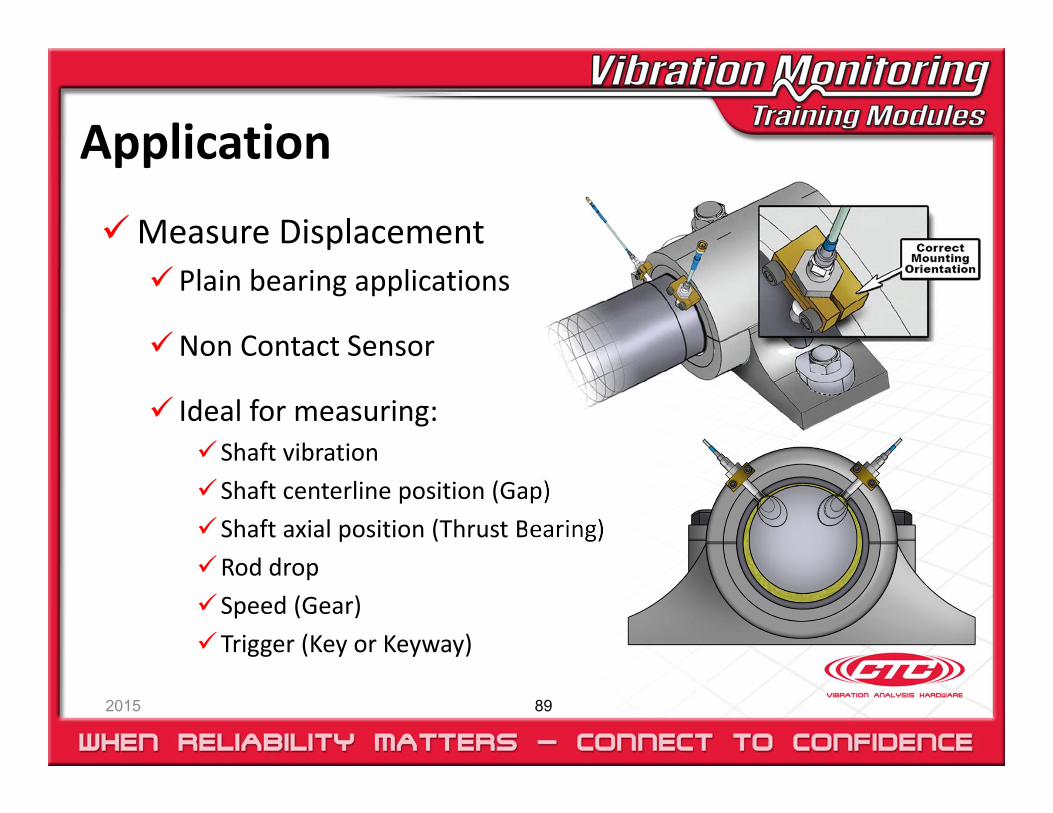
Application
2015 89
Measure Displacement Plain bearing applications
Non Contact Sensor
Ideal for measuring:Shaft vibrationShaft centerline position (Gap)Shaft axial position (Thrust Bearing)Rod dropSpeed (Gear)Trigger (Key or Keyway)
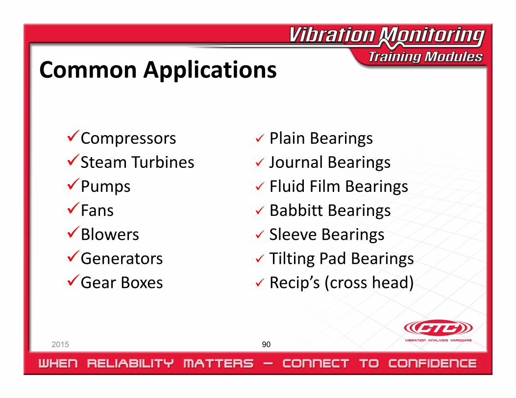
Common Applications
2015 90
CompressorsSteam Turbines PumpsFansBlowersGeneratorsGear Boxes
Plain Bearings Journal Bearings Fluid Film Bearings Babbitt Bearings Sleeve Bearings Tilting Pad Bearings Recip’s (cross head)
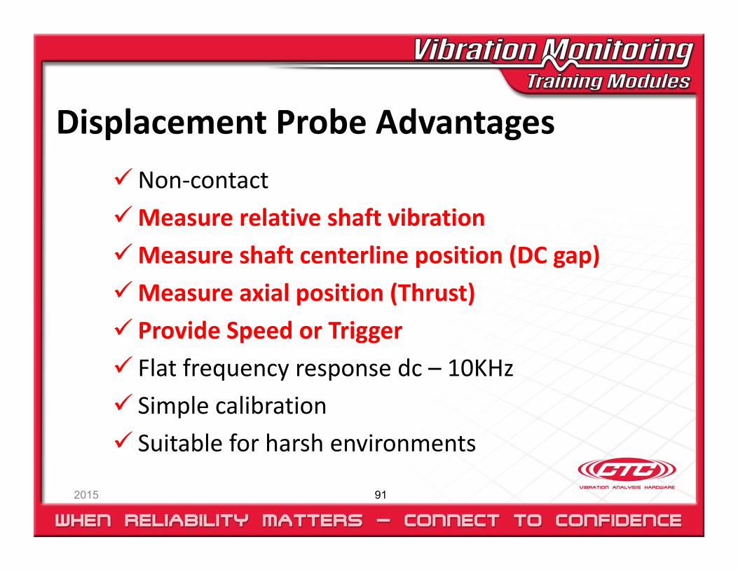
Displacement Probe Advantages
2015 91
Non‐contactMeasure relative shaft vibrationMeasure shaft centerline position (DC gap)Measure axial position (Thrust) Provide Speed or Trigger Flat frequency response dc – 10KHz Simple calibration Suitable for harsh environments
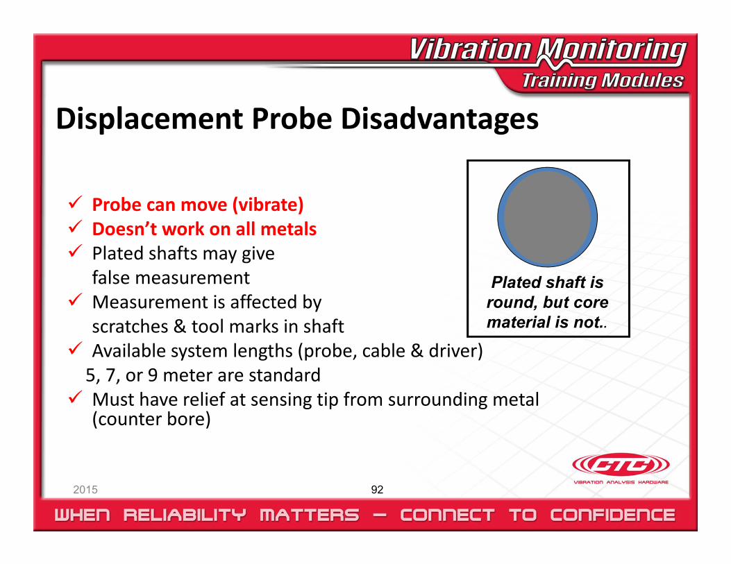
Displacement Probe Disadvantages
2015 92
Probe can move (vibrate) Doesn’t work on all metals Plated shafts may give
false measurement Measurement is affected by
scratches & tool marks in shaft Available system lengths (probe, cable & driver) 5, 7, or 9 meter are standard
Must have relief at sensing tip from surrounding metal (counter bore)
Plated shaft is round, but core material is not..
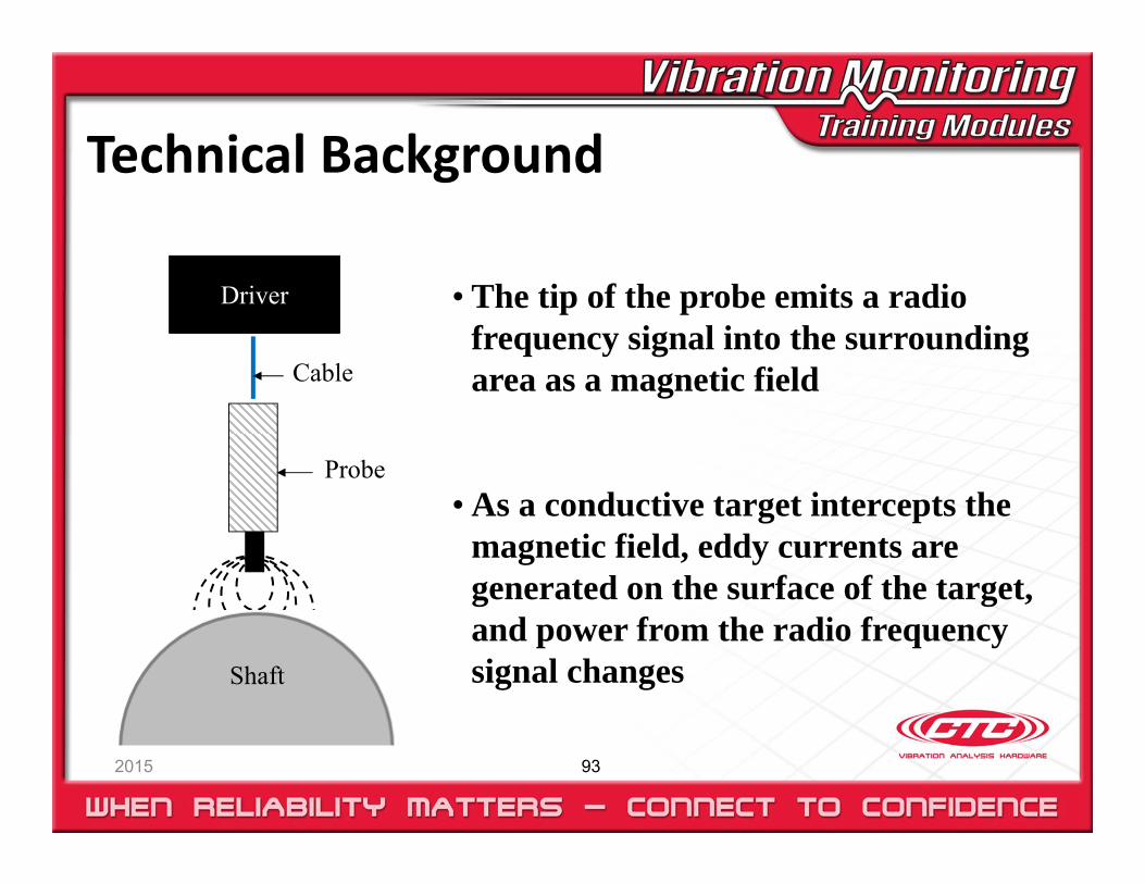
Technical Background
2015 93
• The tip of the probe emits a radio frequency signal into the surrounding area as a magnetic field
• As a conductive target intercepts the magnetic field, eddy currents are generated on the surface of the target, and power from the radio frequency signal changes
Driver
Cable
Probe
Shaft
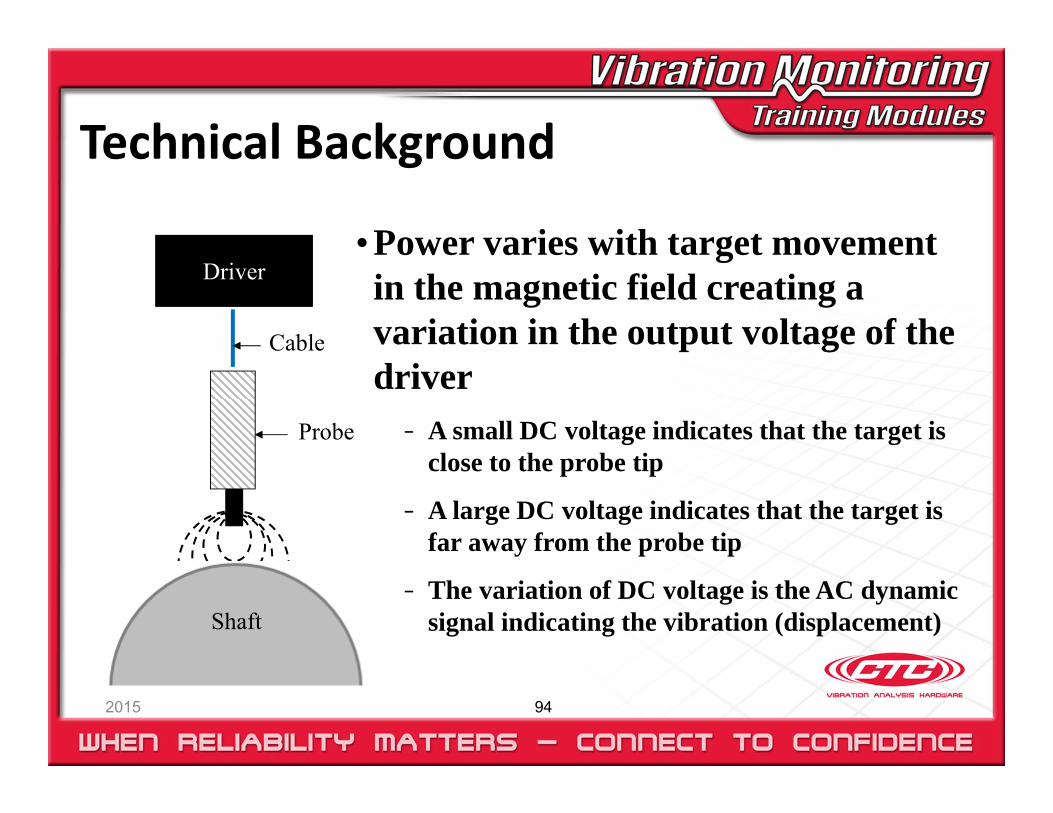
Technical Background
2015 94
• Power varies with target movement in the magnetic field creating a variation in the output voltage of the driver
- A small DC voltage indicates that the target is close to the probe tip
- A large DC voltage indicates that the target is far away from the probe tip
- The variation of DC voltage is the AC dynamic signal indicating the vibration (displacement)
Driver
Cable
Probe
Shaft
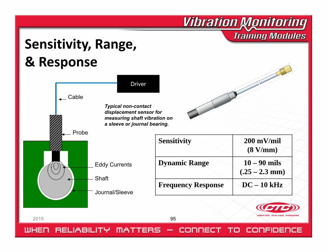
Sensitivity, Range,& Response
2015 95
Sensitivity 200 mV/mil(8 V/mm)
Dynamic Range 10 – 90 mils(.25 – 2.3 mm)
Frequency Response DC – 10 kHz
Driver
Typical non-contact displacement sensor for measuring shaft vibration on a sleeve or journal bearing.
Eddy Currents
Shaft
Journal/Sleeve
Cable
Probe
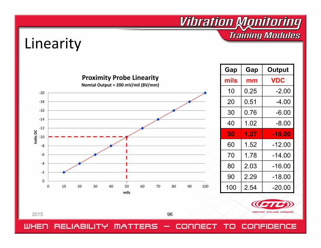
Linearity
2015 96
Gap Gap Outputmils mm VDC10 0.25 -2.0020 0.51 -4.0030 0.76 -6.0040 1.02 -8.0050 1.27 -10.0060 1.52 -12.0070 1.78 -14.0080 2.03 -16.0090 2.29 -18.00100 2.54 -20.00
‐20
‐18
‐16
‐14
‐12
‐10
‐8
‐6
‐4
‐2
00 10 20 30 40 50 60 70 80 90 100
Volts
DC
mils
Proximity Probe LinearityNomial Output = 200 mV/mil (8V/mm)
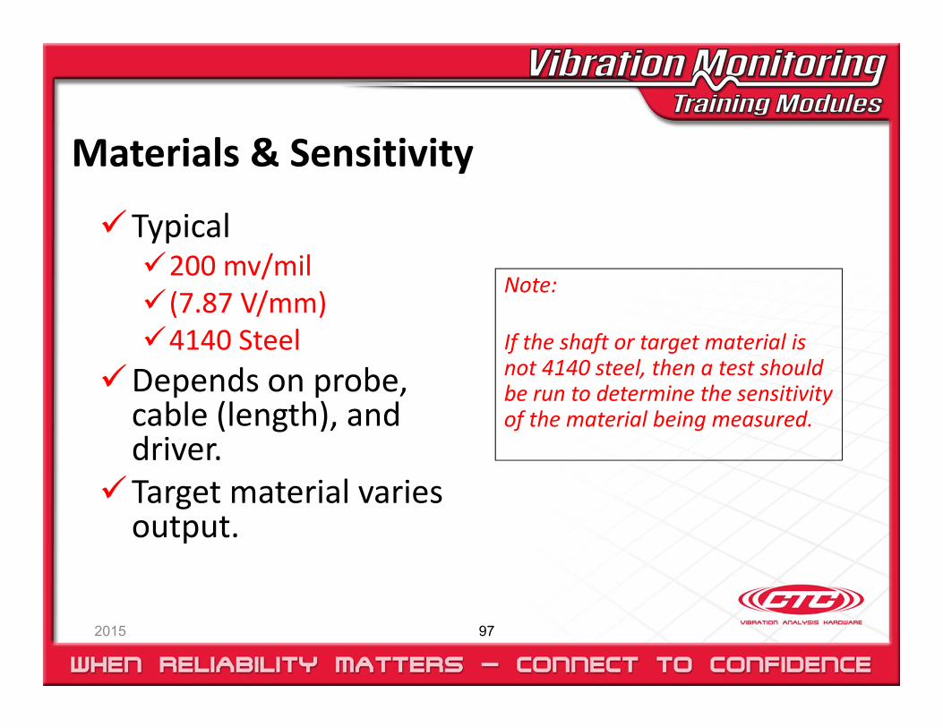
Materials & Sensitivity
2015 97
Typical200 mv/mil (7.87 V/mm)4140 Steel
Depends on probe, cable (length), and driver.
Target material varies output.
Note:
If the shaft or target material is not 4140 steel, then a test should be run to determine the sensitivity of the material being measured.

Durability is Required
2015 98
Proximity probes lead a rough life. Installation, maintenance and overhauls require trained analysts, technicians, or mechanics to properly install and remove the probes. Some probes are actually encapsulated inside the fluid film bearing, and are exposed to the lubrication and heat generated by the bearing. Proper handling and durability are key performance factors.
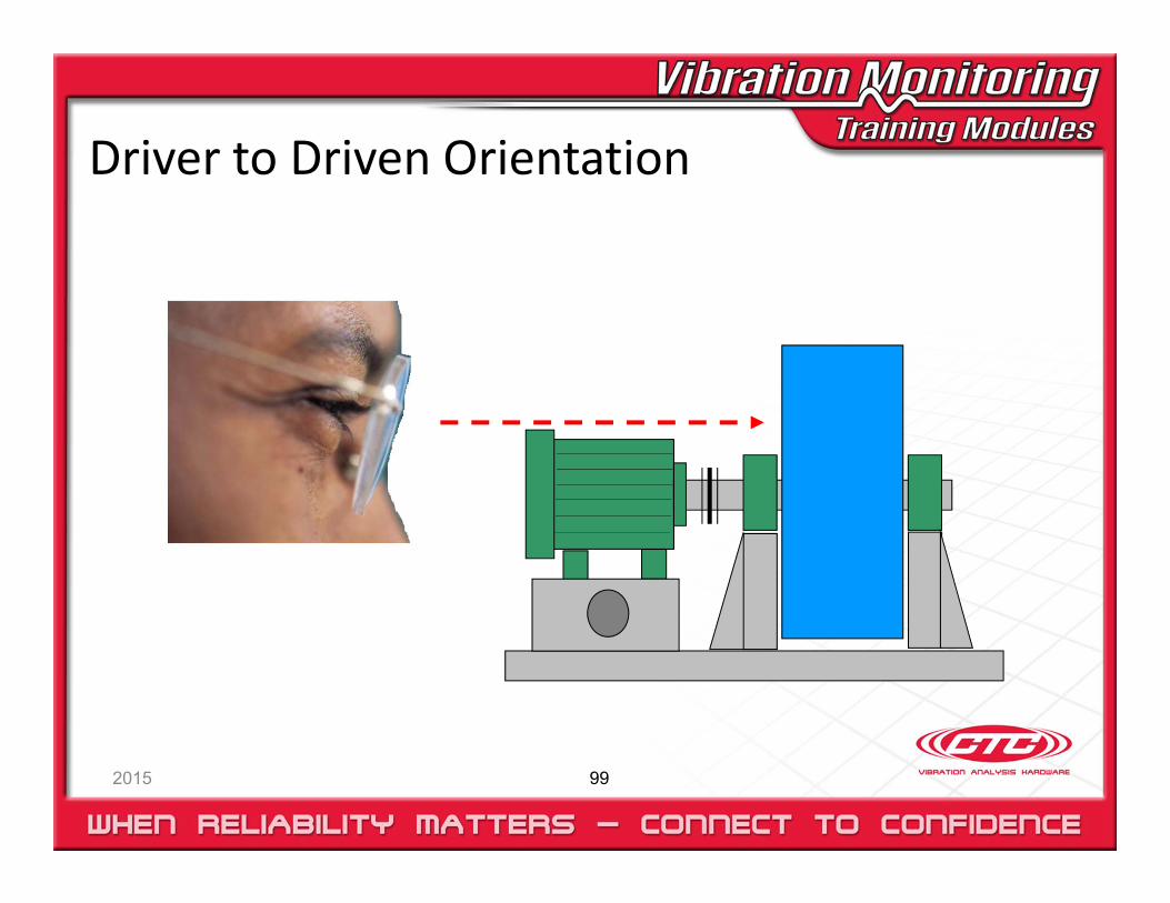
Driver to Driven Orientation
2015 99

API Standard 670
2015 100
• Industry Standard for Proximity Probes
• American Petroleum Institute
• (5th Edition ) 01 November 2014
• www.techstreet.com ≈ $200.00 USD/copy
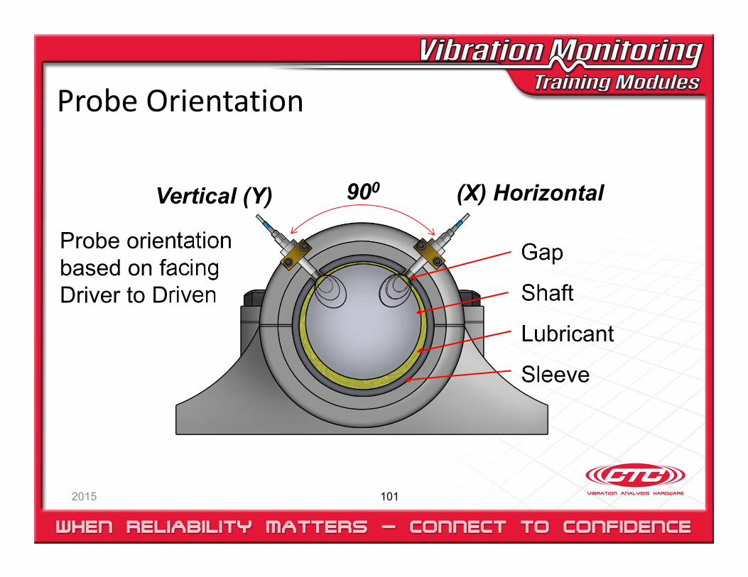
Probe Orientation
2015 101
Probe orientation based on facing Driver to Driven
Gap
Shaft
Lubricant
Sleeve
Vertical (Y) (X) Horizontal900
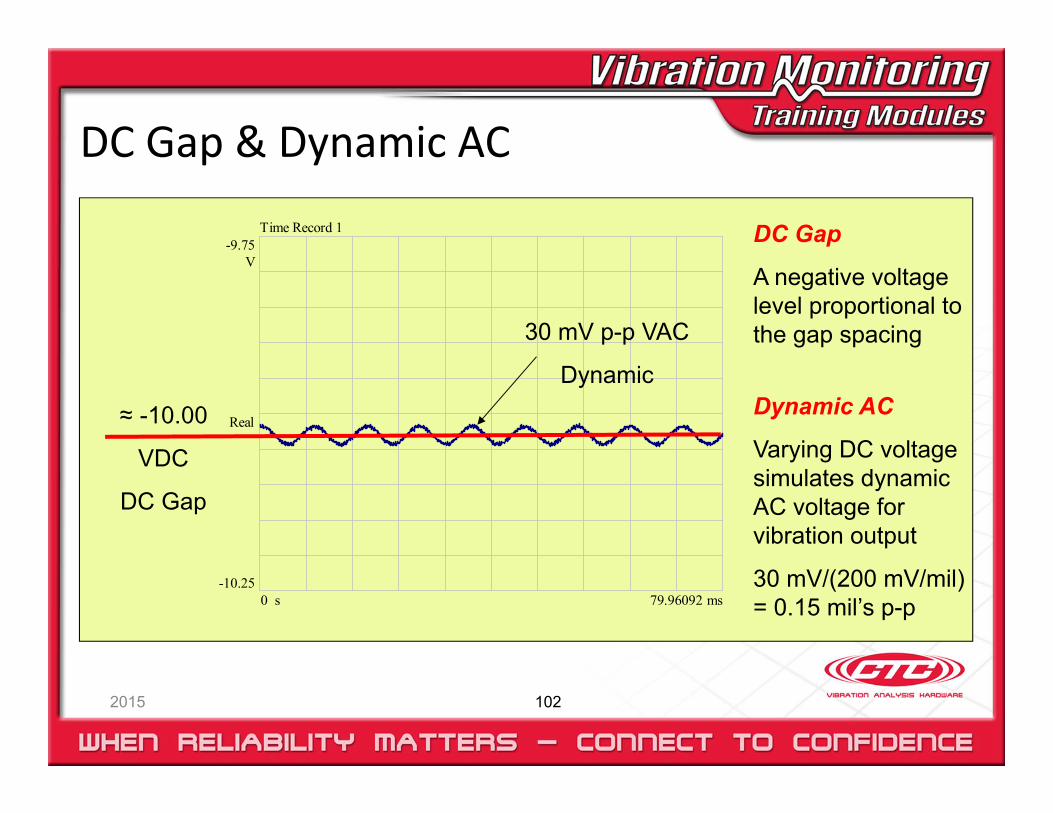
DC Gap & Dynamic AC
2015 102
≈ -10.00
VDC
DC Gap
DC Gap
A negative voltage level proportional to the gap spacing
Dynamic AC
Varying DC voltage simulates dynamic AC voltage for vibration output
30 mV/(200 mV/mil) = 0.15 mil’s p-p
-9.75V
-10.25
Real
ms79.960920 s
Time Record 1
30 mV p-p VAC
Dynamic
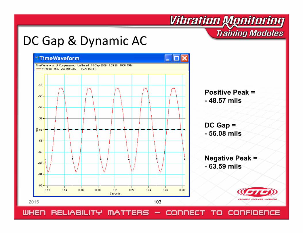
DC Gap & Dynamic AC
Positive Peak = - 48.57 mils
DC Gap = - 56.08 mils
Negative Peak = - 63.59 mils
2015 103
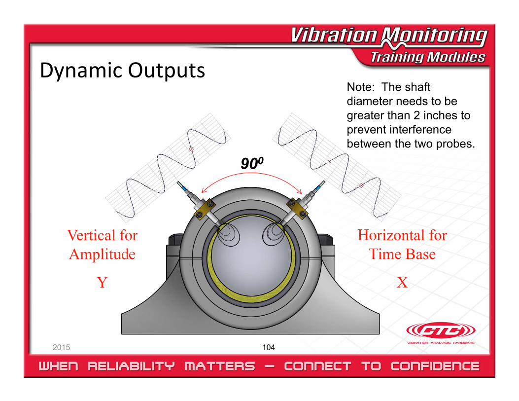
Dynamic Outputs
2015 104
Vertical for Amplitude
Y
Horizontal for Time Base
X
900
Note: The shaft diameter needs to be greater than 2 inches to prevent interference between the two probes.
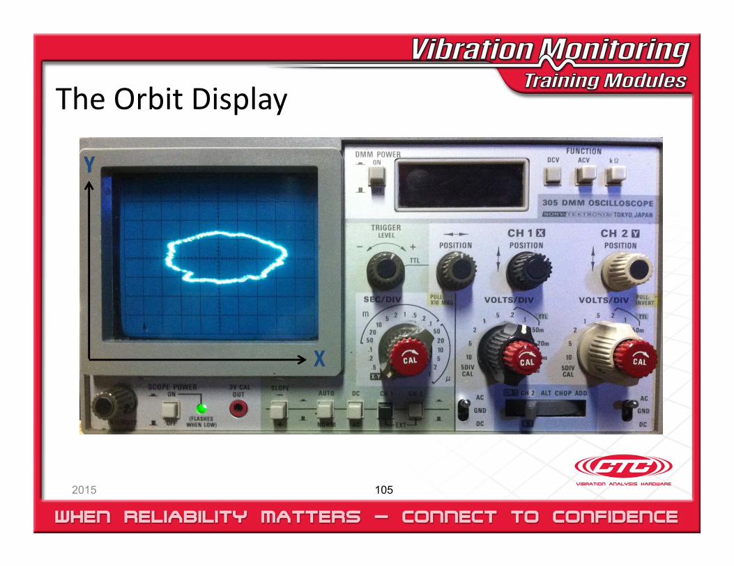
The Orbit Display
2015 105
Y
X
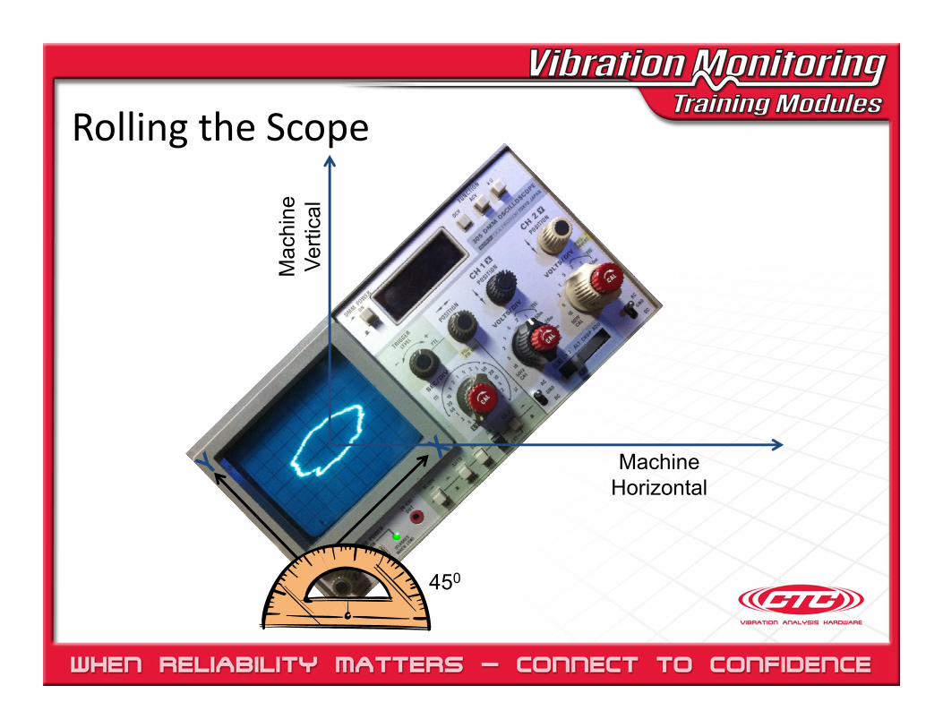
Rolling the Scope
450
Machine Horizontal
Mac
hine
Ve
rtica
l
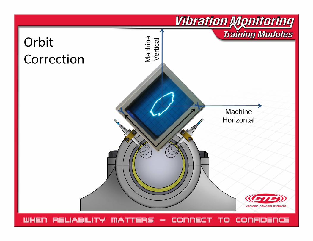
Orbit Correction
Machine Horizontal
Mac
hine
Ve
rtica
l
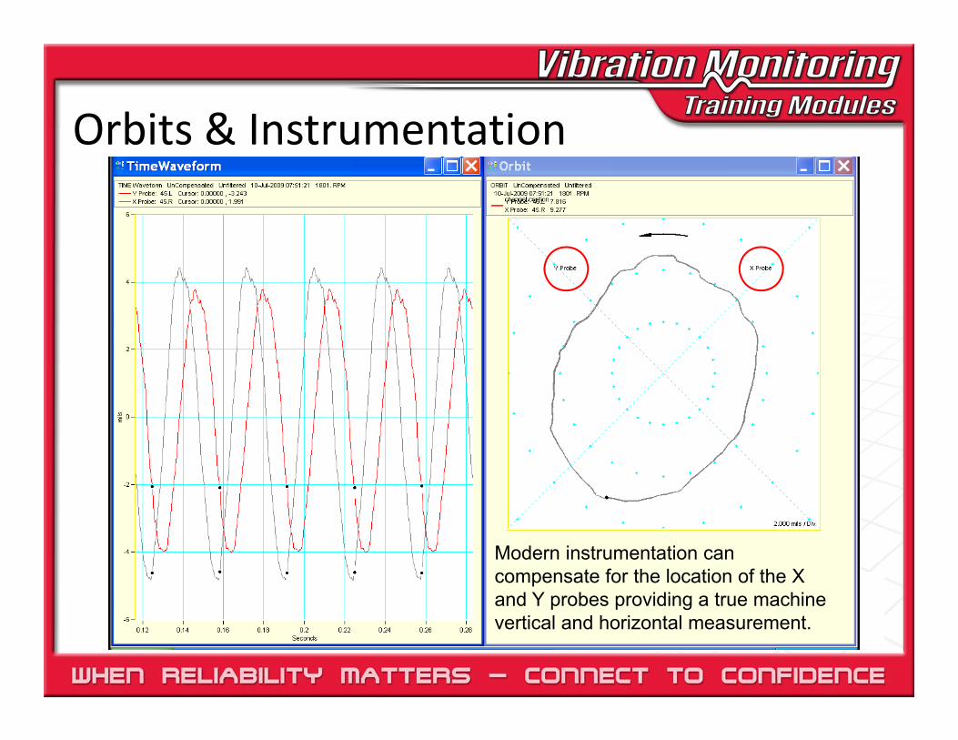
Orbits & Instrumentation
Modern instrumentation can compensate for the location of the X and Y probes providing a true machine vertical and horizontal measurement.
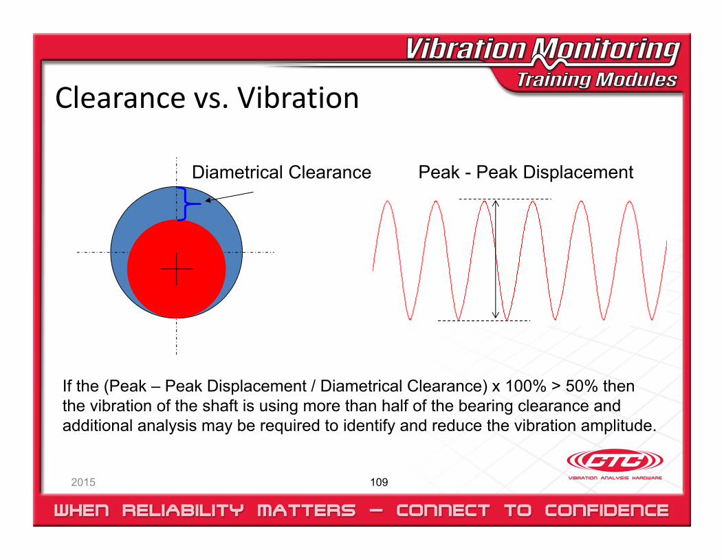
Clearance vs. Vibration
2015 109
Diametrical Clearance Peak - Peak Displacement
If the (Peak – Peak Displacement / Diametrical Clearance) x 100% > 50% then the vibration of the shaft is using more than half of the bearing clearance and additional analysis may be required to identify and reduce the vibration amplitude.
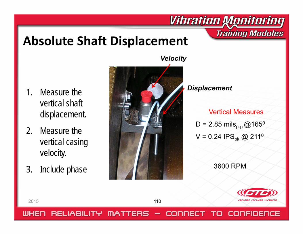
Absolute Shaft Displacement
2015 110
Displacement
Velocity
1. Measure the vertical shaft displacement.
2. Measure the vertical casing velocity.
3. Include phase
Vertical Measures
D = 2.85 milsp-p @1650
V = 0.24 IPSpk @ 2110
3600 RPM
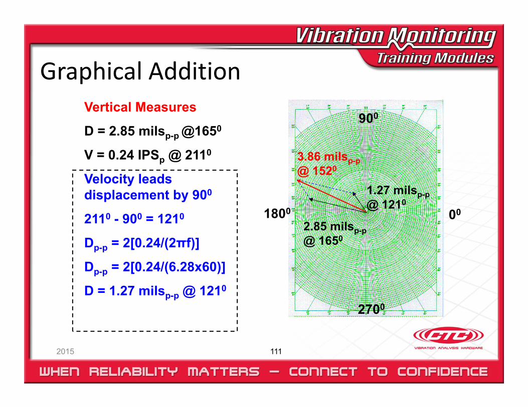
Graphical Addition
2015 111
Vertical Measures
D = 2.85 milsp-p @1650
V = 0.24 IPSp @ 2110
Velocity leads displacement by 900
2110 - 900 = 1210
Dp-p = 2[0.24/(2πf)]
Dp-p = 2[0.24/(6.28x60)]
D = 1.27 milsp-p @ 1210
900
001800
2700
1.27 milsp-p@ 1210
2.85 milsp-p@ 1650
3.86 milsp-p@ 1520
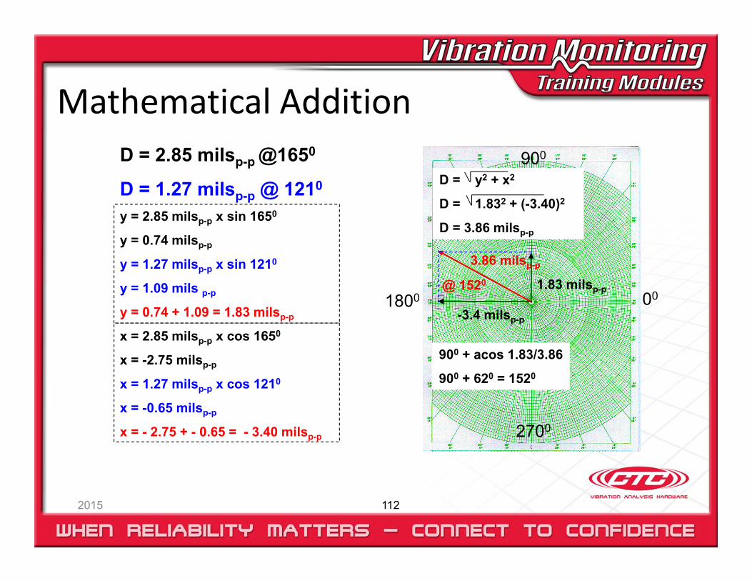
Mathematical Addition
2015 112
D = 2.85 milsp-p @1650
D = 1.27 milsp-p @ 1210
y = 2.85 milsp-p x sin 1650
y = 0.74 milsp-p
y = 1.27 milsp-p x sin 1210
y = 1.09 mils p-p
y = 0.74 + 1.09 = 1.83 milsp-p
x = 2.85 milsp-p x cos 1650
x = -2.75 milsp-p
x = 1.27 milsp-p x cos 1210
x = -0.65 milsp-p
x = - 2.75 + - 0.65 = - 3.40 milsp-p
900
0018001.83 milsp-p
-3.4 milsp-p
3.86 milsp-p
@ 1520
D = y2 + x2
D = 1.832 + (-3.40)2
D = 3.86 milsp-p
900 + acos 1.83/3.86
900 + 620 = 1520
2700
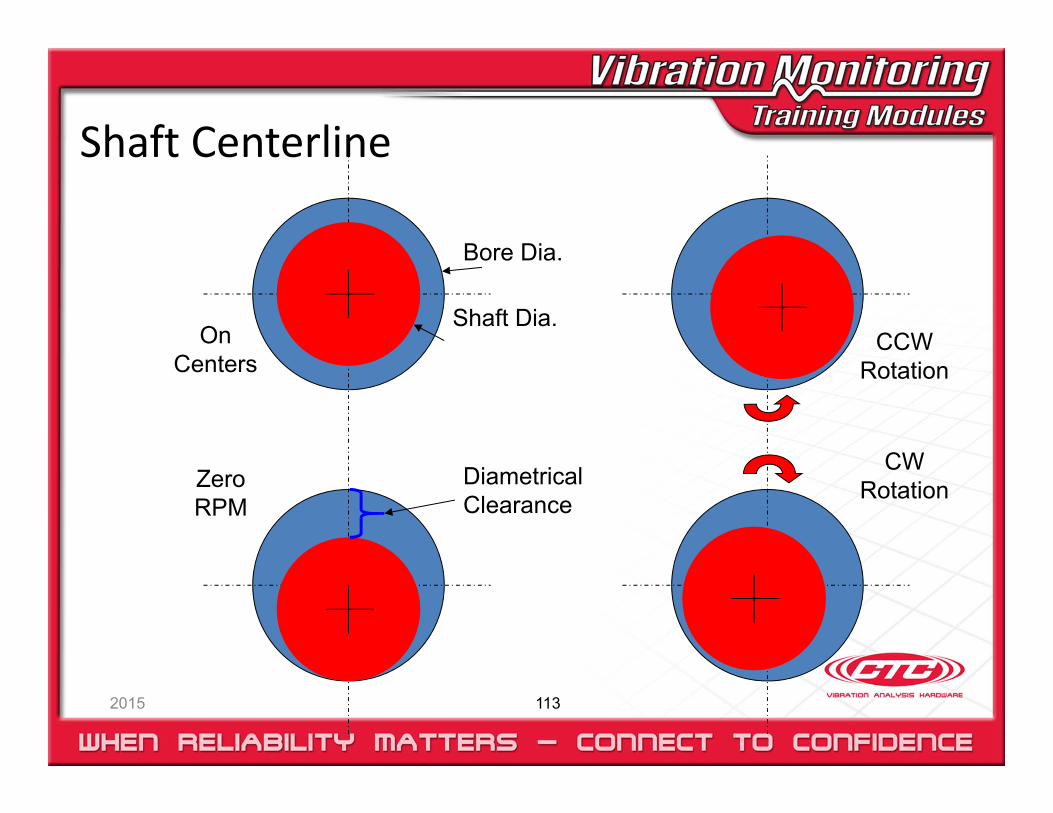
Shaft Centerline
2015 113
On Centers
Bore Dia.
Shaft Dia.
Zero RPM
CCW Rotation
CW RotationDiametrical
Clearance
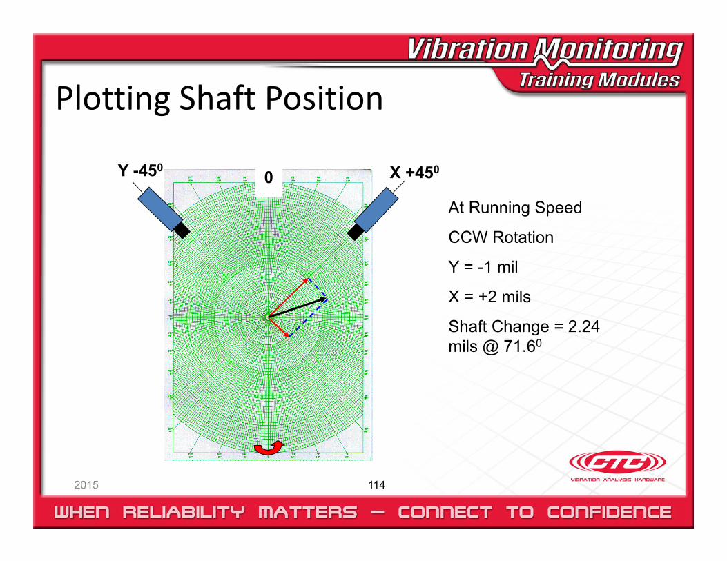
Plotting Shaft Position
2015 114
At Running Speed
CCW Rotation
Y = -1 mil
X = +2 mils
Shaft Change = 2.24 mils @ 71.60
0 Y -450 X +450
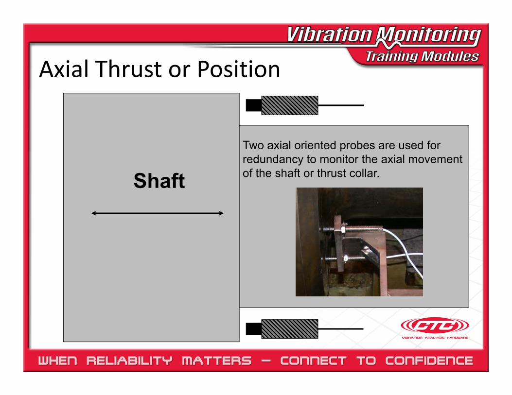
Axial Thrust or Position
Shaft
Two axial oriented probes are used for redundancy to monitor the axial movement of the shaft or thrust collar.
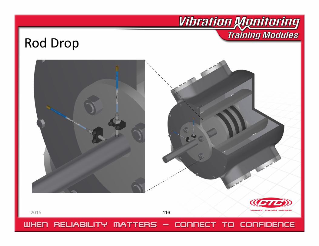
Rod Drop
2015 116
2015 117
Natural Frequency
2015 118
A result of the Mass (m) and Stiffness (k) of the machine design
Resonance occurs when a natural frequency is excited by a force
Critical speed occurs when the machine speed matches the natural frequency and creates resonance
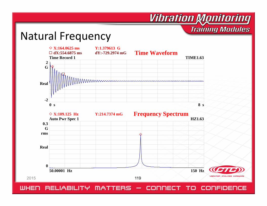
Natural Frequency
2015 119
0.3G
rms
0
Real
Hz150 50.00001 Hz
Auto Pwr Spec 1 HZ1.63
2G
-2
Real
s8 0 s
Time Record 1 TIME1.63
X:109.125 Hz Y:214.7374 mG
dX:554.6875 ms dY:-729.2974 mGX:164.0625 ms Y:1.379613 G
Time Waveform
Frequency Spectrum
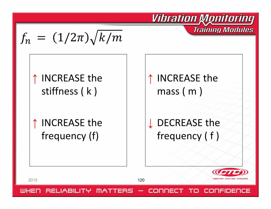
2015 120
↑ INCREASE the stiffness ( k )
↑ INCREASE the frequency (f)
↑ INCREASE the mass ( m )
↓ DECREASE the frequency ( f )
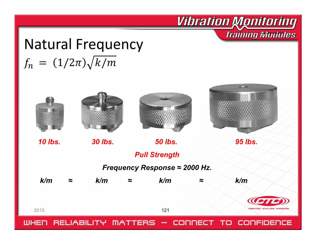
Natural Frequency
2015 121
10 lbs. 30 lbs. 50 lbs. 95 lbs.
Pull Strength
Frequency Response ≈ 2000 Hz.
k/m ≈ k/m ≈ k/m ≈ k/m
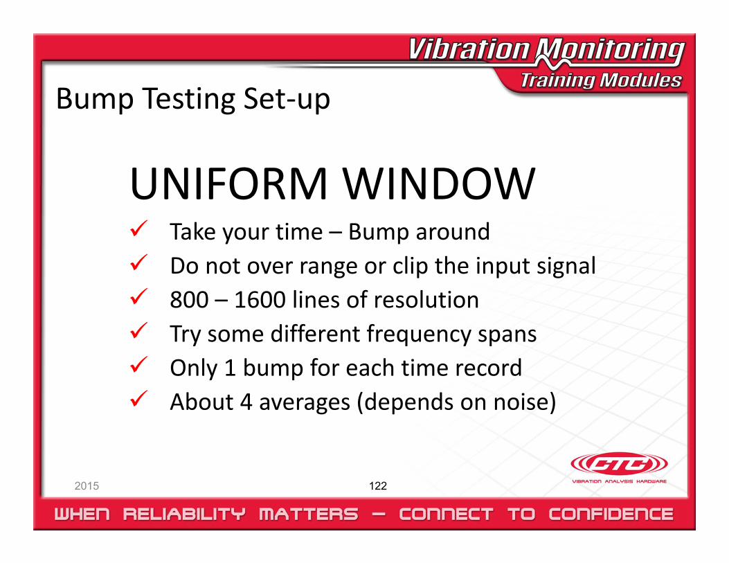
Bump Testing Set‐up
2015 122
UNIFORM WINDOW Take your time – Bump around Do not over range or clip the input signal 800 – 1600 lines of resolution Try some different frequency spans Only 1 bump for each time record About 4 averages (depends on noise)

Uniform Window
2015 123
The Uniform window should be used for bump testing.
If you use the Hanning or Flat Top windows, they will filter out the response from the impact
Uniform
Hanning
Flat Top
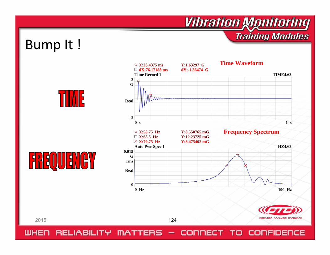
Bump It !
2015 124
2G
-2
Real
s1 0 s
Time Record 1 TIME4.63
0.015G
rms
0
Real
Hz100 0 Hz
Auto Pwr Spec 1 HZ4.63
dX:76.17188 ms dY:-1.36474 GX:23.4375 ms Y:1.63297 G
X:70.75 Hz Y:8.475402 mGX:65.5 Hz Y:12.23725 mGX:58.75 Hz Y:8.550765 mG
Time Waveform
Frequency Spectrum
Mental Health Check !
2015 125
2G
-2
Real
s1 0 s
Time Record 1 TIME4.63
0.015G
rms
0
Real
Hz100 0 Hz
Auto Pwr Spec 1 HZ4.63
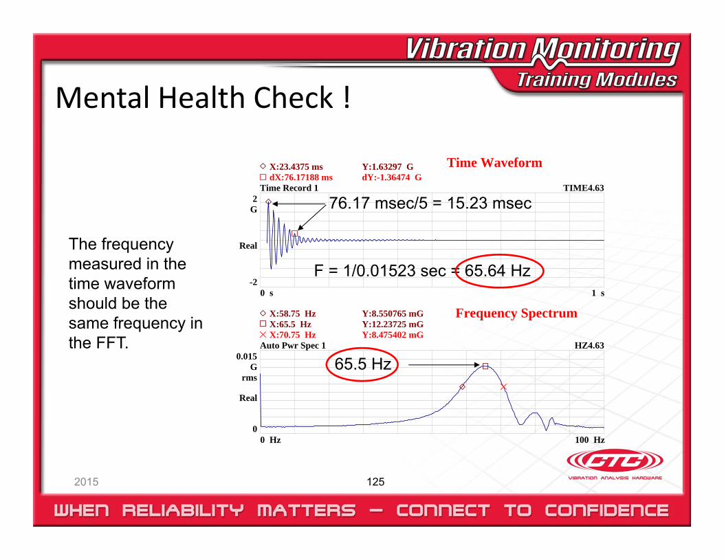
dX:76.17188 ms dY:-1.36474 GX:23.4375 ms Y:1.63297 G
X:70.75 Hz Y:8.475402 mGX:65.5 Hz Y:12.23725 mGX:58.75 Hz Y:8.550765 mG
Time Waveform
Frequency Spectrum
76.17 msec/5 = 15.23 msec
F = 1/0.01523 sec = 65.64 Hz
65.5 Hz
The frequency measured in the time waveform should be the same frequency in the FFT.
Time Waveform
2015 126
2G
-2
Real
s1 0 s
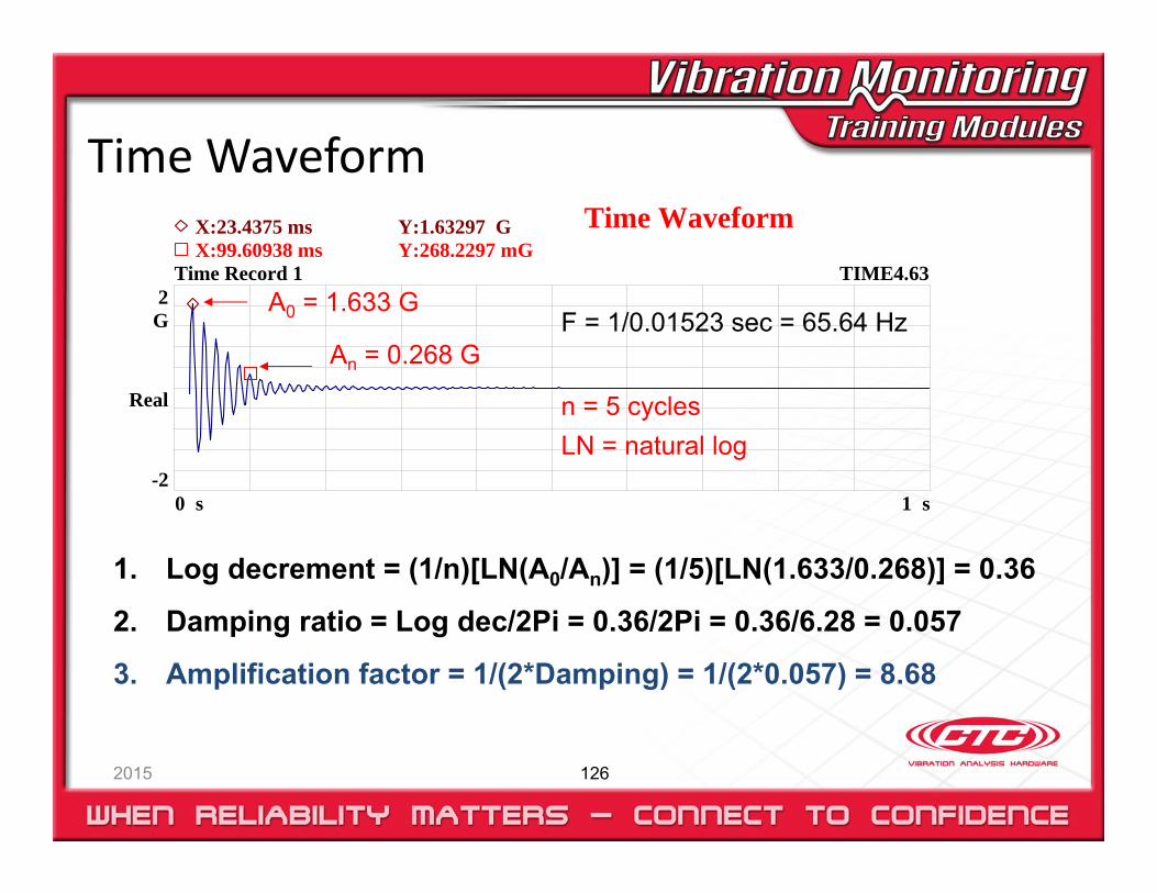
Time Record 1 TIME4.63X:99.60938 ms Y:268.2297 mGX:23.4375 ms Y:1.63297 G Time Waveform
1. Log decrement = (1/n)[LN(A0/An)] = (1/5)[LN(1.633/0.268)] = 0.36
2. Damping ratio = Log dec/2Pi = 0.36/2Pi = 0.36/6.28 = 0.057
3. Amplification factor = 1/(2*Damping) = 1/(2*0.057) = 8.68
A0 = 1.633 G
An = 0.268 G
n = 5 cyclesLN = natural log
F = 1/0.01523 sec = 65.64 Hz
FFT or Spectrum
2015 127
0.015G
rms
0
Real
Hz100 0 Hz
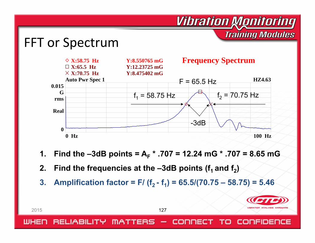
Auto Pwr Spec 1 HZ4.63X:70.75 Hz Y:8.475402 mGX:65.5 Hz Y:12.23725 mGX:58.75 Hz Y:8.550765 mG Frequency Spectrum
F = 65.5 Hz
f2 = 70.75 Hzf1 = 58.75 Hz
-3dB
1. Find the –3dB points = AF * .707 = 12.24 mG * .707 = 8.65 mG
2. Find the frequencies at the –3dB points (f1 and f2)
3. Amplification factor = F/ (f2 - f1) = 65.5/(70.75 – 58.75) = 5.46
Bump Testing Summary
2015 128
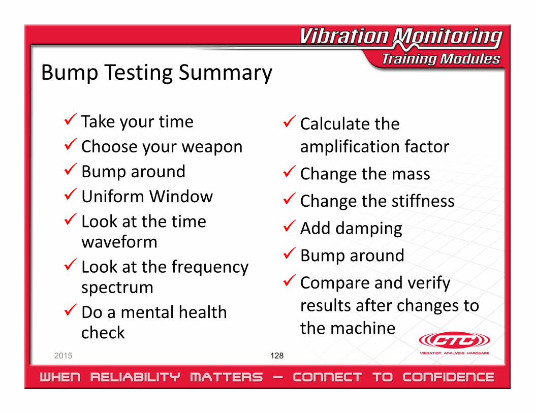
Take your time Choose your weapon Bump aroundUniform Window Look at the time waveform
Look at the frequency spectrum
Do a mental health check
Calculate the amplification factor
Change the mass Change the stiffness Add damping Bump around Compare and verify results after changes to the machine
1x (Running Speed)
2015 129
Mass Unbalance 1x• Critical Speed 1x• Misalignment 1x, 2x, 3x• Looseness 1x, 2x, 3x, 4x, 5x, ….• Runout 1x
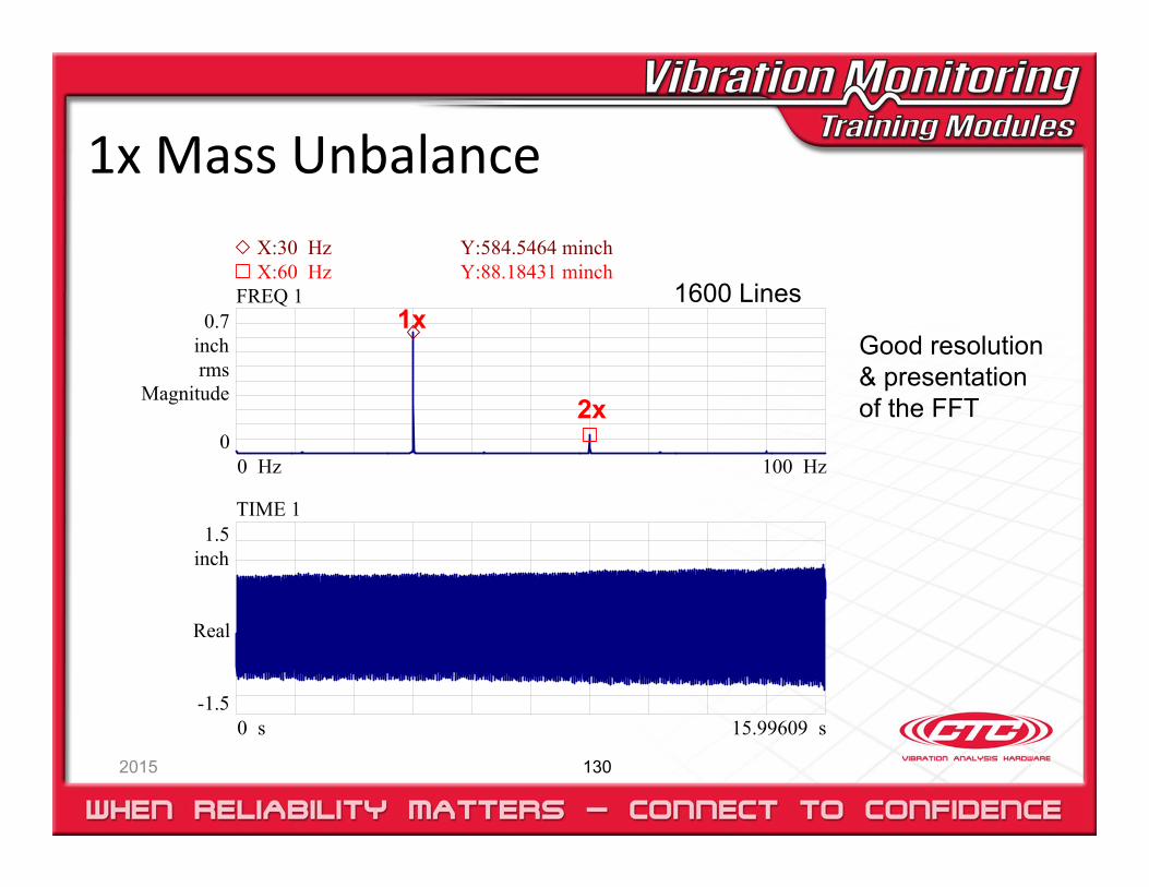
1x Mass Unbalance
2015 130
1.5inch
-1.5
Real
s15.99609 0 s
TIME 1
0.7inchrms
0
Magnitude
Hz100 0 Hz
FREQ 1X:60 Hz Y:88.18431 minchX:30 Hz Y:584.5464 minch
1x
2x
1600 Lines
Good resolution & presentation of the FFT
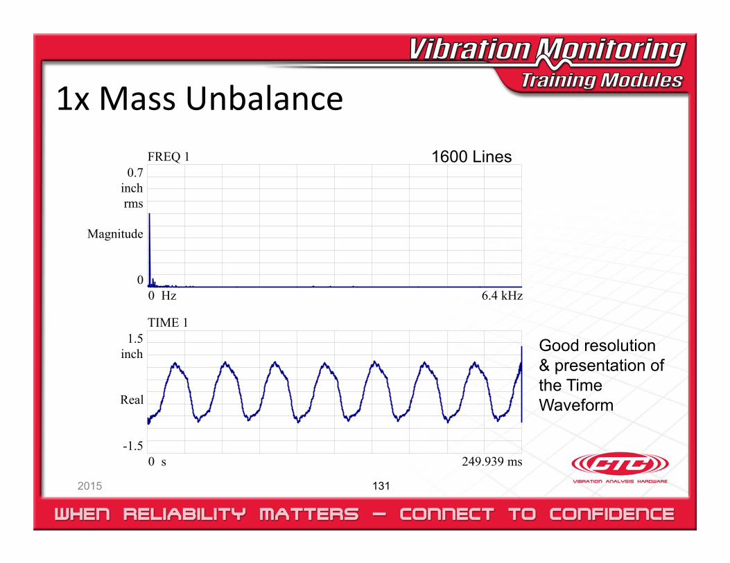
1x Mass Unbalance
2015 131
1.5inch
-1.5
Real
ms249.9390 s
TIME 1
0.7inchrms
0
Magnitude
kHz6.40 Hz
FREQ 1 1600 Lines
Good resolution & presentation of the Time Waveform
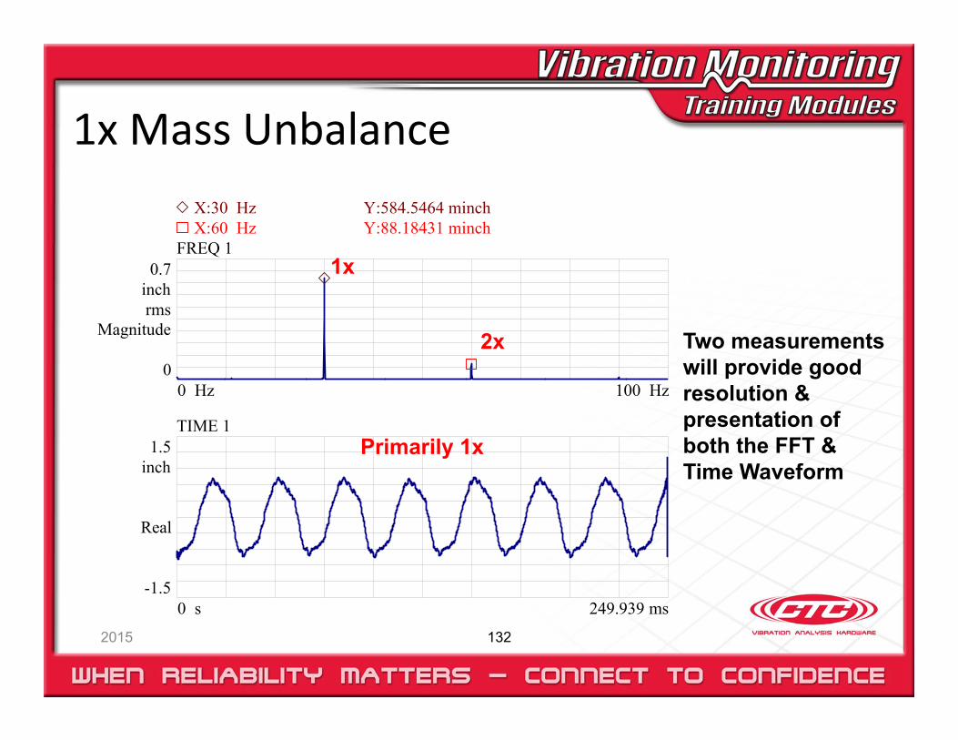
1x Mass Unbalance
2015 132
Two measurements will provide good resolution & presentation of both the FFT & Time Waveform
1.5inch
-1.5
Real
ms249.9390 s
TIME 1
0.7inchrms
0
Magnitude
Hz100 0 Hz
FREQ 1X:60 Hz Y:88.18431 minchX:30 Hz Y:584.5464 minch
1x
2x
Primarily 1x
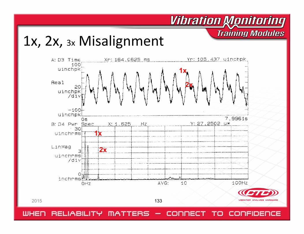
1x, 2x, 3x Misalignment
2015 133
1x
2x
1x
2x
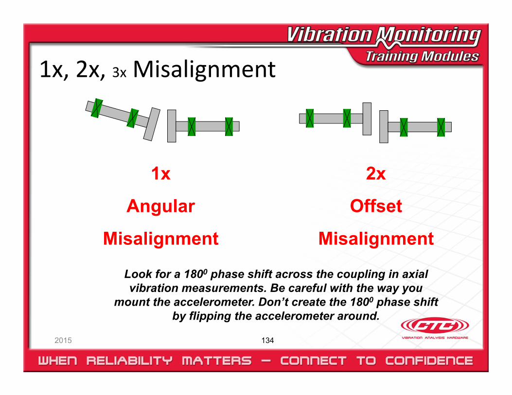
1x, 2x, 3x Misalignment
2015 134
1x
Angular
Misalignment
2x
Offset
Misalignment
Look for a 1800 phase shift across the coupling in axial vibration measurements. Be careful with the way you
mount the accelerometer. Don’t create the 1800 phase shift by flipping the accelerometer around.
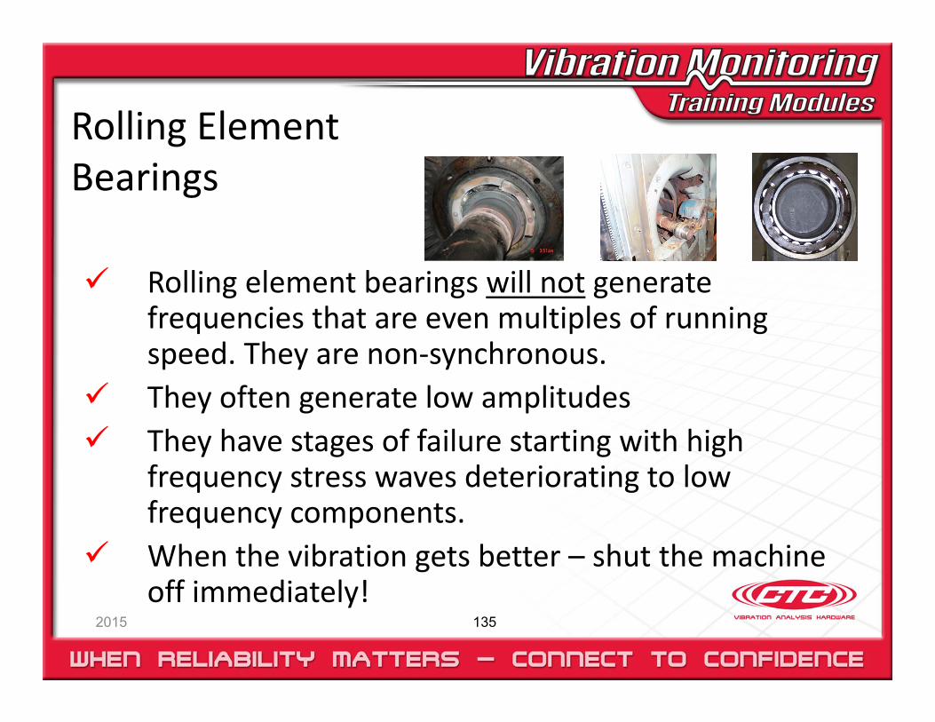
Rolling Element Bearings
2015 135
Rolling element bearings will not generate frequencies that are even multiples of running speed. They are non‐synchronous.
They often generate low amplitudes They have stages of failure starting with high
frequency stress waves deteriorating to low frequency components.
When the vibration gets better – shut the machine off immediately!
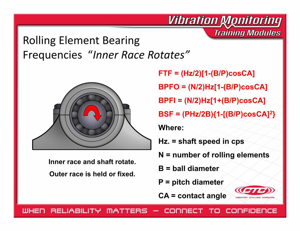
Rolling Element Bearing Frequencies “Inner Race Rotates”
Inner race and shaft rotate.
Outer race is held or fixed.
FTF = (Hz/2)[1-(B/P)cosCA]
BPFO = (N/2)Hz[1-(B/P)cosCA]
BPFI = (N/2)Hz[1+(B/P)cosCA]
BSF = (PHz/2B){1-[(B/P)cosCA]2}
Where:
Hz. = shaft speed in cps
N = number of rolling elements
B = ball diameter
P = pitch diameter
CA = contact angle
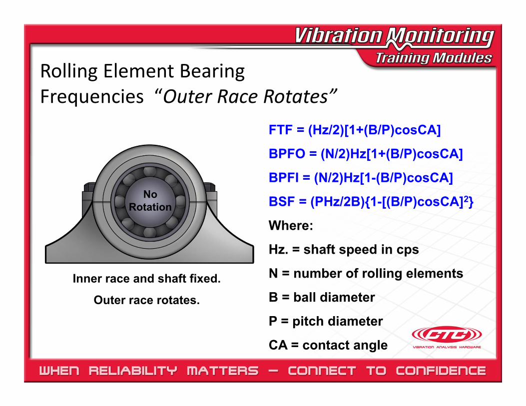
Rolling Element Bearing Frequencies “Outer Race Rotates”
Inner race and shaft fixed.
Outer race rotates.
FTF = (Hz/2)[1+(B/P)cosCA]
BPFO = (N/2)Hz[1+(B/P)cosCA]
BPFI = (N/2)Hz[1-(B/P)cosCA]
BSF = (PHz/2B){1-[(B/P)cosCA]2}
Where:
Hz. = shaft speed in cps
N = number of rolling elements
B = ball diameter
P = pitch diameter
CA = contact angle
No Rotation
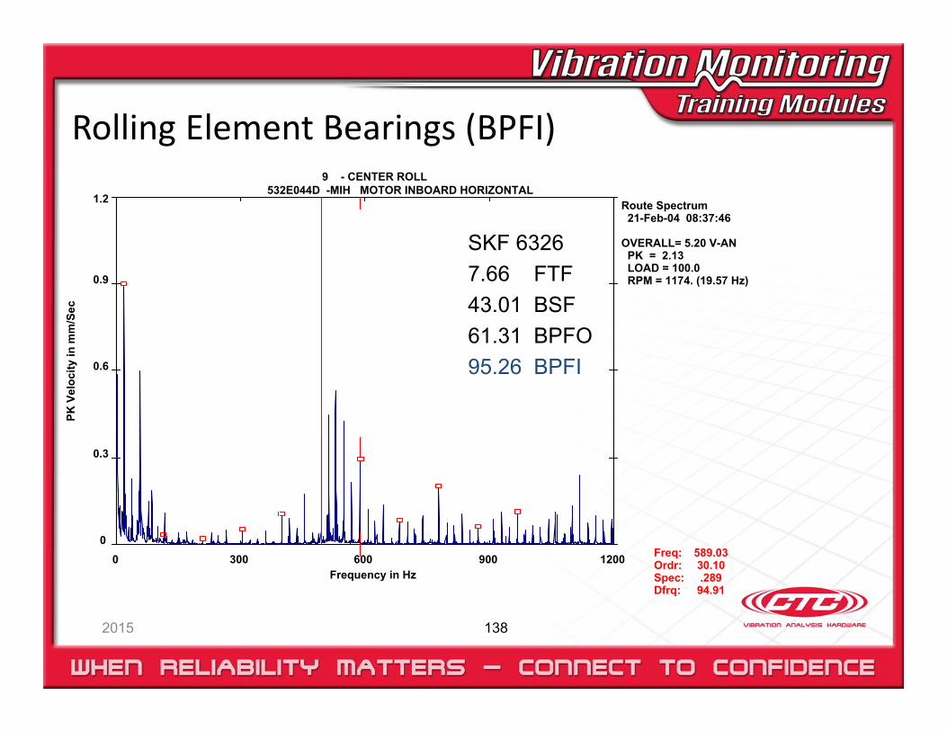
Rolling Element Bearings (BPFI)
2015 138
9 - CENTER ROLL532E044D -MIH MOTOR INBOARD HORIZONTAL
Route Spectrum 21-Feb-04 08:37:46
OVERALL= 5.20 V-AN PK = 2.13 LOAD = 100.0 RPM = 1174. (19.57 Hz)
0 300 600 900 12000
0.3
0.6
0.9
1.2
Frequency in Hz
PK V
eloc
ity in
mm
/Sec
Freq: Ordr: Spec: Dfrq:
589.03 30.10 .289 94.91
SKF 63267.66 FTF43.01 BSF61.31 BPFO95.26 BPFI
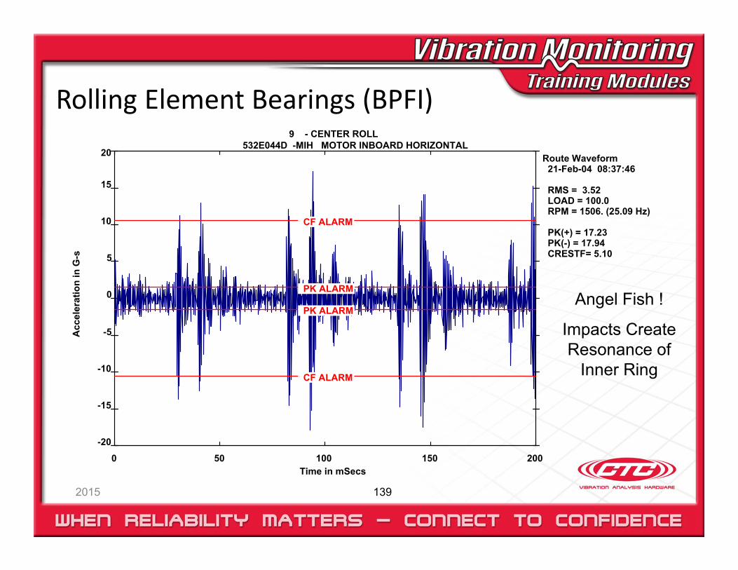
Rolling Element Bearings (BPFI)
2015 139
9 - CENTER ROLL532E044D -MIH MOTOR INBOARD HORIZONTAL
Route Waveform 21-Feb-04 08:37:46
RMS = 3.52 LOAD = 100.0 RPM = 1506. (25.09 Hz)
PK(+) = 17.23 PK(-) = 17.94 CRESTF= 5.10
0 50 100 150 200-20
-15
-10
-5
0
5
10
15
20
Time in mSecs
Acc
eler
atio
n in
G-s
CF ALARM
CF ALARM
PK ALARM
PK ALARM Angel Fish !
Impacts Create Resonance of
Inner Ring
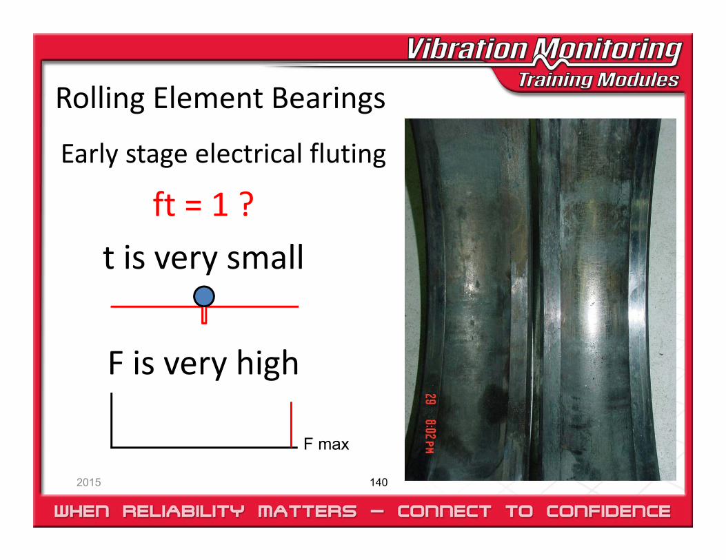
Rolling Element Bearings
2015 140
ft = 1 ?t is very small
F is very high
F max
Early stage electrical fluting
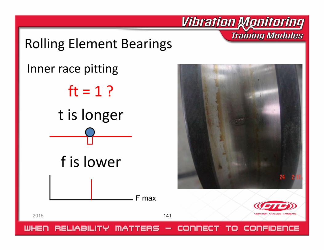
Rolling Element Bearings
2015 141
ft = 1 ?t is longer
f is lower
F max
Inner race pitting
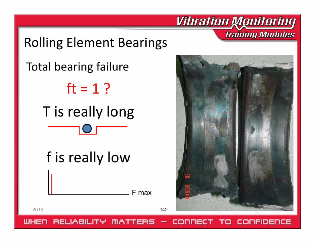
Rolling Element Bearings
2015 142
ft = 1 ?T is really long
f is really low
F max
Total bearing failure

Rolling Element Bearings
As the frequency gets lower bad things are happening !
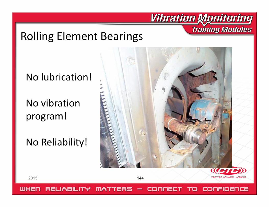
Rolling Element Bearings
2015 144
No lubrication!
No vibration program!
No Reliability!

Rolling Element Bearings ?
You need all of the rolling elements, in the same orientation, a good cage, and a solid inner race to have a quality bearing and good vibration measurement!

Rolling Element Bearings
2015 146
Severe Electrical Fluting
Gear Mesh
2015 147
Number of Teeth x Speed of the Shaft it is mounted on.
Sidebands around gear mesh will be spaced at the shaft speed the gear is mounted on.
Typically the vibration will be in the axial direction
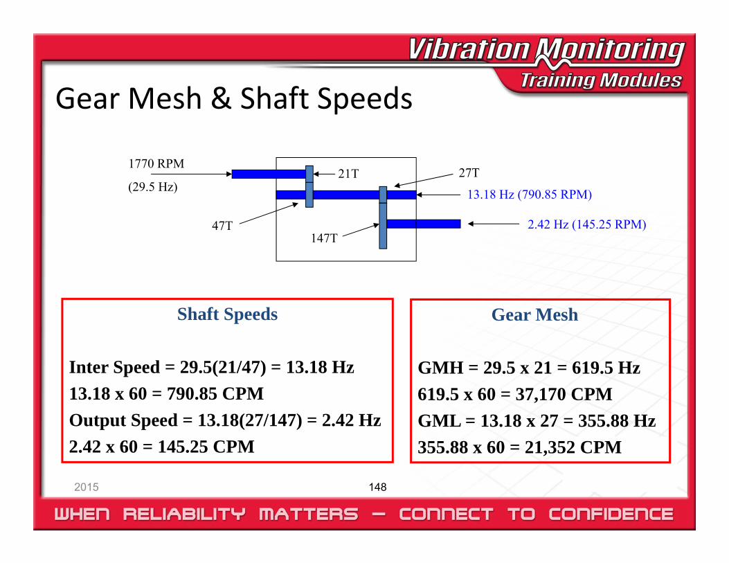
Gear Mesh & Shaft Speeds
2015 148
1770 RPM
(29.5 Hz)21T
47T
27T
147T
13.18 Hz (790.85 RPM)
2.42 Hz (145.25 RPM)
Shaft Speeds
Inter Speed = 29.5(21/47) = 13.18 Hz13.18 x 60 = 790.85 CPMOutput Speed = 13.18(27/147) = 2.42 Hz2.42 x 60 = 145.25 CPM
Gear Mesh
GMH = 29.5 x 21 = 619.5 Hz619.5 x 60 = 37,170 CPMGML = 13.18 x 27 = 355.88 Hz355.88 x 60 = 21,352 CPM
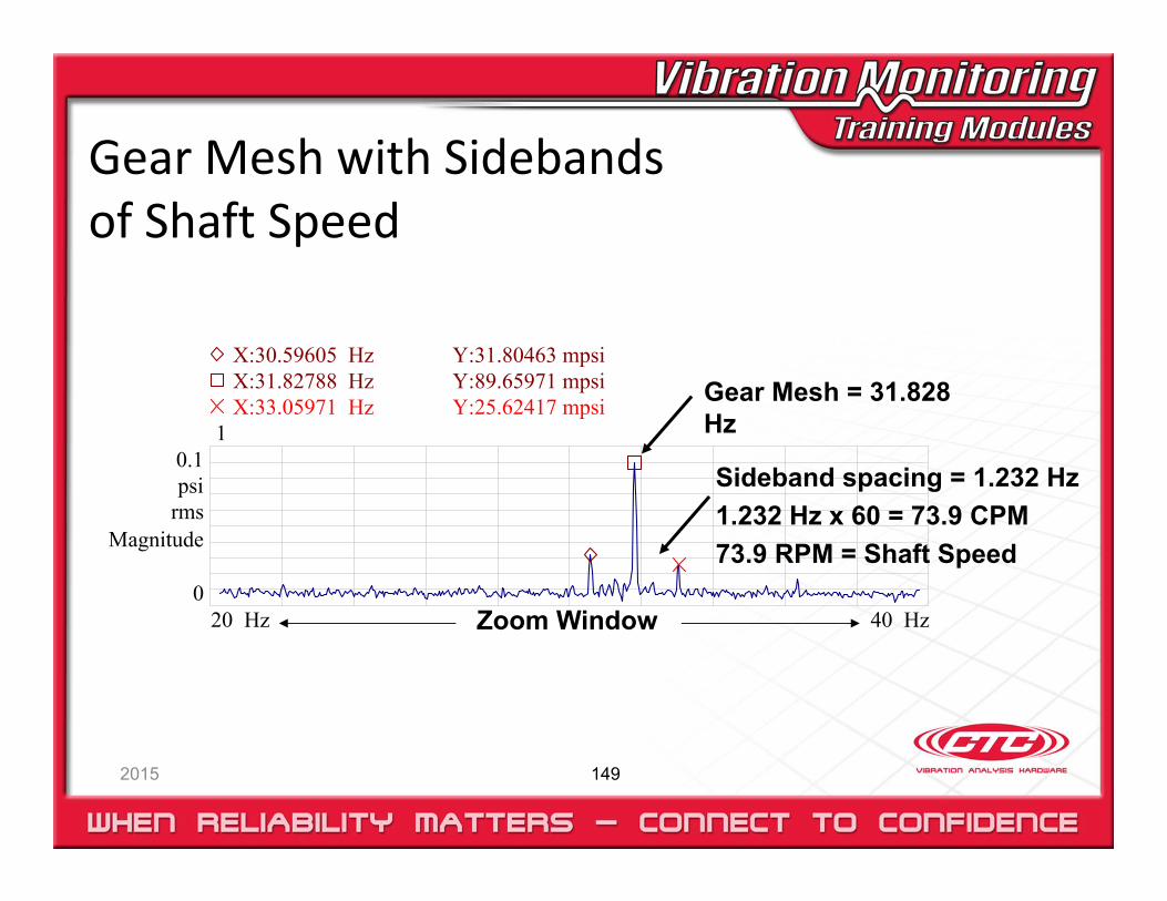
Gear Mesh with Sidebandsof Shaft Speed
2015 149
0.1psi
rms
0
Magnitude
Hz40 20 Hz
1X:33.05971 Hz Y:25.62417 mpsiX:31.82788 Hz Y:89.65971 mpsiX:30.59605 Hz Y:31.80463 mpsi
Gear Mesh = 31.828 Hz
Sideband spacing = 1.232 Hz1.232 Hz x 60 = 73.9 CPM73.9 RPM = Shaft Speed
Zoom Window
Fans
2015 150
Blade Pass• Number of Blades x Speed of the Shaft the
rotor is mounted on.• Look at the damper and duct work for flow
and restrictions.• Blade clearance, discharge angle, wear & tear
Unbalance, misalignment, bearings
Pumps
2015 151
Vane Pass• Number of Vanes x Speed of the Shaft the rotor is mounted on.• Look at the input and output pressures• Vane clearance, discharge angle, wear & tear
Recirculation• Random noise in FFT & Time Waveform• Axial shuttling, High back pressure, Low flow rate• Fluid being forced back into pump
Cavitation• Random noise in the FFT & Time Waveform• Audible noise, Low back pressure, High flow rate• Air entrained in fluid
Unbalance, misalignment, bearings
Motors
2015 152
Synchronous Speed• (2 x Line Frequency)/number of poles
Stator• 2 x Line Frequency and Multiples
Rotor• Sidebands Around Running Speed = Slip
Frequency x Number of Poles with Multiples
Unbalance, Misalignment, Bearings

Thank You !
2015 153
You can find technical papers onthis and other subjects atwww.ctconline.com
in the “Technical Resources” section
Connection Technology Center, Inc.7939 Rae Boulevard
Victor, New York 14564Tel: +1‐585‐924‐5900Fax: +1‐585‐924‐4680