Embed Size (px)
Citation preview

Bayesian Inference 2019Ville Hyvönen, Topias Tolonen1
2019-4-21
1These lecture notes were originally written by Ville for the course at University of Helsinki on 2017 and updatedfor the Spring 2019 iteration by Topias.

2
Contents
1 Introduction 51.1 Motivating example : thumbtack tossing . . . . . . . . . . . . . . . . . . . . . . . . . . . . . . 51.2 Components of Bayesian inference . . . . . . . . . . . . . . . . . . . . . . . . . . . . . . . . . 111.3 Prediction . . . . . . . . . . . . . . . . . . . . . . . . . . . . . . . . . . . . . . . . . . . . . . . 13
2 Conjugate distributions 192.1 One-parameter conjugate models . . . . . . . . . . . . . . . . . . . . . . . . . . . . . . . . . . 192.2 Prior distributions . . . . . . . . . . . . . . . . . . . . . . . . . . . . . . . . . . . . . . . . . . 28
3 Summarizing the posterior distribution 333.1 Credible intervals . . . . . . . . . . . . . . . . . . . . . . . . . . . . . . . . . . . . . . . . . . . 333.2 Posterior mean as a convex combination of means . . . . . . . . . . . . . . . . . . . . . . . . . 43
4 Approximate inference 454.1 Simulation methods . . . . . . . . . . . . . . . . . . . . . . . . . . . . . . . . . . . . . . . . . 454.2 Monte Carlo integration . . . . . . . . . . . . . . . . . . . . . . . . . . . . . . . . . . . . . . . 524.3 Monte Carlo markov chain (MCMC) methods . . . . . . . . . . . . . . . . . . . . . . . . . . . 554.4 Probabilistic programming . . . . . . . . . . . . . . . . . . . . . . . . . . . . . . . . . . . . . . 594.5 Sampling from posterior predictive distribution . . . . . . . . . . . . . . . . . . . . . . . . . . 67
5 Multiparameter models 695.1 Marginal posterior distribution . . . . . . . . . . . . . . . . . . . . . . . . . . . . . . . . . . . 695.2 Inference for the normal distribution with known variance . . . . . . . . . . . . . . . . . . . . 705.3 Inference for the normal distribution with noninformative prior . . . . . . . . . . . . . . . . . 72
6 Hierarchical models 816.1 Two-level hierarchical model . . . . . . . . . . . . . . . . . . . . . . . . . . . . . . . . . . . . . 816.2 Conditional conjugacy . . . . . . . . . . . . . . . . . . . . . . . . . . . . . . . . . . . . . . . . 846.3 Hierarchical model example . . . . . . . . . . . . . . . . . . . . . . . . . . . . . . . . . . . . . 84
7 Linear model 1017.1 Classical linear model . . . . . . . . . . . . . . . . . . . . . . . . . . . . . . . . . . . . . . . . 1027.2 Posterior for classical linear regression . . . . . . . . . . . . . . . . . . . . . . . . . . . . . . . 1027.3 Posterior distribution of β . . . . . . . . . . . . . . . . . . . . . . . . . . . . . . . . . . . . . . 1027.4 Full model with the predictors . . . . . . . . . . . . . . . . . . . . . . . . . . . . . . . . . . . 103
8 Hypothesis testing and Bayes factor 1058.1 Bayes factors for point hypothesis . . . . . . . . . . . . . . . . . . . . . . . . . . . . . . . . . . 1068.2 Bayes factors for composite hypothesis . . . . . . . . . . . . . . . . . . . . . . . . . . . . . . . 1068.3 Example hypotheses regarding population prevalence . . . . . . . . . . . . . . . . . . . . . . . 107
3

4 CONTENTS

Chapter 1
Introduction
1.1 Motivating example : thumbtack tossingA classical toy example of the random experiment in probability calculus is coin tossing. But this is a littlebit boring example, since we know (at least if the coin is fair) a priori that the probability of both heads andtails is very close to 0.5.
Instead, let’s consider a slightly more interesting toy example: thumbtack tossing. If we define the success asa thumbtack landing with its point up, we can only have a vague guess about the success probability beforeconducting the experiment.
Let’s toss a thumptack n times, and count the number of times it lands with its point up; denote this quantityas y. We are interested in deducing the true success probability θ.
Probably our first intuition is just to use the proportion of successes y/n as an estimate of the true successprobability θ. But consider an outcome where you tossed the thumptack n = 3 times, and each time thethumbtack landed point down; this means that your observed value is y = 0. Would it be sensible to concludethat the true success probability in this is θ = y/n = 0/3 = 0? It clearly makes no sense to conclude that thetrue underlying success probability θ is equal to the observed proportion y/n.
Also if we toss the thumbtack n = 3000 times and observe the zero successes, the proportion of successes isalso y/n = 0, but now it would make much more sense conclude that thumbtack landing point up is actuallyimpossible, or at least a very rare event.
So in addition to the most probable value of θ we also need to measure the uncertainty of our estimates.Finding the most likely parameter values, and quantifying our uncertainty about them is called statisticalinference.
1.1.1 Modelling thumbtack tossingTo generate some real world data I threw a thumbtack N = 30 times. It landed point up 16 times, and pointdown 14 times; this means we observed a data set y = 16.
Let’s define a proper statistical model to quantify our uncertainty of the true probability of the thumptacklanding point up. We can consider an observed proportion of the successes y as a realization of random variableY . As we remember from the probability calculus course, a repeated random experiment with constantsuccess probability, binary outcome and independent repetitions is modelled with binomial distribution:
Y ∼ Bin(n, θ), 0 < θ < 1.
This means that random variable Y follows a binomial distribution with a (fixed) sample size n and a successprobability θ. Unknown quantities in the model, such as θ here, are called parameters of the model.
5
6 CHAPTER 1. INTRODUCTION
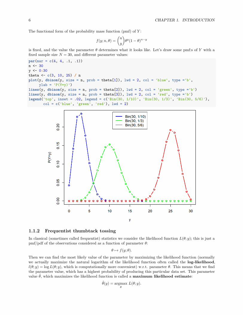
The functional form of the probability mass function (pmf) of Y :
f(y;n, θ) =(n
y
)θy(1− θ)n−y
is fixed, and the value the parameter θ determines what it looks like. Let’s draw some pmf:s of Y with afixed sample size N = 30, and different parameter values:par(mar = c(4, 4, .1, .1))n <- 30y <- 0:30theta <- c(3, 10, 25) / nplot(y, dbinom(y, size = n, prob = theta[1]), lwd = 2, col = 'blue', type ='b',
ylab = 'P(Y=y)')lines(y, dbinom(y, size = n, prob = theta[2]), lwd = 2, col = 'green', type ='b')lines(y, dbinom(y, size = n, prob = theta[3]), lwd = 2, col = 'red', type ='b')legend('top', inset = .02, legend = c('Bin(30, 1/10)', 'Bin(30, 1/3)', 'Bin(30, 5/6)'),
col = c('blue', 'green', 'red'), lwd = 2)
1.1.2 Frequentist thumbtack tossingIn classical (sometimes called frequentist) statistics we consider the likelihood function L(θ; y); this is just apmf/pdf of the observations considered as a function of parameter θ:
θ 7→ f(y; θ).
Then we can find the most likely value of the parameter by maximizing the likelihood function (normallywe actually maximize the natural logarithm of the likelihood function often called the log-likelihood,l(θ; y) = logL(θ; y), which is computationally more convenient) w.r.t. parameter θ. This means that we findthe parameter value, which has a highest probability of producing this particular data set. This parametervalue θ, which maximizes the likelihood function is called a maximum likelihood estimate:
θ(y) = argmaxθ
L(θ; y).
1.1. MOTIVATING EXAMPLE : THUMBTACK TOSSING 7
The maximum likelihood estimate is the most likely value of the parameter given the data.
Let’s derive the maximum likelihood estimate for our binomial model. Because logarithm is a monotonuslyincreasing function, the global maximum point of the log-likelihood maximizes also the likelihood function.Log-likelihood for this model is:
l(θ; y) = log f(y; θ) ∝ log(θy(1− θ)n−y) = y log θ + (n− y) log(1− θ)
We dropped the normalizing constant(ny
)from the likelihood function because it is a constant w.r.t. parameter
θ, and thus has no effect on the maximum point. Next we will find the critical points of the log-likelihood byderivating it w.r.t. θ, and solving the points where the derivative is zero:
l′(θ; y) = y
θ− n− y
1− θ = 0
θ = y
n.
We can see that this indeed is a maximum point by examining the value of the derivative on the both sides ofthis point (it changes from positive to negative), or if we are too lazy to think, by just computing the secondderivative of the log-likelihood:
l′′(θ; y) = − y
θ2 −n− y
(1− θ)2 .
Because 0 ≤ y ≤ n, this is always negative; thus, log-likelihood is a concave function and so its only criticalpoint must be its global maximum point. This means that the maximum likelihood estimate of our model is
θ(y) = y
n= 16
30 ,
which also matches our intuitive solution. But the most likely value is not enough for us: we also wantto know on the other hand how confident we are in our estimate, and on the other hand how likely areother parameter values (besides of the maximum likelihood estimate). We could for example ask what is theprobability that the true value of the parameter lies between 0.4 and 0.6? Or what is the probability that thetrue value of the parameter is higher than 0.5? Or how much more probable it is that the true value of theparameter is higher than 0.5 than it is smaller than 0.5?
Somewhat surprisingly, it turns out that in the framework of classical statistics we cannot directly answerthese questions: they are not considered well-defined! This is because in classical statistics the parameter θis considered as a fixed, but unknown constant. There is nothing random about the parameter; hence wecannot make any probability statements about it.
In classical statistics the way to get around this restriction is to examine the values of the maximum likelihoodestimate over all possible data sets that could have been observed. For instance, we can examine a maximumlikelihood estimate as the function of the random variable Y instead of the observed data y. The resultingrandom variable is called a maximum likelihood estimator (MLE):
θ(Y ) = Y
n.
We can for example estimate the standard deviation of the maximum likelihood estimator (called standarderror). It is also possible to construct confidence intervals for the parameter values: for example 95%confidence interval is an interval (a(Y ), b(Y )), which has at least 95% probability of containing the trueparameter value. Notice that here the randomness is over the observations, not the parameter value.
In the frequentist framework we can also test a so called null hypotesis concerning the parameter value, suchas H0 : θ = 0.5 against an alternative hypothesis H1 : θ 6= 0.5. Again, we do not make any probabilitystatements about the parameter value, but we assume that true value of the parameter is 0.5, and examinehow probable it would be to observe our current data set y with that parameter value.
If all this sounds quite complicated, don’t worry: this is not what we are going to do in this course. Instead,the topic of this course is Bayesian statistical inference. Bayesian framework is conceptually simpler
8 CHAPTER 1. INTRODUCTION
than the classical framework, because we actually can make probability statements about the parametervalues. In Bayesian inference we consider the parameter to be a random variable instead of the fixed constant.Let’s make this explicit by denoting the parameter by capital letter Θ instead of θ.
1.1.3 Fully Bayesian modelAfter this short digression into the frequentist stastics let’s move back to our thumbtack tossing example.What is our proobability estimate for the thumbtack landing point up before we have made any throws?Unlike in coin tossing or the dice throwing, we do not have a clear prior opinion about the possibility of theoutcomes. So let’s make an assumption that all values are equally likely for the probability Θ (the probabilityof thumbtack landing point up). Because Θ is a probability it resides in the interval [0, 1]. Thus, we canquantify our uncertainty about the true parameter value before conducting the experiment by saying that ithas an uniform distribution over the interval [0, 1]:
Θ ∼ U(0, 1).
This is called the prior distribution, and it is a second of the two components required to fully define aBayesian stastical model.
The first component of the Bayesian model, which we have already defined, is the distribution of the datagiven the parameter; this is usually called a sampling distribution or a likelihood. Because in Bayesianinference the parameter is thought as a random variable, let’s change the notation for the sampling distributiona little bit:
fY |Θ(y|θ).From this notation it is clear that the sampling distribution is a conditional probability distribution.
To recap, our full Bayesian model for the thumptack tossing is:
Y |Θ ∼ Bin(n,Θ)Θ ∼ U(0, 1),
and we observed a data set y = 16.
The next step of the Bayesian inference is to update our beliefs about the probability of the parameter valuesafter observing the data. This is quantified by computing the posterior distribution of the parameter Θ.This is simply a conditional distribution of Θ given the data Y = y.
Thus, our task is to find out a conditional distribution fΘ|Y (θ|y) given the model and the observed data.From the probability calculus we remember the chain rule:
fX,Y = fXfY |X ,
which we can use to factorize the joint distribution of the parameter and the data:
fΘ,Y (θ, y) = fY (y)fΘ|Y (θ|y).
Using this factorization we can write the posterior distribution as a quotient of the joint distribution and themarginal distribution of the data:
fΘ|Y (θ|y) = fΘ,Y (θ, y)fY (y)
We can utilize the chain rule again to write the joint distribution as the product of the prior distribution andthe likelihood; hence we can write the posterior distribution as:
fΘ|Y (θ|y) =fΘ(θ)fY |Θ(y|θ)
fY (y)
We have just deduced Bayes’s theorem, which is the cornestone of Bayesian inference! Our model definesthe numerator, so the only unknown component left is the denominator, which is the marginal distribution of
1.1. MOTIVATING EXAMPLE : THUMBTACK TOSSING 9
the data (usually called a marginal likelihood). But luckily we can observe that the posterior distributionis a function of the parameter θ, and there is no θ in the denominator. This means that the denominator is aconstant w.r.t. θ; because we know that the posterior distribution is a probability distribution we can solve itup to the constant term, and deduce the normalizing constant later. Let’s write a posterior distribution asproportional (The proportionality notation f(x) ∝ h(x) means simply that there exists a constant c ∈ R, s.t.f(x) = ch(x)) to the joint distribution:
fΘ|Y (θ|y) ∝ fΘ(θ)fY |Θ(y|θ) = 1 ·(n
y
)θy(1− θ)n−y.
By dropping again drop all the constant terms from this expression, we can simply write:
fΘ|Y (θ|y) ∝ θy(1− θ)n−y.
Is there any probability distribution whose density has this kind of functional form over the interval (0, 1)?Luckily (or later we find out that this was was not such a coincidence after all) it turns out that there indeedis: a beta distribution. Random variable X, which follows a beta distribution with parameters α and β, hasa probability density function
f(x) = 1B(α, β)x
α−1(1− x)β−1,
over interval (0, 1). The integral
B(α, β) = Γ(α)Γ(β)Γ(α+ β) =
∫ 1
0xα−1(1− x)β−1 dx (1.1)
is called a beta function or Euler’s beta function.
We can recognize that the unnormalized posterior distribution is a probability density function of the betadistribution with parameters y+1 and n−y+1 up to a normalizing constant. Hence, our posterior distributionmust be a beta distribution
Θ|Y ∼ Beta(y + 1, n− y + 1).
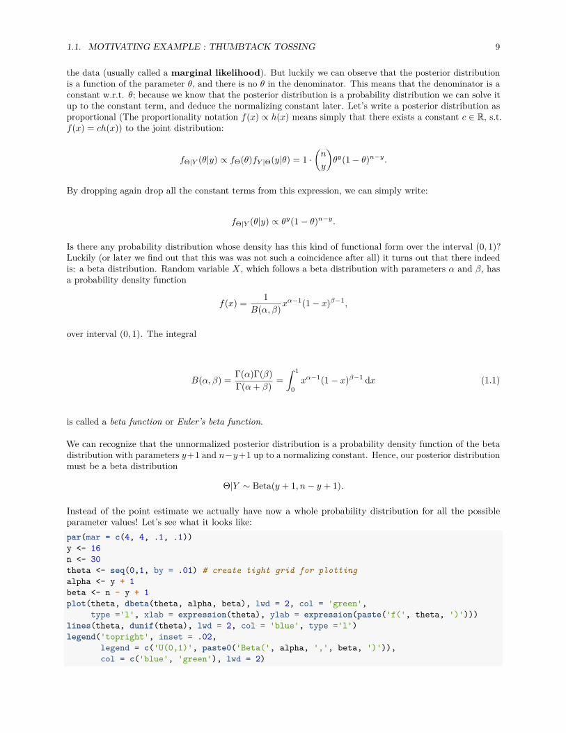
Instead of the point estimate we actually have now a whole probability distribution for all the possibleparameter values! Let’s see what it looks like:par(mar = c(4, 4, .1, .1))y <- 16n <- 30theta <- seq(0,1, by = .01) # create tight grid for plottingalpha <- y + 1beta <- n - y + 1plot(theta, dbeta(theta, alpha, beta), lwd = 2, col = 'green',
type ='l', xlab = expression(theta), ylab = expression(paste('f(', theta, ')')))lines(theta, dunif(theta), lwd = 2, col = 'blue', type ='l')legend('topright', inset = .02,
legend = c('U(0,1)', paste0('Beta(', alpha, ',', beta, ')')),col = c('blue', 'green'), lwd = 2)
10 CHAPTER 1. INTRODUCTION
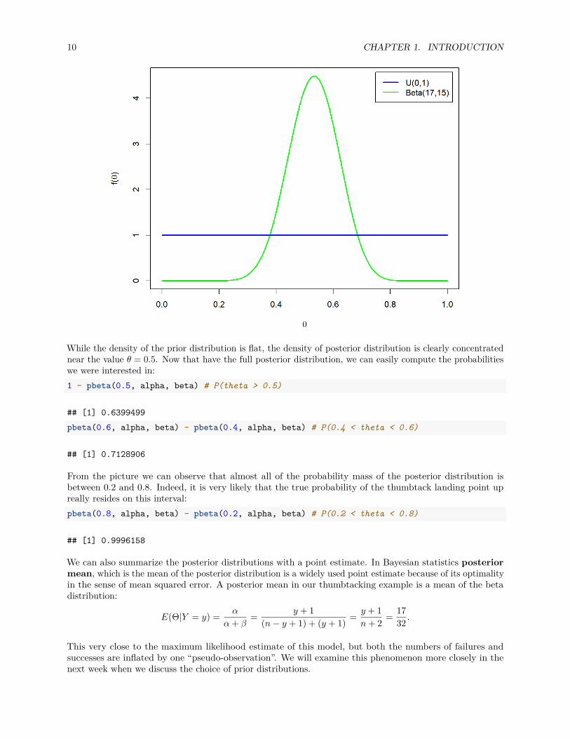
While the density of the prior distribution is flat, the density of posterior distribution is clearly concentratednear the value θ = 0.5. Now that have the full posterior distribution, we can easily compute the probabilitieswe were interested in:1 - pbeta(0.5, alpha, beta) # P(theta > 0.5)
## [1] 0.6399499pbeta(0.6, alpha, beta) - pbeta(0.4, alpha, beta) # P(0.4 < theta < 0.6)
## [1] 0.7128906
From the picture we can observe that almost all of the probability mass of the posterior distribution isbetween 0.2 and 0.8. Indeed, it is very likely that the true probability of the thumbtack landing point upreally resides on this interval:pbeta(0.8, alpha, beta) - pbeta(0.2, alpha, beta) # P(0.2 < theta < 0.8)
## [1] 0.9996158
We can also summarize the posterior distributions with a point estimate. In Bayesian statistics posteriormean, which is the mean of the posterior distribution is a widely used point estimate because of its optimalityin the sense of mean squared error. A posterior mean in our thumbtacking example is a mean of the betadistribution:
E(Θ|Y = y) = α
α+ β= y + 1
(n− y + 1) + (y + 1) = y + 1n+ 2 = 17
32 .
This very close to the maximum likelihood estimate of this model, but both the numbers of failures andsuccesses are inflated by one “pseudo-observation”. We will examine this phenomenon more closely in thenext week when we discuss the choice of prior distributions.
1.2. COMPONENTS OF BAYESIAN INFERENCE 11
1.2 Components of Bayesian inferenceLet’s briefly recap and define more rigorously the main concepts of the Bayesian belief updating process,which we just demonstrated.
Consider a slightly more general situation than our thumbtack tossing example: we have observed a dataset y = (y1, . . . , yn) of n observations, and we want to examine the mechanism which has generated theseobservations. To this end, we model the observed data set as an observed value of the random vectorY = (Y1, . . . , Yn).
In this course we limit ourselves to the parametric inference. Parametric inference is a special case of thestatistical inference where it is assumed that the functional form of the joint distribution of the random vectorY is fixed up to the value of the parameter vector θ = (θ1, . . . , θd) ∈ Ω living in some parameter spaceΩ. The distribution of the data is written as the conditional distribution of the data given the parameter(because, as we remember, in Bayesian inference the parameter is considered as a random variable): fY|Θ(y|θ).This means that inference about the distribution of the data is reduced to finding out the distribution of theunknown parameter Θ. This simplifies the inference process significantly, because we can limit ourselves tothe vector spaces instead of the function spaces.
Sampling distribution / likelihood functionConditional distribution of the data set given the parameter, fY|Θ(y|θ), is called a sampling distribution, orthe often simply a likelihood function.
More rigorously the sampling distribution means fY|Θ(y|θ) as a function of the observed data:
y 7→ fY|Θ(y|θ),
and likelihood function as a function of the parameter:
θ 7→ fY|Θ(y|θ),
but often these terms are used interchangeably in practice (and also on this course).
Because our data set is a vector, in the general case a structure of the sampling distribution can be quitecomplicated. However, if we assume that our observations are independent (given the value of the parameterΘ), denoted as
Y1, . . . , Yn ⊥⊥ |Θ,
the joint sampling distribution of random vector Y can be factorized into a product of the samplingdistributions of its components:
fY|Θ(y|θ) =n∏i=1
fYi|Θ(yi|θ).
The situation is further simplified if our observations follow a same distribution. This situation is encounteredquite often in this course, at least in the simplest examples. We say that random variables are independentand identically distributed (i.i.d.). In this case each of n components of the random vector Y has acommon sampling distribution f(y|θ), and the joint sampling distribution can be further simplified to
fY|Θ(y|θ) =n∏i=1
f(yi|θ).
In some cases, such as in our thumbtack tossing example the form of the sampling distribution (binomialdistribution in this case) follows quite naturally from the structure of the expermintal situation. Otherdistributions that often follow naturally from the symmetry arguments or physical aspects of the examinedphenomenon are multinomial distribution (extension of binomial experiment into the experiments with morethan two possible outcomes, such as throwing a dice), normal distribution (sums or means of the independentrandom variables), Poisson distribution (occurrences of the independent events) and exponential distribution
12 CHAPTER 1. INTRODUCTION
(waiting times or lifespans). In the more complex situations we cannot usually use any of these simple modelsdirectly, but we can try to build so called hierarchical models out of these basic distributions. Ultimatelythe choice of the sampling distribution is subjective, and up to our domain knowledge of the modelledphenomenon / and or computational convenience.
Prior distributionA marginal distribution fΘ(θ) of the parameter is called a prior distribution. Priori is latin for before: theprior distribution describes our beliefs about the likely values of the parameter Θ before observing any data.
If we do not have any strong beliefs about the possible values of the parameter or we do not want let ourbeliefs to influence our results, we should choose as a vague priori distribution as possible, such as theuniform distribution in our thumbtack tossing example. This kind of the priori distribution is called anuninformative prior. But what we mean by “vague” here? It turns out that it is not possible to finda prior distribution that would be universally uninformative. For example uniform priors lead quickly toproblems, if the parameter space is not restriced: how can you even define an uniform distribution over aninterval of infinite length?
On the other hand, when we want to let our prior knowledge influence our posterior distribution, we set astronger prior distribution. This kind of the prior distribution is called an informative prior. Informativeprior distribution may be for example used to enforce sparsity into the model; this means we have a strongprior belief that some parameters of the model should be zero.
We will soon revisit uninformative and informative priors with a simple example.
The prior distribution for the parameter vector Θ is also a parametric distribution; its parameters φ =(φ1, . . . , φk) are called hyperparameters. We can denote prior distribution also as fΘ|Φ(θ|φ), but often thenotation is simplified by leaving out the hyperparameters.
Bayesian modelTo specify the fully Bayesian probability model, besides of the sampling distribution, we also need to specifythe prior distribution of the parameter.
Together they determine the joint distribution of the observed data and the parameter:
fΘ,Y(θ, y) = fΘ(θ)fY|Θ(y|θ).
This full joint distribution is rarely computed or handled explicitly. Instead, the Bayesian inference is basedon computing conditional and marginal densities from it.
Posterior distributionThe conditional distribution of the parameter given the data is called a posterior distribution. Posteriori islatin for after : posterior distribution describes our beliefs about the probable values of the parameter afterwe have observed the data.
In principle, the posterior distribution is computed from the prior and the sampling distributions using theBayes’ theorem:
fΘ|Y(θ|y) = fΘ,Y(θ, y)fY(y) =
fΘ(θ)fY|Θ(y|θ)fY(y) .
In practice, we usually utilize the fact that the normalizing constant fY(y) contains no θ; thus, it is a constantw.r.t. parameter θ. This means that we can compute the unnormalized density of the posterior distributionsimply as a product of the sampling and prior distributions:
fΘ|Y(θ|y) ∝ fΘ(θ)fY|Θ(y|θ),
and then deduce the missing normalizing constant. In the first examples of this course this often done byrecognizing the functional form of the familiar probability density.
1.3. PREDICTION 13
Marginal likelihoodThe normalizing constant fY(y) of the Bayes’ theorem is called a marginal likelihood (sometimes also anevidence). It is computed by marginalizing out the parameter from the full joint probability distribution. Forthe continuous parameter this is done by integrating the joint probability distribution over the parameterspace:
fY(y) =∫
ΩfΘ(θ)fY|Θ(y|θ)dθ,
and for the discrete parameter by summing the joint probability distribution over the parameter space:
fY(y) =∑θ∈Ω
fΘ(θ)fY|Θ(y|θ).
If this averaging over all the possible parameter values seems a strange idea, it is probably easier to understandit by first considering the discrete case. You can for example take a look at the how the denominator of theBayes’ theorem is computed in the classical drug testing example: Bayes’ theorem - Wikipedia.
In Bayesian data analysis Gelman et al. (2013) the marginal likelihood is called a prior predictive distribution.This is because it presents our beliefs about the probabilities of the data before any observations are made. Itis a distribution of the data computed as a weighted average over all the possible parameter values, and theweights are determined by the prior distribution.
If we denoteg(y, θ) := fY|Θ(y|θ),
we can write the marginal likelihood as:
fY(y) =∫
Ωg(y, θ)fΘ(θ)dθ = E[g(y,Θ)], (1.2)
So the marginal likelihood can be written as an expectation of the sampling distribution, where the expectationis taken over the prior distribution of the parameter Θ! Again, it may be easier to consider first a case of adiscrete parameter, where the expectation is actually computed as an weighted average.
1.3 Prediction1.3.1 Motivating example, part IILet’s revisit the thumbtack tossing example: assume we have tossed a thumbtack n = 30 times, and observedthat it has landed point up y = 16 times. But oftentimes instead of making inference about the parametersof the model, we are actually more interested in predicting the new observations. So what is our predictivedistribution for the number of successes, if we throw the same thumbtack m = 10 more times?
Because the thumbtack stays the same, it makes sense to model the new throws as a sample from the samebinomial distribution with the same successes probability as the original observations:
Y ∼ Bin(m,Θ)
Further, it makes sense to model the old and the new observations independent given the parameter:
Y , Y ⊥⊥ |Θ.
A naive way to obtain a probability mass function of Y would be just to plug the point estimate, such as amaximum likelihood estimate θMLE(y), as the parameter value of the probability mass function of the newobservations: fY |Θ(y|θMLE(y)). However, by identifying the success probability the observed proportion ofthe successes, we run into the same problems as in the case of the parameter estimation: what if we hadagain observed a data y = 0 with n = 3? Then the predictive distribution would assing a probability 1 to the
14 CHAPTER 1. INTRODUCTION
value Y = n, and probability 0 to all the other values. Surely we would have not needed any statistics toarrive at the conclusion that the thumbtack will land point down every time!
Instead, we will derive the proper Bayesian predictive distribution by actually computing the probability ofthe new observations given the observed data! This is denoted by fY |Y (y|y). We can immediately observethat the parameter theta does not exist at all in this formula. However, to derive the predictive distribution,we include the parameter as an auxiliary variable that is then integrated out. We first specify the jointdistribution of the new observation y and the parameter θ given the observed data y, and then get thepredictive distribution by integrating over the parameter space:
fY |Y (y|y) =∫
ΩfY ,Θ|Y (y|y)dθ
=∫
ΩfY |Θ,Y (y|θ, y)fΘ|Y (θ|y)dθ
=∫
ΩfY |Θ(y|θ)fΘ|Y (θ|y)dθ.
(1.3)
In the second equality we used a chain rule for the conditional probabily densities:
fX,Y |Z = fX|Y,Z fY |Z ,
and in the final equality used a fact that the new observations are independent of the observed data given theparameter to simplify the expression. This predictive distribution fY |Y (y|y) of the new observations giventhe data we just derived is known as a posterior predictive distribution.
Now that we derived a general form of the posterior predictive distribution, we can plug the samplingdistribution of the new observations fY |Θ(y|θ) and the posterior distribution fΘ|Y (θ|y) we derived in the partone of this example, into this formula:
fY |Y (y|y) =∫
ΩfY |Θ(y|θ)fΘ|Y (θ|y)dθ
=∫ 1
0
(m
y
)θy(1− θ)m−y 1
B(α1, β1)θα1−1(1− θ)β1−1 dθ
=(m
y
)1
B(α1, β1)
∫ 1
0θy+α1−1(1− θ)m+β1−y−1 dθ.
To simplify the notation, we have denoted the parameters of the posterior distribution as α1 = y + 1, andβ1 = n− y + 1.
Next we are going to integrate in “a statistician way”: this means that we are not going to really integratethe expression, but we get rid of it by recognizing it as the integral whose value we know. We can do this byusing one of the following tricks:
1. Explicitly recognize a familiar integral : We can immediately observe that the integral is a betafunction (see eq. (1.1)), so we can write it more concisely as:∫ 1
0θy+α1−1(1− θ)m+β1−y−1 dθ = B(y + α1,m+ β1 − y).
2. Recognize an unnormalized probability density function of the familiar distribution : Wecan also immediately observe that the integrand is a probability density function of the beta distributionBeta(y+α1,m+β1− y) up to a normalizing constant, and it is integrated over the support of the distribution.This means that if we add the missing normalizing constant, the integral is an integral of the probability
1.3. PREDICTION 15
density over its support:
∫ 1
0θy+α1−1(1− θ)m+β1−y−1 dθ
=B(y + α1,m+ β1 − y)∫ 1
0
1B(y + α1,m+ β1 − y)θ
y+α1−1(1− θ)m+β1−y−1 dθ
= B(y + α1,m+ β1 − y) · 1= B(y + α1,m+ β1 − y).
In this case the first trick was more straight-forward, but I also introduced the second one because in somecases recognizing the familiar integral requires performing a change of variables, and an unnormalized densityfunction of the familiar distribution may be easier to recognize.
Whichever of these tricks you use, the posterior predictive distribution is simplified to
fY |Y (y|y) =(m
y
)B(y + α1,m+ β1 − y)
B(α1, β1) .
This a is probability distribution of the so called beta-binomial distribution, so we can denote our posteriorpredictive distribution as
Y |Y ∼ Beta-bin(m,α1, β1),
where α1 = y + 1, and β1 = n− y + 1 are the parameters of the posterior distribution for the parameter Θ.
1.3.2 Posterior predictive distribution
Let’s consider a general case: assume we have observations Y = (Y1, . . . , Yn) with a sampling distributionfY|Θ(y|θ) conditional on the unknown parameter vector Θ ∈ Ω. Now we want to predict the distribution forthe m new observations Y = (Y1, . . . , Ym) from the same process. Distribution
fY|Y(y|y)
of the new observations given the observed data is called a posterior predictive distribution. If we furthermake a simplifying assumption that the new observations are independent of the observed data given theparameter, written as:
Y,Y |Θ,
we can write the posterior predictive distribution as an integral
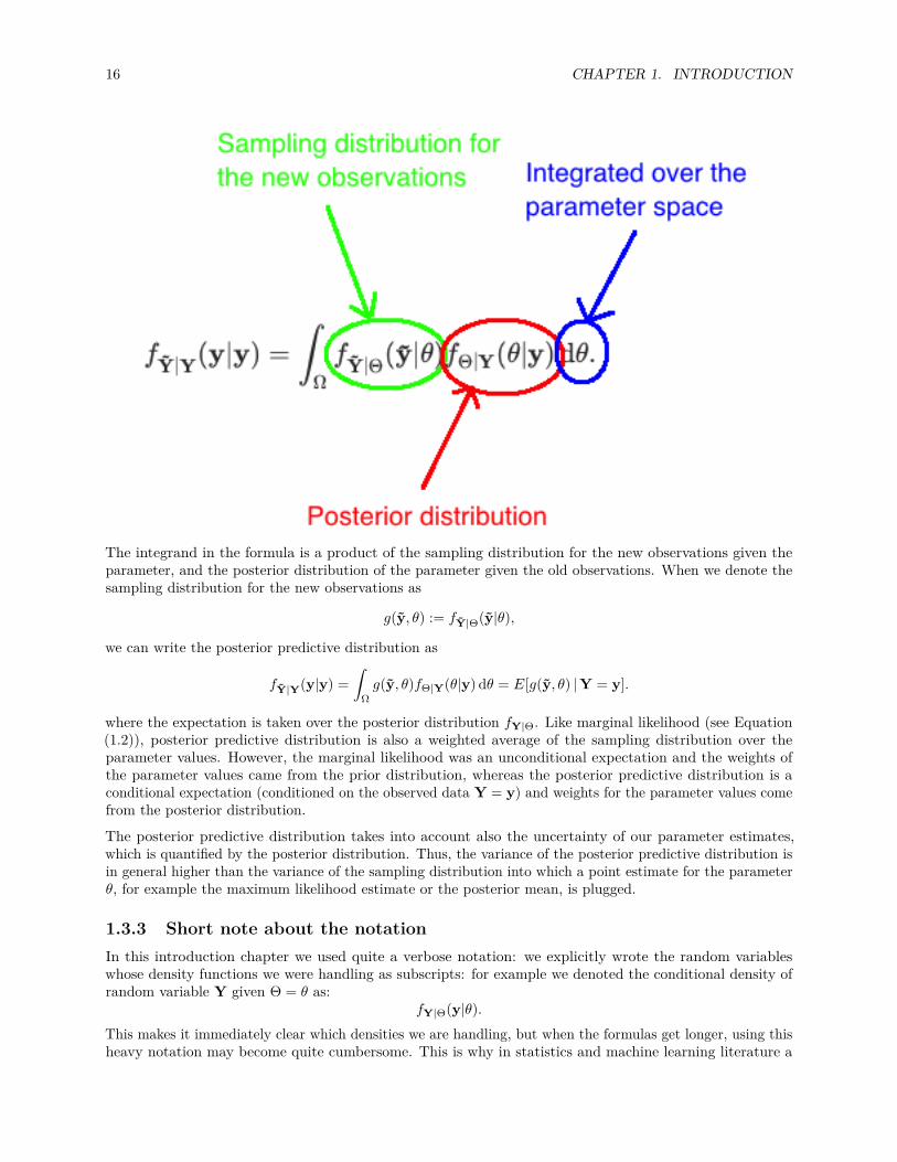
fY|Y(y|y) =∫
ΩfY|Θ(y|θ)fΘ|Y(θ|y)dθ,
which we derived in Equation (1.3). This formula may seem a little bit intimidating at first, but let’s try tofind the intuition behind it.
16 CHAPTER 1. INTRODUCTION
The integrand in the formula is a product of the sampling distribution for the new observations given theparameter, and the posterior distribution of the parameter given the old observations. When we denote thesampling distribution for the new observations as
g(y, θ) := fY|Θ(y|θ),
we can write the posterior predictive distribution as
fY|Y(y|y) =∫
Ωg(y, θ)fΘ|Y(θ|y)dθ = E[g(y, θ) |Y = y].
where the expectation is taken over the posterior distribution fY|Θ. Like marginal likelihood (see Equation(1.2)), posterior predictive distribution is also a weighted average of the sampling distribution over theparameter values. However, the marginal likelihood was an unconditional expectation and the weights ofthe parameter values came from the prior distribution, whereas the posterior predictive distribution is aconditional expectation (conditioned on the observed data Y = y) and weights for the parameter values comefrom the posterior distribution.
The posterior predictive distribution takes into account also the uncertainty of our parameter estimates,which is quantified by the posterior distribution. Thus, the variance of the posterior predictive distribution isin general higher than the variance of the sampling distribution into which a point estimate for the parameterθ, for example the maximum likelihood estimate or the posterior mean, is plugged.
1.3.3 Short note about the notationIn this introduction chapter we used quite a verbose notation: we explicitly wrote the random variableswhose density functions we were handling as subscripts: for example we denoted the conditional density ofrandom variable Y given Θ = θ as:
fY|Θ(y|θ).This makes it immediately clear which densities we are handling, but when the formulas get longer, using thisheavy notation may become quite cumbersome. This is why in statistics and machine learning literature a

1.3. PREDICTION 17
more concise notation is generally used. In this slight abuse of notation all the density and probability massfunctions are denoted with the same letter (usually p) without any subscripts. The random variables whosedensity functions they are can be recognized by the arguments of the densities. For example the conditionaldensity fY|Θ(y|θ) is written concisely as p(y|θ), and the Bayes’ theorem can be written as
p(θ|y) = p(θ)p(y|θ)p(y) .
This shorthand notation makes formulas shorter and more clear to read assuming that you know in the firstplace for which it is shorthand for. In the following chapters we will use this notation.
Often also the random variables and their realizations are denoted with the same lowercase letter if thereis no risk of confusion. This is particularly the case with the parameters, in part because there exist nouseful uppercase versions of many greek alphabets. So when we talk about “the parameter θ” in the followingchapters, you have to remember that usually a random variable is meant.

18 CHAPTER 1. INTRODUCTION
Chapter 2
Conjugate distributions
Conjugate distribution or conjugate pair means a pair of a sampling distribution and a prior distributionfor which the resulting posterior distribution belongs into the same parametric family of distributions than theprior distribution. We also say that the prior distribution is a conjugate prior for this sampling distribution.
A parametric family of distributionsfY |Θ(y|θ) : θ ∈ Ω
means simply a set of distributions which have a same functional form, and differ only by the value of thefinite-dimensional parameter θ ∈ Ω. For instance, all beta distributions or all normal distributions form aparametric families of distributions.
We have already seen one example of the conjugate pair in the thumbtack tossing example: the binomial andthe beta distribution. You may now be wondering: “But Ville, in our example the prior distribution was anuniform distribution, not a beta distribution??” It turns out that the prior was indeed a beta distribution,because the uniform distribution U(0, 1) is actually a same distribution than the beta distribution Beta(1, 1)(check that this holds!).
Using conjugate pairs of distributions makes a life of the statistician more convenient, because the marginallikelihood, and thus also the posterior distribution and the posterior predictive distribution can be solved ina closed form. Actually, it turns out that this is the second of the only two special cases in which this ispossible:
1. The parameter space is discrete and finite: Ω = (θ1, . . . , θp); in this case the marginal likelihood can becomputed as a finite sum:
fY (y) =p∑i=1
fY|Θ(yi|θi)fΘ(θi).
2. The prior distribution is a conjugate prior for the sampling distribution.
In all the other cases we have to approximate the posterior distributions and the posterior predictivedistributions. Usually this is done by simulating values from them; we will return to this topic soon.
2.1 One-parameter conjugate modelsWhen parameter Θ ∈ Ω is a scalar, the inference is particularly simple. We have already seen one example ofthe one-parameter conjugate model (the thumbtacking example), but let’s examine another simple model.
2.1.1 Example: Poisson-gamma modelA Poisson distribution is a discrete distribution which can get any non-negative integer values. It is a naturaldistribution for modelling counts, such as goals in a football game, or a number of bicycles passing a certain
19
20 CHAPTER 2. CONJUGATE DISTRIBUTIONS
point of the road in one day. Both the expected value and the variance of a Poisson distributed randomvariable are equal to the parameter of the distribution: if Y ∼ Poisson(λ),
E[Y ] = λ, V ar[Y ] = λ.
Let’s cheat a little bit this time: we will first generate observations from the distribution with a knownparameter, and then try estimate the posterior distribution of the parameter from this data:n <- 5lambda_true <- 3
# set seed for the random number generator, so that we get replicable resultsset.seed(111111)y <- rpois(n, lambda_true)y
## [1] 4 3 11 3 6
Now we actually know that the true generating distribution of our observations y = (4, 3, 11, 3, 6) is Poisson(3);but lets forget this for a moment, and proceed with the inference.
Assume that the observed variables are counts, which means that they can in principle take any non-negativeinteger value. Thus, it is natural to model them as independent Poisson-distributed random variables:
Y1, . . . , Yn ∼ Poisson(λ) ⊥⊥ |λ
Because the parameter of the Poisson distribution can in principle be any positive real number, we want usea prior whose support is (0,∞). If we used for example an uniform prior U(0, 100), posterior density wouldalso be zero outside of this interval, even if all the observations were greater than 100. So usually we want aprior that assings a non-zero density for all the possible parameter values.
It is not possible to set a uniform distribution over the infinite interval (0,∞), so we have to come up withsomething else. A gamma distribution is a convenient choice. It is a distribution with a peak close to zero,and a tail that goes to infinity. It also turns out that the gamma distribution is a conjugate prior for thePoisson distribution: this means tha we can actually solve the posterior distribution in a closed form.
We can set the parameters of the prior distribution for example to α = 1 and β = 1; we will examine thechoice of both the prior distribution and its parameters (called hyperparameters) later. For now on, let’s justsolve the posterior with the conjugate gamma prior:
λ ∼ Gamma(α, β).
Because the observations are independent given the parameter, a likelihood function for all the observationsY = (Y1, . . . , Yn) can be written as a product of the Poisson distributions:
p(y|λ) =n∏i=1
p(yi|λ) =n∏i=1
λyie−λ
yi!∝ λ
∑n
i=1yie−nλ = λnye−nλ,
where
y = 1n
n∑i=1
yi
is a mean of the observations. Again we dropped the constant terms which do not depend on the parameterfrom the expression of the likelihood.
The unnormalized posterior distribution for the parameter λ can now be written as
2.1. ONE-PARAMETER CONJUGATE MODELS 21
p(λ|y) ∝ p(y|λ)p(λ)∝ λnye−nλλα−1e−βλ
= λα+ny−1e−(β+n)λ.
(2.1)
The gamma prior was chosen because a gamma distribution is a conjugate prior for the Poisson distribution,and indeed we can recognize the unnormalized posterior distribution as the kernel of the gamma distribution.Thus, the posterior distribution is
λ |Y ∼ Gamma(α+ ny, β + n).
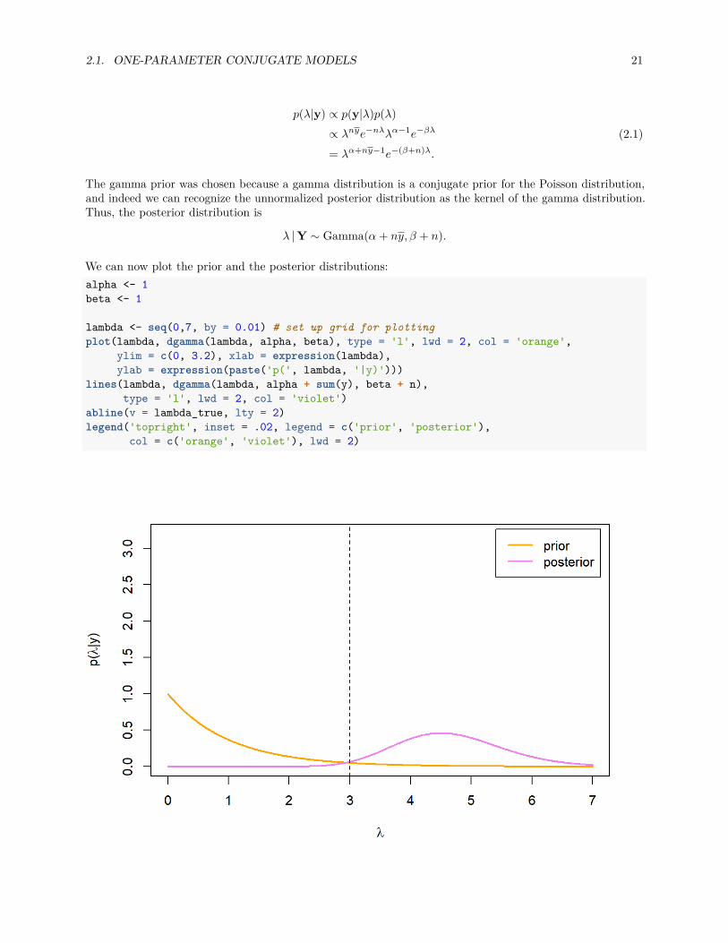
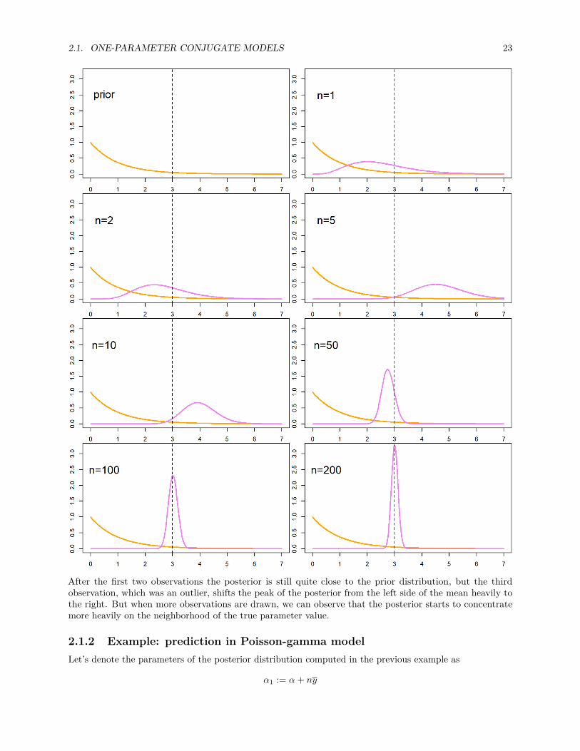
We can now plot the prior and the posterior distributions:alpha <- 1beta <- 1
lambda <- seq(0,7, by = 0.01) # set up grid for plottingplot(lambda, dgamma(lambda, alpha, beta), type = 'l', lwd = 2, col = 'orange',
ylim = c(0, 3.2), xlab = expression(lambda),ylab = expression(paste('p(', lambda, '|y)')))
lines(lambda, dgamma(lambda, alpha + sum(y), beta + n),type = 'l', lwd = 2, col = 'violet')
abline(v = lambda_true, lty = 2)legend('topright', inset = .02, legend = c('prior', 'posterior'),
col = c('orange', 'violet'), lwd = 2)
22 CHAPTER 2. CONJUGATE DISTRIBUTIONS
We can see that the posterior distribution is concentrated quite a bit higher than the true parameter value.This is because our third observation happened to be a bit of an outlier: the probability of drawing a value of11 or higher from Poisson(3)-distribution (if we draw only one value), is only:ppois(10,3, lower.tail = FALSE)
## [1] 0.000292337
But because we are anyway using simulated data, let’s draw some more observations from the same Poisson(3)-distribution:n_total <- 200set.seed(111111) # use same seed, so first 5 obs. stay samey_vec <- rpois(n_total, lambda_true)head(y_vec)
## [1] 4 3 11 3 6 3
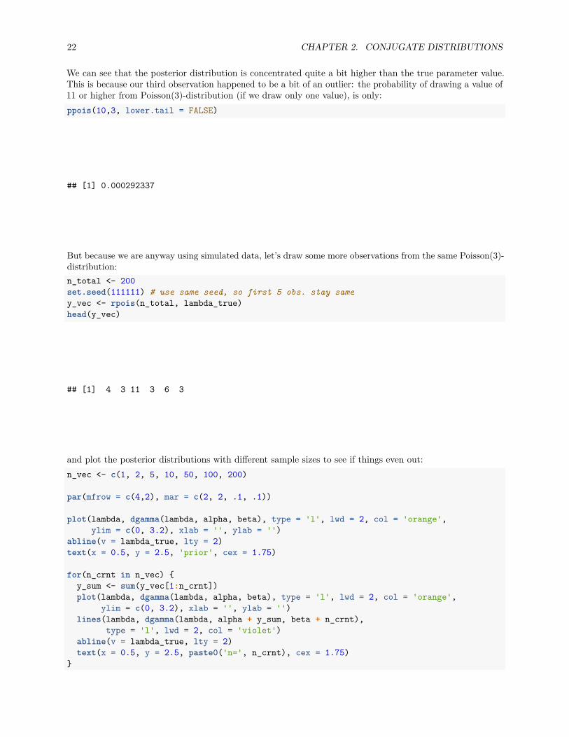
and plot the posterior distributions with different sample sizes to see if things even out:n_vec <- c(1, 2, 5, 10, 50, 100, 200)
par(mfrow = c(4,2), mar = c(2, 2, .1, .1))
plot(lambda, dgamma(lambda, alpha, beta), type = 'l', lwd = 2, col = 'orange',ylim = c(0, 3.2), xlab = '', ylab = '')
abline(v = lambda_true, lty = 2)text(x = 0.5, y = 2.5, 'prior', cex = 1.75)
for(n_crnt in n_vec) y_sum <- sum(y_vec[1:n_crnt])plot(lambda, dgamma(lambda, alpha, beta), type = 'l', lwd = 2, col = 'orange',
ylim = c(0, 3.2), xlab = '', ylab = '')lines(lambda, dgamma(lambda, alpha + y_sum, beta + n_crnt),
type = 'l', lwd = 2, col = 'violet')abline(v = lambda_true, lty = 2)text(x = 0.5, y = 2.5, paste0('n=', n_crnt), cex = 1.75)
2.1. ONE-PARAMETER CONJUGATE MODELS 23
After the first two observations the posterior is still quite close to the prior distribution, but the thirdobservation, which was an outlier, shifts the peak of the posterior from the left side of the mean heavily tothe right. But when more observations are drawn, we can observe that the posterior starts to concentratemore heavily on the neighborhood of the true parameter value.
2.1.2 Example: prediction in Poisson-gamma modelLet’s denote the parameters of the posterior distribution computed in the previous example as
α1 := α+ ny
24 CHAPTER 2. CONJUGATE DISTRIBUTIONS
andβ1 := β + n,
and solve the posterior predictive distribution for one new observation Y1 from the same Poisson distributionas the observed data:
Y1, Y1, . . . , Yn ∼ Poisson(λ) ⊥⊥ |λ.
The posterior predictive distribution for Y1 can be written as:
p(y1|y) =∫
Ωp(y1|λ)p(λ|y)dλ
=∫ ∞
0λy1
e−λ
y1!βα1
1Γ(α1)λ
α1−1e−β1λ dλ
= βα11
Γ(α1)y1!
∫ ∞0
λy1+α1−1e−(β1+1)λ dλ.
Now it would be probably easiest to use the first of the tricks introduced in Example 1.3.1, and complete theintegral into an integral of a gamma density over its support. But just to make things more interesting, let’suse the second trick by completing it into a gamma function by the following change of variables:
t = (β1 + 1)λ.
Nowλ = g(t) := t
β1 + 1 ,
anddλ = g′(t)dt = 1
β1 + 1 dt.
This change of variables is only a multiplication by a positive constant, so it has no effect on the limits of theintegral. After performing the change of variables we can recognize the gamma integral:∫ ∞
0λy1+α1−1e−(β1+1)λ dλ =
∫ ∞0
(t
β1 + 1
)y1+α1−1e−t
1β1 + 1 dt
=(
1β1 + 1
)y1+α1 ∫ ∞0
ty1+α1−1e−t dt
=(
1β1 + 1
)y1+α1
Γ(y1 + α1).
Thus, we can write the posterior predictive density as
p(y1|y) = βα11
Γ(α1)y1! ·(
1β1 + 1
)y1+α1
Γ(y1 + α1)
= Γ(y1 + α1)Γ(α1)y1!
(1
β1 + 1
)y1 ( β1
β1 + 1
)α1
= Γ(y1 + α1)Γ(α1)y1!
(1− β1
β1 + 1
)y1 ( β1
β1 + 1
)α1
.
This is a density function of the following negative binomial distribution:
Y1 |Y ∼ Neg-Bin(α1,
β1
β1 + 1
).
Still assuming that our prior was Gamma(1, 1)-distribution, we can compare this posterior predictivedistribution to the true generative distribution of the data:
2.1. ONE-PARAMETER CONJUGATE MODELS 25
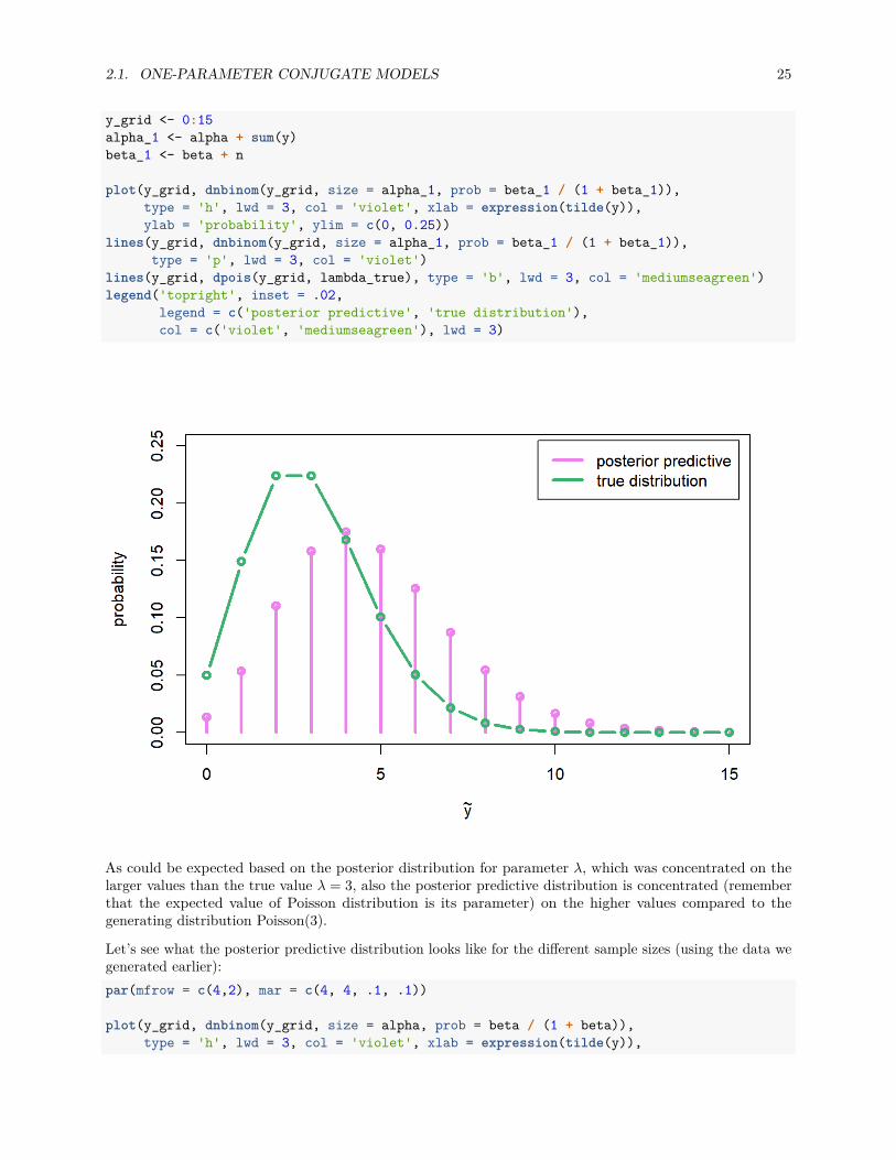
y_grid <- 0:15alpha_1 <- alpha + sum(y)beta_1 <- beta + n
plot(y_grid, dnbinom(y_grid, size = alpha_1, prob = beta_1 / (1 + beta_1)),type = 'h', lwd = 3, col = 'violet', xlab = expression(tilde(y)),ylab = 'probability', ylim = c(0, 0.25))
lines(y_grid, dnbinom(y_grid, size = alpha_1, prob = beta_1 / (1 + beta_1)),type = 'p', lwd = 3, col = 'violet')
lines(y_grid, dpois(y_grid, lambda_true), type = 'b', lwd = 3, col = 'mediumseagreen')legend('topright', inset = .02,
legend = c('posterior predictive', 'true distribution'),col = c('violet', 'mediumseagreen'), lwd = 3)
As could be expected based on the posterior distribution for parameter λ, which was concentrated on thelarger values than the true value λ = 3, also the posterior predictive distribution is concentrated (rememberthat the expected value of Poisson distribution is its parameter) on the higher values compared to thegenerating distribution Poisson(3).
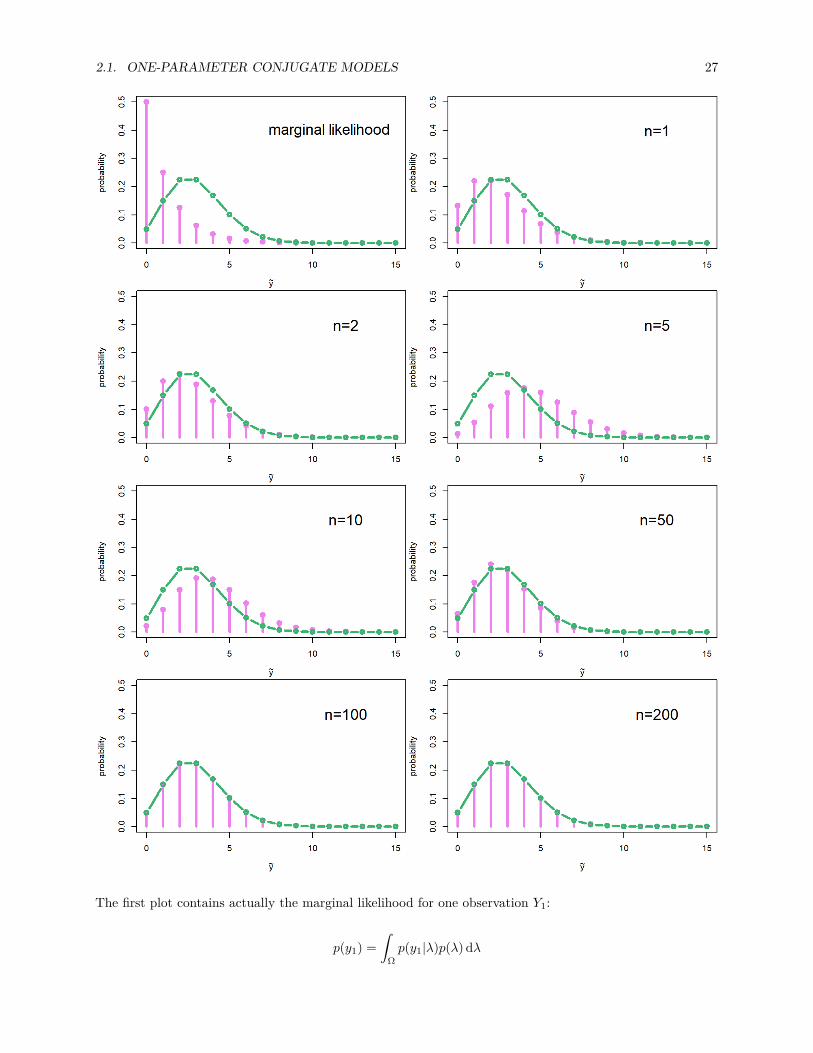
Let’s see what the posterior predictive distribution looks like for the different sample sizes (using the data wegenerated earlier):par(mfrow = c(4,2), mar = c(4, 4, .1, .1))
plot(y_grid, dnbinom(y_grid, size = alpha, prob = beta / (1 + beta)),type = 'h', lwd = 3, col = 'violet', xlab = expression(tilde(y)),
26 CHAPTER 2. CONJUGATE DISTRIBUTIONS
ylab = 'probability', ylim = c(0, 0.5))lines(y_grid, dnbinom(y_grid, size = alpha, prob = beta / (1 + beta)),
type = 'p', lwd = 3, col = 'violet')lines(y_grid, dpois(y_grid, lambda_true), type = 'b', lwd = 3, col = 'mediumseagreen')text(x = 11, y = 0.4, 'marginal likelihood', cex = 1.75)
for(n_crnt in n_vec) y_sum <- sum(y_vec[1:n_crnt])alpha_1 <- alpha + y_sumbeta_1 <- beta + n_crntplot(y_grid, dnbinom(y_grid, size = alpha_1, prob = beta_1 / (1 + beta_1)),
type = 'h', lwd = 3, col = 'violet', xlab = expression(tilde(y)),ylab = 'probability', ylim = c(0, 0.5))
lines(y_grid, dnbinom(y_grid, size = alpha_1, prob = beta_1 / (1 + beta_1)),type = 'p', lwd = 3, col = 'violet')
lines(y_grid, dpois(y_grid, lambda_true), type = 'b', lwd = 3, col = 'mediumseagreen')text(x = 12, y = 0.4, paste0('n=', n_crnt), cex = 1.75)
2.1. ONE-PARAMETER CONJUGATE MODELS 27
The first plot contains actually the marginal likelihood for one observation Y1:
p(y1) =∫
Ωp(y1|λ)p(λ)dλ
28 CHAPTER 2. CONJUGATE DISTRIBUTIONS
This marginal likelihood is Neg-bin(α, β
β+1
)-distribution. We already basicly derived this when we computed
the posterior predictive distribution; the only difference was in the parameters of the gamma distribution.This also holds in a more general case: the derivation for the marginal likelihood and the posterior predictivedistribution is the same; the only difference is in the value of the parameters of the conjugate prior distribution.This means that every time we can solve the posterior distribution in a closed form, we can also solve theposterior predictive distribution!
But I digress. . . Let’s look at the plots again: when we have only one or two observations, the posteriorpredictive distribution is closer to the marginal likelihood. Again, the third observation, which was theoutlier, tilts the posterior predictive distribution immediately towards the higher values, until the it starts toresemble more or less the true generating distribution when more data is generated.
This is recurring theme in a Bayesian inference: when the sample size is small, the prior has more influenceon the posterior, but when the sample size grows, the data starts to influence our posterior distributionmore and more, until at the limit the posterior is determined purely by the data (at least when the certainconditions hold). Examining the case n→∞ is called asymptotics, and it is a cornerstone of the statisticalinference, but we do not have time go very deep into this topic on this course.
Now you may be thinking: “But if have enough data, then we do not have to care about the priors, don’twe?” Well, in this case you are lucky, but before you can forget about the priors, you have to ask yourself (atleast) two things:
1. How complex model you want to fit? In general, more complex the model, more data you need. Forexample modern deep learning models may have millions of parameters, so probably a sample size ofn = 50 is not “high enough”, although this was the case in our toy example.
2. In what resolution level you want examine your data? You may have enough data to fit your modelat the level of the country, but what if you want to model the differences between the towns? Or theneighborhoods? We will actually have a concrete example of this exact situation on the exercises later.
2.2 Prior distributionsThe most often criticized aspect of the Bayesian approach to statistical inference is the requirement to choosea prior distribution, and especially the subjectivity of this prior selection procedure. The Bayesian answer tothis criticism is to point out that the whole modeling procedure is inherently subjective: it is never possiblefor the data to fully “speak for itself” because we have to always make some assumptions about its samplingdistribution.
Even in the most trivial coin-flipping example the choice of the binomial distribution for the outcome of thecoinflip can be questioned: if we were truly ignorant about the outcome of the coinflip, would it make senseto model the outcome with a trinomial distribution, where the outcomes were head, tails and the coin landingon its side? So even the choice of the restricting the parameter space to Ω = heads, tails is based on theour prior knowledge about the previous coinflips and the common sense knowledge that the coin landing onits side is almost impossible. It can be argumented that we always use somehow our prior knowledge in themodelling process, but the Bayesian framework just makes utilizing prior knowledge more transparent andeasier to quantify.
A less philosophical and more practical example of the inherent subjectivity of the modelling process is anysituation in which our observations are continuous instead of the discrete. For instance, let’s consider aclassical statistical problem of estimating the true population distribution of some quantity, say the averageheight of adult females, on the basis of the subsample from some human population. Assume that we havemeasured the following heights of the five people from this population, say some tribe in South America (inmetres):
y = (1.563, 1.735, 1.642, 1.662, 1.528).
Now we could of course “let the data speak for itself”, and assume that the true distribution of the height of
2.2. PRIOR DISTRIBUTIONS 29
the females of this tribe is the empirical distribution of our observations:
P (Y = y) =
1/5 if y = 1.563,1/5 if y = 1.735,1/5 if y = 1.642,1/5 if y = 1.662,1/5 if y = 1.528,0 otherwise.
But this would of course be an absurd conclusion. In practice, we have to impose some kind of the samplingdistribution, for example the normal distribution, for the observations for our inferences to be sensible. Evenif we do not want to impose any parametric distribution on the data, we have to choose some nonparametericmethod to smooth a height distribution.
So this is the Bayesian counter-argument: the choice of the sampling distribution is as subjective as thechoice of the prior distribution. Take for instance a classical linear regression. It makes huge simplifyingassumptions: that the true that the error terms are normally distributed given the predictors, and that theparameters of this normal distribution do not depend on the values of the predictors. Also the choices ofthe predictors inject very strong subjective beliefs into the model: if we exclude some predictors from themodel, this means that we assume that this predictor has no effect at all on the output variable. If we do notinclude any second or higher order terms, this means that we make a rather dire assumption that the all therelationships between the predictors and the output variables are linear, and so on.
Of course the models with different predictors and model structures can be tested (for example by predicting onthe test set or by cross-validation), and then the best model can be chosen, but the same thing can be also donefor the prior distributions. So we do not have to choose the first prior distribution or hyperparameters thatwe happen to test, but like the different sampling distributions, we can also test different prior distributionsand hyperparameter values to see which of them make sense. This kind of the comparing the effects of thechoice of prior distribution is called sensitivity analysis.
Besides being the most criticized aspect of the Bayesian inference, the choice of the prior distribution isalso one of the hardest. Often there are not any ‘’righ” priors, but the usual choices are often based on thecomputational convenience or desired statistical properties.
2.2.1 Informative priorsIf we have prior knowledge about the possible parameter values, it often makes sense to limit the sampling tothese parameter values. The prior distribution which is designed to encode our prior knowledge of the likelyparameter values and to affect the posterior distribution with small sample sizes is called an informativeprior. Using informative prior often makes the solution more stable with the smaller sample sizes, and onthe other hand the sampling from the posterior is often more efficient when informative prior is used, becausethen we do not waste too much energy sampling the highly improbable regions of the parameter space.
However, when using an informative prior distribution, it is better to use soft instead of the hard restrictions onthe possible parameter values. Let’s illustrate this by returning to the problem of estimating the distributionof the mean height of the females of some population, and assume that we model the height by the normaldistribution N(µ, σ2). Because the estimated parameter µ is a mean of the height of adult females, it wouldmake sense to limit the possible parameter values to the interval (0.5, 2.5) because clearly it is impossible forthe mean height of the adults be outside of this interval; this can be done by using as a prior the uniformdistribution
µ ∼ U(0.5, 2.5).
This prior has the probability mass of zero outside of this interval; thus also the value of the posteriordistribution for µ is zero outside of this interval. In this example it actually makes sense to use this kindof the prior because it is based on the natural constraints of the human height. However, in general thisapproach has two weaknesses:
30 CHAPTER 2. CONJUGATE DISTRIBUTIONS
1. If the posterior mean falls near one of the limits of this interval, the interval ‘’cuts” the posteriordistribution. Also the sampling works worse near the limit.
2. Often this kind of the uniform prior on the interval gives undue influences to the extreme values whichare near the limits.
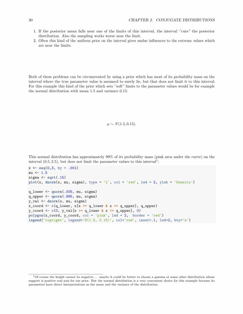
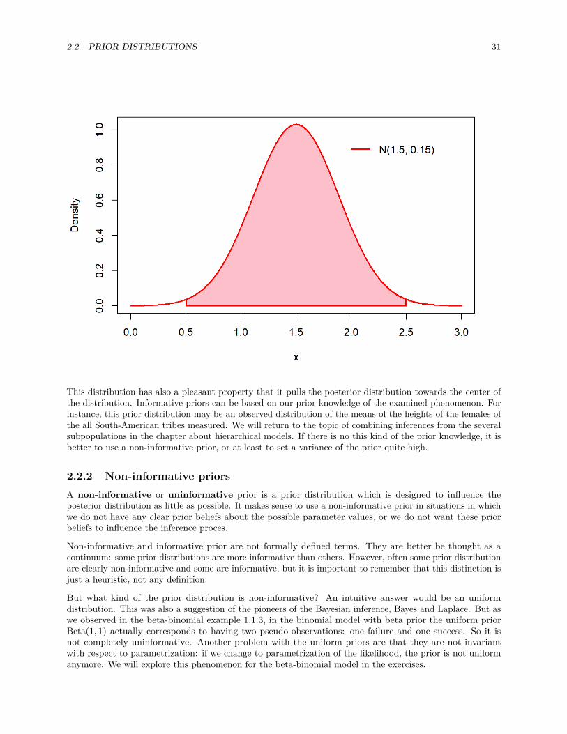
Both of these problems can be circumvented by using a prior which has most of its probability mass on theinterval where the true parameter value is assumed to surely lie, but that does not limit it to this interval.For this example this kind of the prior which sets ‘’soft” limits to the parameter values would be for examplethe normal distribution with mean 1.5 and variance 0.15:
µ ∼ N(1.5, 0.15).
This normal distribution has approximately 99% of its probability mass (pink area under the curve) on theinterval (0.5, 2.5), but does not limit the parameter values to this interval1:x <- seq(0,3, by = .001)mu <- 1.5sigma <- sqrt(.15)plot(x, dnorm(x, mu, sigma), type = 'l', col = 'red', lwd = 2, ylab = 'Density')
q_lower <- qnorm(.005, mu, sigma)q_upper <- qnorm(.995, mu, sigma)y_val <- dnorm(x, mu, sigma)x_coord <- c(q_lower, x[x >= q_lower & x <= q_upper], q_upper)y_coord <- c(0, y_val[x >= q_lower & x <= q_upper], 0)polygon(x_coord, y_coord, col = 'pink', lwd = 2, border = 'red')legend('topright', legend='N(1.5, 0.15)', col='red', inset=.1, lwd=2, bty='n')
1Of course the height cannot be negative. . . maybe it could be better to choose a gamma or some other distribution whosesupport is positive real axis for our prior. But the normal distribution is a very convenient choice for this example because itsparameters have direct interpretations as the mean and the variance of the distribution.
2.2. PRIOR DISTRIBUTIONS 31
This distribution has also a pleasant property that it pulls the posterior distribution towards the center ofthe distribution. Informative priors can be based on our prior knowledge of the examined phenomenon. Forinstance, this prior distribution may be an observed distribution of the means of the heights of the females ofthe all South-American tribes measured. We will return to the topic of combining inferences from the severalsubpopulations in the chapter about hierarchical models. If there is no this kind of the prior knowledge, it isbetter to use a non-informative prior, or at least to set a variance of the prior quite high.
2.2.2 Non-informative priorsA non-informative or uninformative prior is a prior distribution which is designed to influence theposterior distribution as little as possible. It makes sense to use a non-informative prior in situations in whichwe do not have any clear prior beliefs about the possible parameter values, or we do not want these priorbeliefs to influence the inference proces.
Non-informative and informative prior are not formally defined terms. They are better be thought as acontinuum: some prior distributions are more informative than others. However, often some prior distributionare clearly non-informative and some are informative, but it is important to remember that this distinction isjust a heuristic, not any definition.
But what kind of the prior distribution is non-informative? An intuitive answer would be an uniformdistribution. This was also a suggestion of the pioneers of the Bayesian inference, Bayes and Laplace. But aswe observed in the beta-binomial example 1.1.3, in the binomial model with beta prior the uniform priorBeta(1, 1) actually corresponds to having two pseudo-observations: one failure and one success. So it isnot completely uninformative. Another problem with the uniform priors are that they are not invariantwith respect to parametrization: if we change to parametrization of the likelihood, the prior is not uniformanymore. We will explore this phenomenon for the beta-binomial model in the exercises.

32 CHAPTER 2. CONJUGATE DISTRIBUTIONS
2.2.3 Improper priorsOften the distributions are most non-informative near the limits of their parameter space. For instance, theparameters of the beta prior Beta(α, β) can be thought as the (possibly non-integer) pseudo-observations: αrepresents pseudo-successes, and β represents pseudo-failures. With this logic the most non-informative priorwould be Beta(0, 0). But the problem with this prior is that it is not a probability distribution, because theBeta function approaches infinity when the parameters α, β → 0.
However, it turns out that we can plug this kind of the function that cannot be normalized into the properprobability distribution into the place of the prior in the Bayes’ theorem, as long the resulting posteriordistribution is a proper probability distribution. We call this kind of the priors that are not densities of anyprobability distribution as improper priors.
In the beta-binomial example we can denote the aforementioned improper prior (known as Haldane’s prior)as:
p(θ) ∝ θ−1(1− θ)−1.
It can be easily shown that the resulting posterior is proper a long as we have observes at least one successand one failure.
Improper priors are often obtained as the limits of the proper priors, and they are often used because theyare non-informative. We can demonstrate both of these properties with our height estimation example: thenoninformative prior for the average height mu would be an uniform distribution over the whole real axis:
p(µ) ∝ 1.
But of course this cannot be normalized into the probability distribution by dividing it by its integral overthe real axis, because this integral is infinite. However, the resulting posterior is a normal distribution if wehave at least one observation (assuming known variance). This improper prior can also be interpreted as anormal distribution with infinite variance.
When using improper priors, it is important to check that the resulting posterior is a proper probabilitydistribution.
Chapter 3
Summarizing the posteriordistribution
In principle, the posterior distribution contains all the information about the possible parameter values. Inpractice, we must also present the posterior distribution somehow. If the examined parameter θ is one- or twodimensional, we can simply plot the posterior distribution. Or when we use simulation to obtain values fromthe posterior, we can draw a histogram or scatterplot of the simulated values from the posterior distribution.If the parameter vector has more than two dimensions, we can plot the marginal posterior distributions ofthe parameters of interest.
However, we often also want to summarize the posterior distribution numerically. The usual summarystatistics, such as the mean, median, mode, variance, standard devation and different quantiles, that are usedto summarize probability distributions, can be used. These summary statistics are often also easier to presentand interpret than the full posterior distribution.
3.1 Credible intervalsCredible interval is a “Bayesian confidence interval”. But unlike frequentist confidence intervals, credibleintervals have a very intuitive interpretation: it turns out that we can actually say 95% credible intervalactually contains a true parameter value with 95% probability! Let’s first define as credible interval morerigorously, and then examine the most common ways to choose the credible intervals.
3.1.1 Credible interval definitionFor one-dimensional parameter Θ ∈ Ω (in this section we will also assume that the parameter is continuous,because it makes no sense to talk about the credible intervals for the discrete parameter), and confidencelevel α ∈ (0, 1), an interval Iα ⊆ Ω which contains a proportion 1− α of the probability mass of the posteriordistribution:
P (Θ ∈ Iα|Y = y) = 1− α, (3.1)
is called a credible interval1. Usually we talk about a (1− α) · 100% credible interval; for example, if theconfidence level is α = 0.05, we talk about the 95% credible interval.
1Remember that we assumed the parameter having a continuous distribution. This means that we can always choose aninterval Iα for which the condition (3.1) holds; we can choose the interval for which the probability is exactly 1 − α, so we donot have to define the credible interval of having the probability of at least 1 − α.
33
34 CHAPTER 3. SUMMARIZING THE POSTERIOR DISTRIBUTION
For the vector-valued Θ ∈ Ω ⊆ Rd, a (contiguous) region Iα ⊆ Ω containing a proportion 1 − α of theprobability mass of the posterior distribution:
P (Θ ∈ Iα|Y = y) = 1− α,
is called a credible region.
On the definition we conditioned on the observed data, but we can also talk about a credible interval beforeobserving any data. In this case a credible interval means an interval Iα containing a proportion 1− α of theprobability mass of the prior distribution:
P (Θ ∈ Iα) = 1− α.
This may actually be useful if we want to calibrate an informative prior distribution. We may for examplehave an ad hoc estimate of the region of the parameter space where the true parameter value lies with 95%certainty. Then we just have to find a prior distribution whose 95% credible interval agrees with this estimate.But usually credible intervals are examined after observing the data.
The condition (3.1) does not determine an unique (1−α) · 100% credible interval: actually there is an infinitenumber of such intervals. This means that we have to define some additional condition for choosing thecredible interval. Let’s examine two of the most common extra conditions.
3.1.2 Equal-tailed intervalAn equal-tailed interval (also called a central interval) of confidence level α is an interval
Iα = [qα/2, q1−α/2],
where qz is a z-quantile (remember that we assumed the parameter to be have a continous distribution; thismeans that the quantiles are always defined) of the posterior distribution.
For instance, 95% equal-tailed interval is an interval
I0.05 = [q0.025, q0.975],
where q0.025 and q0.975 are the quantiles of the posterior distribution. This is an interval on whose bothright and left side lies 2.5% of the probability mass of the posterior distribution; hence the name equal-tailedinterval.
If we can solve the posterior distribution in a closed form, quantiles can be obtained via the quantile functionof the posterior distribution:
P (Θ ≤ qz|Y = y) = z
FΘ|Y(qz|y) = z
qz = F−1Θ|Y(z|y),
This quantile function F−1Θ|Y is an inverse of the cumulative density function (cdf) FΘ|Y of the posterior
distribution.
Usually, when a credible interval is mentioned without specifying which type of the credible interval it is, anequal-tailed interval is meant.
However, unless the posterior distribution is unimodal and symmetric, there are point outsed of the equal-tailed credible interval having a higher posterior density than some points of the interval. If we want to choosethe credible interval so that this not happen, we can do it by using the highest posterior density criterion forchoosing it. We will examine this criterion more closely after an example of equal-tailed credible intervals.
3.1. CREDIBLE INTERVALS 35
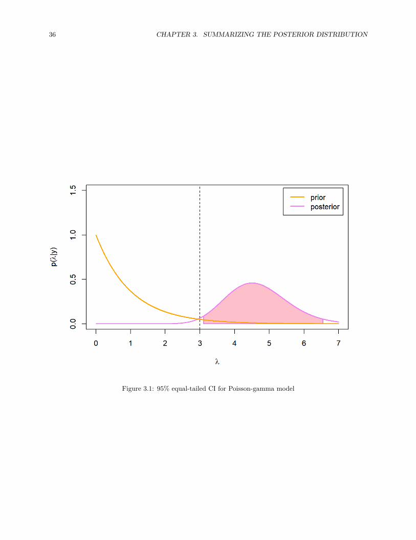
3.1.3 Example of credible intervalsLet’s revisit Example 2.1.1: we have observed a data set y = (4, 3, 11, 3, 6), and model it as a Poisson-distributed random vector Y using a gamma prior with hyperparameters α = 1, β = 1 for the parameter λ.Now we want to compute 95% confidence interval for the parameter λ.
Let’s first set up our data, hyperparameters and a confidence level:y <- c(4, 3, 11, 3, 6)n <- length(y)alpha <- 1beta <- 1
alpha_conf <- 0.05
A posterior distribution for the parameter λ is Gamma(ny + α, n+ β). Let’s set up also the parameters ofthe posterior distribution:alpha_1 <- sum(y) + alphabeta_1 <- n + beta
Now we can compute 0.025- and 0.975-quantiles using the quantile function F−1Λ|Y of the posterior distribution:
q0.025 = F−1Λ|Y(0.025|y)
q0.975 = F−1Λ|Y(0.975|y).
Luckily R contains a quantile function of the gamma distribution, so we get the 95% credible interval simplyas:q_lower <- qgamma(alpha_conf / 2, alpha_1, beta_1)q_upper <- qgamma(1 - alpha_conf / 2, alpha_1, beta_1)c(q_lower, q_upper)
## [1] 3.100966 6.547264
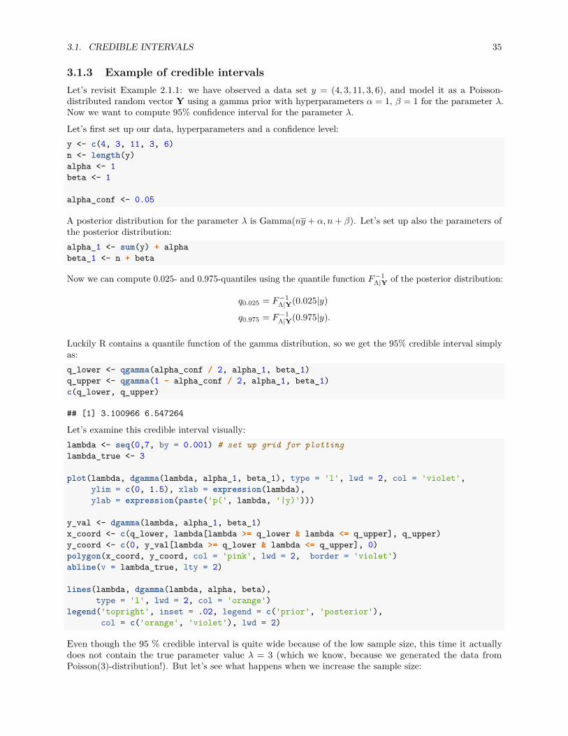
Let’s examine this credible interval visually:lambda <- seq(0,7, by = 0.001) # set up grid for plottinglambda_true <- 3
plot(lambda, dgamma(lambda, alpha_1, beta_1), type = 'l', lwd = 2, col = 'violet',ylim = c(0, 1.5), xlab = expression(lambda),ylab = expression(paste('p(', lambda, '|y)')))
y_val <- dgamma(lambda, alpha_1, beta_1)x_coord <- c(q_lower, lambda[lambda >= q_lower & lambda <= q_upper], q_upper)y_coord <- c(0, y_val[lambda >= q_lower & lambda <= q_upper], 0)polygon(x_coord, y_coord, col = 'pink', lwd = 2, border = 'violet')abline(v = lambda_true, lty = 2)
lines(lambda, dgamma(lambda, alpha, beta),type = 'l', lwd = 2, col = 'orange')
legend('topright', inset = .02, legend = c('prior', 'posterior'),col = c('orange', 'violet'), lwd = 2)
Even though the 95 % credible interval is quite wide because of the low sample size, this time it actuallydoes not contain the true parameter value λ = 3 (which we know, because we generated the data fromPoisson(3)-distribution!). But let’s see what happens when we increase the sample size:
36 CHAPTER 3. SUMMARIZING THE POSTERIOR DISTRIBUTION
Figure 3.1: 95% equal-tailed CI for Poisson-gamma model
3.1. CREDIBLE INTERVALS 37
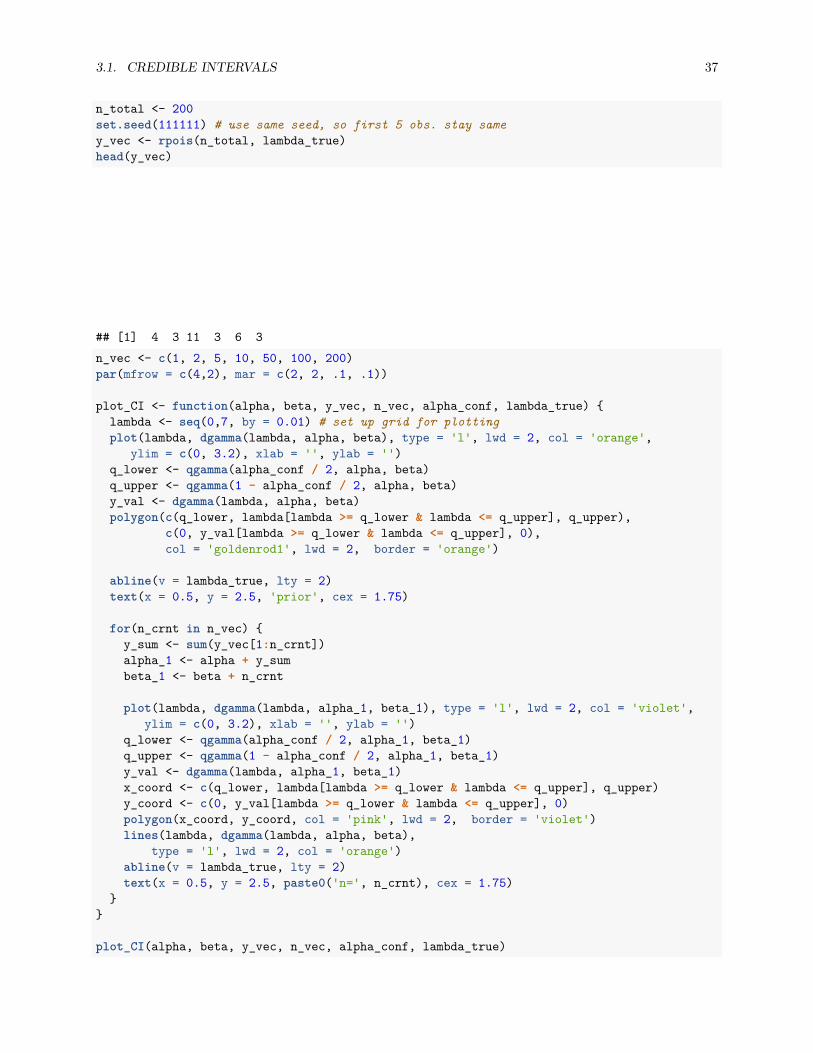
n_total <- 200set.seed(111111) # use same seed, so first 5 obs. stay samey_vec <- rpois(n_total, lambda_true)head(y_vec)
## [1] 4 3 11 3 6 3n_vec <- c(1, 2, 5, 10, 50, 100, 200)par(mfrow = c(4,2), mar = c(2, 2, .1, .1))
plot_CI <- function(alpha, beta, y_vec, n_vec, alpha_conf, lambda_true) lambda <- seq(0,7, by = 0.01) # set up grid for plottingplot(lambda, dgamma(lambda, alpha, beta), type = 'l', lwd = 2, col = 'orange',
ylim = c(0, 3.2), xlab = '', ylab = '')q_lower <- qgamma(alpha_conf / 2, alpha, beta)q_upper <- qgamma(1 - alpha_conf / 2, alpha, beta)y_val <- dgamma(lambda, alpha, beta)polygon(c(q_lower, lambda[lambda >= q_lower & lambda <= q_upper], q_upper),
c(0, y_val[lambda >= q_lower & lambda <= q_upper], 0),col = 'goldenrod1', lwd = 2, border = 'orange')
abline(v = lambda_true, lty = 2)text(x = 0.5, y = 2.5, 'prior', cex = 1.75)
for(n_crnt in n_vec) y_sum <- sum(y_vec[1:n_crnt])alpha_1 <- alpha + y_sumbeta_1 <- beta + n_crnt
plot(lambda, dgamma(lambda, alpha_1, beta_1), type = 'l', lwd = 2, col = 'violet',ylim = c(0, 3.2), xlab = '', ylab = '')
q_lower <- qgamma(alpha_conf / 2, alpha_1, beta_1)q_upper <- qgamma(1 - alpha_conf / 2, alpha_1, beta_1)y_val <- dgamma(lambda, alpha_1, beta_1)x_coord <- c(q_lower, lambda[lambda >= q_lower & lambda <= q_upper], q_upper)y_coord <- c(0, y_val[lambda >= q_lower & lambda <= q_upper], 0)polygon(x_coord, y_coord, col = 'pink', lwd = 2, border = 'violet')lines(lambda, dgamma(lambda, alpha, beta),
type = 'l', lwd = 2, col = 'orange')abline(v = lambda_true, lty = 2)text(x = 0.5, y = 2.5, paste0('n=', n_crnt), cex = 1.75)
plot_CI(alpha, beta, y_vec, n_vec, alpha_conf, lambda_true)
38 CHAPTER 3. SUMMARIZING THE POSTERIOR DISTRIBUTION
When we observe more data, the credible interval get narrower. This reflects our growing certainty about therange where the true parameter value lies. Turns out that this time the credible interval contains the trueparameter value with all the other tested sample sizes expect n = 5.
But unlike the frequentist confidence interval, the credible interval does not depend only on the data: theprior distribution also influences the credible intervals. That orange area in the first of the figures is a credibleinterval that is computed using the prior distribution. It describes our belief where 95% of the probabilitymass of the distribution should lie before we observe any data.
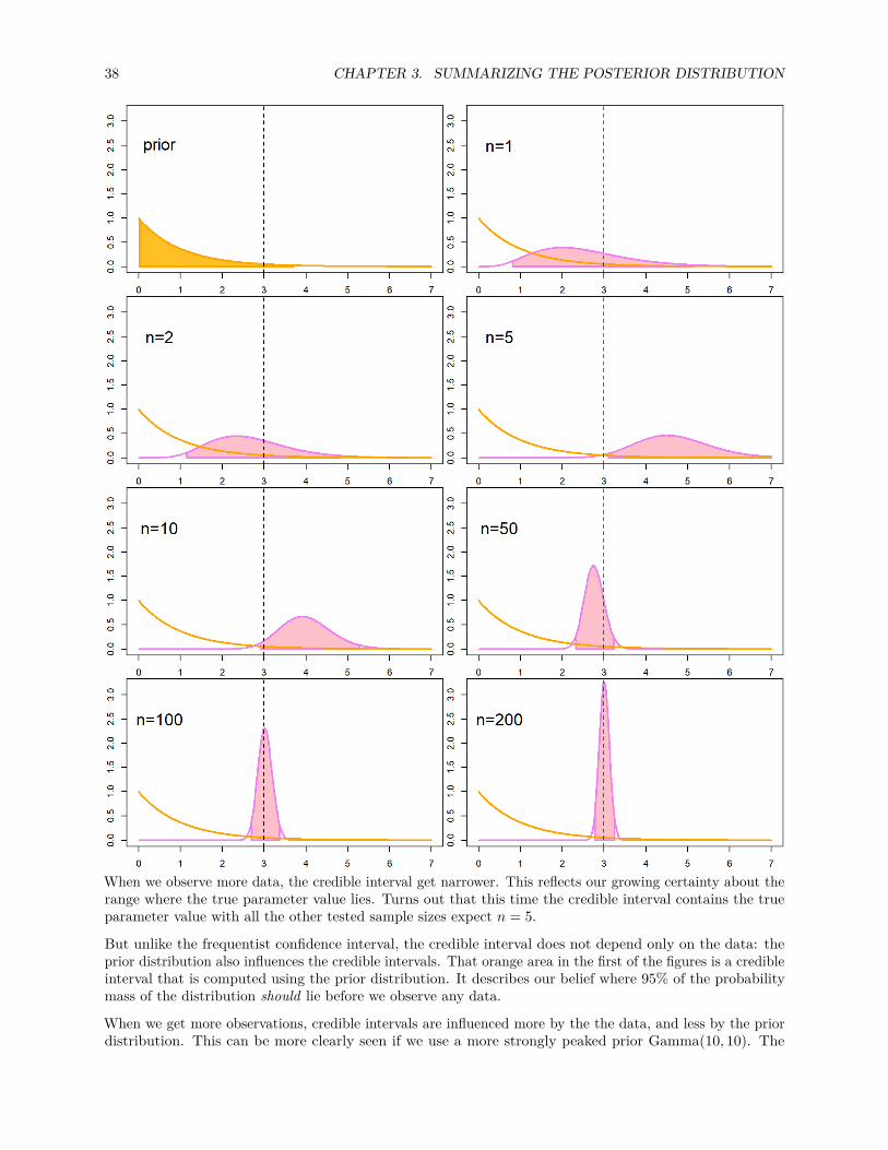
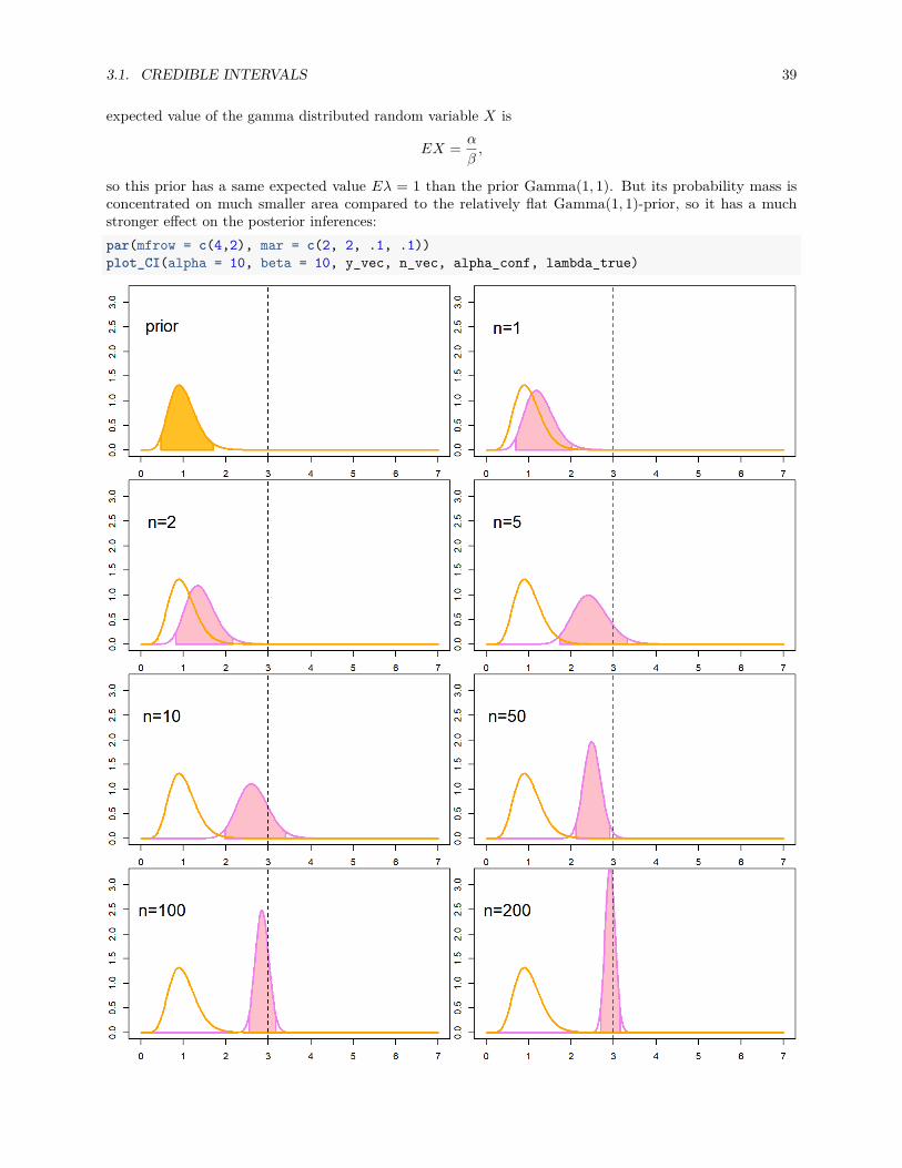
When we get more observations, credible intervals are influenced more by the the data, and less by the priordistribution. This can be more clearly seen if we use a more strongly peaked prior Gamma(10, 10). The
3.1. CREDIBLE INTERVALS 39
expected value of the gamma distributed random variable X is
EX = α
β,
so this prior has a same expected value Eλ = 1 than the prior Gamma(1, 1). But its probability mass isconcentrated on much smaller area compared to the relatively flat Gamma(1, 1)-prior, so it has a muchstronger effect on the posterior inferences:par(mfrow = c(4,2), mar = c(2, 2, .1, .1))plot_CI(alpha = 10, beta = 10, y_vec, n_vec, alpha_conf, lambda_true)
40 CHAPTER 3. SUMMARIZING THE POSTERIOR DISTRIBUTION
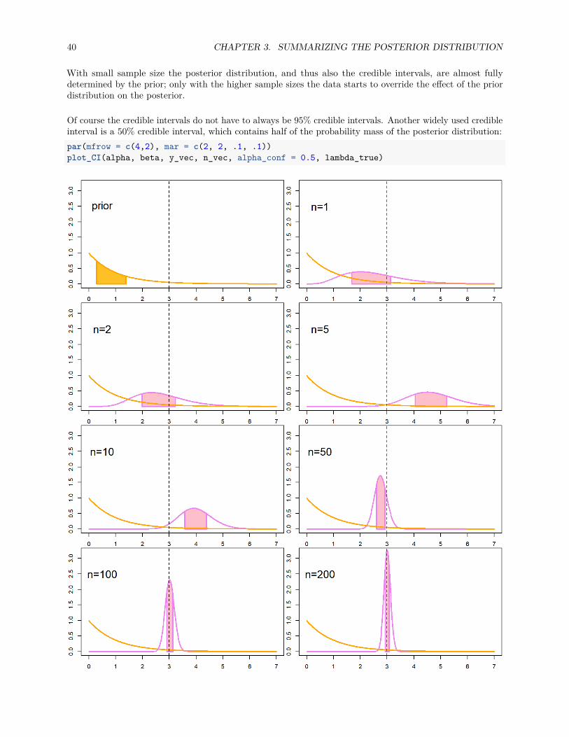
With small sample size the posterior distribution, and thus also the credible intervals, are almost fullydetermined by the prior; only with the higher sample sizes the data starts to override the effect of the priordistribution on the posterior.
Of course the credible intervals do not have to always be 95% credible intervals. Another widely used credibleinterval is a 50% credible interval, which contains half of the probability mass of the posterior distribution:par(mfrow = c(4,2), mar = c(2, 2, .1, .1))plot_CI(alpha, beta, y_vec, n_vec, alpha_conf = 0.5, lambda_true)
3.1. CREDIBLE INTERVALS 41
3.1.4 Highest posterior density region
A highest posterior density (HPD) region of confidence level α is a (1−α)-confidence region Iα for whichholds that the posterior density for every point in this set is higher than the posterior density for any pointoutside of this set:
fΘ|Y(θ|y) ≥ fΘ|Y(θ′|y)
for all θ ∈ Iα, θ′ /∈ Iα. This means that a (1 − α)-highest density posterior region is a smallest possible(1− α)-credible region.
An observant reader may notice that the HPD region is not necessarily an interval (or a contiguous region in ahigher-dimensional case): if the posterior distribution is multimodal, the HPD region of this distribution maybe an union of distinct intervals (or distinct contiguous regions in a higher-dimensional case). This meansthat HPD regions are not necessarily always strictly credible intervals or regions according to Definition (3.1).However, in Bayesian statistics we often talk simply about HPD intervals, even though may not always beintervals.
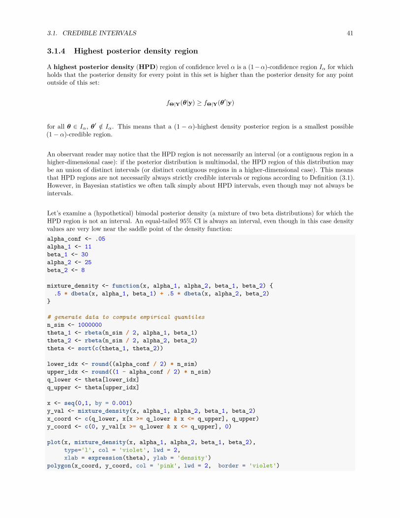
Let’s examine a (hypothetical) bimodal posterior density (a mixture of two beta distributions) for which theHPD region is not an interval. An equal-tailed 95% CI is always an interval, even though in this case densityvalues are very low near the saddle point of the density function:alpha_conf <- .05alpha_1 <- 11beta_1 <- 30alpha_2 <- 25beta_2 <- 8
mixture_density <- function(x, alpha_1, alpha_2, beta_1, beta_2) .5 * dbeta(x, alpha_1, beta_1) + .5 * dbeta(x, alpha_2, beta_2)
# generate data to compute empirical quantilesn_sim <- 1000000theta_1 <- rbeta(n_sim / 2, alpha_1, beta_1)theta_2 <- rbeta(n_sim / 2, alpha_2, beta_2)theta <- sort(c(theta_1, theta_2))
lower_idx <- round((alpha_conf / 2) * n_sim)upper_idx <- round((1 - alpha_conf / 2) * n_sim)q_lower <- theta[lower_idx]q_upper <- theta[upper_idx]
x <- seq(0,1, by = 0.001)y_val <- mixture_density(x, alpha_1, alpha_2, beta_1, beta_2)x_coord <- c(q_lower, x[x >= q_lower & x <= q_upper], q_upper)y_coord <- c(0, y_val[x >= q_lower & x <= q_upper], 0)
plot(x, mixture_density(x, alpha_1, alpha_2, beta_1, beta_2),type='l', col = 'violet', lwd = 2,xlab = expression(theta), ylab = 'density')
polygon(x_coord, y_coord, col = 'pink', lwd = 2, border = 'violet')
42 CHAPTER 3. SUMMARIZING THE POSTERIOR DISTRIBUTION
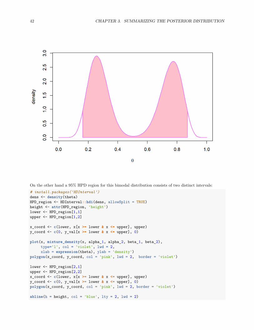
On the other hand a 95% HPD region for this bimodal distribution consists of two distinct intervals:# install.packages('HDInterval')dens <- density(theta)HPD_region <- HDInterval::hdi(dens, allowSplit = TRUE)height <- attr(HPD_region, 'height')lower <- HPD_region[1,1]upper <- HPD_region[1,2]
x_coord <- c(lower, x[x >= lower & x <= upper], upper)y_coord <- c(0, y_val[x >= lower & x <= upper], 0)
plot(x, mixture_density(x, alpha_1, alpha_2, beta_1, beta_2),type='l', col = 'violet', lwd = 2,xlab = expression(theta), ylab = 'density')
polygon(x_coord, y_coord, col = 'pink', lwd = 2, border = 'violet')
lower <- HPD_region[2,1]upper <- HPD_region[2,2]x_coord <- c(lower, x[x >= lower & x <= upper], upper)y_coord <- c(0, y_val[x >= lower & x <= upper], 0)polygon(x_coord, y_coord, col = 'pink', lwd = 2, border = 'violet')
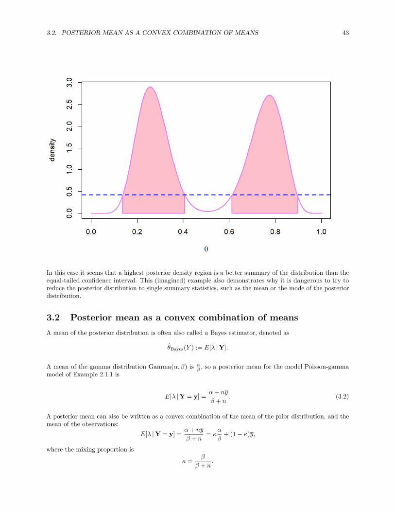
abline(h = height, col = 'blue', lty = 2, lwd = 2)
3.2. POSTERIOR MEAN AS A CONVEX COMBINATION OF MEANS 43
In this case it seems that a highest posterior density region is a better summary of the distribution than theequal-tailed confidence interval. This (imagined) example also demonstrates why it is dangerous to try toreduce the posterior distribution to single summary statistics, such as the mean or the mode of the posteriordistribution.
3.2 Posterior mean as a convex combination of meansA mean of the posterior distribution is often also called a Bayes estimator, denoted as
θBayes(Y ) := E[λ |Y].
A mean of the gamma distribution Gamma(α, β) is αβ , so a posterior mean for the model Poisson-gamma
model of Example 2.1.1 is
E[λ |Y = y] = α+ ny
β + n. (3.2)
A posterior mean can also be written as a convex combination of the mean of the prior distribution, and themean of the observations:
E[λ |Y = y] = α+ ny
β + n= κ
α
β+ (1− κ)y,
where the mixing proportion is
κ = β
β + n.
44 CHAPTER 3. SUMMARIZING THE POSTERIOR DISTRIBUTION
The higher the sample size, the higher is the contribution of the data to the posterior mean (compared to thecontribution of the prior mean). And at the limit when n→∞, κ→ 0. This means that for this model theposterior mean is asymptotically equivalent to the maximum likelihood estimator, which for this model isjust the mean of the observations:
θMLE(Y) = Y .
The formula for the posterior mean of the Poisson-gamma model given in Equation (3.2) also gives us a hintwhy increasing the rate parameter β of the prior gamma distribution increased the effect of the prior of theposterior distribution: The location parameter α is added to the sum of the observations, and β is added tothe sample size. So the prior could be interpreted as “pseudo-observations” that are added to the actualobservations: parameter α could be interpreted as the “pseudo-events”, and β as the “pseudo-sample size”(although they are not necessarily integers). So using prior α = 15, β = 10 could be interpreted as having aprior data set of 10 observations, and having total 15 events in this data set.
Chapter 4
Approximate inference
In the preceding chapters we have examined conjugate models for which it is possible to solve the marginallikelihood, and thus also the posterior and the posterior predictive distributions in a closed form. However,in more realistic scenarios in which more complex models are required, the marginal likelihood is usuallyintractable, and because of this the posterior cannot be solved analytically.
This means that usually we have to approximate the posterior distribution p(θ|y) somehow, and then usethis approximation to compute the quantities of interest, such as posterior mean or credible intervals.
In general, there are two ways to approximate the posterior distribution:
1. Simulation: generate a random sample from the posterior distribution, and use its empirical distributionfunction as an approximation of the posterior.
2. Distributional approximation: approximate the posterior directly by some simpler parametric distribu-tion, such as the normal distribution.
A simple form of the distributional approxmation is a normal approximation, where the central limit theoremis invoked to justify the use of normal distribution to approximate the posterior distribution. This is analogousto the normal approximation used in frequentist statistics to approximate the distribution of the estimator ofthe parameter of interest with high sample sizes. More generally, approximating the posterior density bysome tractable density q(θ) is called variational inference.
However, on the rest of this chapter we will focus to the approximating the posterior distribution by generatinga random sample from it.
4.1 Simulation methodsThe first step is to generate a random sample θ1, . . . ,θS from a posterior distribution p(θ|y). If the posteriordistribution is a known distribution, whose simulation method has been implemented in R or Python, thenthis is of course easy. Of course, in this case you do not need the sample the posterior to distribution toapproximate it, because you already know the exact posterior distribution. However, the simulating the maystill be the easiest way to evaluate some integrals over the posterior distributions, such as the probability ofsome set. We will return to this later in this section.
But let’s consider the more interesting case, where the posterior distribution cannot be solved in a closed form.Now you may be wondering how on earth is it possible to generate sample from the unknown distribution?Turns out that this is actually super easy: even though the normalizing constant p(y) is unknown, we canutilize the same trick that we used to compute the posterior analytically for the conjugate models. Instead ofthe posterior density, it is sufficient to generate a random sample from an unnormalized posterior density,that is, any function θ → q(θ; y), which is proportional to the posterior density:
p(θ|y) ∝ q(θ; y).
45
46 CHAPTER 4. APPROXIMATE INFERENCE
In particular, we can utilize the unnormalized version of the Bayes’ theorem:
p(θ|y) ∝ p(θ)p(y|θ),
and simulate the posterior by generating a random sample from the unnormalized posterior distributionq(θ; y) ∝ p(θ)p(y|θ).
Now the only problem is how to generate this random sample? This can be done for example by rejectionsampling or importance sampling for the simple models. On this course we will not concentrate onthese sampling methods. For those more interested on the sampling methods, there is a course calledComputational statistics, which is dedicated solely on the computational aspects of Bayesian inference.It will be possible to do the course as self-study next spring, and it will be lectured with a high probabilitynext autumn.
Fortunately, there are nowadays automated probabilistic programming tools that to these simulationsautomatically for us, so that we do not have to write a sampler manually each time we want to simulatefrom a new posterior distribution. So our plan is to demonstrate simulation from the posterior distributionmanually with a simple example, and after this to introduce these automated tools that make a life of thestatistician easier.
4.1.1 Grid approximationFor our example we will use a straightforward simulation recipe called grid approximation or directdiscrete approximation:
1. Create an even-spaced grid g1 = a + i/2, . . . , gm = b − i/2, where a is the lower, and b is the upperlimit of the interval on which we want to evaluate the posterior, i is the increment of the grid, and m isthe number of grid points.
2. Evaluate values of the unnormalized posterior density in the grid points q(g1; y), . . . , q(gm; y), andnormalized them to obtain the estimated values of the posterior distribution at the grid points:
p1 := q(g1; y)∑mi=1 q(gi; y) , . . . , pm := q(gm; y)∑m
i=1 q(gi; y)
3. For every s = 1, . . . , S:• Generate λs from a categorical distribution with outcomes g1, . . . , gm which have the probabilitiesp1, . . . , pn
• Add jitter which is uniformly distributed around zero, and whose interval length is equal to thegrid spacing, to the generated values: λs = λs +X, where X ∼ U(−i/2, i/2) (to push generatedvalues out of the grid points).
You may have observed that this basically amounts to performing a numerical integration by sampling. Gridapproximation also has the downsides of numerical integration: we can only simulate from the finite interval,and if we keep the grid spacing constant, the size of the grid grows exponentially w.r.t. dimension of theparameter. However, this crude method will do for our introductory example.
4.1.2 Example: grid approximationLet’s demonstrate a simulation from the posterior distribution with the Poisson-gamma conjugate model ofExample 2.1.1. Of course we know that the true posterior distribution for this model is
Gamma(α+ ny, β + n),
and thus we wouldn’t have to simulate at all to find out the posterior of this model. However, the point ofdoing simulation first with a known distribution is to verify that our simulation method works by confirmingthat the simulated posterior density is very close to the analytically solved posterior density.
Let’s start by setting the same parameter values and generating the same observations used in Example 2.1.1:
4.1. SIMULATION METHODS 47
lambda_true <- 3alpha <- beta <- 1n <- 5set.seed(111111)y <- rpois(n, lambda_true)y
## [1] 4 3 11 3 6
The unormalized posterior for this model can be written (cf. Equation (2.1)) as:
q(λ; y) = λ∑n
i=1yi+α−1e−(n+β)λ
Let’s define this as a function:q <- function(lambda, y, n, alpha, beta)
lambda^(alpha + sum(y) - 1) * exp(-(n + beta) * lambda)
The parameter space Ω = (0,∞) is a whole positive real axis. But this crude simulation method we usehas a limitation that an interval on which we simulate the posterior distribution must be finite. How dowe then choose this interval? In a real scenario, we would compute some initial point estimates such asmaximum likelihood estimates for the mean and the variance of the parameter, and then use these to choosean interval which should contain almost all of the probability mass of the posterior distribution. However, inthis introductory example we have already seen the true posterior, so we can be sure that for example theinterval (0, 20) contains almost all of the probability mass of the distribution. So let’s use set a grid on theinterval (0, 20) by an increment i = 0.01, evaluate the unnormalized density at the points of this grid, andnormalize the values by dividing them by the sum of all values:lower_lim <- 0upper_lim <- 20i <- 0.01grid <- seq(lower_lim + i/2, upper_lim - i/2, by = i)
n_sim <- 1e4n_grid <- length(grid)grid_values <- q(grid, y, n, alpha, beta)normalized_values <- grid_values / sum(grid_values)
Now the probabilities p1, . . . , pm sum to one, and thus define a proper categorical probability distribution(with grid points g1, . . . , gm being the values into which these probabilities correspond to). Let’s generate thesample λ1, . . . , λS from this distribution, and then add some uniform jitter to them:idx_sim <- sample(1:n_grid, n_sim, prob = normalized_values, replace = TRUE)lambda_sim <- grid[idx_sim]
X <- runif(n_sim, -i/2, i/2)lambda_sim <- lambda_sim + X
Now we should have simulated a sample from the posterior distribution. Let’s draw a histogram of oursample, and overlay it with the analytically solved posterior distribution to see if they match:hist(lambda_sim, col = 'violet', breaks = seq(0,10, by =.25), probability = TRUE,
main = '', xlab = expression(lambda), xlim = c(0,10))lines(grid, dgamma(grid, alpha + sum(y), beta + n), type = 'l', col = 'green', lwd=3 )legend('topright', legend = 'True posterior', bty = 'n',
col = 'green', lwd = 2, inset = .02)
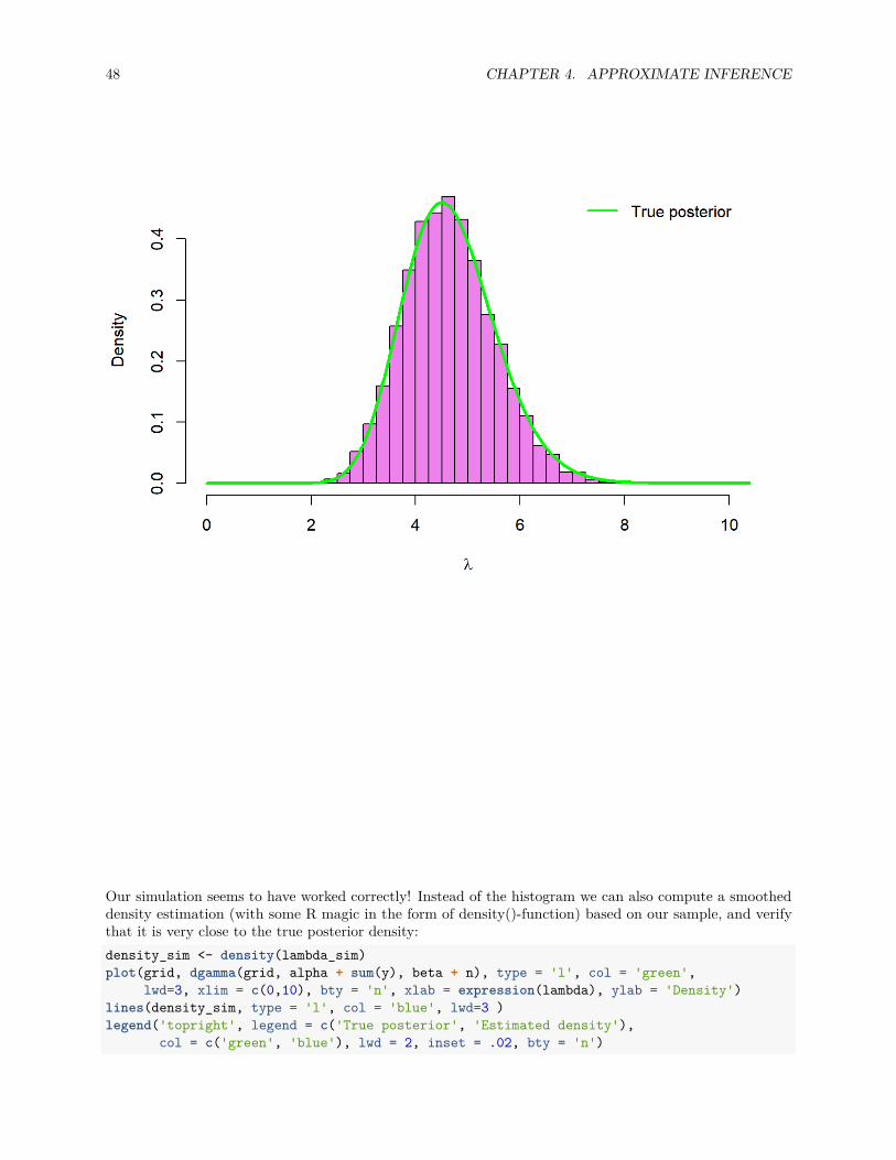
48 CHAPTER 4. APPROXIMATE INFERENCE
Our simulation seems to have worked correctly! Instead of the histogram we can also compute a smootheddensity estimation (with some R magic in the form of density()-function) based on our sample, and verifythat it is very close to the true posterior density:density_sim <- density(lambda_sim)plot(grid, dgamma(grid, alpha + sum(y), beta + n), type = 'l', col = 'green',
lwd=3, xlim = c(0,10), bty = 'n', xlab = expression(lambda), ylab = 'Density')lines(density_sim, type = 'l', col = 'blue', lwd=3 )legend('topright', legend = c('True posterior', 'Estimated density'),
col = c('green', 'blue'), lwd = 2, inset = .02, bty = 'n')
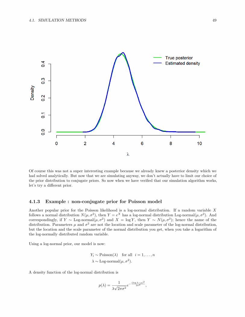
4.1. SIMULATION METHODS 49
Of course this was not a super interesting example because we already knew a posterior density which wehad solved analytically. But now that we are simulating anyway, we don’t actually have to limit our choice ofthe prior distribution to conjugate priors. So now when we have verified that our simulation algorithm works,let’s try a different prior.
4.1.3 Example : non-conjugate prior for Poisson model
Another popular prior for the Poisson likelihood is a log-normal distribution. If a random variable Xfollows a normal distribution N(µ, σ2), then Y = eX has a log-normal distribution Log-normal(µ, σ2). Andcorrespondingly, if Y ∼ Log-normal(µ, σ2) and X = log Y , then Y ∼ N(µ, σ2); hence the name of thedistribution. Parameters µ and σ2 are not the location and scale parameter of the log-normal distribution,but the location and the scale parameter of the normal distribution you get, when you take a logarithm ofthe log-normally distributed random variable.
Using a log-normal prior, our model is now:
Yi ∼ Poisson(λ) for all i = 1, . . . , nλ ∼ Log-normal(µ, σ2).
A density function of the log-normal distribution is
p(λ) = 1λ√
2πσ2e−
(logλ−µ)2
2σ2 ,
50 CHAPTER 4. APPROXIMATE INFERENCE
and thus we can write the unnormalized posterior density as
p(λ|y) ∝ p(λ)p(y|λ)
∝ λ−1e(logλ−µ)2
2σ2 λ∑n
i=1yie−nλ
∝ λ∑n
i=1yi−1e−nλ−
(logλ−µ)2
2σ2 .
This cannot be normalized into any known probability distribution: the normalizing constant
p(y) =∫p(λ)p(y|λ)dλ
is intractable! But this is not a problem, because we know how to simulate from an unormalized posteriordistribution. Let’s first define a function1 for the unnormalized posterior:q <- function(lambda, y, n, mu, sigma_squared)
lambda^(sum(y) - 1) * exp(-n * lambda - (log(lambda) - mu)^2 / (2 * sigma_squared))
Let’s also set parameters µ = 0, σ2 = 1 of the prior:mu <- 0sigma_squared <- 1
Now we are ready to use our simulation recipe again, and visualize the results:grid_values <- q(grid, y, n, mu, sigma_squared)normalized_values <- grid_values / sum(grid_values)idx_sim <- sample(1:n_grid, n_sim, prob = normalized_values, replace = TRUE)lambda_sim2 <- grid[idx_sim] + runif(n_sim, -i/2, i/2)
hist(lambda_sim2, col = 'violet', breaks = seq(0,10, by =.25), probability = TRUE,main = '', xlab = expression(lambda), xlim = c(0,10), ylim = c(0, 0.5))
lines(grid, dgamma(grid, alpha + sum(y), beta + n), type='l', col='green', lwd=3)legend('topright', legend = paste0('Gamma(', sum(y) + alpha, ',', n + beta, ')'),
col = 'green', lwd = 2, inset = .02, bty = 'n')
1Normally we would compute with the logarithms, which means using values of the function log q(λ; y) instead of q(λ; y),and exponentiate as late as possible to avoid over- and underflows and other numerical problems. However, let’s not complicatethings unnecessarily in this introductory example.
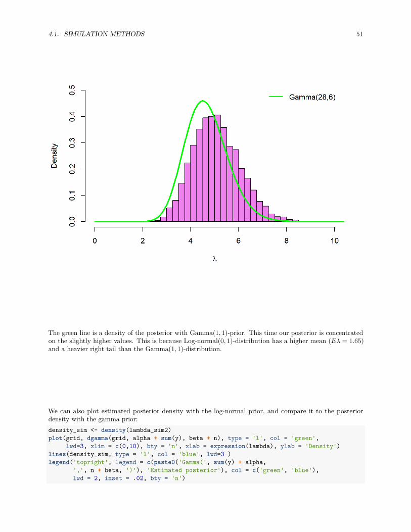
4.1. SIMULATION METHODS 51
The green line is a density of the posterior with Gamma(1, 1)-prior. This time our posterior is concentratedon the slightly higher values. This is because Log-normal(0, 1)-distribution has a higher mean (Eλ = 1.65)and a heavier right tail than the Gamma(1, 1)-distribution.
We can also plot estimated posterior density with the log-normal prior, and compare it to the posteriordensity with the gamma prior:density_sim <- density(lambda_sim2)plot(grid, dgamma(grid, alpha + sum(y), beta + n), type = 'l', col = 'green',
lwd=3, xlim = c(0,10), bty = 'n', xlab = expression(lambda), ylab = 'Density')lines(density_sim, type = 'l', col = 'blue', lwd=3 )legend('topright', legend = c(paste0('Gamma(', sum(y) + alpha,
',', n + beta, ')'), 'Estimated posterior'), col = c('green', 'blue'),lwd = 2, inset = .02, bty = 'n')
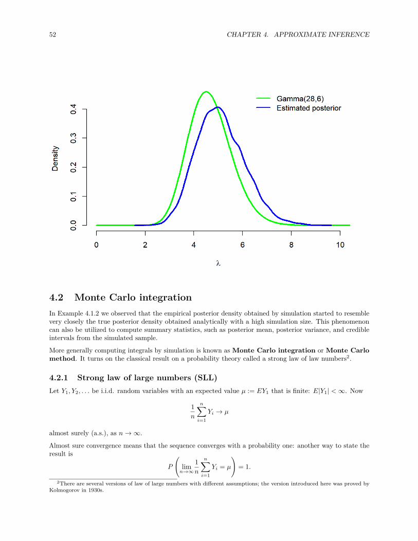
52 CHAPTER 4. APPROXIMATE INFERENCE
4.2 Monte Carlo integrationIn Example 4.1.2 we observed that the empirical posterior density obtained by simulation started to resemblevery closely the true posterior density obtained analytically with a high simulation size. This phenomenoncan also be utilized to compute summary statistics, such as posterior mean, posterior variance, and credibleintervals from the simulated sample.
More generally computing integrals by simulation is known as Monte Carlo integration or Monte Carlomethod. It turns on the classical result on a probability theory called a strong law of law numbers2.
4.2.1 Strong law of large numbers (SLL)Let Y1, Y2, . . . be i.i.d. random variables with an expected value µ := EY1 that is finite: E|Y1| <∞. Now
1n
n∑i=1
Yi → µ
almost surely (a.s.), as n→∞.
Almost sure convergence means that the sequence converges with a probability one: another way to state theresult is
P
(limn→∞
1n
n∑i=1
Yi = µ
)= 1.
2There are several versions of law of large numbers with different assumptions; the version introduced here was proved byKolmogorov in 1930s.
4.2. MONTE CARLO INTEGRATION 53
4.2.2 Example of SLL : coinflipsThe strong law of law number simply states that the sample mean of i.i.d. random variables converges to anexpected value of the distribution with probability one. We intuitively use this result all the time, but thestrong law of large numbers states it formally.
Denote by Y1, Y2, . . . a series of coinflips, where Y1 = 1 means heads and Y1 = 0 means tails. Assuming a faircoin, P (Y1 = 1) = 1/2, and thus µ = EY1 = 1/2. By a strong law of large numbers the proportion of headsconverges to the probability of heads:
1n
n∑i=1
Yia.s.→ 1
2
with probability one. Although there exists an infinite number of sequences which do not converge to 1/2,such as a sequence of only heads (1, 1, . . . ), the probability of the set of these sequences is zero.
4.2.3 Example of Monte carlo integrationLet’s revisit Example 4.1.1. Because our simulated values λ1, . . . λS are an i.i.d. sample of the posteriordistribution, which has a finite expected value, by the strong law of large numbers the posterior meanconverges almost surely to this expected value:
1S
S∑i=1
λia.s.→ E[Λ |Y = y].
This means that we can approximate the posterior expectation with the posterior mean:
E[Λ |Y = y] ≈ 1S
S∑i=1
λi.
Because we know the posterior expectation
E[Λ |Y = y] = α1
β1=∑ni=1 Yi + α
n+ β
for this example, we can verify that the posterior mean is very close to the true expected value:alpha_1 <- alpha + sum(y)beta_1 <- beta + nalpha_1 / beta_1
## [1] 4.666667mean(lambda_sim)
## [1] 4.648235
The second moment Eλ2 of the posterior distribution also exists, so we can invoke again the strong law oflarge numbers for the sequence of random variables Λ2
1,Λ22, . . . to approximate the posterior variance:
Var[Λ |Y = y] = E[Λ2 |Y = y]− E[Λ |Y = y]
≈ 1S
S∑i=1
λ2i −
1S
S∑i=1
λi
= 1S − 1
S∑i=1
(λi − λ)2.
Again the empirical variance is very close to the true variance of the posterior distribution:
54 CHAPTER 4. APPROXIMATE INFERENCE
alpha_1 / beta_1^2
## [1] 0.7777778var(lambda_sim)
## [1] 0.7517682
We can also use SLL for the sequence of transformations I(a,b)(Λ1), I(a,b)(Λ2), . . . of the parameter Λ, whereI(a,b) is an indicator function:
I(a,b)(x) =
1 if x ∈ (a, b),0 otherwise.
This means that we can approximate the posterior probabilities by the empirical proportions:
P (a < Λ < b |Y = y) = E[I(a,b)(Λ) |Y = y]
≈ 1S
S∑i=1
I(a,b)(λi)
= 1S
#a < λi < b.
Here # marks the number of elements of the set. Let’s demonstrate this by approximating the posteriorprobabilities P (Λ > 3 |Y = y):pgamma(3, alpha_1, beta_1, lower.tail = FALSE)
## [1] 0.9826824mean(lambda_sim > 3)
## [1] 0.9811
and P (4 < Λ < 6 |Y = y):pgamma(6, alpha_1, beta_1) - pgamma(4, alpha_1, beta_1)
## [1] 0.694159mean(lambda_sim > 4 & lambda_sim < 6)
## [1] 0.6984
Because the empirical distribution function can be used to approximate the cumulative density function FΛ|Yof the posterior distribution, we can also use the empirical quantiles to estimate the quantiles of the posteriordistribution, and thus to approximate equal-tailed credible intervals:alpha_conf <- 0.05qgamma(alpha_conf / 2, alpha_1, beta_1) # 0.025 - quantile
## [1] 3.100966quantile(lambda_sim, alpha_conf / 2)
## 2.5%## 3.081615qgamma(1 - alpha_conf / 2, alpha_1, beta_1) # 0.975 - quantiles
## [1] 6.547264

4.3. MONTE CARLO MARKOV CHAIN (MCMC) METHODS 55
quantile(lambda_sim, 1 - alpha_conf / 2)
## 97.5%## 6.484451
Normally strong law of law numbers is not mentioned explicitly when the empirical quantities are used toapproximate expected values, but anyway it is a theoretical result behind these approximations. Also thefiniteness of the expected value of the posterior is rarely checked explicitly. However, in the exercises we willhave an example of the distribution for which the expected value is infinite.
4.3 Monte Carlo markov chain (MCMC) methodsOur simple grid approximation method worked smoothly, but what would happen if the dimension of theparameter were higher? In our example we set a grid on the interval (0, 10) with a grid increment i = 0.01,so the grid had 1000 points. If the parameter were two-dimensional, the grid with the same increment overthe two-dimensional interval (0, 10)× (0, 10) would have million points. And to approximate 3-dimensionalparameter with the same grid increment we would need milliard grid points!
Hence, grid approximation quickly becomes infeasible as the dimension of the parameter grows. Rejection andimportance sampling have similar problems. This is why for the more complex models sampling is usuallydone by using Monte Carlo markov chain (MCMC) methods. They are based by iteratively samplingfrom a Markov chain whose stationary distribution is the target distribution, which in the case of Bayesiancomputation is most often the posterior distribution p(θ|y).
4.3.1 Markov chainA discrete time Markov chain is a sequence of random variables X1,X2, . . ., which has a Markov property:
P (Xi+1 = xi+1 |Xi = xi, . . . , X0 = x0) = P (Xi+1 = xi+1 |Xi = xi)
for all i = 1, 2, . . .. This means that any given time the future state Xi+1 of the state depends only on thepresent state Xi of the chain, and not on the rest of the history.
A state space S of the Markov chain is the set of all possible values for these random variables Xi.
4.3.2 MCMC samplingSimple simulation methods, such as rejection sampling, importance sampling, and grid approximation, whichwe just demonstrated, generate an i.i.d. sample from the target distribution. However, the components of thesample θ1, . . . ,θS generated by the Monte Carlo markov chain methods has a very high autocorrelation: thismeans that next value θi+1 is likely to be somewhere near the current value θi of the chain. But how doesthis even work? The trick is that because we generate a large sample, and then use the whole sample toapproximate our posterior distribution, the autocorrelation of the single values does not matter.
We already mentioned that the Markov chains used in MCMC methods are designed so that their stationarydistribution is the target posterior distribution. But what does the stationary distribution mean? It issimply a distribution π(x) with a following property: if you start the chain from the stattionary distributionso that P (X0 = k) = π(k) for all k ∈ S, then also P (Xi = k) = π(k) for all i = 1, 2 . . ..
This means that once the chain hits its stationary distribution it stays there, and thus the value π(k) is alsoa long run proportion of the time the chain stays in a state k. And because we defined the chain so that thestationary distribution π is the posterior distribution p(θ|y), if the chain moves in it stationary distributionlong enough, we get a sample from the posterior!
First iterations of MCMC sampling are usually discarded because the values of the chain before it hasconverged to the stationary distribution are not representative of the posterior distribution. Exactly howmany sampled points are discarded is matter of choice: a very conservative and safe approach is to discard the
56 CHAPTER 4. APPROXIMATE INFERENCE
first half of the iterations. These discarded iterations are called a burn-in period or a warm-up period.Stan discards the warm-up period automatically, so you don’t have to worry about this.
But how do we then know that the chain has converged to its stationary distribution? Actually, in principlethis cannot be never known for sure! So we just have to check the model diagnostics (we will examine thesemore closely later), and check if our results make any sense. Luckily Stan has quite advanced model diagnostics,so it should indicate somehow about the non-convergent chains. An efficient strategy for monitoring theconvergence is to run several chains starting from the different initial values in parallel: if they all convergeinto a similar distribution, it is quite likely that this is the stationary distribution. Stan runs four parallelchains as default.
Markov chains designed so that their stationary distribution is the target posterior distribution, or moregenerally the implementations of these chains, are called MCMC samplers. The most popular ones are theGibbs sampler, and the Metropolis-Hastings sampler (actually the Gibbs sampler can also be seen asa special case of the Metropolis-Hasting sampler).
Next we will demonstrate Gibbs sampling with a simple example, so you will get some intuition about howthis MCMC sampling business works. However, in this course we will not go into the details about how thesesamplers work. After this introductory example we will introduce some probabilistic programming tools thathave them already implemented, so we don’t have to worry about the technical details, and can concentrateon the statistical inference which this course is all about.
4.3.3 Example of MCMC: Gibbs samplerThe Gibbs sampler is an efficient and popular MCMC sampler which updates components of the parametervector one at a time. Assume that the parameter vector is multi-dimensional θ = (θ1, . . . , θd). For eachcomponent θj the Gibbs sampler generates a value from the conditional posterior distribution of this componentgiven all the other components:
p(θj |θ−j ,y),
where θ−j = (θ1, . . . , θj−1, θj , . . . , θd).
Let’s demonstrate this with a 2-dimensional example. Assume that we have one observation (y1, y2) = (0, 0)from the two-dimensional normal distribution N(µ,Σ0), where the parameter of interest is a mean vectorµ = (µ1, µ2) and the covariance matrix
Σ0 =[1 ρρ 1
]is assumed as a known constant matrix. Assume that the covariance is ρ = −0.7. Further assume that weare using an improper uniform prior p(µ) ∝ 1 for parameter µ. Now the posterior is (do not care about theinference of the posterior right now; we will consider posterior inference for the multi-dimensional parameteron next week) a 2-dimensional normal distribution N(µ,Σ0).
Of course we could generate a sample from this normal distribution using a library implementation of themultinormal distribution, but let’s write a Gibbs sampler to demonstrate MCMC methods in practice.
From the properties of the multinormal distribution we get the conditional posterior distributions of µ1 givenµ2, and µ2 given µ1:
µ1 |µ2,Y ∼ N(y1 + ρ(µ2 − y2), 1− ρ2)µ2 |µ1,Y ∼ N(y2 + ρ(µ1 − y1), 1− ρ2).
To implement a Gibbs sampler, let’s set the parameter and observation values and define these conditionalposterior distributions:y <- c(0,0)rho <- -0.7
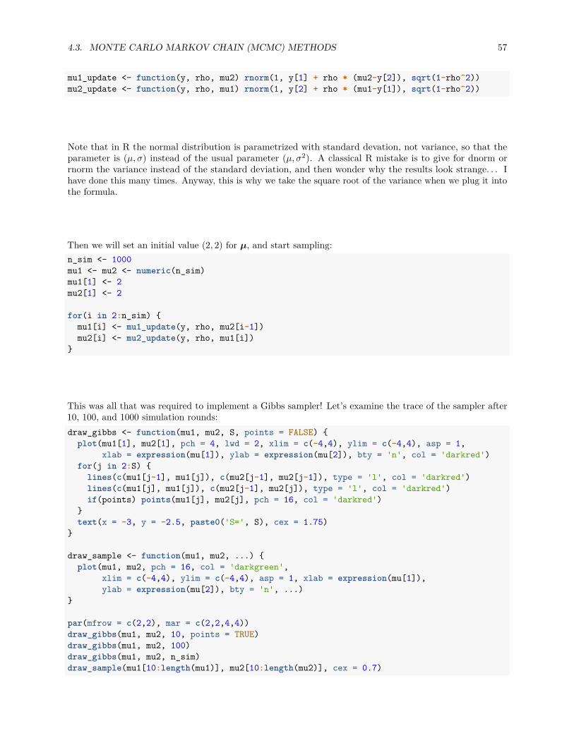
4.3. MONTE CARLO MARKOV CHAIN (MCMC) METHODS 57
mu1_update <- function(y, rho, mu2) rnorm(1, y[1] + rho * (mu2-y[2]), sqrt(1-rho^2))mu2_update <- function(y, rho, mu1) rnorm(1, y[2] + rho * (mu1-y[1]), sqrt(1-rho^2))
Note that in R the normal distribution is parametrized with standard devation, not variance, so that theparameter is (µ, σ) instead of the usual parameter (µ, σ2). A classical R mistake is to give for dnorm orrnorm the variance instead of the standard deviation, and then wonder why the results look strange. . . Ihave done this many times. Anyway, this is why we take the square root of the variance when we plug it intothe formula.
Then we will set an initial value (2, 2) for µ, and start sampling:n_sim <- 1000mu1 <- mu2 <- numeric(n_sim)mu1[1] <- 2mu2[1] <- 2
for(i in 2:n_sim) mu1[i] <- mu1_update(y, rho, mu2[i-1])mu2[i] <- mu2_update(y, rho, mu1[i])
This was all that was required to implement a Gibbs sampler! Let’s examine the trace of the sampler after10, 100, and 1000 simulation rounds:draw_gibbs <- function(mu1, mu2, S, points = FALSE)
plot(mu1[1], mu2[1], pch = 4, lwd = 2, xlim = c(-4,4), ylim = c(-4,4), asp = 1,xlab = expression(mu[1]), ylab = expression(mu[2]), bty = 'n', col = 'darkred')
for(j in 2:S) lines(c(mu1[j-1], mu1[j]), c(mu2[j-1], mu2[j-1]), type = 'l', col = 'darkred')lines(c(mu1[j], mu1[j]), c(mu2[j-1], mu2[j]), type = 'l', col = 'darkred')if(points) points(mu1[j], mu2[j], pch = 16, col = 'darkred')
text(x = -3, y = -2.5, paste0('S=', S), cex = 1.75)
draw_sample <- function(mu1, mu2, ...) plot(mu1, mu2, pch = 16, col = 'darkgreen',
xlim = c(-4,4), ylim = c(-4,4), asp = 1, xlab = expression(mu[1]),ylab = expression(mu[2]), bty = 'n', ...)
par(mfrow = c(2,2), mar = c(2,2,4,4))draw_gibbs(mu1, mu2, 10, points = TRUE)draw_gibbs(mu1, mu2, 100)draw_gibbs(mu1, mu2, n_sim)draw_sample(mu1[10:length(mu1)], mu2[10:length(mu2)], cex = 0.7)
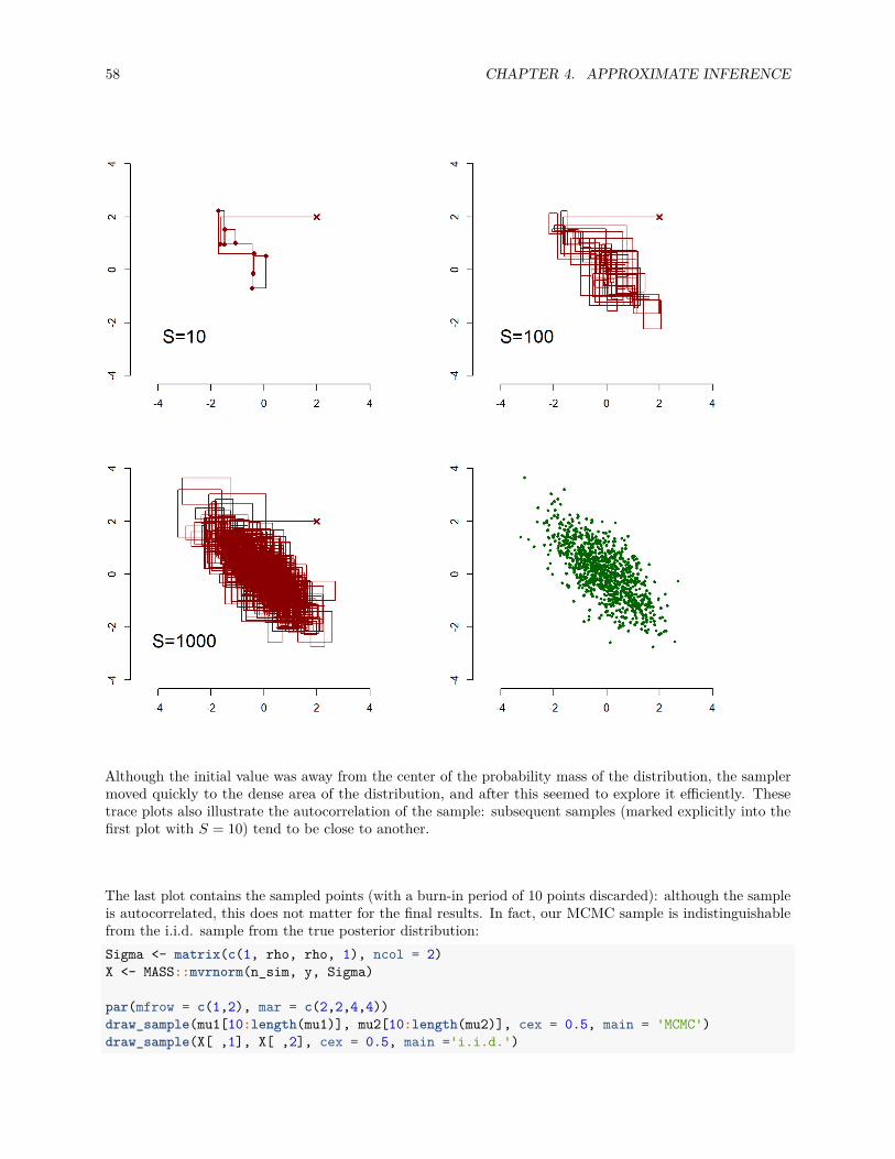
58 CHAPTER 4. APPROXIMATE INFERENCE
Although the initial value was away from the center of the probability mass of the distribution, the samplermoved quickly to the dense area of the distribution, and after this seemed to explore it efficiently. Thesetrace plots also illustrate the autocorrelation of the sample: subsequent samples (marked explicitly into thefirst plot with S = 10) tend to be close to another.
The last plot contains the sampled points (with a burn-in period of 10 points discarded): although the sampleis autocorrelated, this does not matter for the final results. In fact, our MCMC sample is indistinguishablefrom the i.i.d. sample from the true posterior distribution:Sigma <- matrix(c(1, rho, rho, 1), ncol = 2)X <- MASS::mvrnorm(n_sim, y, Sigma)
par(mfrow = c(1,2), mar = c(2,2,4,4))draw_sample(mu1[10:length(mu1)], mu2[10:length(mu2)], cex = 0.5, main = 'MCMC')draw_sample(X[ ,1], X[ ,2], cex = 0.5, main ='i.i.d.')
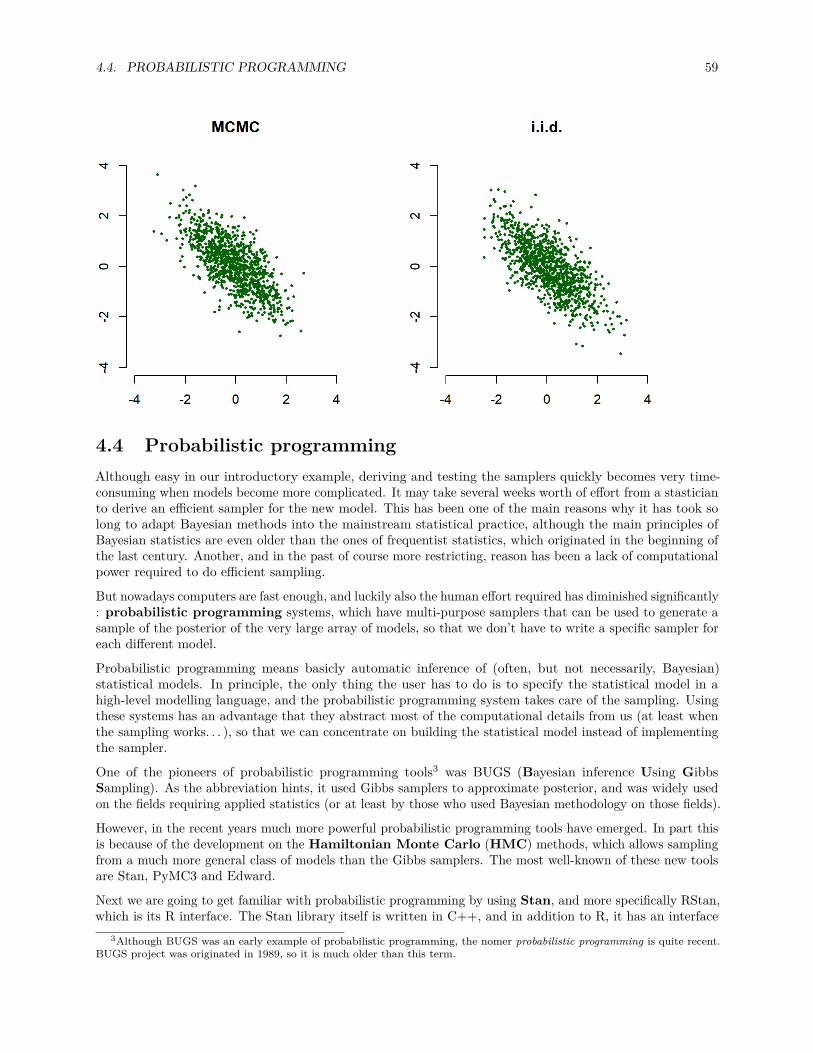
4.4. PROBABILISTIC PROGRAMMING 59
4.4 Probabilistic programmingAlthough easy in our introductory example, deriving and testing the samplers quickly becomes very time-consuming when models become more complicated. It may take several weeks worth of effort from a stasticianto derive an efficient sampler for the new model. This has been one of the main reasons why it has took solong to adapt Bayesian methods into the mainstream statistical practice, although the main principles ofBayesian statistics are even older than the ones of frequentist statistics, which originated in the beginning ofthe last century. Another, and in the past of course more restricting, reason has been a lack of computationalpower required to do efficient sampling.
But nowadays computers are fast enough, and luckily also the human effort required has diminished significantly: probabilistic programming systems, which have multi-purpose samplers that can be used to generate asample of the posterior of the very large array of models, so that we don’t have to write a specific sampler foreach different model.
Probabilistic programming means basicly automatic inference of (often, but not necessarily, Bayesian)statistical models. In principle, the only thing the user has to do is to specify the statistical model in ahigh-level modelling language, and the probabilistic programming system takes care of the sampling. Usingthese systems has an advantage that they abstract most of the computational details from us (at least whenthe sampling works. . . ), so that we can concentrate on building the statistical model instead of implementingthe sampler.
One of the pioneers of probabilistic programming tools3 was BUGS (Bayesian inference Using GibbsSampling). As the abbreviation hints, it used Gibbs samplers to approximate posterior, and was widely usedon the fields requiring applied statistics (or at least by those who used Bayesian methodology on those fields).
However, in the recent years much more powerful probabilistic programming tools have emerged. In part thisis because of the development on the Hamiltonian Monte Carlo (HMC) methods, which allows samplingfrom a much more general class of models than the Gibbs samplers. The most well-known of these new toolsare Stan, PyMC3 and Edward.
Next we are going to get familiar with probabilistic programming by using Stan, and more specifically RStan,which is its R interface. The Stan library itself is written in C++, and in addition to R, it has an interface
3Although BUGS was an early example of probabilistic programming, the nomer probabilistic programming is quite recent.BUGS project was originated in 1989, so it is much older than this term.
60 CHAPTER 4. APPROXIMATE INFERENCE
also for Python (PyStan) and some other high-level languages.
Installing RStan requires little more tuning than installing a normal R package. Detailed instructions forinstalling RStan for your operating systems can be found from: RStan-Getting-Started. That being said,installing RStan for Linux or MacOS may also work by just running the following line in R:install.packages("rstan", repos = "https://cloud.r-project.org/", dependencies=TRUE)
However, your mileage may vary; and following the official instructions is anyway recommended to optimizethe compiling and running speed of Stan models.
4.4.1 Minimal Stan-example : model declarationNow that you have installed Stan, all the hard work is done: fortunately using it fun and easy! When tryingnew software, I like to run a minimal “Hello World!”-example just to check that everything is set up andworking correctly. So as a “Stan - Hello world!” - example, let’s revisit Example 2.1.1 (Poisson samplingdistribution with gamma prior) again, and this time use Stan to simulate from the posterior.
Stan models are specified using a high-level modeling language whose syntax resembles R syntax. Models arewritten into their own .stan-files, which Stan first translates into C++ code and then compiles. Let’s startwriting our model into a new file, which we can name for example as poisson.stan.
A stan model consists of named blocks which are written inside the curly brackets. In principle all the blocksare optional, but three necessary blocks to specify a non-trivial probability model are data, parameters, andmodel.
First we need to declare the variables for the input data of our model into the data-block:
data int<lower=0> n;int<lower=0> y[n];
We declared a sample size n as a non-negative integer, and y as a vector of non-negative integers having ncomponents. Note that unlike in R syntax, we had to specify data types of the variables we are declaring;and in addition to specifying our variables as integers, we also constrained them to be non-negative integerswith the speficier lower=0. We could have also constrained our variable into a certain interval: for examplewe could declare the observation y from the binomial distribution Bin(n, θ), which is constrained into theinterval (0, n), as follows:
int<lower=0,upper=n> y;
Constraining the variables correctly (so that they are constrained to the support of their distribution4) isespecially important when declaring the parameters, because Stan uses these constraints when sampling.
Notice also that unlike in R or Python, but like in C++ or Java, each line ends with a semicolon. Omittingit is a syntax error.
Next we declare the parameters of the model in the parameters-block:
parameters real<lower=0> lambda;
Parameter of the Poisson(λ) distribution is a real number, so we declare its type as real. Note that we donot declare the hyperparameters of the prior Gamma(α, β)-distribution in the parameters-block, because weconsider them as fixed constants (here α = 1, β = 1), not as random variables like λ.
Finally, we specify our probability model in the model-block:4Support of the continuous probability distribution is a set where its density is positive.
4.4. PROBABILISTIC PROGRAMMING 61
model lambda ~ gamma(1,1);y ~ poisson(lambda);
Compare this to our usual model declaration:
Yi ∼ Poisson(λ) for all i = 1, . . . , nλ ∼ Gamma(1, 1)
Look pretty similar, right? Stan declaration is even a bit simpler, because Stan supports vectorization: astatement
y ~ poisson(lambda);
for the vector y means that each component of this vector follows Poisson(λ)-distribution. We could havealso used a more explicit and verbose form:
for(i in 1:n)y[i] ~ poisson(lambda);
A syntax of the for loop is similar to R. The body of the loop is enclosed in the curly brackets; if it consistsonly of one line, as above, these curly brackets can be omitted.
Our first two blocks consist of only variable declarations. The model-block is different: it containsstatements. The statements of the form
y ~ poisson(lambda);
are called sampling statements. They simply tell Stan which probability distribution our variables follow;these sampling statements are used to implement the sampler for the model.
Stan supports most of the well-known distributions, and it is also possible to define own probabilitydistributions by supplying its log-density function. A full list of the available distributions (and tons of otherinformation) can be found from Stan reference manual.
So our full stan model, which we save into the file poisson.stan, is:
data int<lower=0> n;int<lower=0> y[n];
parameters real<lower=0> lambda;
model lambda ~ gamma(1,1);y ~ poisson(lambda);
4.4.2 Minimal Stan-example : samplingWe have now specified our model and are ready to generate a sample from the posterior. But let’s firstgenerate our old data set y:lambda_true <- 3n_sample <- 5set.seed(111111)(y <- rpois(n, lambda_true))
62 CHAPTER 4. APPROXIMATE INFERENCE
## [1] 4 3 11 3 6
Then we wrap our observations and sample size into a list, which has components with the names correspondingto the variables declared in data-block of the Stan model:poisson_dat <- list(y = y, n = n_sample)
We have not yet loaded a package RStan, so let’s do it now:library(rstan)
Hmm, it recommends to run some code, so let’s do it:rstan_options(auto_write = TRUE)options(mc.cores = parallel::detectCores())
The first line allows saving the compiled model to the hard disk, so it saves time because the model doesnot has to be recompiled every time it is used. The second line allows Stan to run several Markov chains inparallel, which also saves time.
Now we are finally ready for the actual sampling. The sampling is done via stan-function. The followingcode works if the poisson.stan-file that contains the model is in your working directory:fit <- stan(file = 'poisson.stan', data = poisson_dat)# I cut the compiler and sampler messages from here to make this look more clean
Function stan first compiles the model, then draws a sample from the posterior, and finally returns thesampled values as stanfit object. Let’s print the summary of the returned stanfit-object:fit
## Inference for Stan model: poisson.## 4 chains, each with iter=2000; warmup=1000; thin=1;## post-warmup draws per chain=1000, total post-warmup draws=4000.#### mean se_mean sd 2.5% 25% 50% 75% 97.5% n_eff Rhat## lambda 4.67 0.02 0.87 3.10 4.06 4.64 5.21 6.52 1447 1## lp__ 14.64 0.02 0.69 12.72 14.49 14.91 15.08 15.13 2064 1#### Samples were drawn using NUTS(diag_e) at Mon Dec 18 09:35:51 2017.## For each parameter, n_eff is a crude measure of effective sample size,## and Rhat is the potential scale reduction factor on split chains (at## convergence, Rhat=1).
Stan runs as default 4 chains for 2000 iterations each, and it discards first half of the iterations as the warm-upperiod. So the default sample size is 4000, as shown above. Stan reports mean, median and 50% and 95%equal-tailed credible interval for our parameters of interest, in this case λ.
You can also run function stan without specifying the argument data. In case you omit this argument, Stantries to find the input data (variables y and n) from the global R enviroment. With our model this wouldprobably fail, because we have defined a sample size using the variable n_sample, not the variable n. Or thenit would be pick some n we have defined earlier in our code, which may or may not be correct. So it is muchmore clear and less error-prone to specify the input data explicitly as a list.
4.4.3 Minimal Stan example : illustrating the resultsWe can draw a boxplot of the simulated posterior distribution of the parameter λ simply as:plot(fit)
## ci_level: 0.8 (80% intervals)
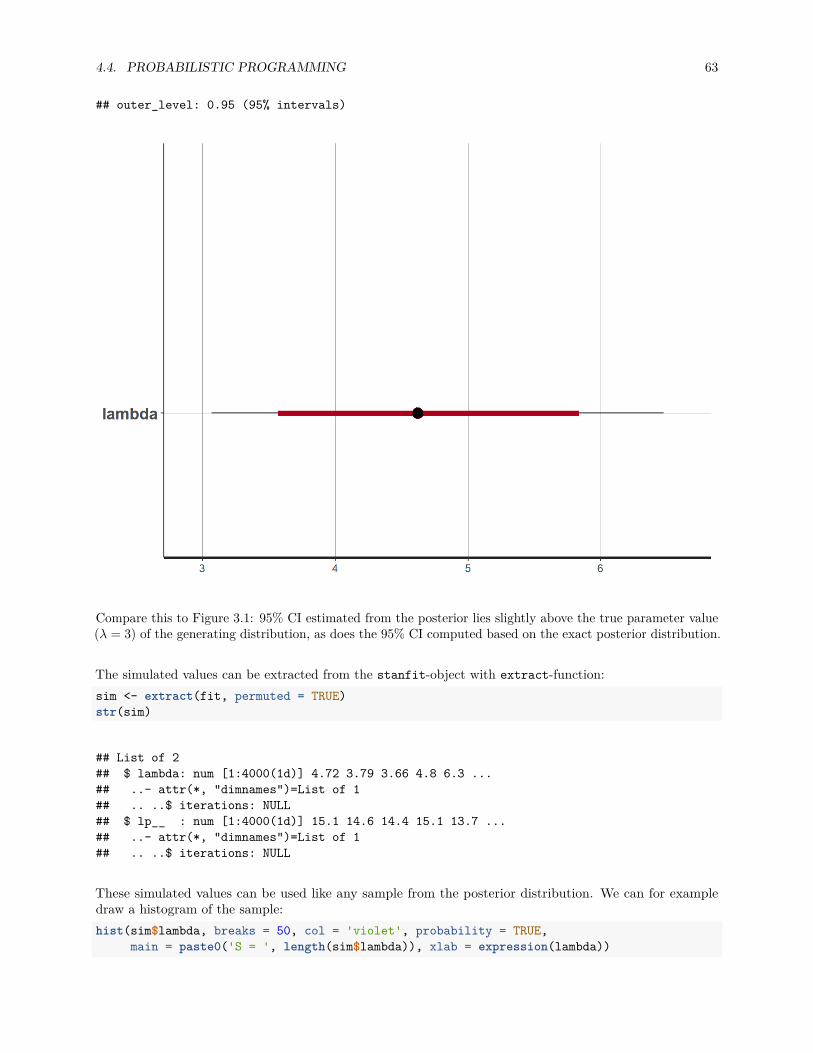
4.4. PROBABILISTIC PROGRAMMING 63
## outer_level: 0.95 (95% intervals)
Compare this to Figure 3.1: 95% CI estimated from the posterior lies slightly above the true parameter value(λ = 3) of the generating distribution, as does the 95% CI computed based on the exact posterior distribution.
The simulated values can be extracted from the stanfit-object with extract-function:sim <- extract(fit, permuted = TRUE)str(sim)
## List of 2## $ lambda: num [1:4000(1d)] 4.72 3.79 3.66 4.8 6.3 ...## ..- attr(*, "dimnames")=List of 1## .. ..$ iterations: NULL## $ lp__ : num [1:4000(1d)] 15.1 14.6 14.4 15.1 13.7 ...## ..- attr(*, "dimnames")=List of 1## .. ..$ iterations: NULL
These simulated values can be used like any sample from the posterior distribution. We can for exampledraw a histogram of the sample:hist(sim$lambda, breaks = 50, col = 'violet', probability = TRUE,
main = paste0('S = ', length(sim$lambda)), xlab = expression(lambda))
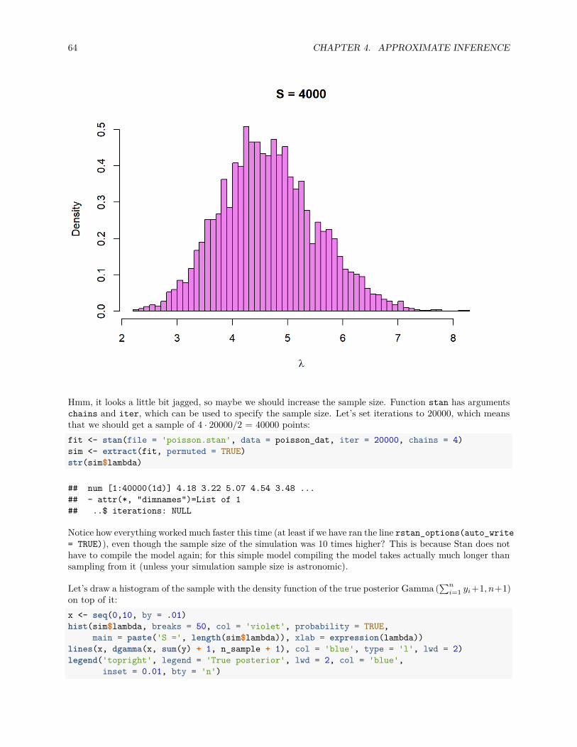
64 CHAPTER 4. APPROXIMATE INFERENCE
Hmm, it looks a little bit jagged, so maybe we should increase the sample size. Function stan has argumentschains and iter, which can be used to specify the sample size. Let’s set iterations to 20000, which meansthat we should get a sample of 4 · 20000/2 = 40000 points:fit <- stan(file = 'poisson.stan', data = poisson_dat, iter = 20000, chains = 4)sim <- extract(fit, permuted = TRUE)str(sim$lambda)
## num [1:40000(1d)] 4.18 3.22 5.07 4.54 3.48 ...## - attr(*, "dimnames")=List of 1## ..$ iterations: NULL
Notice how everything worked much faster this time (at least if we have ran the line rstan_options(auto_write= TRUE)), even though the sample size of the simulation was 10 times higher? This is because Stan does nothave to compile the model again; for this simple model compiling the model takes actually much longer thansampling from it (unless your simulation sample size is astronomic).
Let’s draw a histogram of the sample with the density function of the true posterior Gamma (∑ni=1 yi+1, n+1)
on top of it:x <- seq(0,10, by = .01)hist(sim$lambda, breaks = 50, col = 'violet', probability = TRUE,
main = paste('S =', length(sim$lambda)), xlab = expression(lambda))lines(x, dgamma(x, sum(y) + 1, n_sample + 1), col = 'blue', type = 'l', lwd = 2)legend('topright', legend = 'True posterior', lwd = 2, col = 'blue',
inset = 0.01, bty = 'n')
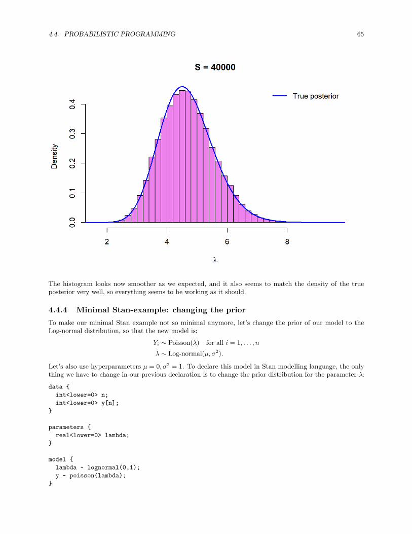
4.4. PROBABILISTIC PROGRAMMING 65
The histogram looks now smoother as we expected, and it also seems to match the density of the trueposterior very well, so everything seems to be working as it should.
4.4.4 Minimal Stan-example: changing the priorTo make our minimal Stan example not so minimal anymore, let’s change the prior of our model to theLog-normal distribution, so that the new model is:
Yi ∼ Poisson(λ) for all i = 1, . . . , nλ ∼ Log-normal(µ, σ2).
Let’s also use hyperparameters µ = 0, σ2 = 1. To declare this model in Stan modelling language, the onlything we have to change in our previous declaration is to change the prior distribution for the parameter λ:
data int<lower=0> n;int<lower=0> y[n];
parameters real<lower=0> lambda;
model lambda ~ lognormal(0,1);y ~ poisson(lambda);
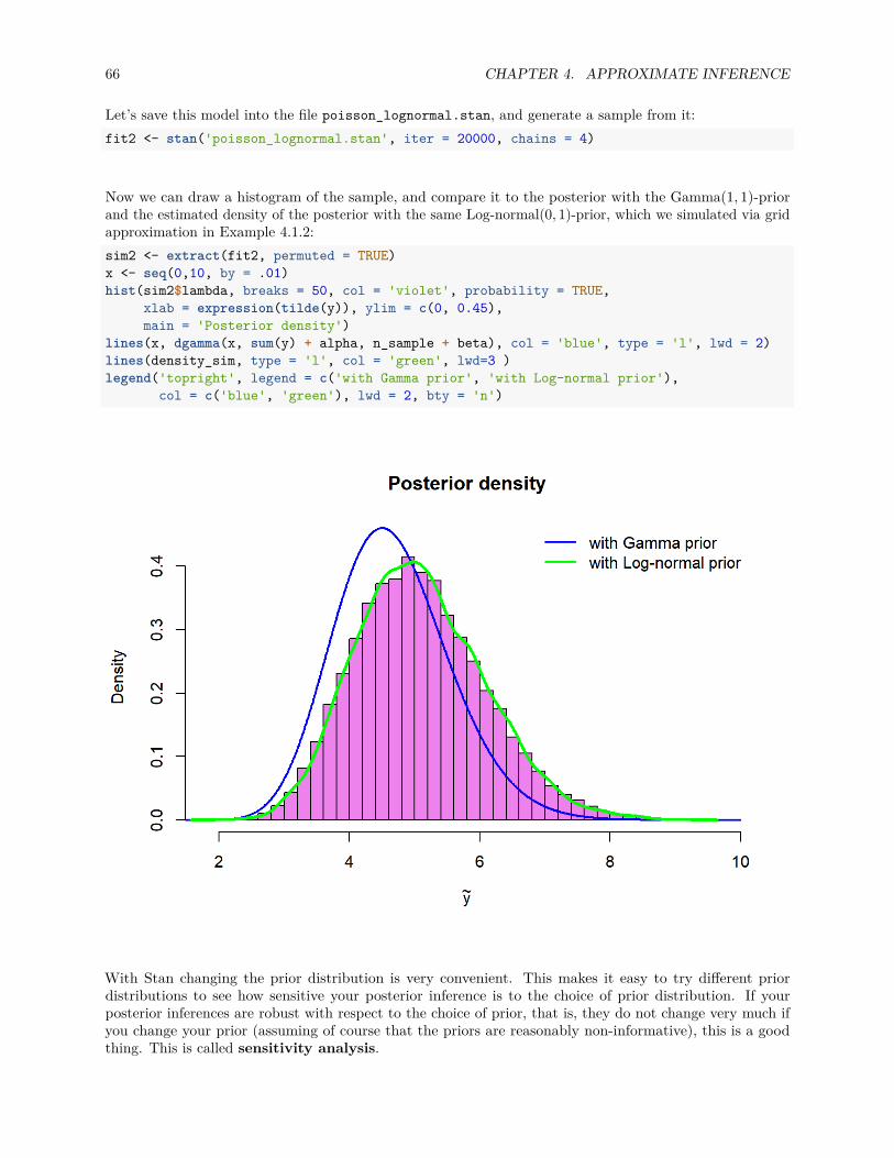
66 CHAPTER 4. APPROXIMATE INFERENCE
Let’s save this model into the file poisson_lognormal.stan, and generate a sample from it:fit2 <- stan('poisson_lognormal.stan', iter = 20000, chains = 4)
Now we can draw a histogram of the sample, and compare it to the posterior with the Gamma(1, 1)-priorand the estimated density of the posterior with the same Log-normal(0, 1)-prior, which we simulated via gridapproximation in Example 4.1.2:sim2 <- extract(fit2, permuted = TRUE)x <- seq(0,10, by = .01)hist(sim2$lambda, breaks = 50, col = 'violet', probability = TRUE,
xlab = expression(tilde(y)), ylim = c(0, 0.45),main = 'Posterior density')
lines(x, dgamma(x, sum(y) + alpha, n_sample + beta), col = 'blue', type = 'l', lwd = 2)lines(density_sim, type = 'l', col = 'green', lwd=3 )legend('topright', legend = c('with Gamma prior', 'with Log-normal prior'),
col = c('blue', 'green'), lwd = 2, bty = 'n')
With Stan changing the prior distribution is very convenient. This makes it easy to try different priordistributions to see how sensitive your posterior inference is to the choice of prior distribution. If yourposterior inferences are robust with respect to the choice of prior, that is, they do not change very much ifyou change your prior (assuming of course that the priors are reasonably non-informative), this is a goodthing. This is called sensitivity analysis.
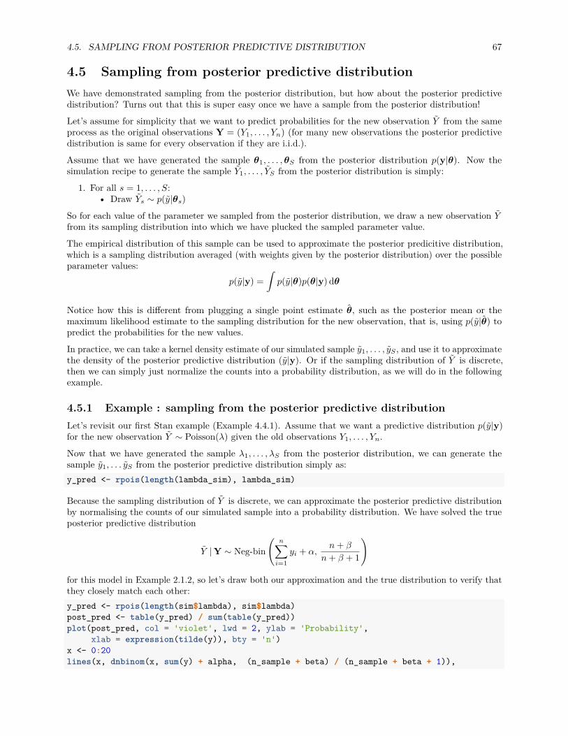
4.5. SAMPLING FROM POSTERIOR PREDICTIVE DISTRIBUTION 67
4.5 Sampling from posterior predictive distributionWe have demonstrated sampling from the posterior distribution, but how about the posterior predictivedistribution? Turns out that this is super easy once we have a sample from the posterior distribution!
Let’s assume for simplicity that we want to predict probabilities for the new observation Y from the sameprocess as the original observations Y = (Y1, . . . , Yn) (for many new observations the posterior predictivedistribution is same for every observation if they are i.i.d.).
Assume that we have generated the sample θ1, . . . ,θS from the posterior distribution p(y|θ). Now thesimulation recipe to generate the sample Y1, . . . , YS from the posterior distribution is simply:
1. For all s = 1, . . . , S:• Draw Ys ∼ p(y|θs)
So for each value of the parameter we sampled from the posterior distribution, we draw a new observation Yfrom its sampling distribution into which we have plucked the sampled parameter value.
The empirical distribution of this sample can be used to approximate the posterior predicitive distribution,which is a sampling distribution averaged (with weights given by the posterior distribution) over the possibleparameter values:
p(y|y) =∫p(y|θ)p(θ|y)dθ
Notice how this is different from plugging a single point estimate θ, such as the posterior mean or themaximum likelihood estimate to the sampling distribution for the new observation, that is, using p(y|θ) topredict the probabilities for the new values.
In practice, we can take a kernel density estimate of our simulated sample y1, . . . , yS , and use it to approximatethe density of the posterior predictive distribution (y|y). Or if the sampling distribution of Y is discrete,then we can simply just normalize the counts into a probability distribution, as we will do in the followingexample.
4.5.1 Example : sampling from the posterior predictive distributionLet’s revisit our first Stan example (Example 4.4.1). Assume that we want a predictive distribution p(y|y)for the new observation Y ∼ Poisson(λ) given the old observations Y1, . . . , Yn.
Now that we have generated the sample λ1, . . . , λS from the posterior distribution, we can generate thesample y1, . . . yS from the posterior predictive distribution simply as:y_pred <- rpois(length(lambda_sim), lambda_sim)
Because the sampling distribution of Y is discrete, we can approximate the posterior predictive distributionby normalising the counts of our simulated sample into a probability distribution. We have solved the trueposterior predictive distribution
Y |Y ∼ Neg-bin(
n∑i=1
yi + α,n+ β
n+ β + 1
)
for this model in Example 2.1.2, so let’s draw both our approximation and the true distribution to verify thatthey closely match each other:y_pred <- rpois(length(sim$lambda), sim$lambda)post_pred <- table(y_pred) / sum(table(y_pred))plot(post_pred, col = 'violet', lwd = 2, ylab = 'Probability',
xlab = expression(tilde(y)), bty = 'n')x <- 0:20lines(x, dnbinom(x, sum(y) + alpha, (n_sample + beta) / (n_sample + beta + 1)),
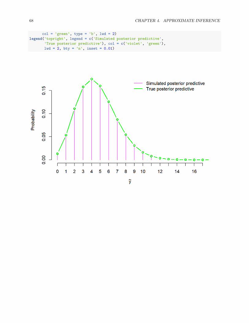
68 CHAPTER 4. APPROXIMATE INFERENCE
col = 'green', type = 'b', lwd = 2)legend('topright', legend = c('Simulated posterior predictive',
'True posterior predictive'), col = c('violet', 'green'),lwd = 2, bty = 'n', inset = 0.01)
Chapter 5
Multiparameter models
We have actually already examined computing the posterior distribution for the multiparameter modelbecause we have made an assumption that the parameter θ = (θ1, . . . , θd) is a d-component vector, andexamined one-dimensional parameter θ as a special case of this.
For instance, in the exercises we computed a posterior distribution for the parameter θ of the multinomialdistribution Multinom(n,θ). We were interested in the values of the whole parameter vector θ = (θ1, . . . , θd):this means that the full posterior distribution p(θ|y) was the desired result. This situation did not in principlediffer from the one-dimensional case.
However, often we are not interested in the full posterior p(θ|y), but only in the marginal posterior distributionsof some of the components of the parameter vector.
A classical example is a case in which we are interested in measuring some quantity, for example the speed oflight, and model our measurements Y1, . . . , Yn of the value of this quantity as an independent sample fromthe normal distribution:
Yi ∼ N(µ, σ2) for all i = 1, . . . , n.Now the parameter θ = (µ, σ2) of the model is two-dimensional, but sometimes we are only interested in thetrue value of the quantity µ, and not so much on our measurement error σ2. The parameter σ2 is called anuisance parameter here.
More generally, we will consider a situation in which the parameter vector θ = (θ1,θ2) is partitioned intotwo (possibly also vector-valued) components, θ1 being the parameter of interest, and θ2 being the nuisanceparameter.
5.1 Marginal posterior distributionAssume the partition of the parameter vector into two components: θ = (θ1,θ2). A distribution p(θ1|y)of the parameter of interest1 given the data is called a marginal posterior distribution, and it can becomputed by integrating the nuisance parameter out of the full posterior distribution:
p(θ1|y) =∫p(θ|y)dθ2
This integral can also be written as
p(θ1|y) =∫p(θ1,θ2|y)dθ2
=∫p(θ1|θ2,y)p(θ2|y)dθ2.
1Here we refer to θ1 as the parameter of interest and to θ2 as the nuisance parameter because of the clarity of presentation,but of course θ = (θ1, θ2) can be any partition of the parameter vector.
69
70 CHAPTER 5. MULTIPARAMETER MODELS
A distribution p(θ1|θ2,y) is called a conditional posterior distribution of the parameter θ1; the aboveintegral can be seen as an weighted average of the conditional posterior distribution, where the weights aregiven by the marginal posterior distribution of the nuisance parameter θ2.
5.2 Inference for the normal distribution with known varianceThe normal distribution is ubiquitous in the statistics and machine learning models, and it is also a niceexample of the multiparameter inference, because its parameter is two-dimensional θ = (θ, σ2), where often(but not always) an expected value θ is considered a parameter of interest, and a variance σ2 is considered anuisance parameter. Thus, we will go through the posterior inference for the normal model distribution hereas an example of the multiparameter inference.
However, before going to the actual multiparameter inference, we will consider a simpler example where weassume the variance σ2
0 of the normal distribution fixed. This is actually an example of the one-parameterconjugate model, because the only unknown parameter is the expected value θ of the distribution.
The posterior distribution for the inverse case in which the expected value is assumed to be known, but thevariance is unknown, was derived in the exercises. These simple models in which one of the parameters isfixed are useful for deriving the conditional posterior distributions in the case where both the mean andvariance are unknown.
5.2.1 One observationAssume first that we have one observation Y from the normal distribution with an unknown mean θ and afixed variance σ2
0 > 0. A conjugate distribution for this model is a normal distribution, so that the full modelis:
Y ∼ N(θ, σ20)
θ ∼ N(µ0, τ0).
The likelihood of this model can be written as
p(y|θ) = 1√2πσ2
0exp
(− (y − θ)2
2σ20
)∝ exp
(−θ
2 − 2yθ2σ2
0
),
and the prior distribution as
p(θ) = 1√2πτ2
0exp
(− (θ − µ0)2
2τ20
)∝ exp
(−θ
2 − 2µ0θ
2τ20
).
In both the likelihood and the prior the term in the exponent is a quadratic function of the parameter θ, sothis looks promising: we only have to recognize the same quadratic form of θ from the posterior to see thatit is a normal distribution. Let’s write the unnormalized posterior using the Bayes formula to find out theparameters of the posterior distribution:
p(θ|y) ∝ p(y|θ)p(θ)
∝ exp(−θ
2 − 2µ0θ
2τ20
− θ2 − 2yθ2σ2
0
)= exp
(−σ
20(θ2 − 2µ0θ) + τ2
0 (θ2 − 2yθ)2τ2
0σ20
)∝ exp
(− (σ2
0 + τ20 )θ2 − 2(σ2
0µ0 + τ20 y)θ
2τ20σ
20
)∝ exp
(−θ
2 − 2µ1θ
2τ21
),
5.2. INFERENCE FOR THE NORMAL DISTRIBUTION WITH KNOWN VARIANCE 71
where
µ1 = σ20µ0 + τ2
0 y
σ20 + τ2
0,
and
τ21 = τ2
0σ20
σ20 + τ2
0.
This means that the posterior distribution of the parameter θ is the normal distribution
θ |Y = y ∼ N(µ1, τ21 ).
We can also write the parameters of the posterior distribution by using the precision, which is an inverse ofthe variance 1/τ2. The posterior precision can be written as a sum of the prior precision and the samplingprecision (which was assumed to be a known constant):
1τ21
= 1τ20
+ 1σ2
0,
and the posterior mean can be written as a convex combination of the prior mean and the value of the onlyobservation:
µ1 =1τ2
0µ0 + 1
σ20y
1τ2
0+ 1
σ20
,
where the weights are the prior and the sampling precision.
5.2.2 Many observationsIn the previous example we derived the posterior distribution for the normal model with only one observation.But of course usually we have several observations, in which case the full model is:
Yi ∼ N(θ, σ2) for all i = 1, . . . , n,θ ∼ N(µ0, τ
2).
By repeating the above derivation, this time using the joint likelihood p(y|θ) =∏ni=1 p(yi|θ) instead of the
likelihood of the single observation, or by using the previous result and the fact that the mean of the normallydistributed random variables has a normal distribution
Y ∼ N(θ, σ2/n),
(and that the sample mean y is a so called sufficient statistic for this model) we can see that the posterior isthe normal distribution
θ |Y = y ∼ N(µn, τ2n),
where the expected value is
µn =1τ2
0µ0 + n
σ20y
1τ2
0+ n
σ20
,
and the precision is1τ2n
= 1τ20
+ n
σ20.
We can again see that the posterior mean is the convex combination of the prior mean and the mean of theobservations, and that the weight of the data mean is proportional to the number of observations: the higherthe sample size, the stonger the influence of the data on the posterior mean.
72 CHAPTER 5. MULTIPARAMETER MODELS
5.3 Inference for the normal distribution with noninformativeprior
Next we will consider the general case in which have again n observations from the normal distribution, butthis time both the mean µ and variance of the distribution are assumed unknown. Using a noninformativeimproper prior 1/σ2 for the parameter (µ, σ2) our full model is:
Yi ∼ N(µ, σ2) for all i = 1, . . . , n,
p(µ, σ2) ∝ 1σ2 .
First we will derive the full posterior distribution of this model, and using this full posterior derive themarginal posteriors for both the expected value µ and the variance σ2.
The general conjugate prior for this model is set hierarchically as:
µ |σ2 ∼ N(µ0, σ2/κ0),
σ2 ∼ Inv-χ2(ν0, σ20),
so that the joint prior for the parameters is
p(µ, σ2) ∝ (σ2)−(ν0+3)/2 exp−ν0σ
20 + κ0(µ0 − µ)2
2σ2
.
This distribution is called the normal inverse chi-squared distribution (NIX) and denoted as
(µ, σ2) ∼ N -Inv-χ2(µ0, σ20/κ0, ν0, σ
20).
We will show in the exercises that the full posterior distribution for the parameter (µ, σ2) is also of this form,but let’s first solve the joint posterior and the marginal posteriors in the special case of noninformative prior.
5.3.1 Full posteriorBy using the following factorization (this can be easily proven by writing the left hand side out and rearrangingterms):
n∑i=1
(yi − µ)2 =n∑i=1
(yi − y)2 + n(y − µ)2,
and the likelihood for n independent observations from the same normal distribution:
p(y|µ, σ2) =j∏i=1
p(yi|µ, σ2) ∝ σ−n exp−∑ni=1(yi − µ)2
2σ2
we can write the unnormalized join posterior distribution of both µ and σ2 as:
p(µ, σ2|y) ∝ p(µ, σ2)p(y|µ, σ2)
∝ σ−2 · σ−n exp−∑ni=1(yi − µ)2
2σ2
∝ σ−n−2 exp
−∑ni=1(yi − y)2 + n(y − µ)2
2σ2
∝ σ−n−2 exp
− (n− 1)s2 + n(y − µ)2
2σ2
,
where the sample mean
y = 1n
n∑i=1
yi
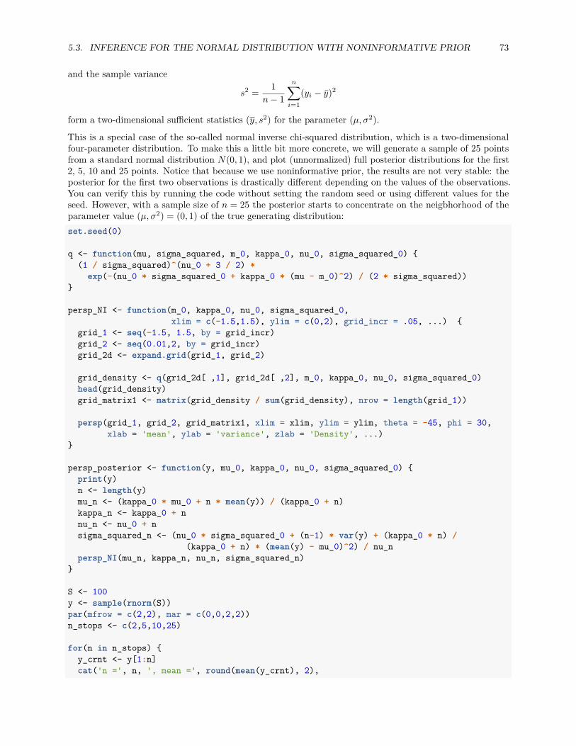
5.3. INFERENCE FOR THE NORMAL DISTRIBUTION WITH NONINFORMATIVE PRIOR 73
and the sample variance
s2 = 1n− 1
n∑i=1
(yi − y)2
form a two-dimensional sufficient statistics (y, s2) for the parameter (µ, σ2).
This is a special case of the so-called normal inverse chi-squared distribution, which is a two-dimensionalfour-parameter distribution. To make this a little bit more concrete, we will generate a sample of 25 pointsfrom a standard normal distribution N(0, 1), and plot (unnormalized) full posterior distributions for the first2, 5, 10 and 25 points. Notice that because we use noninformative prior, the results are not very stable: theposterior for the first two observations is drastically different depending on the values of the observations.You can verify this by running the code without setting the random seed or using different values for theseed. However, with a sample size of n = 25 the posterior starts to concentrate on the neigbhorhood of theparameter value (µ, σ2) = (0, 1) of the true generating distribution:set.seed(0)
q <- function(mu, sigma_squared, m_0, kappa_0, nu_0, sigma_squared_0) (1 / sigma_squared)^(nu_0 + 3 / 2) *
exp(-(nu_0 * sigma_squared_0 + kappa_0 * (mu - m_0)^2) / (2 * sigma_squared))
persp_NI <- function(m_0, kappa_0, nu_0, sigma_squared_0,xlim = c(-1.5,1.5), ylim = c(0,2), grid_incr = .05, ...)
grid_1 <- seq(-1.5, 1.5, by = grid_incr)grid_2 <- seq(0.01,2, by = grid_incr)grid_2d <- expand.grid(grid_1, grid_2)
grid_density <- q(grid_2d[ ,1], grid_2d[ ,2], m_0, kappa_0, nu_0, sigma_squared_0)head(grid_density)grid_matrix1 <- matrix(grid_density / sum(grid_density), nrow = length(grid_1))
persp(grid_1, grid_2, grid_matrix1, xlim = xlim, ylim = ylim, theta = -45, phi = 30,xlab = 'mean', ylab = 'variance', zlab = 'Density', ...)
persp_posterior <- function(y, mu_0, kappa_0, nu_0, sigma_squared_0) print(y)n <- length(y)mu_n <- (kappa_0 * mu_0 + n * mean(y)) / (kappa_0 + n)kappa_n <- kappa_0 + nnu_n <- nu_0 + nsigma_squared_n <- (nu_0 * sigma_squared_0 + (n-1) * var(y) + (kappa_0 * n) /
(kappa_0 + n) * (mean(y) - mu_0)^2) / nu_npersp_NI(mu_n, kappa_n, nu_n, sigma_squared_n)
S <- 100y <- sample(rnorm(S))par(mfrow = c(2,2), mar = c(0,0,2,2))n_stops <- c(2,5,10,25)
for(n in n_stops) y_crnt <- y[1:n]cat('n =', n, ', mean =', round(mean(y_crnt), 2),
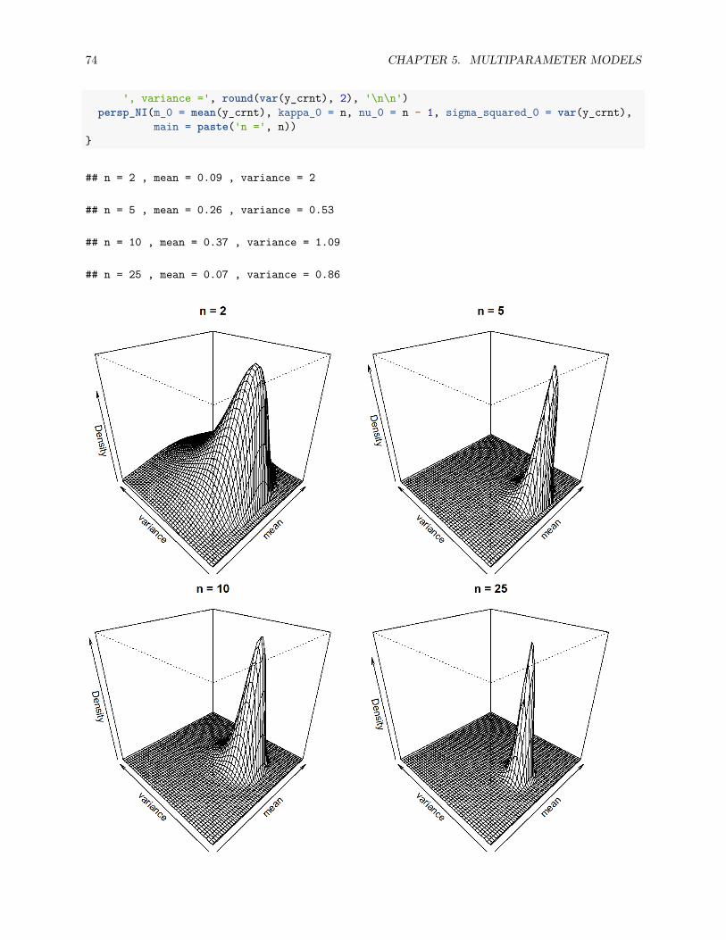
74 CHAPTER 5. MULTIPARAMETER MODELS
', variance =', round(var(y_crnt), 2), '\n\n')persp_NI(m_0 = mean(y_crnt), kappa_0 = n, nu_0 = n - 1, sigma_squared_0 = var(y_crnt),
main = paste('n =', n))
## n = 2 , mean = 0.09 , variance = 2
## n = 5 , mean = 0.26 , variance = 0.53
## n = 10 , mean = 0.37 , variance = 1.09
## n = 25 , mean = 0.07 , variance = 0.86
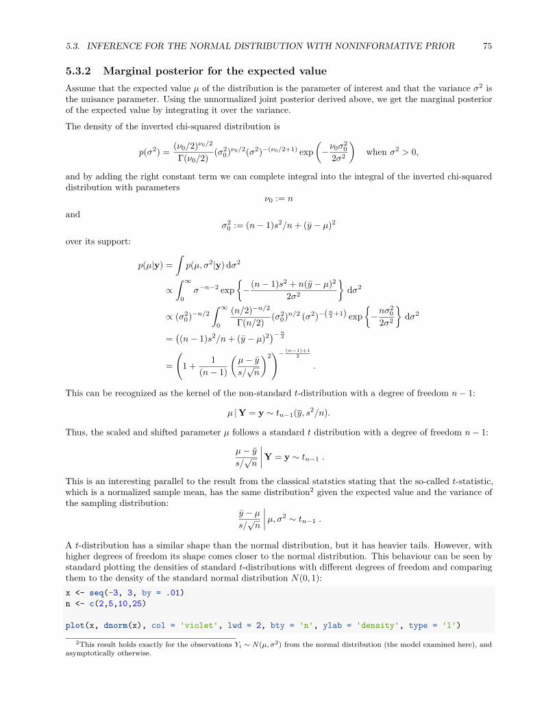
5.3. INFERENCE FOR THE NORMAL DISTRIBUTION WITH NONINFORMATIVE PRIOR 75
5.3.2 Marginal posterior for the expected valueAssume that the expected value µ of the distribution is the parameter of interest and that the variance σ2 isthe nuisance parameter. Using the unnormalized joint posterior derived above, we get the marginal posteriorof the expected value by integrating it over the variance.
The density of the inverted chi-squared distribution is
p(σ2) = (ν0/2)ν0/2
Γ(ν0/2) (σ20)ν0/2(σ2)−(ν0/2+1) exp
(−ν0σ
20
2σ2
)when σ2 > 0,
and by adding the right constant term we can complete integral into the integral of the inverted chi-squareddistribution with parameters
ν0 := n
andσ2
0 := (n− 1)s2/n+ (y − µ)2
over its support:
p(µ|y) =∫p(µ, σ2|y)dσ2
∝∫ ∞
0σ−n−2 exp
− (n− 1)s2 + n(y − µ)2
2σ2
dσ2
∝ (σ20)−n/2
∫ ∞0
(n/2)−n/2Γ(n/2) (σ2
0)n/2 (σ2)−(n2 +1) exp−nσ
20
2σ2
dσ2
=((n− 1)s2/n+ (y − µ)2)−n2
=(
1 + 1(n− 1)
(µ− ys/√n
)2)− (n−1)+1
2
.
This can be recognized as the kernel of the non-standard t-distribution with a degree of freedom n− 1:
µ |Y = y ∼ tn−1(y, s2/n).
Thus, the scaled and shifted parameter µ follows a standard t distribution with a degree of freedom n− 1:
µ− ys/√n
∣∣∣∣Y = y ∼ tn−1 .
This is an interesting parallel to the result from the classical statstics stating that the so-called t-statistic,which is a normalized sample mean, has the same distribution2 given the expected value and the variance ofthe sampling distribution:
y − µs/√n
∣∣∣∣µ, σ2 ∼ tn−1 .
A t-distribution has a similar shape than the normal distribution, but it has heavier tails. However, withhigher degrees of freedom its shape comes closer to the normal distribution. This behaviour can be seen bystandard plotting the densities of standard t-distributions with different degrees of freedom and comparingthem to the density of the standard normal distribution N(0, 1):x <- seq(-3, 3, by = .01)n <- c(2,5,10,25)
plot(x, dnorm(x), col = 'violet', lwd = 2, bty = 'n', ylab = 'density', type = 'l')
2This result holds exactly for the observations Yi ∼ N(µ, σ2) from the normal distribution (the model examined here), andasymptotically otherwise.
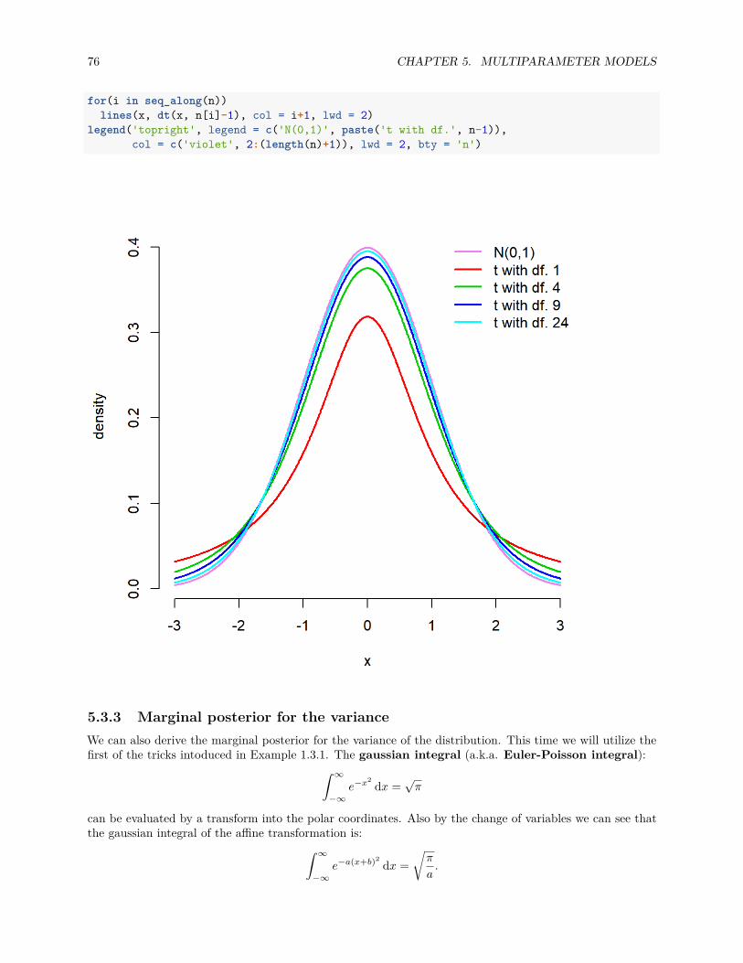
76 CHAPTER 5. MULTIPARAMETER MODELS
for(i in seq_along(n))lines(x, dt(x, n[i]-1), col = i+1, lwd = 2)
legend('topright', legend = c('N(0,1)', paste('t with df.', n-1)),col = c('violet', 2:(length(n)+1)), lwd = 2, bty = 'n')
5.3.3 Marginal posterior for the varianceWe can also derive the marginal posterior for the variance of the distribution. This time we will utilize thefirst of the tricks intoduced in Example 1.3.1. The gaussian integral (a.k.a. Euler-Poisson integral):∫ ∞
−∞e−x
2dx =
√π
can be evaluated by a transform into the polar coordinates. Also by the change of variables we can see thatthe gaussian integral of the affine transformation is:∫ ∞
−∞e−a(x+b)2
dx =√π
a.
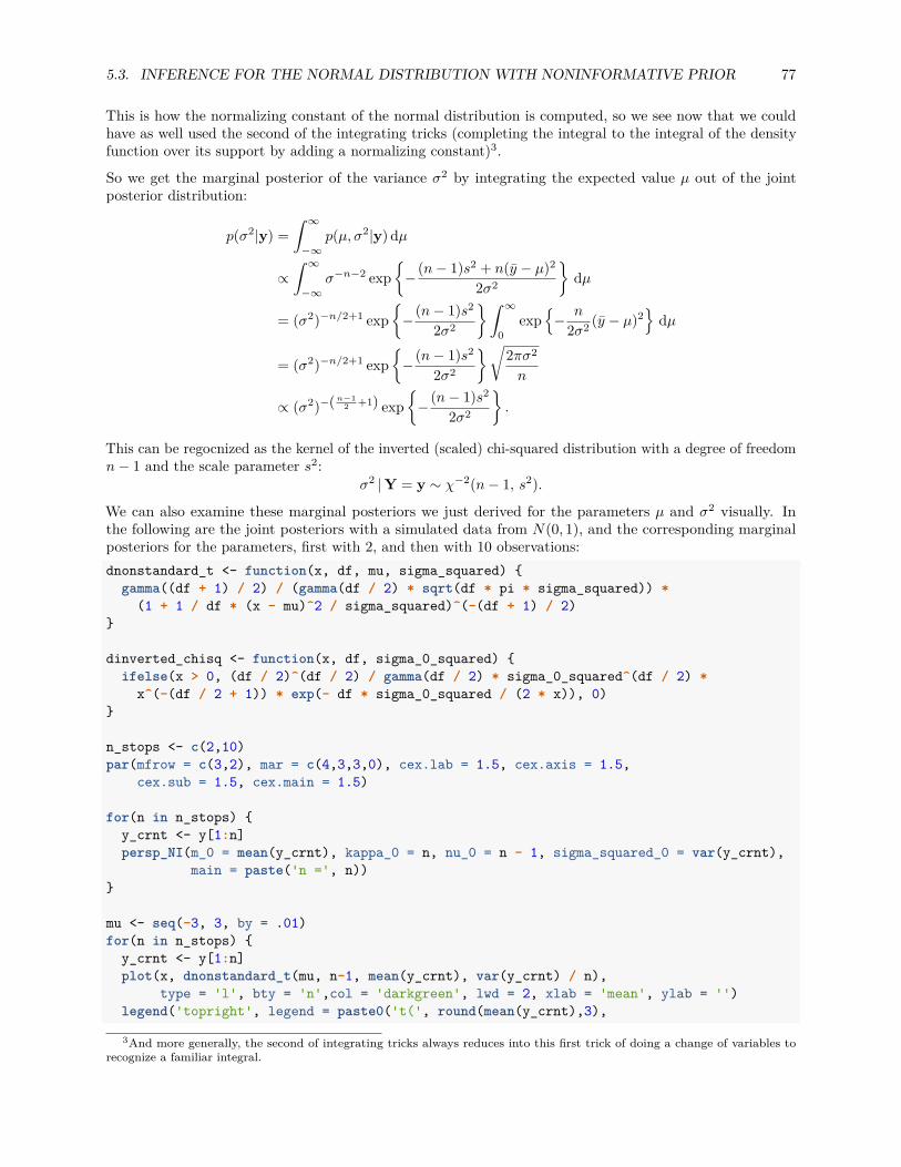
5.3. INFERENCE FOR THE NORMAL DISTRIBUTION WITH NONINFORMATIVE PRIOR 77
This is how the normalizing constant of the normal distribution is computed, so we see now that we couldhave as well used the second of the integrating tricks (completing the integral to the integral of the densityfunction over its support by adding a normalizing constant)3.
So we get the marginal posterior of the variance σ2 by integrating the expected value µ out of the jointposterior distribution:
p(σ2|y) =∫ ∞−∞
p(µ, σ2|y)dµ
∝∫ ∞−∞
σ−n−2 exp− (n− 1)s2 + n(y − µ)2
2σ2
dµ
= (σ2)−n/2+1 exp− (n− 1)s2
2σ2
∫ ∞0
exp− n
2σ2 (y − µ)2dµ
= (σ2)−n/2+1 exp− (n− 1)s2
2σ2
√2πσ2
n
∝ (σ2)−(n−12 +1) exp
− (n− 1)s2
2σ2
.
This can be regocnized as the kernel of the inverted (scaled) chi-squared distribution with a degree of freedomn− 1 and the scale parameter s2:
σ2 |Y = y ∼ χ−2(n− 1, s2).
We can also examine these marginal posteriors we just derived for the parameters µ and σ2 visually. Inthe following are the joint posteriors with a simulated data from N(0, 1), and the corresponding marginalposteriors for the parameters, first with 2, and then with 10 observations:dnonstandard_t <- function(x, df, mu, sigma_squared)
gamma((df + 1) / 2) / (gamma(df / 2) * sqrt(df * pi * sigma_squared)) *(1 + 1 / df * (x - mu)^2 / sigma_squared)^(-(df + 1) / 2)
dinverted_chisq <- function(x, df, sigma_0_squared) ifelse(x > 0, (df / 2)^(df / 2) / gamma(df / 2) * sigma_0_squared^(df / 2) *
x^(-(df / 2 + 1)) * exp(- df * sigma_0_squared / (2 * x)), 0)
n_stops <- c(2,10)par(mfrow = c(3,2), mar = c(4,3,3,0), cex.lab = 1.5, cex.axis = 1.5,
cex.sub = 1.5, cex.main = 1.5)
for(n in n_stops) y_crnt <- y[1:n]persp_NI(m_0 = mean(y_crnt), kappa_0 = n, nu_0 = n - 1, sigma_squared_0 = var(y_crnt),
main = paste('n =', n))
mu <- seq(-3, 3, by = .01)for(n in n_stops)
y_crnt <- y[1:n]plot(x, dnonstandard_t(mu, n-1, mean(y_crnt), var(y_crnt) / n),
type = 'l', bty = 'n',col = 'darkgreen', lwd = 2, xlab = 'mean', ylab = '')legend('topright', legend = paste0('t(', round(mean(y_crnt),3),
3And more generally, the second of integrating tricks always reduces into this first trick of doing a change of variables torecognize a familiar integral.
78 CHAPTER 5. MULTIPARAMETER MODELS
', ', round(var(y_crnt) / n, 3), ')\nwith df ', n-1),col = 'darkgreen', lwd = 2, bty = 'n', cex = 1.3)
sigma_grid <- seq(0,5, by = .01)for(n in n_stops)
y_crnt <- y[1:n]plot(sigma_grid, dinverted_chisq(sigma_grid, n-1, var(y_crnt)), ylab = '',
type = 'l', bty = 'n',col = 'darkred', lwd = 2, xlab = 'variance')legend('topright', legend = paste0('Inv-chisq(', n-1, ', ',
round(var(y_crnt), 3), ')'), col = 'darkred', lwd = 2, bty = 'n', cex = 1.3)
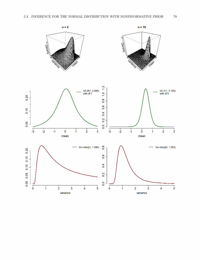
5.3. INFERENCE FOR THE NORMAL DISTRIBUTION WITH NONINFORMATIVE PRIOR 79

80 CHAPTER 5. MULTIPARAMETER MODELS
Chapter 6
Hierarchical models
Often observations have some kind of a natural hierarchy, so that the single observations can be modelledbelonging into different groups, which can also be modeled as being members of the common supergroup,and so on. For instance, the results of the survey may be grouped at the country, county, town or evenneighborhood level. This kind of the spatial hierarchy is the most concrete example of the hierarchy structure,but for example different clinical experiments on the effect of the same drug can be also modeled hierarchically:the results of each test subject belong to the one of the experiments (=groups), and these groups can bemodeled as a sample from the common population distribution. This kind of the combining of results of thedifferent studies on the same topic is called meta-analysis.
Often the observations inside one group can be modeled as independent: for instance, the results of thetest subjects of the randomized experiments, or responses of the survey participant chosen by the randomsampling can be reasonably thought to be independent. On the other hand, the parameters of the groups,for example mean response of the test subjects to the same drug in the different clinical experiments, canhardly be thought as independent. However, because the experimental conditions, for example the age orother attributes of the test subjects, length of the experiment and so on, are likely to affect the results, it alsodoes not feel right to assume the are no differences at all between the groups by pooling all the observationstogether.
The idea of the hierarchical modeling is to use the data to model the strength of the dependency betweenthe groups. The groups are assumed to be a sample from the underlying population distribution, andthe variance of this population distribution, which is estimated from the data, determines how much theparameters of the sampling distribution are shrunk towards the common mean.
First we will take a look at the general form of the two-level hierarchical model, and then make the discussionmore concrete by carefully examining a classical example of the hierarchical model.
6.1 Two-level hierarchical modelThe most basic two-level hierarchical model, where we have J groups, and n1, . . . nJ observations from eachof the groups, can be written as
Yij |θj ∼ p(yij |θj) for all i = 1, . . . , njθj |φ ∼ p(θj |φ) for all j = 1, . . . , J.
for each of the j = 1, . . . , J groups.
We assume that the observations Y1j , . . . , Ynjj within each group are i.i.d., so that the joint samplingdistribution can be written as a product of the sampling distributions of the single observations (which
81
82 CHAPTER 6. HIERARCHICAL MODELS
were assumed to be the same):
p(yj |θj) =nj∏i=1
p(yij |θj).
Group-level parameters (θ1, . . . ,θJ) are then modeled as an i.i.d. sample from the common populationdistribution p(θj |φ) so that their joint distribution can also be factorized as:
p(θ|φ) =J∏j=1
p(θj |φ).
The full model specification depends on how we handle the hyperparameters. We will introduce three options:
1. fix them to some constant values,2. use a point estimates estimated from the data or3. set a probability distribution over them.
When we speak about the Bayesian hierarchical models, we usually mean the third option, which meansspecifying the fully Bayesian model by setting the prior also for the hyperparameters.
6.1.1 No-pooling modelIf we just fix the hyperparameters to some fixed value φ = φ0, then the posterior distribution for theparameters θ simply factorizes to J components:
p(θ|y) ∝ p(θ|φ0)p(y|θ) =J∏j=1
p(θj |φ0)p(yj |θj),
because the prior distributions p(θj |φ0) were assumed as independent (we could also have removed theconditioning on the φ0 from the notation, because the hyperparameters are not assumed to be randomvariables in this model). Now all J components of the posterior distribution can be estimated separately; thismeans that we assume that the we do not model any dependency between the group-level parameters θj(expect for the common fixed prior distribution).
This option means specifying the non-hierarchical model by assuming the group-level parameters independent.It is prone to overfitting, especially if there is only little data on some of the groups, because it does not allowus to ‘’borrow statistical strength” for these groups with less data from the other more data-heavy groups.
6.1.2 Empirical BayesThe no-pooling model fixes the hyperparameters so that no information flows through them. However, wecan also avoid setting any distribution hyperparameters, while still letting the data dictate the strength ofthe dependency between the group-level parameters. This is done by approximating the hyperparameters bythe point estimates, more specifically fixing them to their maximum likelihood estimates, which are estimatedfrom the marginal likelihood of the data p(y|φ):
φMLE(y) = argmaxφ
p(y|φ) = argmaxφ
∫p(yj |θ)p(θ|φ)dθ.
This is why we computed the maximum likelihood estimate of the beta-binomial distribution in Problem 4 ofExercise set 3 (the problem of estimating the proportions of very liberals in each of the states): the marginallikelihood of the binomial distribution with beta prior is beta-binomial, and we wanted to find out maximumlikelihood estimates of the hyperparameters to apply the empirical Bayes procedure.
When the hyperparameters are fixed, we can factorize the posterior as in the no-pooling model:
p(θ|y) ∝ p(θ|φMLE)p(y|θ) =J∏j=1
p(θj |φMLE)p(yj |θj),
6.1. TWO-LEVEL HIERARCHICAL MODEL 83
and compute the posterior for each of the J components separately. This is why we could compute theposteriors for the proportions of very liberals separately for each of the states in the exercises.
Note that despite of the name, the empirical Bayes is not a Bayesian procedure, because the maximumlikelihood estimate is used. It is also a little bit of the ‘’double counting”, because the data is first used toestimate the parameters of the prior distribution, and then this prior and the data are used to computethe posterior for the group-level parameters. However, the empirical Bayes approach can be seen as acomputationally convenient approximation of the fully Bayesian model, because it avoids integrating over thehyperparameters. Also, often point estimates may be substituted for some of the parameters in the otherwiseBayesian model. We will actually do this for the within-group variances in our example of the hierarchicalmodel.
6.1.3 Fully Bayesian modelTo specify the fully Bayesian model, we set a prior distribution also for the hyperparameters, so that the fullmodel becomes:
Yij |θj ∼ p(yij |θj) for all i = 1, . . . , njθj |φ ∼ p(θj |φ) for all j = 1, . . . , J
φ ∼ p(φ).
We have already explicitly made the following conditional independence assumptions:
Y11, . . . , Yn11, . . . , Y1J , . . . , YnJJ ⊥⊥ |θθ1, . . . ,θJ ⊥⊥ |φ,
but the crucial implicit conditional independence assumption of the hierarchical model is that the datadepends on the hyperparameters only through the population level parameters:
Y ⊥⊥ φ |θ
This means that the sampling distribution of the observations given the populations parameters simplifies to
p(y|θ,φ) = p(y|θ),
and thus the full posterior over the parameters can be written using the Bayes formula:
p(θ,φ, |y) ∝ p(θ,φ)p(y|θ,φ)= p(φ)p(θ|φ)p(y|θ)
= p(φ)J∏j=1
p(θj |φ)p(yj |θj).
Because now the full posterior does not factorize anymore, we cannot solve the marginal posteriors of thegroup-level parameters p(θj |y) independently, and thus the whole model cannot be solved analytically.However, in the case of conditional conjugacy (which we will consider in the next section), we can mixsimulation and techniques for multi-parameter inference from Chapter 5 to derive the marginal posteriors.
Because the empirical Bayes approximates the marginal posterior of the group-level parameters by pluggingin the point estimates of the hyperparameters to the conditional posterior of the group-level parameters giventhe hyperparameters:
p(θ|y) ≈ p(θ|φMLE,y),
it underestimates the uncertainty coming from estimating the hyperparameters. In the fully Bayesianapproach the marginal posterior of the group-level parameters is obtained by integrating the conditionalposterior distribution of the group-level parameters over the whole marginal posterior distribution of the
84 CHAPTER 6. HIERARCHICAL MODELS
hyperparameters (i.e. by taking the expected value of the conditional posterior distribution of the group-levelparameters over the marginal posterior distribution of the hyperparameters):
p(θ|y) =∫p(θ,φ|y)dφ =
∫p(θ|φ,y)p(φ|y)dφ.
This means that the fully Bayesian model properly takes into account the uncertainty about the hyperparametervalues by averaging over their posterior.
In principle, this difference between the empirical Bayses and the full Bayes is the same as the differencebetween using the sampling distribution with a plug-in point estimate p(y|θMLE) and using the full properposterior predictive distribution p(y|y), which is derived by integrating the sampling distribution over theposterior distribution of the parameter, for predicting the new observations. In Murphy’s Murphy (2012)book there is a nice quote stating that ‘’the more we integrate, the more Bayesian we are. . . ”
6.2 Conditional conjugacyIf the population distribution p(θ|φ) is a conjugate distribution for the sampling distribution p(y|θ), thenwe talk about the conditional conjugacy, because the conditional posterior distribution of the populationparameters given the hyperparameters p(θ|y,φ) can be solved analytically1. Then simulating from themarginal posterior distribution of the hyperparameters p(φ|y) is usually a simple matter.
In the following example we could have utilized the conditional conjugacy, because the sampling distributionis a normal distribution with a fixed variance, and the population distribution is also a normal distribution.However, we take a fully simulational approach by directly generating a sample (φ(1),θ(1)), . . . , (φ(S),θ(S))from the full posterior p(θ,φ, |y). Then the components φ(1), . . . ,φ(S) can be used as a sample from themarginal posterior p(φ|y), and the components θ(1), . . . ,θ(S) can be used as a sample from the marginalposterior p(θ|y).
The downside of this approach is that the amount of time to compile the model and to sample from itusing Stan is orders of magnitudes greater than the time it would take to generate a sample from theposterior utilizing the conditional conjugacy. However, it takes only few minutes to write the model intoStan, whereas solving the part of the posterior analytically, and implementing a sampler for the rest wouldtake a considerably longer time for us to do. So it is a trade-off between the human and the computing effort,and this time we decide to delegate the job to the computer.
6.3 Hierarchical model exampleWe will consider a classical example of a Bayesian hierarchical model taken from the red book Gelman et al.(2013). The problem is to estimate the effectiviness of training programs different schools have for preparingtheir students for a SAT-V (scholastic aptitude test - verbal) test. SAT is designed to test the knowledgethat students have accumulated during their years at school, and the test scores should not be affected byshort term training programs. Nevertheless, each of the eight schools claim that their training programincreases the SAT scores of the students, and we want to find out what are the real effects of these trainingprograms. The data are not the raw scores of the students, but the training effects estimated on the basis ofthe preliminary SAT tests and SAT-M (scholastic aptitude test - mathematics) taken by the same students.You can read more about the experimental set-up from the section 5.5 of Gelman et al. (2013).
So there are in total J = 8 schools (=groups); in each of these schools we denote observed training effects ofthe students as Y1j , . . . , Ynjj . We will use the point estimates for the standard deviations σ2
j for each of theschools2.
1This is why we chose the beta prior for the binomial likelihood in Problem 4 of Exercise set 3, in which we estimated theproportions of the very liberals in each of the states.
2Actually this assumption was made to simplify the analytical computations. Since we are using proabilistic programmingtools to fit the model, this assumption is no longer necessary. But because we do not have the original data, and it this simplifyingassumption likely have very little effect on the results, we will stick to it anyway.
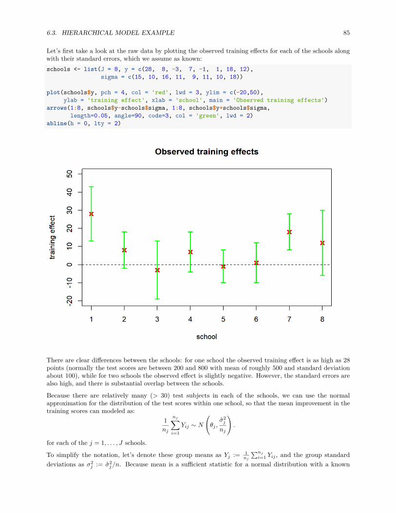
6.3. HIERARCHICAL MODEL EXAMPLE 85
Let’s first take a look at the raw data by plotting the observed training effects for each of the schools alongwith their standard errors, which we assume as known:schools <- list(J = 8, y = c(28, 8, -3, 7, -1, 1, 18, 12),
sigma = c(15, 10, 16, 11, 9, 11, 10, 18))
plot(schools$y, pch = 4, col = 'red', lwd = 3, ylim = c(-20,50),ylab = 'training effect', xlab = 'school', main = 'Observed training effects')
arrows(1:8, schools$y-schools$sigma, 1:8, schools$y+schools$sigma,length=0.05, angle=90, code=3, col = 'green', lwd = 2)
abline(h = 0, lty = 2)
There are clear differences between the schools: for one school the observed training effect is as high as 28points (normally the test scores are between 200 and 800 with mean of roughly 500 and standard deviationabout 100), while for two schools the observed effect is slightly negative. However, the standard errors arealso high, and there is substantial overlap between the schools.
Because there are relatively many (> 30) test subjects in each of the schools, we can use the normalapproximation for the distribution of the test scores within one school, so that the mean improvement in thetraining scores can modeled as:
1nj
nj∑i=1
Yij ∼ N
(θj ,
σ2j
nj
).
for each of the j = 1, . . . , J schools.
To simplify the notation, let’s denote these group means as Yj := 1nj
∑nji=1 Yij , and the group standard
deviations as σ2j := σ2
j /n. Because mean is a sufficient statistic for a normal distribution with a known
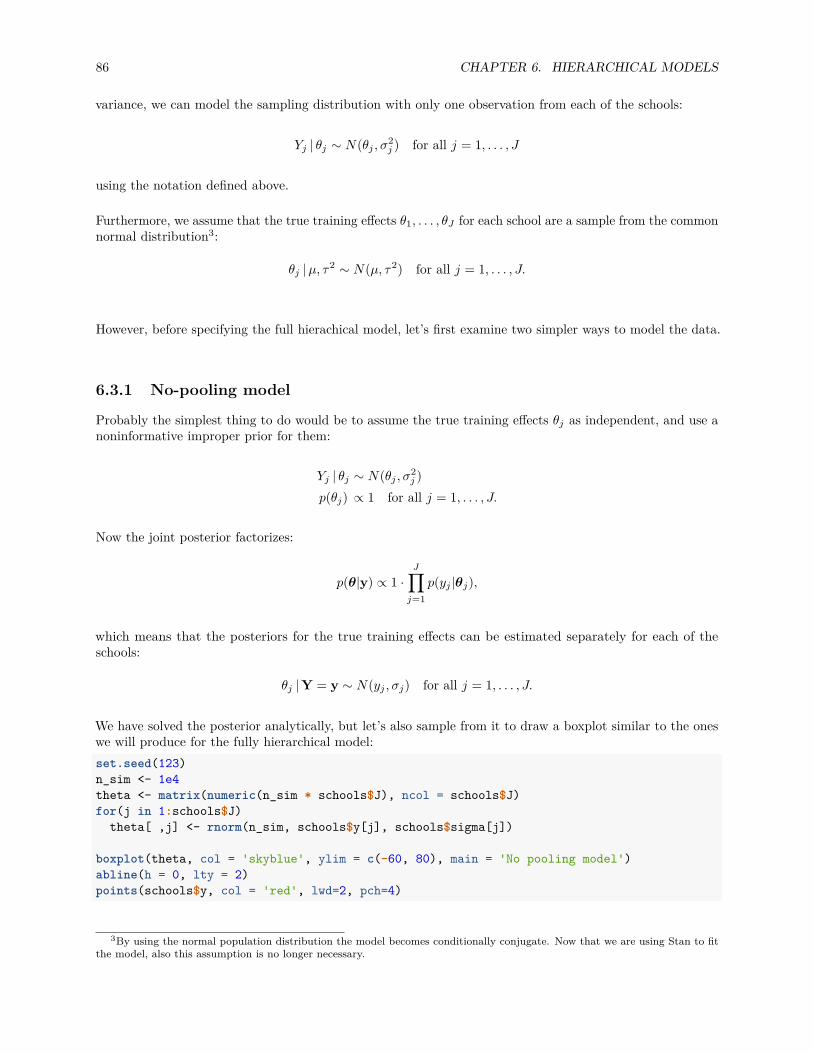
86 CHAPTER 6. HIERARCHICAL MODELS
variance, we can model the sampling distribution with only one observation from each of the schools:
Yj | θj ∼ N(θj , σ2j ) for all j = 1, . . . , J
using the notation defined above.
Furthermore, we assume that the true training effects θ1, . . . , θJ for each school are a sample from the commonnormal distribution3:
θj |µ, τ2 ∼ N(µ, τ2) for all j = 1, . . . , J.
However, before specifying the full hierachical model, let’s first examine two simpler ways to model the data.
6.3.1 No-pooling model
Probably the simplest thing to do would be to assume the true training effects θj as independent, and use anoninformative improper prior for them:
Yj | θj ∼ N(θj , σ2j )
p(θj) ∝ 1 for all j = 1, . . . , J.
Now the joint posterior factorizes:
p(θ|y) ∝ 1 ·J∏j=1
p(yj |θj),
which means that the posteriors for the true training effects can be estimated separately for each of theschools:
θj |Y = y ∼ N(yj , σj) for all j = 1, . . . , J.
We have solved the posterior analytically, but let’s also sample from it to draw a boxplot similar to the oneswe will produce for the fully hierarchical model:set.seed(123)n_sim <- 1e4theta <- matrix(numeric(n_sim * schools$J), ncol = schools$J)for(j in 1:schools$J)
theta[ ,j] <- rnorm(n_sim, schools$y[j], schools$sigma[j])
boxplot(theta, col = 'skyblue', ylim = c(-60, 80), main = 'No pooling model')abline(h = 0, lty = 2)points(schools$y, col = 'red', lwd=2, pch=4)
3By using the normal population distribution the model becomes conditionally conjugate. Now that we are using Stan to fitthe model, also this assumption is no longer necessary.
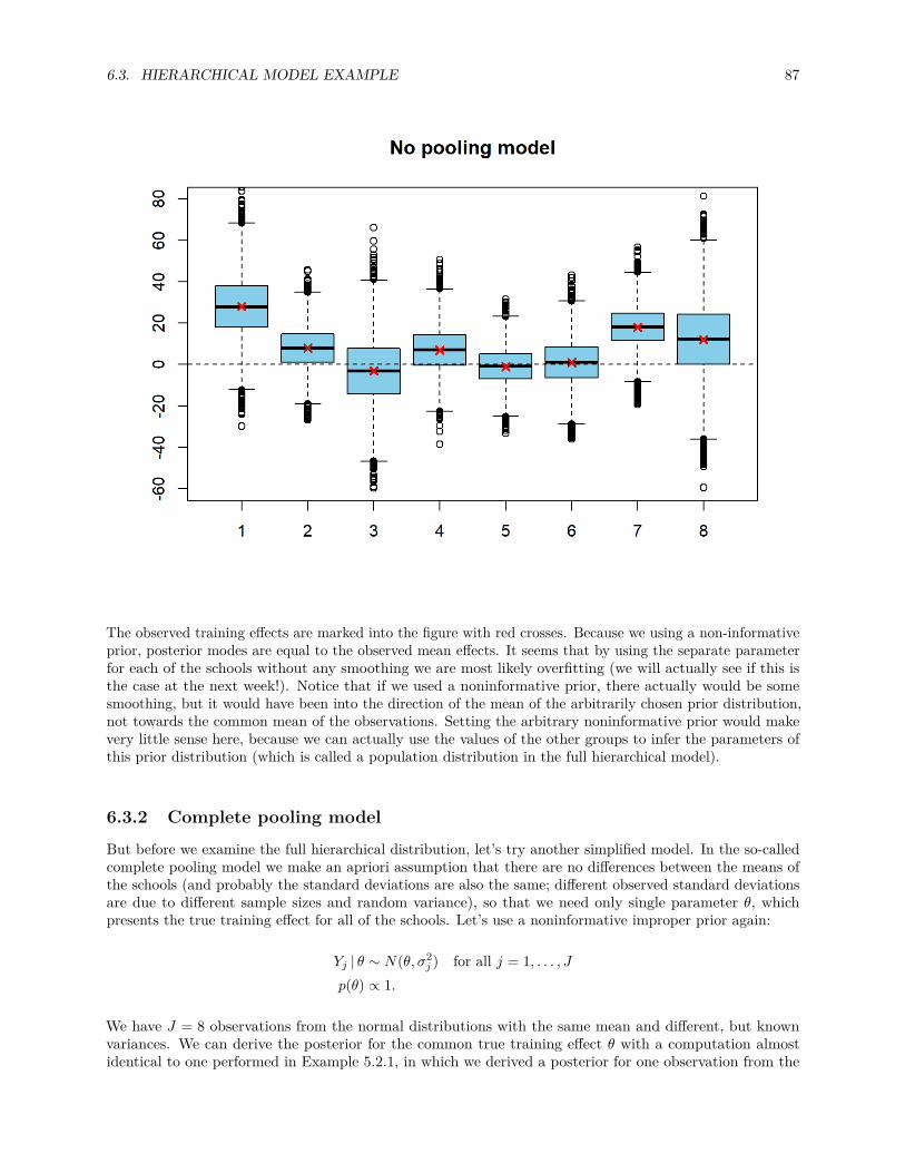
6.3. HIERARCHICAL MODEL EXAMPLE 87
The observed training effects are marked into the figure with red crosses. Because we using a non-informativeprior, posterior modes are equal to the observed mean effects. It seems that by using the separate parameterfor each of the schools without any smoothing we are most likely overfitting (we will actually see if this isthe case at the next week!). Notice that if we used a noninformative prior, there actually would be somesmoothing, but it would have been into the direction of the mean of the arbitrarily chosen prior distribution,not towards the common mean of the observations. Setting the arbitrary noninformative prior would makevery little sense here, because we can actually use the values of the other groups to infer the parameters ofthis prior distribution (which is called a population distribution in the full hierarchical model).
6.3.2 Complete pooling model
But before we examine the full hierarchical distribution, let’s try another simplified model. In the so-calledcomplete pooling model we make an apriori assumption that there are no differences between the means ofthe schools (and probably the standard deviations are also the same; different observed standard deviationsare due to different sample sizes and random variance), so that we need only single parameter θ, whichpresents the true training effect for all of the schools. Let’s use a noninformative improper prior again:
Yj | θ ∼ N(θ, σ2j ) for all j = 1, . . . , J
p(θ) ∝ 1.
We have J = 8 observations from the normal distributions with the same mean and different, but knownvariances. We can derive the posterior for the common true training effect θ with a computation almostidentical to one performed in Example 5.2.1, in which we derived a posterior for one observation from the
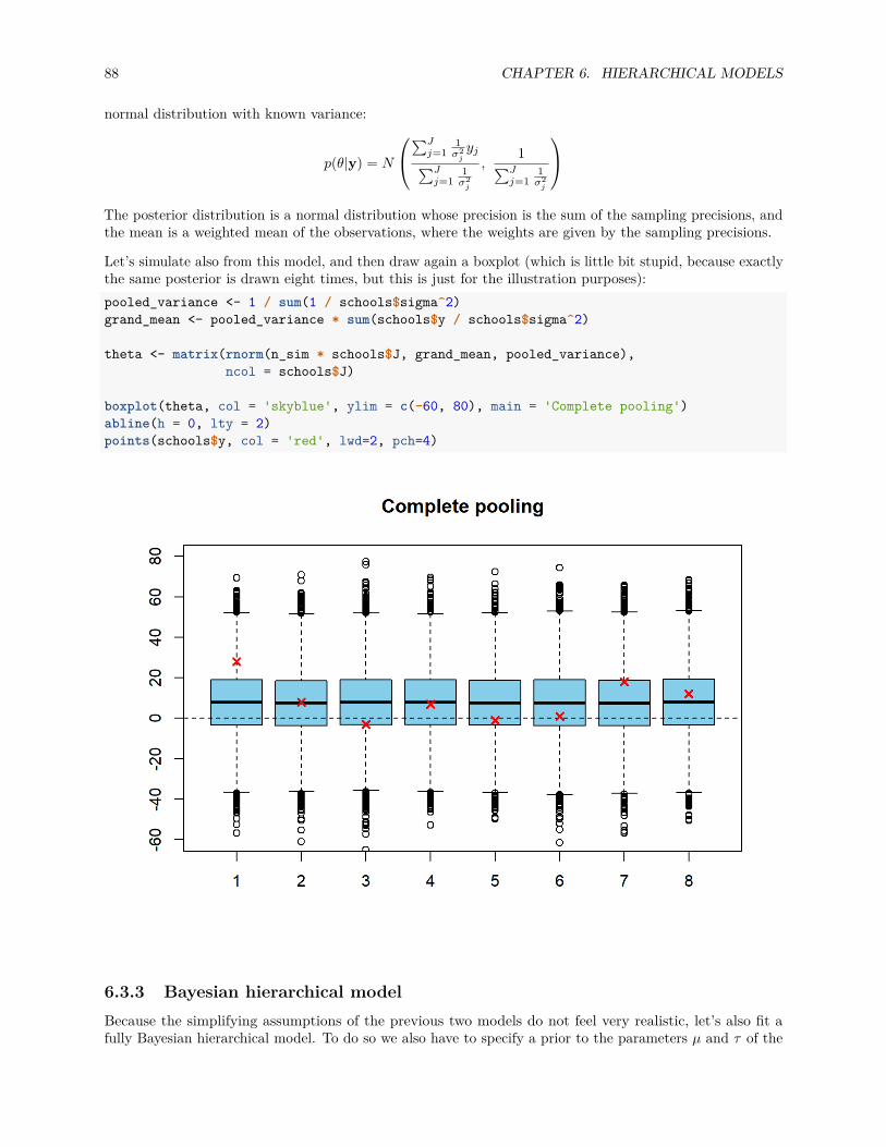
88 CHAPTER 6. HIERARCHICAL MODELS
normal distribution with known variance:
p(θ|y) = N
∑Jj=1
1σ2jyj∑J
j=11σ2j
,1∑J
j=11σ2j
The posterior distribution is a normal distribution whose precision is the sum of the sampling precisions, andthe mean is a weighted mean of the observations, where the weights are given by the sampling precisions.
Let’s simulate also from this model, and then draw again a boxplot (which is little bit stupid, because exactlythe same posterior is drawn eight times, but this is just for the illustration purposes):pooled_variance <- 1 / sum(1 / schools$sigma^2)grand_mean <- pooled_variance * sum(schools$y / schools$sigma^2)
theta <- matrix(rnorm(n_sim * schools$J, grand_mean, pooled_variance),ncol = schools$J)
boxplot(theta, col = 'skyblue', ylim = c(-60, 80), main = 'Complete pooling')abline(h = 0, lty = 2)points(schools$y, col = 'red', lwd=2, pch=4)
6.3.3 Bayesian hierarchical modelBecause the simplifying assumptions of the previous two models do not feel very realistic, let’s also fit afully Bayesian hierarchical model. To do so we also have to specify a prior to the parameters µ and τ of the
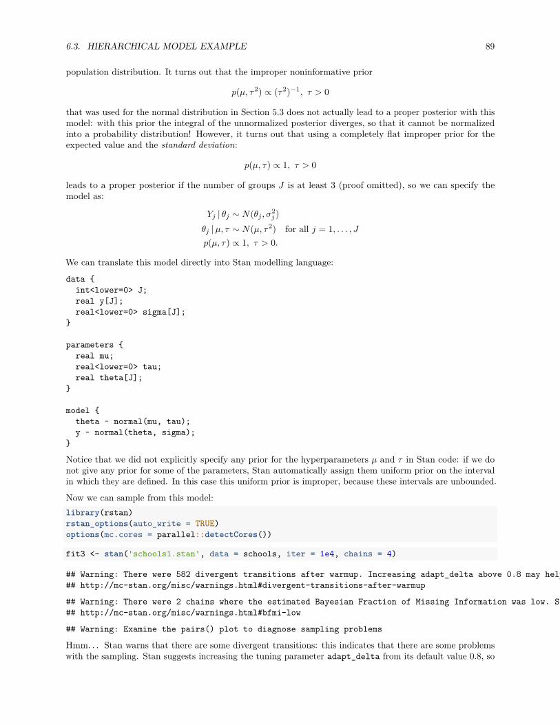
6.3. HIERARCHICAL MODEL EXAMPLE 89
population distribution. It turns out that the improper noninformative prior
p(µ, τ2) ∝ (τ2)−1, τ > 0
that was used for the normal distribution in Section 5.3 does not actually lead to a proper posterior with thismodel: with this prior the integral of the unnormalized posterior diverges, so that it cannot be normalizedinto a probability distribution! However, it turns out that using a completely flat improper prior for theexpected value and the standard deviation:
p(µ, τ) ∝ 1, τ > 0
leads to a proper posterior if the number of groups J is at least 3 (proof omitted), so we can specify themodel as:
Yj | θj ∼ N(θj , σ2j )
θj |µ, τ ∼ N(µ, τ2) for all j = 1, . . . , Jp(µ, τ) ∝ 1, τ > 0.
We can translate this model directly into Stan modelling language:
data int<lower=0> J;real y[J];real<lower=0> sigma[J];
parameters real mu;real<lower=0> tau;real theta[J];
model theta ~ normal(mu, tau);y ~ normal(theta, sigma);
Notice that we did not explicitly specify any prior for the hyperparameters µ and τ in Stan code: if we donot give any prior for some of the parameters, Stan automatically assign them uniform prior on the intervalin which they are defined. In this case this uniform prior is improper, because these intervals are unbounded.
Now we can sample from this model:library(rstan)rstan_options(auto_write = TRUE)options(mc.cores = parallel::detectCores())
fit3 <- stan('schools1.stan', data = schools, iter = 1e4, chains = 4)
## Warning: There were 582 divergent transitions after warmup. Increasing adapt_delta above 0.8 may help. See## http://mc-stan.org/misc/warnings.html#divergent-transitions-after-warmup
## Warning: There were 2 chains where the estimated Bayesian Fraction of Missing Information was low. See## http://mc-stan.org/misc/warnings.html#bfmi-low
## Warning: Examine the pairs() plot to diagnose sampling problems
Hmm. . . Stan warns that there are some divergent transitions: this indicates that there are some problemswith the sampling. Stan suggests increasing the tuning parameter adapt_delta from its default value 0.8, so
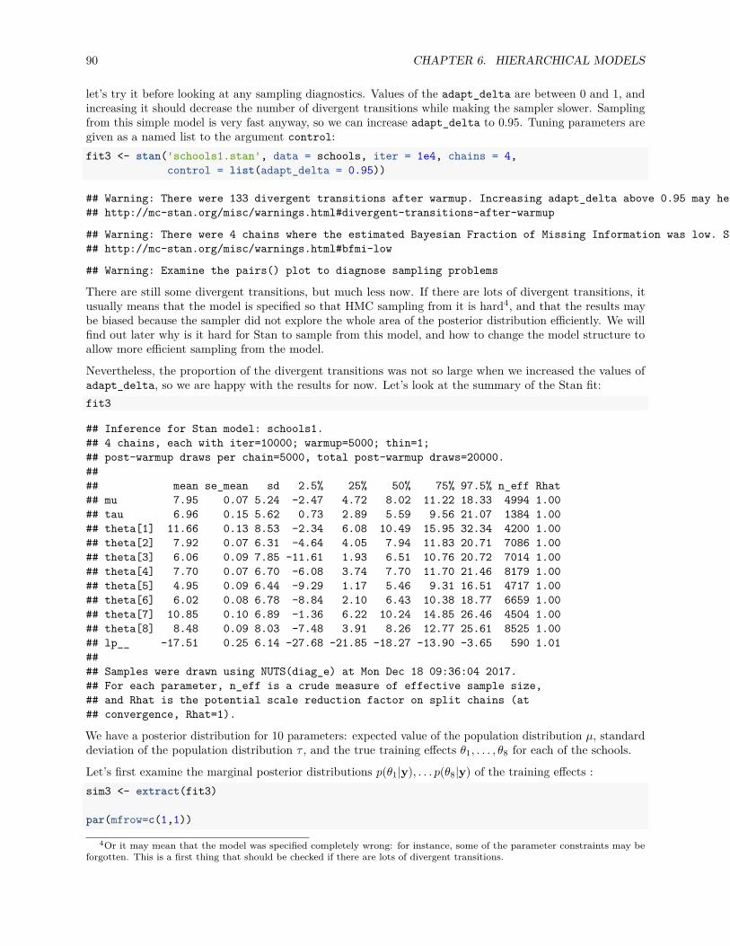
90 CHAPTER 6. HIERARCHICAL MODELS
let’s try it before looking at any sampling diagnostics. Values of the adapt_delta are between 0 and 1, andincreasing it should decrease the number of divergent transitions while making the sampler slower. Samplingfrom this simple model is very fast anyway, so we can increase adapt_delta to 0.95. Tuning parameters aregiven as a named list to the argument control:fit3 <- stan('schools1.stan', data = schools, iter = 1e4, chains = 4,
control = list(adapt_delta = 0.95))
## Warning: There were 133 divergent transitions after warmup. Increasing adapt_delta above 0.95 may help. See## http://mc-stan.org/misc/warnings.html#divergent-transitions-after-warmup
## Warning: There were 4 chains where the estimated Bayesian Fraction of Missing Information was low. See## http://mc-stan.org/misc/warnings.html#bfmi-low
## Warning: Examine the pairs() plot to diagnose sampling problems
There are still some divergent transitions, but much less now. If there are lots of divergent transitions, itusually means that the model is specified so that HMC sampling from it is hard4, and that the results maybe biased because the sampler did not explore the whole area of the posterior distribution efficiently. We willfind out later why is it hard for Stan to sample from this model, and how to change the model structure toallow more efficient sampling from the model.
Nevertheless, the proportion of the divergent transitions was not so large when we increased the values ofadapt_delta, so we are happy with the results for now. Let’s look at the summary of the Stan fit:fit3
## Inference for Stan model: schools1.## 4 chains, each with iter=10000; warmup=5000; thin=1;## post-warmup draws per chain=5000, total post-warmup draws=20000.#### mean se_mean sd 2.5% 25% 50% 75% 97.5% n_eff Rhat## mu 7.95 0.07 5.24 -2.47 4.72 8.02 11.22 18.33 4994 1.00## tau 6.96 0.15 5.62 0.73 2.89 5.59 9.56 21.07 1384 1.00## theta[1] 11.66 0.13 8.53 -2.34 6.08 10.49 15.95 32.34 4200 1.00## theta[2] 7.92 0.07 6.31 -4.64 4.05 7.94 11.83 20.71 7086 1.00## theta[3] 6.06 0.09 7.85 -11.61 1.93 6.51 10.76 20.72 7014 1.00## theta[4] 7.70 0.07 6.70 -6.08 3.74 7.70 11.70 21.46 8179 1.00## theta[5] 4.95 0.09 6.44 -9.29 1.17 5.46 9.31 16.51 4717 1.00## theta[6] 6.02 0.08 6.78 -8.84 2.10 6.43 10.38 18.77 6659 1.00## theta[7] 10.85 0.10 6.89 -1.36 6.22 10.24 14.85 26.46 4504 1.00## theta[8] 8.48 0.09 8.03 -7.48 3.91 8.26 12.77 25.61 8525 1.00## lp__ -17.51 0.25 6.14 -27.68 -21.85 -18.27 -13.90 -3.65 590 1.01#### Samples were drawn using NUTS(diag_e) at Mon Dec 18 09:36:04 2017.## For each parameter, n_eff is a crude measure of effective sample size,## and Rhat is the potential scale reduction factor on split chains (at## convergence, Rhat=1).
We have a posterior distribution for 10 parameters: expected value of the population distribution µ, standarddeviation of the population distribution τ , and the true training effects θ1, . . . , θ8 for each of the schools.
Let’s first examine the marginal posterior distributions p(θ1|y), . . . p(θ8|y) of the training effects :sim3 <- extract(fit3)
par(mfrow=c(1,1))
4Or it may mean that the model was specified completely wrong: for instance, some of the parameter constraints may beforgotten. This is a first thing that should be checked if there are lots of divergent transitions.
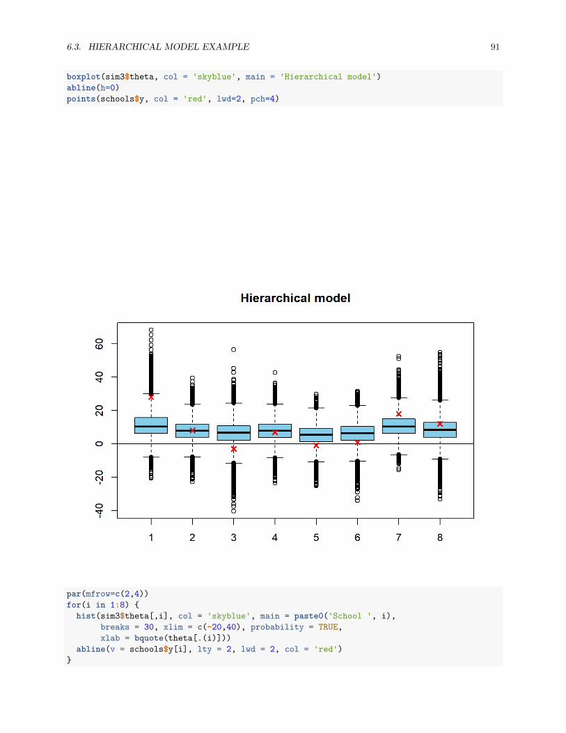
6.3. HIERARCHICAL MODEL EXAMPLE 91
boxplot(sim3$theta, col = 'skyblue', main = 'Hierarchical model')abline(h=0)points(schools$y, col = 'red', lwd=2, pch=4)
par(mfrow=c(2,4))for(i in 1:8)
hist(sim3$theta[,i], col = 'skyblue', main = paste0('School ', i),breaks = 30, xlim = c(-20,40), probability = TRUE,xlab = bquote(theta[.(i)]))
abline(v = schools$y[i], lty = 2, lwd = 2, col = 'red')
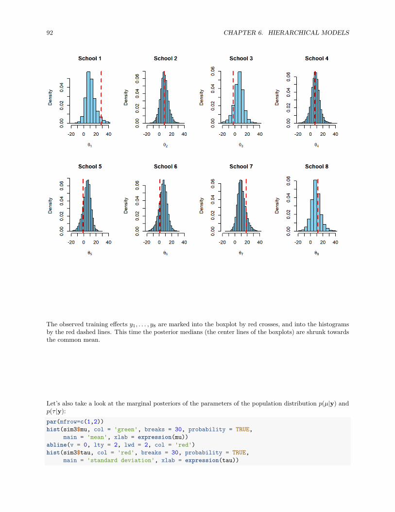
92 CHAPTER 6. HIERARCHICAL MODELS
The observed training effects y1, . . . , y8 are marked into the boxplot by red crosses, and into the histogramsby the red dashed lines. This time the posterior medians (the center lines of the boxplots) are shrunk towardsthe common mean.
Let’s also take a look at the marginal posteriors of the parameters of the population distribution p(µ|y) andp(τ |y):par(mfrow=c(1,2))hist(sim3$mu, col = 'green', breaks = 30, probability = TRUE,
main = 'mean', xlab = expression(mu))abline(v = 0, lty = 2, lwd = 2, col = 'red')hist(sim3$tau, col = 'red', breaks = 30, probability = TRUE,
main = 'standard deviation', xlab = expression(tau))
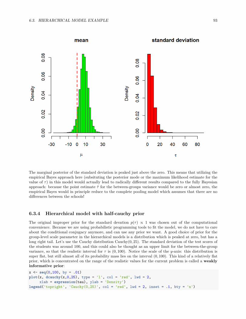
6.3. HIERARCHICAL MODEL EXAMPLE 93
The marginal posterior of the standard deviation is peaked just above the zero. This means that utilizing theempirical Bayes approach here (subsituting the posterior mode or the maximum likelihood estimate for thevalue of τ) in this model would actually lead to radically different results compared to the fully Bayesianapproach: because the point estimate τ for the between-groups variance would be zero or almost zero, theempirical Bayes would in principle reduce to the complete pooling model which assumes that there are nodifferences between the schools!
6.3.4 Hierarchical model with half-cauchy prior
The original improper prior for the standard devation p(τ) ∝ 1 was chosen out of the computationalconvenience. Because we are using probabilistic programming tools to fit the model, we do not have to careabout the conditional conjugacy anymore, and can use any prior we want. A good choice of prior for thegroup-level scale parameter in the hierarchical models is a distribution which is peaked at zero, but has along right tail. Let’s use the Cauchy distribution Cauchy(0, 25). The standard deviation of the test scores ofthe students was around 100, and this could also be thought as an upper limit for the between-the-groupvariance, so that the realistic interval for τ is (0, 100). Notice the scale of the y-axis: this distribution issuper flat, but still almost all of its probability mass lies on the interval (0, 100). This kind of a relatively flatprior, which is concentrated on the range of the realistic values for the current problem is called a weaklyinformative prior:x <- seq(0,100, by = .01)plot(x, dcauchy(x,0,25), type = 'l', col = 'red', lwd = 2,
xlab = expression(tau), ylab = 'Density')legend('topright', 'Cauchy(0,25)', col = 'red', lwd = 2, inset = .1, bty = 'n')
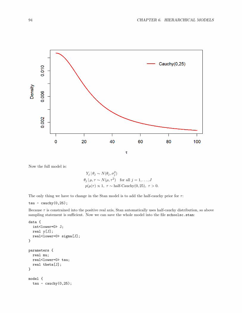
94 CHAPTER 6. HIERARCHICAL MODELS
Now the full model is:
Yj | θj ∼ N(θj , σ2j )
θj |µ, τ ∼ N(µ, τ2) for all j = 1, . . . , Jp(µ|τ) ∝ 1, τ ∼ half-Cauchy(0, 25), τ > 0.
The only thing we have to change in the Stan model is to add the half-cauchy prior for τ :
tau ~ cauchy(0,25);
Because τ is constrained into the positive real axis, Stan automatically uses half-cauchy distribution, so abovesampling statement is sufficient. Now we can save the whole model into the file schoolsc.stan:
data int<lower=0> J;real y[J];real<lower=0> sigma[J];
parameters real mu;real<lower=0> tau;real theta[J];
model tau ~ cauchy(0,25);
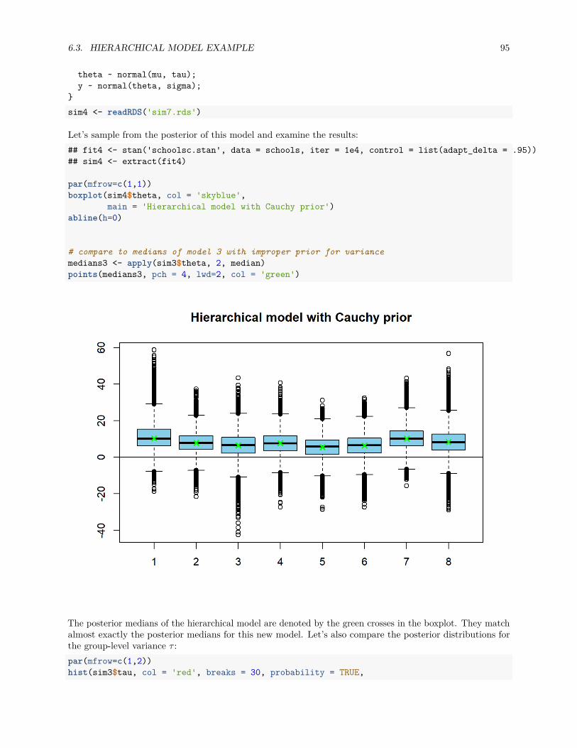
6.3. HIERARCHICAL MODEL EXAMPLE 95
theta ~ normal(mu, tau);y ~ normal(theta, sigma);
sim4 <- readRDS('sim7.rds')
Let’s sample from the posterior of this model and examine the results:## fit4 <- stan('schoolsc.stan', data = schools, iter = 1e4, control = list(adapt_delta = .95))## sim4 <- extract(fit4)
par(mfrow=c(1,1))boxplot(sim4$theta, col = 'skyblue',
main = 'Hierarchical model with Cauchy prior')abline(h=0)
# compare to medians of model 3 with improper prior for variancemedians3 <- apply(sim3$theta, 2, median)points(medians3, pch = 4, lwd=2, col = 'green')
The posterior medians of the hierarchical model are denoted by the green crosses in the boxplot. They matchalmost exactly the posterior medians for this new model. Let’s also compare the posterior distributions forthe group-level variance τ :par(mfrow=c(1,2))hist(sim3$tau, col = 'red', breaks = 30, probability = TRUE,
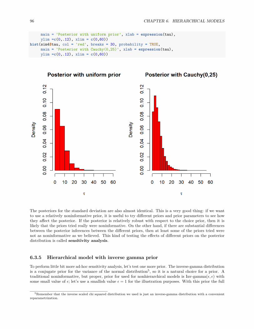
96 CHAPTER 6. HIERARCHICAL MODELS
main = 'Posterior with uniform prior', xlab = expression(tau),ylim =c(0,.12), xlim = c(0,60))
hist(sim4$tau, col = 'red', breaks = 30, probability = TRUE,main = 'Posterior with Cauchy(0,25)', xlab = expression(tau),ylim =c(0,.12), xlim = c(0,60))
The posteriors for the standard deviation are also almost identical. This is a very good thing: if we wantto use a relatively noninformative prior, it is useful to try different priors and prior parameters to see howthey affect the posterior. If the posterior is relatively robust with respect to the choice prior, then it islikely that the priors tried really were noninformative. On the other hand, if there are substantial differencesbetween the posterior inferences between the different priors, then at least some of the priors tried werenot as noninformative as we believed. This kind of testing the effects of different priors on the posteriordistribution is called sensitivity analysis.
6.3.5 Hierarchical model with inverse gamma prior
To perform little bit more ad-hoc sensitivity analysis, let’s test one more prior. The inverse-gamma distributionis a conjugate prior for the variance of the normal distribution5, so it is a natural choice for a prior. Atraditional noninformative, but proper, prior for used for nonhierarchical models is Inv-gamma(ε, ε) withsome small value of ε; let’s use a smallish value ε = 1 for the illustration purposes. With this prior the full
5Remember that the inverse scaled chi squared distribution we used is just an inverse-gamma distribution with a convenientreparametrization.
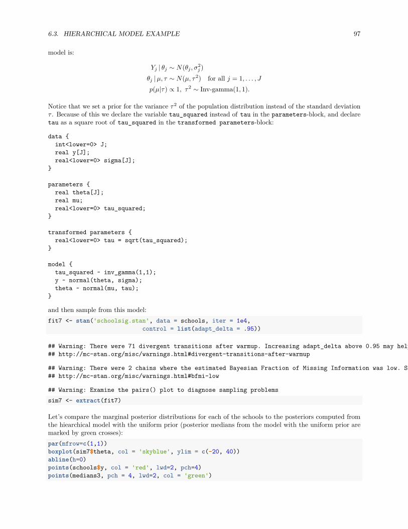
6.3. HIERARCHICAL MODEL EXAMPLE 97
model is:
Yj | θj ∼ N(θj , σ2j )
θj |µ, τ ∼ N(µ, τ2) for all j = 1, . . . , Jp(µ|τ) ∝ 1, τ2 ∼ Inv-gamma(1, 1).
Notice that we set a prior for the variance τ2 of the population distribution instead of the standard deviationτ . Because of this we declare the variable tau_squared instead of tau in the parameters-block, and declaretau as a square root of tau_squared in the transformed parameters-block:
data int<lower=0> J;real y[J];real<lower=0> sigma[J];
parameters real theta[J];real mu;real<lower=0> tau_squared;
transformed parameters real<lower=0> tau = sqrt(tau_squared);
model tau_squared ~ inv_gamma(1,1);y ~ normal(theta, sigma);theta ~ normal(mu, tau);
and then sample from this model:fit7 <- stan('schoolsig.stan', data = schools, iter = 1e4,
control = list(adapt_delta = .95))
## Warning: There were 71 divergent transitions after warmup. Increasing adapt_delta above 0.95 may help. See## http://mc-stan.org/misc/warnings.html#divergent-transitions-after-warmup
## Warning: There were 2 chains where the estimated Bayesian Fraction of Missing Information was low. See## http://mc-stan.org/misc/warnings.html#bfmi-low
## Warning: Examine the pairs() plot to diagnose sampling problemssim7 <- extract(fit7)
Let’s compare the marginal posterior distributions for each of the schools to the posteriors computed fromthe hiearchical model with the uniform prior (posterior medians from the model with the uniform prior aremarked by green crosses):par(mfrow=c(1,1))boxplot(sim7$theta, col = 'skyblue', ylim = c(-20, 40))abline(h=0)points(schools$y, col = 'red', lwd=2, pch=4)points(medians3, pch = 4, lwd=2, col = 'green')
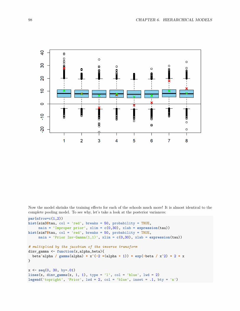
98 CHAPTER 6. HIERARCHICAL MODELS
Now the model shrinks the training effects for each of the schools much more! It is almost identical to thecomplete pooling model. To see why, let’s take a look at the posterior variances:par(mfrow=c(1,2))hist(sim3$tau, col = 'red', breaks = 50, probability = TRUE,
main = 'Improper prior', xlim = c(0,30), xlab = expression(tau))hist(sim7$tau, col = 'red', breaks = 50, probability = TRUE,
main = 'Prior Inv-Gamma(1,1)', xlim = c(0,30), xlab = expression(tau))
# multiplied by the jacobian of the inverse transformdinv_gamma <- function(x,alpha,beta)
beta^alpha / gamma(alpha) * x^(-2 *(alpha + 1)) * exp(-beta / x^2) * 2 * x
x <- seq(0, 30, by=.01)lines(x, dinv_gamma(x, 1, 1), type = 'l', col = 'blue', lwd = 2)legend('topright', 'Prior', lwd = 2, col = 'blue', inset = .1, bty = 'n')
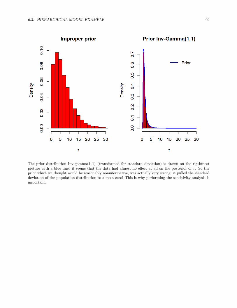
6.3. HIERARCHICAL MODEL EXAMPLE 99
The prior distribution Inv-gamma(1, 1) (transformed for standard deviation) is drawn on the rigthmostpicture with a blue line: it seems that the data had almost no effect at all on the posterior of τ . So theprior which we thought would be reasonably noninformative, was actually very strong: it pulled the standarddeviation of the population distribution to almost zero! This is why performing the sensitivity analysis isimportant.

100 CHAPTER 6. HIERARCHICAL MODELS
Chapter 7
Linear model
So far on this course we have examined models with no predictors. However, usually the modeling situationis that have the observations Y1, . . . , Yn, often called response variable or output variable, and for eachobservation Yi we have the vector of predictors xi = (xi1, . . . , xik), which we use to predict its value.
We are interested in values of the response variable given the predictors, so they we can think the values ofthe predictors as constants, i.e. we do not have to set any prior for the them.
Liner models and generalized linear model are one of the most important tools of applied statistican. Inprinciple the inference does not differ from the computations we have done earlier on this course. We havealready examined the posterior inference for the normal distribution, on which the linear models are basedon. However, usually on linear models we have multiple predictors: this means that the posterior for theregression coefficients is a multinormal distribution. This complicates the things a little bit, but the principlestays the same.
We can collect the values of the predicted variable Y = (Y1, . . . , Yn) into the n× 1-matrix
Y =
Y1...Yn
,and the values of the predictors into the n× k-matrix
X =
x11 . . . x1k...
...xn1 . . . xnk
,so that we can use a convenient matrix notation for the linear model. Usually we also want to add a constantterm into the model. This can be incorporated into the vector notation by setting the first column of thematrix of the predictors into the vector of ones: (x11, . . . , xn1) = 1n. The regression coefficients can bewritten into the k × 1-matrix
β =
β1...βk
,where β1 is the intercept of the model (if the constant term is used). Now our model is of the form
Y = X · β. (7.1)
101
102 CHAPTER 7. LINEAR MODEL
7.1 Classical linear modelIn the classical linear model, also known as ordinary least squares regression, it is assumed that theresponse variables are independent, and follow normal distributions given the values of the predictors, andthat the expected values of these normal distributions are linear combinations of the regression coefficients β:
E[Yi |β,xi] = xTi β = xi1β1 + · · ·+ xikβk,
and that these normal distributions have a same variance σ2. In the Bayesian setting the noninformativeprior for the parameter vector is p(β, σ2) ∝ (σ2)−1. This means that the model can be written as
Yi |β, σ2 ∼ N(xTi β, σ2) for all i = 1, . . . , n,
p(β, σ2) ∝ 1σ2 ,
or more compactly using the matrix notation introduced above as:
Y ∼ N(Xβ, σ2I)
p(β, σ2) ∝ 1σ2 .
7.2 Posterior for classical linear regressionWith derivations similar to the ones done in Section 5.3 we can show that the conditional posterior distributionp(β|σ2,y) of the regression coefficients given the variance is a k-dimensional multinormal distribution
β |y, σ2 ∼ N(β, Vβσ2),
whereβ = (XTX)−1XTy,
andVβ = (XTX)−1.
The marginal posterior distribution for the variance σ2 is an inverted chi-squared distribution with degrees offreedom n− k:
σ2|y ∼ χ−2n−k(s2),
wheres2 = 1
n− k(y−Xβ)T (y−Xβ).
We can observe that when the noninformative prior is used, the results are again quite close to the results ofthe frequentist statistical inference for the linear model.
7.3 Posterior distribution of β
We now solve the posterior distribution for β, given the parameter σ2 and our data X:
p(β|y,X, σ2) ∝ p(y|β,X, σ2)p(β)
Let us continue with a noninformative prior p(β) ∝ 1. Note that now we handle σ as a fixed variable. Withthis choice of prior, it is sufficient to focus only on the conditional distribution of y and recognize a targetdistribution for β when assuming that y, X and σ2 are fixed. We also notice, that we end up having thesame posterior for β as with the assumptions in 7.2. Let us start with the likelihood,
7.4. FULL MODEL WITH THE PREDICTORS 103
p(y|β,X, σ2) ∝ σ−n exp− 12σ (y−Xβ)T (y−Xβ)
= σ−n exp− 12σ (yTy− 2βXTy + βTXTXβ)
∝ σ−n exp− 12σ (−2βXTy + βTXTXβ),
where the equality was achieved by remembering the matrix transpose rule1. As per usual, our current task isto manipulate the expression to a form where we recognize a familiar kernel. The current form would suggesta multivariate normal density – let’s aim for that and try our luck by completing the squares. We notice that
−2βXTy = −2βXTX(XTX)−1XTy,
and furthermore, let us add and subtract a constant
c = ((XTX)−1XTy)TXTX((XTX)−1XTy)
within the exponent. Now, inside the exponent, we have (notice that the constant c does not depend on β)
c− 2βXTX(XTX)−1XTy + βTXTXβ − c∝((XTX)−1XTy)TXTX((XTX)−1XTy)− 2βXTX(XTX)−1XTy + βTXTXβ=(β − (XTX)−1XTy)TXTX(β − (XTX)−1XTy).
Now let’s return the manipulated expression inside the exponential function:
p(β|y,X, σ2) ∝ σ−n exp− 12σ (β − (XTX)−1XTy)TXTX(β − (XTX)−1XTy),
and this expression can be recognized as a multivariate normal density. Thus
β|y,X, σ2 ∼ N((XTX)−1XTy, (XTX)−1σ2).
Furthermore, we could analyse a model where σ2 is assumed to be random with some prior density, and witha flat uninformative prior we would end up having the same distribution as in 7.2.
7.4 Full model with the predictorsAbove we considered the predictors X to be constant, that is, we considered the conditional model p(Y|X, σ2).Let us now extend the model further to assume that X follows a likelihood density p(X|φ) and furthermore,let us assume that the two parameters σ2 and φ are independent so that their joint prior density can becalculated as
p(σ2, φ) = p(σ2)p(φ).
Furthermore, under these assumptions their joint posterior can be calculated as
1Remember that for some matrices A and B we have (AB)T = ATBT .
104 CHAPTER 7. LINEAR MODEL
p(σ2, φ|X,Y) ∝ p(φ|X,Y, σ2)p(σ2|X,Y)= p(φ|X,Y)p(σ2|X,Y)
= p(Y|φ,X)p(φ|X)p(Y|X) p(σ2|X,Y)
= p(φ|X)p(σ2|X,Y),
where the last equality comes from the assumption that the predicted variable Y is conditionally independentwith the parameter φ, given our predictor X.
This means that if we assume the prior independence p(σ2, φ) = p(σ2)p(φ) gives us the chance of analysingthe
p(σ2|X,Y) ∝ p(σ2)p(Y|X, σ2)
separately from the density p(φ|X) with no loss of information. Furthermore, we could recognize the nowseparate marginal posteriors and complete the inference for both posterior distributions, respectively.
Chapter 8
Hypothesis testing and Bayes factor
To close this course and these lecture notes, we venture back to the fundamentals of statistical inference:hypothesis testing. Hypothesis testing is a classical part of statistical inference and in this chapter, we focuson the Bayesian approach to hypothesis testing, which is based on Bayes factors. Some preliminaries offrequentist hypothesis testing will help to formulate the basic concepts regarding hypotheses, but is notnecessary. Let us start with the basics and define the hypotheses regarding the parameter space precisely asin Young and Smith (2005): in this chapter we consider a parameter space Θ, and furthermore we considerhypotheses of the form
H0 : θ ∈ Θ0 vs. H1 : θ ∈ Θ1,
where Θ0 and Θ1 are two disjoint subsets of Θ, and in our case we limit ourselves to the special case whereΘ0 ∪ Θ1 = Θ. Furthermore, if a hypothesis contains a single element of Θ, we say that it is a simplehypothesis. Otherwise the hypothesis is called a composite. We assign probabilities pi for each Θi, i = 0, 1,and furthermore assume that both probabilities p0 and p1 are nonnegative. Since we assumed that the Θ0and Θ1 divide the parameter space Θ, it is natural to conclude that p0 + p1 = 1.
In the frequentist hypothesis testing, we can not really assign any probabilities into the hypotheses: forexample, we can not give a clear probability for the hypotesis H0 to be true. Instead, in a very frequentistsense of a world, we assign a p-value to the data, where the p-value gives the probability of ”obtaining moreextreme data than we observed, given that we could repeat the experiment infinitely and given that the nullhypothesis H0 holds". However, in the Bayesian framework we can actually denote such probability to eachhypothesis Hi.
Abusing the Bayes theorem, we find that the probability for the null hypothesis H0, given the data X with adensity f(x), is
P (H0 is true|X = x) = P (θ ∈ Θ0|X = x) = p0f(x|θ ∈ Θ0)p0f(x|θ ∈ Θ0) + p1f(x|θ ∈ Θ1) .
A similar conditional probability could be calculated for H1. In particular, we can obtain a ratio
P (H0 is true|X = x)P (H1 is true|X = x) = p0
p1
f(x|θ ∈ Θ0)f(x|θ ∈ Θ1) ,
where we denote the ratio
p0
p1
105
106 CHAPTER 8. HYPOTHESIS TESTING AND BAYES FACTOR
as prior odds in favour of H0 over H1, and furthermore denote the ratio
B := f(x|θ ∈ Θ0)f(x|θ ∈ Θ1)
as the Bayes factor. In a similar manner, the ratio of the posterior probabilities is called posterior odds.
The prior and the posterior odds can be thought as the degrees of belief regarding H0, respectively beforeand after assessing the data. The Bayes factor measures how much the data changes the prior beliefs (odds),or in other words, what is the strength of the data in the posterior probabilities. Furthermore, if B > 1, wecan conclude that the data gave some support for the hypothesis H0.
In other words, the Bayes factor provides us a scale of evidence in favour of one hypothesis against the other.Note that, however, the scale is from zero to infinity, which may not be as easily comprehensible as a simpleprobability scale (which is defined on [0, 1]).
From the point of decision theory, the Bayes rule will be used as a measurement for belief regarding thehypothesis H0 and furthermore, we will reject the H0 if B < k for some fixed k ∈ [0,∞], and otherwise acceptthe null hypothesis H1. Jeffreys argued in 1939 (in his book Theory of Probability), that whenever B > 1,the data supports the H0 and if B < 0.1, then the data is a strong evidence against the H0, and furthermore,if B < 0.01, then the data is a decisive evidence against the null hypothesis. In a sense, the mechanic ofrejecting or accepting the hypotheses is precisely the same as in the classical set-up.
However, to depart from the classical hypothesis testing, the argument is that the Bayes factor is a meaningfulmeasurement in its own right, without having the full arsenal of significance levels and such to guide us.
8.1 Bayes factors for point hypothesisWhen having a point hypothesis, the calculation of the Bayes factor is fairly straight-forward. With a pointhypothesis we have a simple H0 : θ = θ0, where θ0 ∈ Θ0, against another point hypothesis H1 : θ = θ1, wheresimilarly θ1 ∈ Θ1. Due to our assumptions, we have positive probabilities for both values, and now theposterior odds are
P (θ = θ0|X = x)P (θ = θ1|X = x) = P (θ = θ0)
P (θ = θ1)f(x|θ = θ0)f(x|θ = θ1) .
Now we notice that the likelihood ratio is indeed the Bayes factor, and thus the Bayes factor does not dependon the prior. Furthermore, we notice that the equation holds (and there is no need to use the ∝ sign) sincethe division cancels out the normalizing constants. Now the Bayes factor can be calculated as
B = f(x|θ = θ0)f(x|θ = θ1) = P (θ = θ0|X = x)
P (θ = θ1|X = x)P (θ = θ1)P (θ = θ0) .
8.2 Bayes factors for composite hypothesisNow assume that the hypotheses are composite. In order to calculate the Bayes factors, we need to know thecomplete prior distribution for θ. Now suppose that θ has a prior distribution of f0(θ) under H0 : θ ∈ Θ0 orf1(θ) under H1 : θ ∈ Θ1. Now the Bayes factor can be calculated as
B =∫
Θ0f(x|θ)f0(θ) dθ∫
Θ1f(x|θ)f1(θ) dθ
.
In the special case where we have a simple H0 and a composite H1 we can write the Bayes factor as
8.3. EXAMPLE HYPOTHESES REGARDING POPULATION PREVALENCE 107
B = f(x|θ = θ0)∫Θ1f(x|θ)f1(θ) dθ
.
We are able to generalize the argument to a model choice problem where we have two competing models.Note that we actually do not require the same parametrization for θ under the hypotheses. Now assumethat we have two candidate parametric models, M1 and M2 regarding our data X with respective parametervectors θ1 and θ2. Denote the prior densities in these models as pi(θi) for i = 1, 2, and furthermore calculatethe marginal distribution of X as
f(x|Mi) =∫
Θif(x|θi,Mi)pi(θi) dθi
for both i = 1, 2. Now the Bayes factor can be calculated as a ratio of these:
B = f(x|M1)f(x|M2)
Now we have a similar problem than in the hypothesis testing: we are looking whether the data supports themodel M1 or does it prove some evidence against it. Again, note that the parameter dimensions on θi mightbe different – the meaning behind the Bayes factor stays the same even though the calculation might getcomplicated.
8.3 Example hypotheses regarding population prevalenceThis example is taken from Jukka Ranta’s 2015 lecture notes, and is a fairly straight-forward example incomputing the Bayes factor.
Consider a case where you are interested in a population prevalence r ∈ [0, 1] regarding a contamination.You are required to test whether the poplation prevalence r < 0.5. Your knowledge of the population is a bitshy, so you are using an noninformative uniform prior for the prevalence. In addition, your boss tells you toreject the hypothesis only if the Bayes factor is below 0.1.
The likelihood distribution is X ∼ Bin(N, r), and we notice that our sufficient set of data is X = 2 andN = 3. In other words, two of the three in our sample turned out to be contamined.
Set the null hypothesis H0 : r < 0.5 and H1 : r ≥ 0.5. From previous examples, you remember that withUniform prior and Binomial likelihood you have a posterior of Beta(X + 1, N −X + 1).
Now the prior probability for the H0 is
P (H0) = P (r < 0.5) = 0.5,
and furthermore we can calculate the posterior probability as
P (H0|X,N) = P (r < 0.5|X,N) =∫ .5
0Beta(r|X + 1, N −X + 1) dr = 0.3125.
Now for the H1 we notice that P (H1) = 1− P (H0) = 0.5, and similarly P (H1|X,N) = 1− P (H0|X,N) =0.6875. The prior odds are
P (r < 0.5)P (r ≥ 0.5) = 1,

108 CHAPTER 8. HYPOTHESIS TESTING AND BAYES FACTOR
and the posterior odds are
P (r < 0.5|X,N)P (r ≥ 0.5|X,N)
0.31250.6875 = 0.4545.
We notice that the posterior odds became smaller than the prior odds, which suggest that the data providedsome evidence against the H0. Furthermore, since the prior odds equal one, we gather that
B = 0.4545
and since 0.4545 > 0.1, we do not reject the null hypothesis H0 and instead wait for our boss to give us thepermission to gather more data. If we had the same success rate with larger sample size, the Bayes factorwould have decreased sharply and we would have had eventually reject the hypothesis that under half of thepopulation was contamined.
Bibliography
Allaire, J., Xie, Y., McPherson, J., Luraschi, J., Ushey, K., Atkins, A., Wickham, H., Cheng, J., Chang, W.,and Iannone, R. (2018). rmarkdown: Dynamic Documents for R. R package version 1.11.
Bernardo, J. and Smith, A. (1994). Bayesian Theory. Wiley Series in Probability & Statistics. Wiley.
Bernardo, J. M. (1996). The concept of exchangeability and its applications. Far East Journal of MathematicalSciences, 4:111–122.
Gelman, A., Carlin, J., Stern, H., Dunson, D., Vehtari, A., and Rubin, D. (2013). Bayesian Data Analysis,Third Edition. Chapman & Hall/CRC Texts in Statistical Science. Taylor & Francis.
Goodrich, B., Gelman, A., Carpenter, B., Hoffman, M., Lee, D., Betancourt, M., Brubaker, M., Guo, J.,Li, P., Riddell, A., Inacio, M., Morris, M., Arnold, J., Goedman, R., Lau, B., Trangucci, R., Gabry, J.,Kucukelbir, A., Grant, R., Tran, D., Malecki, M., and Gao, Y. (2019). StanHeaders: C++ Header Filesfor Stan. R package version 2.18.1.
Guo, J., Gabry, J., and Goodrich, B. (2018). rstan: R Interface to Stan. R package version 2.18.2.
Koistinen, P. (2013). Todennakoisyyslaskenta. http://wiki.helsinki.fi/pages/viewpage.action?pageId=196948970.
Murphy, K. P. (2012). Machine learning: a probabilistic perspective. Cambridge, MA.
Nieminen, P. and Pentti, S. (2013). Tilastollinen paattely. http://wiki.helsinki.fi/pages/viewpage.action?pageId=164335164.
R Core Team (2018). R: A Language and Environment for Statistical Computing. R Foundation for StatisticalComputing, Vienna, Austria.
Wickham, H., Chang, W., Henry, L., Pedersen, T. L., Takahashi, K., Wilke, C., and Woo, K. (2018). ggplot2:Create Elegant Data Visualisations Using the Grammar of Graphics. R package version 3.1.0.
Xie, Y. (2015). Dynamic Documents with R and knitr. Chapman and Hall/CRC, Boca Raton, Florida, 2ndedition. ISBN 978-1498716963.
Xie, Y. (2018). bookdown: Authoring Books and Technical Documents with R Markdown. R package version0.9.
Xie, Y. (2019). knitr: A General-Purpose Package for Dynamic Report Generation in R. R package version1.22.
Young, G. and Smith, R. (2005). Essentials of Statistical Inference. Cambridge Series in Statistica. CambridgeUniversity Press.
109