Course: Vision as Bayesian Inference. Lecture 1

Alan YuilleDepartment of Statistics, UCLA

Los Angeles, CA 90095yuille@stat.ucla.edu

Abstract

Vision is Difficult. Probabilistic Approach. Edge Detection Example. Factorized Models.NOTE: NOT FOR DISTRIBUTION!!

1 Introduction

What is vision? Image I is generated by the state of the world W . You need to estimate W from I .

Vision is very very hard. Humans are ”vision machines”. The large size of our cortex distinguishes us from otheranimals (except close relatives like monkeys). Roughly half the cortex is involved in vision (maybe sixty percent formonkeys). It is possible that the size of the cortex developed because of the evolutionary need to see and interpret theworld. So intelligence might be a parasite of vision. Most animals have poor vision – e.g., cats and cobras can onlysee movement – and often rely on other senses (e.g., smell). Animals may also only use vision, and other senses, forbasic tasks such as detecting predators/prey and for navigation. The ability to interpret the entire visual scene maybe unique to humans and seem to develop comparatively late (claims that 18 year old adults are still learning sceneperception).

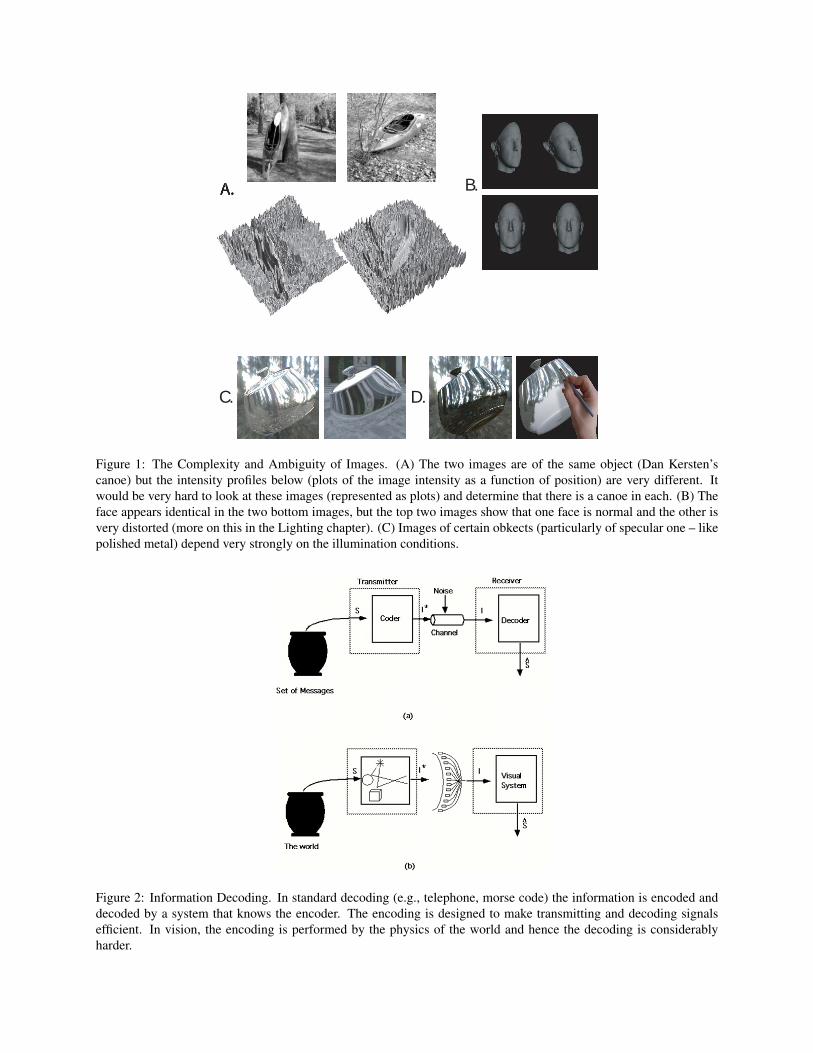
Why is vision difficult? The world W is complex and ambiguous, see figure (1) – the world consists of many objects(20,000 based on estimates made by counting the names of objects in dictionaries) and plenty of ”stuff” (texture,vegetation, etc.). The mapping from the world W to the image I is very complex – the image is generated by light raysbouncing off objects and reaching the eye/camera. Images are like an encoding of the world, but it is an encoding thatis not designed for communication (unlike speech, or morse code, or telephones), see figure (2). Decoding an imageI to determine the state of the world W that caused it is extremely difficult. The difficulty was first appreciated whenAI workers started trying to design computer vision systems (originally thinking it would only take a summer).

Another way to understand the complexity of images is by looking at how many images there can be. A typical imagesis 1, 024× 1, 024 pixels. Each pixel can take values 1− 255. This gives a number of images to be (1, 024× 1, 024)256

which is enormous (much much bigger than the number of atoms in the Universe). If you only consider 10 × 10images, you find there are more of them than can have been seen by all humans over evolutionary history (allowing 40year for life, 30 images a second, and other plausible assumptions). So the space of images is really enormous.

If vision is so hard then how is it possible to see? Several people (Gibson, Marr) have proposed ”ecological constraints”and ”natural constraints” which mean that the nature of the world provides constraints which reduce the ambiguities ofimages (e.g., most surfaces are smooth, most objects move rigidly). More recently, due to the growing availability ofdatasets (some with groundtruth) it has become possible to determine statistical regularities and statistical constraints(as will be described in this course). In short, there must be a lot of structure and regularity in images I , the world W ,and their relationship which can be exploited in order to make vision possible.

But how can we learn these structures/regularities? How can infants learn them and develop the sophisticated humanvisual system? How can researchers learn them and build working computer vision systems? It seems incrediblydifficult, if not impossible, to learn a full vision system in one go. Instead it seems that the only hope is proceed

A. B.

C. D.

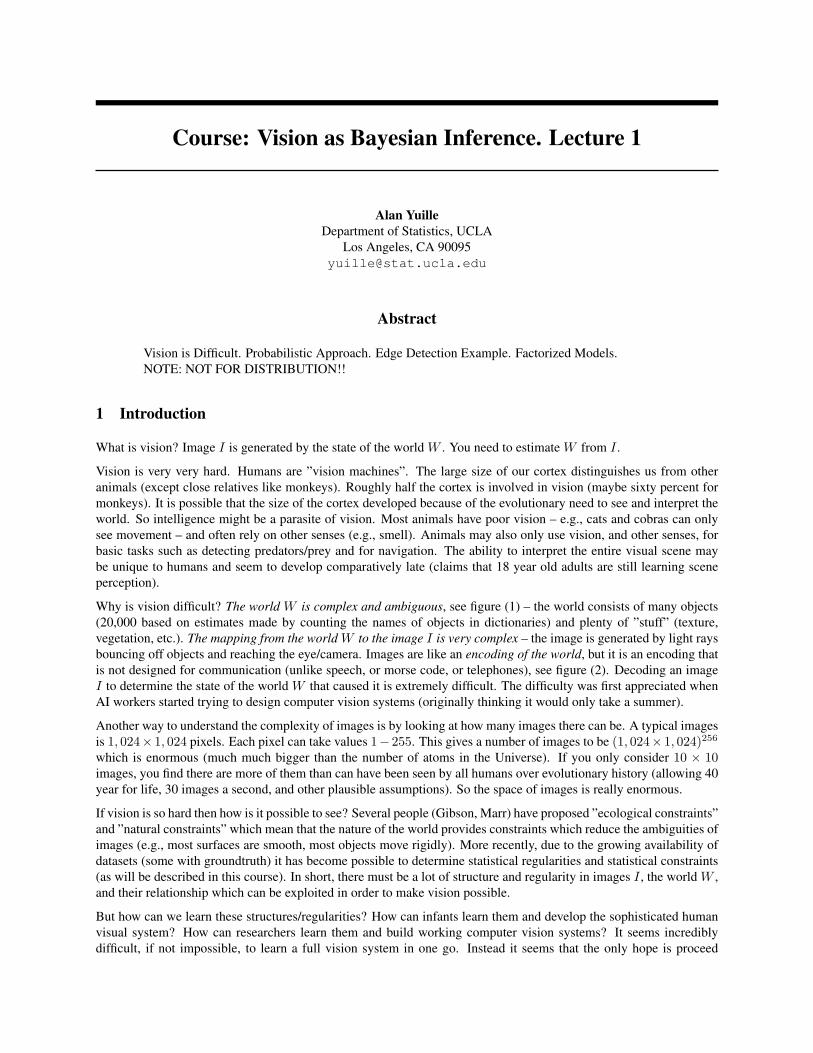
Figure 1: The Complexity and Ambiguity of Images. (A) The two images are of the same object (Dan Kersten’scanoe) but the intensity profiles below (plots of the image intensity as a function of position) are very different. Itwould be very hard to look at these images (represented as plots) and determine that there is a canoe in each. (B) Theface appears identical in the two bottom images, but the top two images show that one face is normal and the other isvery distorted (more on this in the Lighting chapter). (C) Images of certain obkects (particularly of specular one – likepolished metal) depend very strongly on the illumination conditions.

Figure 2: Information Decoding. In standard decoding (e.g., telephone, morse code) the information is encoded anddecoded by a system that knows the encoder. The encoding is designed to make transmitting and decoding signalsefficient. In vision, the encoding is performed by the physics of the world and hence the decoding is considerablyharder.

incrementally learning the simpler parts of vision first and then proceeding to the more complex parts. The study ofinfants (e.g., Kellman) suggests that visual abilities develop in an orchestrated manner with certain abilities developingwithin particular time periods – and, in particular, infants are able to perform motion tasks before they can deal withstatic images. Hence vision may be developed as a series of modules where easily learnable modules may be used asprequisites to train more complex modules.

But why is this incremental/modular strategy possible? Why is it possible to vision incrementally? (You cannot learnto ride a bicycle or parachuting incrementally). Stuart Geman suggests this is because the structure of the world,and of images, is compositional (i.e., is build out of elementary parts). He provocatively suggests that if the world isnot compositional then God exists! What he means that if the world/images are compositional (i.e. can be built upfrom elementary parts) then it is possible to imagine that an infant could learn these models. But if the world is non-compositional, then it seems impossible to understand how an infant could learnt at all (the idea of compositionalitywill be clarified as the course develops). Less religiously, Chomsky in the 1950’s proposed that language grammarswere innate (i.e., specified in the genes) because of the apparent difficulty of learning them (it is known that childrendevelop grammars even if they are not formally taught – e.g., children of slaves). But this raises the question ofhow genes could ”learn the grammars” in the first place. Others (e.g., Hinton) have questioned whether genes canconvey enough information to specify grammars (at least for vision). Recent computational work, however, (Kleinand Manning) has shown that grammars can, in fact, be learnt in an unsupervised manner (partially supervised – atleast, the system must know something about the form of the grammar if not the parameter values). It seem moreplausible that the brain has the ability to learn complex patterns (for vision, speech, language). But this only seemspossible if the world is compositional. These ideas of compositionality and modularity will be developed during thecourse.

2 How to formally approach vision?

How to formulate vision taking into account the (unknown) structures/regularities and compositionality/modularity?

This course argues that vision should be formulated in terms of probability distributions formulated on structured rep-resentations (e.g., graphs and grammars). In the last few years, there has been a revolution in the scope of probabilisticmodeling arising from combining ideas/concepts from Computer Science, Engineering, Mathematics, and Statistics.This revolution has been lead by the machine learning, neural networks, cognitive modeling, and artificial intelligencecommunities inspired by the need to design artificial systems capable of performing ”intelligent tasks” (and also beresearchers attempting to understand the complexities of human intelligence).

One main idea here is the formulation of vision as Bayesian inference. The idea is that we have probability distributionsP (I|W ) for the image generation process and P (W ) for the state of the world. Then vision reduces to interpretingW ∗ = arg maxP (W |I), where P (W |I) = P (I|W )P (W )/P (I). In vision, these ideas date back to Grenander’sconcept of Pattern Theory Grenander (1950’s-1990’s) was ahead of his time (slowness of computers, lack of effectiveinference algorithms, lack of knowledge about the complexities of vision).

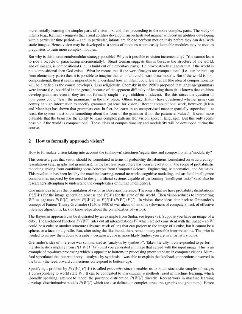
The Bayesian approach can be illustrated by an example from Sinha, see figure (3). Suppose you have an image of acube. The likelihood function P (I|W ) rules out all interpretations W which are not consistent with the image – so Wcould be a cube or another structure (abstract work of art) that can project to the image of a cube, but it cannot be asphere, or a face, or a giraffe. But, after using the likelihood, there remain many possible interpretations. The prior isneeded to narrow them down to a cube – because a cube is more likely (unless you are in an artist’s studio).

Grenander’s idea of inference was summarized as ”analysis by synthesis”. Taken literally, it corresponded to perform-ing stochastic sampling from P (I|W )P (W ) until you generated an image that agreed with the input image. This is anexample of top-down processing which is opposite to bottom-up processing (more standard in computer vision). Mum-ford speculated that pattern theory – analysis by synthesis – was able to explain the feedback connections observed inthe brain (the feedforward connections correspond to bottom-up).

Specifying a problem by P (I|W )P (W ) is called generative since it enables us to obtain stochastic samples of imagesI corresponding to world state W . It can be contrasted to discriminative methods, used in machine learning, which(broadly speaking) attempt to model the posterior distribution P (W |I) directly. Recent work in machine learningdevelops discriminative models P (W |I) which are also defined on complex structures (graphs and grammars). Hence

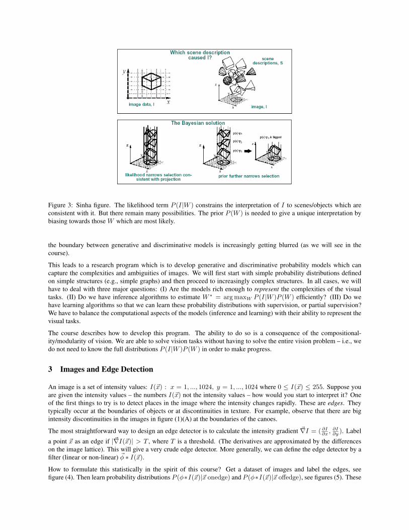
Figure 3: Sinha figure. The likelihood term P (I|W ) constrains the interpretation of I to scenes/objects which areconsistent with it. But there remain many possibilities. The prior P (W ) is needed to give a unique interpretation bybiasing towards those W which are most likely.

the boundary between generative and discriminative models is increasingly getting blurred (as we will see in thecourse).

This leads to a research program which is to develop generative and discriminative probability models which cancapture the complexities and ambiguities of images. We will first start with simple probability distributions definedon simple structures (e.g., simple graphs) and then proceed to increasingly complex structures. In all cases, we willhave to deal with three major questions: (I) Are the models rich enough to represent the complexities of the visualtasks. (II) Do we have inference algorithms to estimate W ∗ = arg maxW P (I|W )P (W ) efficiently? (III) Do wehave learning algorithms so that we can learn these probability distributions with supervision, or partial supervision?We have to balance the computational aspects of the models (inference and learning) with their ability to represent thevisual tasks.

The course describes how to develop this program. The ability to do so is a consequence of the compositional-ity/modularity of vision. We are able to solve vision tasks without having to solve the entire vision problem – i.e., wedo not need to know the full distributions P (I|W )P (W ) in order to make progress.

3 Images and Edge Detection

An image is a set of intensity values: I(~x) : x = 1, ..., 1024, y = 1, ..., 1024 where 0 ≤ I(~x) ≤ 255. Suppose youare given the intensity values – the numbers I(~x) not the intensity values – how would you start to interpret it? Oneof the first things to try is to detect places in the image where the intensity changes rapidly. These are edges. Theytypically occur at the boundaries of objects or at discontinuities in texture. For example, observe that there are bigintensity discontinuities in the images in figure (1)(A) at the boundaries of the canoes.

The most straightforward way to design an edge detector is to calculate the intensity gradient ~∇I = ( ∂I∂x ,∂I∂y ). Label

a point ~x as an edge if |~∇I(~x)| > T , where T is a threshold. (The derivatives are approximated by the differenceson the image lattice). This will give a very crude edge detector. More generally, we can define the edge detector by afilter (linear or non-linear) ~φ ∗ I(~x).

How to formulate this statistically in the spirit of this course? Get a dataset of images and label the edges, seefigure (4). Then learn probability distributions P (φ∗I(~x)|~x onedge) and P (φ∗I(~x)|~x offedge), see figures (5). These

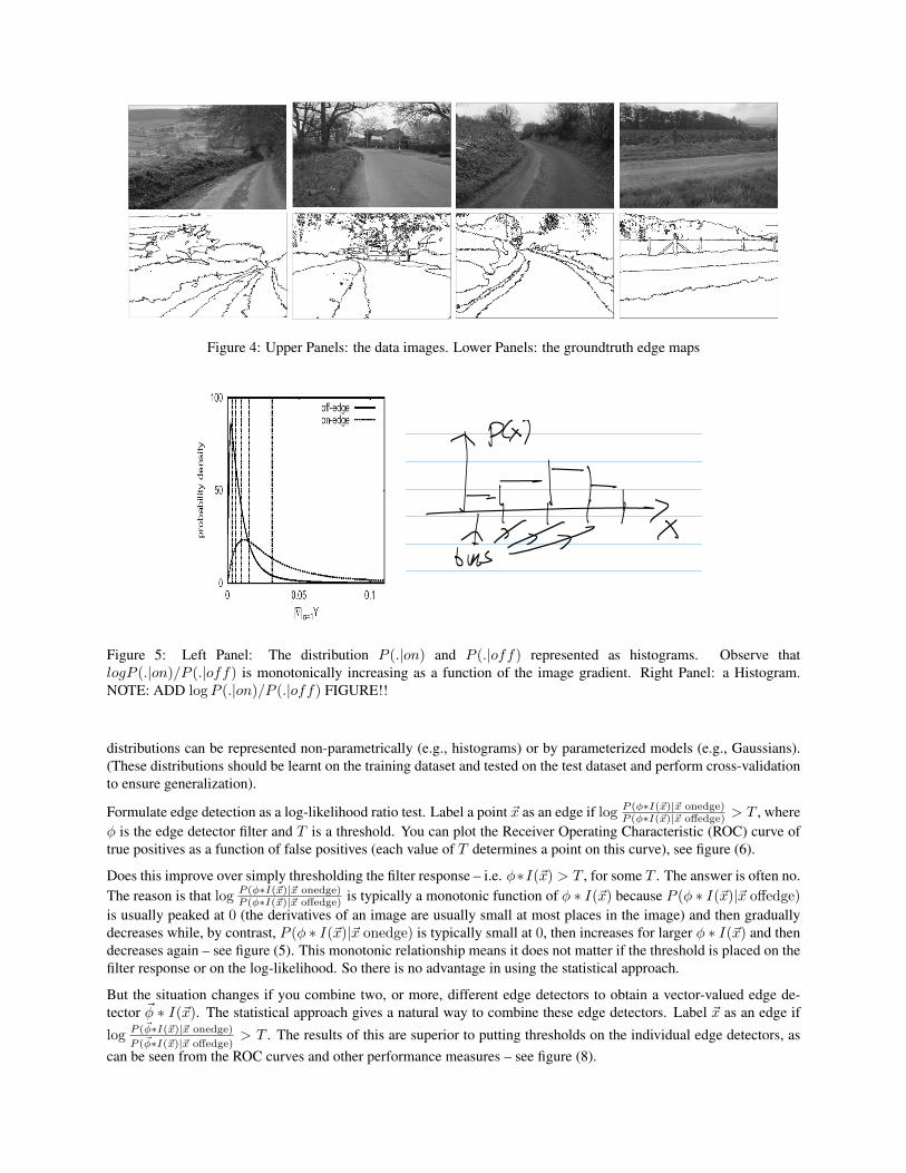
Figure 4: Upper Panels: the data images. Lower Panels: the groundtruth edge maps

Figure 5: Left Panel: The distribution P (.|on) and P (.|off) represented as histograms. Observe thatlogP (.|on)/P (.|off) is monotonically increasing as a function of the image gradient. Right Panel: a Histogram.NOTE: ADD logP (.|on)/P (.|off) FIGURE!!

distributions can be represented non-parametrically (e.g., histograms) or by parameterized models (e.g., Gaussians).(These distributions should be learnt on the training dataset and tested on the test dataset and perform cross-validationto ensure generalization).

Formulate edge detection as a log-likelihood ratio test. Label a point ~x as an edge if log P (φ∗I(~x)|~x onedge)P (φ∗I(~x)|~x offedge) > T , where

φ is the edge detector filter and T is a threshold. You can plot the Receiver Operating Characteristic (ROC) curve oftrue positives as a function of false positives (each value of T determines a point on this curve), see figure (6).

Does this improve over simply thresholding the filter response – i.e. φ∗I(~x) > T , for some T . The answer is often no.The reason is that log P (φ∗I(~x)|~x onedge)

P (φ∗I(~x)|~x offedge) is typically a monotonic function of φ ∗ I(~x) because P (φ ∗ I(~x)|~x offedge)is usually peaked at 0 (the derivatives of an image are usually small at most places in the image) and then graduallydecreases while, by contrast, P (φ ∗ I(~x)|~x onedge) is typically small at 0, then increases for larger φ ∗ I(~x) and thendecreases again – see figure (5). This monotonic relationship means it does not matter if the threshold is placed on thefilter response or on the log-likelihood. So there is no advantage in using the statistical approach.

But the situation changes if you combine two, or more, different edge detectors to obtain a vector-valued edge de-tector ~φ ∗ I(~x). The statistical approach gives a natural way to combine these edge detectors. Label ~x as an edge if

log P (~φ∗I(~x)|~x onedge)

P (~φ∗I(~x)|~x offedge)> T . The results of this are superior to putting thresholds on the individual edge detectors, as

can be seen from the ROC curves and other performance measures – see figure (8).

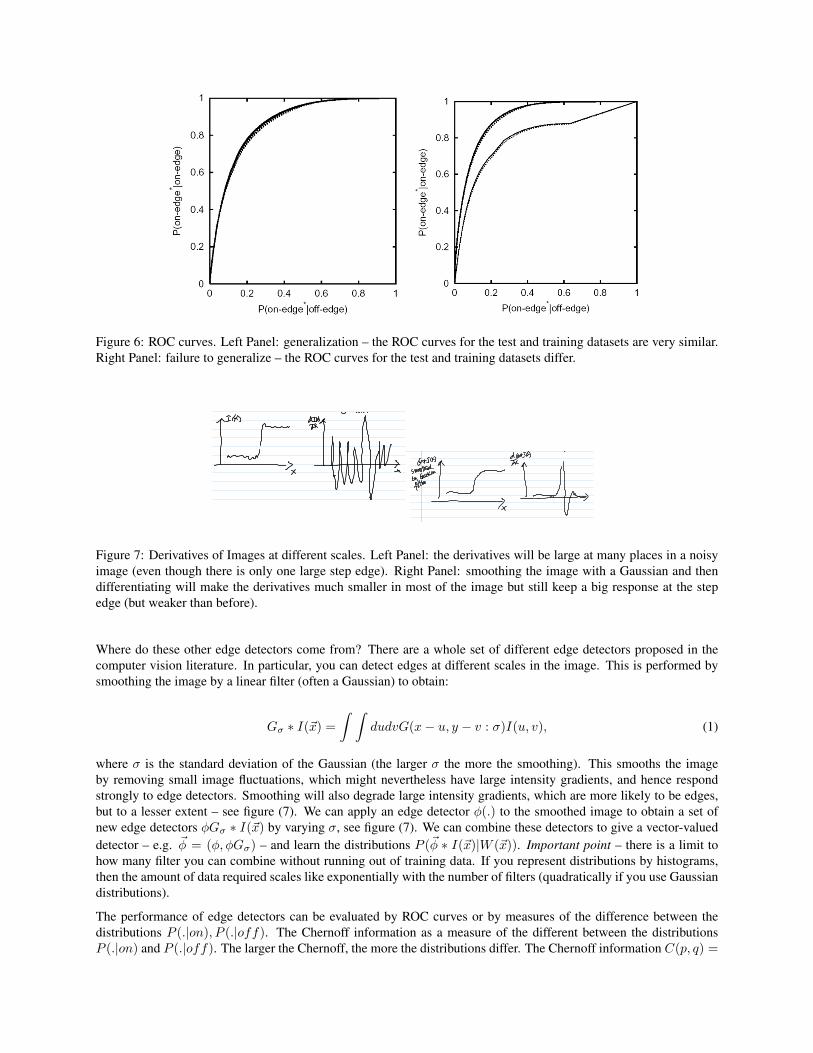
Figure 6: ROC curves. Left Panel: generalization – the ROC curves for the test and training datasets are very similar.Right Panel: failure to generalize – the ROC curves for the test and training datasets differ.

Figure 7: Derivatives of Images at different scales. Left Panel: the derivatives will be large at many places in a noisyimage (even though there is only one large step edge). Right Panel: smoothing the image with a Gaussian and thendifferentiating will make the derivatives much smaller in most of the image but still keep a big response at the stepedge (but weaker than before).

Where do these other edge detectors come from? There are a whole set of different edge detectors proposed in thecomputer vision literature. In particular, you can detect edges at different scales in the image. This is performed bysmoothing the image by a linear filter (often a Gaussian) to obtain:

Gσ ∗ I(~x) =∫ ∫

dudvG(x− u, y − v : σ)I(u, v), (1)

where σ is the standard deviation of the Gaussian (the larger σ the more the smoothing). This smooths the imageby removing small image fluctuations, which might nevertheless have large intensity gradients, and hence respondstrongly to edge detectors. Smoothing will also degrade large intensity gradients, which are more likely to be edges,but to a lesser extent – see figure (7). We can apply an edge detector φ(.) to the smoothed image to obtain a set ofnew edge detectors φGσ ∗ I(~x) by varying σ, see figure (7). We can combine these detectors to give a vector-valueddetector – e.g. ~φ = (φ, φGσ) – and learn the distributions P (~φ ∗ I(~x)|W (~x)). Important point – there is a limit tohow many filter you can combine without running out of training data. If you represent distributions by histograms,then the amount of data required scales like exponentially with the number of filters (quadratically if you use Gaussiandistributions).

The performance of edge detectors can be evaluated by ROC curves or by measures of the difference between thedistributions P (.|on), P (.|off). The Chernoff information as a measure of the different between the distributionsP (.|on) and P (.|off). The larger the Chernoff, the more the distributions differ. The Chernoff information C(p, q) =

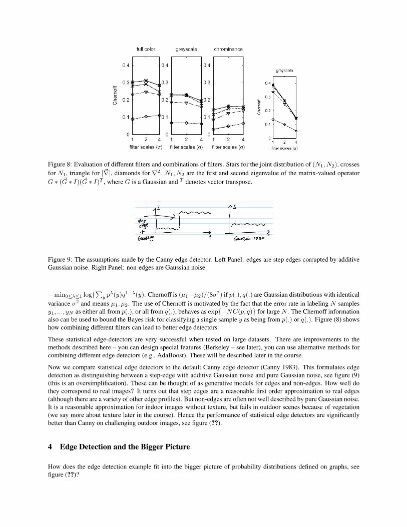
Figure 8: Evaluation of different filters and combinations of filters. Stars for the joint distribution of (N1, N2), crossesfor N1, triangle for |~∇|, diamonds for ∇2. N1, N2 are the first and second eigenvalue of the matrix-valued operatorG ∗ (~G ∗ I)(~G ∗ I)T , where G is a Gaussian and T denotes vector transpose.

Figure 9: The assumptions made by the Canny edge detector. Left Panel: edges are step edges corrupted by additiveGaussian noise. Right Panel: non-edges are Gaussian noise.

−min0≤λ≤1 log{∑y p

λ(y)q1−λ(y). Chernoff is (µ1−µ2)/(8σ2) if p(.), q(.) are Gaussian distributions with identicalvariance σ2 and means µ1, µ2. The use of Chernoff is motivated by the fact that the error rate in labeling N samplesy1, ..., yN as either all from p(.), or all from q(.), behaves as exp{−NC(p, q)} for large N . The Chernoff informationalso can be used to bound the Bayes risk for classifying a single sample y as being from p(.) or q(.). Figure (8) showshow combining different filters can lead to better edge detectors.

These statistical edge-detectors are very successful when tested on large datasets. There are improvements to themethods described here – you can design special features (Berkeley – see later), you can use alternative methods forcombining different edge detectors (e.g., AdaBoost). These will be described later in the course.

Now we compare statistical edge detectors to the default Canny edge detector (Canny 1983). This formulates edgedetection as distinguishing between a step-edge with additive Gaussian noise and pure Gaussian noise, see figure (9)(this is an oversimplification). These can be thought of as generative models for edges and non-edges. How well dothey correspond to real images? It turns out that step edges are a reasonable first order approximation to real edges(although there are a variety of other edge profiles). But non-edges are often not well described by pure Gaussian noise.It is a reasonable approximation for indoor images without texture, but fails in outdoor scenes because of vegetation(we say more about texture later in the course). Hence the performance of statistical edge detectors are significantlybetter than Canny on challenging outdoor images, see figure (??).

4 Edge Detection and the Bigger Picture

How does the edge detection example fit into the bigger picture of probability distributions defined on graphs, seefigure (??)?

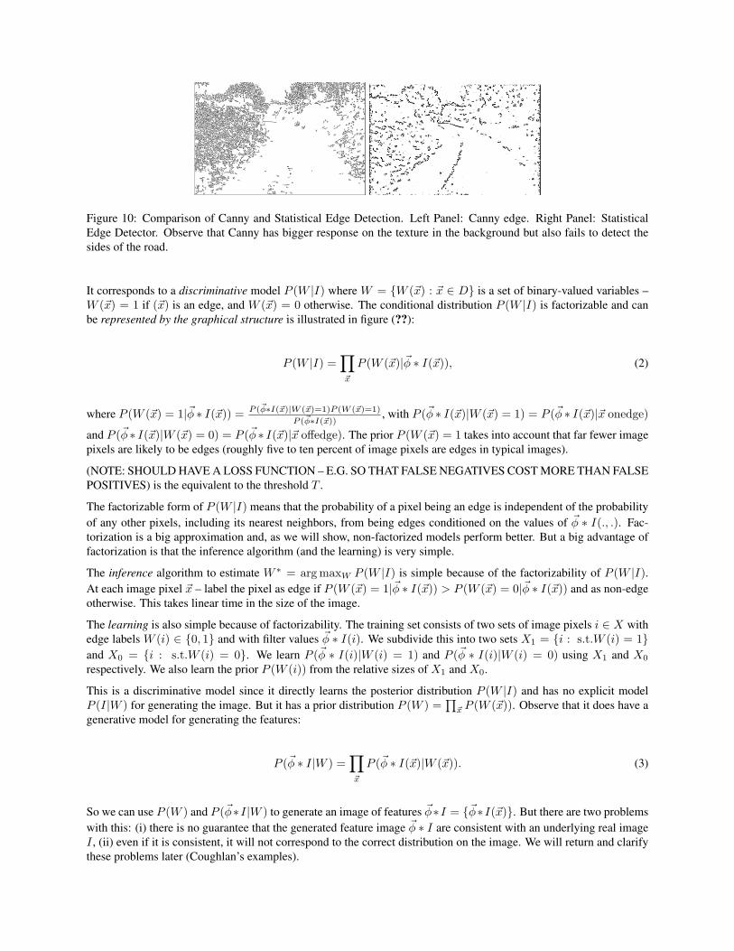
Figure 10: Comparison of Canny and Statistical Edge Detection. Left Panel: Canny edge. Right Panel: StatisticalEdge Detector. Observe that Canny has bigger response on the texture in the background but also fails to detect thesides of the road.

It corresponds to a discriminative model P (W |I) where W = {W (~x) : ~x ∈ D} is a set of binary-valued variables –W (~x) = 1 if (~x) is an edge, and W (~x) = 0 otherwise. The conditional distribution P (W |I) is factorizable and canbe represented by the graphical structure is illustrated in figure (??):

P (W |I) =∏~x

P (W (~x)|~φ ∗ I(~x)), (2)

where P (W (~x) = 1|~φ ∗ I(~x)) = P (~φ∗I(~x)|W (~x)=1)P (W (~x)=1)

P (~φ∗I(~x)), with P (~φ ∗ I(~x)|W (~x) = 1) = P (~φ ∗ I(~x)|~x onedge)

and P (~φ ∗ I(~x)|W (~x) = 0) = P (~φ ∗ I(~x)|~x offedge). The prior P (W (~x) = 1 takes into account that far fewer imagepixels are likely to be edges (roughly five to ten percent of image pixels are edges in typical images).

(NOTE: SHOULD HAVE A LOSS FUNCTION – E.G. SO THAT FALSE NEGATIVES COST MORE THAN FALSEPOSITIVES) is the equivalent to the threshold T .

The factorizable form of P (W |I) means that the probability of a pixel being an edge is independent of the probabilityof any other pixels, including its nearest neighbors, from being edges conditioned on the values of ~φ ∗ I(., .). Fac-torization is a big approximation and, as we will show, non-factorized models perform better. But a big advantage offactorization is that the inference algorithm (and the learning) is very simple.

The inference algorithm to estimate W ∗ = arg maxW P (W |I) is simple because of the factorizability of P (W |I).At each image pixel ~x – label the pixel as edge if P (W (~x) = 1|~φ ∗ I(~x)) > P (W (~x) = 0|~φ ∗ I(~x)) and as non-edgeotherwise. This takes linear time in the size of the image.

The learning is also simple because of factorizability. The training set consists of two sets of image pixels i ∈ X withedge labels W (i) ∈ {0, 1} and with filter values ~φ ∗ I(i). We subdivide this into two sets X1 = {i : s.t.W (i) = 1}and X0 = {i : s.t.W (i) = 0}. We learn P (~φ ∗ I(i)|W (i) = 1) and P (~φ ∗ I(i)|W (i) = 0) using X1 and X0

respectively. We also learn the prior P (W (i)) from the relative sizes of X1 and X0.

This is a discriminative model since it directly learns the posterior distribution P (W |I) and has no explicit modelP (I|W ) for generating the image. But it has a prior distribution P (W ) =

∏~x P (W (~x)). Observe that it does have a

generative model for generating the features:

P (~φ ∗ I|W ) =∏~x

P (~φ ∗ I(~x)|W (~x)). (3)

So we can use P (W ) and P (~φ∗I|W ) to generate an image of features ~φ∗I = {~φ∗I(~x)}. But there are two problemswith this: (i) there is no guarantee that the generated feature image ~φ ∗ I are consistent with an underlying real imageI , (ii) even if it is consistent, it will not correspond to the correct distribution on the image. We will return and clarifythese problems later (Coughlan’s examples).

5 Labelling Image Regions

We can apply the same approach to the task of labeling image pixels as a number of discrete regions – e.g., sky, road,vegetation, other. To do this we define W = {W (~x)} so that W (~x) ∈ L, where L = {sky, road, vegetation, other}is a set of labels. We use similar filters ~φ(.) as before to learn distributions P (~φ ∗ I(~x)|W (~x)) for W (~x) ∈ L.

This results in a factorized model of similar form to equation (2) and with similar graph structure:

P (W |I) =∏~x

P (W (~x)|~φ ∗ I(~x)), (4)

The learning and inference are simple generalizations of those for the binary task of edge detection. The only differenceis the large number of labels.

This simple model does surprisingly well. If the filters use color or texture or a combination – then they can achievevery high accuracy on labeling regions such as sky, road and vegetation. This success happens because these regionsare comparatively homogeneous (i.e. all parts of the sky as similar to each other – FULL DEFINITION OF HO-MOGENEITY SOMEWHERE??). But it is less successful for detecting non-homogeneous objects like houses. Thismotivates more advanced non-factorizable models which will be described later in the course.

PUT A FIGURE TO ILLUSTRATE KONISHI’S RESULTS ON REGIONS!!

6 Bayes Decision Theory and Loss Functions

So far, we have assumed that the goal of inference is to obtain the Maximum a Posteriori (MAP) estimate W ∗ =arg maxW P (W |I). But why? Where does this come from? What are the alternatives?

The basis is Bayes Decision Theory which formulates problems as minimizing the expected loss. To make this precise,assume we have a joint distribution P (W, I), a set Λ of decision rules α(.), and a loss function L(α(I),W ) for makingdecision α(I) for input I when the true state is W .

Bayes Decision Theory states that you should pick the decision rule that minimize the risk which is defined to be theexpected loss:

R(α) =∑I,W

L(α(I),W )P (I,W ), (5)

where we replace the summations by integrals if I , W , or both are continuous valued.

Bayes Rule α∗ = arg minα∈Λ

R(α), Bayes Risk R(α∗) = minα∈Λ

R(α). (6)

NOTE: there are a few mathematical special cases where R(α∗) 6= arg minα∈ΛR(α) but they very rarely occuroutside mathematics books.

We can re-express the risk as:

R(α) =∑I

P (I)R(α|I), whereR(α|I) =∑W

L(α(I),W )P (W |I). (7)

Hence minimizing the Bayes risk is equivalent to minimizing the conditional risk R(α|I) for each I (i.e., the Bayesdecision rule for input I is independent of its decision for other inputs – alternatively, the distribution P (I) has noeffect on determining the Bayes rule). This gives:

α∗(I) = arg minα(I)

∑W

L(α(I),W )P (W |I), discrete W

α∗(I) = arg minα(I)

∫dWL(α(I),W )P (W |I), continuous W. (8)

The MAP estimate arises as a special case for a particular choice of loss function.

In the discrete case, set L(α(I),W ) = 1− δ(α(I),W ), where the delta function δ(α(I),W ) takes value 1 if α(I) =W and value 0 otherwise (i.e., correct responses pay no penalty but incorrect responses are weighted the same). TheBayes rule reduces to maximizing

∑W δ(α(I),W )P (W |I) = P (W = α(I)|I), which is the MAP estimate.

For certain applications – e.g., edge detection, face detection – it may be better to use a different loss function whichpenalizes false negatives (failure to find edges/faces) more than false positive (finding edges/faces where they do notexist). The reason is that we can use later processing (i.e., other models) to eliminate the false positives. But it isharder to resurrect the false negatives.

In the continuous case, set L(α(I),W ) = −δ(α(I)−W ), where δ(.) is the Dirac delta function (i.e., δ(x) = 0, x 6= 0and

∫dxδ(x) = 1, provided the range of integration contains the point x = 0. The Bayes rule reduces to maximizing∫

dWδ(α(I),W )P (W |I) = P (W = α(I)|I) which is the MAP estimator.

Observe that the Dirac delta function is a strange choice of loss function because it pays an (infinite) penalty unlessthe decision is perfectly correct. There is no partial credit for making a decision α(I) that differs from the correctdecision W by an infinitesimal amount. This is highly unrealistic. More reasonable choices of loss function are to setL(α(I),W ) = −G(α(I) −W : σ), where G is a Gaussian whose variance/covariance determines how much partialcredit to give. In practice, the simplicity of MAP estimation – and the difficulty of determining how to assign partialcredit – means that MAP estimation is often used in practice. Alternatives will be described later in the course. Theyinclude the mean estimate

∫P (W |I)WdW which occurs for quadratic loss function L(α(I),W ) = (α(I)−W )2. In

summary, MAP estimation for continuous variables should be used with caution.

Bayes decision theory and approximate models. There is a simple but important conceptual point to be made from theBayes Risk (which several well-known vision researchers have got wrong!). The Bayes risk is obtained by minimizingwith respect to all decision rules. If we reduce the set of allowable decision rules, for example if we do edge detectionwith a restricted class of filters, then we have to do worse.

Bayes decision theory has some implications which may be counter-intuitive. Suppose the likelihood term P (I|W )is sufficient to determine the correct W . Then the prior P (W ) may bias the result. The reason is that Bayes decisiontheory assumes that you should make the best decision on average, which does not correspond to making the bestdecision on a specific example. Bayes decision theory can be a bad guide for how to make one-time only decisions– such as buying a house, or gambling on the stock market. In such case, it may be wiser to take into account theworst-case loss rather than the average case (i.e., how much money can you afford to loss in the stock market). Butthe mathematics for this is much more complicated and worrying about the worst case is often paranoid.

Appendices

A1: Filters: Discrete and Continuous

Although images are defined on a discrete image lattice it is often convenient to formulate theories on continuousimage domain and then discretize them.

For continuous images I(~x) : ~x ∈ D, we define (spatial invariant) linear filtering by a filter φ(u, v) to be:

φ ∗ I(~x) =∫ ∫

dudvφ(x− u, y − v)I(u, v). (9)

This is convolution. We can apply Fourier transforms to obtain φ(ωx, ωy) = φ(ωx, ωy)I(ωx, ωy), where (ωx, ωy) isfrequency. HOW MUCH TO SAY ABOUT FOURIER THEORY??

For discrete images I(~x) : x = 1, ..., 1024 y = 1, ..., 1024 and a discrete filter φ(u, v), we define a linear filter to be:

φ ∗ I(~x) =∑u

∑v

φ(x− u, y − v)I(u, v). (10)

The simplest filters are derivatives –e.g. d/dx and d/dy. These can be converted into discrete filters such as 1,−1 (inone dimension). Better derivative approximations can be performed (see standard textbooks).

Standard classes of filters. Derivatives of Gaussians. The idea is that the Gaussians smooth the image.

Other filters are Gabors: G(~x) = 12π|Σ exp{−(1/2)~xTΣ−1~x} exp i(ωxx+ ωyy), where (ωx, ωy) is in the direction

of the second eigenvector of Σ. The Gabor filter is complex and can be decomposed into a cosine Gabor (the real part)and a sine Gabor (the imaginary part) (exp{iθ} = cos θ + i sin θ). Energy filters are defined by summing the cosineand sine parts.

Discuss wavelets.

A2: Image Formation

How are images formed?

Light rays hit objects and get reflected. This will be described in later chapters. There is Computer Graphics where thegoal is to generate realistic images. This involves studies of models for how objects reflect light (radiosity models).Computer vision can be formulated as inverting this process. But unfortunately this is much harder. For certain typesof illumination models this is relatively easy (e.g. Lambertian models) but for others it is very difficult. Learning maybe more useful than Physics based models.

Cameras, focal points, blurring, and so on. We need to say something about this. People should be aware of the factorsinvolved.

NEED SOME BACKGROUND MATERIAL HERE!! BUT NOT CRITICAL FOR THE COURSE!!

A3: Learning – Memorizing and Generalizing

The study of Machine Learning has taught us a lot about the differences of generalizing and memorizing.

All learning is done from a finite training set of data {(xi, yi) : i = 1, ..., N} but we want decision rules to be valid fordata that we have not seen yet. Most studies of this problem assume that the data samples are independent identicallydistributed (i.i.d.) from some unknown distribution P (~x). We design a decision rule α(.) ∈ Λ which maps x to y. Wechoose a loss function L(α(x), y) which is the penalty for making decision α(x) for data x when the true decision isy (i.e., usually L(α(x), y) = 0 if α(x) = y).

From the training dataset, we can learn a decision rule α to make the empirical risk small, where the empirical risk(average loss over the training dataset) is defined by:

Remp(α) =1N

M∑i=1

L(α(xi), yi). (11)

But this is only memorization (i.e., applies only to the training data) unless α also minimizes the risk (expected loss)of all the samples from the distribution:

R(α) =∑x

∑y

P (~x)L(α(x), y). (12)

Memorization typically occurs when the amount N of training data is small and the set Λ of possible α(.) is large(technically the capacity). In this situation, it is too easy to find a decision rule that gives a good fit to the training databy chance (this is how conspiracy theories get started).

To obtain generalization, we require that R(α) ≈ Remp(α) (over-simplified?). How can we be sure that this is thecase?

For certain classes of problem (making decisions) there is a beautiful theory due to Vapnik (see also Valiant) whichshows that with probability greater than 1− δ that

R(α) ≤ Remp(α) + φ(N,h, δ). (13)

where h is the VC dimension which is a measure of the capacity of the set of classifiers α ∈ Λ. Provided N ismuch large than h and than | log δ| then we can be sure that minimizing Remp will make R small. But this theory isunfortunately mostly of conceptual use because the bounds are often not tight enough. The theory is slightly paranoidbecause it has to rule out the probability that a rule might classify the training data correctly because of a chancestructure in the dataset (e.g. in high-dimension space d and only N datapoints it is always possible to get a rule tomake any dichotomy).

Instead, in practice, we use the idea of cross-validation (of which there are many variants). This involves a trainingdataset and a test dataset. The decision rule is learnt on the training dataset and evaluated on the test dataset (this canbe thought of as using the test dataset to estimate the Bayes risk). This is not rigorously guaranteeing that R(α) ≈Remp(α) (because there is always the chance that both training and test datasets are atypical of the distribution P (~x)).But how paranoid do you want to be?

A4: Adaption, Transfer Learning

Are all datasets the same? Suppose you learn an edge detector on one dataset – will it also work on another dataset?The answer is clearly not if the datasets come from different sources. E.g. suppose one dataset the images values havebeen thresholded to lie in the range 128− 136 (stranger things have happened in medical image datasets).

For example, the Soweby dataset and the South Florida dataset differ because Sowerby is taken outdoors in the Englishcountryside while South Florida is taken mainly indoors and with textured regions suppressed. Looking at the imagesmakes it easy to see that edges in the South Florida images are sharper.

Can you transfer learning from one domain to another? Or in biological terminology adapt (when one animal movesfrom the water to the land). For edges, this is not that hard by exploiting structure. I.e. you can estimates the filterstatistics in the background by simply computing the statistics over the entire image (and the edges are few enough toonly partially contaminate the data).

A5: Relations to Neuroscience

Computational neuroscientists model receptive field properties of neurons in the retina, LGN, and V1 (part of cortex)as linear and non-linear filters.

The receptive fields in the retina and LGN are often modeled as linear receptive fields. These models are believed to befairly reliable – in the sense that neuroscientists can predict the response of these neurons to novel stimuli, or determinethe image from the activity of the retina or LGN cells (Dan – check this!!). There has been some success (e.g, Atick) atderiving the linear receptive field properties of neurons in the retina and the LGN from information theoretic principles(i.e., the filters are designed to encode images so that they can be transmitted reliably and efficiently from the retinato the LGN and then from the LGN to the cortex (V1). The receptive field properties depend on the statistics on theinput images and so will change (adaption) as the statistics vary.

Receptive field properties in the early visual cortex are more complicated. It is sometimes stated that the receptivefields can be modeled by Gabor functions (simple cells) and squares of Gabor functions (complex cells), but this seemsonly approximate (Ringach). In particular, these models do not successfully predict the responses of the neurons to realimages (the experiments for measuring the receptive fields are performed on synthetic stimuli). There has been somesuccess in predicting receptive field properties by sparse coding ideas and independent component analysis (these willbe described later in the course).

A6: Relations to Machine Learning and Neural Networks

The ideas of memorization/generation were developed in the 1980’s. Valiant’ theory of the learning (two very shortpapers) inspired the development of PAC learning theory (Rivest). Vapnik’s work was highly respected by a smallgroup but only became seriously influential when Vapnik emigrated to the USA (from the Soviet Union) and his worklead to Support Vector Machines.

MOVE THIS TO SOMEWHERE WHERE WE DESCRIBE MORE SERIOUS LEARNING!!