Embed Size (px)
DESCRIPTION
Bayesian inference. calculate the model parameters that produce a distribution that gives the observed data the greatest probability. Thomas Bayes. Bayesian methods were invented in the 18 th century , but their application in phylogenetics dates from 1996. Thomas Bayes ? (1701?-1761?). - PowerPoint PPT Presentation
Citation preview
Bayesian inferencecalculate the model parameters that produce a distribution that gives the observed data the greatest probability
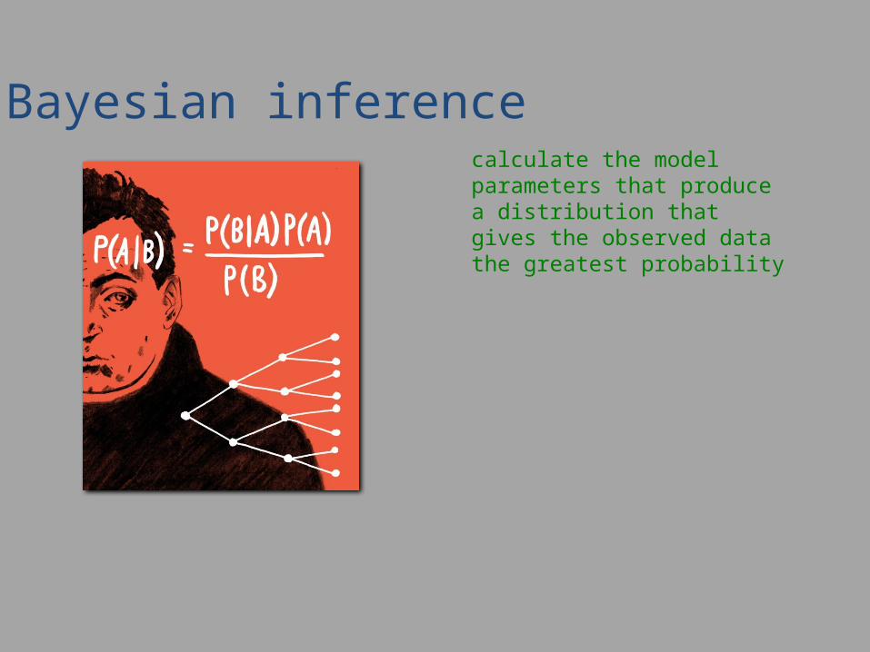
Thomas Bayes Bayesian methods were invented in the 18th century, but their application in phylogenetics dates from 1996.
Thomas Bayes? (1701?-1761?)
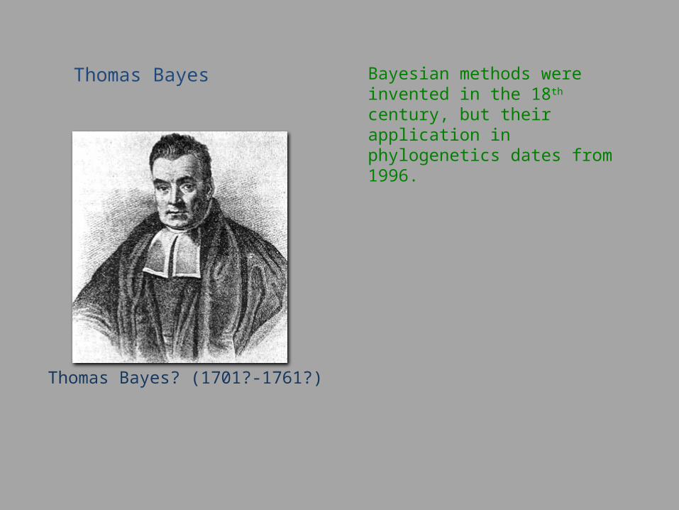
Bayes’ theorem Bayes’ theorema links a conditional probability to its inverse
Prob(H|D) = Prob(H) Prob(D|H)
∑H Prob(H) Prob(D|H)
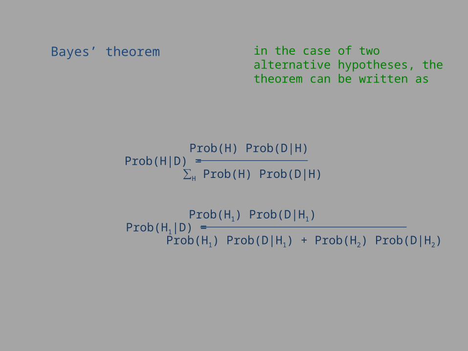
Bayes’ theorem in the case of two alternative hypotheses, the theorem can be written as
Prob(H|D) = Prob(H) Prob(D|H)
∑H Prob(H) Prob(D|H)
Prob(H1|D) = Prob(H1) Prob(D|H1)
Prob(H1) Prob(D|H1) + Prob(H2) Prob(D|H2)
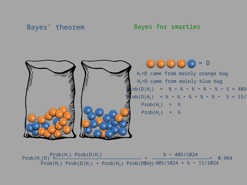
Bayes’ theorem Bayes for smarties
m
m
= D
H1=D came from mainly orange bag
H2=D came from mainly blue bag
Prob(D|H1) = ¾ • ¾ • ¾ • ¾ • ¼ • 5 = 405/1024
Prob(D|H2) = ¼ • ¼ • ¼ • ¼ • ¾ • 5 = 15/1024
Prob(H1) = ½
Prob(H2) = ½
Prob(H1|D) = Prob(H1) Prob(D|H1)
Prob(H1) Prob(D|H1) + Prob(H2) Prob(D|H2) = = 0.964
½ • 405/1024
½ • 405/1024 + ½ • 15/1024
m
m
mmm
mm
m
m
mm
mm
mm mmm m
mm
m
mmm m
m
m
m
m m
mm
mm
mm
m
m m m m
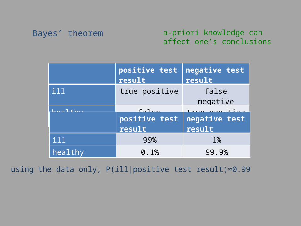
Bayes’ theorem a-priori knowledge can affect one’s conclusions
positive test result negative test result
ill true positive false negative
healthy false positive true negative
positive test result negative test result
ill 99% 1%
healthy 0.1% 99.9%
using the data only, P(ill|positive test result)≈0.99
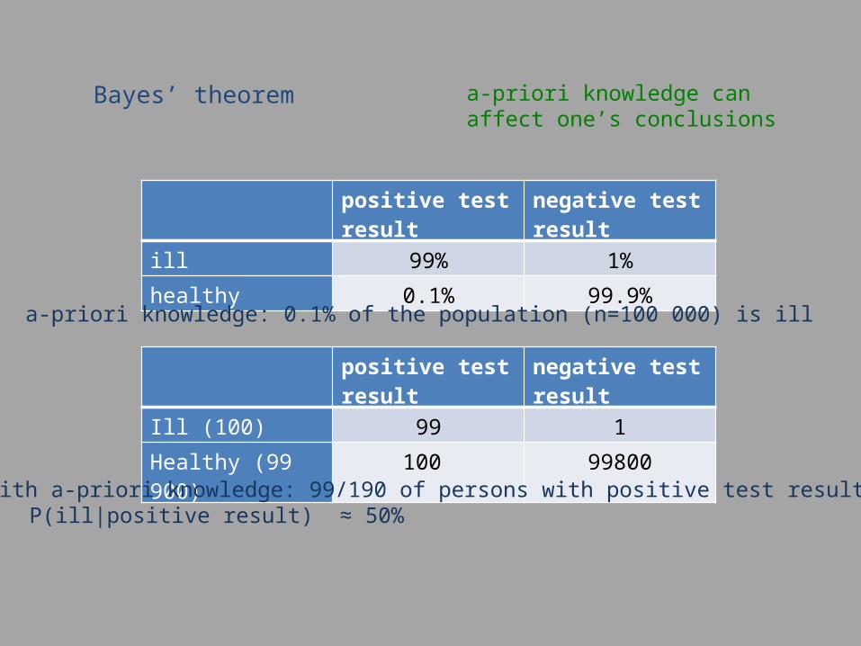
Bayes’ theorem a-priori knowledge can affect one’s conclusions
positive test result negative test result
ill 99% 1%
healthy 0.1% 99.9%
a-priori knowledge: 0.1% of the population (n=100 000) is ill
positive test result negative test result
Ill (100) 99 1
Healthy (99 900) 100 99800
with a-priori knowledge: 99/190 of persons with positive test results is ill P(ill|positive result) ≈ 50%
Bayes’ theorem a-priori knowledge can affect one’s conclusions
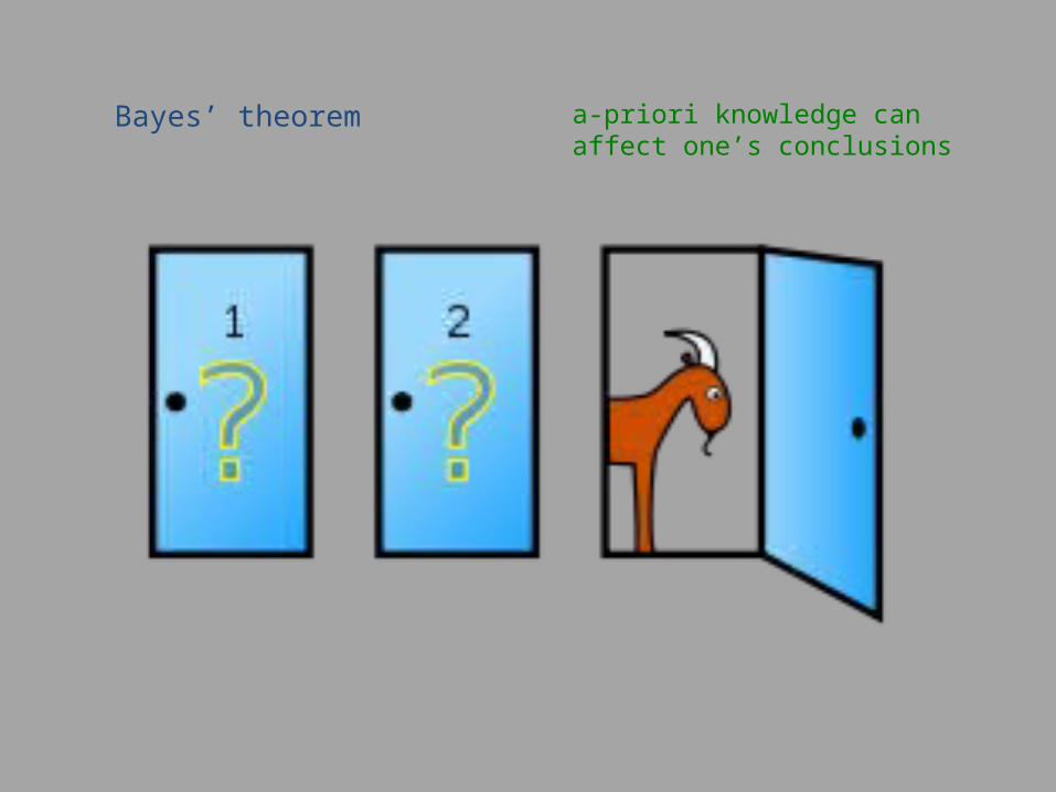
Bayes’ theorem a-priori knowledge can affect one’s conclusions
Bayes’ theorem a-priori knowledge can affect one’s conclusions
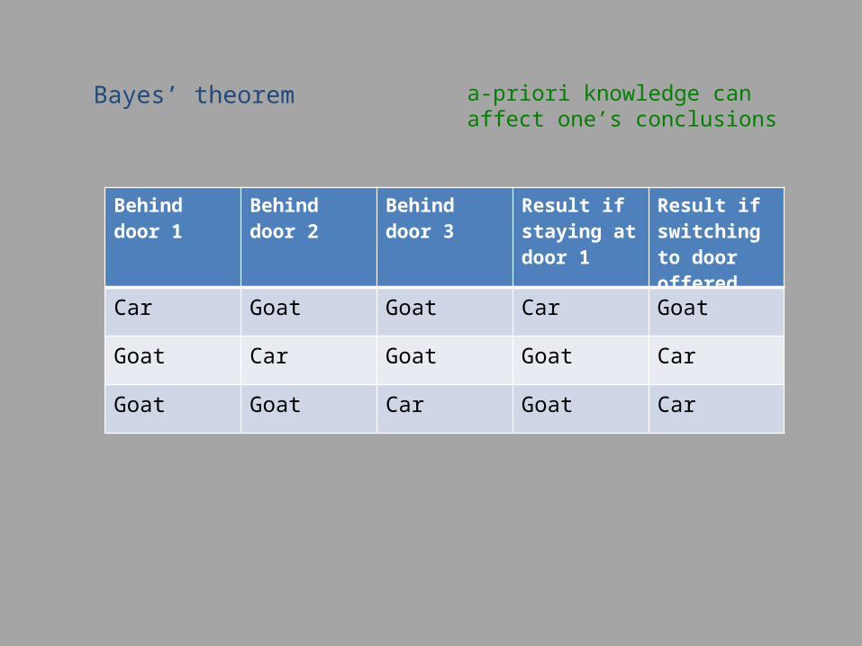
Behind door 1 Behind door 2 Behind door 3 Result if staying at door 1
Result if switching to door offered
Car Goat Goat Car Goat
Goat Car Goat Goat Car
Goat Goat Car Goat Car
Bayes’ theorem a-priori knowledge can affect one’s conclusions
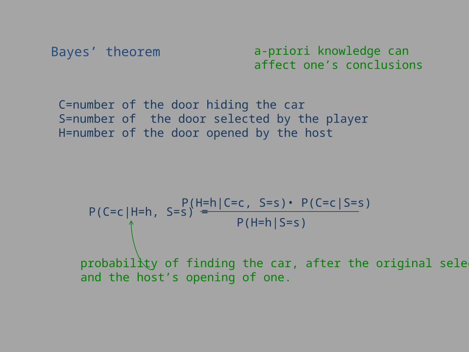
P(C=c|H=h, S=s) = P(H=h|C=c, S=s)• P(C=c|S=s)
P(H=h|S=s)
C=number of the door hiding the carS=number of the door selected by the playerH=number of the door opened by the host
probability of finding the car, after the original selectionand the host’s opening of one.
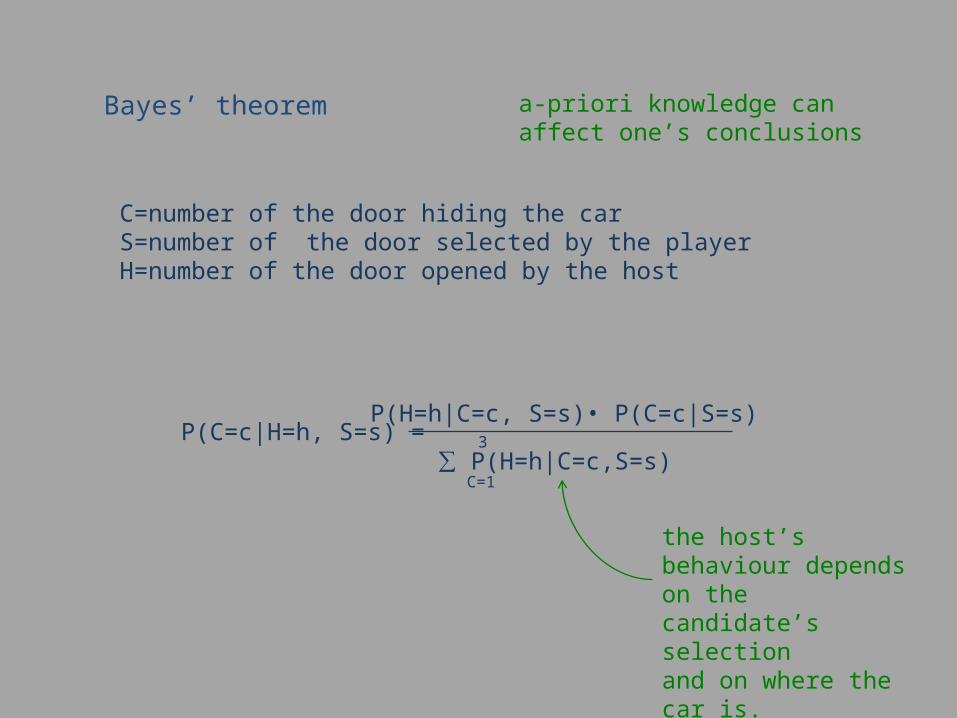
Bayes’ theorem a-priori knowledge can affect one’s conclusions
P(C=c|H=h, S=s) = P(H=h|C=c, S=s)• P(C=c|S=s)
∑ P(H=h|C=c,S=s)
C=number of the door hiding the carS=number of the door selected by the playerH=number of the door opened by the host
the host’s behaviour depends on the candidate’s selectionand on where the car is.
C=1
3
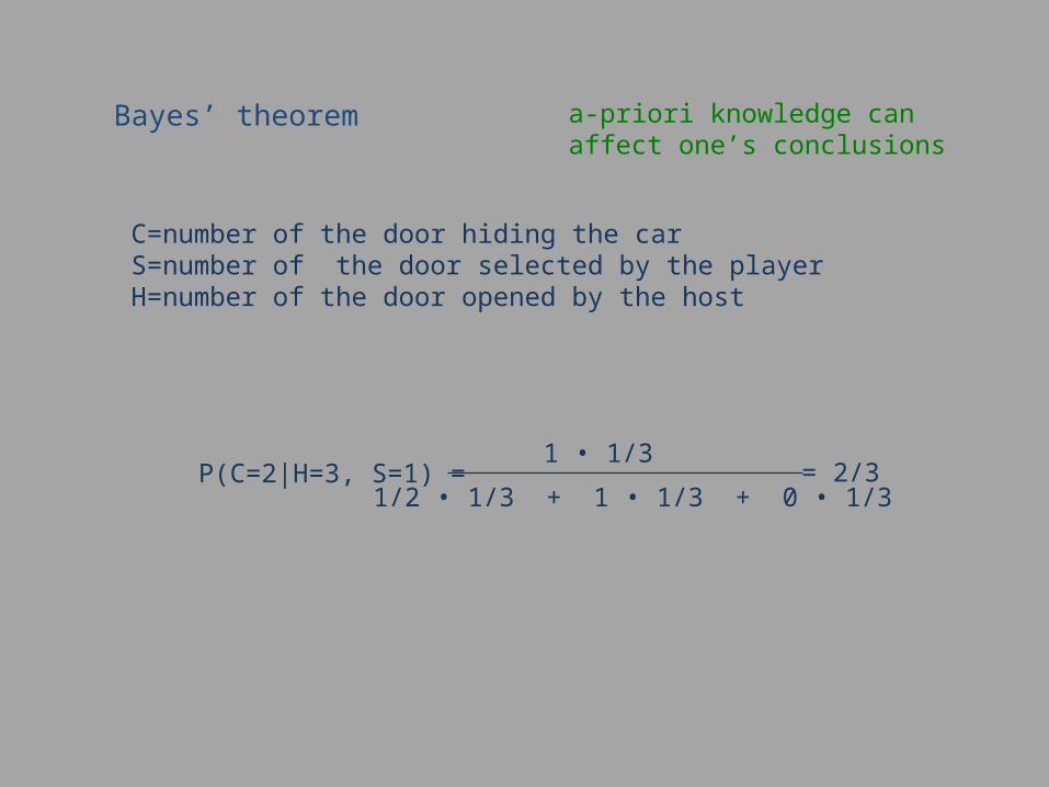
Bayes’ theorem a-priori knowledge can affect one’s conclusions
P(C=2|H=3, S=1) = 1 • 1/3
C=number of the door hiding the carS=number of the door selected by the playerH=number of the door opened by the host
1/2 • 1/3 + 1 • 1/3 + 0 • 1/3= 2/3
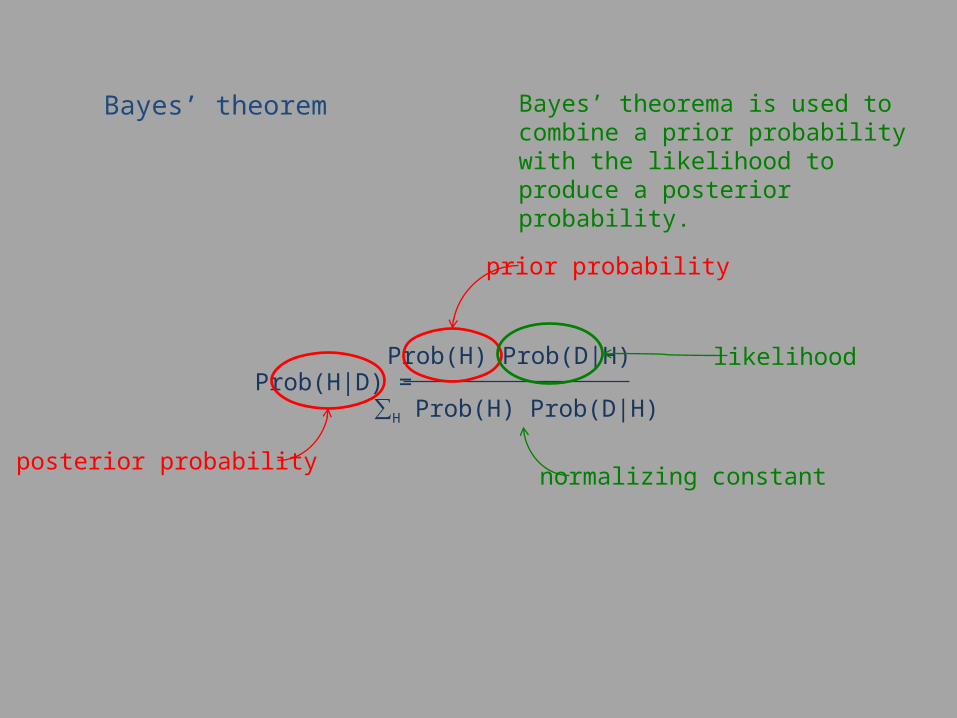
Bayes’ theorem Bayes’ theorema is used to combine a prior probability with the likelihood to produce a posterior probability.
Prob(H|D) = Prob(H) Prob(D|H)
∑H Prob(H) Prob(D|H)
prior probability
posterior probability
likelihood
normalizing constant
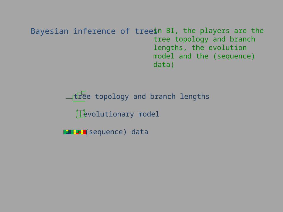
Bayesian inference of trees in BI, the players are the tree topology and branch lengths, the evolution model and the (sequence) data)
tree topology and branch lengths
evolutionary modelA G
C T
(sequence) data
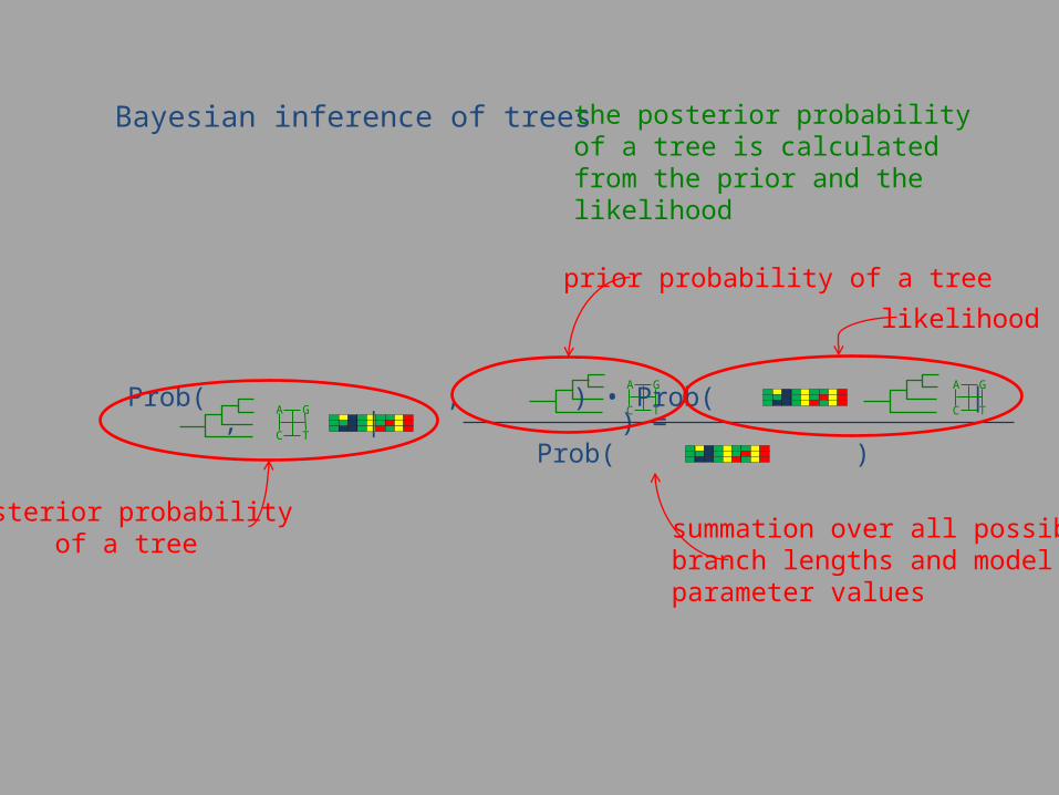
Bayesian inference of trees the posterior probability of a tree is calculated from the prior and the likelihood
A G
C TProb( , | ) =
A G
C TProb( , ) • Prob( | , )
A G
C T
Prob( )
posterior probabilityof a tree
prior probability of a tree
summation over all possible branch lengths and modelparameter values
likelihood
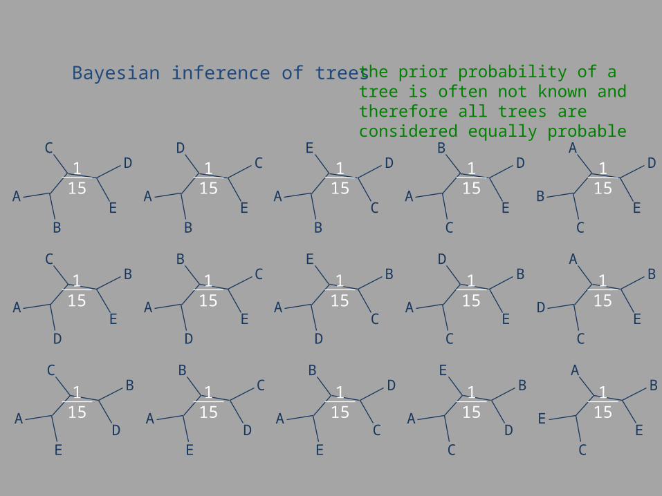
Bayesian inference of trees the prior probability of a tree is often not known and therefore all trees are considered equally probable
A
B
CD
EA
B
DC
EA
B
ED
CA
C
BD
EB
C
AD
E
A
D
CB
EA
D
BC
EA
D
EB
CA
C
DB
ED
C
AB
E
A
E
CB
DA
E
BC
DA
E
BD
CA
C
EB
DE
C
AB
E
115
115
115
115
115
115
115
115
115
115
115
115
115
115
115
Bayesian inference of trees
Prob
(Tre
e i)
Prob
(Dat
a |T
ree
i)Pr
ob(T
ree
i |D
ata)
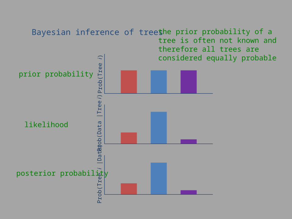
prior probability
likelihood
posterior probability
the prior probability of a tree is often not known and therefore all trees are considered equally probable
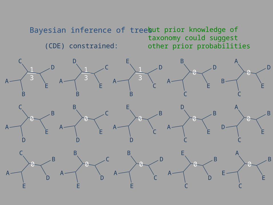
Bayesian inference of trees but prior knowledge of taxonomy could suggest other prior probabilities
A
B
CD
EA
B
DC
EA
B
ED
CA
C
BD
EB
C
AD
E
A
D
CB
EA
D
BC
EA
D
EB
CA
C
DB
ED
C
AB
E
A
E
CB
DA
E
BC
DA
E
BD
CA
C
EB
DE
C
AB
E
13
13
13
0 0
0 0 0
0 0 0 0 0
0 0
(CDE) constrained:
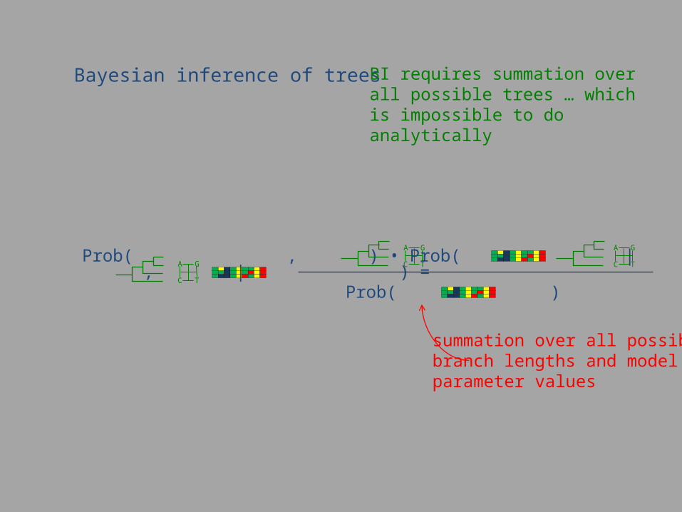
Bayesian inference of trees BI requires summation over all possible trees … which is impossible to do analytically
A G
C TProb( , | ) =
A G
C TProb( , ) • Prob( | , )
A G
C T
Prob( )
summation over all possible branch lengths and modelparameter values
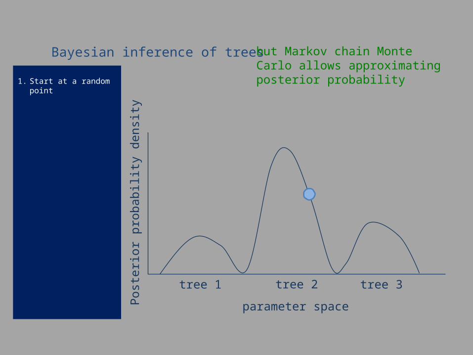
1. Start at a random point
Bayesian inference of trees but Markov chain Monte Carlo allows approximating posterior probability
Post
erio
r pro
babi
lity
dens
ity
tree 1 tree 2 tree 3
parameter space
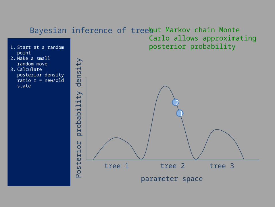
1. Start at a random point2. Make a small random
move3. Calculate posterior density
ratio r = new/old state
Bayesian inference of trees but Markov chain Monte Carlo allows approximating posterior probability
Post
erio
r pro
babi
lity
dens
ity
tree 1 tree 2 tree 3
parameter space
1
2
1. Start at a random point2. Make a small random
move3. Calculate posterior density
ratio r = new/old state4. If r > 1 always accept move
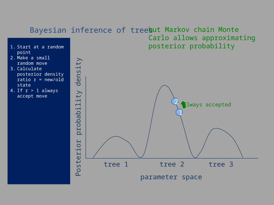
Bayesian inference of trees but Markov chain Monte Carlo allows approximating posterior probability
Post
erio
r pro
babi
lity
dens
ity
tree 1 tree 2 tree 3
parameter space
1
2 always accepted
1. Start at a random point2. Make a small random
move3. Calculate posterior density
ratio r = new/old state4. If r > 1 always accept move
If r < 1 accept move with a probability ~ 1/distance
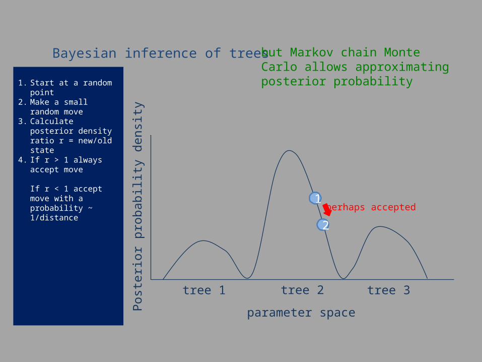
Bayesian inference of trees but Markov chain Monte Carlo allows approximating posterior probability
Post
erio
r pro
babi
lity
dens
ity
tree 1 tree 2 tree 3
parameter space
1
2
perhaps accepted
1. Start at a random point2. Make a small random
move3. Calculate posterior density
ratio r = new/old state4. If r > 1 always accept move
If r < 1 accept move with a probability ~ 1/distance
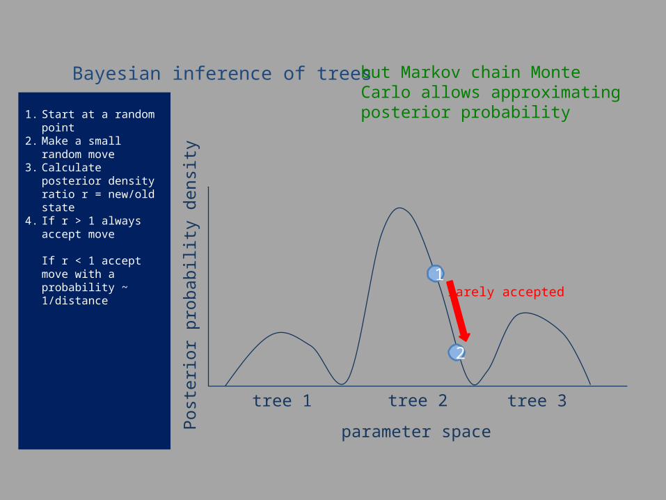
Bayesian inference of trees but Markov chain Monte Carlo allows approximating posterior probability
Post
erio
r pro
babi
lity
dens
ity
tree 1 tree 2 tree 3
parameter space
1
2
rarely accepted
1. Start at a random point2. Make a small random
move3. Calculate posterior density
ratio r = new/old state4. If r > 1 always accept move
If r < 1 accept move with a probability ~ 1/distance
5. Go to step 2
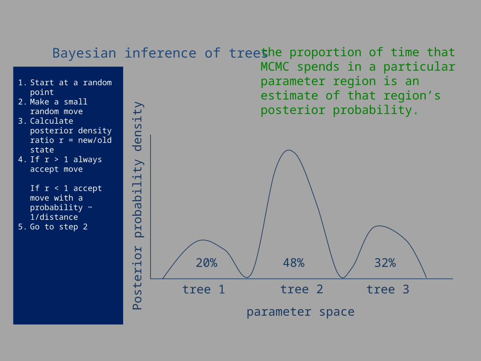
Bayesian inference of trees the proportion of time that MCMC spends in a particular parameter region is an estimate of that region’s posterior probability.
Post
erio
r pro
babi
lity
dens
ity
tree 1 tree 2 tree 3
parameter space
20% 48% 32%
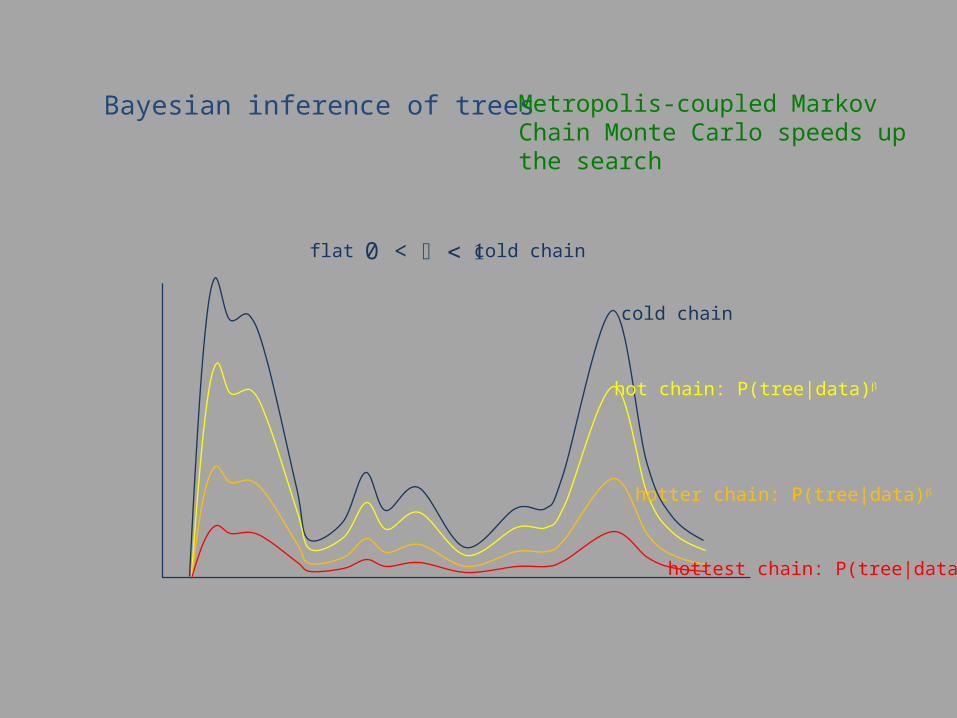
Bayesian inference of trees Metropolis-coupled Markov Chain Monte Carlo speeds up the search
cold chain
hot chain: P(tree|data)b
hotter chain: P(tree|data)b
hottest chain: P(tree|data)b
0 < < 1b cold chainflat
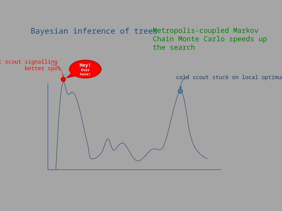
Bayesian inference of trees Metropolis-coupled Markov Chain Monte Carlo speeds up the search
cold scout stuck on local optimum
Hey!Over here!
hot scout signalling better spot