Embed Size (px)
Citation preview
Basis Functions for Serendipity Finite ElementMethods
Andrew Gillette
Department of MathematicsUniversity of California, San Diego
http://ccom.ucsd.edu/∼agillette/
14th International ConferenceApproximation Theory
Andrew Gillette - UCSD ( ) Serendipity FEM AT14 - Apr 2013 1 / 25

What is a serendipity finite element method?Goal: Efficient, accurate approximation of the solution to a PDE over Ω ⊂ Rn.Standard O(hr ) tensor product finite element method in Rn:→ Mesh Ω by n-dimensional cubes of side length h.→ Set up a linear system involving (r + 1)n degrees of freedom (DoFs) per cube.→ For unknown continuous solution u and computed discrete approximation uh:
||u − uh||H1(Ω)︸ ︷︷ ︸approximation error
≤ C hr |u|Hr+1(Ω)︸ ︷︷ ︸optimal error bound
, ∀u ∈ H r+1(Ω).
A O(hr ) serendipity FEM converges at the same rate with fewer DoFs per element:O(h) O(h2) O(h3) O(h) O(h2) O(h3)
tensorproduct
elements
serendipityelements
Example: For O(h3), d = 3, 50% fewer DoFs→ ≈ 50% smaller linear system
Andrew Gillette - UCSD ( ) Serendipity FEM AT14 - Apr 2013 2 / 25
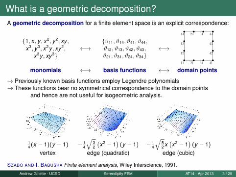
What is a geometric decomposition?A geometric decomposition for a finite element space is an explicit correspondence:
11 21 31 41
12 42
13 43
2414 34 44
1, x , y , x2, y2, xy ,x3, y3, x2y , xy2,
x3y , xy3←→
ϑ11, ϑ14, ϑ41, ϑ44,ϑ12, ϑ13, ϑ42, ϑ43,ϑ21, ϑ31, ϑ24, ϑ34
←→
monomials ←→ basis functions ←→ domain points
→ Previously known basis functions employ Legendre polynomials→ These functions bear no symmetrical correspondence to the domain points
and hence are not useful for isogeometric analysis.
14 (x − 1)(y − 1) − 1
4
√32
(x2 − 1
)(y − 1) − 1
4
√52 x(x2 − 1
)(y − 1)
vertex edge (quadratic) edge (cubic)
SZABÓ AND I. BABUŠKA Finite element analysis, Wiley Interscience, 1991.
Andrew Gillette - UCSD ( ) Serendipity FEM AT14 - Apr 2013 3 / 25

Motivations and Related Topics
Goal: Construct geometric decompositions of serendipity spaces using linearcombinations of standard tensor product functions. Focus: Cubic Hermites.
Isogeometric analysis: Finding basis functions suitable forboth domain description and PDE approximation avoids theexpensive computational bottleneck of re-meshing.COTTRELL, HUGHES, BAZILEVS Isogeometric Analysis:Toward Integration of CAD and FEA, Wiley, 2009.
Modern mathematics: Finite Element Exterior Calculus,Discrete Exterior Calculus, Virtual Element Methods. . .ARNOLD, AWANOU The serendipity family of finite elements,Found. Comp. Math, 2011.DA VEIGA, BREZZI, CANGIANI, MANZINI, RUSSO BasicPrinciples of Virtual Element Methods, M3AS, 2013.
Flexible Domain Meshing: Serendipity type elements forVoronoi meshes provide computational benefits withoutneed of tensor product structure.RAND, G., BAJAJ Quadratic Serendipity Finite Elements onPolygons Using Generalized Barycentric Coordinates,Mathematics of Computation, in press.
Andrew Gillette - UCSD ( ) Serendipity FEM AT14 - Apr 2013 4 / 25

Table of Contents
1 The Cubic Case: Hermite Functions, Serendipity Spaces
2 Geometric Decompsitions of Cubic Serendipity Spaces
3 Applications and Future Directions
Andrew Gillette - UCSD ( ) Serendipity FEM AT14 - Apr 2013 5 / 25

Outline
1 The Cubic Case: Hermite Functions, Serendipity Spaces
2 Geometric Decompsitions of Cubic Serendipity Spaces
3 Applications and Future Directions
Andrew Gillette - UCSD ( ) Serendipity FEM AT14 - Apr 2013 6 / 25

Cubic Hermite Geometric Decomposition: 1D
1 2 3 41, x , x2, x3 ←→ ψ1, ψ2, ψ3, ψ4 ←→
approxim. geometrymonomials ←→ basis functions ←→ domain points
CubicHermite Basis
on [0, 1]
ψ1
ψ2
ψ3
ψ4
:=
1− 3x2 + 2x3
x − 2x2 + x3
x2 − x3
3x2 − 2x3
0.0 0.2 0.4 0.6 0.8 1.0
0.2
0.4
0.6
0.8
1.0
Approximation: x r =4∑
i=1
εr,iψi , for r = 0, 1, 2, 3, where [εr,i ] =
1 0 0 10 1 −1 10 0 −2 10 0 −3 1
Geometry: u = u(0)ψ1 + u′(0)ψ2 − u′(1)ψ3 + u(1)ψ4, ∀u ∈ P3([0, 1])︸ ︷︷ ︸
cubic polynomials
Andrew Gillette - UCSD ( ) Serendipity FEM AT14 - Apr 2013 7 / 25
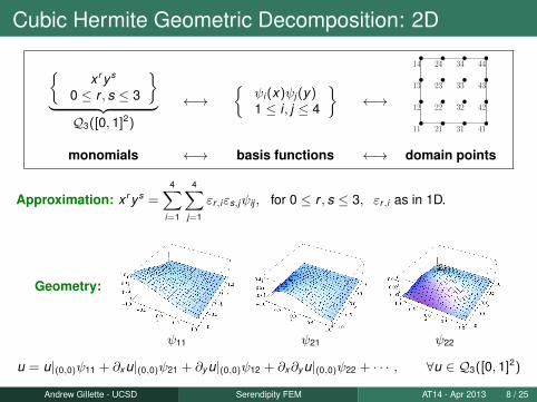
Cubic Hermite Geometric Decomposition: 2D
11 21 31 41
2212 32 42
2313 33 43
2414 34 44x r y s
0 ≤ r , s ≤ 3
︸ ︷︷ ︸Q3([0, 1]2)
←→
ψi (x)ψj (y)1 ≤ i, j ≤ 4
←→
monomials ←→ basis functions ←→ domain points
Approximation: x r y s =4∑
i=1
4∑j=1
εr,iεs,jψij , for 0 ≤ r , s ≤ 3, εr,i as in 1D.
Geometry:
ψ11 ψ21 ψ22
u = u|(0,0)ψ11 + ∂x u|(0,0)ψ21 + ∂y u|(0,0)ψ12 + ∂x∂y u|(0,0)ψ22 + · · · , ∀u ∈ Q3([0, 1]2)
Andrew Gillette - UCSD ( ) Serendipity FEM AT14 - Apr 2013 8 / 25
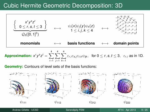
Cubic Hermite Geometric Decomposition: 3D
111 211
112 212
113 213
114 214
121
122
123
124
131
132
133
134
141
142
143
144
311
312
313
314
411
412
413
414
411
244 344 444
234 334 444
224 324 444x r y sz t
0 ≤ r , s, t ≤ 3
︸ ︷︷ ︸
Q3([0, 1]3)
←→ ψi (x)ψj (y)ψk (z)1 ≤ i, j, k ≤ 4 ←→
monomials ←→ basis functions ←→ domain points
Approximation: x r y sz t =4∑
i=1
4∑j=1
4∑k=1
εr,iεs,jεt,kψijk , for 0 ≤ r , s, t ≤ 3, εr,i as in 1D.
Geometry: Contours of level sets of the basis functions:
ψ111 ψ112 ψ212 ψ222
Andrew Gillette - UCSD ( ) Serendipity FEM AT14 - Apr 2013 9 / 25

Two families of finite elements on cubical meshesQ−r Λk ([0, 1]n) −→ tensor product spaces (≤ degree r in each variable)
early work: RAVIART, THOMAS 1976, NEDELEC 1980more recently: ARNOLD, BOFFI, BONIZZONI arXiv:1212.6559, 2012
Sr Λk ([0, 1]n) −→ serendipity finite element spaces (superlinear degree r )
early work: STRANG, FIX An analysis of the finite element method 1973more recently: ARNOLD, AWANOU FoCM 11:3, 2011, and arXiv:1204.2595, 2012.
The superlinear degree of a polynomial ignores linearly-appearing variables.
n = 2 :
Q3Λ0([0,1]2) (dim=16)︷ ︸︸ ︷1, x , y , x2, y2, xy , x3, y3, x2y , xy2, x3y , xy3︸ ︷︷ ︸
S3Λ0([0,1]2) (dim=12)
, x2y2, x3y2, x2y3, x3y3
n = 3 :
Q3Λ0([0,1]3) (dim=64)︷ ︸︸ ︷1, . . . , xyz, x3y , x3z, y3z, . . . , x3yz, xy3z, xyz3︸ ︷︷ ︸
S3Λ0([0,1]3) (dim=32)
, x3y2, . . . , x3y3z3
Q−r Λk and Sr Λk and have the same key mathematical properties needed for FEEC
(degree, inclusion, trace, subcomplex, unisolvence, commuting projections)but for fixed k ≥ 0, r , n ≥ 2 the serendipity spaces have fewer degrees of freedom
Andrew Gillette - UCSD ( ) Serendipity FEM AT14 - Apr 2013 10 / 25
Outline
1 The Cubic Case: Hermite Functions, Serendipity Spaces
2 Geometric Decompsitions of Cubic Serendipity Spaces
3 Applications and Future Directions
Andrew Gillette - UCSD ( ) Serendipity FEM AT14 - Apr 2013 11 / 25
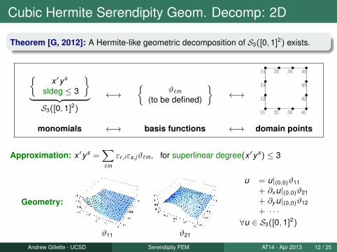
Cubic Hermite Serendipity Geom. Decomp: 2D
Theorem [G, 2012]: A Hermite-like geometric decomposition of S3([0, 1]2) exists.
11 21 31 41
12 42
13 43
2414 34 44x r y s
sldeg ≤ 3
︸ ︷︷ ︸S3([0, 1]2)
←→
ϑ`m
(to be defined)
←→
monomials ←→ basis functions ←→ domain points
Approximation: x r y s =∑`m
εr,iεs,jϑ`m, for superlinear degree(x r y s) ≤ 3
Geometry:
ϑ11 ϑ21
u = u|(0,0)ϑ11
+ ∂x u|(0,0)ϑ21
+ ∂y u|(0,0)ϑ12
+ · · ·∀u ∈ S3([0, 1]2)
Andrew Gillette - UCSD ( ) Serendipity FEM AT14 - Apr 2013 12 / 25
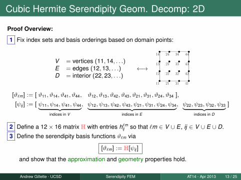
Cubic Hermite Serendipity Geom. Decomp: 2D
Proof Overview:
1 Fix index sets and basis orderings based on domain points:
11 21 31 41
2212 32 42
2313 33 43
2414 34 44
V = vertices (11, 14, . . .)E = edges (12, 13, . . .)D = interior (22, 23, . . .)
←→
[ϑ`m] := [ ϑ11, ϑ14, ϑ41, ϑ44, ϑ12, ϑ13, ϑ42, ϑ43, ϑ21, ϑ31, ϑ24, ϑ34 ],
[ψij ] := [ ψ11, ψ14, ψ41, ψ44︸ ︷︷ ︸indices in V
, ψ12, ψ13, ψ42, ψ43, ψ21, ψ31, ψ24, ψ34︸ ︷︷ ︸indices in E
, ψ22, ψ23, ψ32, ψ33︸ ︷︷ ︸indices in D
]
2 Define a 12× 16 matrix H with entries h`mij so that `m ∈ V ∪ E , ij ∈ V ∪ E ∪ D.
3 Define the serendipity basis functions ϑ`m via
[ϑ`m] := H[ψij ]
and show that the approximation and geometry properties hold.
Andrew Gillette - UCSD ( ) Serendipity FEM AT14 - Apr 2013 13 / 25

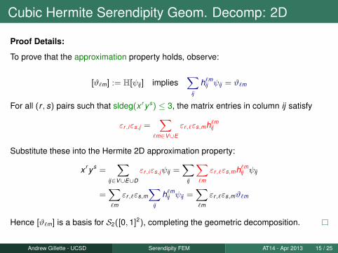
Cubic Hermite Serendipity Geom. Decomp: 2DProof Details:
2 Define a 12× 16 matrix H with entries h`mij so that `m ∈ V ∪ E , ij ∈ V ∪ E ∪ D.
H :=
I(12x12 identity matrix)
∣∣∣∣∣∣∣∣∣∣∣∣∣∣∣∣∣∣∣∣∣∣∣
−1 1 1 −11 −1 −1 11 −1 −1 1
−1 1 1 −1−1 0 1 0
0 −1 0 11 0 −1 00 1 0 −1
−1 1 0 00 0 −1 11 −1 0 00 0 1 −1
3 Define [ϑ`m] := H[ψij ]. The geometry property holds since for `m ∈ V ∪ E ,
ϑ`m = ψ`m︸︷︷︸bicubic Hermite
+∑ij∈D
h`mij ψij︸ ︷︷ ︸
zero on boundary
=⇒ ϑ`m ≡ ψ`m on edges
Andrew Gillette - UCSD ( ) Serendipity FEM AT14 - Apr 2013 14 / 25
Cubic Hermite Serendipity Geom. Decomp: 2D
Proof Details:
To prove that the approximation property holds, observe:
[ϑ`m] := H[ψij ] implies∑
ij
h`mij ψij = ϑ`m
For all (r , s) pairs such that sldeg(x r y s) ≤ 3, the matrix entries in column ij satisfy
εr,iεs,j =∑
`m∈V∪E
εr,`εs,mh`mij
Substitute these into the Hermite 2D approximation property:
x r y s =∑
ij∈V∪E∪D
εr,iεs,jψij =∑
ij
∑`m
εr,`εs,mh`mij ψij
=∑`m
εr,`εs,m
∑ij
h`mij ψij =
∑`m
εr,`εs,mϑ`m
Hence [ϑ`m] is a basis for S2([0, 1]2), completing the geometric decomposition.
Andrew Gillette - UCSD ( ) Serendipity FEM AT14 - Apr 2013 15 / 25

Hermite Style Serendipity Functions (2D)
[ϑ`m] =
ϑ11ϑ14ϑ41ϑ44ϑ12ϑ13ϑ42ϑ43ϑ21ϑ31ϑ24ϑ34
=
−(x − 1)(y − 1)(−2 + x + x2 + y + y2)(x − 1)(y + 1)(−2 + x + x2 − y + y2)(x + 1)(y − 1)(−2 − x + x2 + y + y2)−(x + 1)(y + 1)(−2 − x + x2 − y + y2)
−(x − 1)(y − 1)2(y + 1)(x − 1)(y − 1)(y + 1)2
(x + 1)(y − 1)2(y + 1)−(x + 1)(y − 1)(y + 1)2
−(x − 1)2(x + 1)(y − 1)(x − 1)(x + 1)2(y − 1)(x − 1)2(x + 1)(y + 1)−(x − 1)(x + 1)2(y + 1)
·18
ϑ11 ϑ21 ϑ31
Andrew Gillette - UCSD ( ) Serendipity FEM AT14 - Apr 2013 16 / 25
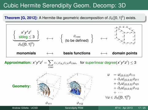
Cubic Hermite Serendipity Geom. Decomp: 3D
Theorem [G, 2012]: A Hermite-like geometric decomposition of S3([0, 1]3) exists.
111 211
112
113
114 214
121
124
131
134
141
142
143
144
311
314
411
412
413
414
411
244 344 444
444
444x r y sz t
sldeg ≤ 3
︸ ︷︷ ︸S3([0, 1]3)
←→
ϑ`mn
(to be defined)
←→
monomials ←→ basis functions ←→ domain points
Approximation: x r y sz t =∑`mn
εr,iεs,jεt,kϑ`mn, for superlinear degree(x r y sz t ) ≤ 3
Geometry:
ϑ111 ϑ112
u = u|(0,0,0)ϑ111
+ ∂x u|(0,0,0)ϑ211
+ ∂y u|(0,0,0)ϑ121
+ ∂zu|(0,0,0)ϑ112
+ · · ·∀u ∈ S3([0, 1]3)
Andrew Gillette - UCSD ( ) Serendipity FEM AT14 - Apr 2013 17 / 25

Cubic Hermite Serendipity Geom. Decomp: 3D
Proof Overview:
1 Fix index sets and basis orderings based on domain points:
111 211
112 212
113 213
114 214
121
122
123
124
131
132
133
134
141
142
143
144
311
312
313
314
411
412
413
414
411
244 344 444
234 334 444
224 324 444V = vertices (111, . . .)E = edges (112, . . .)F = face interior (122, . . .)M = volume interior (222, . . .)
←→
[ϑ`mn] := [ ϑ111, . . . , ϑ444, ϑ112, . . . , ϑ443 ],
[ψijk ] := [ ψ111, . . . , ψ444︸ ︷︷ ︸indices in V
, ψ112, . . . , ψ443︸ ︷︷ ︸indices in E
, ψ122, . . . , ψ433︸ ︷︷ ︸indices in F
, ψ222, . . . , ψ333︸ ︷︷ ︸indices in M
]
2 Define a 32× 64 matrix W with entries h`mnijk (where `mn ∈ V ∪ E)
3 Define the serendipity basis functions ϑ`mn via
[ϑ`mn] := W[ψijk ]
and show that the approximation and geometry properties hold.
Andrew Gillette - UCSD ( ) Serendipity FEM AT14 - Apr 2013 18 / 25
Cubic Hermite Serendipity Geom. Decomp: 3D
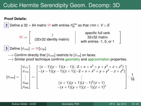
Proof Details:
2 Define a 32× 64 matrix W with entries h`mnijk so that `mn ∈ V ∪ E
W :=
I(32x32 identity matrix)
∣∣∣∣∣∣specific full rank
32x32 matrixwith entries -1, 0, or 1
3 Define [ϑ`mn] := W[ψijk ].
−→ Confirm directly that [ϑ`mn] restricts to [ϑ`m] on faces.−→ Similar proof technique confirms geometry and approximation properties.
[ϑ`mn] =
ϑ111
ϑ114...
ϑ442
ϑ443
=
(x − 1)(y − 1)(z − 1)(−2 + x + x2 + y + y2 + z + z2)
−(x − 1)(y − 1)(z + 1)(−2 + x + x2 + y + y2 − z + z2)...
(x + 1)(y + 1)(z − 1)2(z + 1)
−(x + 1)(y + 1)(z − 1)(z + 1)2
·1
16
Andrew Gillette - UCSD ( ) Serendipity FEM AT14 - Apr 2013 19 / 25
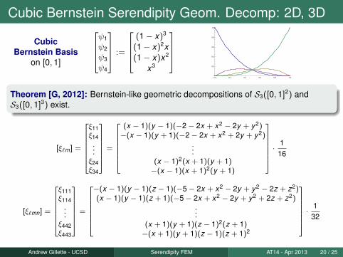
Cubic Bernstein Serendipity Geom. Decomp: 2D, 3D
CubicBernstein Basis
on [0, 1]
ψ1
ψ2
ψ3
ψ4
:=
(1− x)3
(1− x)2x(1− x)x2
x3
0.0 0.2 0.4 0.6 0.8 1.0
0.2
0.4
0.6
0.8
1.0
Theorem [G, 2012]: Bernstein-like geometric decompositions of S3([0, 1]2) andS3([0, 1]3) exist.
[ξ`m] =
ξ11ξ14...ξ24ξ34
=
(x − 1)(y − 1)(−2 − 2x + x2 − 2y + y2)−(x − 1)(y + 1)(−2 − 2x + x2 + 2y + y2)
...(x − 1)2(x + 1)(y + 1)−(x − 1)(x + 1)2(y + 1)
·1
16
[ξ`mn] =
ξ111ξ114
...ξ442ξ443
=
−(x − 1)(y − 1)(z − 1)(−5 − 2x + x2 − 2y + y2 − 2z + z2)(x − 1)(y − 1)(z + 1)(−5 − 2x + x2 − 2y + y2 + 2z + z2)
...(x + 1)(y + 1)(z − 1)2(z + 1)−(x + 1)(y + 1)(z − 1)(z + 1)2
·1
32
Andrew Gillette - UCSD ( ) Serendipity FEM AT14 - Apr 2013 20 / 25

Bernstein Style Serendipity Functions (2D)
β11 β21 β31
ξ11 ξ21 ξ31
0.0 0.2 0.4 0.6 0.8 1.0
0.2
0.4
0.6
0.8
1.0
Bicubic Bernstein functions (top) and Bernstein-styleserendipity functions (bottom).→ Note boundary agreement with Bernstein functions.
Andrew Gillette - UCSD ( ) Serendipity FEM AT14 - Apr 2013 21 / 25
Outline
1 The Cubic Case: Hermite Functions, Serendipity Spaces
2 Geometric Decompsitions of Cubic Serendipity Spaces
3 Applications and Future Directions
Andrew Gillette - UCSD ( ) Serendipity FEM AT14 - Apr 2013 22 / 25

Application: Cardiac Electrophysiology
→ Cubic Hermite serendipity functionsrecently incorporated into Continuitysoftware package for cardiacelectrophysiology models.
→ Used to solve the monodomainequations, a type of reaction-diffusionequation
→ Initial results show agreement ofserendipity and standard bicubics on abenchmark problem with a4x computational speedup in 3D.
→ Fast computation essential to clinicalapplications and ‘real time’ simulations
GONZALEZ, VINCENT, G., MCCULLOCH High Order Interpolation Methods in CardiacElectrophysiology Simulation, in preparation, 2013.
Andrew Gillette - UCSD ( ) Serendipity FEM AT14 - Apr 2013 23 / 25

Future Directions and Open Questions
→ Applications to problems using Bernstein tensor product bases
→ Analysis of the use of serendipity bases for geometric modeling
→ Construction of bases for Sr Λk ([0, 1]n) for
→ Higher order scalar cases (k = 0, r > 3, n = 2, 3)→ Higher form order cases (k > 0)
Andrew Gillette - UCSD ( ) Serendipity FEM AT14 - Apr 2013 24 / 25

AcknowledgmentsMatt Gonzalez UC San DiegoKevin Vincent UC San DiegoAndrew McCulloch UC San Diego
Michael Holst UC San DiegoNational Biomedical Computation Resource UC San Diego
Thanks to the NSF and conference organizers for travel support!
Slides and pre-prints: http://ccom.ucsd.edu/~agillette
Andrew Gillette - UCSD ( ) Serendipity FEM AT14 - Apr 2013 25 / 25