Basilar membrane motion to two Imagine the cochlea

Cochlea & Auditory Nerve:obligatory stages of auditory processing

Think of the auditory periphery as a processor of signals

-5

0

5

10

15

20

25

100 1000 10000-5

0

5

10

15

20

25

100 1000 10000

Imagine the cochlea unrolledBasilar membrane motion to two sinusoids of different frequency

Defining the envelope of the travelling wave

A crucial distinctionexcitation pattern vs. frequency response

• Excitation pattern — the vibration pattern across the basilar membrane to a single sound.– Input = 1 sound.

– Measure at many places along the BM.

• Essentially the envelope of the travelling wave

• Related to a spectrum (amplitude by frequency).• Related to a spectrum (amplitude by frequency).

A crucial distinctionexcitation pattern vs. frequency response

• Frequency response — the amount of vibration shown by a particular place on the BM to sinusoids of varying frequency.– Input = many sinusoids.– Measure at a single place on the BM.– Band-pass filters at each position along the basilar membrane.

– Band-pass filters at each position along the basilar membrane.

Two sides of the same coin:Deriving excitation patterns for a 1 kHz

sinusoid from frequency responses

Note shallower slope to lower frequencies (left) for frequency responses

300 Hz frequency 1900 Hz

Frequency responses with centre frequenciesrunning from 1400 – 600 Hz

1400 Hz

Frequency responses with centre frequenciesrunning from 1400 – 600 Hz

Deriving excitation pattern from auditory filters

Note shallower slope to left

Note shallower slope to right

Now the other way around:filter shapes from excitation patterns

base apex

high frequencies low


Flip the orientation of the axis and schematise

apex base

low frequencies high


The other side of the coin:Deriving a frequency response at 1 kHz

from excitation patterns

Note shallower slope to higher frequencies (right) for excitation patterns

300 Hz frequency 1900 Hz

Excitation patterns with centre frequenciesrunning from 1200 – 400 Hz

1200 Hz

Excitation patterns with centre frequenciesrunning from 1200 – 400 Hz

1200 Hz

Deriving frequency responses from excitation patterns



Laser Doppler Velocimetry

http://www.wadalab.mech.tohoku.ac.jp/bmldv-e.html

Modern measure-

ments of the frequency response of the basilar membranemembrane

Consider the frequency

response of a single placeon the BM

input/ output

functions on the on the basilar

membrane

Waveform of response to clicks on the basilar membrane (a.k.a. ?)

CF= 14.5 kHzClick

responses at various at various BM places

CF = 14.5 kHz CF = 5.5 kHz

What else can you do to impulse impulse responses(and why)?

Innervation of the cochlea

90-95% of afferents are myelinated, synapsing with a single inner hair cell (IHC).

Four aspects of firing patterns on the auditory nerve

• The coding of intensity.

• The representation of the place code.code.

• The representation of temporal fine structure (for intervals ranging up to ≈20 ms).

• The representation of gross temporal structure.

Intensity

Rate-level functions for auditory nerve auditory nerve

fibres

Observe!

• Threshold

• Saturation

• Limited dynamic range

However, firing rates depend not only on sinusoidal sound

intensity but also on intensity but also on sound ...

Firing rate across frequency and level ‘Audiograms’ of single auditory nerve fibres reflect BM tuning

The ‘best’ frequency of a particular tuning curve depends upon the BM position of the IHC to which the afferent

neuron is synapsing

BM and neural tuning compared

‘filtered’ is high-pass filter at 3.8 dB/octave. From Ruggero et al. 2000

Information about stimulus frequency is not only coded by which nerve fibres are active

Temporal coding (up to ≈ 5 kHz)

which nerve fibres are active (the place code) but also by when the fibres fire (the time

code).

The firing of auditory nerve fibres is synchronized to movements of the hair cell cilia (at low enough frequencies)

Play transdct.mov

Auditory nerves tend to fire to low-frequency sounds at particular waveform times (phase locking).

Evans (1975)

Not the same as firing rate!

But phase-locking is limited to lower frequencies ...

• Synchrony of neural firing is strong up to about 1-2 kHz.

• There is no evidence of synchrony • There is no evidence of synchrony above 5 kHz.

• The degree of synchrony decreases steadily over the mid-frequency range.

… as readily seen in a period histogram

Period histograms across frequency

Note half-wave rectification and synchrony index

Constructing an interval histogram

t1 t7t5t3

t8t6t4t2

Interval histograms for a single AN fibre at

Number o

f intervals per b

in

AN fibre at two

different frequencies

Number o

f intervals per b

in

0 5 10 15 20time (ms)

Interval histograms for a single AN fibre AN fibre across

frequency

Neural stimulation to a low frequency tone

Sound energy propagates to the characteristic place of the tone where it causes deflection of the cochlear partition. Neural spikes, when they occur, are synchronized to the peaks of the local deflections. The sum of these neural spikes tends to mimic the wave shape of the local deflections.

Period histograms to more complex sounds

Gross temporal structureEnhanced response to sound onsets:

The value of novelty

PST (Peri-Stimulus Time) histogram

Where we’ve got to …

• Outer ear channels sound to the middle ear, and can be characterized as a bandpass filter.

• Middle ear effects an efficient transfer of sound energy into the inner ear, again with the characteristics of a bandpass filter.

• Inner ear– Transduces basilar membrane movements into nerve firings …

– which are synchronised to peaks in the stimulating waveform at low enough frequencies

– Performs a mechanical frequency analysis, which can be envisioned as the result of analysis by a filter bank.

Auditory Nerve Structure and Function

Cochlea

Tuning curves

CochlearFrequencyMap

Liberman (1982)

Single-unitRecordingElectrode

Auditory Nerve

Tracer

Apex

Base

A systems model of the auditory periphery

-5

0

5

10

15

20

25

100 1000 10000-5

0

5

10

15

20

25

100 1000 10000

What properties should the filter bank have?

• Filter spacing

–Corresponding to tonotopic map

• Filter bandwidth

–vary with frequency as on the basilar –vary with frequency as on the basilar membrane

• Filter nonlinearity

–vary gain and bandwidth with level as on the basilar membrane

Modelling the hair cell/auditory nerve synapse

• Neuro-transmitter is released when cilia are pushed in one direction

period histogramsdirection only, tied to polarity of basilar membrane motion– half-wave rectification


Phase-locking is limited to low

period histograms across frequency

low frequencies

– low-pass filtering

Input sinusoids

0.5 kHz

1.0 kHz

2.0 kHz

4.0 kHz

8.0 kHz

Half-wave rectification

0.5 kHz

1.0 kHz

2.0 kHz

4.0 kHz

8.0 kHz

Smoothing

0.5 kHz

1.0 kHz

strong synchrony

2.0 kHz

4.0 kHz

8.0 kHz

weak synchrony

no synchrony


• Rapid adaptation

–need –need some kind of automatic gain control (agc)

Neural stimulation to a low frequency tone

We’re done!(but need agc here)

-5

0

5

10

15

20

25

100 1000 10000-5

0

5

10

15

20

25

100 1000 10000

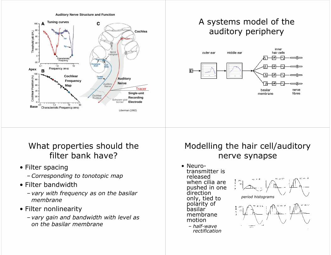
A spectrogram with ‘ear-like’ processing (Giguere & Woodland, 1993)

(typical spectrogram properties in italics)

• A first-stage broad band-pass linear filter to mimic outer and middle ear effects (pre-emphasis filter).

• A filterbank whose centre frequencies are arranged in the same way as the human tonotopic (frequency to place) map ... (equal tonotopic (frequency to place) map ... (equal spacing of filters in Hz).

• with non-linear filters whose bandwidths increase as level increases (linear filters with a fixed bandwoidth).

• Smearing of temporal information so as to mimic the frequency limitation of phase locking in the auditory nerve (smearing by choice of temporal window/filter bandwidth —no extra processing ).

An auditory spectrogram Types of Spectrogram

Wide-band Narrow-band Auditory

An auditory spectrogram looks like a wide-band spectrogram at high frequencies and a narrow-band spectrogram at low frequencies (but with more temporal structure).

Next lab: A computer implementation of essentially

this model

-5

0

5

10

15

20

25

100 1000 10000-5

0

5

10

15

20

25

100 1000 10000

A cochlear simulation

Flip it around

???

5

10

15

20

25

5

10

15

20

25

??

-5

0

100 1000 10000-5

0

5

100 1000 10000

A cochlear simulation

2525

-5

0

5

10

15

20

100 1000 10000-5

0

5

10

15

20

25

100 1000 10000

How should we look at the output of the model?

Could look at the output waveforms

input signal

-5

0

5

10

15

20

25

100 1000 10000-5

0

5

10

15

20

25

100 1000 10000

output signal

But hard to see what is going on (especially for complex waves)

Solution: encode wave amplitude in a different way

waveform at 200 Hz

rectified & smoothedrectified & smoothed

spectrographic

waveform amplitude is recoded as the darkness of the trace

Encode wave amplitude as trace darkness

waveform at 1 kHz


spectrographic

Encode wave amplitude as trace darkness

waveform at 4 kHz


spectrographic

Construct the output display one strip at a time

input signal at 200 Hz

-5

0

5

10

15

20

25

100 1000 10000-5

0

5

10

15

20

25

100 1000 10000

output display

Construct the output display one strip at a time

input signal at 4 kHz

-5

0

5

10

15

20

25

100 1000 10000-5

0

5

10

15

20

25

100 1000 10000

output display

4 kHz + 200 Hz

input signal

-5

0

5

10

15

20

25

100 1000 10000-5

0

5

10

15

20

25

100 1000 10000

output display

4 kHz + 200 Hz Auditory and ordinary spectrograms

Documents

Basilar membrane motion to two Imagine the cochlea