Basic Principles of SAR Polarimetry 1

Basic Principles of SAR Polarimetry 1C. López-Martínez and E. Pottier

Abstract

This chapter critically summarizes the main theoreticalaspects necessary for a correct processing and interpreta-tion of the polarimetric information towards the develop-ment of applications of synthetic aperture radar (SAR)polarimetry. First of all, the basic principles of wavepolarimetry (which deals with the representation and theunderstanding of the polarization state of an electromag-netic wave) and scattering polarimetry (which concernsinferring the properties of a target given the incident andthe scattered polarized electromagnetic waves) are given.Then, concepts regarding the description of polarimetricdata are reviewed, covering statistical and scatteringaspects, the latter in terms of coherent and incoherentdecomposition techniques. Finally, polarimetric SARinterferometry and tomography, two acquisition modesthat enable the extraction of the 3-D scatterer positionand separation, respectively, and their polarimetric char-acterization, are described.

1.1 Theory of Radar Polarimetry

1.1.1 Wave Polarimetry

Polarimetry refers specifically to the vector nature of theelectromagnetic waves, whereas radar polarimetry is the sci-ence of acquiring, processing and analysing the polarizationstate of an electromagnetic wave in radar applications. Thissection summarizes the main theoretical aspects necessary fora correct processing and interpretation of the polarimetric

information. As a result, the first part presents the so-calledwave polarimetry that deals with the representation and theunderstanding of the polarization state of an electromagneticwave. The second part introduces the concept of scatteringpolarimetry. This concept collects the topic of inferring theproperties of a given target, from a polarimetric point of view,given the incident and the scattered polarized electromagneticwaves.

1.1.1.1 Electromagnetic Waves and WavePolarization Descriptors

The generation, the propagation and the interaction withmatter of the electric and the magnetic waves are governedby Maxwell’s equations (Balanis 1989). For an electromag-netic wave that is propagating in the bz direction, the realelectric wave can be decomposed into two orthogonalcomponents bx and by , admitting the following vectorformulation:

E!

z, tð Þ ¼Ex

Ey

Ez

264375 ¼

E0x cos ωt � kzþ δxð ÞE0y cos ωt � kzþ δy

� �0

264375 ð1:1Þ

which may be also considered in a complex form

E!

z, tð Þ ¼Ex

Ey

Ez

264375 ¼

E0xe jδx e�jkzejωt

E0ye jδy e�jkzejωt

0

264375, ð1:2Þ

where E0x and E0y are the amplitudes of the waves in eachcoordinate. The electric wave in (1.1) and (1.2) presents aharmonic time dependence of the type e jωt, where ω ¼ 2πf isthe angular frequency and f is the time frequency. The propa-gation direction of an electromagnetic wave is determined bythe propagation vector bk that in case of (1.1) and (1.2) isconsidered parallel to bz . The amplitude of the propagationvector is represented by k ¼ 2π/λ, where λ is the wavelength.

C. López-Martínez (*)Signal Theory and Communications Department, UniversitatPolitècnica de Catalunya , Barcelona, Spaine-mail: [email protected]

E. PottierInstitut d’Électronique et de Télécommunications de Rennes, Universityof Rennes-1, Rennes, France

# The Author(s) 2021I. Hajnsek, Y.-L. Desnos (eds.), Polarimetric Synthetic Aperture Radar, Remote Sensing and Digital Image Processing 25,https://doi.org/10.1007/978-3-030-56504-6_1

1

http://crossmark.crossref.org/dialog/?doi=10.1007/978-3-030-56504-6_1&domain=pdf

mailto:[email protected]

https://doi.org/10.1007/978-3-030-56504-6_1#DOI

Finally, δx and δy represent the wave phases in each compo-

nent. The magnetic wave H!

z, tð Þ can be also represented inthe same form.

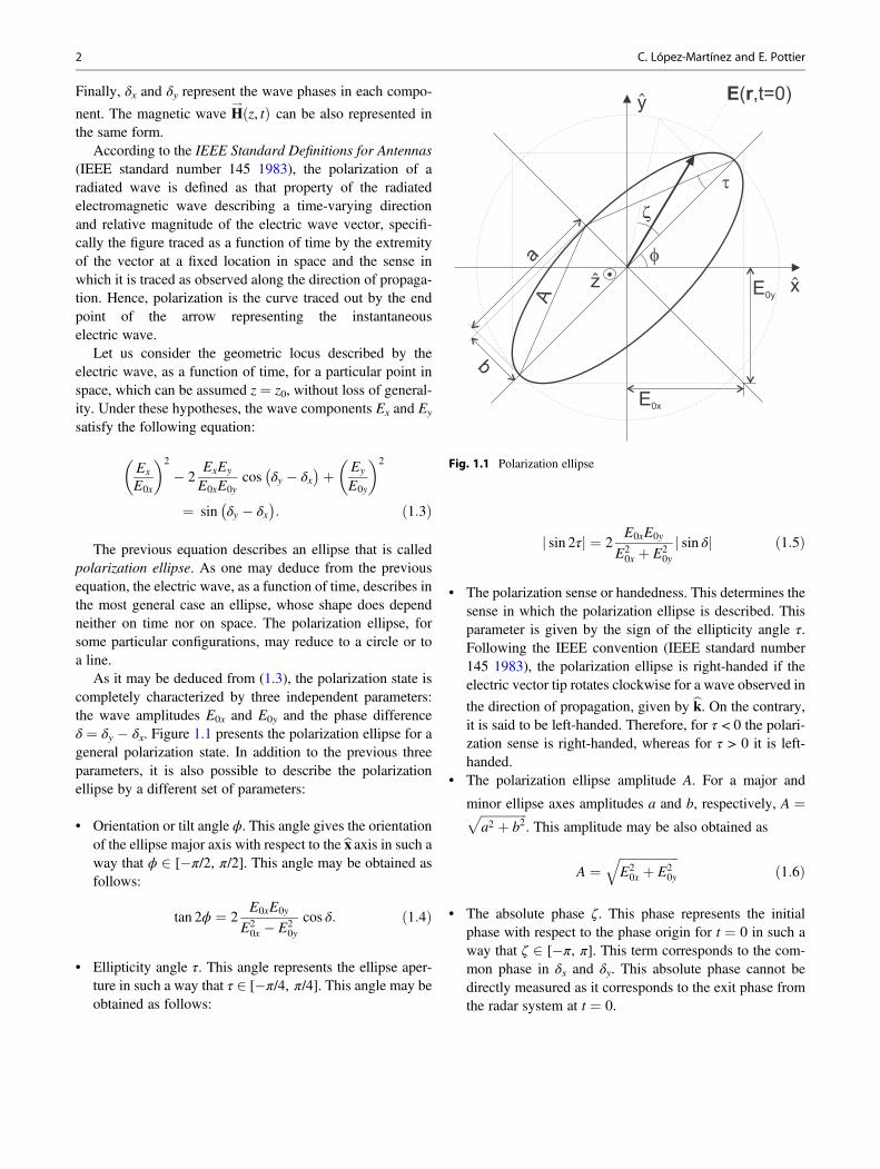
According to the IEEE Standard Definitions for Antennas(IEEE standard number 145 1983), the polarization of aradiated wave is defined as that property of the radiatedelectromagnetic wave describing a time-varying directionand relative magnitude of the electric wave vector, specifi-cally the figure traced as a function of time by the extremityof the vector at a fixed location in space and the sense inwhich it is traced as observed along the direction of propaga-tion. Hence, polarization is the curve traced out by the endpoint of the arrow representing the instantaneouselectric wave.

Let us consider the geometric locus described by theelectric wave, as a function of time, for a particular point inspace, which can be assumed z ¼ z0, without loss of general-ity. Under these hypotheses, the wave components Ex and Ey

satisfy the following equation:

Ex

E0x

� �2

� 2ExEy

E0xE0ycos δy � δx� �þ Ey

E0y

� �2

¼ sin δy � δx� �

: ð1:3Þ

The previous equation describes an ellipse that is calledpolarization ellipse. As one may deduce from the previousequation, the electric wave, as a function of time, describes inthe most general case an ellipse, whose shape does dependneither on time nor on space. The polarization ellipse, forsome particular configurations, may reduce to a circle or toa line.

As it may be deduced from (1.3), the polarization state iscompletely characterized by three independent parameters:the wave amplitudes E0x and E0y and the phase differenceδ ¼ δy � δx. Figure 1.1 presents the polarization ellipse for ageneral polarization state. In addition to the previous threeparameters, it is also possible to describe the polarizationellipse by a different set of parameters:

• Orientation or tilt angle ϕ. This angle gives the orientationof the ellipse major axis with respect to the bx axis in such away that ϕ 2 [�π/2, π/2]. This angle may be obtained asfollows:

tan 2ϕ ¼ 2E0xE0y

E20x � E2

0y

cos δ: ð1:4Þ

• Ellipticity angle τ. This angle represents the ellipse aper-ture in such a way that τ 2 [�π/4, π/4]. This angle may beobtained as follows:

sin 2τj j ¼ 2E0xE0y

E20x þ E2

0y

sin δj j ð1:5Þ

• The polarization sense or handedness. This determines thesense in which the polarization ellipse is described. Thisparameter is given by the sign of the ellipticity angle τ.Following the IEEE convention (IEEE standard number145 1983), the polarization ellipse is right-handed if theelectric vector tip rotates clockwise for a wave observed in

the direction of propagation, given by bk. On the contrary,it is said to be left-handed. Therefore, for τ < 0 the polari-zation sense is right-handed, whereas for τ > 0 it is left-handed.

• The polarization ellipse amplitude A. For a major and

minor ellipse axes amplitudes a and b, respectively, A ¼ffiffiffiffiffiffiffiffiffiffiffiffiffiffiffia2 þ b2

p. This amplitude may be also obtained as

A ¼ffiffiffiffiffiffiffiffiffiffiffiffiffiffiffiffiffiffiffiE20x þ E2

0y

qð1:6Þ

• The absolute phase ζ. This phase represents the initialphase with respect to the phase origin for t ¼ 0 in such away that ζ 2 [�π, π]. This term corresponds to the com-mon phase in δx and δy. This absolute phase cannot bedirectly measured as it corresponds to the exit phase fromthe radar system at t ¼ 0.

Fig. 1.1 Polarization ellipse

2 C. López-Martínez and E. Pottier

Considering the previous sets of parameters describing thepolarization state of a wave, one can identify some importantpolarization states that can be considered as canonical polari-zation states:

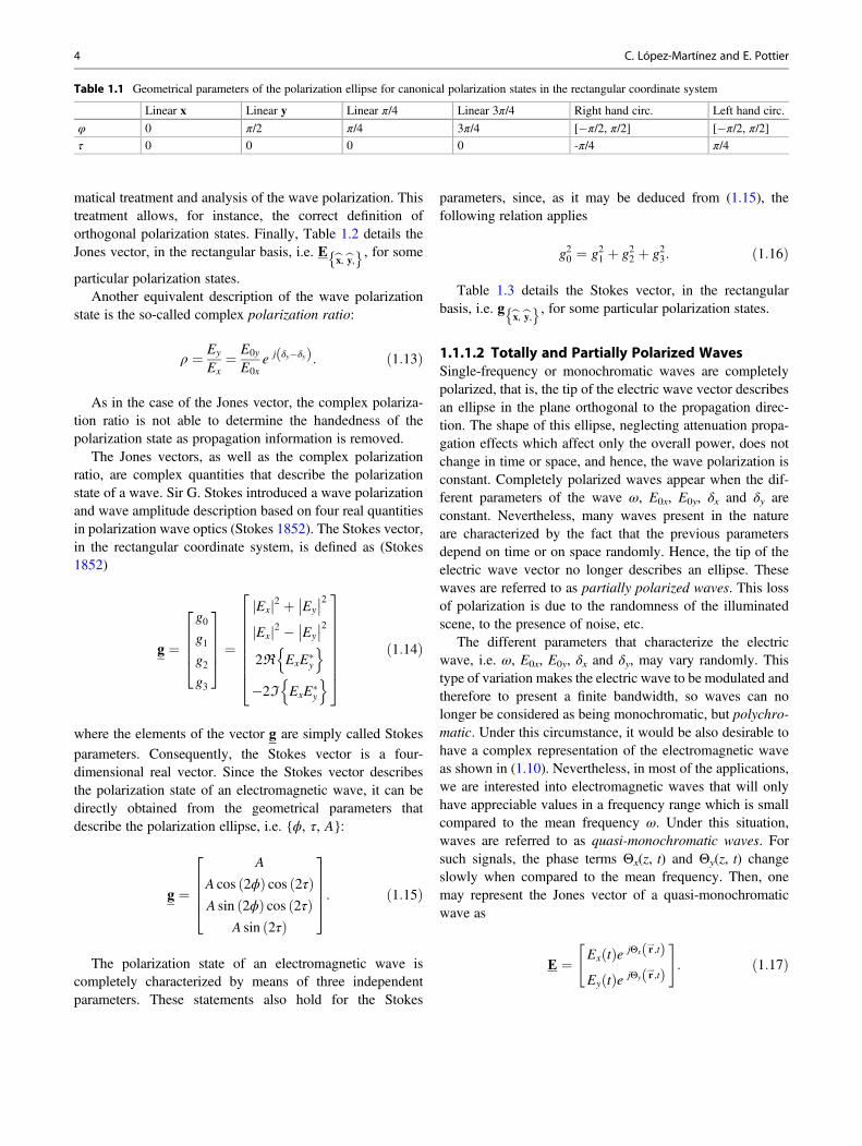
• Linear polarization state. Considering the expression forthe real electric wave in (1.1), two canonical linear polari-zation states can be identified. Table 1.1 details the orien-tation and the ellipticity angles for these polarizationstates. These are the linear polarization states accordingto the bx and to the by axes, respectively. The linear polari-zation states are characterized by presenting a phase dif-ference of

δ ¼ δy � δx ¼ mπ,m ¼ 0, � 1, � 2, . . . ð1:7Þ

As it may be seen, the linear nature of the polarizationstate is independent of the phase ζ.

• Circular polarization state. In this particular case, also twocanonical circular polarization states can be defined.Table 1.1 details the orientation and the ellipticity anglesfor these polarization states. When the ellipticity angletakes a value of �π/4, the circular polarization state isright-handed, whereas this value is equal to π/4 when it isleft-handed. The circular polarization states arecharacterized by presenting a phase difference of

δ ¼ δy � δx ¼ mπ2

m ¼ �1, � 3, � 5, . . . ð1:8Þ

and equal amplitudes for the components of the electric waveE0 ¼ E0x ¼ E0y. Also for circular polarization states, thepolarization state is independent of the absolute phase ζ.

• Elliptical polarization state. When there are notrestrictions on the orientation and ellipticity angle values,the electric wave is said to present an elliptical polariza-tion state.

As observed, the polarization ellipse may be completelydescribed by two equivalent sets of three independentparameters: the set of wave parameters {E0x, E0y, δ} or theset of ellipse parameters {ϕ, τ, A}. In addition to these, thereexist additional equivalent descriptors that are detailed in thefollowing.

Considering (1.1), the real electric wave vector can bedirectly obtained from the complex electric wave vector

E!

z,tð Þ¼E0xcos ωt�kzþδxð ÞE0ycos ωt�kzþδy

� �" #

¼ℜE0xe jδx

E0ye jδy

" #e�jkzejωt

( )¼

¼ℜ Ε!

zð Þejωtn o

ð1:9Þ

where ℜ{�} denotes the real part. The time dependence hasbeen removed from the wave description. This is possible asthe polarization state of the wave does not change with time.In order to derive a simple and concise description of thepolarization state, it is also possible to remove the space

dependence of Ε!

zð Þ by considering the polarization state ina particular point of the space. Without loss of generality, this

point can be z ¼ 0. Hence, Ε!

0ð Þ reduces to

E ¼ E!

0ð Þ ¼ E0xe jδx

E0ye jδy

" #: ð1:10Þ

The two-dimensional complex vector Ε is referred to asthe Jones vector, and it is a concise representation of amonochromatic, uniform plane wave with a constant polari-zation (Jones 1941a; Jones 1941b; Jones 1941c).

In the rectangular coordinate system, the Jones vector canbe written as a function of the parameters that describe thepolarization ellipse (Huynen 1970):

E ¼ Aejζcosϕ � sinϕ

sinϕ cosϕ

� �cos τ

j sin τ

� �: ð1:11Þ

The Jones vector, considering the unitary vectors bx and by,may be also expressed as

E bx,by, ¼ Acosϕ � sinϕ

sinϕ cosϕ

� �cos τ j sin τ

j sin τ cos τ

� �� ejζ 0

0 e�jζ

� �bx ð1:12Þ

where the sub-index bx, by,f g indicates that the Jones vector isexpressed in the linear basis bx, by,f g. The Jones vectordescribes completely the polarization ellipse shape, as wellas the rotation sense of the electric wave vector. On thecontrary, handedness information cannot be included withinthe Jones vector as propagation information has beenremoved. The use of the Jones vector to describe the polari-zation state is of enormous importance as it allows to define apolarization algebra that makes possible to perform a mathe-

1 Basic Principles of SAR Polarimetry 3

matical treatment and analysis of the wave polarization. Thistreatment allows, for instance, the correct definition oforthogonal polarization states. Finally, Table 1.2 details theJones vector, in the rectangular basis, i.e. E bx,by, , for some

particular polarization states.Another equivalent description of the wave polarization

state is the so-called complex polarization ratio:

ρ ¼ Ey

Ex¼ E0y

E0xe j δy�δyð Þ: ð1:13Þ

As in the case of the Jones vector, the complex polariza-tion ratio is not able to determine the handedness of thepolarization state as propagation information is removed.

The Jones vectors, as well as the complex polarizationratio, are complex quantities that describe the polarizationstate of a wave. Sir G. Stokes introduced a wave polarizationand wave amplitude description based on four real quantitiesin polarization wave optics (Stokes 1852). The Stokes vector,in the rectangular coordinate system, is defined as (Stokes1852)

g ¼

g0g1g2g3

2666437775 ¼

Exj j2 þ Ey

�� 2Exj j2 � Ey

�� 22ℜ ExE�

y

n o�2ℑ ExE�

y

n o

266666664

377777775 ð1:14Þ

where the elements of the vector g are simply called Stokes

parameters. Consequently, the Stokes vector is a four-dimensional real vector. Since the Stokes vector describesthe polarization state of an electromagnetic wave, it can bedirectly obtained from the geometrical parameters thatdescribe the polarization ellipse, i.e. {ϕ, τ, A}:

g ¼

A

A cos 2ϕð Þ cos 2τð ÞA sin 2ϕð Þ cos 2τð Þ

A sin 2τð Þ

2666437775: ð1:15Þ

The polarization state of an electromagnetic wave iscompletely characterized by means of three independentparameters. These statements also hold for the Stokes

parameters, since, as it may be deduced from (1.15), thefollowing relation applies

g20 ¼ g21 þ g22 þ g23: ð1:16Þ

Table 1.3 details the Stokes vector, in the rectangularbasis, i.e. g bx,by, , for some particular polarization states.

1.1.1.2 Totally and Partially Polarized WavesSingle-frequency or monochromatic waves are completelypolarized, that is, the tip of the electric wave vector describesan ellipse in the plane orthogonal to the propagation direc-tion. The shape of this ellipse, neglecting attenuation propa-gation effects which affect only the overall power, does notchange in time or space, and hence, the wave polarization isconstant. Completely polarized waves appear when the dif-ferent parameters of the wave ω, E0x, E0y, δx and δy areconstant. Nevertheless, many waves present in the natureare characterized by the fact that the previous parametersdepend on time or on space randomly. Hence, the tip of theelectric wave vector no longer describes an ellipse. Thesewaves are referred to as partially polarized waves. This lossof polarization is due to the randomness of the illuminatedscene, to the presence of noise, etc.

The different parameters that characterize the electricwave, i.e. ω, E0x, E0y, δx and δy, may vary randomly. Thistype of variation makes the electric wave to be modulated andtherefore to present a finite bandwidth, so waves can nolonger be considered as being monochromatic, but polychro-matic. Under this circumstance, it would be also desirable tohave a complex representation of the electromagnetic waveas shown in (1.10). Nevertheless, in most of the applications,we are interested into electromagnetic waves that will onlyhave appreciable values in a frequency range which is smallcompared to the mean frequency ω. Under this situation,waves are referred to as quasi-monochromatic waves. Forsuch signals, the phase terms Θx(z, t) and Θy(z, t) changeslowly when compared to the mean frequency. Then, onemay represent the Jones vector of a quasi-monochromaticwave as

Ε ¼ Ex tð Þe jΘx r!,tð Þ

Ey tð Þe jΘy r!,tð Þ

" #: ð1:17Þ

Table 1.1 Geometrical parameters of the polarization ellipse for canonical polarization states in the rectangular coordinate system

Linear x Linear y Linear π/4 Linear 3π/4 Right hand circ. Left hand circ.

φ 0 π/2 π/4 3π/4 [�π/2, π/2] [�π/2, π/2]

τ 0 0 0 0 -π/4 π/4


As one may see, the Jones vector of a quasi-monochromatic electric wave depends on time and onspace; thus, this vector is no longer constant. When the timedependence of the Jones vector is deterministic, the polari-metric properties of the wave also change in a deterministicway through time. In this case, the description of the wavepolarization is not problematic and may be performed con-sidering the different descriptors detailed in Sect. 1.1.1.1.Nevertheless, if the time dependence is random, the analysisof the polarization state of the electromagnetic wave must becarefully addressed, as this description must take into accountthe stochastic nature of the electric wave.

As previously mentioned, the variation of the parametersE0x, E0y, δx and δymay be random, so the Jones vector will bealso random. In order to characterize the polarization of thequasi-monochromatic electromagnetic wave expressed bythe variable Jones vector in (1.17), it is necessary to addressthis characterization from a stochastic point of view. In theframe of radar remote sensing, the wave transmitted by theradar system may be considered monochromatic and hencetotally polarized. Nevertheless, the scattered waverepresented by the Jones vector in (1.17) results from thecombination of many different waves originated by the dif-ferent elementary scatterers that form the scattering media.The complex addition of these elementary waves resultingfrom the scattering process for one component of the electricwave can be represented as

Aejθ ¼ 1ffiffiffiffiN

pXNn¼1

anejθn ð1:18Þ

where A represents the total wave and ane jθn is originatedfrom the scattering from every elementary scatterer. Underthe assumption of N, i.e. the total number of scattered waves,to be large enough and certain relations that may beestablished between the amplitude and the phase of the ele-mentary waves (Chandrasekhar 1960; Goodman 1976), it ispossible to demonstrate that the mean value of the electricwave and the Jones vector are zero. Consequently, the Jonesvector cannot be employed to characterize the polarization

state of a quasi-monochromatic wave. This characterizationshall be performed considering higher statistical moments.

The second-order moments may be arranged in a vectorform, giving rise to the so-called coherency vector of a quasi-monochromatic vector, which is defined in the followingway:

J ¼ E ΕO

Ε�n o

¼

E ExE�x

E ExE�

y

n oE EyE�

x

E EyE�

y

n o

26666664

37777775 ¼

Jxx

JxyJyxJyy

2666437775 ð1:19Þ

where J stands for the temporal averaging, assuming thewave is stationary,

Nis the Kronecker product, (�)�

represents complex conjugation and E{�} is the ensembleaverage. This vector is not zero for quasi-monochromaticwaves. The arrangement of the second-order moments canbe also done in a matrix, giving rise to the coherency matrixof the wave:

J ¼ E Ε � ΕT� ¼E ExE�

x

E ExE�

y

n oE EyE�

x

E EyE�

y

n o264

375¼ Jxx Jxy

Jyx Jyy

� �ð1:20Þ

where the superscript (�)T denotes vector transposition.In the previous section, it was mentioned that monochro-

matic waves are completely polarized. This is not the case forquasi-monochromatic waves. Indeed, completely polarizedwaves present a polarization state that can be considered asa limit in the sense that it is constant. The opposed extreme isa completely unpolarized wave for which the polarizationstate is completely random. Between both extremes, wavesare said to present a partial polarization state. In order tocharacterize the degree of polarization, one may considerthe degree of polarization defined as a function of the traceof matrix J as

Table 1.2 Jones vector for some polarization states in the rectangular coordinate system, for A ¼ 1


E bx,by 1

0

� �0

1

� �1ffiffi2

p1

1

� �1ffiffi2

p1

�1

� �1ffiffi2

p1

�j

� �1ffiffi2

p1

j

� �

Table 1.3 Stokes vector for some polarization states in the rectangular coordinate system, for A ¼ 1


g bx,by 1

1

0

0

2666437775

1

�1

0

0

2666437775

1

0

1

0

2666437775

1

0

�1

0

2666437775

1

0

0

�1

2666437775

1

0

0

1

2666437775


DoP ¼ 1� 4Jj j

trace Jð Þ� �1

2

: ð1:21Þ

1.1.1.3 Change of Polarization BasisAs seen in Sect. 1.1.1.1, an electromagnetic wave, consider-ing the coordinate system bx, by, bzf g, that propagates in bzmaybe decomposed as the sum of two orthogonal components.Separately, the electromagnetic wave of each component canbe considered as linearly polarized. Therefore, it is possibleto consider that the total electromagnetic wave results fromthe sum of two orthogonal linear polarized waves. Indeed,this representation must be extended in the sense that anyelectromagnetic wave propagating in an infinite, lossless,isotropic media can be decomposed as the sum of two orthog-onal elliptically polarized waves. The advantage of this rep-resentation is that the electric wave is decomposed in a pair oforthogonal polarization states, so it is possible, through adeterministic transformation, to obtain the electric wave forany other pair of orthogonal polarization states. This processis referred to as change of polarization basis or polarizationsynthesis.

Given two vectors a and b, they are considered orthogonalif they verify

a, bh i ¼ aT � b� ¼ 0 ð1:22Þ

that is, the scalar (Hermitian) product of both vectors is zero.In case of two electromagnetic waves, expressed in terms ofthe corresponding Jones vectors, they are said to be orthogo-nal if the scalar product of the Jones vectors is zero, consid-ering that both Jones vectors refer to waves propagating inthe same direction and sense. The polarization ellipsescorresponding to two orthogonal Jones vectors presents thesame ellipticity angle, opposite polarization sense and mutu-ally orthogonal polarization axis. That is, for a Jones vectorrepresenting a polarization state characterized by an orienta-tion angle ϕ, an ellipticity angle τ and an absolute phase ζ, itsorthogonal Jones vector presents an orientation angle ofvalue ϕ + π, an ellipticity angle of value �τ and an absolutephase �ζ. In terms of (1.12), the corresponding orthogonalvector is

E⊥ bx,by, ¼A

�sinϕ �cosϕ

cosϕ �sinϕ

" #cosτ �jsinτ

�jsinτ cosτ

" #e�jζ 0

0 ejζ

" #bx¼A

cosϕ �sinϕ

sinϕ cosϕ

� �cosτ jsinτ

jsinτ cosτ

� �� ejζ 0

0 e�jζ

� �by : ð1:23Þ

The symbol ⊥ denotes orthogonal Jones vector.

Considering what has been indicated, an electromagneticwave propagating in an infinite, lossless, isotropic media maybe described in the following way:

E ¼ Exbxþ Eyby ¼ Exbux þ Eybuy ð1:24Þ

where the notation referring to the unitary vectors has beengeneralized. If (1.23) and (1.24) are considered, it may beseen that the unitary Jones vectors corresponding to the linearorthogonal polarization states bx and by are transformed to theJones vector of any polarization state and the correspondingorthogonal Jones vector through the transformation matrix U:

bu,bu⊥f g¼cosϕ �sinϕ

sinϕ cosϕ

" #cosτ jsinτ

jsinτ cosτ

" #e�jζ 0

0 ejζ

" # bx, by,f g

¼U bu,bu⊥ bx, by,f g :

ð1:25Þ

In the previous case, the matrix U bu,bu⊥ indicates the

transformation matrix from the orthogonal basis bx, by,f g tothe arbitrary basis bu,bu⊥f g. Considering (1.24), the electro-magnetic wave expressed in the orthogonal basis bu,bu⊥f gtakes the form

E ¼ Eubuþ Eu⊥bu⊥: ð1:26Þ

Therefore, the Jones vector in the new basis bu,bu⊥f g ,expressed in terms of the Jones vector in the basis bx, by,f g, is

Eu

Eu⊥

� �¼ U�1bu,bu⊥ Ex

Ey

� �: ð1:27Þ

The previous equation indicates that if an electromagneticwave has been measured in the linear orthogonal basis, it ispossible to calculate the same electromagnetic wave, butmeasured in a different polarization basis, just multiplyingby the matrix U�1bu,bu⊥ . That is, it is possible to synthesize theelectromagnetic wave for any arbitrary polarization basis justmeasuring it in a particular polarization basis.

Table 1.4 and Table 1.5 detail the polarization ellipseparameters, the Jones vector and the Stokes vector for differ-ent polarization states for the rotated and the linear polariza-tion bases, respectively.

1.1.2 Scattering Polarimetry

The previous section was concerned with the characterizationand the representation of the polarization state of an electro-magnetic wave. Although this characterization is important


when a radar system is considered, as it transmits andreceives electromagnetic waves, nevertheless, the interest ison the scattering process itself. The radar system transmits anelectromagnetic wave, with a given polarization state, thatreaches the scatterer of interest. The energy of the incidentwave interacts with the scatterer, and as a result part of thisenergy is reradiated to the space. The way this energy isreradiated depends on the properties of the incident wave,as well as on the scatterer itself. Consequently, it is possibleto infer some information of the scatterer under considerationconsidering the properties of the scattered electromagneticwave with respect to the incident wave, which is basically thetransmitted wave by the radar. One possibility that can bestudied to characterize distant targets is to consider thechange of the polarization state that a scatterer may induceto an incident wave.

In order to analyse the scattering problem, it is worth tostart describing the scattering process that occurs when anincident wave reaches a flat transition between two dielectric,infinite, lossless and homogeneous media in oblique inci-dence. This scattering situation is exemplified in Fig. 1.2. Inthis case, the incident wave that propagates in the first mediareaches the transition between media where part of the inci-dent energy is scattered in the same media and part of theenergy is transmitted to the second media. In order to charac-terize the scattering process, it is necessary to introduce theconcept of plane of scattering, which is defined as the planegenerated by the propagating vectors of the incident and thescattered waves.

In order to examine specifically reflections at obliqueangles of incidence for a general wave polarization, it isconvenient to decompose the electric wave into its perpen-dicular and parallel components, relative to the plane ofscattering. The total scattered and transmitted waves will bethe vector sum from each of these two polarizations. Whenthe wave is perpendicular to the plane of scattering, thepolarization of the wave is referred to as perpendicular polar-ization or horizontal polarization as the electric wave isparallel to the interface. When the electromagnetic wave isparallel to the plane of scattering, the polarization is referredto as parallel polarization or vertical polarization as the elec-tromagnetic wave is also perpendicular to the interface. As

indicated in Fig. 1.2, the total incident wave E!i

can bedecomposed into two orthogonal components in the plane

orthogonal to the incident propagation vector bki . These are

the parallel E!i

k and the perpendicular E!i

⊥ components,

which can be written as

Ei�� ¼ Ei��e�j bki ,rD Ebx0, ð1:28Þ

E!i

⊥ ¼ Ei⊥e

�j ki ,rh iby0: ð1:29Þ

As observed, the incident wave has been defined withrespect to the coordinate system bx0,by0,bz0

in such a way

Table 1.4 Polarization states expressed in the rotated linear polarization basis bu�π=4,buπ=4 , when A ¼ 1


φ - π/4 π/4 0 π/2 ? ?

τ 0 0 0 0 π/4 -π/4

E bu�π=4,buπ=4 1ffiffi2

p1

�1

� �1ffiffi2

p1

1

� �1

0

� �0

1

� �12

1þ j

�1þ j

� �12

1� j

�1� j

� �g bu�π=4 ,buπ=4 1

0

�1

0

2666437775

1

0

1

0

2666437775

1

1

0

0

2666437775

1

�1

0

0

2666437775

1

0

0

1

2666437775

1

0

0

�1

2666437775

Table 1.5 Polarization states expressed in the circular polarization basis bulc, burcf g, for A ¼ 1


φ ? ? π/4 3π/4 0 π/2

τ - π/4 π/4 0 0 0 0

E bulc ,burc 1ffiffi2

p1

�j

� �1ffiffi2

p�j

1

� �12

1� j

1� j

� �12

�1� j

1þ j

� �1

0

� �0

1

� �g bulc ,burc 1

0

0

�1

2666437775

1

0

0

1

2666437775

1

0

1

0

2666437775

1

0

�1

0

2666437775

1

1

0

0

2666437775

1

�1

0

0

2666437775


that bki ¼ bz0 . It may be shown that the scattered wavecomponents can be written similarly

E!s�� ¼ Es��e�j ks,rh ibx00, ð1:30Þ

E!s

⊥ ¼ Es⊥e

�j ks,rh iby00, ð1:31Þ

but in this case according to bx00,by00,bz00n o.

Considering the equations of the incident and the scatteredwave, the question rising at this point is to determine whetherit is possible or not to express mathematically the scatteringprocess that occurs at the interface between both media. Firstof all, it is of crucial importance to take into considerationwhere, in the space, the expressions of the incident andscattered waves are valid. The expressions in (1.28), (1.29),(1.30) and (1.31) make reference to uniform plane waves. Inthe case of the incident wave on the scatterer, such a descrip-tion for the wave, i.e. the wave originated at the transmittingantenna, is only valid if the scatter is in the far-field zone ofthe transmitting antenna. In the case of the scattered wave,this wave admits a uniform plane wave formulation if thepoint where the wave is considered is in the far field of thescatterer. In both cases, the waves in the far-field zone may beconsidered spherical waves, which locally may be consideredas uniform plane waves. Considering a spherical coordinatesystem centred in the scatterer and under the previousassumptions, the incident wave on the scatter can beexpressed vectorially, in the far-field zone, as

Ei ¼Ei��Ei⊥

264375, Es ¼

Es��Es⊥

24 35 ð1:32Þ

As observed, there are different points that need to beconsidered in the analysis of this problem. The first one isthe use of different coordinate systems to characterize, in anunambiguous way, the polarization state of the differentwaves involved in the scattering process. The second aspect,coupled to the previous one, is to determine the way thescatterer under study changes the different components ofthe wave. This section has studied this entire problem con-sidering the analytical expressions of the waves.

1.1.2.1 The Scattering MatrixThis section will address the generalization of the previousscattering problem, and it will introduce those concepts nec-essary to address it in a vector form. The first aspect thatneeds to be fixed is to determine the different coordinatesystems necessary to characterize the scattering problemand the description of the incident and the reflected waves.In the scattering problem, three coordinate systems must bechosen. The first one is the coordinate system located at thecentre of the scatterer under consideration and referred to asbx, by, bzf g . This coordinate system may be considered as akind of absolute or global coordinate system. In addition to it,it is necessary to define two additional local coordinatesystems in order to determine, in an unambiguous way, thepolarization states of the incident and the scattered orreflected waves, respectively. These two coordinate systems,associated with the waves, are defined in terms of the globalcoordinate system.

Let us consider an object illuminated by an electromag-netic plane wave which may be described as

E!i ¼ Exbx0 þ Eyby0 ¼ Ex

bhi þ Eybvi ð1:33Þ

where the unitary vectors bx0 and by0 are arbitrarily defined.Hence, the propagation direction of the incident wave is

conveniently selected to be bki ¼ bz0 . The incident wavereaches the object of interest and induces currents on it,which in turn reradiates a wave. This reradiated wave, asshown, is referred to as the scattered wave. In the far-fieldzone, the scattered wave is an outgoing spherical wave that inthe area occupied by the receiving antenna can be

E!s ¼ Exbx00 þ Eyby00 ¼ Ex

bhs þ Eybvs: ð1:34Þ

The propagation direction of the scattered wave is there-fore bks ¼ bz00 . The scattering process is finally analysed interms of the plane of scattering, which is the plane thatcontains both the incident and the scattering propagatingvectors. The concepts of perpendicular and parallel wavecomponents, or horizontal and vertical wave components,are defined with respect to the plane of scattering.

z

x

y

x’

y’z’

x’’

y’’

z’’

x’’’

y’’’

z’’’

i s

t

Ei

||

Ei

Es

||

Es

Et

||

Et

Fig. 1.2 Oblique incidence


Consequently, and as indicated in (1.33), the perpendicularcomponent of the wave admits to be considered as a horizon-tal component, i.e. bx0 ¼ bhi, whereas the parallel one admits tobe considered as a vertical one, i.e. by0 ¼ bvi. In the case of thescattered wave, the perpendicular component of the waveadmits to be considered as a horizontal component,i.e. bx00 ¼ bhs, whereas the parallel one admits to be consideredas a vertical one, i.e. by00 ¼ bvs.

The incident and scattered waves in (1.33) and (1.34),respectively, may be also vectorially expressed by means ofthe Jones vectors:

Ei ¼ Eih

Eiv

" #,Es ¼ Es

h

Esv

� �ð1:35Þ

In the definition of the previous two Jones vectors, thecoordinate systems defined previously are assumed. By usingthis vector notation for the electromagnetic waves, it is pos-sible to relate the scattered wave with the one of the incidentwave by means of a 2 � 2 complex matrix:

Es ¼ e�jkr

rSEi: ð1:36Þ

Here, r is the distance between the scatterer and thereceiving antenna, and k is the wavenumber of theilluminating wave. The coefficient 1/r represents the attenua-tion between the scatterer and the receiving antenna, which isproduced by the spherical nature of the scattered wave. Onthe other hand, the phase factor represents the delay of thetravel of the wave from the scatterer to the antenna. Equation(1.36) may be written as

Esh

Esv

� �¼ e�jkr

rShh ShvSvh Svv

� �Eih

Eiv

" #: ð1:37Þ

The matrix S is referred to as scattering matrix, whereasits components are known as complex scattering amplitudes.The arrangement of the scattering matrix indicates how thesecomplex scattering amplitudes are measured. The first col-umn of S is measured by transmitting a horizontally polarizedwave and employing two antennas horizontally and verticallypolarized to record the scattered waves. The second columnis measured in the same form, but transmitting a verticallypolarized wave.

It is worth mentioning that the scattering matrixcharacterizes the target under observation for a fixed imaginggeometry and frequency. In addition, the four elements must bemeasured at the same time, especially in those situations wherethe scatterer is not static or fixed. If they are not measured at thesame time, the coherency between the elements may be lost asthe different elements may refer to a different scatterer.

As indicated, the scattering matrix represents the scatter-ing process for particular incident and scattering directions,

i.e. bki and bks , respectively. In addition to that, it is alsonecessary to provide the horizontal and vertical unitaryvectors, for the incident and the scattered waves, as they arenecessary to define the polarization states of the waves.

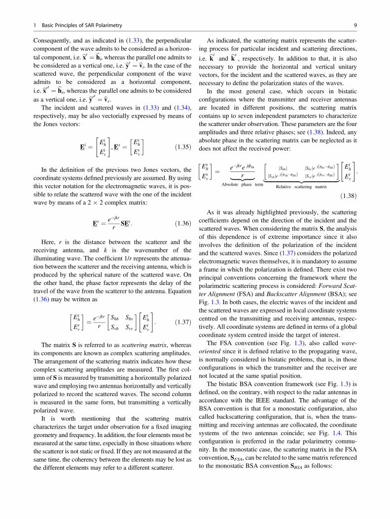
In the most general case, which occurs in bistaticconfigurations where the transmitter and receiver antennasare located in different positions, the scattering matrixcontains up to seven independent parameters to characterizethe scatterer under observation. These parameters are the fouramplitudes and three relative phases; see (1.38). Indeed, anyabsolute phase in the scattering matrix can be neglected as itdoes not affect the received power:

Esh

Esv

� �¼ e�jkre jϕhh

r|fflfflfflfflffl{zfflfflfflfflffl}Absolute phase term

Shhj j Shvj je j ϕhv�ϕhhð ÞSvhj je j ϕvh�ϕhhð Þ Svvj je j ϕvv�ϕhhð Þ

� �|fflfflfflfflfflfflfflfflfflfflfflfflfflfflfflfflfflfflfflfflfflfflfflffl{zfflfflfflfflfflfflfflfflfflfflfflfflfflfflfflfflfflfflfflfflfflfflfflffl}

Relative scattering matrix

Eih

Eiv

" #:

ð1:38Þ

As it was already highlighted previously, the scatteringcoefficients depend on the direction of the incident and thescattered waves. When considering the matrix S, the analysisof this dependence is of extreme importance since it alsoinvolves the definition of the polarization of the incidentand the scattered waves. Since (1.37) considers the polarizedelectromagnetic waves themselves, it is mandatory to assumea frame in which the polarization is defined. There exist twoprincipal conventions concerning the framework where thepolarimetric scattering process is considered: Forward Scat-ter Alignment (FSA) and Backscatter Alignment (BSA); seeFig. 1.3. In both cases, the electric waves of the incident andthe scattered waves are expressed in local coordinate systemscentred on the transmitting and receiving antennas, respec-tively. All coordinate systems are defined in terms of a globalcoordinate system centred inside the target of interest.

The FSA convention (see Fig. 1.3), also called wave-oriented since it is defined relative to the propagating wave,is normally considered in bistatic problems, that is, in thoseconfigurations in which the transmitter and the receiver arenot located at the same spatial position.

The bistatic BSA convention framework (see Fig. 1.3) isdefined, on the contrary, with respect to the radar antennas inaccordance with the IEEE standard. The advantage of theBSA convention is that for a monostatic configuration, alsocalled backscattering configuration, that is, when the trans-mitting and receiving antennas are collocated, the coordinatesystems of the two antennas coincide; see Fig. 1.4. Thisconfiguration is preferred in the radar polarimetry commu-nity. In the monostatic case, the scattering matrix in the FSAconvention, SFSA, can be related to the same matrix referencedto the monostatic BSA convention SBSA as follows:


SBSA ¼ �1 0

0 1

� �SFSA: ð1:39Þ

As it has been mentioned previously, in the radar polarim-etry community, the monostatic BSA convention (backscat-tering) is considered as the framework to characterize thescattering process. The reason to select this configuration isdue to the fact that the majority of the existing polarimetricradar systems operate with the same antenna for transmissionand reception. One important property of this configuration,for reciprocal targets, is reciprocity, which states that

ShvBSA ¼ SvhBSA , ð1:40Þ

ShvFSA ¼ �SvhFSA : ð1:41Þ

Then, the formalization of the scattering process given by(1.37), in the monostatic case under the BSA convention,reduces to

Esh

Esv

� �¼ e�jkr

rShh ShvShv Svv

� �Eih

Eiv

" #: ð1:42Þ

In the same sense, Eq. (1.38) takes the form

Esh

Esv

� �¼ e�jkre jϕhh

r|fflfflfflfflffl{zfflfflfflfflffl}Absolute phase term

Shhj j Shvj je j ϕhv�ϕhhð ÞShvj je j ϕhv�ϕhhð Þ Svvj je j ϕvv�ϕhhð Þ

� �|fflfflfflfflfflfflfflfflfflfflfflfflfflfflfflfflfflfflfflfflfflfflfflffl{zfflfflfflfflfflfflfflfflfflfflfflfflfflfflfflfflfflfflfflfflfflfflfflffl}

Relative scattering matrix

Eih

Eiv

" #:

ð1:43Þ

The main consequence of the previous equation is that inthe backscattering direction, a given scatterer is no longercharacterized by seven independent parameters, but by five.These are three amplitudes, two relative phases, and oneadditional absolute phase.

A central parameter when considering the scattering pro-cess occurring at a given scatterer consists of the scatteredpower. For single-polarization systems, the scattered power isdetermined by means of the radar cross section or the scatter-ing coefficient. Nevertheless, a polarimetric radar has to beconsidered as a multichannel system. Consequently, in orderto determine the scattered power, it is necessary to considerall the data channels, that is, all the elements of the scatteringmatrix. The total scattered power, in the case of a polarimetricradar system, is known as Span, being defined in the mostgeneral case as

SPAN Sð Þ ¼ trace SST��

¼ Shhj j2 þ Shvj j2 þ Shvj j2 þ Svvj j2: ð1:44Þ

In the backscattering case, due to the reciprocity theorem,the Span reduces to

SPAN Sð Þ ¼ Shhj j2 þ 2 Shvj j2 þ Svvj j2: ð1:45Þ

The main property of the Span is that it is polarimetricallyinvariable, that is, it does not depend on the polarization basisemployed to describe the polarization of the electromagneticwaves.

z

x

y

vi

hi

ki

vs

hs

ks

i s

s

i

^

^^

^

^

^

^

^

^

(a) (b)

z

x

y

vi

hi

ki

vs

hs

ks

i s

s

i

^

^^

^

^

^^

^

^

Fig. 1.3 (a) FSA and (b) BSA conventions


When the radar wave reaches a scatterer, part of theincident energy is reflected back to the system. If the incidentwave is monochromatic, the target is unchanging and theradar-target aspect angle is constant, the scattered wave willbe also monochromatic and completely polarized. Therefore,both the incident and the scattered waves can becharacterized by their corresponding Jones vectors, and thescattering process can be characterized by the scatteringmatrix. These targets are referred to as point targets, singletargets or deterministic targets, as when a radar images thistype of scatterers, the scattered wave in the far-field zoneappears to be originated by a single point. In other words, thetarget response is not contaminated by additional spurious, soit is possible to infer some information about the target fromthe single values of the scattering matrix. Table 1.6 shows thescattering matrix, expressed in the linear polarization basis,for some canonical bodies. These are referred to as canonicaldue to the simplicity of their scattering matrix.

1.1.2.2 Scattering Polarimetry DescriptorsThe scattering matrix introduced in the previous section isindeed a scattering polarimetry descriptor that could be alsoincluded in this section. Nevertheless, it merits a separatesection as this matrix represents the best vehicle to introducethe description of the scattering process when polarimetry isconcerned, as the scattering matrix relates the Jones vectorsof the involved electromagnetic waves. Section 1.1.1.1introduced additional descriptors for the polarization stateof an electromagnetic wave. As a consequence, some addi-tional descriptors for the scattering process shall beintroduced in the following.

The 2 � 2 complex scattering matrix, as indicated,describes the scattering matrix of a given target. Table 1.6presented several examples for some simple or canonicalscatterers. Nevertheless, a real target presents always a com-plex scattering response as a consequence of its complexgeometrical structure and its reflectivity properties. Conse-quently, the interpretation of this response is obscure. As itshall be presented later on, a possible solution to interpret this

response is to decompose the original scattering matrix intothe response of canonical mechanisms. With this idea inmind, but also with the objective to introduce a newformulism to extract physical information, it is possible totransform the scattering matrix into a scattering vector thatpresents a clearer physical interpretation.

The construction of a target vector k is performed throughthe vectorization of the scattering matrix:

k ¼ V Sð Þ ¼ 12trace SΨð Þ: ð1:46Þ

Ψ is a set of 2 � 2 complex basis matrices which areconstructed as an orthonormal set under a Hermitian innerproduct. The interpretation of the target vector k depends onthe selected basis Ψ. The most common matrix basesemployed in the context of the radar polarimetry are theso-called lexicographic ordering basis and the Pauli basis.The lexicographic ordering basis consists of the straightfor-ward lexicographic ordering of the elements of the scatteringmatrix:

Ψl ¼ 21 0

0 0

� �, 2

0 1

0 0

� �, 2

0 0

1 0

� �, 2

0 0

0 1

� �� :

ð1:47Þ

The Pauli basis consists of the set of Pauli spin matricesusually employed in quantum mechanics:

Ψp ¼ffiffiffi2

p 1 0

0 1

� �,ffiffiffi2

p 1 0

0 �1

� �,ffiffiffi2

p 0 1

1 0

� �,ffiffiffi2

p 0 �j

j 0

� �� :

ð1:48Þ

Note that the multiplying factor in both bases is necessaryin order to keep the total scattered power constant, i.e. trace(SS�T).

The selection of the basis to vectorize the scattering matrixdepends on the final purpose of the vectorization itself. When

a bFig. 1.4 (a) FSA and (b) BSAconventions in thebackscattering case


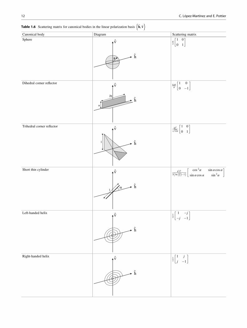
Table 1.6 Scattering matrix for canonical bodies in the linear polarization basis bh,bvn oCanonical body Diagram Scattering matrix

Spherea2

1 0

0 1

� �

Dihedral corner reflectorkabπ

1 0

0 �1

� �

Trihedral corner reflectorkl2ffiffiffiffi12

pπ

1 0

0 1

� �

Short thin cylinderk2 l3

3 ln 4lað Þ�1ð Þ

cos 2α sin α cos α

sin α cos α sin 2α

� �

Left-handed helix12

1 �j

�j �1

� �

Right-handed helix 12

1 j

j �1

� �


the objective is to study the statistical behaviour of the SARdata or the radar measurement, it is more convenient toconsider the lexicographic basis due to its simplicity, as itshall be extended in the next sections. Nevertheless, when theobjective is the physical interpretation of the scatteringmatrix, it is more convenient to consider the Pauli basis.Assuming the Pauli decomposition basis, an arbitrary 2 � 2scattering matrix may be written in the following terms:

S ¼ aþ b c� jd

cþ jd a� b

� �¼ a

1 0

0 1

� �þ b

1 0

0 �1

� �þ c

0 1

1 0

� �þ d

0 �j

j 0

� �: ð1:49Þ

It is worth noting that the elements a, b, c and d arecomplex. If one considers the decomposition of the scatteringmatrix as performed in (1.49), it is possible to identify thefour elements of the Pauli basis with some of the scatteringmatrices of canonical bodies presented in Table 1.6. There-fore, the elements a, b, c and d, i.e. the elements of the targetvector k, represent the contribution of every canonical mech-anism to the final scattering mechanism. Therefore, the fol-lowing interpretation is possible:

• a corresponds to the single scattering from a sphere orplane surface.

• b corresponds to dihedral scattering.• c corresponds to dihedral scattering with a relative orien-

tation of π/4 rad in the line of sight.• d corresponds to anti-symmetric, helix-type scattering

mechanisms that transform the incident wave into itsorthogonal circular polarization state (helix related).

All in all, what has been performed in (1.49) is a targetdecomposition. This concept shall be analysed in depth in thenext. It is also worth to notice that the different componentsof the Pauli basis, or scattering components, are orthogonal.This means that from a practical point of view, the separationindicated in (1.49) is possible without ambiguities.

Finally, the explicit expressions of the target vector in thelexicographic and Pauli decomposition bases, considering theexpression of the scattering matrix, in the most general caseare:

kl ¼

ShhShvSvhSvv

2666437775, kp ¼ 1ffiffiffi

2p

Shh þ SvvShh � SvvShv þ Svh

j Shv � Svhð Þ

2666437775 ð1:50Þ

In the backscattering case, under the BSA convention, thereciprocity property applies. Hence, the previous targetvectors admit the following simplification:

kl ¼Shhffiffiffi2

pShv

Svv

264375,kp ¼ 1ffiffiffi

2p

Shh þ Svv

Shh � Svv2Shv

264375 ð1:51Þ

The different 2 andffiffiffi2

pfactors that appear in the definition

of the target vectors are necessary in order to maintain thetotal scattered power or Span. As it is evident, the Span mustbe constant and independent from the choice of the basis inwhich the scattering matrix is decomposed. This is known astotal power invariance.

The concept of target vector, obtained as a vectorization ofthe scattering matrix, makes it possible to obtain a newformulation to describe the information contained in thescattering matrix by means of the outer product of the targetvector with its conjugate transpose, or adjoint vector.

For a vectorization of the scattering matrix through thelexicographic basis, in the most general case, the outer prod-uct of the target vector with its transpose conjugate klkT�lleads to the matrix:

klkT�l ¼

Shhj j2 ShhS�hv ShhS

�vh ShhS

�vv

ShvS�hh Shvj j2 ShvS�vh ShvS�vvSvhS

�hh SvhS

�hv Svhj j2 SvhS

�vv

SvvS�hh SvvS

�hv SvvS

�vh Svvj j2

266664377775: ð1:52Þ

Due to a language abuse, the matrix klkT�l is sometimesreferred to as covariance matrix and represented by C, but asit will be shown in Sect. 1.1.2.4, the covariance matrixpresents a different definition. It is worth to observe that(1.52) is a 4 � 4, complex, Hermitian matrix. The construc-tion of this matrix, through the outer product of the vector kland its transpose conjugate, makes the matrix klkT�l have arank equal to 1. Consequently, klkT�l presents exactly thesame information as the scattering matrix, and hence it mayhave up to seven independent parameters. In the case of thebackscattering direction under the BSA convention, and dueto the fact that the reciprocity relation applies, klkT�l can bewritten, considering (1.51), as

klkT�l ¼Shhj j2 ffiffiffi

2p

ShhS�hv ShhS

�vvffiffiffi

2p

ShvS�hh Shvj j2 ffiffiffi

2p

ShvS�vv

SvvS�hh

ffiffiffi2

pSvvS

�hv Svvj j2

264375: ð1:53Þ

As in the previous case, the klkT�l matrix presents a rankequal to 1 as it is obtained as the outer product of a vector and


its transpose conjugate. Nevertheless, in this case, the covari-ance matrix may present up to five independent parameters,that is, the same number of independent parameters as thescattering matrix from which it derives.

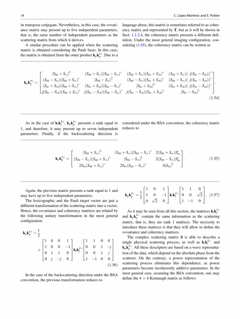
A similar procedure can be applied when the scatteringmatrix is obtained considering the Pauli basis. In this case,the matrix is obtained from the outer product kpkT�p . Due to a

language abuse, this matrix is sometimes referred to as coher-ency matrix and represented by T, but as it will be shown inSect. 1.1.2.4, the coherency matrix presents a different defi-nition. Under the most general imaging configuration, con-sidering (1.65), the coherency matrix can be written as

kpkT�p ¼Shh þ Svvj j2 Shh þ Svvð Þ Shh � Svvð Þ� Shh þ Svvð Þ Shv þ Svhð Þ� Shh þ Svvð Þ j Shv � Svhð Þð Þ�

Shh � Svvð Þ Shh þ Svvð Þ� Shh � Svvj j2 Shh � Svvð Þ Shv þ Svhð Þ� Shh � Svvð Þ j Shv � Svhð Þð Þ�Shv þ Svhð Þ Shh þ Svvð Þ� Shv þ Svhð Þ Shh � Svvð Þ� Shv þ Svhj j2 Shv þ Svhð Þ j Shv � Svhð Þð Þ�

j Shv � Svhð Þ Shh þ Svvð Þ� j Shv � Svhð Þ Shh � Svvð Þ� j Shv � Svhð Þ Shv þ Svhð Þ� Shv � Svhj j2

2666437775:

ð1:54Þ

As in the case of klkT�l , kpkT�p presents a rank equal to

1, and therefore, it may present up to seven independentparameters. Finally, if the backscattering direction is

considered under the BSA convention, the coherency matrixreduces to

kpkT�p ¼Shh þ Svvj j2 Shh þ Svvð Þ Shh � Svvð Þ� 2 Shh þ Svvð ÞS�hv

Shh � Svvð Þ Shh þ Svvð Þ� Shh � Svvj j2 2 Shh � Svvð ÞS�hv2Shv Shh þ Svvð Þ� 2Shv Shh � Svvð Þ� 4 Shvj j2

264375: ð1:55Þ

Again, the previous matrix presents a rank equal to 1 andmay have up to five independent parameters.

The lexicographic and the Pauli target vector are just adifferent transformation of the scattering matrix into a vector.Hence, the covariance and coherency matrices are related bythe following unitary transformation in the most generalconfiguration:

kpkT�p ¼ 12

�

1 0 0 1

1 0 0 �1

0 1 1 0

0 j �j 0

2666437775klkT�l

1 1 0 0

0 0 1 �j

0 0 1 j

1 �1 0 0

2666437775:

ð1:56Þ

In the case of the backscattering direction under the BSAconvention, the previous transformation reduces to

kpkT�p ¼ 12

1 0 1

1 0 �1

0ffiffiffi2

p0

264375klkT�l 1 1 0

0 0ffiffiffi2

p

1 �1 0

264375: ð1:57Þ

As it may be seen from all this section, the matrices klkT�land kpkT�p contain the same information as the scattering

matrix, that is, they are rank 1 matrices. The necessity tointroduce these matrices is that they will allow to define thecovariance and coherency matrices.

The complex scattering matrix S is able to describe asingle physical scattering process, as well as klkT�l andkpkT�p . All these descriptors are based on a wave representa-

tion of the data, which depend on the absolute phase from thescatterer. On the contrary, a power representation of thescattering process eliminates this dependence, as powerparameters become incoherently additive parameters. In themost general case, assuming the BSA convention, one maydefine the 4 � 4 Kennaugh matrix as follows:


K ¼ A� SO

S� �

A�1 ð1:58Þ

where

A ¼

1 0 0 1

1 0 0 �1

0 1 1 0

0 j �j 0

2666437775: ð1:59Þ

The Kennaugh matrix can be written in the followingform:

K ¼

A0 þ B0 Cψ Hψ Fψ

Cψ A0 þ Bψ Eψ Gψ

Hψ Eψ A0 � Bψ Dψ

Fψ Gψ Dψ �A0 þ B0

2666437775ð1:60Þ

where

A0 ¼ 14Shh þ Svvj j2

B0 ¼ 14Shh � Svvj j2 þ Shvj j2

Bψ ¼ 14Shh � Svvj j2 � Shvj j2

Cψ ¼ 12Shh � Svvj j2

Dψ ¼ ℑ ShhS�vv

Eψ ¼ ℜ S�hv Shh � Svvð Þ Fψ ¼ ℑ S�hv Shh � Svvð Þ Gψ ¼ ℜ S�hv Shh þ Svvð Þ Hψ ¼ ℑ S�hv Shh þ Svvð Þ

: ð1:61Þ

In the previous definition, the sub-index ψ indicates thatthe different parameters are roll angle dependent,corresponding to the target rotation along the line of sight.

As detailed in Sect. 1.1.2.1, the scattering matrix relatesthe scattered wave to the incident Jones vector. TheKennaugh matrix is related to the associated Stokes vectorsdefined in Sect. 1.1.1.1. In the forward scattering case, whereS is represented in the FSA coordinate formulation, thismatrix is named the 4� 4 Mueller matrix and is calculated by

M ¼ A SO

S� �

A�1: ð1:62Þ

The main difference ofK andM, with respect to klkT�l andkpkT�p , is that the Kennaugh and the Mueller matrices are real

matrices, whereas the covariance and coherency matrices arecomplex.

1.1.2.3 Partial Scattering PolarimetryAs indicated in Sect. 1.1.1.2, radar polarimetry is concernedwith two types of waves. The first type is monochromatic,totally polarized electromagnetic waves where the polariza-tion state is perfectly represented by the Jones vectors. Con-sequently, the scattering process can be completelyrepresented by any of the scattering polarimetry descriptorsdetailed in the previous section, and especially the scatteringmatrix. This situation appears when the radar transmits aperfectly monochromatic wave and this wave reaches anunchanging scatterer, resulting in a perfectly polarizedscattered wave. As mentioned, these targets are referred toas point targets or coherent targets. The most important pointto be considered when coherent scattering is addressed is todetermine the number of independent parameters necessaryto represent the scattering process. That is, to determine thenumber of independent parameters necessary to represent theoperator able to characterize the change of the polarizationstate of the scattered wave with respect to the incident wavethat occurs in the scattering process. In a monostatic configu-ration, the scattering operator describing the scattering,i.e. any of the matrix operators indicated in Sections 1.1.2.1and 1.1.2.2, may present up to five independent parameters.In the bistatic case, these descriptors may present up to sevenindependent parameters.

The situation changes when the scattering properties of thetarget being imaged by the radar system change in time, as itwould be the case for a forest being affected by the windconditions or, for instance, when the target presents morethan one scattering centre (a point at which the incident wavecan be considered to be reflected). Under this situation,although the radar system transmits a perfectly polarizedwave, the wave scattered by the scatterer is partiallypolarized. A scatterer of this category is normally referredto as distributed scatterer, depolarizing scatterer or an inco-herent scattering target. The change of the polarization stateof the scattered wave makes not possible to use the scatteringdescriptors presented in Sects. 1.1.2.1 and 1.1.2.2 to describethe scattering process, as these descriptors are not able todescribe the variation of the polarization state of thescattered wave.

In the case of partially polarized waves, the description ofthe polarization state must be addressed through polarizationdescriptors relying on the second-order moments of the elec-tromagnetic wave. If a wave is decomposed into two orthog-onal components in the plane perpendicular to thepropagation direction, these second-order moments refer tothe power of each orthogonal component and to the correla-tion between them. This information is perfectly representedby the vector and the wave coherency matrix or the Stokesvector. In the case of the description of the scattering process,this information can be perfectly represented by the covari-ance and coherency matrices as the mean values of thesematrices are not zero.


1.1.2.4 Change of Polarization BasisThe scattering properties of a given scatterer, asdemonstrated, are contained within the scattering matrix S,which, as shown previously, is measured in a particularpolarization basis. Since there exist an infinite number oforthonormal polarization bases, the question rising at thispoint is whether it is possible or not to infer the polarimetricproperties of the given target in any polarization basis fromthe response measured at a particular basis. This questionpresents an affirmative answer. The possibility to synthesizeany polarimetric response of a given target from its measure-ment in a particular orthonormal basis represents the mostimportant property of polarimetric systems in comparisonwith single-polarization systems. The most important conse-quence of this process is that the amount of information abouta given scatterer can be increased, allowing a better charac-terization and study. This polarization synthesis process isbased on the concept of change of polarization basispresented in Sect. 1.1.1.3.

Before describing the polarization synthesis process in thebackscattering direction, it is necessary to analyse the scatter-ing process given by (1.37) with respect to the direction ofpropagation of the incident and the scattered waves. It mustbe noticed that the incident wave propagates in the direction

given by the unitary vector bki , whereas the scattered one

propagates in the opposite direction, given by �bki . Conse-quently, this difference in the propagation direction must betaken into account when defining the polarization state of thewave. Given a Jones vector propagating in the direction bk, theJones vector of a wave presenting the same polarization statebut which propagates in the direction �bk is obtained as

bk ! �bk , E bk� � ¼ E� �bk� �ð1:63Þ

where, as mentioned previously, the BSA convention isconsidered. Under this assumption, the scattering matrix isreferred to as the coordinate system centred in the transmit-ting/receiving system. Consider a polarimetric radar systemwhich transmits the electromagnetic waves in the followingorthonormal basis bu, bu⊥f g. In this particular basis, the inci-dent and scattered waves are related by the scattering matrixas follows:

Es bu,bu⊥ ¼ S bu,bu⊥ Ei bu,bu⊥ : ð1:64Þ

As shown in Sect. 1.1.1.3, given the Jones vectormeasured in a particular basis, for instance, bu,bu⊥f g , it ispossible to derive it in any other polarization basis bu0,bu0⊥

,which may be rewritten as follows:

E bu0,bu0⊥ ¼ U bu,bu⊥ ! bu0 ,bu0⊥ E bu,bu⊥ : ð1:65Þ

Then, the incident and the scattered waves transformed inthe new basis may be considered:

Ei bu0 ,bu0⊥ ¼ U bu,bu⊥ ! bu0,bu0⊥ Ei bu,bu⊥ , ð1:66Þ

Es bu0,bu0⊥ ¼ U bu,bu⊥ ! bu0 ,bu0⊥ Es bu,bu⊥ : ð1:67Þ

In order to apply the transformation basis procedure to thescattered waves Es bu,bu⊥ , we need to consider that it

propagates in the opposite direction as the incident waveEi bu,bu⊥ . The transformation indicated by (1.64) assumes

that the incident and the scattered waves propagate in oppo-site directions, but (1.66) and (1.67) assume that both wavespropagate in the same direction. Consequently it is necessaryto consider the transformation indicated by (1.63) in (1.67).As a result, the transformation basis procedure applies to thescattered wave as follows:

Es bu0,bu0⊥ ¼ U�bu,bu⊥ ! bu0 ,bu0⊥ Es bu,bu⊥ ð1:68Þ

where now the wave in (1.68) is assumed to propagate inopposite direction with respect to the incident wave in (1.66).Now, it is possible to introduce (1.66) and (1.68) in (1.64):

U�bu0 ,bu0⊥ ! bu,bu⊥ Es bu0,bu0⊥ ¼S bu,bu⊥ U bu0,bu0⊥

! bu,bu⊥ Ei bu0 ,bu0⊥ :ð1:69Þ

As the transformation matrix U is unitary, i.e. U�1 ¼ U�T,

Es bu0 ,bu0⊥ ¼UTbu0,bu0⊥ ! bu,bu⊥ S bu,bu⊥ U bu0 ,bu0⊥

! bu,bu⊥ Ei bu0,bu0⊥ ð1:70Þ

from where it can be clearly identified the following identity

S bu0,bu0⊥ ¼ U�bu0 ,bu0⊥ ! bu,bu⊥ � ��1

S bu,bu⊥ U bu0,bu0⊥ ! bu,bu⊥ :

ð1:71Þ

The transformation expressed in (1.71) receives the nameof con-similarity transformation. This transformation allowsto synthesize the scattering matrix in an arbitrary basisbu0, bu0⊥

from its measure in the basis bu,bu⊥f g.

1.1.2.5 Scatterers Characterization by Single, Dual,Compact and Full Polarimetry

The main objective behind the use of polarimetric diversity,also known as full polarimetry, when observing a particularscatterer is that this type of diversity allows a far more


complete characterization of the scatterer than the characteri-zation that could be obtained without polarimetric sensitivity,or simply single-polarization measurements. Although thisimproved characterization, if compared with single-polarization data, the use of polarimetric diversity comes ata price, as the average transmitted power must be doubledand the swath width halved. In addition, a fully polarimetricSAR is technologically more complex than a single-polarization SAR system. In order to understand the differ-ence between these two philosophies and the improvement inthe characterization of a scatterer provided by polarimetry, itis necessary to introduce two important concepts, since theywill determine the way in which a target shall becharacterized. It may happen the scatterer of interest to besmaller than the coverage of the radar system. In this situa-tion, we consider the scatterer as an isolated scatterer, andfrom a point of view of power exchange, this target ischaracterized by the so-called radar cross section. Neverthe-less, we can find situations in which the scatterer of interest issignificantly larger than the coverage provided by the radarsystem. In these occasions, it is more convenient to charac-terize the target independently of its extent. Hence, in thesesituations, the target is described by the so-called scatteringcoefficient.

The most fundamental form to describe the interaction ofan electromagnetic wave with a given scatterer is theso-called radar equation. This equation establishes the rela-tion between the power the scatterer intercepts from theincident electromagnetic wave and the power reradiated bythe same scatterer in the form of the scattered wave. The radarequation presents the following form:

Pr ¼ PtGt

4πr2tσ

Ar

4πr2rð1:72Þ

where Pr represents the power detected at the receivingsystem. The term

PtGt

4πr2tð1:73Þ

is determined by the incident wave, and it consists of itspower density expressed in terms of the properties of thetransmitting system. The different terms in (1.73) are thetransmitted power Pt, the antenna gain Gt and the distancebetween the system and the target rt. On the contrary, theterm

Ar

4πr2rð1:74Þ

contains the parameters concerning the receiving system: theeffective aperture of the receiving antenna Ar and the distancebetween the target and the receiving system rr. The last termin (1.72), i.e. σ, determines the effects of the scatterer ofinterest on the balance of powers established by the radarequation. Since (1.73) is a power density, i.e. power per unitarea, and (1.74) is dimensionless, the parameter σ has units ofarea. Consequently, σ consists of an effective area whichcharacterizes the scatterer. This parameter determines whichamount of power is intercepted from (1.73) by the scattererand reradiated. This reradiated power is finally intercepted bythe receiving system according to the distance rt. An impor-tant fact which arises at this point is the way the scattererreradiates the intercepted power in a given direction of thespace. In order to be independent of this property, the radarcross section shall be referenced to an idealized isotropicscatterer. Thus, the radar cross section of an object is thecross section of an equivalent isotropic scatterer thatgenerates the same scattered power density as the object inthe observed direction:

σ ¼ 4πr2E!s�� 2E!i�� 2

¼ 4π Sj j2 ð1:75Þ

where E!�� 2 represents the intensity of the electromagnetic

wave and S is the complex scattering amplitude of the object.The final value of σ is a function of a large number ofparameters which are difficult to consider individually: thewave frequency, the wave polarization, the imaging geome-try or the geometrical structure and the dielectric properties ofthe scatterer. Then, the radar cross section σ is able to char-acterize the target being imaged for a particular frequencyand imaging system configuration.

The radar equation, as given by (1.72), is valid for thosecases in which the scatterer of interest is smaller than theradar coverage, that is, a point target or point scatterer. Forthose targets presenting an extent larger than the radar cover-age, we need a different model to represent the scatterer. Inthese situations, a scatterer is represented as an infinite col-lection of statistically identical point scatterers. The resulting

scattered wave E!s

results from the coherent addition of thescattered waves from every one of the independent scattererswhich model the extended scatterer. In order to express thescattering properties of the extended target independently ofits area extent, we consider every elementary target as beingdescribed by a differential radar cross section dσ. In order toseparate the effects of the target extent, we consider dσ as theproduct of the averaged radar cross section per unit area


σ0 and the differential area occupied by the target ds. Then,the differential power received by the systems due to anelementary scatterer can be written as

dPr ¼ PtGt

4πr2tσ0ds

Ar

4πr2r: ð1:76Þ

Hence, to find the total power received from the extendedtarget, we need to integrate over the illuminated area A0:

Pr ¼ZZA0

PtGt

4πr2tσ0

Ar

4πr2rds: ð1:77Þ

It must be noted that the radar equation at (1.72) representsa deterministic problem, whereas (1.77) considers a statisticalproblem. Eq. (1.77) represents the average power returnedfrom the extended target. Hence, the radar cross section perunit area σ0, or simply scattering coefficient, is the ratio of thestatistically averaged scattered power density to the averageincident power density over the surface of the sphere ofradius rr:

σ0 ¼ E σf gA0

¼ 4πr2rA0

E E!s�� 2� �E!i�� 2

: ð1:78Þ

The scattering coefficient σ0 is a dimensionless parameter.As in the case of the radar cross section, the scatteringcoefficient is employed to characterize the scattered beingimaged by the radar. This characterization is for a particularfrequency f, polarization of the incident and scattered wavesand incident and scattering directions.

As it has been shown, the characterization of a givenscatterer by means of the radar cross section σ or the scatter-ing coefficient σ0 depends also on the polarization of the

incident wave E!i

. As one can observe in (1.75) and (1.78),these two coefficients are expressed as a function of theintensity of the incident and scattered waves. Consequently,σ and σ0 shall be only sensitive to the polarization of theincident waves through the effects the polarization has overthe power of the related electromagnetic waves. Hence, if wedenote by p the polarization of the incident wave and by q thepolarization of the scattered wave, we can define the follow-ing polarization-dependent radar cross section and scatteringcoefficient, respectively:

σqp ¼ 4πr2E!s

qp

�� 2E!i

qp

�� 2¼ 4π Sqp

�� 2, ð1:79Þ

σ0qp ¼E σqp A0

¼ 4πr2rA0

E E!s

qp

�� 2� �E!i

qp

�� 2: ð1:80Þ

As it has been shown, a given target of interest can becharacterized by means of the radar cross section or thescattering coefficient depending on the nature of the scattereritself; see (1.75) and (1.78). Additionally, in (1.79) and(1.80), it has been shown that these two coefficients dependalso on the polarization of the incident and the scatteredelectromagnetic waves. A closer look to these expressionsreveals that these two real coefficients depend on the polari-zation of the electromagnetic waves only through the powerassociated with them. Thus, they do not exploit, explicitly,the vectorial nature of polarized electromagnetic waves. ASAR system that measures σ or σ0 is usually referred to assingle-polarization SAR systems as, normally, the samepolarization is employed for transmission and for reception.In this case, the products delivered by the SAR system arereal SAR images containing the information of σ or σ0.

In order to take advantage of the polarization of the elec-tromagnetic waves, that is, their vectorial nature, the scatter-ing process at the scatterer of interest must be considered as afunction of the electromagnetic waves themselves. In Sect.1.1.1.1, it was shown that the polarization of a plane, mono-chromatic, electric wave could be represented by theso-called Jones vector. Additionally, a set of two orthogonalJones vectors form a polarization basis, in which any polari-zation state of a given electromagnetic wave can beexpressed. Therefore, given the Jones vectors of the incidentand the scattered waves, Ei and Es, respectively, the scatter-ing process occurring at the target of interest is represented bythe scattering matrix S. In contraposition to a single-polari-zation SAR system, a fully polarimetric SAR systemmeasures the complete scattering matrix S. Therefore, theproduct delivered by this type of SAR systems correspondsto the 2� 2 complex scattering matrix and not individual realSAR images.

As it can be observed, the polarimetric sensitivity of ameasurement ranges from a complete absence of polarimetricsensitivity in the case of single-polarization SAR systems toa complete sensitivity in the case of fully polarimetric SARsystems. Polarimetric sensitivity comes to a price of a morecomplex system that implies, on the one hand, a heaviersystem and, on the other hand, the need to transmit a largerpower. In addition, and due to the need to double the pulserepetition frequency to accommodate two polarizations intransmission, the radar swath is also reduced. Nevertheless,between both architectures, there exist other polarimetricradar configurations with may soften the previous limitationsbut at the cost of reducing the amount of acquiredinformation.


A single-polarization or mono-polarization SAR systemis composed of one transmission and one reception chain thatoperate at a fixed polarization. In most of the cases, bothchains operate at the same polarization providing a co-pol orco-polarized channel. In the particular case of the linearpolarization basis, these channels would correspond to σhhor σ0hh and σvv or σ0vv for the horizontal and the verticalpolarization states, respectively. As indicated, these simpleimaging radars deliver real SAR images, proportional to σ orσ0, as products. One possibility to increase the amount ofinformation is to consider a dual-polarized radar by includinga second reception chain in the system, in such a way that ittransmits in one polarization, for instance, h, and it receivessimultaneously on the same polarization h and also on theorthogonal one v, leading to one co-pol and the so-calledco-polarized and the cross-polarized channels, respectively.A different alternative for a dual-polarized system is toconsider a transmission chain that alternates betweenpolarizations and a single reception chain. In all these cases,the polarimetric system provides images proportional to theradar brightness.

All the previous SAR systems present the limitation thatthe information that may be retrieved is restricted to the

information that can be extracted from the real SAR images,proportional to σ or σ0, or their different combinations. Nev-ertheless, this limitation is overcome by allowing two simul-taneous and coherent reception channels operating atorthogonal polarizations, making it possible to measure therelative phase between them. The coherent nature of thereceiving channels allows measuring the different elementsof the covariance or coherency matrix. The first option thatmay be considered is to assume a fixed polarization in trans-mission and orthogonal polarizations in reception. In the caseof the transmission channel, the circular polarization and the45� linear polarizations have been proposed, whereas forreception the horizontal and vertical linear polarizations areassumed. This type of systems are collectively known ascompact polarized systems as, although they allow to mea-sure some of the elements of the covariance and coherencymatrix, they do not allow to measure the complete matrices.Finally, by allowing the system to transmit alternativelybetween orthogonal polarizations and to receive coherentlyat the same two orthogonal polarizations, a system like this isable to measure coherently the scattering matrix and to pro-duce the covariance and coherency matrices. In the case of abistatic configuration, without any type of assumption, these

Fig. 1.5 The family of polarization diversity and polarimetric imaging radars. (Courtesy of Dr. R. K. Raney)


will be 4 � 4 complex matrices, whereas in the case of amonostatic configuration, these will be 3 � 3 complex matri-ces. Figure 1.5 details the complete hierarchy of polarimetricSAR systems.

1.2 SAR Data Statistical Descriptionand Speckle Noise Filtering

Most of geophysical media, for instance, rough surfaces,vegetation, ice, snow, etc., have a very complex structureand composition. Consequently, the knowledge of the exactscattered electromagnetic wave, when illuminated by an inci-dent wave, is only possible if a complete description of thescene was available. This type of description of the scatterersis unattainable for practical applications. The alternative,hence, is to describe them in a statistical form. Such scattersare named, consequently, as distributed or partial scatterers(Ulaby et al. 1986a, b).

SAR systems are mainly employed for natural scenesobservation. Owing to the complexity of these scatterers,the scattered wave has also a complex behaviour. Hence,the scattering process itself needs to be analysed stochasti-cally. Most of the techniques focused on solving the scatteredwave problem trying to find, hence, the statistical moments ofthe scattered wave as a function of the incident waveproperties, as well as the scatterer features.

In order to derive a stochastic model for the observed SARimages in the case of distributed scatterers, it is necessary toconsider a model for the SAR imaging process, a model forthe scattering process and a model for the distributed scatterbeing imaged.

The SAR imaging process is divided into two main pro-cesses. The former consists of the acquisition of the scattereddata, as a result of the illuminating wave, whereas the lattercomprises the focusing process. The second, which is incharge of collecting all the contributions of a particularscatterer focusing it as good as possible, tries to remove theeffects of the acquisition process. The SAR impulseresponse, or SAR system model, embracing the acquisition,as well as the focusing processes, can be assumed to be arectangular low-pass filter (Curlander and McDonough1991):

h x, rð Þ / sincπxδx

� �sinc

πrδr

� �: ð1:81Þ

In the previous equation, x and r indicate the azimuth andslant-range (simply called range in the following)dimensions of the SAR image, respectively, whereas δx andδr indicate the spatial resolutions in the same spatialdimensions. Finally, a SAR image, i.e. S(x, r), may be

modelled as a two-dimensional low-pass filter, given by(1.81), applied to the scene’s complex reflectivity σs(x, r)(Curlander and McDonough 1991):

S x, rð Þ ¼Z1�1

Z1�1

σs x0, r0ð Þh x� x0, r � r0ð Þdx0dr0: ð1:82Þ

Since the spatial resolutions of the SAR impulse response,δx and δr, are not zero, it is possible to introduce the conceptof resolution cell as the area given by δx � δr . Qualitatively,in the absence of signal re-sampling, the informationcontained by an image pixel is basically determined by theaverage complex reflectivity σs(x, r) within thisresolution cell.

The resolution cell dimensions, δx and δr, are larger thanthe wavelength of the illuminating electromagnetic wave λ.As a consequence, the resulting scattered wave is due to anelaborated scattering process. In order to arrive to a tractablemathematical model of the SAR image S(x, r), it is conve-nient to find an approximation for the scattering processwithin the resolution cell. The most common simplificationis the Born approximation or simple scattering approximation(Ulaby et al. 1986a). Under it, first, the distributed scatterer isconsidered to be composed of a set of discrete scattererscharacterized by a deterministic response. This scatterermodel might be reasonable for those cases in which thediscrete scatterer description is valid, for instance, scatteringfrom raindrops or vegetation-covered surfaces having leavessmall compared with the wavelength. On the contrary, thisassumption is not valid for continuous scatterers. In thesecases, it is helpful to apply the concept of effective scatteringcentre (Ulaby et al. 1986a), in which the continuous scattereris analysed in a discrete way, e.g. the facet model for surfacescattering (Ulaby et al. 1986a; Beckmann and Spizzichino1987). In a second step, the scattered wave from the resolu-tion cell is supposed to be the linear coherent combination ofthe individual scattered waves of each one of the discretescatters within the cell. The main limitation of the Bornapproximation is that it excludes attenuation or multiplescattering in the process.

Assuming the scattered wave from any distributedscatterer to be originated by a set of discrete sources, (1.82)can be considered in its discrete form:

S x, rð Þ ¼XNk¼1

σs xk , rkð Þh x� xk , r � rkð Þ ð1:83Þ

where the sub-index k refers to each particular discretescatterer in the resolution cell and N is the total number ofthese scatterers embraced by the response of the SAR systemh(x, r). Equation (1.83) can be rewritten by using


σs xk, rkð Þ ¼ ffiffiffiffiffiσk

pexp jθ0sk

� �, ð1:84Þ

h x� xk, r � rkð Þ ¼ hk exp jφkð Þ, ð1:85Þ

θsk ¼ θ0sk þ φk, ð1:86Þ

as follows:

S x, rð Þ ¼XNk¼1

Ak exp jθskð Þ ð1:87Þ

where Ak ¼ hkffiffiffiffiffiσk

p. As observed in (1.87), the process to

form a SAR image pixel consists of the complex coherentaddition of the responses of each one of the discretescatterers, which are not accessible individually. The soleavailable measure is the complex coherent addition itself.This coherent addition process receives the name ofbi-dimensional random walk (McCrea and Whipple 1940;Doob et al. 1954).

At this point, it is necessary to consider certainassumptions about the elementary scattered wavesAk exp jθskð Þ in order to derive a stochastic model for theobserved SAR image (Beckmann and Spizzichino 1987;Goodman 1985):

• The amplitude Ak and the phase θsk of the k-th scatteredwave are statistically independent of each other and fromthe amplitudes and phases of all other elementary waves.This fact states that the discrete scatterers are uncorrelatedand that the strength of a given scattered wave bears norelation to its phase.

• The phases of the elementary contributions θsk are equallylikely to lie anywhere in the primary interval [�π, π).

Under these conditions, (1.87) may be seen as an interfer-ence process, in which the interference itself is determined bythe phases θsk . This interference can be constructive, as wellas destructive. This effect can be clearly noticed in SARimages, as the amplitude or the intensity of (1.87) presentsa salt and pepper or grainy aspect, as it may be observed inFig. 1.6, which corresponds to |Shh| acquired with theRADARSAT-2 system over the city of San Francisco. Sucha phenomenon is known as speckle (Goodman 1985; Lee1981; Lopes et al. 1990; Raney 1983).

Speckle is a true electromagnetic measurement and has acomplete deterministic nature, as shown in (1.87). Neverthe-less, the information contained within speckle needs fromtwo different analyses. In those cases in which there is areduced number of discrete scatterers within the resolutioncell, or its response is basically originated by a reduced set of

Fig. 1.6 RADARSAT-2 amplitude image of the scattering matrix element Shh over San Francisco (USA)


dominant ones, speckle is said to be partially developed.Hence, the interference itself, i.e. the speckle, contains infor-mation about the scattering process. On the contrary, whenthere is a large number of discrete scatterers in the cell,without a dominant one, the interference process becomesso complex that it does contain almost no information aboutthe scattering process itself (Oliver and Quegan 1998). Thiscase is called fully developed speckle (Ulaby et al. 1986a),and the complexity of the interference process is overcomeby analysing it by statistical means. Hence, speckle turns tobe considered as a noise-like signal (Ulaby et al. 1986b;Lopes et al. 1990).

Summarizing, due to the lack of knowledge about thedetailed structure of the distributed scatterer being imagedby the SAR system, it is necessary to discuss the properties ofthe scattered wave statistically. The statistics of concern aredefined over an ensemble of objects, all with the same mac-roscopic properties, but differing in the internal structure. Fora given SAR system imaging a particular scatterer, e.g. arough surface, the exact value of each pixel cannot bepredicted, but only the parameters of the distribution describ-ing the pixel values. Therefore, for a SAR image, the actualinformation per pixel is very low as individual pixels arerandom samples from distributions characterized by areduced set of parameters.

1.2.1 One-Dimensional Gaussian Distribution

Considering a SAR system to be described by a rectangularlow-pass filter (see (1.81)) and the distributed scatterer to bemodelled by a set of discrete deterministic scatterers, bymeans of the single or Born scattering approximation, aSAR image, S(x, r), can be described by the model presentedin (1.87).

The main parameter in the SAR image model is thenumber of discrete scatterers within the resolution cell,i.e. N. Depending on the nature of this parameter, differentSAR image statistical models can be derived. On the onehand, if N is considered as a constant value, provided that it islarge enough, (1.87) leads to the complex, zero-mean, com-plex Gaussian pdf model, valid for homogeneous,non-textured SAR images (Beckmann and Spizzichino1987; Goodman 1985; Papoulis 1984). On the other hand,to consider N as a random variable makes (1.87) to lead to pdfmodels valid for textured areas description. In the following,the zero-mean, complex Gaussian distribution model shall beconsidered, although possible extensions to textured imagemodels shall be indicated.

When the number of discrete scatterers inside the resolu-tion cell N is large, provided that Ak cos ( jθk) and Ak sin ( jθk)satisfy the central limit theorem (Oliver and Quegan 1998),

the quantities ℜ{S} and ℑ{S} are Gaussian distributed, thatis, they follow a zero-mean, Gaussian probability densityfunction (pdf). The parameters of this pdf can be obtainedon the basis of the discrete scatterers model. The mean valuesof ℜ{S} and ℑ{S} are equal to zero, and the variances areE ℜ2 Sf g ¼ E ℑ 2 Sf g ¼ N

2 E Ak2

. Besides, the symme-

try of the phase distribution of the discrete scatterers produces(Beckmann and Spizzichino 1987):

E ℜ Sf gℑ Sf gf g ¼XNk¼1

�XNl¼1

E AkAlf gE cos θkð Þ sin θlð Þf g

¼ 0:

ð1:88Þ

Under these conditions, ℜ{S} and ℑ{S}, denoted in thefollowing by x and y, respectively, are described by means ofzero-mean Gaussian pdfs:

px xð Þ ¼ 1ffiffiffiffiffiffiffiffiπσ2

p exp � xσ

� �2� �, x 2 �1,1ð Þ ð1:89Þ

py yð Þ ¼ 1ffiffiffiffiffiffiffiffiπσ2

p exp � yσ

� �2� �, y 2 �1,1ð Þ ð1:90Þ

where the variance is σ2 ¼ (N/2)E{Ak2}. The pdfs px(x) and

py(y) are denoted in the following as N 0, σ2ð Þ. Consequently,a SAR image, S¼ x + jy¼ A exp ( jθ), is described by a zero-mean, complex, Gaussian distribution, with uncorrelated realand imaginary parts, denoted next as N 0, σ2ð Þ. From (1.89)and (1.90), it is straightforward to derive pA(A) and pθ(θ),where A ¼

ffiffiffiffiffiffiffiffiffiffiffiffiffiffix2 þ y2

pand θ ¼ arctan (y/x), as:

pA,θ A, θð Þ ¼ Aπσ2

exp � Aσ

� �2� �ð1:91Þ

pA Að Þ ¼ 2Aσ2

exp � Aσ

� �2� �, A 2 0,1½ Þ ð1:92Þ

pθ θð Þ ¼ 12π

, θ 2 �π, π½ Þ: ð1:93Þ

The amplitude pdf, i.e. pA(A), is known as Rayleigh distri-bution. In addition, if intensity, i.e. I ¼ A2, is considered, theRayleigh pdf is transformed to an exponential pdf:

pI Ið Þ ¼ 1σ2

exp � Iσ2

� �, I 2 0,1½ Þ: ð1:94Þ


On the other hand, (1.93) shows that the SAR image phasehas a uniform pdf. Consequently, this phase bears no infor-mation concerning the natural scene being imaged.

Given the SAR image amplitude pdf (1.92), the amplitudemean value is equal to σ

ffiffiffiπ

p=2, whereas the variance equals

(1 � (π/4))σ2. If the coefficient of variation, defined as thestandard deviation divided by the mean, is calculated, itequals

ffiffiffiffiffiffiffiffiffiffiffiffiffiffiffiffiffiffiffiffi4=πð Þ � 1

p. For the intensity I, it has a value equal

to 1 as the mean and the variance are equal to σ2. As aconsequence, the intensity of a SAR image can be modelledas the product of two uncorrelated terms (Goodman 1985;Lee 1981; Lopes et al. 1990; Raney 1983), i.e.

I ¼ σ0n: ð1:95Þ

The deterministic-like value is given by its mean, i.e. σ0,which corresponds to the mean incoherent power of the areaunder study (1.78). The random process n, with mean andvariance equal to 1, is characterized by an exponential pdfand is defined as the speckle noise component. As it may beobserved from the model (1.94) and (1.95), if the mean valueof the intensity increases, the variance increases as well.Therefore, this model is known as the multiplicative specklenoise model. In other words, the signal to noise ratio of theimage cannot be improved by increasing the transmittedpower, as the variance of the data will increaseproportionally.

The Gaussian model for SAR data, leading to (1.91) and(1.95), is able to characterize SAR data for homogeneousareas. In this case, useful information is described by a singledegree of freedom, corresponding to the mean intensity.Nevertheless, for certain types of distributed scatterers, sucha simple model cannot describe all the data variability. Thereason behind this limitation is that this type of scatterersneed from a more sophisticated model, with more than onedegree of freedom, in order to be completely described.Collectively, these models are able to describe average inten-sity variations, which correspond to data texture (Oliver andQuegan 1998). A variety of two-degree of freedom pdfmodels have been proposed in the literature, for instance:K-distribution (Kong 1990), Weibull distribution orlog-normal distribution (Oliver and Quegan 1998; Papoulis1984; Kong 1990). All these models consist of assuming thenumber of scatterers N, within a resolution cell, no longer as aconstant, but being described also by a certain distribution.Even so, there are situations in which these two-parametermodels are not able to describe the scene. Hence, the solutiongoes into the direction of introducing more degrees of free-dom, thus resulting in more elaborate image models (Oliverand Quegan 1998; Trunk and George 1970; Trunk 1972;Schleher 1975).

1.2.2 Multidimensional Gaussian Distribution

The previous section was concerned with the statisticaldescription of one-dimensional complex data acquired by acomplex SAR system, i.e. a single SAR image. As shown,despite the data’s complex nature, only the amplitude, or theintensity, contains useful information concerning thedistributed target under analysis. The amount of informationcan be increased by acquiring more than one SAR image, ifone or more imaging parameters, e.g. system position, acqui-sition time, frequency or polarization, are varied. What it ispursued, hence, is the study of the variation of the scatterer’sresponse to changes of the SAR system parameters. Thevolume of information is increased as more data channelsare available but also because, if available, the multidimen-sional data correlation structure can be also exploited toextract information about the observed scatterer (Oliver andQuegan 1998; Cloude and Pottier 1996). The following listshows the most common multidimensional SARconfigurations, as well as their main applications:

• SAR Interferometry (InSAR) (Bamler and Hartl 1998): Inthis configuration, two SAR systems image the samescene from slightly different positions in space, leadingto two-dimensional SAR data. In this way, the phasedifference between the two acquisitions is proportionalto the terrain’s topography. This configuration is exten-sively employed nowadays to obtain Digital ElevationModels (DEMs) of the terrain.

• Differential SAR Interferometry (DInSAR) (Gabriel et al.1989): This SAR configuration admits several variants.On the one hand, a differential interferogram can beobtained through the difference of two interferogramsacquired with a zero spatial baseline, but at differenttimes. Consequently, the “residual” differential interfero-gram can contain small topographic deformations or evenatmospheric effects. On the other hand, the same effectcan be observed if the topography of a given interferogramis compensated for by means of an external DEM.

• SAR Polarimetry (PolSAR) (Ulaby and Elachi 1990): Inthis case, the parameters which vary between the differentinformation channels are the polarization of the transmit-ted wave and the polarization with which the scatteredwave by the terrain is collected. A set of two orthogonalpolarization states are employed, being the most commonthe pair of horizontal and vertical polarizations. The mostimportant property of polarimetry is that the polarimetricresponse to any polarization state of the incident wave of agiven scatterer can be derived from the response to a pairof orthogonal polarization states. This SAR configurationexploits the fact that scatterers present different responses


to different polarizations of the incident wave. For back-scattering in which waves are transmitted and collected inthe same position and by considering the reciprocity theo-rem, PolSAR leads to three-dimensional data. On thecontrary, when scattered waves are collected in a differentposition with respect to the transmitted one, i.e. forwardscattering, PolSAR data are four-dimensional data.

• Polarimetric SAR Interferometry (PolInSAR) (Cloude andPapathanassiou 1998): This technique tries to combine boththe advantages of InSAR and PolSAR. On the one hand,the introduction of interferometric diversity makes possiblethe data to be sensible to the structure of the target in thevertical dimension. On the other hand, the data are relatedto different scattering mechanisms in the same resolutioncell, thanks to the polarimetric capabilities of the acquisi-tion system. Hence, PolInSAR data are sensible to differentscattering mechanisms in the same image pixel, located atdifferent heights. The introduction of simple scatteringmodels allows to extract relevant information about thescatterer under study. Among the possible applications ofthis technique, the most important is the extraction ofparameters related to the vegetation cover which allowbiomass estimation. In terms of data dimensionality,PolInSAR data consist of six-dimensional data if backscat-tering is considered, whereas they are eight-dimensionaldata for forward scattering.

• SAR Tomography (TomoSAR) (Reigber and Moreira2000): As shown in the previous point, PolInSARrepresents a first step to resolve the vertical structure ofthe imaged scatterer. In this direction, SAR tomography isa technique directed to achieve a real three-dimensionalreconstruction of the scene under observation. Both theSAR data acquisition and processing are based on thegeneration and processing of a synthetic aperture in theazimuth direction to reconstruct the object in this direc-tion. In the same way, SAR tomography is based on thesynthesis of an aperture in the dimension perpendicular tothe plane formed by the azimuth and range dimensions, byacquiring several SAR images in the vertical dimension.Consequently, the phase information of these images canbe employed to reconstruct, with enough spatial resolu-tion, the vertical structure of the scatterer.

• Multifrequency SAR (Sarabandi 1997; Lee et al. 1991): Asshown in the literature, the response of a given scattererdepends on frequency. Consequently, in order to extractthe maximum amount of information concerning thescatterer, several SAR images can be acquired at differentfrequencies. Therefore, the dimensionality of the datadepends on the number of acquired images.

From a general point of view, a multidimensional SARsystem acquires a set of SAR images, represented by thecomplex vector

k ¼ S1, S2, . . . , Sm½ �T ð1:96Þ

where m represents the number of SAR images, i.e. the datadimensionality, according to the previous description. Eachelement of the vector k, i.e. Si for i¼ 1, 2, . . ., m, represents asingle complex SAR image. In PolSAR, the k vector receivesthe name of scattering or target vector (in the straightforwardlexicographic basis), and it represents a vectorization of thescattering matrix S as detailed in Sect. 1.1.2.2. The correla-tion structure of the vector k, provided that its m componentsSi N 0, σ2ð Þ, is completely characterized by the Hermitiancovariance matrix C, defined as follows:

C ¼ E kkH

¼

E S1SH1

E S1S

H2

⋯ E S1S

Hm

E S2S

H1

E S2S

H2

⋯ E S2S

Hm

⋮ ⋮ ⋱ ⋮

E SmSH1

E SmS

H2

⋯ E SmS

Hm

26664

37775: ð1:97Þ

In the particular case of PolSAR data, the data correlationstructure can be also expressed by the Hermitian coherencymatrix Τ (Cloude and Pottier 1996). Considering (1.97), onecan see that the complex vector k is characterized by thefollowing pdf (Lee et al. 1994; Tough et al. 1995):

pk kð Þ ¼ 1πm Cj j exp �kHC�1k

� �: ð1:98Þ

Hence, (1.98) represents the data pdf model for a set ofm correlated SAR images, which is denoted in the followingas N 0,Cð Þ. Since k ~N 0,Cð Þ, it is completely characterizedby the first and the second central moments, i.e. the meantarget vector and the covariance matrix, respectively.

At this point, it is important to consider, as presentedbefore, the issue that the mean value of the real and imaginaryparts of k equals zero. The main consequence is that itprevents the possibility to extract useful information via anestimation of this mean value. For instance, this circumstancedetermines the way PolSAR data has to be considered whendistributed scatterers are of concern. A PolSAR systemmeasures the 2 � 2 complex scattering matrix S, which canbe vectorized into the form presented by (1.96) (Cloude andPottier 1996; Bebbington 1992); see also Sect. 1.1.2.2. Onthe one hand, when this scattering vector refers to adistributed scatterer, a given sample of it has almost noinformation concerning the scatterer itself, as k consists of asample of the pdf given by (1.98) (Oliver and Quegan 1998).On the other hand, if the mean value of k is estimated, it turnsout to be zero. Thus, as reported in the literature, whendistributed scatterers are studied, the vector k, or the scatter-ing matrix S in the particular case of PolSAR, cannotcompletely describe the properties of the distributed scatterer.


Therefore, it is necessary to characterize these properties bymeans of higher-order moments, i.e. through an estimation ofthe covariance matrix C, or, additionally, the coherencymatrix Τ. These two matrices are derived through the outerproduct of the target vectors kl and kp, respectively, asindicated in Sect. 1.1.2.2, so they are independent of theabsolute phase of the scattering matrix S or the target vectorskl and kp. Hence, the expected value in (1.97) needs to beestimated. The process to estimate the covariance matrix C isalso referred to as the polarimetric speckle noise removalprocess, as the objective is to remove the variability of thedata making it possible to retrieve the C matrix.

In the rest, the complex, multidimensional Gaussianmodel, presented by (1.98), is taken as the multidimensionalSAR imagery model. As for the one-dimensional model for asingle SAR image, the complex, multidimensional Gaussianmodel can be considered valid for homogeneous areas, thatis, areas in which the statistical properties of the data remainconstant. The main reason of this choice has to be found inthe fact that the simplicity of the complex, multidimensionalGaussian pdf, makes it possible the analytical analysis of theinformation which can be extracted from the data. In addi-tion, many studies reported in the literature support thismodel.

The multidimensional, zero-mean, complex Gaussian pdfmodel is based on the following assumptions:

• The distributed scatterer may be modelled as a collectionof discrete or point scatterers, whereas the scattering pro-cess occurring at the surface, or within it, is consideredunder the Born or simple scattering approximation.

• The properties of the distributed scatterer remain constantin space, hence leading to homogeneous SAR data.

Thus, whenever any of the previous two suppositions arenot fulfilled, SAR data can no longer be assumed to bedescribed by the complex, multidimensional Gaussian pdfmodel. These departures have been noticed in the literatureat high resolutions or high frequencies, giving rise to datatexture. As for one-dimensional SAR imagery, some of thesedepartures can be explained by considering N, the total num-ber of scatterers in the resolution cell, to be described by acertain pdf. If the mean number of scatterers contributing tothe measurement at each pixel is large, then whatever the pdfof the number of discrete scatterers, the vector k can berepresented by the product of two independent processes:

k ¼ Tk0, ð1:99Þ

where T is a positive scalar texture and k0 is a complex,multidimensional Gaussian distributed vector, with the

same covariance as k. When T is considered to be describedby a square-root gamma pdf, the data k in (1.99) is describedby the so-called K-distribution (Kong 1990). Although (1.99)gives rise to textured data, an important result is that anymodel based on the fluctuation of the number of discretescatterers within the resolution cell gives rise to data that ismultivariate Gaussian at each pixel. That is, despite thetexture, the data’s correlation structure is still determined bythe multidimensional Gaussian structure.

The main drawback of the model given by (1.99) is that,since the texture parameter T is a scalar, the texture informa-tion is the same of all the channels of the vector k. Neverthe-less, recent results presented in the literature point out that,especially in the case of PolSAR data, the texture informationcould be different for every SAR data channel (Oliver andQuegan 1998; De Grandi et al. 2003). The physical reasonthat would explain this issue is that a scatterer presentsdifferent responses to different polarizations. Hence, thesedifferences, of course considered in the covariance matrixC, could be also be present within the texture information.

As noticed, in order to extract the useful informationconcerning the distributed scatterer under analysis from mul-tidimensional SAR data, it is necessary to estimate the covari-ance matrix C, or expressed in a different way, polarimetricspeckle noise must be filtered out. The estimated value of thecovariance matrix C, which generally receives the name ofsample covariance matrix and is denoted by Z, is studied indetail in the following.

1.2.3 The Wishart Distribution

The nature of multidimensional SAR data, provided the zero-mean, multidimensional, complex Gaussian pdf to be theright data model, makes it necessary to study the distributedscatterer properties through the estimation of the covariancematrix C. The maximum likelihood estimation (MLE) ofC (Oliver and Quegan 1998) corresponds to

Z ¼

1n

Xnk¼1

S1kj j2 1n

Xnk¼1

S1kS�2k ⋯ 1

n

Xnk¼1

S1kS�mk

1n

Xnk¼1

S2kS�1k

1n

Xnk¼1

S2kj j2 ⋯ 1n

Xnk¼1

S2kS�mk

⋮ ⋮ ⋱ ⋮1n

Xnk¼1

SmkS�1k

1n

Xnk¼1

SmkS�2k ⋯ 1

n

Xnk¼1

Smkj j2

2666666666664

3777777777775:

ð1:100Þ

If one considers the expectation of the MLE


E Zf g ¼ 1nE AAH ¼ C, ð1:101Þ

it can be demonstrated that the MLE of the Hermitian covari-ance matrix is an unbiased estimator. In addition, it can beshown that the variance of the different matrix components ofZ decreases with the number of samples n.

In SAR applications, the MLE of the covariance matrixreceives often the name of covariance matrix multilook esti-mator (Sarabandi 1997), whereas Z is known as the samplecovariance matrix (Kay 1993). Here, look refers to each oneof the independent averaged samples. Hence, it can beconcluded from (1.101) that the performance of the covari-ance matrix estimation Z, for homogeneous data, depends onthe number of averaged samples or looks, in such a way thatthe larger the number of looks, the lower the variance and thebetter the estimation. As the Z matrix is estimated fromrandom samples, this matrix is also a random matrix. Finally,the distribution of the sample covariance matrixZ corresponds to the Wishart distribution:

pZ Zð Þ ¼ Zj jn�m

Cj jneΓm nð Þ etr �C�1Z� � ð1:102Þ

where etr(�) is the exponential of the matrix trace and thecomplex multivariate gamma function is defined as

eΓm nð Þ ¼ πm m�1ð Þ=2∏mi¼1Γ n� iþ 1ð Þ: ð1:103Þ

The distribution presented in (1.102) is denoted byZ ~W nC,mð Þ. It can be observed from (1.102) that the Wishartdistribution depends on three parameters: the number of datachannels m, the number of averaged multidimensional datasamples n and the true covariance matrix C. The expressionof the Wishart distribution is only defined for n m in orderto assure Z to be a full-rank matrix with a non-zerodeterminant.

As it has been highlighted, the Hermitian covariancematrix C represents the cornerstone in multidimensionalSAR data processing, and especially in PolSAR, togetherwith its counterpart, the coherency matrix T. The final objec-tive of estimating these matrices is the possibility to extractphysical information to characterize the distributed scatterersbeing imaged by the SAR system. This task is performed by acollection of algorithms and techniques, collectively knownas inversion algorithms. The aim of these techniques is theestablishment of relations between the physical properties ofthe distributed scatterer and the observed SAR data, hencemaking it possible the inversion of this process in order to

extract physical information from observed multidimensionalSAR data. Most of these techniques have the covariancematrix C, or certain information derived from it, as themain input of the inversion process. Since due to the intrinsicnature of SAR systems, direct access to the covariance matrixC is not possible, it must be estimated from the observedmultidimensional SAR data.

As shown in Sect. 1.2.1, the estimation of incoherentpower may be also understood as a filtering process. Onealternative to define this filtering process is to assume a givennoise model able to identify the information of interest andthe noise sources that corrupt this information. In the case ofsingle SAR images, this noise model corresponds to themultiplicative speckle noise model in (1.95). In the case ofmultidimensional SAR data, this model cannot be extendedto the whole covariance matrix Z as it would imply uncorre-lated SAR images. Nevertheless, the multiplicative specklenoise model can be extended to model the diagonal as well asthe off-diagonal elements of Z (Lopez Martínez and Fabregas2003). In this case, the nature of the speckle noise for aparticular element of the covariance matrix depends on thecorrelation that characterizes this element. For low correla-tion, speckle noise presents an additive nature, whereas forhigh correlation, speckle noise is characterized by a multipli-cative behaviour. Consequently, this model is referred to asthe multiplicative-additive speckle noise model for multidi-mensional SAR data.

1.2.4 The Polarimetric Covarianceand Coherency Matrix

As indicated in the previous section, the characterization ofdistributed scatterers must be performed through the covari-ance C or the coherency T matrices. In a bistatic configura-tion, and according to what has been presented in Sect.1.1.2.2, these two matrices are defined as

C ¼ E klkT�l

¼

E Shhj j2n o

E ShhS�hv

E ShhS

�vh

E ShhS

�vv

E ShvS

�hh

E Shvj j2n o

E ShvS�vh

E ShvS

�vv

E SvhS

�hh

E SvhS

�hv

E Svhj j2n o

E SvhS�vv

E SvvS

�hh

E SvvS

�hv

E SvvS

�vh

E Svvj j2n o

2666666664

3777777775ð1:104Þ

and


T¼E kpkT�pn o

¼

E ShhþSvvj j2n o

E ShhþSvvð Þ Shh�Svvð Þ�f g E ShhþSvvð Þ ShvþSvhð Þ�f g E ShhþSvvð Þ j Shv�Svhð Þð Þ�f g

E Shh�Svvð Þ ShhþSvvð Þ�f g E Shh�Svvj j2n o

E Shh�Svvð Þ ShvþSvhð Þ�f g E Shh�Svvð Þ j Shv�Svhð Þð Þ�f g

E ShvþSvhð Þ ShhþSvvð Þ�f g E ShvþSvhð Þ Shh�Svvð Þ�f g E ShvþSvhj j2n o

E ShvþSvhð Þ j Shv�Svhð Þð Þ�f g

E j Shv�Svhð Þ ShhþSvvð Þ�f g E j Shv�Svhð Þ Shh�Svvð Þ�f g E j Shv�Svhð Þ ShvþSvhð Þ�f g E Shv�Svhj j2n o

2666666664

3777777775ð1:105Þ

respectively. In the case of a monostatic system configura-tion, the covariance and the coherency matrices are defined as

C ¼ E klkT�l

¼

E Shhj j2n o

Effiffiffi2

pShhS

�hv

E ShhS

�vv

E

ffiffiffi2

pShvS

�hh

E Shvj j2n o

Effiffiffi2

pShvS

�vv

E SvvS

�hh

E

ffiffiffi2

pSvvS

�hv

E Svvj j2n o

266664377775

ð1:106Þ

and

T ¼ E kpkT�pn o

¼

E Shh þ Svvj j2n o

E Shh þ Svvð Þ Shh � Svvð Þ�f g E 2 Shh þ Svvð ÞS�hv

E Shh � Svvð Þ Shh þ Svvð Þ�f g E Shh � Svvj j2n o

E 2 Shh � Svvð ÞS�hv

E 2Shv Shh þ Svvð Þ�f g E 2Shv Shh � Svvð Þ�f g E 4 Shvj j2n o

266664377775: ð1:107Þ

As demonstrated in the previous section, the maximumlikelihood estimator of the expectation operator E{�} andtherefore the maximum likelihood estimator of the covari-ance and coherency matrices correspond to the spatial aver-aging, referred to as multilook or boxcar filter. In this case,the estimated covariance and coherency matrices receive thenames of sample covariance and sample coherency matrices,respectively.

Eqs. (1.106) and (1.107) represent the most general formof the covariance and coherency matrices, respectively, for amonostatic configuration. As these matrices are Hermitian,they contain up to nine independent parameters. Neverthe-less, depending on the type of scatterer, the number of inde-pendent parameters can be lower leading to a particular form

of the covariance C or the coherency T matrices. If thescatterer under study has reflection symmetry in a planenormal to the line of sight, then the covariance and thecoherency matrices will have the following general forms:

C ¼c11 0 c130 c22 0

c31 0 c33

264375,

T ¼t11 t12 0

t21 t22 0

0 0 t33

264375, ð1:108Þ


that is, the cross-polar scattering coefficient will be uncorre-lated with the co-polar terms. Under this hypothesis, thecovariance C or the coherency T matrices present up to fiveindependent parameters. In addition to reflection symmetry, amedium may also exhibit rotation symmetry. This type ofsymmetry is referred to as azimuthal symmetry, leading to acoherency matrix presenting the following form:

T ¼ 2

α 0 0

0 β 0

0 0 β

264375 ð1:109Þ

which has only two independent parameters α and β.

1.2.5 The Polarimetric Coherence

From the expressions of the covariance and coherency matri-ces that were introduced in Sect. 1.2.4, one may see that theelements of these matrices may be divided into two types: onthe one hand, the diagonal elements containing the powerinformation and, on the other hand, the off-diagonal elementsthat contain the correlation information between the differentchannels of information. This correlation information may beconsidered in an absolute way by considering just theoff-diagonal elements of these matrices. Nevertheless, thiscorrelation information may be also considered in a relativeway through the so-called complex correlation parameter,defined as

ρ ¼ ρe jϕx�� ¼ E SkS

�l

ffiffiffiffiffiffiffiffiffiffiffiffiffiffiffiffiffiffiffiffiffiffiffiffiffiffiffiffiffiffiffiffiffiffiffiffiE Skj j2n o

E Slj j2n or : ð1:110Þ

This parameter contains the information of statisticalresemblance between any two SAR images Sk and Sl. Indeed,these SAR images correspond to the different elements of thetarget vector k defined in Sect. 1.1.2.2. The amplitude of thecomplex correlation coefficient, normally referred to as cor-relation |ρ|, presents a value in the range [0,1]. If |ρ| ¼ 0 itmeans that both SAR images are statistically independent,and the phase ϕx contains no information. For |ρ| ¼ 1, bothSAR images are statistically equal, and the phase informa-tion, free of noise, is a delta function containing informationabout the scattering process. For any other value, |ρ|establishes the correlation between both SAR images, andthe phase information ϕx is contaminated by the effect ofspeckle noise.

In multidimensional SAR imagery, the complex correla-tion coefficient has been revealed as an important source ofinformation. In particular, the correlation coefficient ampli-tude, named coherence, apart from depending on the SAR

system characteristics, is also influenced by the physicalproperties of the area under study. The complex correlationcoefficient is the most important observable for InSAR(Bamler and Hartl 1998). On the one hand, and consideringthe acquisition geometry, it has been demonstrated that itsphase contains information about the Earth’s surface topog-raphy. Therefore, InSAR phase data are employed to deriveDigital Elevation Models (DEMs) of the terrain. On the otherhand, although there is not a complete understanding aboutthe parameters and the physical processes affecting the inter-ferometric coherence, it has been shown that this parametermay be successfully employed to characterize the propertiesand the dynamics of the Earth’s surface.

The coherence represents also an important source ofinformation when PolSAR data are addressed. In particular,the complex correlation coefficient parameter derived fromcircularly polarized data has been employed to characterizerough surfaces (Mattia et al. 2003), to study the sea surface(Kasilingam et al. 2002) or to discriminate sea ice types(Wakabayashi et al. 2004). When obtained from linearlypolarized data, the coherence has been also employed tocharacterize the forest cover in the Colombian Amazon(Hoekman and Quinones 2002). In conjunction with polari-metric techniques, i.e. polarimetric SAR interferometry(PolInSAR), the interferometric coherence is employed toretrieve the forest vegetation (Cloude and Papathanassiou1998) or the crop plants heights (Ballester Berman et al.2005).

All the techniques listed in the previous paragraph rely ona correct estimation of the coherence parameter. Theestimated coherence values are overestimated, especially forlow coherence values (Touzi et al. 1999). Under the homoge-neity hypothesis, the coherence accuracy and bias depend onthe extent of the averaging or estimation process, in such away that the larger the number of averaged pixels, the higherthe coherence accuracy and the lower the bias. Therefore,since coherence accuracy is achieved at the expense of spatialresolution and spatial details, this point represents a cleartrade-off for coherence estimation. Coherence estimationtechniques rely also on the hypothesis that all the signalsinvolved in the estimation process are stationary and inparticular locally stationary processes. When this is not thecase, biased coherence values result (Touzi et al. 1999).Hence, a lack of signal stationarity can be considered as asecond source of bias for coherence estimation. The depar-ture of the stationarity condition may be induced by system-atic phase variations mainly due to the terrain topography butalso to atmospheric effects or to deformation gradients. Themost reliable technique to eliminate this bias is to compensatefor the topography by means of external DEMs. Neverthe-less, the DEMmay not be available for the scene under study,or its quality may be rather low for coherence estimationpurposes. There exist alternative coherence estimation


techniques aiming to solve these problems with differentlevel of success.

1.2.6 Polarimetric Speckle Noise Filtering

As it has been explained previously, a PolSAR systemmeasures the scattering matrix S for every pixel. In the caseof deterministic or point scatterers, this matrix determinescompletely the scattering process, and it can be directlyemployed to retrieve physical information of the scatterer.Nevertheless, in the case of distributed scatterers, the scatter-ing matrix S is no longer deterministic but random due to thecomplexity of the scattering process. As indicated, this ran-dom behaviour is referred to as speckle. Speckle is a truescattering measurement, but the complexity of the scatteringprocess makes it necessary to consider it as a noise source.Consequently, the information of interest is no longer thescattering matrix, but the different stochastic moments neces-sary to specify completely the probability density function ofthe SAR data. These moments must be estimated from themeasured data, or said in a different way, speckle noise mustbe filtered out or even eliminated to grant access to thesestatistical moments. In the case of PolSAR data, under theassumption of the vector k to be distributed according to thezero-mean, complex Gaussian distribution (1.98), thesemoments correspond to the covariance C or the coherencyT matrices.

Section 1.2.3 already introduced the simplest approach toestimate the covariance or the coherency matrices, i.e. themultilook (1.100), which corresponds to an incoherent aver-age or a spatial average. Although the multilook approachcorresponds to the maximum likelihood estimator of thecovariance or coherency matrices, it presents the drawbackthat the estimation of the data is obtained at the expense ofdegrading the spatial resolution and the spatial details of thedata. Figure 1.7 shows an example of these effects.

Considering the limitations of the multilook filteringapproach, it is necessary to define different filteringalternatives that improve the multilook approach in such away that they are able to retain the spatial resolution and thespatial details of the image but also lead to a correct andunbiased estimation of the covariance and coherencymatrices.

1.2.6.1 PolSAR Speckle Noise Filtering PrinciplesThe objective of any PolSAR speckle noise filter to bedefined is to estimate the covariance or the coherency matrixwhile retaining the spatial resolution and the spatial details ofthe data. From a general point of view, it would be necessaryto determine the general principles a PolSAR filter shouldfollow in order to perform a correct estimation of the infor-mation of interest. Different authors have addressed the

necessity to specify the general principles of a PolSARspeckle filter and which are the potential limitations: Touziet al. (Touzi and Lopes 1994), Lee et al. (Lee et al. 1999) andLópez-Martínez et al. (Lopez Martínez and Fabregas 2008).

In the previous three references, as the data is assumed tobe characterized by the zero-mean, complex Gaussian pdf,the information to retrieve is on the second-order moments ofthe PolSAR data. In (Touzi and Lopes 1994), the authorspropose the use of the Mueller matrix, although they alsoconsider the covariance matrix. In (Lee et al. 1999; LopezMartínez and Fabregas 2008), the filtering is performed onthe covariance or on the coherency matrices. In any case, theuse of the covariance, the coherency or the Mueller matricesto filter the data is equivalent as all these matrices contain thesame information. For instance, as indicated previously inSect. 1.1.2.2, the covariance and the coherency matrices arerelated by similarity transformations. Implicitly, the authorsare considering that these matrices contain all the necessaryinformation to characterize the PolSAR data. This assump-tion is only valid under the hypothesis of (1.98), which onlyapplies in the case of stationary data. The presumption ofmore evolved stochastic data models that may take intoaccount additional signal variability, for instance, texture,are always associated with the necessity to estimate addi-tional stochastic moments associated with the textureinformation.

Another point in which all the previous three referencesare in agreement is the need to consider the estimation of theprevious matrices locally, adapting to the stationarity orhomogeneity of the PolSAR data. This requirement isjustified from two different points of view. The first onerefers, due to the stationarity of PolSAR data, to the need tomaintaining the spatial resolution and the radiometric infor-mation in the case of point or deterministic scatterers, whichmay be extended to the idea of preserving the spatial resolu-tion and the spatial details of the PolSAR data. The secondrefers to the fact that in the case of distributed scatterers, thecovariance matrix must be estimated on stationary data,avoiding the mixture of different stationary areas. This ideaimplies that the PolSAR filter must adapt the filtering processto the morphology of the PolSAR data. The differencesbetween the filtering principles for PolSAR data proposedby Touzi and Lopes (1994), Lee et al. (1999) and LopezMartínez and Fabregas (2008) are on how to consider theinformation that may be provided by the off-diagonalelements of the covariance or coherency matrices andwhether this information may be employed to optimizespeckle noise reduction or not. The approaches proposed byTouzi and Lopes (1994) and Lee et al. (1999)) suggest anextension of the multiplicative speckle noise model thatapplies for the diagonal entries of the covariance matrix tothe off-diagonal ones, although it is also admitted that thisextension may not lead to an optimum filtering of the speckle


noise component. In (Lee et al. 1999), the authors evenpropose that the use of the degree of statistical independencebetween elements must be avoided in order to avoid crosstalkand that all the elements of the covariance matrix must befiltered by the same amount. These principles were extendedin (Lopez Martínez and Fabregas 2008), based on a moreaccurate PolSAR speckle noise model for the off-diagonalelements of the covariance matrix (Lopez Martínez andFabregas 2003). This model predicts that for a givenoff-diagonal element of the covariance matrix, speckle

presents a complex additive nature for low coherence values,whereas speckle tends to be multiplicative in the case of highcoherences. Consequently, an optimum speckle noise reduc-tion should adapt to the type of noise for the off-diagonalelements of the covariance matrix, that is, filtering must adaptto the level of coherence (Lopez Martínez and Fabregas2008). As it may be concluded, a PolSAR filter needs alsoto be adapted to the polarimetric information content of thedata. Consequently, in connection with what has beenexplained previously, the way a PolSAR filter adapts to the

Fig. 1.7 RADARSAT-2 polarimetric RGB image over San Francisco (USA) where the colour code is Shh blue, Svv red and Shv green. (a) Originalimage and (b) filtered image with a 7 � 7 multilook filter


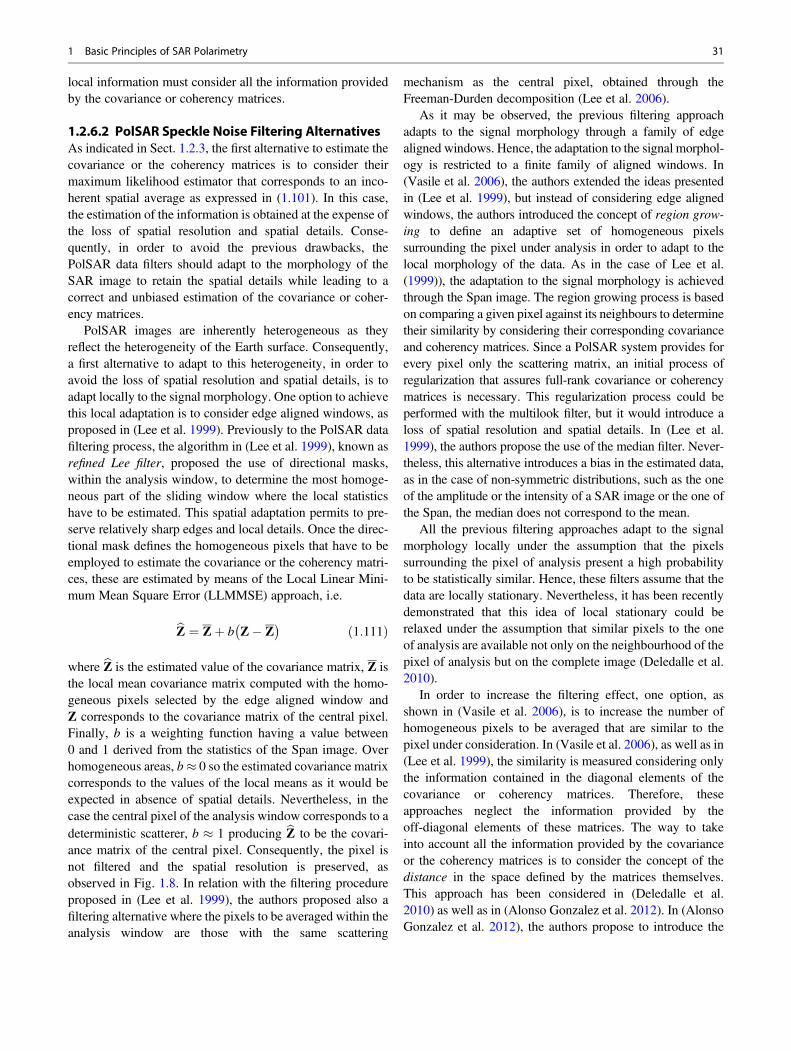
local information must consider all the information providedby the covariance or coherency matrices.

1.2.6.2 PolSAR Speckle Noise Filtering AlternativesAs indicated in Sect. 1.2.3, the first alternative to estimate thecovariance or the coherency matrices is to consider theirmaximum likelihood estimator that corresponds to an inco-herent spatial average as expressed in (1.101). In this case,the estimation of the information is obtained at the expense ofthe loss of spatial resolution and spatial details. Conse-quently, in order to avoid the previous drawbacks, thePolSAR data filters should adapt to the morphology of theSAR image to retain the spatial details while leading to acorrect and unbiased estimation of the covariance or coher-ency matrices.

PolSAR images are inherently heterogeneous as theyreflect the heterogeneity of the Earth surface. Consequently,a first alternative to adapt to this heterogeneity, in order toavoid the loss of spatial resolution and spatial details, is toadapt locally to the signal morphology. One option to achievethis local adaptation is to consider edge aligned windows, asproposed in (Lee et al. 1999). Previously to the PolSAR datafiltering process, the algorithm in (Lee et al. 1999), known asrefined Lee filter, proposed the use of directional masks,within the analysis window, to determine the most homoge-neous part of the sliding window where the local statisticshave to be estimated. This spatial adaptation permits to pre-serve relatively sharp edges and local details. Once the direc-tional mask defines the homogeneous pixels that have to beemployed to estimate the covariance or the coherency matri-ces, these are estimated by means of the Local Linear Mini-mum Mean Square Error (LLMMSE) approach, i.e.

bZ ¼ Zþ b Z� Z� � ð1:111Þ

where bZ is the estimated value of the covariance matrix, Z isthe local mean covariance matrix computed with the homo-geneous pixels selected by the edge aligned window andZ corresponds to the covariance matrix of the central pixel.Finally, b is a weighting function having a value between0 and 1 derived from the statistics of the Span image. Overhomogeneous areas, b� 0 so the estimated covariance matrixcorresponds to the values of the local means as it would beexpected in absence of spatial details. Nevertheless, in thecase the central pixel of the analysis window corresponds to adeterministic scatterer, b � 1 producing bZ to be the covari-ance matrix of the central pixel. Consequently, the pixel isnot filtered and the spatial resolution is preserved, asobserved in Fig. 1.8. In relation with the filtering procedureproposed in (Lee et al. 1999), the authors proposed also afiltering alternative where the pixels to be averaged within theanalysis window are those with the same scattering

mechanism as the central pixel, obtained through theFreeman-Durden decomposition (Lee et al. 2006).

As it may be observed, the previous filtering approachadapts to the signal morphology through a family of edgealigned windows. Hence, the adaptation to the signal morphol-ogy is restricted to a finite family of aligned windows. In(Vasile et al. 2006), the authors extended the ideas presentedin (Lee et al. 1999), but instead of considering edge alignedwindows, the authors introduced the concept of region grow-ing to define an adaptive set of homogeneous pixelssurrounding the pixel under analysis in order to adapt to thelocal morphology of the data. As in the case of Lee et al.(1999)), the adaptation to the signal morphology is achievedthrough the Span image. The region growing process is basedon comparing a given pixel against its neighbours to determinetheir similarity by considering their corresponding covarianceand coherency matrices. Since a PolSAR system provides forevery pixel only the scattering matrix, an initial process ofregularization that assures full-rank covariance or coherencymatrices is necessary. This regularization process could beperformed with the multilook filter, but it would introduce aloss of spatial resolution and spatial details. In (Lee et al.1999), the authors propose the use of the median filter. Never-theless, this alternative introduces a bias in the estimated data,as in the case of non-symmetric distributions, such as the oneof the amplitude or the intensity of a SAR image or the one ofthe Span, the median does not correspond to the mean.

All the previous filtering approaches adapt to the signalmorphology locally under the assumption that the pixelssurrounding the pixel of analysis present a high probabilityto be statistically similar. Hence, these filters assume that thedata are locally stationary. Nevertheless, it has been recentlydemonstrated that this idea of local stationary could berelaxed under the assumption that similar pixels to the oneof analysis are available not only on the neighbourhood of thepixel of analysis but on the complete image (Deledalle et al.2010).

In order to increase the filtering effect, one option, asshown in (Vasile et al. 2006), is to increase the number ofhomogeneous pixels to be averaged that are similar to thepixel under consideration. In (Vasile et al. 2006), as well as in(Lee et al. 1999), the similarity is measured considering onlythe information contained in the diagonal elements of thecovariance or coherency matrices. Therefore, theseapproaches neglect the information provided by theoff-diagonal elements of these matrices. The way to takeinto account all the information provided by the covarianceor the coherency matrices is to consider the concept of thedistance in the space defined by the matrices themselves.This approach has been considered in (Deledalle et al.2010) as well as in (Alonso Gonzalez et al. 2012). In (AlonsoGonzalez et al. 2012), the authors propose to introduce the


concept of binary partition tree (BPT) as a hierarchicalstructure to exploit the relations that may be establishedbetween similar pixels. In essence, the filtering alternativeproposed in (Alonso Gonzalez et al. 2012) produces first abinary partition tree that establishes the relations betweensimilar pixels on the basis of a distance that takes into accountall the polarimetric information. In a second step, the binarypartition tree is pruned to find the largest homogeneousregions of the image. This filtering alternative allows to filterlarge homogeneous areas while maintaining the spatialdetails of the data as observed in Fig. 1.9.

The objective of all the previous filtering techniques is toobtain the best estimate of the covariance or coherency matri-ces by means of increasing the number of averaged samples.Nevertheless, if the number of available homogeneous pixelsis not large enough, the way to improve the estimation of thecovariance and coherency matrices must be addressed byconsidering a better exploitation of the Wishart distribution.As shown in (Lopez Martínez and Fabregas 2003), theWishart distribution allows defining the multiplicative-additive speckle noise model for all the elements of thecovariance or the coherency matrices. This model has beenexploited for PolSAR data filtering in (Lopez Martínez andFabregas 2008), where it is demonstrated that if the filteringprocess is adapted to the multiplicative or additive nature ofspeckle, depending on the correlation of a pair of SARimages, it may lead to an improved estimation of the differentparametric parameters that characterize the covariance orcoherency matrices.

Beyond all the PolSAR data filtering techniques presentedin this section, there exist a wide variety of similarapproaches in the related literature, where a comparisonamong some of them has been presented in (Foucher et al.2012). Nevertheless, it may be concluded that reaching anoptimal compromise of a joint preservation of the polarimet-ric and the spatial information, in the case of PolSAR datafiltering, is still today a problem without an adequate solu-tion. Consequently, the selection of a particular filteringalternative for PolSAR data must take into consideration thefinal application of the PolSAR data in order to determine theoptimum filtering according to that application.

1.3 Polarimetric Scattering DecompositionTheorems

As shown in Sect. 1.1.2, the scattering matrix or the covari-ance and coherency matrices allow the characterization of ascatterer for a given frequency and a given imaging geome-try. The information provided by these matrices, at a particu-lar combination of transmitting and receiving polarizationstates, can be extended to any polarization state, thanks tothe concept of polarization synthesis. Nevertheless, whenfacing real polarimetric SAR data, the interpretation ofthese matrices is not straightforward due to the complexityof the scattering process and the high variability of thescatterers. Polarimetric decomposition techniques appear asa solution to interpret the information provided by the

Fig. 1.8 RADARSAT-2 polarimetric RGB image over San Francisco (USA) where the colour code is Shh blue, Svv red and Shv green. Filtered imagewith the LLMMSE speckle filter


scattering and the covariance and coherency matrices. Thesedecomposition techniques must be divided into two mainclasses. The first one, referred to as coherent polarimetricdecompositions, makes reference to those decompositiontechniques applied to the scattering matrix. The validity ofthese decomposition techniques is restricted to pointscatterers, that is, scatterers not affected by the specklenoise component. If applied to distributed scatterers, thesedecompositions would be random as they are not able to copewith the stochastic nature of the measurements. Distributedscatterers, on the contrary, can be analysed by the so-calledincoherent polarimetric decompositions that base the analysison the covariance or coherency matrices.

1.3.1 Coherent Scattering DecompositionTechniques

Section 1.1.2.1 introduced the 2 � 2 complex scatteringmatrix as a mathematical operator able to describe the scat-tering process that occurs when a wave reaches a givenscatterer. As indicated, this matrix contains the necessaryinformation to determine the far-field scattered wave by thescatterer as a function of the incident wave. Consequently,the scattering matrix characterizes the scatterer, for theemployed imaging geometry and the working frequency. Asindicated in Table 1.6, simple canonical scatteringmechanisms may be recognized from the scattering matrix.Nevertheless, in real measurements, the scattering matrix

usually presents a more complex structure that hinders theinterpretation in physical terms. The objective behind coher-ent scattering decomposition techniques is to decompose themeasured scattering matrix by the SAR system, i.e. S, as acombination of the scattering matrices corresponding to sim-pler scatterers:

S ¼Xki¼1

ciSi: ð1:112Þ

In (1.157), the symbol Si corresponds to the response ofevery one of the simple or canonical scatterers, whereas thecomplex coefficients ci indicate the weight of Si in the com-bination leading to the measured S. As observed in (1.112),the term combination refers to the weighted addition of thek scattering matrices. In order to simplify the understandingof (1.112), but also with the objective to make possible thedecomposition itself, it is desirable that the matrices Si pres-ent the property of independence among them to avoid aparticular scattering behaviour to appear in more than onematrix Si. Often, the independence condition is substituted bythe most restrictive property of orthogonality of thecomponents Si. Orthogonality helps to eliminate possibleambiguities in the decomposition of the scattering matrix inthose cases in which the elements Si are not orthogonal.

The scattering matrix S characterizes the scattering pro-cess produced by a given scatterer and therefore the scattereritself. This is possible only in those cases in which both the

Fig. 1.9 RADARSAT-2 polarimetric RGB image over San Francisco (USA) where the colour code is Shh blue, Svv red and Shv green. Filtered imagewith the BPT speckle filter


incident and the scattered waves are completely polarizedwaves. Consequently, coherent scattering decompositionscan be only employed to study the so-called coherentscatterers. These scatterers are also known as point or puretargets.

In a real situation, the measured scattering matrix by theradar S corresponds to a complex coherent scatterer. Only insome occasions, this matrix will correspond to a simpler orcanonical object, in which a good example is, for instance,the trihedrals employed to calibrate SAR imagery. Othersimple scattering mechanisms may be observed inTable 1.6. Nevertheless, in a general situation, a direct analy-sis of the matrix S, with the objective to infer the physicalproperties of the scatterer under study, is shown to be com-plex. Consequently, the physical properties of the targetunder study are extracted and interpreted through the analysisof the simpler responses Si and the corresponding complexcoefficients ci in (1.112).

The decomposition exposed in (1.112) is not unique in thesense that it is possible to find a number of infinite sets{Si; i ¼ 1, . . ., k} in which the matrix S can be decomposed.Nevertheless, only some of the sets {Si; i ¼ 1, . . ., k} areconvenient in order to interpret the information contained inS. Two examples of these decomposition bases have beenalready shown in Sect. 1.1.2.2. Other examples of coherentscattering decompositions are the Krogager (Krogager 1990)or the Cameron decompositions (Cameron and Leung 1990).

1.3.1.1 The Pauli DecompositionThe most relevant coherent scattering decomposition is thePauli decomposition that was already introduced in Sect.1.1.2.2. The Pauli decomposition expresses the measuredscattering matrix S in the so-called Pauli basis. If we consid-

ered the conventional orthogonal linear basis bh, bv,n o, in a

general case, the Pauli basis {Sa, Sb, Sc, Sd} is given by thefollowing four 2 � 2 matrices:

Sa ¼ 1ffiffiffi2

p 1 0

0 1

� �ð1:113Þ

Sb ¼ 1ffiffiffi2

p 1 0

0 �1

� �ð1:114Þ

Sc ¼ 1ffiffiffi2

p 0 1

1 0

� �ð1:115Þ

Sd ¼ 1ffiffiffi2

p 0 �1

1 0

� �: ð1:116Þ

Asmentioned, it has been always considered that Shv¼ Svh,since reciprocity applies in a monostatic system configuration

under the BSA convention. In this situation, the Pauli basiscan be reduced to a basis composed by the matrices (1.113),(1.114) and (1.115), that is, {Sa, Sb, Sc}. Consequently,given a measured scattering matrix S, this matrix can beexpressed as follows:

S ¼ Shh ShvShv Svv

� �¼ aSa þ bSb þ cSc ð1:117Þ

where the complex coefficients that determine the contribu-tion of every component of the basis can be obtained as

a ¼ Shh þ Svvffiffiffi2

p , b ¼ Shh � Svvffiffiffi2

p , c ¼ffiffiffi2

pShv ð1:118Þ

From the previous equations, it can be shown that

SPAN Sð Þ ¼ aj j2 þ bj j2 þ cj j2: ð1:119Þ

The interpretation of the Pauli decomposition must bedone according to the matrices {Sa, Sb, Sc} and theircorresponding decomposition coefficients, i.e. {a, b, c}. InSect. 1.1.2.1 it was seen that the matrices {Sa, Sb, Sc} corre-spond to the scattering behaviour of some canonical bodies.

The matrix Sa corresponds to the scattering matrix of asphere, a plate or a trihedral; see Table 1.6. Generally, Sa isreferred to as single- or odd-bounce scattering. Hence, thecomplex coefficient a represents the contribution of Sa to thefinal measured scattering matrix. In particular, the intensity ofthis coefficient, i.e. |a|2, determines the power scattered byscatterers characterized by single- or odd-bounce.

The second matrix Sb represents the scattering mechanismof a dihedral oriented at 0 degrees; see Table 1.6. In general,this component indicates a scattering mechanismcharacterized by double- or even-bounce, since the polariza-tion of the returned wave is mirrored with respect to the oneof the incident wave. Consequently, b stands for the complexcoefficient of this scattering mechanism, and |b|2 representsthe scattered power by this type of targets.

Finally, the third matrix Sc corresponds to the scatteringmechanism of a diplane oriented at 45 degrees. As it can beobserved in (1.115), and considering that this matrix is

expressed in the linear orthogonal basis bh, bv,n o, the

scatterer returns a wave with a polarization orthogonal tothe one of the incident wave. From a qualitative point ofview, the scattering mechanism represented by Sc is referredto those scatterers which are able to return the orthogonalpolarization, from which one of the best examples is thevolume scattering produced by the forest canopy. The com-plex scattering that occurs in the forest canopy, characterizedby multiple reflections, makes possible to return energy onthe orthogonal polarization, with respect to the polarization


of the incident wave. Consequently, this third scatteringmechanism is usually referred to as volume scattering. Thecoefficient c represents the contribution of Sc to S, whereas |c|2 stands for the scattered power by this type of scatters.

The Pauli decomposition of the scattering matrix is oftenemployed to represent the polarimetric information in a sin-gle SAR image. The polarimetric information of S could berepresented with the combination of the intensities |Shh|

2, |Svv|

2 and 2|Shv|2 in a single RGB image, i.e. each of the

previous intensities coded as a colour channel. The maindrawback of this approach is the physical interpretation ofthe resulting image in terms of |Shh|

2, |Svv|2 and 2|Shv|

2.Consequently, a RGB image can be created with theintensities |a|2, |b|2 and |c|2, which, as indicated previously,correspond to clear physical scattering mechanisms. Thus,the resulting colour image can be employed to interpret thephysical information from a qualitative point of view. Themost employed codification corresponds to

aj j2 ! Blue, bj j2 ! Red, cj j2 ! Green: ð1:120Þ

Then, the resulting colour of the RGB image is interpretedin terms of scattering mechanism as given in (1.113)–(1.115);see Fig. 1.10.

1.3.2 Incoherent Scattering DecompositionsTechniques

As explained in the previous sections, the scattering matrixS is only able to characterize the point or deterministic

scatterers. In this case, the scattering process is completelydetermined by the five independent parameters the matrixS may present. On the contrary, this matrix cannot beemployed to characterize, from a polarimetric point of view,the distributed scatterers, as the five independent parametersof the S matrix are insufficient to characterize the scatteringprocess. As detailed in Sect. 1.2, distributed scatterers can beonly characterized statistically due to the presence of specklenoise by means of higher-order descriptors. Since specklenoise must be reduced, only second-order polarimetricrepresentations can be employed to analyse distributedscatterers. In the case of monostatic scattering under theBSA convention, these second-order descriptors are the3 � 3 Hermitian covariance C or coherency T matrices.

The complexity of the scattering process makes extremelydifficult the physical study of a given scatterer through thedirect analysis of C or T. Hence, the objective of the incoher-ent decompositions is to separate the C or T matrices as thecombination of second-order descriptors corresponding tosimpler or canonical objects, presenting an easier physicalinterpretation. These decomposition theorems can beexpressed as

C ¼Xki¼1

piCi,T ¼Xki¼1

qiTi ð1:121Þ

where the canonical responses are represented by Ci and Ti

and pi and qi denote the coefficients of these components inC or T, respectively. As in the case of the coherentdecompositions, it is desirable that these components presentsome properties. First of all, it is desirable that the

Fig. 1.10 RADARSAT-2 polarimetric RGB-Pauli image over San Francisco (USA) where the colour code is |Shh + Svv|2 blue, |Shh � Svv|

2 red and2|Shv|

2 green


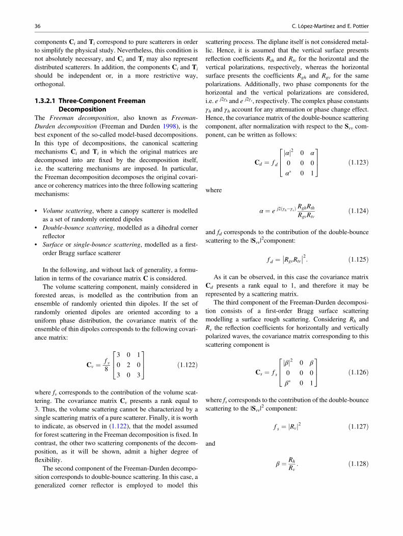
components Ci and Ti correspond to pure scatterers in orderto simplify the physical study. Nevertheless, this condition isnot absolutely necessary, and Ci and Ti may also representdistributed scatterers. In addition, the components Ci and Ti

should be independent or, in a more restrictive way,orthogonal.

1.3.2.1 Three-Component FreemanDecomposition

The Freeman decomposition, also known as Freeman-Durden decomposition (Freeman and Durden 1998), is thebest exponent of the so-called model-based decompositions.In this type of decompositions, the canonical scatteringmechanisms Ci and Ti in which the original matrices aredecomposed into are fixed by the decomposition itself,i.e. the scattering mechanisms are imposed. In particular,the Freeman decomposition decomposes the original covari-ance or coherency matrices into the three following scatteringmechanisms:

• Volume scattering, where a canopy scatterer is modelledas a set of randomly oriented dipoles

• Double-bounce scattering, modelled as a dihedral cornerreflector

• Surface or single-bounce scattering, modelled as a first-order Bragg surface scatterer

In the following, and without lack of generality, a formu-lation in terms of the covariance matrix C is considered.

The volume scattering component, mainly considered inforested areas, is modelled as the contribution from anensemble of randomly oriented thin dipoles. If the set ofrandomly oriented dipoles are oriented according to auniform phase distribution, the covariance matrix of theensemble of thin dipoles corresponds to the following covari-ance matrix:

Cv ¼ f v8

3 0 1

0 2 0

3 0 3

264375 ð1:122Þ

where fv corresponds to the contribution of the volume scat-tering. The covariance matrix Cv presents a rank equal to3. Thus, the volume scattering cannot be characterized by asingle scattering matrix of a pure scatterer. Finally, it is worthto indicate, as observed in (1.122), that the model assumedfor forest scattering in the Freeman decomposition is fixed. Incontrast, the other two scattering components of the decom-position, as it will be shown, admit a higher degree offlexibility.

The second component of the Freeman-Durden decompo-sition corresponds to double-bounce scattering. In this case, ageneralized corner reflector is employed to model this

scattering process. The diplane itself is not considered metal-lic. Hence, it is assumed that the vertical surface presentsreflection coefficients Rth and Rtv for the horizontal and thevertical polarizations, respectively, whereas the horizontalsurface presents the coefficients Rgh and Rgv for the samepolarizations. Additionally, two phase components for thehorizontal and the vertical polarizations are considered,i.e. e j2γh and e j2γv, respectively. The complex phase constantsγh and γh account for any attenuation or phase change effect.Hence, the covariance matrix of the double-bounce scatteringcomponent, after normalization with respect to the Svv com-ponent, can be written as follows:

Cd ¼ f d

αj j2 0 α

0 0 0

α� 0 1

264375 ð1:123Þ

where

α ¼ e j2 γh�γvð Þ RghRth

RgvRtvð1:124Þ

and fd corresponds to the contribution of the double-bouncescattering to the |Svv|

2component:

f d ¼ RgvRtv

�� 2: ð1:125Þ

As it can be observed, in this case the covariance matrixCd presents a rank equal to 1, and therefore it may berepresented by a scattering matrix.

The third component of the Freeman-Durden decomposi-tion consists of a first-order Bragg surface scatteringmodelling a surface rough scattering. Considering Rh andRv the reflection coefficients for horizontally and verticallypolarized waves, the covariance matrix corresponding to thisscattering component is

Cs ¼ f s

βj j2 0 β

0 0 0

β� 0 1

264375 ð1:126Þ

where fs corresponds to the contribution of the double-bouncescattering to the |Svv|

2 component:

f s ¼ Rvj j2 ð1:127Þ

and

β ¼ Rh

Rv: ð1:128Þ


As in the case for the double-bounce scattering mecha-nism, Cs presents a rank equal to 1.

Finally, it can be seen that the Freeman decompositionexpresses the measured covariance matrix C as

C ¼ Cv þ Cd þ Cs ð1:129Þ

that takes the expression

C ¼

3 f v8

þ f d αj j2 þ f s βj j2 0f v8

þ f dαþ f sβ

02 f v8

0

f v8

þ f dα� þ f sβ

� 03 f v8

þ f d þ f s

2666664

3777775:ð1:130Þ

As one may deduce from (1.130), the Freeman decompo-sition presents five independent parameters {fv, fd, fs, α, β}but only four equations. Consequently, some hypothesis mustbe considered in order to find the values of {fv, fd, fs, α, β}.Considering that the Span of the covariance matrix may beexpressed as a function of the power scattered by each com-ponent of the decomposition {Cv, Cd, Cs}, i.e.

SPAN Cð Þ ¼ Shhj j2 þ Svvj j2 þ 2 Shvj j2¼ Pv þ Pd þ Ps ð1:131Þ

the term Pv corresponds to the contribution of the volumescattering of the final covariance matrix C. Hence, thescattered power by this component may be written as

Pv ¼ f v: ð1:132Þ

The power scattered by the double-bounce component isexpressed as

Pd ¼ f d 1þ αj j2� �

, ð1:133Þ

whereas the power scattered by the surface component is

Ps ¼ f s 1þ βj j2� �

: ð1:134Þ

Consequently, the scattered power at each component{Pv, Pd, Ps} may be employed to generate a RGB image,similarly as in the case of the Pauli decomposition, to presentall the colour-coded polarimetric information in a uniqueimage; see Fig. 1.11.

1.3.2.2 Four-Component YamaguchiDecomposition

As it may be observed in (1.130), the three-component Free-man decomposition is based on the assumption that theanalysed scatterer presents reflection symmetry, that is, thecorrelation of the co-polar channels, either Shh or Svv, with thecross-polar one Shv is zero, that is, E ShhS

�hv

¼ 0 andE ShvS

�vv

¼ 0 . This type of symmetry in the scatteringprocess appears normally in the case of natural distributedscatterers such as forests or grassland areas. Nevertheless, inthe case of more complex scattering scenarios, for instance,man-made scatterers, this assumption is no longer true. Inaddition to the previous limitation, the Freeman decomposi-tion, as detailed in the previous section, considers only onetype of volume scattering, as reflected in (1.122), where thescattering at the co-polar channels are supposed equal, i.e. E{|Shh|

2} ¼ E{|Svv|2}. The four-component Yamaguchi decom-

position is proposed to overcome the previous two limitationsof the Freeman decomposition (Yamaguchi et al. 2005).

If one considers the canonical scattering mechanismspresented in Table 1.6, it may be observed that only therotated thin cylinder or the right- and left-handed helices areable to produce a covariance matrix such that E ShhS

�hv

6¼ 0and E ShvS

�vv

6¼ 0 and therefore produce a covariancematrix without reflection symmetry. In the four-componentYamaguchi decomposition, the authors propose to take intoaccount the absence of this type of symmetry by consideringfirst the three scattering mechanisms considered by the Free-man decomposition, that is, volume, double-bounce and sur-face scattering, together with a fourth component composedby either the left- or the right-handed helix scattering(Krogager 1990). In particular, the helix scattering ischaracterized by generating a left-handed or a right-handedcircular polarization for all incident linear polarizations,according to the scatterer helicity. The left-handed helix,whose scattering matrix is presented in Table 1.6, leads tothe following covariance matrix:

Clh ¼ f c4

1 �jffiffiffi2

p �1

jffiffiffi2

p2 �j

ffiffiffi2

p

�1 jffiffiffi2

p1

264375 ð1:135Þ

whereas the right-handed helix results in the followingcovariance matrix:

Crh ¼ f c4

1 jffiffiffi2

p �1

�jffiffiffi2

p2 j

ffiffiffi2

p

�1 �jffiffiffi2

p1

264375 ð1:136Þ


where fc accounts for the contribution of the helix compo-nent. As it may be observed in the previous two matrices, theinclusion of the helix component allows to consider a scatter-ing mechanism without reflection symmetry. The selection ofthe left- or the right-handed helix will be determined by thesign of the imaginary part of E ShhS

�hv

or E ShvS

�vv

.

In order to model the volume scattering, the Freemandecomposition considered a set of randomly oriented dipoles,oriented according to a uniform phase distribution. Neverthe-less, when confronted to a real forest, the effect of the trunkand the branches, especially at high frequencies, may lead toa scattering from a cloud of oriented dipoles but with anon-uniform distribution. In this case, depending on themain orientation of these thin dipoles, the power associatedwith E{|Shh|

2} and E{|Svv|2} may be different if the dipoles

are preferably oriented horizontally or vertically, respec-tively. As it may be seen, the volume model considered bythe Freeman decomposition (1.122) cannot take into accountthis effect. In order to account for this preference in theorientation, instead of considering a uniform distribution forthe orientation of the thin dipoles, it is proposed to considerthe following distribution:

p θð Þ ¼12cos θ for θj j < π=2

0 for θj j > π=2

8<: ð1:137Þ

where θ is taken from the horizontal axis seen from the radar.When considering a cloud of randomly oriented, very thinhorizontal dipoles, the volume scattering is represented bythe following scattering matrix:

Cv ¼ f v15

8 0 2

0 4 0

2 0 3

264375: ð1:138Þ

Otherwise, if the cloud of thin dipoles is considered to becomposed of vertical dipoles, the covariance matrixrepresenting the volume component is

Cv ¼ f v15

3 0 2

0 4 0

2 0 8

264375: ð1:139Þ

Fig. 1.11 Freeman decomposition of the RADARSAT-2 polarimetric RGB-Pauli image over San Francisco (USA). Top panel, from left to right:Pd, Pv, Ps. Bottom panel: RGB composition with Pd red, Pv green and Ps blue


In all the cases, fv corresponds to the contribution of thevolume scattering.

Allowing the volume scattering to depend on the mainorientation of the particles makes it necessary to introduce anadditional step in the decomposition able to select the volumescattering most adapted to the data under observation. Thefour-component Yamaguchi decomposition proposes toselect among (1.122), (1.138) and (1.139) according to theratio χ ¼ 10 log (E{|Svv|

2}/E{|Shh|2}). Table 1.7 details the

procedure to select the type of volume scattering proposed in(Yamaguchi et al. 2005).

Finally, the double-bounce and the surface scatteringcomponents of the four-component Yamaguchi decomposi-tion are the same as the Freeman decomposition. Conse-quently, the Yamaguchi decomposition models thecovariance matrix as

C ¼

f c4

þ f d αj j2 þ f s βj j2 �j

ffiffiffi2

pf c

4� f c

4þ f dαþ f sβ

∓j

ffiffiffi2

pf c

4f c2

�j

ffiffiffi2

pf c

4

� f c4

þ f dα� þ f sβ

� ∓j

ffiffiffi2

pf c

4f c4

þ f d þ f s

26666664

37777775

þ f v

a 0 d

0 b 0

d 0 c

264375

ð1:140Þ

where the last matrix accounts for the volume scattering thathas been selected according to Table 1.7. As one may deducefrom (1.140), the four-component Yamaguchi decompositionpresents six independent parameters {fv, fd, fs, fc, α, β}.Considering that the Span of the covariance matrix may beexpressed as a function of the power scattered by each com-ponent of the decomposition {Cv, Cd, Cs, Clh/rh}, i.e.

SPAN Cð Þ ¼ Shhj j2 þ Svvj j2 þ 2 Shvj j2¼ Pv þ Pd þ Ps þ Pc ð1:141Þ

the term Pv corresponds to the contribution of the volumescattering of the final covariance matrix C. Hence, thescattered power by this component may be written as

Pv ¼ f v, ð1:142Þ

the power scattered by the double-bounce component isexpressed as

Pd ¼ f d 1þ αj j2� �

, ð1:143Þ

the power scattered by the surface component is

Ps ¼ f s 1þ βj j2� �

, ð1:144Þ

whereas the power scattered by the helix component is

Pc ¼ f c: ð1:145Þ

Consequently, the scattered power at each component{Pv, Pd, Ps, Pc} may be combined to generate a RGBimage similarly as in the case of the Pauli decomposition, topresent all the colour-coded polarimetric information in aunique image; see Fig. 1.12.

1.3.2.3 Non-negative Eigenvalue DecompositionAs indicated in the previous two sections, both the Freeman-Durden and the Yamaguchi decomposition work under thehypothesis that the measured covariance matrix may bedecomposed as the sum of a set of scattering mechanisms.Whereas the first decomposition assumes reflection symme-try for the scattering medium, this limitation is addressed bythe second one by considering a fourth scattering componentrepresented by either the left- or the right-handed helix scat-tering. All the scattering mechanisms in which the measuredcovariance matrix is decomposed into are represented bytheir corresponding covariance matrices. As shown in (VanZyl et al. 2011), these matrices should correspond to physicalscattering mechanisms, so all their eigenvalues must be largerthan or equal to zero; in other words, the power received byany combination of transmitting and receiving polarizationsshould never be negative.

A close analysis of the Freeman-Durden decompositionshows that the contribution of the volume scattering compo-nent is directly estimated from the cross-polarized term, thatis, the decomposition assumes that neither the double-bouncenor the surface scattering components contribute to it. Thisassumption is very strict as, for instance, the rotation of thepolarization basis of the scattering matrix due to terrainslopes in the along-track dimension (Lee et al. 2002) oreven rough surfaces may lead to significant cross-polarizedpower (Hajnsek et al. 2003). Consequently, if these effectsare not taken into account, they may produce an overestima-tion of the volume component. Once this volume componentis estimated from the data, it is extracted from the measured

Table 1.7 Selection of the volume scattering covariance matrix

χ < � 2 dB �2 dB < χ < 2 dB χ > 2 dB

Cv ¼ f v15

8 0 2

0 4 0

2 0 3

264375 Cv ¼ f v

8

3 0 1

0 2 0

3 0 3

264375 Cv ¼ f v

15

3 0 2

0 4 0

2 0 8

264375


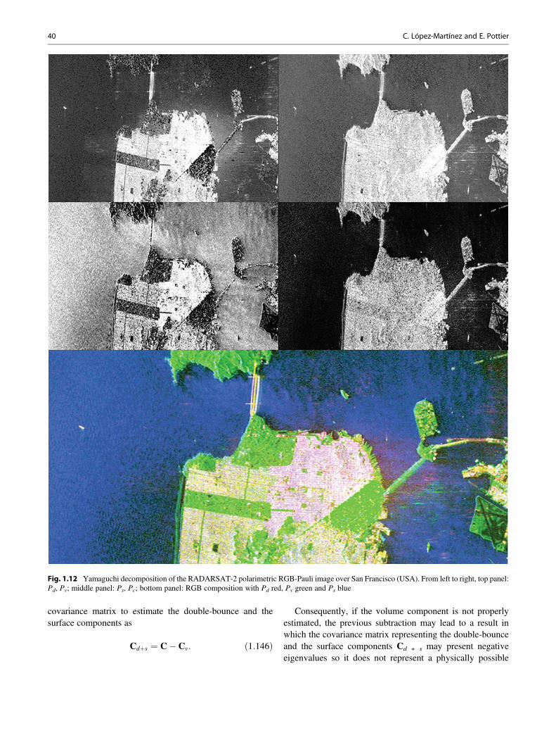
covariance matrix to estimate the double-bounce and thesurface components as

Cdþs ¼ C� Cv: ð1:146Þ

Consequently, if the volume component is not properlyestimated, the previous subtraction may lead to a result inwhich the covariance matrix representing the double-bounceand the surface components Cd + s may present negativeeigenvalues so it does not represent a physically possible

Fig. 1.12 Yamaguchi decomposition of the RADARSAT-2 polarimetric RGB-Pauli image over San Francisco (USA). From left to right, top panel:Pd, Pv; middle panel: Ps, Pc; bottom panel: RGB composition with Pd red, Pv green and Ps blue


scattering mechanism. The Yamaguchi decomposition alsopresents this drawback as the double-bounce and the surfacelike scattering components are estimated after the subtractionof the volume scattering component.

In order to correct the presence of negative eigenvalueswhen considering a decomposition based on (1.146), van Zylet al. (Van Zyl et al. 2011) proposed the non-negative eigen-value decomposition (NNED). The Freeman-Durden and theYamaguchi decompositions assume that the measuredcovariance matrix results from the addition of a set of scatter-ing mechanisms. Nevertheless, the NNED approach pro-posed to decompose the measured covariance matrix as

C ¼ aCmodel þ Cremainder: ð1:147Þ

The matrix Cmodel represents the covariance matrixpredicted by a theoretical model, for instance, the volumescattering component. The parameter a is introduced in(1.147) to assure that all the matrices in (1.147) represent

physically realizable scattering mechanism. Finally, the sec-ond matrixCremainder will contain whatever is in the measuredmatrix C that is not consistent with the model matrix Cmodel.

To find the value of a, (1.147) may be written as

Cremainder ¼ C� aCmodel: ð1:148Þ

Consequently, the value of a must assure that theeigenvalues of Cremainder must be positive. In the case of ascattering media with reflection symmetry, (1.147) may bewritten as

Cremainder ¼ξ 0 ρ

0 η 0

ρ� 0 ζ

264375� a

ξa 0 ρa0 ηa 0

ρ�a 0 ζa

264375: ð1:149Þ

Therefore, the maximum value of a that assures that theeigenvalues of Cremainder are positive corresponds to

amax ¼ min η=ηa,1

2 ξaζa � ρaj j2� � Z �

ffiffiffiffiffiffiffiffiffiffiffiffiffiffiffiffiffiffiffiffiffiffiffiffiffiffiffiffiffiffiffiffiffiffiffiffiffiffiffiffiffiffiffiffiffiffiffiffiffiffiffiffiffiffiffiffiffiffiffiZ2 � 4 ξaζa � ρaj j2

� �ξζ � ρj j2

r� �8<:9=;, ð1:150Þ

where Z ¼ ξζa þ ζξað Þ � ρρ�a � ρ�ρa. For the case of scatter-ing media not presenting reflection symmetry, the process toderive the maximum value of a is similar, but results in morecomplex expressions.

The volume scattering model employed for the canopyscattering is based on a cosine-squared distribution raised tothe nth power for the vegetation orientation (Arii et al. 2011).Considering that the basic scatterer in the canopy is a dipole,it was shown that the covariance matrix can be written as

Cv θ0, σð Þ ¼ Cα þ p σð ÞCβ þ q σð ÞCγ ð1:151Þ

where

Cα ¼ 18

3 0 1

0 2 0

3 0 3

264375, ð1:152Þ

Cβ ¼ 18

��2 cos 2θ0

ffiffiffi2

pcos 2θ0 0ffiffiffi

2p

cos 2θ0 0ffiffiffi2

pcos 2θ0

0ffiffiffi2

pcos 2θ0 2 cos 2θ0

264375,ð1:153Þ

Cγ ¼ 18

�cos 4θ0 � ffiffiffi

2p

cos 4θ0 � cos 4θ0� ffiffiffi

2p

cos 4θ0 �2 cos 4θ0ffiffiffi2

pcos 4θ0

� cos 4θ0ffiffiffi2

pcos 4θ0 cos 4θ0

264375,

ð1:154Þ

and

p σð Þ ¼ 2:0806σ6‐6:3350σ5

þ 6:3864σ4‐0:4431σ3‐3:9638σ2‐0:0008σþ 2:000, ð1:155Þ

q σð Þ ¼ 9:0166σ6‐18:7790σ5 þ 4:9590σ4

þ 14:5629σ3‐10:8034σ2‐0:1902σþ 1:000: ð1:156Þ

In the previous equations, the parameter θ0 represents themean orientation angle of the thin dipoles, whereas σaccounts for the randomness of the cloud of dipoles.

On the basis of the previous procedure to avoid the extrac-tion of non-physical covariance matrices, Arii et al. (Ariiet al. 2011) proposed an adaptive NNED decomposition


theorem, where also the previous extended model for volumescattering is considered. According to the NNED decompo-sition, a covariance matrix for the volume scattering is firstsubtracted from the measured covariance matrix as follows:

Cremainder ¼ C� f vCv θ0, σð Þ: ð1:157Þ

As indicated previously, fv can be obtained analyticallyonly under the assumption of reflection symmetry. In thosecases in which the previous hypothesis does not apply, themaximum value of fv is obtained numerically by calculatingthe eigenvalues Cremainder at specific randomness σ and meanorientation angle θ0 by varying fv, and then, the maximum fvin which all three eigenvalues of Cremainder are nonnegative isselected. Once the volume component is extracted from themeasured covariance matrix as specified in (1.157), theremainder matrix can be written as

C� f vCv θ0, σð Þ ¼ f dCd þ f sCs þ C0remainder ð1:158Þ

where in this case Cd and Cs correspond to the double-bounce and surface scattering mechanisms already employed

in the three-component Freeman-Durden decomposition. Theparameters fd, fs and C0

remainder are obtained through an eigen-value decomposition. This procedure shows how to find theparameters in the decomposition for a specific pair ofrandomness σ and mean orientation angle θ0. To find thebest fit decomposition, the power in the remainder matrixfor all pairs of randomness and mean orientation angles isevaluated and then the set of parameters that minimize thepower associated with C0

remainder should be found.Finally, the scattered power at each component {fv, fd, fs}

may be combined to generate a RGB image similarly as in thecase of the Pauli decomposition, to present all the colour-coded polarimetric information in a unique image; seeFig. 1.13.

1.3.2.4 Eigenvector-Eigenvalue-BasedDecomposition

The previous incoherent decompositions were constructed onthe assumption that the scattering of a given pixel was due tothe combination of some predefined scattering mechanisms,hence assuming different properties of the scattering pro-cesses. These assumptions make these decompositions to be

Fig. 1.13 Van Zyl decomposition of the RADARSAT-2 polarimetric RGB-Pauli image over San Francisco (USA). Top panel, from left to right: fd,fv, fs. Bottom panel: RGB composition with fd red, fv green and fs blue


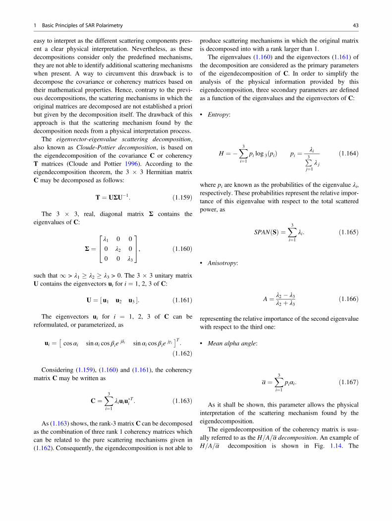
easy to interpret as the different scattering components pres-ent a clear physical interpretation. Nevertheless, as thesedecompositions consider only the predefined mechanisms,they are not able to identify additional scattering mechanismswhen present. A way to circumvent this drawback is todecompose the covariance or coherency matrices based ontheir mathematical properties. Hence, contrary to the previ-ous decompositions, the scattering mechanisms in which theoriginal matrices are decomposed are not established a prioribut given by the decomposition itself. The drawback of thisapproach is that the scattering mechanism found by thedecomposition needs from a physical interpretation process.

The eigenvector-eigenvalue scattering decomposition,also known as Cloude-Pottier decomposition, is based onthe eigendecomposition of the covariance C or coherencyT matrices (Cloude and Pottier 1996). According to theeigendecomposition theorem, the 3 � 3 Hermitian matrixC may be decomposed as follows:

T ¼ UΣU�1: ð1:159Þ

The 3 � 3, real, diagonal matrix Σ contains theeigenvalues of C:

Σ ¼λ1 0 0

0 λ2 0

0 0 λ3

264375, ð1:160Þ

such that 1 > λ1 λ2 λ3 > 0. The 3 � 3 unitary matrixU contains the eigenvectors ui for i ¼ 1, 2, 3 of C:

U ¼ u1 u2 u3½ �: ð1:161Þ

The eigenvectors ui for i ¼ 1, 2, 3 of C can bereformulated, or parameterized, as

ui ¼ cos αi sin αi cos βiejδi sin αi cos βie

jγi� �T

:

ð1:162Þ

Considering (1.159), (1.160) and (1.161), the coherencymatrix C may be written as

C ¼X3i¼1

λiuiu�Ti : ð1:163Þ

As (1.163) shows, the rank-3 matrixC can be decomposedas the combination of three rank 1 coherency matrices whichcan be related to the pure scattering mechanisms given in(1.162). Consequently, the eigendecomposition is not able to

produce scattering mechanisms in which the original matrixis decomposed into with a rank larger than 1.

The eigenvalues (1.160) and the eigenvectors (1.161) ofthe decomposition are considered as the primary parametersof the eigendecomposition of C. In order to simplify theanalysis of the physical information provided by thiseigendecomposition, three secondary parameters are definedas a function of the eigenvalues and the eigenvectors of C:

• Entropy:

H ¼ �X3i¼1

pi log 3 pið Þ pi ¼ λiP3j¼1

λ j

ð1:164Þ

where pi are known as the probabilities of the eigenvalue λi,respectively. These probabilities represent the relative impor-tance of this eigenvalue with respect to the total scatteredpower, as

SPAN Sð Þ ¼X3i¼1

λi: ð1:165Þ

• Anisotropy:

A ¼ λ2 � λ3λ2 þ λ3

ð1:166Þ

representing the relative importance of the second eigenvaluewith respect to the third one:

• Mean alpha angle:

α ¼X3i¼1

piαi: ð1:167Þ

As it shall be shown, this parameter allows the physicalinterpretation of the scattering mechanism found by theeigendecomposition.

The eigendecomposition of the coherency matrix is usu-ally referred to as the H=A=α decomposition. An example ofH=A=α decomposition is shown in Fig. 1.14. The


interpretation of the information provided by theeigendecomposition of the coherency matrix must beperformed in terms of the eigenvalues and eigenvectors ofthe decomposition or in terms of H=A=α. Nevertheless, bothinterpretations have to be considered as complementary.

The interpretation of the scattering mechanisms given bythe eigenvectors of the decomposition, ui for i ¼ 1, 2, 3, isperformed by means of a mean dominant mechanism whichcan be defined as follows:

u0 ¼ cos α sin α cos βe jδ sin α cos βe jγh iT

, ð1:168Þ

where the remaining average angles β, δ, γ are defined in thesame way as α.

The study of the mechanism given in (1.168) is mainlyperformed through the interpretation of the mean alpha angleα, since its value can be easily related to the physics behindthe scattering process. The next list details the interpretationof α:

• α ! 0: the scattering corresponds to single-bounce scat-tering produced by a rough surface.

• α ! π=4: the scattering mechanism corresponds to vol-ume scattering.

• α ! π=2 : the scattering mechanism is due to double-bounce scattering.

The second part in the interpretation of the eigendecom-position is performed by studying the value of theeigenvalues of the decomposition. A given eigenvaluecorresponds to the associated scattered power to thecorresponding eigenvector. Consequently, the value of theeigenvalue gives the importance of the corresponding eigen-vector or scattering mechanism. The ensemble of scatteringmechanisms is studied by means of the entropy H and theanisotropy A. The Entropy H determines the degree ofrandomness of the scattering process, which can be alsointerpreted as the degree of statistical disorder. In this way

• H ! 0:

λ1 ¼ SPAN, λ2 ¼ 0, λ3 ¼ 0 ð1:169Þ

As observed, in this case, the covariance matrixC presentsrank 1, and the scattering process corresponds to a purescatterer.

• H ! 1:

λ1 ¼ λ2 ¼ λ3 ¼ SPAN3

: ð1:170Þ

In this situation, the covariance matrix C presents rank3, that is, the scattering process is due to the combination ofthree pure targets. Consequently, C corresponds to theresponse of a distributed target. For instance, volumescattering for a forest canopy presents an entropy valuevery close to 1.

• 0 < H < 1: In this case, the final scattering mechanismgiven by C results from the combination of the three puretargets given by ui for i ¼ 1, 2, 3, but weighted by thecorresponding eigenvalue.

The anisotropy A, (1.166), is a parameter complementaryto the entropy. The anisotropy measures the relative impor-tance of the second and the third eigenvalues of theeigendecomposition. From a practical point of view, theanisotropy can be employed as a source of discriminationonly when H > 0.7. The reason is that for lower entropies, thesecond and third eigenvalues are highly affected by the SARsystem noise.

In relation with the previous parameters, the Shannonentropy (SE) was introduced in (Morio et al. 2007):

SE ¼ log π3e3 Tj j� � ¼ SEI þ SEP ð1:171Þ

as the sum of two terms. The term SEI is the intensitycontribution that depends on the total power

SEI ¼ 3 logπ � e � I

3

� �¼ 3 log

π � e � trace Τð Þ3

� �ð1:172Þ

whereas SEP is the polarimetric contribution

SEP ¼ log 27Τj j

trace Τð Þ½ �3 !

: ð1:173Þ

As indicated in Sect. 1.1.2.5, for some particularconfigurations, a polarimetric SAR system may not measurethe complete polarimetric information. In this simpler config-uration of dual polarization, the radar transmits only a singlepolarization and receives, either coherently or incoherently,two orthogonal components of the scattered signal. In thisconfiguration, the covariance C and coherency Tmatrices are2 � 2 Hermitian matrices. As it has been demonstrated(Cloude 2007a), these reduced matrices can be decomposedalso considering their eigendecompositions. The sole partic-ularity is that in this situation the matrices present only twoeigenvalues.

1.3.2.5 The Touzi Target ScatteringDecompositions

The Touzi decomposition (Touzi 2007) was introduced as anextension of the Kennaugh-Huynen coherent target scattering


Fig. 1.14 H=A=α decomposition of the RADARSAT-2 polarimetric RGB-Pauli image over San Francisco (USA). From top to bottom: entropy,anisotropy, mean alpha angle


decomposition (Huynen 1970; Kennaugh 1951), for the char-acterization of both coherent and partially coherent targetscattering. To characterize partially coherent scattering,Huynen introduced a target decomposition theorem inwhich he decomposed an average Mueller matrix into thesum of a Mueller matrix for a single scatter presented in termsof the Kennaugh-Huynen decomposition parameters and anoise or the N-target Mueller matrix (Huynen 1970). In 1988,Cloude (Cloude 1988) showed that the Huynen N-targetdecomposition was not polarization independent andintroduced the eigenvector decomposition for a unique androll-invariant incoherent decomposition. Following that, bothHuynen’s (N-target) incoherent decomposition and Huynen’sfork decomposition were abandoned. Recently, theKennaugh-Huynen decomposition has been reconsideredand integrated in Cloude’s coherency eigenvector decompo-sition (Cloude 1988) for characterization of coherent andpartially coherent scattering in terms of unique and polariza-tion basis independent parameters (Touzi 2007).

The Kennaugh-Huynen decomposition, also named theHuynen fork, used to be the most popular method for decom-position of coherent target scattering (Touzi et al. 2004;Boerner et al. 1998). Huynen’s fork was abandoned becauseof the nonuniqueness of certain fork parameters, and inparticular the skip angle (scattering type phase), due to non-uniqueness of the con-eigenvalue phases (Luneburg 2002).To solve these ambiguities, the Kennaugh-Huynen scatteringmatrix con-diagonalization was projected into the Pauli basis(Touzi 2007), and a new target scattering vector model, theTSVM, was introduced in terms of target parameters that arenot affected by the con-eigenvalue phase ambiguities (Touzi2007). A complex entity, named the symmetric scatteringtype, was introduced for an unambiguous description oftarget scattering type. The polar coordinates of the symmetricscattering type, αs and ϕαs, are expressed as a function oftarget scattering matrix polarization basis independentelements by (Touzi 2007)

tan αs � e jϕαs ¼ μ1 � μ2μ1 � μ2

, ð1:174Þ

where μ1 and μ2 are the con-eigenvalues of the target scatter-ing matrix S. The scattering vector of a symmetric scatterercan be expressed on the Pauli trihedral-dihedral basis{Sa, Sb} as follows (Touzi 2007):

V!sym ¼ V

!sym

�� cos αs � Sa þ sin αs � e jϕαsSb� �

, ð1:175Þ

where the scattering type magnitude αs corresponds to theorientation angle of the symmetric scattering vector on thetrihedral-dihedral {Sa, Sb} basis. ϕαs is the phase difference

between the vector components in the trihedral-dihedralbasis. The new scattering type phase entity introduced in(Touzi 2007) provides a measure of the phase offset betweenthe trihedral and dihedral scattering components. The infor-mation provided by ϕαs as complementary to αswas shown tobe essential for a better understanding of marsh wetlandscattering variations between the spring run-off season andthe fall using Convair 580 SAR data collected over the MerBleue wetland site (Touzi et al. 2007). The symmetric andasymmetric nature of target scattering was characterizedusing Huynen helicity τ (Touzi 2007). Notice that while thecomplex scattering parameters αs and ϕαs are independent ofthe basis of polarization (Touzi 2007; Paladini et al. 2012),Huynen’s helicity characterizes the symmetric nature of tar-get scattering in the {h, v} polarization basis (Huynen 1970).Recently, a different expression of the helicity was derived atthe circular polarization basis (Huynen 1970), and the com-plementary information it provides to the Huynen’s helicitywas demonstrated (Paladini et al. 2012).

The projection of the Kennaugh-Huynen coherent targetdecomposition on the Pauli polarization basis can berepresented as a function of the complex scattering αs andϕαs and the Huynen maximum polarization parameters ψ andm as

k ¼ m

1 0 0

0 cos 2ψ � sin 2ψ

0 sin 2ψ cos 2ψ

264375

�cos αs cos 2τ

sin αs:e jφαs

�j cos αs sin 2τ

264375 ð1:176Þ

where ψ , τ and m are the Huynen orientation, the helicity andthe maximum return of the maximum polarization,respectively.

It is worth noting that for a symmetric scattering (τ ¼ 0),αs and ϕαs are identical to the Touzi SSCM parameters η andφSb � φSa. αs and ϕαs are also identical to the Cloude-Pottierparameters (Cloude and Pottier 1996) α and δ ¼ φ2 � φ1,respectively (Touzi 2007). For scatterers of locally asymmet-ric scattering, such as urban areas, treed wetlands and forests,large divergence between ϕαs and δ and αs and α have beennoted (Cloude and Pottier 1996). Unlike Cloude-Pottierparameters (Trunk and George 1970), the TSVMcharacterizes target scattering type with the complex entity(αs and ϕαs), which only depends on the scattering matrixeigenvalues. This leads to a unique and unambiguousdescription of target scattering in terms of parameters,which are polarization basis independent, for both symmetricand asymmetric targets as discussed in (Touzi 2007).


For a unique characterization of coherent and partiallycoherent scattering, the TSVM (Touzi 2007) was integratedin Cloude’s coherency eigenvector decomposition (Touzi2007). Like Wiener’s wave coherence characteristic decom-position (Wiener 1930), Cloude’s characteristic decomposi-tion of the coherency matrix, T, permits the representation ofT as the incoherent sum of coherency matrices that representindependent single scattering (Cloude 1988). Under the tar-get reciprocity assumption, T is represented as the sum of upto three coherency matrices Ti, each of them being weightedby its appropriate positive real eigenvalue ηi:

T ¼X

i¼1, 2, 3

ηiTi: ð1:177Þ

In contrast to the Cloude-Pottier decomposition, theTSVM is used for the parameterization of each coherencyeigenvector Ti (coherent single scattering) in terms of uniquetarget parameters. In order to avoid any loss of informationrelated to single scatterer parameters averaging, the targetscattering decomposition is conducted through an in-depthanalysis of each of the three single scattering eigenvectors ui,i¼ 1, 2, 3 represented by the coherency eigenvector matrix Ti

of rank 1 and the normalized positive real eigenvalues λi¼ ηi/(η1 + η2 + η3). This leads to the representation of each singlescattering ui in terms of five roll-invariant and independenttarget scattering parameters (αsi, ϕαsi, τi, mi, λi) and theHuynen orientation angle ψ i.

1.4 Polarimetric SAR Interferometry

This section is devoted to the radar remote sensing techniquecalled polarimetric interferometry (Cloude andPapathanassiou 1998). When used with synthetic apertureradar (SAR) systems, it is usually termed polarimetric inter-ferometric SAR or PolInSAR for short (Papathanassiou andCloude 2001). PolInSAR has important applications in theremote measurement of vegetation properties such as forestheight (Papathanassiou et al. 2005a) and biomass (Mette et al.2004), future applications (Williams and Cloude 2005),snow/ice thickness monitoring (Dall et al. 2003;Papathanassiou et al. 2005b) and urban height and structureapplications (Schneider Zandona et al. 2005). As its namesuggests, this technique combines two separate radartechnologies, polarimetry and interferometry. The former,as detailed in the previous sections, involves switching thepolarization state of transmit and receive channels to measuredifferences in backscatter due to orientation, shape and mate-rial composition (Cloude and Pottier 1996). This leads ulti-mately to measurement of the 2 � 2 complex scatteringmatrix S, from which we can synthesize the response of the

image pixel to arbitrary polarization combinations. On theother hand, radar interferometry (Bamler and Hartl 1998)involves coherently combining signals from two separatedspatial positions (defining the so-called baseline of the inter-ferometer) to extract a phase difference or interferogram. Inradar this can be achieved in two main configurations,so-called along-track interferometry, which involves timedisplacements between separated antennas along the flightdirection of the platform leading to velocity estimation. Alter-natively, we can perform across-track interferometry, involv-ing lateral separation of antennas and leading to spatialinformation relating to the elevation of the scatterer above areference ground position. In PolInSAR, interest centresmainly on across-track geometries, but in principle it can beapplied to along-track configurations as well.

PolInSAR differs from conventional interferometry in thatit allows generation of interferograms for arbitrary transmitand receive polarization pairs. It turns out that the phase of aninterferogram changes with the choice of polarization andconsequently we can extract important biophysical and geo-physical parameters by interpreting this change in the rightway. It shall be seen that consequently the combination ofinterferometry with polarimetry is greater than the sum of itsparts and that PolInSAR allows us to overcome severelimitations of both techniques when taken alone. This is espe-cially true in the important area of remote sensing of vegetatedland surface, where polarimetry suffers from the inherent highentropy problem (Cloude and Pottier 1996), while standardinterferometry remains underdetermined, i.e. the interferogramdepends on many possible physical effects, no one of whichcan be identified from the data itself (Treuhaft et al. 1996).

1.4.1 SAR Interferometry

PolInSAR algorithms make use of interferometric coherence,or equivalently phase and local phase variance, rather thanbackscattered power (Bamler and Hartl 1998; Zebker andVillasenor 1992). For this reason, it is necessary to introduceand to study the problems associated with the estimation ofcoherence from radar data, especially in the case of interfero-metric data. A similar introduction for polarimetric data wasalready seen in Sect. 1.2.5. Starting with any twoco-registered single-look complex (SLC) data channels S1and S2, the interferometric coherence is formally defined as

γ ¼ γj jeiϕ ¼ E S1S�2

ffiffiffiffiffiffiffiffiffiffiffiffiffiffiffiffiffiffiE S1S

�1

q ffiffiffiffiffiffiffiffiffiffiffiffiffiffiffiffiffiffiE S2S

�2

q ð1:178Þ

where 0 � |γ| � 1. In practice, the sample coherence isfrequently used as a coherence estimate of Eq. (1.178):


bγ ¼ bγj jeiχ ¼Pnk¼1

S1kS�2kffiffiffiffiffiffiffiffiffiffiffiffiffiffiffiffiffiffiffiPn

k¼1S1kS

�1k

s ffiffiffiffiffiffiffiffiffiffiffiffiffiffiffiffiffiffiffiPnk¼1

S2kS�2k

s ð1:179Þ

where k is the sample number and we have only a finitenumber n independent signal measurements available.Eq. (1.179) represents the maximum likelihood estimate ofcoherence and under some general statistical assumptionsprovides an estimate that is asymptotically unbiased (seeSect. 1.2.3). For jointly complex Gaussian processes S1 andS2, the pdf of bγj j can then be derived as a function of the truecoherence value |γ| and the number of samples n (Touzi et al.1999). The estimated coherence value bγj j is consistentlybiased towards higher values (Touzi et al. 1999); in theextreme of single-look estimation, the coherence estimate isequal to unity and so always overestimated and withoutinformation. However, the bias decreases with increasingnumber of independent samples n and with increasing under-lying coherence |γ|. A second important parameter to estimateis the variance of the sample coherence magnitude. While thetrue estimated value would be desirable, often we assumezero bias, by using sufficient averaging, and estimate thevariance by making use of simpler equations for speediercomputations. In particular, the Cramér-Rao bounds providelower limits on the variance for coherence and phase andhave been derived in (Tabb and Carande 2001) to provide thesimpler formulae:

var bγj jf g 1� γj j2� �2

2n, var χf g 1� γj j2

2n γj j2 ð1:180Þ

As it can be deduced for phase-based processing, it isalways better to operate at high coherence and avoid lowcoherences; the latter involves not only increased variancebut also severe bias issues that can distort the phase informa-tion. It is a key limitation of polarimetry that scattering byvegetation leads to low coherences for all polarizationchannels because of so-called depolarization. This severelylimits the ability to use polarimetric phase information overvegetated land surfaces. Interferometry on the other handallows to partially control coherence via baseline selection.PolInSAR exploits this advantage to obtain high coherence inmultiple polarization channels.

The above considerations for coherence estimation areimportant in PolInSAR, the major distinguishing feature ofwhich is that we add an extra stage in the construction of thetwo SLC channels S1 and S2. In general, for a fully polari-metric data set, we take as input the three calibrated SLC

images Shh, Shv and Svv and generate projections of these ontouser-defined complex weight vectors w1 and w2 before cal-culating the coherence defined as

s1 ¼w11

S1hhþ S1vv� �ffiffiffi

2p þw2

1

S1hh� S1vv� �ffiffiffi

2p þw3

1

ffiffiffi2

pS1hv ¼wT

1 �k1

s2 ¼w12

S2hhþ S2vv� �ffiffiffi

2p þw2

2

S2hh� S2vv� �ffiffiffi

2p þw3

2

ffiffiffi2

pS2hv ¼wT

2 �k2

9>>>>=>>>>;) γ w1,w2ð Þ ¼ E S1S

�2

ffiffiffiffiffiffiffiffiffiffiffiffiffiffiffiffiffiffiE S1S

�1

q ffiffiffiffiffiffiffiffiffiffiffiffiffiffiffiffiffiffiE S2S

�2

q:

ð1:181Þ

The weight vectors w1 and w2 define user-selected scat-tering mechanisms at ends 1 and 2 of the across-track base-line. In general, w1 and w2 can be different and bothparameterized as complex unitary vectors of the formshown in (1.162) (Cloude and Pottier 1996). The weightvectors or scattering mechanisms in which the targets vectorscould be projected could be the canonical mechanisms detailedin Table 1.6. However, it is a feature of PolInSAR algorithmdevelopment that use is often made of more general w vectorsthan those shown, derived, for example, as eigenvectors forcoherence optimisation (Tabb and Carande 2001; Colin et al.2003), or through prior model studies of scattering fromvegetated terrain (Williams 1999). For this reason, we needto keep the more general notation of Eq. (1.162) so as to beable to consider arbitrary vectors in the formation of an inter-ferogram. We now turn to consider such optimisationalgorithms in more detail and to briefly assess theirimplications for coherence estimation and validation.

1.4.2 Algorithms for Optimum InterferogramGeneration

Polarimetric interferometry is a special case of multichannelcoherent radar processing (Reigber et al. 2000). Suchproblems are characterized by multidimensional covariancematrices (Lee et al. 1994, 2003). In PolSAR, for example,interest centres on the 3 � 3 Hermitian covariance matrix C,unitarily equivalent to the coherency matrix T as shown inSect. 1.1.2.2. This is the basic building block in polarimetricinterferometry, and so it can be designated as Λ1 to indicatehow it relates to fully polarimetric measurements but made atonly one spatial position. In single baseline PolInSAR, asecond measurement at a displaced position 2 is added.This is now characterized by a 6 � 6 coherency matrixΛ2 as shown in (1.182). The 6 � 6 matrix can be naturallypartitioned into three sub-matrices each of size 3 � 3. This


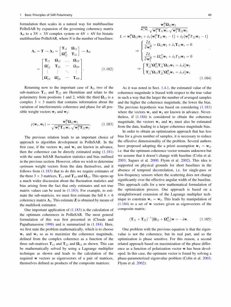
formulation then scales in a natural way for multibaselinePolInSAR by expansion of the governing coherency matrixΛN to a 3N � 3N complex system or 4N � 4N for bistaticmultibaseline PolInSAR, where N is the number of baselines:

Λ1 ¼ T ! Λ2 ¼T11 Ω12

ΩH12 T22

� �! ΛN

¼

T11 Ω12 . . . Ω1N

Ω�12 T22 ⋯ Ω2N

⋮ ⋮ ⋱ ⋮Ω�

1N Ω�2N ⋯ TNN

2666437775: ð1:182Þ

Returning now to the important case of Λ2, two of thesub-matrices T11 and T22 are Hermitian and relate to thepolarimetry from positions 1 and 2, while the third Ω12 is acomplex 3 � 3 matrix that contains information about thevariation of interferometric coherence and phase for all pos-sible weight vectors w1 and w2:

γ w1,w2ð Þ ¼ wH1 Ω12w2ffiffiffiffiffiffiffiffiffiffiffiffiffiffiffiffiffiffiffi

wH1 T11w1

p:ffiffiffiffiffiffiffiffiffiffiffiffiffiffiffiffiffiffiffiwH

2 T22w2

p : ð1:183Þ

The previous relation leads to an important choice ofapproach to algorithm development in PolInSAR. In thefirst case, if the vectors w1 and w2 are known in advance,then the coherence can be directly estimated using (1.181)with the same InSAR fluctuation statistics and bias outlinedin the previous section. However, often we wish to determineoptimum weight vectors from the data themselves, and itfollows from (1.183) that to do this we require estimates ofthe three 3 � 3 matrices, T11 and T22 and Ω12. This opens upa much wider discussion about the fluctuation statistics andbias arising from the fact that only estimates and not truematrix values can be used in (1.183). For example, to esti-mate the sub-matrices, we must first estimate the full 6 � 6coherency matrix Λ2. This estimate Z is obtained by means ofthe multilook estimator.

One important application of (1.183) is the calculation ofthe optimum coherences in PolInSAR. The most generalformulation of this was first presented in (Cloude andPapathanassiou 1998) and is summarized in (1.184). Here,we first state the problem mathematically, which is to choosew1 and w2 so as to maximize the coherence magnitude,defined from the complex coherence as a function of thethree sub-matrices T11 and T22 and Ω12 as shown. This canbe mathematically solved by using a Lagrange multipliertechnique as shown and leads to the calculation of therequired w vectors as eigenvectors of a pair of matrices,themselves defined as products of the composite matrices:

maxw1,w2

wH1 Ω12w2ffiffiffiffiffiffiffiffiffiffiffiffiffiffiffiffiffiffiffi

wH1 T11w1

p:ffiffiffiffiffiffiffiffiffiffiffiffiffiffiffiffiffiffiffiwH

2 T22w2

pL ¼ wH

1 Ω12w2 þ λ1 wH1 T11w1 � 1

� �þ λ2 wH2 T22w2 � 1

� �)

∂L∂wH

1

¼ Ω12w2 þ λ1T11w1 ¼ 0

∂L∂wH

2

¼ Ω�T12w1 þ λ2T22w2 ¼ 0

8>>><>>>:) T�1

22 ΩH12T

�111 Ω12w2 ¼ λ1λ

�2w2

T�111 Ω12T�1

22 ΩH12w1 ¼ λ1λ

�2w1

(:

ð1:184Þ

As it was noted in Sect. 1.4.1, the estimated value of thecoherence magnitude is biased with respect to the true valuein such a way that the larger the number of averaged samplesand the higher the coherence magnitude, the lower the bias.The previous hypothesis was based on considering (1.181)where the vectors w1 and w2 are known in advance. Never-theless, if (1.184) is considered to obtain the coherencemagnitude, the vectors w1 and w2 must also be estimatedfrom the data, leading to a larger coherence magnitude bias.

In order to obtain an optimization approach that has lessbias for a given number of samples, it is necessary to reducethe effective dimensionality of the problem. Several authorshave proposed adopting the a priori assumption w1 ¼ w2,i.e. that the optimum coherence vector remains unknown butwe assume that it doesn’t change with baseline (Colin et al.2003; Sagues et al. 2000; Flynn et al. 2002). This idea issupported on physical grounds for short baselines in theabsence of temporal decorrelation, i.e. for single-pass orlow-frequency sensors where the scattering does not changesignificantly over the effective angular width of the baseline.This approach calls for a new mathematical formulation ofthe optimization process. One approach is based on astraightforward extension of the Lagrange multiplier tech-nique to constrain w1 ¼ w2. This leads by manipulation of(1.184) to a set of w vectors given as eigenvectors of thecomposite matrix:

T11 þ T22ð Þ�1 Ω12 þΩH12

� �w ¼ �λw: ð1:185Þ

One problem with the previous equation is that the eigen-value is not the coherence, but its real part, and so theoptimization is phase sensitive. For this reason, a secondrelated approach based on maximization of the phase differ-ence as a function of polarization vector w has been devel-oped. In this case, the optimum vector is found by solving aphase-parameterized eigenvalue problem (Colin et al. 2003;Flynn et al. 2002):


ΩHw ¼ λTwΩH ¼ 1

2Ω12e

iϕ1 þΩH12e

�iϕ1� �

T ¼ 12

T11 þ T22ð Þ

8><>: :

ð1:186Þ

This has been shown to be equivalent to calculating thenumerical radius of the complex matrix A ¼ T�1/2Ω12T

�1/2.A proposed algorithm for finding this optimum state has beenpresented in (Colin et al. 2003; Colin et al. 2005). Onedrawback in this approach is that ϕ1 is a free parameter, andso either search or iterative methods must be used to securethe global optimum. This adds to the computational complex-ity for each pixel.

A third related approach has been proposed based on asub-space Monte Carlo searching algorithm (Sagues et al.2000). This limits the search for the optimum (again assum-ing w1 ¼ w2) to the diagonal elements of Ω12, i.e. toco-polarized or cross-polarized combinations across thewhole Poincaré sphere. This again acts to effectively limitthe dimensionality of the problem and demonstrates less biasthan the full Lagrange multiplier method. Finally, phasecentre super-resolution techniques based on the ESPRITalgorithm have also been proposed to find the optimumw vectors (Yamada et al. 2001).

In all these cases, a sub-optimum solution is obtainedcompared to the unconstrained Lagrange multiplier methodbut often with better numerical stability. Given the generalincreased processing overhead of employing optimization, itis always of interest to investigate the potential benefits ofemploying an optimization approach over simple linear, Pauliand circular options.

1.4.3 Model-Based Polarimetric SARInterferometry

The previous section considered an important optimisationproblem in PolInSAR, namely, to investigate the maximumvariation of coherence with polarization by solving an eigen-value problem. This section will be focused on some canoni-cal problems of interest in the remote sensing of land surfacesand try and use the mathematical solutions obtained to con-clude as to the potential of optimisation versus standardcoherence estimation in PolInSAR. We consider three impor-tant problems, scattering from non-vegetated surfaces, ran-dom volume scattering and finally a 2-layer surface+volumemixture which more closely matches the behaviour of naturalvegetated land surfaces.

1.4.3.1 PolInSAR for Bare Surface ScatteringThe starting point will be to consider the simplest case ofnon-vegetated terrain. Under the assumption of surface scat-tering only, the polarimetry can then be characterized as areflection symmetric random media with a coherency matrixT of the form shown in (1.187) (Cloude and Pottier 1996;Cloude et al. 2004). The interferometry, following range spec-tral filtering and assuming no temporal or SNR decorrelation,is characterized by a single parameter, i.e. the ground phase ϕ:

K¼ T�111 Ω12T�1

11 ΩH12 ¼ T�1

11 eiϕT11T�1

11 e�iϕT11 ¼

1 0 0

0 1 0

0 0 1

26643775 :

ð1:187Þ

From the previous equation, it follows that the optimumcoherences are obtained as eigenvectors of the matrix K asshown. By multiplying terms we see that the matrix K is justthe 3 � 3 identity matrix. This implies that all polarizationshave the same interferometric coherence and PolInSAR playsno role in surface scattering problems. This is not quite true inpractice for two important reasons: in practice there will bepolarization-dependent SNR decorrelation. In fact, recently ithas been suggested that such SNR coherence variations withpolarimetry be used for quantitative InSAR surface parameterestimation. This formulation assumes that the scattering fromthe surface occurs within a thin layer. If there is significantpenetration into the surface, then volume scattering effects canoccur and this will lead to volume decorrelation effects. Theseeffects have been observed for land ice (Treuhaft et al. 1996)and snow studies (Zebker and Villasenor 1992) where thesurface is non-vegetated but covered by a low-loss scatteringlayer. Nonetheless, (1.187) demonstrates how for bare surfacescattering PolInSAR plays only a secondary role. More inter-esting for application of natural land surfaces is to consider thepresence of volume scattering due to vegetation cover.

1.4.3.2 PolInSAR for Random Volume ScatteringWhen considering scattering from a volume, interest centres onthe special case of a random volume, i.e. one with macroscopicazimuthal symmetry (Cloude and Pottier 1996). In this case thepolarimetric coherency matrix T is diagonal. However, morecare is required over consideration of the interferometric phasein Ω12. In this case one must include the effects of volumedecorrelation due to the random vertical distribution of scatterers(Treuhaft et al. 1996). In this case, the interferometry mustinclude a complex integral I2 normalized by a real integral I1:


K ¼ T�111 Ω12T�1

11 ΩH12 ¼

I2I1

�� 21 0 0

0 1 0

0 0 1

26643775 ð1:188Þ

where

I1 ¼ e�2σhvcos θo

Zhv0

e2σz0cos θodz0 , I2

¼ e�2σhvcos θo

Zhv0

e2σz0cos θoeikzz0dz0 ð1:189Þ

where the vegetation is characterized by a height hv and meanextinction rate σ and θ0 represents the mean incidence angle.In (1.188), it is also observed that K is proportional to theidentity matrix, but this time the eigenvalues, all equal, aregiven by a ratio of integrals over the vertical distribution.This ratio is just the volume decorrelation displaying anincrease in phase variance and a vegetation bias to the groundphase determined by hv and σ:

γ wð Þ ¼ I2I1

¼ 2σ eiϕ zoð Þ

cos θo e2σ hv= cos θo � 1ð ÞZhv0

eikzz0e2σ z0cos θodz0

¼ pp1

ep1hv � 1ephv � 1

¼ γv

ð1:190Þ

where

p ¼ 2σcos θ0

,

p1 ¼ pþ ikz,

kz ¼ 4πΔθλ sin θ0

� 4πBn

λH tan θ0:

ð1:191Þ

Here the vertical interferometric wavenumber kz (Bamlerand Hartl 1998) appears as a function of the normal baselineBn, the wavelength λ as well as the sensor height H. Δθ is theangular separation of the baseline end points from the surfacepixel.

As it can be observed in (1.190), this coherence is inde-pendent of polarization, K has three degenerate eigenvaluesand PolInSAR plays no role in the analysis of random vol-ume scattering. This statement has to be modified in thepresence of oriented volumes (Treuhaft and Cloude 1999),i.e. ones with a preferred orientation of scattering elementssuch as that occurring in some agricultural crops and even inforestry applications at low frequencies. In such cases

PolInSAR does indeed play a role for volume scattering,with K developing three distinct eigenvalues. However, forthe treatment of forestry applications at L-band and above,such orientation effects are small and the random volumeassumption is justified (Papathanassiou et al. 2000).

In conclusion, both bare surfaces and random volumeslead to a degenerate eigenvalue spectrum for the matrix K.It is only when we combine these two effects together that wesee the potential benefits of employing PolInSAR processing.

1.4.3.3 PolInSAR Two-Layer Combined Surfaceand Random Volume Scattering

In the general case when combined surface and volumescattering occurs, then PolInSAR coherence optimisationbecomes useful as it is now demonstrated. In this two-layercase or Random-Volume-over-Ground (RVoG) modelapproach (Cloude and Papathanassiou 2003), the observedcoherence is given by a mixture formula:

γ wð Þ ¼ eiϕeγv þ μ wð Þ1þ μ wð Þ

¼ eiϕ γv þμ wð Þ

1þ μ wð Þ 1� γvð Þ� �

: ð1:192Þ

Here, the ground phase ϕ and complex volume coherenceγv are combined with a new real parameter μ, the ratio ofeffective surface, i.e. all scattering contributions with a phasecentre located at ϕ, to volume scattering. In effect, when μ¼ 0the scattering reduces to the case of random volume scattering,while when μ tends to infinity, it reduces to the surface scat-tering case. Interest centres on the intermediate case becauseone has an unknown, but constant, complex contribution fromthe volume scattering combined with a polarization-dependentsurface term. By isolating the polarization-dependent terms,the resulting coherence then lies along a straight line in thecomplex coherence plane as shown in (1.192).

This straight line model has been successfully tested onvaried forest data sets and seems to be a good fit for L- andP-band PolInSAR forestry applications. It is interesting to notehow the coherence varies as we adjust the single parameter μalong this line. Figure 1.15 illustrates three important cases. Inall three we first note how the coherence starts for small μ atsome value depending on the volume scattering contribution,0.8 in the example. It then initially decreases with increasingsurface contribution until reaching a turning point after which itincreases with μ, always approaching unity as μ tends to infinity.

In Fig. 1.15 three important special cases of the eigenvaluespectrum of K for this scenario are also superimposed. Thetop left shows the case when μ is always small, i.e. whenthere is strong volume scattering with high extinctionmasking the surface contributions. As polarization w isadjusted, then μ will also change, and the optimizer has anincentive to select the minimum μ channel to maximize coher-ence. At the other extreme, when μ is large and surface


scattering dominates, we see that the optimizer has an incen-tive instead to maximize μ in order to maximize coherence. Amore interesting case, and one that occurs often in practicefor L-band forestry applications, is the intermediate zonewhen the variation of μ (the μ spectrum) includes the turningpoint. In this case the coherence can be maximized by eitherincreasing or decreasing μ depending on circumstances.

Two important conclusions can be made from this. Firstly,in the mixed two-layer scattering case, the coherence varieswith polarization and so optimisation plays a role in PolInSARanalysis. Secondly, we see that we cannot simply associate themaximum coherence with, for example, the maximum valueof μ. Both maxima and minima of μ can lead to the optimumcoherence, depending on the circumstances. However, itfollows that if we can estimate the μ spectrum for any problem,then we can compare the max/min with the values for thestandard channel (linear, Pauli, etc.) to quantify the potentialbenefits of employing optimisation techniques.

The determination of the extreme points of the μ spectrumis related to a classical problem in radar polarimetry, namely,contrast optimisation (Novak and Burl 1990). The solution to

this is obtained as the eigenvalues of the product of the inversevolume times the surface polarimetric coherency matrices:

TV ¼ mI1

1 0 0

0 κ 0

0 0 κ

2666437775) T�1

v ¼ 1mI1

1 0 0

01κ

0

0 01κ

2666664

3777775

Ts ¼t11 t12 0

t�12 t22 0

0 0 t33

2666437775

) T�1v Ts ¼ 1

I1m

t11 t12 0

t�12κ

t22κ

0

0 0t33κ

266664377775

:

ð1:193Þ

0.65

-30 -20 -10 0mu (dB)

10 20 30 -30 -20 -10 0mu (dB)

10 20 30

-30 -20 -10 0mu (dB)

10 20 30

0.7

0.75

0.8

0.85 m3

m3

m2

m2

m1

m1

m3 m2 m1

Coh

eren

ce

0.9

0.95

1

0.65

0.7

0.75

0.8

0.85

Coh

eren

ce

0.9

0.95

1

0.65

0.7

0.75

0.8

0.85

Coh

eren

ce

0.9

0.95

1

Fig. 1.15 Variation of coherence with small (top left), large (top right) and intermediate (lower) μ values


Under the assumption of a random volume and reflectionsymmetric surface scattering component, the eigenvalues ofthis matrix can be determined analytically as

μ1 ¼ 12I1m

t11 þ t22κþ

ffiffiffiffiffiffiffiffiffiffiffiffiffiffiffiffiffiffiffiffiffiffiffiffiffiffiffiffiffiffiffiffiffiffiffiffiffiffiffiffiffiffit11 � t22

κ

� �2þ 4 t12j j2

κ

s0@ 1Aμ2 ¼ 1

2I1mt11 þ t22

κ�

ffiffiffiffiffiffiffiffiffiffiffiffiffiffiffiffiffiffiffiffiffiffiffiffiffiffiffiffiffiffiffiffiffiffiffiffiffiffiffiffiffiffit11 � t22

κ

� �2þ 4 t12j j2

κ

s0@ 1Aμ3 ¼ 1

I1mt33κ

� �

8>>>>>>>>>>>><>>>>>>>>>>>>:

)

γ1j jeiδ1 ¼ eiϕo γv þ μ1ð Þ1þ μ1



8>>>>>>><>>>>>>>:: ð1:194Þ

Equally importantly, the eigenvectors of this matrix indi-cate the w vectors that should be employed in PolInSAR tosecure these extreme coherence values. We note fromEq. (1.194) that the optimum contrast solutions are not gen-erally the simple HH, HV and VV channels. This supports theinvestigation of optimisation techniques based on fully polar-imetric data acquisition for PolInSAR processing.

1.5 Polarimetric SAR Tomography

3-D SAR Tomography (TomoSAR) is an experimentalmultibaseline (MB) interferometric mode achieving full 3-Dimaging in the range-azimuth-height space through elevationbeam forming, i.e. spatial (baseline) spectral estimation(Reigber and Moreira 2000). Thanks to TomoSAR, the reso-lution of multiple scatterers is made possible in height in thesame range-azimuth cell, overcoming a limitation of theconventional InSAR processing and complementingPolInSAR. TomoSAR can add more features for the analysisof complex scenarios, e.g. for the estimation of forest struc-ture and biomass, sub-canopy topography, soil humidity andice thickness monitoring and extraction of heights andreflectivities in layover urban areas. In order to retrieve infor-mation on the nature of the imaged scatterers, TomoSAR hasalso been extended to include the polarimetric information(briefly, PolTomoSAR) (Guillaso and Reigber 2005). Itjointly exploits multibaseline SAR data acquired with differ-ent polarization channels to improve the accuracy of theestimation of the vertical position of the imaged scatterersand to estimate a set of normalized complex coefficientscharacterizing the corresponding polarimetric scatteringmechanism.

The very first demonstration of the tomographic conceptwas carried out in 1995 by processing single-polarizationdata acquired in an anechoic chamber of a two-layer synthetictarget (Pasquali et al. 1995). TomoSAR was thenexperimented from an airborne platform a few years laterby acquiring L-band data by means of the DLR E-SARplatform over the Oberpfaffenhofen site (Reigber andMoreira 2000). Although this experiment was successful indemonstrating the 3-D imaging capabilities of forest volumesand man-made targets at L-band, two main limitations ofTomoSAR were apparent, namely, (i) the usually low num-ber of images available for processing to avoid large acquisi-tion times and the consequent temporal decorrelation and (ii)the difficulty of obtaining ideal uniformly spaced parallelflight tracks due to navigation/orbital considerations.

In order to mitigate the effects of acquisitionnon-idealities, most of the subsequent research on (single-polarization) TomoSAR investigated different imagingsolutions, model-based and not. Many experiments haveshown that the use of polarimetric information not onlyincrements the number of observables, but it also allows toenhance the accuracy of height estimation of scatterers, toincrease height resolution and to estimate a vector of complexcoefficients describing the scattering mechanism at eachheight (Guillaso and Reigber 2005). In forest scenarios, thecombination of multibaseline polarimetric data can be used toseparate ground and canopy scattering and to estimate theirvertical structures by following a relatively simple algebraicapproach (Tebaldini 2009).

1.5.1 TomoSAR and PolTomoSAR as SpectralEstimation Problems: Non-model-BasedAdaptive Solutions

As usual in SAR imaging and interferometry, after focusingon the range-azimuth plane, the K SAR images available forprocessing are assumed to be co-registered and properlycompensated for the flat-Earth phase. Moreover,N independent looks (here multiple adjacent pixels) areused for processing. For each n-th look, the complexamplitudes of the pixels observed in the K SAR images atthe same range-azimuth coordinate are collected in the K � 1complex-valued vector y(n) (Lombardini and Reigber 2003).y(n) is characterized by its covariance matrix. It can bedemonstrated that the generic (l, m)-th element of R can bewritten as

R½ �l,m ¼Z

F zð Þ exp j kz,l � kz,mð Þzf gdz ð1:195Þ

where F(z) is the unknown vertical distribution of thebackscattered power as a function of the height z and kz, mis the vertical wavenumber at the m-th track. From (1.195), it


is apparent the Fourier relationship existing between the MBcovariances and the profile of the backscattered power, and itjustifies the use of spectral estimation as a processing tool toestimate F(z).

The inversion of (1.195) for the estimation of F(z) cannotbe carried out through a plain Fourier-based 3-D focusing asit suffers from inflated sidelobes and poor height resolution.Among the investigated alternatives, a state-of-the-art solu-tion is the adaptive beam forming (shortly, ABF), which isbased on the Capon spectral estimator, and it has beendemonstrated to have remarkable sidelobe rejection and res-olution capabilities.

The single-polarization ABF spectral estimation problemcan be equivalently stated as the problem of designing acomplex-valued finite impulse response filter h of orderK that leaves undistorted the multibaseline signal componentat the height under test, say z, while rejecting possible othercomponents from noise and other heights (Lombardini andReigber 2003). In formulas

minh

hT�bRh subjectto hT�a zð Þ ¼ 1 ð1:196Þ

where a(z) is the so-called steering vector, with genericelement [a(z)]k ¼ exp { jkz, kz } for k ¼ 1, . . ., K, and bR isthe sample covariance estimate. Notice that the resultingABF filter h depends on bR, and it varies with z; In particular,the dependency on bR results in a null-placing at properheights in the filtering operation, thus increasing resolutionand sidelobe suppression in the final estimate of F(z). Thesolution to the optimization problem (1.196) can be found inclosed-form (Lombardini and Reigber 2003).

If fully polarimetric data are available, without losinggenerality, they can be combined in the Pauli basis. Theresulting MB data vectors y1(n), y2(n) and y3(n) can then bestacked one on top of the other in order to form the 3K-dimensional multibaseline-polarimetric data vector yP(n).As a consequence, a MB-polarimetric sample covariancematrix bRP can be calculated from yP(n). Different from thesingle polarimetric case, the profile has now to be estimatedalso by considering the polarization state at the targetedheight. In this sense, the definition of the steering vectorcan be extended to the polarimetric case by means of athree-dimensional target vector w whose elements arecomplex-valued coefficients describing the scattering mech-anism in the Pauli basis, with k w k2 ¼ 1. In formulas, thepolarimetric steering vector b(z, w) is given by

b z,wð Þ ¼ B zð Þw, ð1:197Þ

where

B zð Þ=a zð Þ 0 0

0 a zð Þ 0

0 0 a zð Þ

264375 : ð1:198Þ

The ABF optimization problem (1.196) can be extendedto the MB-polarimetric case as follows (Sauer et al. 2011):

minhP

hT�P bRPhP subjectto hT�P b z,wð Þ ¼ 1 ð1:199Þ

where hP is the multibaseline-polarimetric ABF filterresponse. Now, hP is optimized in order to place propernulls in height and in the polarimetric space generated byw. Notice that the dependence of w on z has been formallydropped for easiness of notation. From (1.199), the power ofthe filtered signal is

bFABF z,wð Þ ¼ 1

bT� z,wð ÞbRPb z,wð Þð1:200Þ

which is still a function of w. To estimate the vertical powerdistribution as a function of the only z, and the correspondingw, one can maximize (1.200) over w to finally obtain

bFABF zð Þ ¼ 1

λmin BT� zð Þ bR�1

P B zð Þn o ð1:201Þ

where λmin{�} denotes the minimum eigenvalue operator. Theresulting bwABF zð Þ is the eigenvector associated with λmin. It isworth noting that the multibaseline-polarimetric ABF estima-tor (1.201) enhances the discrimination of particularscatterers or features. In other words, it is able to extract arank 1 polarimetric information. This is generally the case ofman-made targets like buildings in urban scenarios.

However, it can happen that the scatterers present at agiven z are characterized by a random polarimetricbehaviour, and they are more properly described by a 3 � 3polarimetric covariance matrix T(z) rather than by a deter-ministic target vector (Ferro-Famil et al. 2012). This is gen-erally the case in natural scenarios like forests. In this way, ascattering mechanism at the generic z will contribute to RP

with T(z)N

[a(z)aT�(z)]. In light of this, the polarimetricABF estimator from the rank 1 formulation (1.201) can beextended in a full-rank sense (Ferro-Famil et al. 2012). Thederivation of such estimate is based on the definition of a full-rank objective function which uses the polarimetric spaninstead of the intensity associated with a given scatteringmechanism. The full-rank ABF estimator then is


bFABF�FR zð Þ ¼ trace BT� zð Þ bR�1

P B zð Þh i�1� �

, ð1:202Þ

bTABF zð Þ ¼ BT� zð ÞbR�1

P B zð Þh i�1

: ð1:203Þ

The availability of the polarimetric coherence matrixmakes possible the full exploitation of the polarimetric infor-mation for the characterization of the scattering, allowing the3-D calculation of parameters like, e.g. entropy and degree ofpolarization, as well as the application of polarimetricdecompositions.

1.5.2 Model-Based PolTomoSAR

As mentioned in Sect. 1.6.1, the non-model-based ABF pos-sess some intrinsic degree of super-resolution, i.e. it is able toseparate scatterers with a height difference lower than theRayleigh resolution limit, which in turn depends on themaximum available track separation. However, a highersuper-resolution could be needed in some applications. Forthis reason, a solution is to resort to model-based tomo-graphic processors, which generally exploit the statisticaldescription of the received signal or equivalently of thescattering behaviours present in the observed scene.

Several methods have been proposed for single-polarization and then extended to full-polarization MB datasets. For instance, the MUSIC (multiple signal classification)is matched to point-like targets (Frey and Meier 2011), and itexploits the fact that the multibaseline response of each point-like scatterer (i.e. the steering vector) in the backscatteredradiation is orthogonal to the noise subspace. As a conse-quence, closed-form solution of the MUSIC PolTomoSARfunctional can be found that outputs the scattering mecha-nism of each scatterer (Sauer et al. 2011). Still in the categoryof the eigen-based processors, the weighted signal subspacefitting can cope with more complex statistical descriptions ofdistributed and coherent scatterers, although a multidimen-sional optimization is required (Huang et al. 2011).

Alternatively to the eigen-based PolTomoSAR, a solutionadaptive to both coherent and distributed scatterers, but pos-sibly leading to a lower computational time, is the so-calledcovariance matching estimator (COMET). If themultibaseline data are jointly Gaussian distributed, theknowledge of the MB-multipolarimetric covariance matrixRP is enough to perform a maximum likelihood(ML) estimation of the parameters describing the verticaldistribution of the backscattered power. It can bedemonstrated that the global ML problem can bedecomposed by means of the extended invariance principleinto a cascade of two ML problems (i.e. the estimation of RP

and the estimation of the parameters of interest from bRP ),leading to an asymptotically equivalent solution and with a

non-negligible reduction of the computational complexity.Under the Gaussian hypothesis, the resulting COMETestimates can be obtained from the following minimizationproblem (Tebaldini and Rocca 2010):

bρ ¼ argminρ

trace bR�1

P RP ρð Þ � bRP

h ibR�1

P RP ρð Þ � bRP

h i� �ð1:204Þ

where ρ is the vector containing the parameters that describethe multibaseline covariances. Equation (1.204) can be seenas the weighted Frobenius norm of the approximation error

RP ρð Þ � bRP with weight bR�1

P . Worth of notice, the COMETestimator can be used also when data are not Gaussian,although it is not asymptotically optimal anymore.

1.5.3 Coherence Tomography

Besides the development of spectral estimation- and model-based PolTomoSAR, also the so-called (polarimetric) coher-ence tomography methods have been proposed which recon-struct the vertical distribution of scatterers from complexcoherence measurements of volumetric scatterers. In a fewwords, the structure function is approximated through aweighted sum of a series of basis functions (Cloude 2007b).The individual parameterization has then to be inverted usinga (limited) number of interferometric measurements at thesame or different polarizations. In this class of “hybrid”algorithms, the different polarization channels can be used,e.g. to find a polarization state with lowest groundcontribution.

References

Alonso Gonzalez A, Lopez Martinez C, Salembier P (2012) Filteringand segmentation of polarimetric SAR data based on binary partitiontrees. IEEE Trans Geosci Remote Sens 50:593–605

Arii M, Van Zyl JJ, Kim Y (2011) Adaptive model-based decompositionof polarimetric SAR covariance matrices. IEEE Trans GeosciRemote Sens 49:1104–1113

Balanis CA (1989) Advanced engineering electromagnetics. Wiley,New York

Ballester Berman JD, Lopez Sanchez JM, Fortuny Guasch J (2005)Retrieval of biophysical parameters of agricultural crops using polar-imetric SAR interferometry. IEEE Trans Geosci Remote Sens43:683–694

Bamler R, Hartl P (1998) Synthetic aperture radar interferometry. InvProb 14:R1–R54

Bebbington DHO (1992) Target vectors – spinorial concepts. In: ProcSecond International Workshop on Radar Polarimetry

Beckmann P, Spizzichino A (1987) The scattering of electromagneticwaves from rough surfaces. Artech House, Norwood

Boerner WM et al (1998) Polarimetry in radar remote sensing: basic andapplied concepts. In: Ryerson RA (ed) Manual of remote sensing:principles and applications of imaging radar, vol 3. Wiley, Hoboken,pp 271–356


Cameron WL, Leung LK (1990) Feature motivated polarization scatter-ing matrix decomposition. In: Proceedings of IEEE 1990 Interna-tional Radar Conference

Chandrasekhar S (1960) Radiative transfer. Dover, New YorkCloude SR (1988) Uniqueness of target decomposition theorems in

radar polarimetry. In: Proceedings of NATO Adv. Res. Workshopon Direct Inverse Methods in Radar Polarimetry

Cloude SR (2007a) The dual polarization H/alpha decomposition: aPALSAR case study. Paper presented at 2007 international work-shop on science and applications of SAR polarimetry and Polarimet-ric interferometry (POLinSAR)

Cloude SR (2007b) Dual-baseline coherence tomography. IEEE GeosciRemote Sens Lett 4:127–131

Cloude SR, Papathanassiou KP (1998) Polarimetric SAR interferome-try. IEEE Trans Geosci Remote Sens 36:1551–1565

Cloude SR, Papathanassiou KP (2003) A 3-stage inversion process forpolarimetric SAR interferometry. IEE Proc Radar Sonar Navigation150:125–134

Cloude SR, Pottier E (1996) A review of target decomposition theoremsin radar polarimetry. IEEE Trans Geosci Remote Sens 34:498–518

Cloude SR, Corr DG, Williams ML (2004) Target detection beneathfoliage using polarimetric SAR interferometry. Waves RandomMedia 14:393–414

Colin E, Titin Schneider C, Tabbara W (2003) Investigation of differentinterferometric coherence optimisation methods. Paper presented at2003 International Workshop on Science and Applications of SARPolarimetry and Polarimetric Interferometry (POLinSAR)

Colin E, Titin Schneider C, Tabbara W (2005) Coherence optimizationmethods for scattering centre separation in polarimetric interferome-try. J Electrom Waves App 19:1237–1250

Curlander JC, McDonough RN (1991) Synthetic aperture radar: systemsand signal processing. John Wiley & Sons, New York

Dall J, Papathanassiou KP, Skriver H (2003) Polarimetric SAR interfer-ometry applied to land ice: first results. In: Proceedings of IEEE2003 International Geoscience and Remote Sensing Symposium(IGARSS)

De Grandi G, Lee JS, Schuler D, Nezry E (2003) Texture and specklestatistics in polarimetric SAR synthesized images. IEEE TransGeosci Remote Sens 41:2070–2088

Deledalle CA, Tupin F, Denis L (2010) Polarimetric SAR estimationbased on non-local means. In: Proceedings of IEEE 2010International Geoscience and Remote Sensing Symposium(IGARSS)

Doob JL, Ornstein LS, Uhlenbeck GE, Rice SO, Kac M,Chandrasekhar S, Wax N (1954) Selected papers on noise andstochastic processes. Dover Publications, Mineola/New York

Ferro-Famil L, Huang Y, Reigber A (2012) High-resolution SARtomography using full-rank polarimetric spectral estimators. In:Proceedings of IEEE 2012 International Geoscience and RemoteSensing Symposium (IGARSS)

Flynn T, Tabb M, Carande R (2002) Coherence region shape estimationfor vegetation parameter estimation in POLINSAR. In: Proceedingsof IEEE 2002 International Geoscience and Remote Sensing Sym-posium (IGARSS)

Foucher S, Landry T, Lopez Martinez C, Charbonneau F, Gagnon L(2012) An evaluation of PolSAR speckle filters on compact-polimages. In: Proceedings of IEEE 2012 International Geoscienceand Remote Sensing Symposium (IGARSS)

Freeman A, Durden SL (1998) A three-component scattering model forpolarimetric SAR data. IEEE Trans Geosci Remote Sens36:963–973

Frey O, Meier E (2011) Analyzing tomographic SAR data of a forestwith respect to frequency, polarization, and focusing technique.IEEE Trans Geosci Remote Sens 49:3648–3659

Gabriel AK, Goldstein RM, Zebker HA (1989) Mapping small elevationchanges over large areas: differential radar interferometry. J Geo Res94:9183–9191

Goodman JW (1976) Some fundamental properties of speckle. J OptSoc Am 66:1145–1149

Goodman JW (1985) Statistical optics. John Wiley & Sons, New YorkGuillaso S, Reigber A (2005) Scatterer characterisation using polarimet-

ric SAR tomography. In: Proceedings of IEEE 2005 InternationalGeoscience and Remote Sensing Symposium (IGARSS)

Hajnsek I, Pottier E, Cloude SR (2003) Inversion of surface parametersfrom polarimetric SAR. IEEE Trans Geosci Remote Sens41:727–744

Hoekman DH, Quinones MJ (2002) Biophysical forest type characteri-zation in the colombian amazon by airborne polarimetric SAR. IEEETrans Geosci Remote Sens 40:1288–1300

Huang Y, Ferro-Famil L, Reigber A (2011) Under-foliage object imag-ing using SAR tomography and polarimetric spectral estimators.IEEE Trans Geosci Remote Sens 50:2213–2225

Huynen JR (1970) Phenomenological theory of radar targets. Ph.D.thesis, Technical University of Delft, The Netherlands

IEEE standard number 145 (1983) IEEE standard definitions of termsfor antennas

Jones RC (1941a) A new calculus for the treatment of optical systems. IDescrip Discussion J Opt Soc Am 31:488–493

Jones RC (1941b) A new calculus for the treatment of optical systems. IIProof of the three general equivalence theorems. J Opt Soc Am31:493–499

Jones RC (1941c) A new calculus for the treatment of optical systems.III: The Stokes theory of optical activity. J Opt Soc Am 31:500–503

Kasilingam D, Schuler D, Lee JS, Malhotra S (2002) Modulation ofpolarimetric coherence by ocean features. In: Proceedings of IEEE2002 International Geoscience and Remote Sensing Symposium(IGARSS)

Kay SM (1993) Fundamentals of statistical signal processing. Estima-tion theory. Prentice-Hall, Englewood Cliffs

Kennaugh K (1951) Effects of type of polarization on echocharacteristics, Technical report. Ohio State University

Kong JA (ed) (1990) Polarimetric remote sensing. Elsevier, New YorkKrogager E (1990) New decomposition of the radar target scattering

matrix. Electron Lett 26:1525–1527Lee JS (1981) Speckle analysis and smoothing of synthetic aperture

radar images. Comp Graphics Im Proc 17:24–32Lee JS, Grunes MR, Mango SA (1991) Speckle reduction in

multipolarization, multifrequency SAR imagery. IEEE Trans GeosciRemote Sens 29:535–544

Lee JS, Hoppel KW, Mango SA, Miller AR (1994) Intensity and phasestatistics of multilook polarimetric and interferometric SAR imagery.IEEE Trans Geosci Remote Sens 32:1017–1028

Lee JS, Grunes MR, De Grandi G (1999) Polarimetric SAR specklefiltering and its implication for classification. IEEE Trans GeosciRemote Sens 37:2363–2373

Lee JS, Schuler DL, Ainsworth TL, Krogager E, Kasilingam D, BoernerWM (2002) On the estimation of radar polarization orientation shiftsinduced by terrain slopes. IEEE Trans Geosci Remote Sens40:30–41

Lee JS, Cloude SR, Papathanassiou KP, Grunes MR, Woodhouse IH(2003) Speckle filtering and coherence estimation of PolInSAR datafor forest applications. IEEE Trans Geosci Remote Sens41:2254–2263

Lee JS, Grunes MR, Schuler DL, Pottier E, Ferro-Famil L (2006)Scattering-model-based speckle filtering of polarimetric SAR data.IEEE Trans Geosci Remote Sens 44:176–187

Lombardini F, Reigber A (2003) Adaptive spectral estimators formultibaseline SAR tomography with airborne L-band data. In:Proceedings of IEEE 2003 International Geoscience and RemoteSensing Symposium (IGARSS)

Lopes A, Touzi R, Nezry E (1990) Adaptive speckle filters and sceneheterogeneity. IEEE Trans Geosci Remote Sens 28:992–1000

Lopez Martínez C, Fabregas X (2003) Polarimetric SAR speckle noisemodel. IEEE Trans Geosci Remote Sens 41:2232–2242


Lopez Martínez C, Fabregas X (2008) Model-based polarimetric SARspeckle filter. IEEE Trans Geosci Remote Sens 46:3894–3907

Luneburg E (2002) Aspects of radar polarimetry. Elektrik- Turkish JElectr Eng Comput Sci 10:219–243

Mattia F, le Toan T, Lee JS, Schuler DL (2003) On the sensitivity ofpolarimetric coherence to small and large scale surface roughness.In: Proceedings of IEEE 2003 International Geoscience and RemoteSensing Symposium (IGARSS)

McCrea WH, Whipple FJW (1940) Random paths in two and threedimensions. Proc R Soc Edinburgh 60:281–298

Mette T, Papathanassiou KP, Hajnsek I (2004) Biomass estimation fromPolInSAR over heterogeneous terrain. In: Proc IEEE 2004 Interna-tional Geoscience and Remote Sensing Symposium (IGARSS)

Morio J, Refregier P, Goudail F, Dubois Fernandez P, Dupuis X (2007)Application of information theory measures to polarimetric andinterferometric SAR images. In: Proceedings of 2007 InternationalConference on Physics in Signal and Image Processing

Novak L, Burl MC (1990) Optimal speckle reduction in polarimetricSAR imagery. IEEE Trans Aerosp Electron Syst AES-26:293–305

Oliver C, Quegan S (1998) Understanding synthetic aperture radarimages. Artech House, Boston

Paladini R, Ferro-Famil L, Pottier E, Martorella M, Berizzi F, DalleMese E (2012) Lossless and sufficient-invariant decomposition ofrandom reciprocal target. IEEE Trans Geosci Remote Sens50:3487–3501

Papathanassiou KP, Cloude SR (2001) Single baseline polarimetricSAR interferometry. IEEE Trans Geosci Remote Sens39:2352–2363

Papathanassiou KP, Cloude SR, Reigber A (2000) Single and multi-baseline polarimetric SAR interferometry over forested terrain. In:Proceedings of 2000 European Conference on Synthetic ApertureRadar (EUSAR)

Papathanassiou KP, Cloude SR, Liseno A, Mette T, Pretzsch H (2005a)Forest height estimation by means of polarimetric SAR interferome-try: actual status and perspectives. Paper presented at 2005 Interna-tional Workshop on Science and Applications of SAR Polarimetryand Polarimetric Interferometry (POLinSAR)

Papathanassiou KP, Hajnsek I, Nagler T, Rott H (2005b) PolarimetricSAR interferometry for snow cover parameter estimation. Paperpresented at 2005 international workshop on science andapplications of SAR polarimetry and polarimetric interferometry(POLinSAR)

Papoulis A (1984) Probability, random variables and stochastic pro-cesses. McGraw-Hill, New York

Pasquali P, Prati C, Rocca C, Seymour M, Fortuny J, Olmer E, Sieber AJ(1995) A 3D SAR experiment with EMSL data. In: Proceedings ofIEEE 1995 International Geoscience and Remote Sensing Sympo-sium (IGARSS)

Raney RK (1983) Transfer function for partially coherent SAR systems.IEEE Trans Aerosp Electron Syst AES-19:740–750

Reigber A, Moreira A (2000) First demonstration of airborne SARtomography using multibaseline L-band data. IEEE Trans GeosciRemote Sens 38:2142–2152

Reigber A, Papathanassiou KP, Cloude SR, Moreira A (2000) SARtomography and interferometry for the remote sensing of forestedterrain. In: Proceedings of 2000 European Conference on SyntheticAperture Radar (EUSAR)

Sagues L, Lopez Sanchez JM, Fortuny J, Fabregas X, Broquetas A,Sieber AJ (2000) Indoor experiments on polarimetric SAR interfer-ometry. IEEE Trans Geosci Remote Sens 38:671–684

Sarabandi K (1997) Δk-radar equivalent of interferometric SAR’s: atheoretical study for determination of vegetation height. IEEE TransGeosci Remote Sens 35:1267–1276

Sauer S, Ferro-Famil L, Reigber A, Pottier E (2011) Three-dimensionalimaging and scattering mechanism estimation over urban scenesusing dual-baseline polarimetric InSAR observations at L-band.IEEE Trans Geosci Remote Sens 49:4616–4629

Schleher DC (1975) Radar detection in log normal clutter. In:Proceedings of IEEE 1975 International Radar Conference

Schneider Zandona R, Papathanassiou K, Hajnsek I, Moreira A (2005)Polarimetric interferometry over urban areas: information extractionusing coherent scatterers. In: Proc IEEE 2005 International Geosci-ence and Remote Sensing Symposium (IGARSS)

Stokes GG (1852) On the composition and resolution of streams ofpolarized light from different sources. Trans Cambridge Phil Soc9:399–416

Tabb M, Carande R (2001) Robust inversion of vegetation structureparameters from low frequency polarimetric interferometric SAR.In: Proceedings of IEEE 2001 International Geoscience and RemoteSensing Symposium (IGARSS)

Tebaldini S (2009) Algebraic synthesis of forest scenarios frommultibaseline PolInSAR data. IEEE Trans Geosci Remote Sens47:4132–4142

Tebaldini S, Rocca F (2010) Single and multipolarimetric SAR tomog-raphy of forested areas: a parametric approach. IEEE Trans GeosciRemote Sens 48:2375–2387

Tough RJA, Blacknell D, Quegan S (1995) A statistical description ofpolarimetric and interferometric synthetic aperture radar data. Proc RSoc London 449:567–589

Touzi R (2007) Target scattering decomposition in terms of roll-invariant target parameters. IEEE Trans Geosci Remote Sens45:73–84

Touzi R, Lopes A (1994) The principle of speckle filtering in polarimet-ric SAR imagery. IEEE Trans Geosci Remote Sens 32:1110–1114

Touzi R, Lopes A, Bruniquel J, Vachon PW (1999) Coherence estima-tion for SAR imagery. IEEE Trans Geosci Remote Sens 37:135–149

Touzi R, Boerner WM, Lee JS, Luneberg E (2004) A review of polar-imetry in the context of synthetic aperture radar: concepts andinformation extraction. Can J Remote Sens 30:380–407

Touzi R, Deschamps A, Rother G (2007) Wetland characterization usingpolarimetric RADARSAT-2 capability. Can J Remote Sens33:56–67

Treuhaft RN, Cloude SR (1999) The structure of oriented vegetationfrom polarimetric interferometry. IEEE Trans Geosci Remote Sens37:2620–2624

Treuhaft RN, Madsen S, Moghaddam M, Van Zyl JJ (1996) Vegetationcharacteristics and underlying topography from interferometric data.Radio Sci 31:1449–1495

Trunk GV (1972) Radar properties of non-Rayleigh sea echo. IEEETrans Aerosp Electron Syst AES-8:196–204

Trunk GV, George SF (1970) Detection of targets in non-gaussian seaclutter. IEEE Trans Aerosp Electron Syst AES-6:620–628

Ulaby FT, Elachi C (1990) Radar polarimetry for geoscienceapplications. Artech House, Norwood

Ulaby FT, Moore RK, Fung AK (1986a) Microwave remote sensing:active and passive, vol III. Artech House, Norwood

Ulaby FT, Moore RK, Fung AK (1986b) Microwave remote sensing:active and passive, vol II. Artech House, Norwood

Van Zyl JJ, Arii M, Kim Y (2011) Model-based decomposition ofpolarimetric SAR covariance matrices constrained for nonnegativeeigenvalues. IEEE Trans Geosci Remote Sens 49:3452–3459

Vasile G, Trouve E, Lee JS, Buzuloiu V (2006) Intensity-driven adap-tive-neighbourhood technique for polarimetric and interferometricSAR parameters estimation. IEEE Trans Geosci Remote Sens44:1609–1621

Wakabayashi H, Matsuoka T, Nakamura K, Nishio F (2004) Polarimet-ric characteristics of sea ice in the sea of Okhotsk observed byairborne L-band SAR. IEEE Trans Geosci Remote Sens42:2412–2425

Wiener N (1930) Generalized harmonic analysis. Acta Mathematica5:118–258

Williams ML (1999) Prediction and observation of SAR clutter fromvegetation canopies. In: Proc IEEE 1999 International Geoscienceand Remote Sensing Symposium (IGARSS)


Williams ML, Cloude SR (2005) Predictions of SAR polarimetryand InSAR coherence for a model wheat canopy. In: Proceedingsof IEEE 2005 International Geoscience and Remote SensingSymposium (IGARSS)

Yamada H, Yamaguchi Y, Rodriguez E, Kim Y, Boerner WM (2001)Polarimetric SAR interferometry for forest canopy analysis by usingthe super-resolution method. IEICE Trans Electron E84-C:1917–1924

Yamaguchi Y, Moriyama T, Ishido M, Yamada H (2005) Four-component scattering model for polarimetric SAR image decompo-sition. IEEE Trans Geosci Remote Sens 43:1699–1706

Zebker HA, Villasenor J (1992) Decorrelation in interferometric radarechoes. IEEE Trans Geosci Remote Sens 30:950–959

Open Access This chapter is licensed under the terms of the Creative Commons Attribution 4.0 International License (http://creativecommons.org/licenses/by/4.0/), which permits use, sharing, adaptation, distribution and reproduction in any medium or format, as long as you give appropriatecredit to the original author(s) and the source, provide a link to the Creative Commons license and indicate if changes were made.

The images or other third party material in this chapter are included in the chapter’s Creative Commons license, unless indicated otherwise in acredit line to the material. If material is not included in the chapter’s Creative Commons license and your intended use is not permitted by statutoryregulation or exceeds the permitted use, you will need to obtain permission directly from the copyright holder.


Documents

Basic Principles of SAR Polarimetry 1