BAR-ILAN UNIVERSITY

High-Resolution Double-Pulse-Pair Brillouin

Optical Correlation-Domain Analysis

OREL SHLOMI

Submitted in partial fulfillment of the requirements for the Master's

Degree in the Faculty of Engineering, Bar-Ilan University

Ramat-Gan, Israel 2016

This work was carried out under the supervision of Prof. Avi

Zadok, Faculty of Engineering, Bar-Ilan University

Acknowledgments B"H

“Showing gratitude is one of the simplest yet most powerful things humans can do for

each other.” ― Randy Pausch, The Last Lecture

I would like to dedicate these next few lines to thank those who have assisted,

guided and encouraged me throughout these two years to complete this research.

First and foremost I would like to thank the G-d, without whom nothing could be

carried out.

When I first started working under the guidance of Prof. Avi Zadok I did not really

know what my future holds. Already during my first degree I began working on my final

undergraduate project in the group. In retrospect, although that project did not approach

the size of a research thesis, it nevertheless laid the foundations for my research work. Even

at that stage, I already realized that I chose the advisor that is best for me.

I would like to thank Prof. Avi Zadok for taking me under his wing to be part of his

research group. His unique dedication and devotion to his group members and to the

product of their research was bestowed onto me and is extremely appreciated. He requires

a high level of research and writing standards, and for that and more I am extremely

grateful.

Thanks to Yosef London, who gave me the "baptism of fire" as my undergraduate

project advisor. He provided me with the tools needed to challenge myself, so that I could

think of new research methods and of improvements to existing ones.

Thanks go also to Eyal Preter (soon to be Dr.), who was my lab partner, and helped

me build the setup that served us both; to Dr. Yair Antman and Yoni Stern, who previously

worked on fiber sensing projects in our group and helped me along the way.

I would also like to mention all my other colleagues from Dr. Avi Zadok’s group, past

and present, for their valuable contribution and for sharing their experience and knowledge:

Dr. Arkady Rudnitsky, Dr. Ran Califa, Dr. Shahar Levi, Nadav Arbel, Dvir Munk, Assaf Ben

Amram, Hagai Diamandi, Moshe Kathman, Dr. Mirit Chen and Gil Bashan. I would also like to

mention Niv Arad, who was my undergraduate project partner at the beginning of this

expedition. Thanks also to Dr. Dexin Ba, who came from faraway China to conduct post-

doctoral research with our group, and contributed from his broad knowledge to all team

members in general, and to me in particular.

I would like to thank the administrative team of the Engineering Faculty of Bar-Ilan

University, especially Mrs. Dina Yemini, for her support in any subject needed, and also to

Mrs. Adi Hevroni which helped a lot during the last two years.

Obviously, I thank my incredible family. My parents, Elazar and Kineret Shlomi, for

supporting me and for giving me a nice and warm home to live in, to my two sisters and my

younger brother: Ortal, Shiran and Elroyi, with whom I always love to be. And finally, to my

fiancé Hodaya, for her quiet patience and unwavering love were there for me.

Table of Contents

Acknowledgments

LIST OF FIGURES

Acronyms

Notations

List of Publications

Abstract ........................................................................................................................i

1. Introduction ............................................................................................................. 1

1.1 Optical fibers sensors ........................................................................................... 1

1.2 Rayleigh scattering-based sensors.......................................................................... 2

1.3 Raman Scattering-based sensors ........................................................................... 4

1.4 Stimulated Brillouin scattering (SBS) ...................................................................... 5

1.4.1 Mathematical analysis of stimulated Brillouin scattering .................................... 8

1.5 Sensing based on stimulated Brillouin scattering ................................................... 17

1.6 Implementation schemes of distributed Brillouin sensors ....................................... 18

1.6.1 Brillouin optical time domain analysis (B-OTDA) .............................................. 18

1.6.2 Differential double pulse pair measurements .................................................. 23

1.6.3 Brillouin optical correlation domain analysis ................................................... 26

1.6.4 Phase-coded Brillouin optical correlation domain analysis ................................ 28

1.6.5 Hybrid B-OTDA / B-OCDA method .................................................................. 32

1.7 Research objectives ........................................................................................... 35

2. Principle of operation, analysis and simulations .......................................................... 37

2.1 Rationale and principle of operation .................................................................... 37

2.2 Simulations results ............................................................................................. 38

2.3 Signal to noise ratio ............................................................................................ 45

2.3.1 Noise mechanisms ....................................................................................... 45

3. Experiments and results ........................................................................................... 51

3.1 Setup and main components ............................................................................... 51

3.1.1 Polarization control ...................................................................................... 56

3.1.2 Scanning of correlation peaks positions .......................................................... 57

3.2 Results .............................................................................................................. 59

4. Summary and discussion .......................................................................................... 64

4.1 Comparison with other Brillouin sensing protocols ................................................ 64

4.2 Limitations ........................................................................................................ 66

4.3 Future work ...................................................................................................... 67

5. Bibliography ........................................................................................................... 69

א ......................................................................................................................... תקציר

LIST OF FIGURES

Figure 1. Schematic illustration of underlying mechanisms and positive feedback in

stimualted Brillouin scattering (SBS). ............................................................................... 7

Figure 2. Illustration of the SBS gain spectrum. ................................................................. 7

Figure 3. Illustration of the three scattering effects: Rayleigh scattering, stimulated Raman

scattering, and SBS........................................................................................................ 8

Figure 4. An illustration of the SBS interaction between a pulsed pump and a counter-

propagating, continuous signal. .................................................................................... 19

Figure 5. A normalized local Brillouin gain spectrum, as measured by Brillouin optical time-

domain analysis (B-OTDA). ........................................................................................... 21

Figure 6. Experimental setup of long range B-OTDA ........................................................ 22

Figure 7. The measured Brillouin frequency shift as a function of position along 325 km of

fiber, and evolution of the Brillouin gain. ....................................................................... 22

Figure 8. Measured SBS gain map as a function of position and of frequency detuning

between pump and signal, and magnified view of the gain map around a 5 cm fiber section.

................................................................................................................................. 23

Figure 9. Illustration of double pulse pair (DPP) B-OTDA traces of the Brillouin signal in the

beginning of a fiber under test, and their differential signal. ............................................ 24

Figure 10. Measured DPP B-OTDA signal traces at the output of a 2 km long fiber, and the

difference between the two traces. .............................................................................. 25

Figure 11. Measured Brillouin gain spectra and Brillouin frequency shift as a function of

position, towards the end of a 2 km long fiber using a DPP B-OTDA setup. A segment of 2 cm-

long fiber, which heated to 76 °C, is identified in the measurements. ............................... 25

Figure 12. Illustration of spatial confinement of SBS in Brillouin optical correlation domain

analysis (B-OCDA). ...................................................................................................... 27

Figure 13. Results of ultra-high resolution B-OCDA.......................................................... 27

Figure 14. Illustration of counter-propagating, binary phase-coded pump and signal waves

and their inner product. The two waves are correlated at the center only. ........................ 29

Figure 15. B-OCDA gain mapping of a 40-meter-long fiber and a 200-meters-long fiber. ..... 30

Figure 16. Simulated acoustic field magnitude in B-OCDA, with phase modulation by a

random sequence and a with a perfect Golomb code. ..................................................... 32

Figure 17. Illustration of phase-coded B-OCDA, with an overlaying pump pulse ................. 33

Figure 18. Simulated magnitude of the acoustic wave density in B-OCDA with an overlaying

pump pulse. ............................................................................................................... 34

Figure 19. Simulated output signal power as a function of time, in B-OCDA with an

overlaying pump pulse. ............................................................................................... 34

Figure 20. Measurements of the output signal power as a function or time, following

propagation in a 400 m-long fiber under test that was consisted of two sections. .............. 35

Figure 21. Illustration of the extent of pump pulses in the two experiments of the proposed

DPP B-OCDA measurement protocol: back-scattered pump wave as a function of time in the

two cases, and the difference trace as a function of time. ............................................... 38

Figure 22. Simulation of the acoustic wave magnitude as a function of time and position

along a fiber under test. .............................................................................................. 39

Figure 23. Simulation of the output signal power as a function of time. ............................ 39

Figure 24. Simulation of the acoustic wave magnitude as a function of time and position

along a fiber under test using a perfect Golomb code that is only 11 bits long. .................. 41

Figure 25. Simulations of the Brillouin gain of the output signal wave as a function of time,

and the difference between two traces as a function of time. .......................................... 41

Figure 26. A magnified view of the traces shown in Fig. 25, in the vicinity of two SBS gain

events. ...................................................................................................................... 42

Figure 27. Calculated normalized magnitude of the stimulated acoustic field as a function of

position and time along a 8.1 m long fiber, when the Brillouin frequency shift (BFS) was

modified by 25 MHz within a 5.6 cm-wide segment located 4.1 m from the input end of the

pump wave.. .............................................................................................................. 43

Figure 28.Calculated power of the signal wave at the output of a fiber under test and the

difference between the two traces as a function of time. ................................................ 43

Figure 29. Simulated difference traces of DPP B-OCDA. ................................................... 44

Figure 30. Calculated normalized magnitude of the stimulated acoustic field as a function of

position and time along a 8.1 m long fiber under test, using perfect Golomb codes that are

11 bits and 83 bits long. ............................................................................................... 45

Figure 31. Schematic illustration of the experimental setup. ............................................ 51

Figure 32. Image of the laboratory setup, used in DPP B-OCDA experiments. ..................... 53

Figure 33. A schematic illustration of a LiNbO3 Mach-Zehnder interferometer amplitude

modulator ................................................................................................................. 54

Figure 34. An optical spectrum analyzer measurement of an optical carrier following single-

sideband modulation by a sine wave of frequency on the order of 10 GHz. ....................... 56

Figure 35. The polarization scrambler used in the experimental setup. ............................ 57

Figure 36. Illustration of shifting the position of correlation peaks through small-scale

changes to the exact bit duration of the phase code. ...................................................... 57

Figure 37. Image of part of the fiber under test, coiled and placed on top of a hot-plate to

introduce three local hot-spots. ................................................................................... 60

Figure 38. Example of a pair of measurements of the output signal wave and result of the

subtraction between the two traces, alongside corresponding simulations (Fig. 28) ........... 61

Figure 39. Measured normalized SBS gain, as a function of correlation peak position and

frequency offset between pump and signal waves.. ........................................................ 62

Figure 40. Magnified view of Fig. 39, in the vicinity of the three hot-spots. ........................ 62

Figure 41. Measured Brillouin frequency shift as a function of position.. ........................... 63

Acronyms

ASE Amplified Spontaneous Emission

AWG Arbitrary Waveform Generator

BFS Brillouin Frequency Shift

BOCDA Brillouin Optical Correlation-Domain Analysis

BOTDA Brillouin Optical Time-Domain Analysis

CW Continuous-Wave

DPP Double Pulse Pair

DTS Distributed Temperature Sensing

EDFA Erbium-Doped Fiber Amplifiers

ER Extinction Ratio

OTDR Optical Time Domain Reflectometry

SNR Signal-To-Noise Ratio

FUT Fiber Under Test

MZI Mach-Zehnder Interferometer

OFDR Optical Frequency Domain Reflectometry

PC Polarization Controllers

PM Polarization Maintaining

PRBS Pseudo Random Bit Sequence

SBS Stimulated Brilloiun Scattering

SMF Single-Mode Fiber

SOA Semiconductor Optical Amplifiers

SOP State Of Polarization

SRS Stimulated Raman Scattering

SSB Single Side-Band

Notations

B Bandwidth Refractive index

Brillouin shift temperature

Coefficient

q Acoustic wavenumber

Brillouin shift strain coefficient Time

E Electro-magnetic wave Speed of sound

nF , AF Noise figure gv Group velocity

Optical intensity z Distance

G Power gain Г Acoustic damping parameter

N

Total number of symbols in

series

Brillouin linewidth

avN

Number of repetitions Material susceptibility

P Polarization, Optical power Angular frequency

T

Phase symbol duration,

temperature

Electro-strictive constant

V Voltage Strain, dielectric constant

Speed of light in vacuum Quantum efficiency of the receiver

Phase code symbol Optical Wavelength

f Electro-strictive force Pressure wave amplitude,

material density

, f Frequency Standard deviation

SBS gain parameters Lifetime

k Wavenumber

n

TC

C t

v

I

B

,

e

c

nc

0, g g

List of Publications

Journal papers

1. O. Shlomi, D. Ba, Y. London, E. Preter, Y. Antman and A. Zadok, "Double-pulse

Brillouin optical correlation-domain analysis," provisionally accepted to Optics

Express (in revision).

2. E. Preter, D. Ba, Y. London, O. Shlomi, Y. Antman, and A. Zadok, "High-resolution

Brillouin optical correlation domain analysis with no spectral scanning," submitted to

Optics Express (in review).

Conference papers

1. E. Preter, O. Shlomi, Y. London, Y. Antman, and A. Zadok, "Spectral scanning-free

measurement of Brillouin frequency shift using transient analysis," Proc. SPIE 9916,

paper 9916-86, 6th European Workshop on Optical Fibre Sensors, Limerick, Ireland,

May 31-June 3, 2016.

2. Y. Stern, Y. London, E. Preter, Y. Antman, O. Shlomi, M. Silbiger, G. Adler, and A.

Zadok, "High-resolution Brillouin analysis in a carbon-fiber-composite unmanned

aerial vehicle model wing," Proc. SPIE 9916, paper 9916-126, 6th European

Workshop on Optical Fibre Sensors, Limerick, Ireland, May 31-June 3, 2016.

i

Abstract

Optical fibers were developed in the early 1970's, as means to support long-reach,

high-rate optical communication. Since then, however, optical fibers also established their

added value as an exceptional sensing platform. Alongside many other types of sensors,

fibers support the distributed measurements of temperature and mechanical strain.

Distributed fiber sensors are widely employed in structural health monitoring and perimeter

defense.

One of the physical mechanisms that are underlying distributed fiber sensors is that

of stimulated Brillouin scattering (SBS). SBS is a non-linear effect that can couple between

two optical waves that are counter-propagating along the fiber: an intense pump wave and a

typically weaker probe (or signal) wave. Coupling is achieved through a mediating acoustic

wave. Efficient coupling occurs when the difference between the optical frequencies of the

two waves is in close agreement with a specific value known as the Brillouin frequency shift

(BFS) of the fiber medium. The BFS equals approximately 11 GHz in standard optical fibers

and for optical waves in the wavelength range of 1550 nm.

The exact value of the BFS varies with both temperature and mechanical strain.

Based on this dependence, the mapping of the local BFS along optical fibers is being used in

the distributed sensing of both quantities for 25 years. The most widely employed

measurement configuration is Brillouin optical time domain analysis (B-OTDA), in which

pump pulses are used to amplify a continuous-wave signal and the output signal power is

monitored as a function of time. A typical commercial B-OTDA interrogator can provide a

measurement sensitivity of 1 C or 20 µ, and cover a measurement range of 50 km with a

spatial resolution of 2-3 m and an acquisition time of minutes.

ii

The spatial resolution of B-OTDA is set by the duration of pump pulses, which is in

turn limited to the order of 5-10 ns by the lifetime associated with acoustic wave

stimulation. The pulse duration corresponds to a spatial resolution of 1-2 m. Numerous

techniques were proposed to circumvent the acoustic lifetime limitation and improve B-

OTDA resolution. One of the most successful approaches is the double pulse pairs (DPP)

method. In DPP measurements each B-OTDA trace is acquired twice, and the durations of

the pump pulses in the two experiments differ slightly. The two raw traces of the output

signal power as a function of time are subtracted. Subtraction removes the common terms,

and retains the signal amplification across a short segment that corresponds to the

difference in duration between the two pulses, rather than their absolute durations. DPP B-

OTDA experiments have reached a spatial resolution of 2 cm over 2 km of fiber.

A different paradigm for high-resolution Brillouin sensing, first proposed in the late

'90s, relies on manipulating the temporal cross-correlation function between the complex

envelopes of the pump and signal waves. The proper joint modulation of the two waves, in

frequency of phase, restricts their cross-correlation to discrete spatial points, known as

correlation peaks. SBS is largely confined to these peaks. This strategy came to be known as

Brillouin optical correlation domain analysis (B-OCDA). Advanced variants of B-OCDA

reached 1.6 mm resolution, or the addressing of nearly half-million independent resolution

points. The overlaying of amplitude pulses on top of the pump wave allows for the

unambiguous addressing of multiple correlation peaks in a single trace. However, each B-

OCDA trace can only address a sub-set of the resolution points along the entire fiber under

test. Even the most elaborate multiplexing techniques in B-OCDA setups to-date still require

at least 50-100 scans of correlation peaks positions in order to cover an entire fiber. That

number of scans is dictated again by the duration of pump pulses, and the acoustic lifetime

constraints.

iii

This study presents a new method, which brings together the principles of phase-

coded B-OCDA and DPP analysis, in order to reduce the number of necessary position scans

to 11 only. In this method we overlay the double-pulse architecture on top of phase-coding

of pump and signal. The duration of pump pulses in each individual experiment is

comparatively long, so that SBS is stimulated in multiple correlation peaks with temporal

overlap. Direct analysis of a single trace cannot separate between individual SBS

amplification events. However, like in DPP B-OTDA, each trace is acquired twice using pump

pulse durations that are slightly different. The subtraction of the two output traces then

unambiguously recovers the amplification taking place at each individual peak. Unlike DPP B-

OTDA, where resolution is directly determined by the difference between pulses durations,

the resolution of the new protocol is set by the B-OCDA phase modulation. This property

relaxes the measurement bandwidth constraints and helps improve the signal-to-noise ratio

in data acquisition.

The principle of DPP BOCDA is supported by extensive numerical analysis of the

coupled differential equations of SBS, subject to the proper boundary conditions. The

principle was demonstrated in the analysis of a 43 m-long fiber with 2.7 cm resolution. Only

11 scans of correlation peak positions were required to address all 1600 resolution points.

Several local hot-spots were properly identified in the measurements. The experimental

uncertainty in the measurement of the local BFS was ±1.9 MHz. Trade-offs between the

proposed protocol and previous DPP B-OTDA and B-OCDA realizations are discussed.

1

1. Introduction

1.1 Optical fibers sensors

The main purpose of optical fibers is to transmit light from one point to another.

Fibers serve that purpose far better than any other medium, optical or not, and their

performance made an immense impact on telecommunications. Over the last forty years,

however, optical fibers were also proven to be an exceptional sensing platform. Many

physical quantities of interest, such as: strain, stress, temperature, humidity, magnetic fields,

electrical fields, acoustic fields, presence and concentration of chemical and biological

species, and many more can be sensed either directly or indirectly through the propagation

of light in fiber [1,2]. The advantages of optical fibers as a sensor platform include the

following:

The small diameter of fibers makes them comparatively convenient to install in

many structures and environments of interest, with little effect on functionality.

Fibers guide light over long distances, up to tens of km without amplification.

Therefore they provide remote-access measurements.

Optical fibers are immune to electro-magnetic interference, and are chemically inert

[3]. Fibers can be installed in hazardous environments in which the application of

electricity is prohibited.

One significant category of optical fiber sensors is that of distributed sensors,

arrangements in which every segment of fiber may serve as an independent sensing node.

Distributed sensors may be required in many applications, such as in health monitoring of

different types of structures in the civil engineering, oil and gas, energy, construction and

transportation sectors. Distributed measurements of strain and temperature may provide

critical information in the design, development and assembly stages as well as during service

2

of structures [4]. The early detection of faults may save lives (and also much money). On

occasions, society is given painful reminders for the potential value of distributed structural

health monitoring in the form of catastrophic failures, which might have been prevented. A

recent example is the collapse of a multi-level parking-lot structure in Tel-Aviv which

collapsed on September 2016, claiming six lives.

Sensor measurements may be taken routinely, as part of preventive maintenance.

In certain applications the static measurement of strain and temperature is sufficient,

whereas others require dynamic monitoring of vibrations and high-rate data acquisition.

Traditionally, the vast majority of field deployments of distributed fiber-optic sensors has

been in pipeline and cable integrity monitoring in the oil and gas and energy sectors [5,6,7].

In recent years, distributed acoustic sensors are increasingly being deployed in perimeter

defense.

Distributed fiber-optic sensors make use of three different physical phenomena:

Rayleigh, Raman, and Brillouin scattering. The research described in this thesis focuses on

Brillouin scattering. I will first briefly introduce the other two mechanisms, before

proceeding to a detailed discussion of Brillouin-based sensors.

1.2 Rayleigh scattering-based sensors

Rayleigh scattering is the elastic scattering of light (or other electromagnetic

radiation) by particles that are much smaller than the radiation wavelength. The process was

named in honor of Lord Rayleigh, who first described the phenomenon in 1871 [8]. The

intensity I following Rayleigh scattering from a single particle is given by [9]:

4 2

2

0 4 2

8(1 cos )I I

R

, (1.1)

3

Here, R is the distance from the particle, denotes the scattering angle, 0I is the

incident intensity, and is the polarizability of the particle. Scattering is inversely

proportional to the fourth power of the incident wavelength . The classic example of

Rayleigh scattering is the color of clear sky. Incident sunlight at the shorter (blue)

wavelengths scatters less strongly in the atmosphere than longer-wavelength spectral

components, leading to blue color.

Silica optical fibers are amorphous, disordered media, consisted of nano-scopic

grains of different density and refractive index. The boundaries between these sub-

wavelength domains cause Rayleigh scattering, which constitutes the primary source of

propagation losses in optical fibers. The propagation loss coefficient due to Rayleigh

scattering in modern fibers is on the order of:

0.12 0.16 dB/kmRayleigh . (1.2)

Rayleigh scattering may be used in fiber-optic sensors. The most widely-used

protocol is that of optical time domain reflectometry (OTDR). It is based on the transmission

of a short and intense pulse, and the continuous measurement of the reflected signal. We

may regard this method as a measurement of the impulse response of the fiber Rayleigh

backscatter. Local loss events manifest as a discontinuity in the reflected trace. Point

reflections may be identified as well. The resolution of this method is determined by the

pulse width: shorter pulses provide better spatial resolution. However, Rayleigh backscatter

is very weak: on the order of only -70 dB per meter of standard fiber. Therefore, high-

resolution measurements using ultra-short pulses suffer from low signal-to-noise ratios

(SNRs).

Each OTDR resolution cell contains a very large number of individual scattering

events. The fundamental OTDR concept uses low-coherence sources, so that backscatter

4

events within the pulse add up incoherently. Therefore, only changes in the amplitude of the

overall back-scattered light can be observed. In contrast, coherent OTDR (or c-OTDR) makes

use of narrow-band laser diode sources, and also resolves changes to the relative phases

between individual scattering contributions [10]. Traditional OTDRs are used primarily by

telecommunication providers in fault detection and maintenance. C-OTDR is particularly

suitable for high-rate, dynamic monitoring of sound and vibration disturbances [10].

An alternative sensing procedure which makes use of Rayleigh scattering is that of

optical frequency domain reflectometry (OFDR), in which the frequency response of Rayleigh

backscatter is measured rather than its time-domain impulse response. In this method, a

large number of measurements are taken, each using a continuous-wave (CW) signal with a

different optical frequency. Both the amplitude and the phase of the backscattered light are

recovered through coherent detection. The impulse response may be calculated by an

inverse-Fourier transform of the collected data [7,11,12]. The spatial resolution z in OFDR

is inversely proportional to the frequency span of the measurements f :

2 g

cz

n f

, (1.3)

where gn is the group index of light in the fiber and c denotes the speed of light in

vacuum. OFDR experiments reached a spatial resolution of 800 µm, [13], and even 20 µm

[14]. The number of resolution points in OFDR equals the number of frequencies used.

1.3 Raman Scattering-based sensors

Raman scattering refers to the interaction of incident light, at some frequency L ,

with molecular vibration or rotation of resonance frequency V [15]. The interaction may

lead to the absorption of an incident photon, alongside the emission of a new photon at

frequencies of either L V or L V . The former scenario is known as Stokes-wave

5

scattering, and it is associated with the elevation of a molecule to a higher energy level,

whereas the latter is referred to as anti-Stokes scattering which is associated with the

relaxation of the molecule to a lower level. The effect was discovered by the Indian Nobel

Prize winner C.V. Raman in 1928 [16].

Spontaneous Raman scattering takes place due to molecular vibrations that exist in

the medium for thermal reasons. In stimulated Raman Scattering (SRS), discovered by

Woodbury and Ng in 1962 [17], molecular vibrations are strongly enhanced by incident

optical fields and the strength of scattering is increased considerably.

The main use of Raman scattering in fibers is the amplification of optical

communication waveforms [18]. However, Raman scattering is also employed in distributed

temperature sensors [19,20,21]. At thermal equilibrium, the number of molecules found at

each energy level is governed by Boltzmann statistics [22]. The number of molecules at the

ground state is always the largest. However, the number of molecules at the excited states

increases with temperature. Therefore, temperature determines the rates of Stokes and ant-

Stokes waves emissions. The mapping of scattered intensities at L V and L V as a

function of position reveals the local temperature. Raman scattering-based distributed

temperature sensing (DTS) systems achieved a distance greater than 10 km in single-mode

silica fiber, with a temperature resolution of 4 ºC [19].

1.4 Stimulated Brillouin scattering (SBS)

Stimulated Brillouin Scattering (SBS) is a third-order non-linear effect, in which light

waves may be coupled by acoustic vibrations at ultrasonic frequencies. In this process two

waves are launched into an optical fiber: A pump wave of central optical frequency p from

one end, and a probe or signal wave of central optical frequency s from the opposite end

[23]. Two physical mechanisms participate in SBS: the first is electrostriction, or the

6

tendency of matter to compress in the presence of a high electro-magnetic intensity, and

the second is the photo-elastic effect, or variations in refractive index due to density

fluctuations.

When the pump and signal waves enter the fiber, the overall intensity includes,

among other terms, a traveling electro-magnetic interference term (a beating pattern) of

frequency which equals the frequency difference between the pump and the signal:

p s . Through electrostriction, this beating pattern leads to a higher density where

and when intensity is high, and vice versa [15]. Changes in density follow the beating

pattern, and propagate along the fiber with frequency . These variations in intensity

therefore have all the characteristics of a longitudinal acoustic wave disturbance.

The acoustic wave, in turn, causes a periodic variation in the refractive index of the

fiber through the photo-elastic effect, and generates a traveling grating of refractive index

perturbations. This acoustically induced grating scatters part of the incident pump wave, in

the opposite direction. Since the grating is moving, the back-scattered pump wave is

Doppler shifted in its frequency by , and therefore matches the frequency of the signal.

As a result, the power of the signal wave may be increased, at the expense of the pump.

The process is characterized by positive feedback: stronger scattering leads to a

more intense signal wave, which in turn brings about a stronger beating pattern, larger

density variations, and consequently even stronger scattering, and so on. The positive

feedback may lead to an exponential amplification of the signal wave power as a function of

position along the fiber. The mechanisms are illustrated in Fig. 1.

7

Figure 1. Schematic illustration of underlying mechanisms and positive feedback in SBS. Image curtesy of Luc Thevenaz, EPFL Switzerland.

For reasons that would become apparent in subsequent sections, effective SBS

amplification requires that the difference between the two optical frequencies closely

matches a certain value, known as the Brillouin frequency shift (BFS) of the fiber B . The

Brillouin shift, at a given pump optical frequency, is a property of the fiber medium. It

approximately equals 211 GHz in standard fibers at the telecommunication wavelengths

(1550 nm). The Brillouin gain spectrum, centered at B , is of a Lorentzian line-shape. The

tolerance in is very strict: the spectral width of the SBS gain window is only 30 MHz in

standard single mode fibers under continuous-wave (CW) pump conditions (see Fig. 2). This

bandwidth corresponds to a characteristic acoustic lifetime on the order of 5 – 10 ns.

Figure 2. Illustration of the SBS gain spectrum. The Brillouin gain linewidth is noted by .

B

8

Figure 3 shows the three scattering effects: Rayleigh scattering, SRS, and SBS, in the

frequency domain.

Figure 3. Illustration of the three scattering effects: Rayleigh scattering, SRS, and SBS [24].

1.4.1 Mathematical analysis of stimulated Brillouin scattering

The mathematical analysis and equations governing SBS is detailed below. There are

three coupled wave equations that describe the propagation of the pump, signal and

acoustic wave complex envelopes. The optical fields of the two counter propagating pump

and signal optical waves respectively are:

, , exp   .p p p pE z t A z t j k z t c c , (1.4)

, , exp   .s s s sE z t A z t j k z t c c . (1.5)

Here the optical frequencies of the two wave are ,p s as before, their complex

envelopes are ,p sA , their respective wave-numbers are , , /p s p sk n c where n is the

effective refractive index of the fiber mode, z denotes position along the fiber and t stands

for time. Note the negative sign of the signal wave-number, representing propagation in the

negative z direction. The overall electro-magnetic field in the fiber is the sum of the two

waves:

9

,   ,   ,p sE z t E z t E z t . (1.6)

The acoustic wave can be described in terms of the variations in the density of

the fiber medium as a function of position and time:

0,     , exp   .z t z t j qz t c c . (1.7)

Here 0 is the mean density of the fiber medium and is the complex magnitude

of density variations. The frequency of the acoustic wave is the difference between the

frequencies of the pump and the signal [15]:

   p s . (1.8)

Due to the conservation of momentum, the acoustic wave-number must obey [15]:

      2 2    p

p s pq k k k nc

. (1.9)

The acoustic wave obeys the equation [15]:

2

2 2 2

2   Г v

t t

f . (1.10)

Here Г is the acoustic damping parameter, v denotes the speed of sound in the

fiber, and f is the electro-strictive force term which stimulates the acoustic vibrations. The

force term is a gradient of the pressure difference stpf , which is in turn given by:

2 2

0 0

1 1( )

2 2st e e s pp E E E . (1.11)

10

Here e denotes the electro-strictive constant of the fiber medium, and 2E is the

squared electric field, time-averaged over multiple periods of the optical oscillations. The

right hand side of equation 2.7 amounts to:

2 *

0 exp   .e s pp A A j q t cq z c f . (1.12)

Invoking the slowly varying amplitude approximation, the second derivatives of

are negligible with respect to the first-derivative terms and may therefore be neglected.

Under these conditions, substitution of equation 1.12 into 1.10 yields:

2 2 2 *

0

22 ( ) 2 eB s pBj j jqz

q At

A

. (1.13)

In equation 2.10, 2B pq v n v c is the BFS of the medium, and 2

B q

denotes the Brillouin linewidth [15].

1.4.1.1 Steady-state conditions

Two assumptions are taken in order to further simplify equation 1.13. The first is of

a steady state solution, so that the temporal derivative of the acoustic wave magnitude may

be dropped. The second assumption is that the acoustic wave is heavily damped and

absorbed after short propagation distances, below 100 µm. This propagation distance is

much shorter than the spatial scale along which the amplitudes of the optical fields can vary.

Therefore the stimulation of the acoustic wave is regarded as a strictly local phenomenon,

and the term 0z

is neglected as well. Subject to these assumptions, equation 2.10 is

brought to the following form:

2 *2 2

0( )B B e s pj A Aq . (1.14)

We therefore obtain:

11

*

2

2 20

B

p

e

B

sA Aq

j

. (1.15)

The maximum acoustic wave buildup occurs when the frequency difference

between pump and signal matches the BFS of the fiber: B . The larger the detuning

from that value, the weaker the acoustic buildup will be.

The electro-magnetic susceptibility of the fiber medium changes with density

fluctuations, according to the photo-elastic effect [25]:

0

e

. (1.16)

The nonlinear polarization in the medium [25] can be represented by the additive

electrical susceptibility:

0 ( )NL

p sP E E (1.17)

The nonlinear polarization contains four pairs of conjugated harmonic terms. Among

them there are two pairs that match the frequencies and wave-numbers of the pump and

signal waves:

*

0

0

0

0

( , ) ( ) ( )exp[ ( )] .

( , ) ( ) ( )exp[ ( )] .

p s p p

s p

e

s se

P t z z A z j k z t c c

P t z z A z j k z t c c

(1.18)

The nonlinear polarization terms affect the propagation of pump and signal through

their respective nonlinear wave equations:

12

2 2 2 2

2 2 2 2 2

2 2 2 2

2 2

0

0

2 2 2

1

1

p p p

s s s

nE E P

z c t c t

nE E P

z c t c t

(1.19)

Again, the slowly varying approximation and steady state conditions are assumed.

By substituting the nonlinear polarizations into the pair of nonlinear wave equations

(equation 1.19), the following pair of coupled equations in the amplitudes of the two optical

fields is obtained:

22

0

0 0

0

0 0

2

2 2

22 2

2 2

2 2

*2 2

e e

e e

s pp

s

B B

p ssp

B B

A AA j j qA

z nc nc j

A AA j j qA

z nc nc j

. (1.20)

For convenience we have assumed here p s . We can convert the two

equations from complex magnitude to intensity terms, according to the definition:

2

, ,02p s p sI n c A . Since *

, , ,p s p s p sI A A we may use:

*

, , ,*

, ,

p s p s p s

p s p s

I A AA A

z z z

,

leading to:

( )

( )

p

p s

sp s

Ig I I

z

Ig I I

z

(1.21)

In 2.18 ( )g is the frequency-dependent SBS gain factor, which is well

approximated by a Lorentzian shape:

2

02 2

( )2( )

( ) ( )2

B

BB

g g

, (1.22)

13

with a line-center gain factor: 2 2

3

0

0e

B

gnc

.

In many cases of practical interest, the pump wave intensity is much stronger than

that of the signal, and the transfer of intensity between the two waves is negligible with

respect to the pump intensity. Such conditions are referred to as the "undepleted pump"

regime. In this regime we may disregard the differential equation for the pump wave and

take pI to be a constant parameter. Hence only one equation remains:

( )sp s

Ig I I

z

. (1.23)

The solution to this equation is an exponential amplification of the signal wave along

the fiber:

( )exp ( )( )s s pI I z L g L z I (1.24)

The analysis of situations in which pump depletion must be taken into consideration

is more complex. Based on the coupled equations for the optical intensities we find that:

( )

0p s

p s

I II I C

z

, (1.25)

where C is a constant. The solution for the local intensity of the signal may be

formally expressed as:

(0)[ (0) (0)]

( )(0)exp{ ( ) [ (0) (0)]} (0)

s p s

s

p p s s

I I II z

I g z I I I

(1.26)

Recall that 0z denotes the end of the fiber from which the pump is launched. In

most cases the above expression cannot be used directly, since the signal intensity is known

a-priori only at the opposite end, z L . The evolution of the signal wave should be solved

14

numerically instead [25]. With knowledge of the signal intensity in every position, the

intensity of the pump wave is readily found:

( ) ( ) (0) (0)p s p sI z I z I I (1.27)

1.4.1.2 Transient acoustic field

Now let us return to the time-dependent solution to the acoustic wave equation, in

situations in which 0t

. Re-evaluating equation 1.13, while still invoking the slowly

varying approximation and neglecting the propagation of heavily damped acoustic waves,

we obtain:

2 2 2 *

02 ( )B B e s pq A Aj jt

(1.28)

The driving force to the first-order differential equation: *

s pA A , is in general

coupled to the acoustic wave as well. However, in the measurement protocols that are of

interest to this research the Brillouin interactions are effectively confined to narrow fiber

segments. Therefore, the effect of SBS on the magnitudes of both pump and signal is small

and will be neglected, for the time being, for the purpose of evaluating ,z t . The

evolution of the pump and signal waves, at this limit, can be described as simple propagation

at the group velocity of light g gv c n :

, 0,

, ,

p

s

p

g

s

g

zz t A z t

v

L zz t A z L t

v

A

A

(1.29)

15

For brevity we denote below the input complex envelopes of the two waves at their

respective points of entry into the fiber as: 0,p p

g g

z zA z t A t

v v

,

,s s

g g

L z L zA z L t A t

v v

. Integrating over time we obtain:

*

1

0

*

1

0

( , ) exp( ) exp( ') ( ' ) ( ' ) '

exp[ ( ')] ( ' ) ( ' ) '

t

A A p s

g g

t

A p s

g g

z L zz t jg t t A t A t dt

v v

z L zjg t t A t A t dt

v v

, (1.30)

where we have defined the complex linewidth: 2 2( )

2

B BA

j

j

, and the

constant electro-strictive parameter 2

18

eqg

[26]. The above expression is often

sufficient to determine specific locations in which the acoustic wave is allowed to build up

(see later in this chapter).

When the variations in optical waves magnitudes may not be neglected, the

evolution of the acoustic field outside of steady state must be determined through the

simultaneous numerical integration of all three differential equations involved. We refer

once again to the nonlinear wave equation (equation 1.19), however this time we also

account for the propagation of the two optical field envelopes according to the group

velocity of light in the fiber:

0

0

*

1

2

1

2

ep p

s

g

s sp

e

g

A A jA

z v t nc

A A jA

z v t nc

(1.31)

We define s as a single track in the propagation of the waves, so that:

16

, , ,p s p s p sA A At z

s t s z s

(1.32)

Relating time and position, we obtain:

0 0 0 0

,

, , , ,

1( )

/ /

p s

p s p s p s p s

t s ct t s t t

s c n c n n

(1.33)

0 0

0 0

1

1

p

p p p p p

ss s s s s

zz s z s z z

s

zz s z s z z

s

(1.34)

The coupled wave equations for the optical field magnitudes may expressed in terms

of s :

0

*

0

2

2

p

s

ep

e

s

A jA

s nc

A jA

s nc

(1.35)

The solution to these equations is of the form:

*

0

0

2

2

ep

ep s

s

jA A ds

nc

jA A ds

nc

(1.36)

We may now rewrite the solution in terms of ,z t instead of s , according to

equations 1.33-1.34, and obtain the expressions for the amplitudes of the pump and signal

waves at any given moment and place:

0 0 0 0

0 0 0 0

0

0

*

( , ) , ( ) ( )2

( , ) , ( ) ( )2

p p p p s p p p

s

e

s s p p s s se

j c c cA z t t t t z A t t z dt

nc n n n

j c c cA z t t t t z A t t z dt

nc n n n

(1.37)

17

Equations (1.30) and (1.37) may be jointly integrated numerically.

1.5 Sensing based on stimulated Brillouin scattering

As was noted in the previous section, effective SBS requires that the difference

between the frequencies of the pump and the signal must closely match the BFS B .

The sensing operation is based on the dependence of B on both temperature and

mechanical strain:

( )   (0)[1   ]B B C (1.38)

( )   ( )[1   ]B B r t rT T C T T (1.39)

Here (0)B denotes the BFS of the fiber where no strain is applied and at a given

reference temperature rT in °K. T denotes the actual temperature of the fiber at the

measurement point, and is the strain at the measurement point. The coefficients tC and

C in standard fibers equal approximately 9.4*10-5 K-1 and 4.6 1 , respectively. Estimating

the local value of B in all locations along a fiber under test may provide a spatially

distributed measurement of both quantities [27,28,29].

The counter propagating pump and signal waves are launched into the fiber from

opposite ends and the intensity of the output signal wave is measured. By changing the

frequency detuning between the two waves, the frequency difference of maximum

amplification may be identified. Deviations from the nominal BFS due to applied strain or

temperature variations would result in a change in the gain spectrum [30]. Two main

protocols are being employed to provide a spatially-distributed mapping of Brillouin gain

spectra. They are introduced next.

18

1.6 Implementation schemes of distributed Brillouin sensors

1.6.1 Brillouin optical time domain analysis (B-OTDA)

In Brillouin optical time-domain analysis (BOTDA), a pulsed pump is inserted to one

end of the fiber and a continuous signal wave is launched from the opposite side. The

intensity of the pump pulse is typically high, and that of the signal much weaker [31]. By

measuring the output signal power, as a function of both time of arrival and frequency

difference between the two optical waves, the Brillouin frequency of the fiber at each

location can be identified. Spatial mapping is based on time of arrival of the signal wave-

front and the speed of light in the fiber:

 2 g

ctz

n . (1.40)

In the above equation, z is the location along the fiber, and t is the time of flight

from the entry point of the pump pulse to point z . The factor 1/2 represents two-way

propagation.

The spatial resolution z of the measurements is limited to:

 2 g

c tz

n

, (1.41)

where t denotes the pump pulse duration. In order to improve the spatial

resolution the pump pulse duration may be shortened. However, pulse duration cannot be

reduced below the acoustic lifetime 1 B ~ 5 ns, or else the buildup of the interaction is

compromised. The lifetime sets a limit to the spatial resolution of the fundamental B-OTDA

scheme, on the order of 1 meter [32]. Note that it is possible to pulse the signal wave and

measure the Brillouin loss of a counter-propagating CW pump wave [33,28].

19

Figure 4. An illustration of the interaction between a pulsed pump and a counter-propagating, continuous

signal. Image curtesy of Yosef London. Here, s and p denote the optical frequencies of the probe and the

pump waves respectively, Bq is the spatial period of the induced index perturbation, and B represents the

acoustic lifetime.

Pump power in B-OTDA is restricted by the onset of spontaneous Brillouin

scattering, and by competing nonlinear effects such as modulation instability [34]. The signal

power is restricted as well, by the onset of pump depletion [35]. In many scenarios, the

Brillouin shift is constant along much of the fiber length. In this case the pump pulse might

be depleted by the time it reaches the far end of the fiber, leading to weaker gain for that

particular frequency, whereas pump pulses at other values of would remain undepleted

and provide higher gain. The net effect of depletion would be a distortion of local gain

spectra at the far end of the fiber due to interactions at preceding locations, a phenomenon

20

known as non-local effects [35]. In order to avoid depletion, the signal power must be kept

sufficiently low.

SBS interactions are also susceptible to polarization-induced fading. Electro-striction

is driven by the interference between pump and signal, and is therefore inherently

polarization dependent. The interaction may vanish entirely if the states of polarization of

the two waves are orthogonal [36]. A recent solution path relies on polarization switching

and polarization diversity [37]: measurements are taken twice, for two orthogonal signal

polarizations, and the two traces are averaged. In this scheme, the signal wave is guaranteed

to provide a significant projection on the state of polarization of the pump, in at least one of

the two traces. The proper operation of the polarization switch may require that the

polarization of the incident signal should match a known state. Therefore, B-OTDA setups

which rely on polarization switching often require polarization maintaining (PM)

components, at least in part [38]. Another possibility is the scrambling of polarization, in

conjunction with proper averaging [36].

Another limitation stems from the extinction ratio (ER) of pump pulses. Non-zero

pedestal of pump pulses introduces undesired residual SBS interactions along the entire

length L of the fiber, which may mask out the gain provided by the pulse itself. As a rule of

thumb, the ER of pump modulation must exceed L z , where z is spatial resolution [39].

The SBS gain spectrum introduced by pump pulses is broader than that of CW pump. The

spectrum is given by a convolution between the power spectral density of the pump wave,

and the inherent, 30 MHz-wide Lorentzian SBS line [40]. The gain bandwidth B begins to

increase when the pulse duration becomes shorter than 30 ns. Use of short pulses leads to a

degradation in the measurement of B , due to the broad gain bandwidth. This mechanism

restricts the spatial resolution of measurements to the order of 1 m, as noted above.

21

Finally, the experimental uncertainty in the fitting of B was recently quantified as

a function of the measurement SNR [41]:

1 3

( ) 4B BSNR z

, (1.42)

where is the frequency scanning step.

Figure 5. A normalized local Brillouin gain spectrum, as measured by a B-OTDA. The frequency of maximum gain has to be determined, for the measurement of temperature and strain. Noise on the signal ( ) induces

uncertainty in the estimation, depending on the Brillouin gain bandwidth B and the frequency step

used in measurement of the gain spectrum [41].

Commercial systems based on B-OTDA provide a measurement range of 50 km with

1 meter resolution [42], a sensitivity of 1 C or 20 µ, and acquisition duration of minutes. An

advanced B-OTDA research setup has reached 325 km range [43]. This setup required

distributed Raman amplification and cascaded erbium-doped fiber amplifiers (EDFAs) in

order to compensate for propagation losses, as shown in Figure 6. The setup provides a 2

meter resolution [43], a sensitivity of 2 C or 40 µ, and acquisition duration of 100 minutes.

22

Figure 6. Experimental setup of long range B-OTDA [43]

Figure 7 shows the evolution of the BFS (top) and the Brillouin gain (bottom) over

the 5 x 65 km long sensing fiber.

Figure 7. Top: the measured Brillouin frequency shift as a function of position along 325 km of fiber. Bottom: evolution of the Brillouin gain [43].

Numerous techniques has been proposed to try and circumvent the 1 m resolution

limitation that is imposed by the acoustic lifetime [26,44]. These include pre-excitation

23

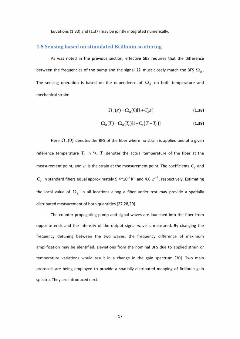
methods [45,46,47,48]: the acoustic wave is first stimulated by a long, weak pump pedestal,

and subsequently addressed by a short and intense pulse. In this manner, the transition time

of the amplification event is limited by that of the pump pulse, and not by the generation of

the acoustic wave. A spatial resolution of 5 cm has been achieved over 5 km range ([48], see

Fig. 8). Non-local effects must be carefully considered in such setups. Another principle,

which is arguably the most successful to-date, is based on differential pulse pair acquisition.

This principle is directly relevant to this research, and it is introduced next.

Figure 8. (a) Measured SBS gain map as a function of position and of frequency detuning between pump and signal. The 5 cm segment is too short to be distinguished; (b) Magnified view of the gain map around the 5 cm fiber section, showing that this segment at end of the 5 km fiber is fully resolved both in space and frequency

[48].

1.6.2 Differential double pulse pair measurements

In double pulse pair (DPP) B-OTDA setups the basic experiment is repeated twice,

and the two experiments differ slightly in the duration of pump pulses. The two raw traces

24

of the output signal power as a function of time are subtracted. Subtraction removes the

common terms, and retains only the signal amplification across a short segment that

corresponds to the difference T in pulse durations [49]. Repeating the process over a

range of values leads to the reconstruction local Brillouin gain spectra with high spatial

resolution, which is not restricted by the absolute durations of pump pulses or the acoustic

lifetime. The differential signal is typically weak, and provides low SNR. Nevertheless, B-

OTDA experiments have reached a spatial resolution of 2 cm over 2 km of fiber ([50], see

Figs. 9-11). A DPP B-OTDA experiment with distributed Raman amplification achieved 0.5 m

spatial resolution over 100 km of fiber [51].

Figure 9. Illustration of time traces of the Brillouin signal in the beginning of a fiber under test, taken with 8 ns and 8.2 ns pulse widths, and their differential signal [50]

25

Figure 10. Measured time traces of the Brillouin signal at the output of a 2 km long fiber, taken with a pulse pair of 8 ns and 8.2 duration, and the difference between the two traces [50].

Figure 11. Measured Brillouin gain spectra (top) and Brillouin frequency shift (bottom) as a function of position, towards the end of a 2 km long fiber. Measurements were taken using a double pulse pair B-OTDA setup. A 2 cm-long fiber segment was locally heated to 76 °C. The segment is identified in the measurements

[50].

26

DPP B-OTDA experiments can, at least in principle, address the entire fiber under

test in just two scans per choice of . On the other hand, the measurements require

broadband detection, at 10 GHz bandwidth for 1 cm resolution, which elevates noise levels.

In addition, pump pulses are subject to depletion over the entire length of the fiber. An

alternative SBS sensing paradigm relies on manipulating the cross-correlation function

between the complex envelopes of the pump and signal waves. Such protocols are

addressed in the following section.

1.6.3 Brillouin optical correlation domain analysis

Brillouin optical correlation domain analysis (B-OCDA) was first proposed in the late

1990's, in attempt to confine the SBS interaction and improve spatial resolution of SBS

sensing to segments that are much shorter than 1 m. The original scheme, devised by the

group of Prof. Hotate of the University Of Tokyo, relied on the synchronized frequency

modulation of the pump and signal by a common sine-wave pattern. Due to the modulation,

the frequency difference between the counter propagating pump and signal waves

remained stationary at particular fiber locations only, known as correlation peaks, whereas

the frequency difference elsewhere was oscillating [52,53]. Consequently, effective SBS

amplification was restricted to the correlation peaks, and signal power measurement could

convey localized information.

The width of the correlation peaks defined the spatial resolution of the

measurements [53,54]. In off-peak locations the stimulation of the acoustic field is largely

inhibited, and the average of the acoustic field magnitude is zero. Nevertheless, the

instantaneous magnitude of the acoustic wave in off-peak positions is fluctuating with non-

zero variance. These residual, unintended Brillouin interactions contribute measurement

noise. B-OCDA experiments based on frequency modulation achieved 24,000 high-resolution

points [55]. The highest spatial resolution reported was 1.6 mm [56].

27

Figure 12. Illustration of spatial confinement of SBS in Brillouin optical correlation domain analysis [54].

Figure 13. (a) Fiber under test (FUT)-3 prepared by fixing standard single-mode fiber (SMF) 1 on the translation stage using epoxy. (b) Results of distributed measurement on FUT-3 with elongations of 30, 60, 90, and 120

µm. Inset, magnified view around the peak position of the 60 µm case. The 3 mm fiber section is indicated by dashed lines [56].

The spacing between correlation peaks is given by [53]:

 2 g m

cd

n f , (1.43)

where mf is the rate of frequency modulation The spatial resolution equals [53]:

               2

BB m

g m

c vz for v f

n f f

, (1.44)

28

with f denoting the span of frequency modulation. The periodic nature of

frequency modulation potentially leads to the generation of multiple correlation peaks along

the fiber under test. The maximum range of unambiguous measurements is restricted by the

separation between adjacent peaks. The initial B-OCDA scheme therefore exhibited an

inherent tradeoff between spatial resolution and the range of unambiguous measurements:

the number of resolution points that can be address without ambiguity was restricted to few

hundreds only, Bd z f . This ratio may be increased with larger frequency

modulation span f , however that span is restricted to the order of tens of GHz by

technical issues. This limitation on the number of resolution points was relaxed in

subsequent, more elaborate schemes of frequency modulation B-OCDA [57], and was

removed entirely in a protocol that was proposed in our group by Yair Antman and

coworkers [58,59]. This approach is explained in detail in the next section.

1.6.4 Phase-coded Brillouin optical correlation domain analysis

In phase-coded B-OCDA both pump and signal waves are jointly phase-modulated by

a common, high-rate pseudo random bit sequence (PRBS) [60]. As previously obtained

(section 1.4.1.2, equation 1.29), the acoustic wave magnitude as a function of time and

position along the fiber is given by:

*

1

0

*

1

0

( , ) exp( ) exp( ') ( ' ) ( ' ) '

exp[ ( ')] ( ' ) ( ' ) '

t

A A p s

g g

t

A p s

g g

z L zz t jg t t A t A t dt

v v

z L zjg t t A t A t dt

v v

(1.45)

The instantaneous driving force for the acoustic wave generation is proportional to

the inner product between the pump and probe complex envelopes. Given the above

modulation scheme, that electro-strictive driving force is held constant at specific fiber

locations where the two replicas of the modulation sequence are in correlation. The driving

force is rapidly oscillating everywhere else, at a rate that can be made much faster than the

29

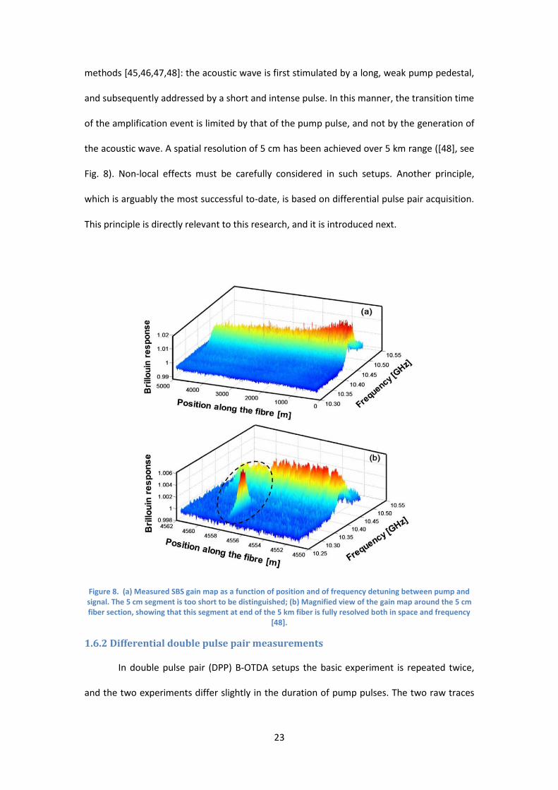
acoustic lifetime. Much like in the original B-OCDA scheme, the effective buildup of the SBS

interaction will be restricted to the correlation peaks only.

Figure 14. Illustration of counter-propagating, binary phase-coded pump and signal waves and their inner product. The two waves are correlated at the center only.

However, unlike sine-wave frequency modulation, the separation between

neighboring peaks scales with the period of the modulating sequence, which can be made

arbitrarily long. Therefore the restriction on the number of unambiguously addressed points

is removed. The width of the SBS interaction region equals half the correlation length of the

coded waveforms, or half the spatial extent of a single bit [61,62]:

1

2gz v T (1.46)

30

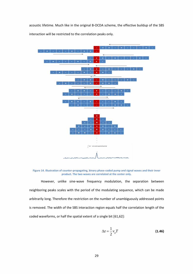
Here, T is the duration of a single bit and gv is the group velocity of light in the

fiber. A spatial resolution better than 1 cm has been reported using this method [59]. Our

group routinely performs measurements with 2 cm resolution.

Figure 15. Top left – Brillouin gain mapping of a 40-meter-long fiber with 1 cm resolution, corresponding to 4000 resolved points. A 1 cm-long section of the fiber was locally heated. Top right – magnified view of the

Brillouin gain map in the vicinity of the heated section. Bottom left – corresponding measured Brillouin frequency shift as a function of position. The region immediately surrounding the heated section is magnified in the inset. The standard deviation of this estimation along a uniform fiber section is 0.5 MHz, corresponding

to a temperature inaccuracy of ±0.5 °C. Bottom right – Brillouin frequency shift measurements over a 200-meters-long fiber, with sub cm resolution. 330 arbitrarily located sections of the fiber under test are randomly

addressed. The interrogated sections are only 9 mm long, evenly spaced by approximately 60 cm. The fiber under test consisted of two dissimilar segments spliced together. The inset shows measurements of the Brillouin shift in the vicinity of a 1 cm-long hot spot, located at the end of the fiber. (The 330 randomly

addressed sections of the main panel did not coincide with the hot spot) [59].

Two types of codes were considered in the modulation of pump and signal waves:

PRBSs and so-called perfect Golomb codes. The drawback of using PRBSs is the

comparatively large off-peak values of their auto-correlation functions [63]. Consequently,

the undesired, residual off-peak Brillouin interactions are relatively strong. Alternatively,

perfect Golomb codes, invented by Prof. Solomon Golomb of the University of Southern

California, are characterized by zero sidelobes of the cyclic auto-correlation function [63].

Use of these codes, instead of PRBSs, could be expected to reduce stimulation of the

31

acoustic field in off-peak locations. As seen in equation 1.46, the acoustic wave buildup is

given by integration over the electro-strictive driving force within an exponential window.

That exponential window takes away from the perfect correlation properties of Golomb

code [58,63]. Nevertheless, they still lead to weaker off-peak SBS interactions than those

obtained with PRBS modulation.

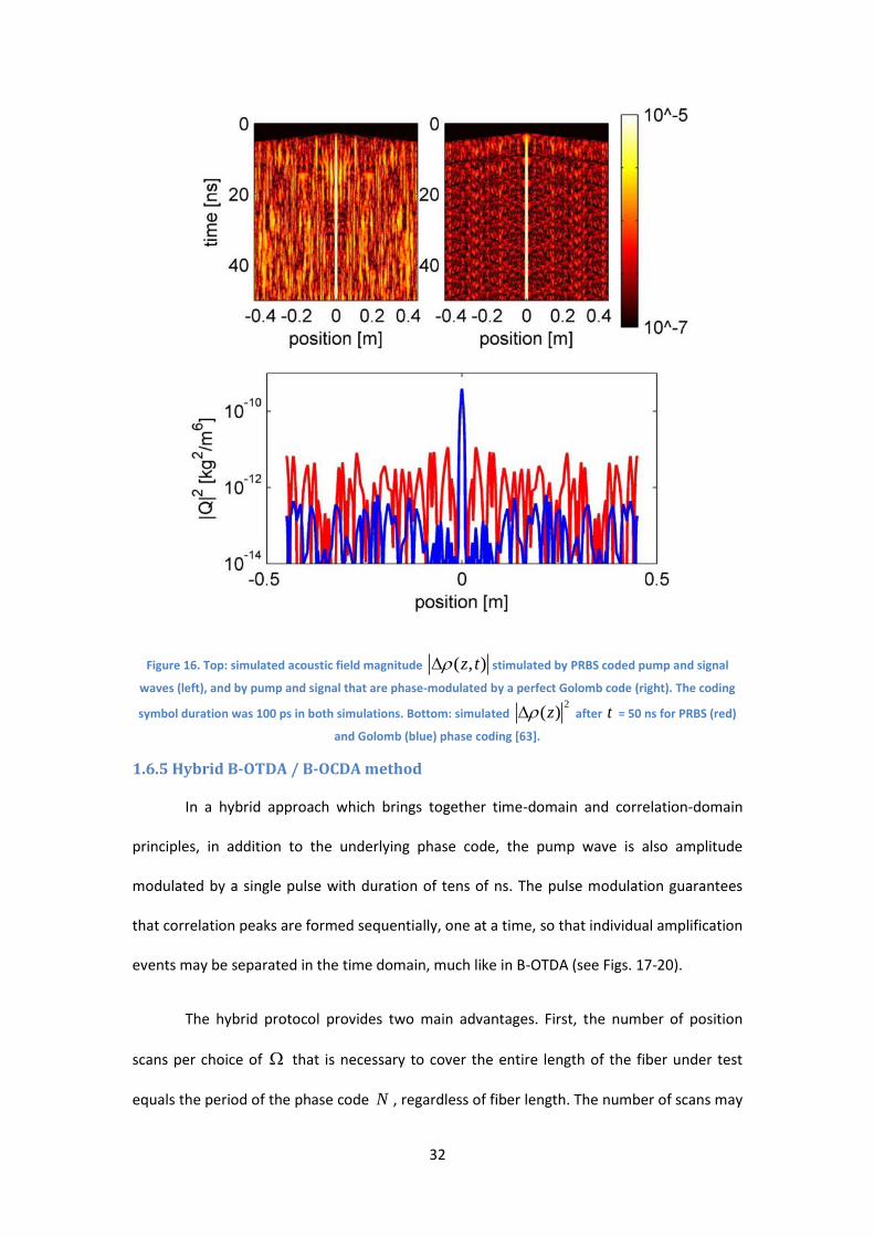
Figure 16 below shows numerical calculations of the acoustic wave magnitude as a

function of time and position along the fiber. Both a PRBS (top left) and a Golomb code (top

right) were used. Both sequences effectively confine the stimulation of the acoustic wave to

a discrete and narrow correlation peak at the fiber center (2 cm width in this case), where it

is stationary. However, the two maps differ in the extent of the off-peak acoustic wave

stimulation. Off-peak, residual stimulation is much reduced when a Golomb code is used in

the phase modulation of the optical waves.

A major drawback of B-OCDA methods is the need of spatial scanning of correlation

peak positions, one resolution point at a time. Such scanning of thousands of points, using

standard laboratory equipment, is often impractical. In order to reduce the scanning time,

the phase code period may be shortened. Thus multiple correlation peaks would be

obtained, separated by 12 gZ N v T where N is the code period. At first glance, it

appears as though the generation of multiple correlation peaks along the fiber would be a

disadvantage: measurements will become ambiguous, just like in the original B-OCDA

concept. The solution to that problem was found in the combination between time and

correlation domain analyses principles, as discussed in the next section.

32

Figure 16. Top: simulated acoustic field magnitude ( , )z t stimulated by PRBS coded pump and signal

waves (left), and by pump and signal that are phase-modulated by a perfect Golomb code (right). The coding

symbol duration was 100 ps in both simulations. Bottom: simulated 2

( )z after t = 50 ns for PRBS (red)

and Golomb (blue) phase coding [63].

1.6.5 Hybrid B-OTDA / B-OCDA method

In a hybrid approach which brings together time-domain and correlation-domain

principles, in addition to the underlying phase code, the pump wave is also amplitude

modulated by a single pulse with duration of tens of ns. The pulse modulation guarantees

that correlation peaks are formed sequentially, one at a time, so that individual amplification

events may be separated in the time domain, much like in B-OTDA (see Figs. 17-20).

The hybrid protocol provides two main advantages. First, the number of position

scans per choice of that is necessary to cover the entire length of the fiber under test

equals the period of the phase code N , regardless of fiber length. The number of scans may

33

be therefore reduced by a factor of several hundreds. Second, off-peak acoustic waves, at

any given moment, are restricted to the spatial extent of the pump pulse (which is on the

order of few meters), rather than span the entire fiber which may be many km long. This

property of the hybrid protocol strongly reduces measurement noise due to off-peak

interactions. This method was first proposed and implemented by David Elooz et al. [64,65],

within our group. Using this protocol, they were able to address 80,000 points with spatial

resolution of 2 cm over 1.6 km of fiber, using only 127 position scans [66].

Figure 17. Illustration of phase-coded BOCDA with an overlaying pump pulse. The acoustic field is stimulated at a single correlation peak only at any given instance.

34

Figure 18. Simulated magnitude of the acoustic wave density fluctuations (in normalized units), as a function of position and time along a 6 m-long fiber section. Both pump and signal waves are co-modulated by a perfect Golomb phase code that is 127 bits long, with symbol duration of 200 ps. The pump wave is further modulated by a single amplitude pulse of 26 ns duration. The acoustic field, and hence the SBS interaction between pump and signal, is confined to discrete and periodic narrow correlation peaks. The peaks are built up sequentially

one after another with no temporal overlap [66].

Figure 19. Simulated output signal power as a function of time. The trace consists of a series of amplification peaks, each of which can be unambiguously related to the SBS interaction at a specific correlation peak [66].

35

Figure 20. Measurements of the output signal power as a function or time, following propagation in a 400 m-long fiber under test that was consisted of two sections, each of about 200 m in length. The Brillouin frequency

shifts of the two segments at room temperature were 10.90 and 10.84 GHz, respectively. Multiple peaks are evident, each corresponding to the SBS amplification in a specific correlation peak of the Golomb code. A 5 cm-

long hot spot was located towards the output end of the pump wave. In both panels, one of the correlation peaks is in spatial overlap with the hot spot. The frequency offset between the pump and signal was set to

match the Brillouin shift of the second section at room temperature (panel (a), 10.84 GHz), and the Brillouin shift at the temperature of the hot spot (panel (b), 10.89 GHz) [66].

Compared with DPP B-OTDA, the hybrid measurement protocol can rely on low-

bandwidth detection that is less noisy. In addition, depletion of pump pulses is restricted to

the correlation peaks which make up a small fraction of the fiber length, and phase

modulation effectively suppresses spontaneous Brillouin scattering of the pump wave. More

advanced versions of the protocol successfully addressed 440,000 resolution points [67], and

demonstrated the potential of addressing over two million points [68]. On the other hand,

the hybrid time/correlation domain setups still require N ~ 100 position scans, as opposed

to only two in DPP B-OTDA. This number of scans remains a main drawback of all B-OCDA

variants to-date.

1.7 Research objectives

As noted above, the separation between neighboring correlation peaks in the hybrid

B-OTDA / B-OCDA schemes must exceed the spatial extent of the pump pulse, or else

measurements of the output signal power become ambiguous. The pulse duration, in turn,

must be longer than twice the acoustic lifetime 2 ~ 10 ns. Given typical symbol duration of

36

200 ps (representing 2 cm resolution), the number of scans cannot be reduced below the

order of 50-100.

As a possible extension of the previous measurement protocols, I propose herein to

bring together the principles of phase-coded B-OCDA and of DPP B-OTDA. In this method we

overlay the double-pulse architecture on top of phase-coding of pump and signal. The

duration of pump pulses in each individual experiment would exceed the phase coding

period, hence the amplification events taking place at neighboring correlation peaks would

overlap in time. However, like in DPP B-OTDA, each trace will be acquired twice with

different pump pulse duration. The difference between the two pulse durations would be

shorter than the phase coding period. Therefore, subtraction of the two output traces would

unambiguously recover the amplification taking place at each individual peak.

The benefit of the proposed principle is in reducing the number of scans: the phase

code period may be shortened to a fraction of , representing N ~ 10 position scans. The

proposed method would carry a penalty in SNR: the required detection bandwidth would be

broader than that of current B-OCDA protocols, although still not as broad as that of DPP B-

OTDA. The main tasks of my research have been the quantitative analysis and the

experimental demonstration of this DPP B-OCDA approach, and the assessment of its

performance limitations.

37

2. Principle of operation, analysis and simulations

2.1 Rationale and principle of operation

In the proposed method of this research program the hybrid B-OTDA / B-OCDA

protocol will be executed twice, with pump pulse durations of pulseT on the order of 30 ns,

and pulse pulseT T with a duration increment on the order of 1 ns. In each experiment, the

phases of the pump and probe waves will be modulated with the same Golomb code with

symbol duration phaseT , which is on the order of hundreds of ps. The complex envelopes of

the pump and signal waves can be express as:

0

, rectphase

s s s n

n phase

t nTA z L t A t A c

T

(2.1)

0

0, rect rectphase

p p p n

npulse phase

t nTtA z t A t A c

T T

(2.2)

where 0sA ,

0pA denote the constant magnitudes of the signal wave and of pump

pulses, respectively, rect( )t equals 1 for 0.5t and zero elsewhere , and nc are the

elements of the prefect Golomb code, which is repeating with a period of phaseN = 11 bits.

The magnitudes of all elements in the code are unity. The phases of elements {1,2,3,5,6,8}

equal zero, whereas the phases of elements {4,7,9,10,11} are given by

1cos 1 1phase phaseN N ~ 2.556 rad.

The temporal period of the phase code phase phaseN T is deliberately chosen to be

much shorter than the pump pulse duration pulseT , unlike previous implementations of

hybrid B-OCDA / B-OTDA [65]. Consequently, each individual measurement will be

ambiguous, in the sense that the output probe wave power at any given instance will be

affected by SBS interactions taking place at multiple correlation peaks of the underlying

38

phase code. However, subtraction of the two traces would recover 'transitions instances', in

which the longer pump pulse excites an extra correlation peak which is not covered by the

shorter one. The difference trace may therefore remove the ambiguity in data analysis.

While two scans would be necessary for each position of peaks, the reduction in code period

length could be ten-fold, and the overall experimental duration might be reduced. An

illustration of the method can be seen in the figure below.

Position

Correlation peaks

Time

Time

Back-scattered pump wave

Trace diffrential

Subtraction

pulseT

pulse pulseT T

Figure 21. Illustration of the extent of pump pulses in the two experiments of the proposed measurement protocol (left), the back-scattered pump wave as a function of time in the two cases (upper right), and the

difference trace as a function of time (lower right).

Unlike the DPP B-OTDA method, the spatial resolution of this protocol is not

determined by the time difference between two pulses, but rather by the symbol duration

of the underlying phase code: 12 g phasez v T . The subtraction of the two traces is meant to

resolve between events separated in time by phase phaseN T .

2.2 Simulations results

The proposed measurement principle is supported by direct numerical integration of

the differential equations of SBS, subject to the appropriate boundary conditions described

above. First, the previous protocol of hybrid B-OTDA / B-OCDA was simulated as a reference.

The calculated map of the acoustic field as a function of position and time, and the

39

calculated temporal trace of the output signal power, are shown in Fig. 22 and Fig. 23,

respectively. The symbol duration phaseT was 267 ps, corresponding to resolution z of 2.7

cm. The period of the perfect Golomb code was phaseN = 83 bits. The duration of the pump

pulse pulseT was 22 ns. Three correlation peaks are obtained along the 8.1 m-long fiber

under test.

Figure 22. Simulation of the acoustic wave magnitude as a function of time and position along a fiber under test, when the pump and signal optical waves are jointly phase-modulated by a periodic perfect Golomb code. The pump wave is further modulated by a single pulse, whose 22 ns duration is shorter than the period of the phase code. The acoustic field is stimulated in three discrete correlation peaks, in a sequential manner: each

interaction decays before the next one begins.

Figure 23. Simulation of the output signal power as a function of time, corresponding to the acoustic field map of the previous figure. Three distinct amplification events are obtained.

40

The calculated magnitude of the output signal wave was averaged over phaseN = 83

realizations of the B-OCDA boundary conditions. The same sequence was used in the phase

modulation of pump and signal in all calculations, however the sequence was offset by an

arbitrary number of bits 00 phasen N in each repetition [69]. The random offset helps to

average out noise due to residual Brillouin interactions at off-peak fiber locations. An

arbitrary starting point 0n of the phase modulation at 0t is inherent to the experimental

setup, since the waveform generators used in phase and amplitude modulation of pump

and/or signal are free-running without synchronization.

Next the simulation was extended to the double-pulse B-OCDA protocol. The

boundary conditions for the modulation of pump and signal were similar to those of the

previous analysis, with the following differences: the period of the Golomb code was 11 bits

(or 2.9 ns), and duration of the pump pulses were pulseT = 29 ns and pulse pulseT T = 30 ns.

The duration of the phase code symbols phaseT remained 267 ps. With these parameters, the

acoustic wave is stimulated at many correlation peaks along the fiber under test on any

given instance. Figure 24 shows the calculated acoustic wave magnitude as a function of

time and position along the fiber under test for the longer pump pulse.

The left panel of figure 25 shows the output signal wave as a function of time in both

calculations, and the right panel shows the result of the subtraction of the two traces. Since

pulse phase phaseT T N , multiple gain events are in temporal overlap. Following an initial

transient, the output signal power at any given instance is affected by SBS interactions

taking place at multiple peaks. Hence, individual amplification events cannot be directly

resolved without ambiguity. However, due to the difference in duration between the pump

pulses used in the two traces, there are specific instances in which the longer of the two

pulses excites a given correlation peak while the shorter one does not. The SBS amplification

41

at that particular peak appears as an isolated event in the difference trace of the output

signal, at that particular time.

Figure 24. Simulation of the acoustic wave magnitude as a function of time and position along a fiber under test, when the pump and signal optical waves are jointly phase-modulated by a perfect Golomb code with a shorter period of only 2.9 ns (11 bits). The pump wave is further modulated by a single pulse, whose 30 ns

duration is longer than the period of the phase code. The stimulation of the acoustic wave at numerous peak positions overlaps in time.

Figure 25. The left panel shows simulations of the Brillouin gain of the output signal wave as a function of time, in the two traces of the proposed double-pulse B-OCDA scheme. The right panel shows the difference between

the two traces as a function of time. Brillouin interactions at individual correlation peaks are resolved.

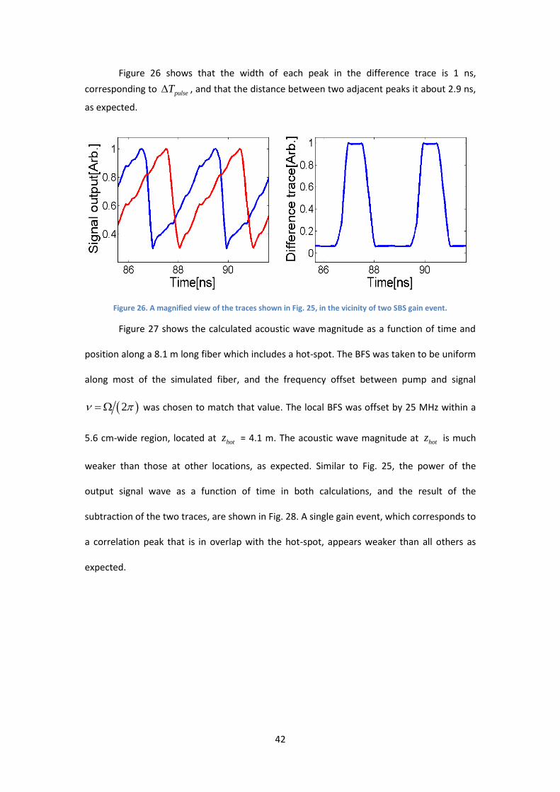
42

Figure 26 shows that the width of each peak in the difference trace is 1 ns,

corresponding to pulseT , and that the distance between two adjacent peaks it about 2.9 ns,

as expected.

Figure 26. A magnified view of the traces shown in Fig. 25, in the vicinity of two SBS gain event.

Figure 27 shows the calculated acoustic wave magnitude as a function of time and

position along a 8.1 m long fiber which includes a hot-spot. The BFS was taken to be uniform

along most of the simulated fiber, and the frequency offset between pump and signal

2 was chosen to match that value. The local BFS was offset by 25 MHz within a

5.6 cm-wide region, located at hotz = 4.1 m. The acoustic wave magnitude at hotz is much

weaker than those at other locations, as expected. Similar to Fig. 25, the power of the

output signal wave as a function of time in both calculations, and the result of the

subtraction of the two traces, are shown in Fig. 28. A single gain event, which corresponds to

a correlation peak that is in overlap with the hot-spot, appears weaker than all others as

expected.

43

Figure 27. Calculated normalized magnitude of the stimulated acoustic field as a function of position and time along a 8.1 m long fiber under test. Only part of the fiber is shown, for better clarity. The BFS of the fiber was taken to be uniform, and the frequency offset between pump and signal was chosen to match that value. The

BFS was modified by 25 MHz within a 5.6 cm-wide segment located 4.1 m from the input end of the pump wave. The signal and pump waves are jointly phase-modulated by a repeating perfect Golomb code with a

period of 11 bits and symbol duration of 267 ps. The pump wave is also amplitude-modulated by a single pulse of 30 ns duration. The acoustic field is confined to multiple, discrete and closely-spaced correlation peaks. Due

to the short period of the phase code, SBS interactions at neighboring peaks take place with substantial temporal overlap. The acoustic field at the peak which is in spatial overlap with the modified region is

considerably weaker than all others.

Figure 28. Left - calculated power of the signal wave at the output of the FUT. Red and blue traces correspond to pump pulse durations of 30 ns and 29 ns, respectively (see legend). Right-the difference between the two traces as a function of time. Brillouin interactions at individual correlation peaks are resolved. The gain event which corresponds to a correlation peak that is in overlap with the fiber region of modified BFS appears much

weaker than all others.

In the following simulation, the value of the BFS at the location of one of the

correlation peaks was modified by several detuning values. The frequency difference

44

between pump and signal was kept equal to the 'nominal' value of the BFS in the rest of the

simulated fiber. The calculated difference traces are shown in Fig. 29 below. The magnitude

of the signal gain in the difference trace at that particular peak is seen to decrease with

detuning, as expected.

Figure 29. Simulated difference traces of double-pulse B-OCDA. The value of the Brillouin shift at the location of the tenth peak from the left was detuned from its nominal value. Detuning values were: 0 MHz, 10 MHz,

and 20 MHz in the blue, red and black traces, respectively. The magnitude of the specific gain peak in the difference trace decreases with detuning, as expected.

The main advantage of the proposed DPP B-OCDA protocol, with respect to the

previous realizations of B-OCDA mentioned above, is the number of position scans required

to address the entire FUT. Figure 30 compares between the maps of the acoustic field

magnitudes obtained with a 11 bits-long Golomb code and a 83 bits-long PRBS. The symbol

duration of the phase codes is the same in both calculations. The shorter code leads to the

stimulation of SBS in a larger number of peaks.

45

Figure 30. Calculated normalized magnitude of the stimulated acoustic field as a function of position and time along a 8.1 m long fiber under test. Both pump and signal are phase-modulated by repeating codes, with a

symbol duration of 267 ps. The pump wave is also amplitude-modulated by a single pulse of 30 ns duration. The phase sequences used are perfect Golomb codes with period of 11 bits (left), and a PRBS with a period of

83 bits (right).

2.3 Signal to noise ratio

2.3.1 Noise mechanisms

So far, the calculations of the signal wave at the output of the fiber under test were

carried out under to the assumption that the signal was noise-free. The only noise

mechanism that was inherent to the analysis was residual off-peak Brillouin interactions due

to the imperfect periodic correlation of Golomb codes subject to an exponential weighing

window [58]. However, our experiments below made use of very short codes, with a period

of only 11 bits, so that phase phaseN T . At that limit, off-peak interactions are strongly

suppressed.

In practice, the detection process includes inevitable shot noise, the measurement

photo-current is accompanied by additive thermal noise, and the detected waveform itself

may include amplified spontaneous emission (ASE) from fiber amplifiers along the path of

the signal wave. These noise mechanisms are briefly addressed in this section, and an

estimate of their effect on the measurement precision is given as well.

46

2.3.1.1 Noise due to amplified spontaneous emission of fiber amplifiers

Brillouin sensing setups draw both pump and signal waves from a common laser

diode source. Splitting losses and insertion losses of multiple fiber-optic components, (see in

next chapter), typically require that both waves are amplified along their respective paths,

using either semiconductor optical amplifiers (SOAs) or erbium-doped fiber amplifiers

(EDFAs). Optical amplification is inevitably accompanied by broadband ASE, which spans the

entire gain bandwidth of the amplifiers (on the order of few THz). Narrowband optical band-

pass filters are used to restrict the noise bandwidth as much as possible, to a residual

bandwidth optB . The optical power of the filtered ASE is given by:

( 1)ASE n optP F hv G B . (2.3)

Here G ~ 300 represents the power gain of the optical amplifier, nF ~ 5 denotes the

noise figure of the amplifier, and h = 1.28e-19 J is the photon energy at 1550 nm

wavelength. For optB of about 10 GHz, ASEP is on the order of 2 µW (-27 dBm). For

comparison, the power of the amplified signal wave going into the detector, sP , is typically

on the order of 100 µW (-10 dBm).

Let us define ASESNR as the ratio between the average photo-current squared,

achieved in the detection of sP , and the variance in the photo-current that is induced by

ASEP . When using a narrow-band filter optB , the primary noise term in the photo-current is

due to the beating between the optical field of the SBS signal wave and the optical field of

ASE (a term known as signal-spontaneous beating [70]). Let us assume that the electrical

bandwidth of the detector and its associated circuitry is ElectB ~ 0.7 GHz. In this condition,

ASESNR may be approximated by [71]:

47

2 ( 1)

sASE

n Elect

PSNR

F hv G B

. (2.4)

The SNR due to ASE is on the order of 350.

2.3.1.2 Shot noise

Shot noise stems from the quantum nature of the photo-detection process. The

collected photo current consists of a series of elementary charges e , each generated in

response to the absorption of a single photon. The timing of each event is random, and

uncorrelated with those of other events. The number of charges N collected within any

finite duration detT therefore becomes a random variable. It can be shown that N obeys

Poisson statistics [71]:

( ) exp( )!

N

Np N N

N , (2.5)

which is entirely defined by its mean value:

det sPTN

h

. (2.6)

Here is the quantum efficiency of the photo-receiver. It can be verified directly

that the expectation value of N is indeed N , and that its variance also equals N .

Therefore, the SNR associated with shot noise equals:

det

2

s sShot

Elect

PT PSNR

h h B

. (2.7)

Here we denoted the electrical bandwidth associated with photo-detection over

duration detT by det1 2ElectB T . ElectB is on the order of 1 GHz. A comparison between

the expressions for ShotSNR and ASESNR above suggests that shot noise is negligible in

most systems that involve optical amplification.

48

2.3.1.3 Thermal noise

The current generated by the photo-detector flows along a finite load conductor of

resistance LR . Random thermal motion of free electrons in this conductor contributes noise

currents, which add to the intended, photo-detected signal. The extent of this so-called

thermal noise is independent of the detected optical power. The SNR associated with

thermal noise is given by [72]:

2

2( )(4 / )

sThermal

B L A Elect

PeSNR

h k T R F B

(2.8)

Here Bk = 1.38e-23 J/K is Boltzmann's constant, and AF ~ 10 is a noise figure

associated with the electrical amplification within the detector circuitry. Trans-impedance

photo-receivers exhibit load resistors on the order of Mega-Ohm, leading to thermalSNR in

access of 1e7 in the detection of sP above. Even with a load resistor of 50 Ohm, the SNR

associated with thermal noise in our measurements is expected to be larger than 1,000.

2.3.1.4 Overall signal-to-noise ratio assessment and its implications

The discussion of the above sections suggests that the dominant noise mechanism in

the detection of the signal wave is due to ASE. However, the expression given above for

ASESNR cannot be used directly, for the following reason: The quantity of interest in SBS

sensing is not the signal power sP itself, but rather the changes sP in sP due to SBS over a

short segment of length z . These changes are considerably smaller than sP . When the

frequency detuning between pump and signal matches the BFS, we may expect:

0 0exps s p s p sP P g P z P g P P z (2.9)

49

Here pP is the power level of pump pulses. The measurement noise in DPP B-OCDA

is increased by a factor of 2, due to the subtraction between two traces. The SNR in

measurement of the quantity of interest sP therefore may be approximated as:

2 2

0 0

2 4 ( 1)

p p s

Tot ASE

n Elect

g P z g P z PSNR SNR

F hv G B

(2.10)

The pump power in long-range Brillouin sensors experiments is limited by the onset

of modulation instability due to the interplay of Kerr effect and chromatic dispersion [72],

spontaneous Brillouin scattering and Raman scattering, to the order of few hundreds of mW.

The experiments carried out in this research involved short fiber segments, only few tens of

meters long. Even in these experiments, pP cannot be increased beyond few Watts due to

saturation of amplifiers, finite extinction ratios of modulators etc. Typical values for the gain

coefficient at standard single-mode fibers are on the order of 0g = 0.1 [Wm]-1. With z = 2

cm, the factor 0 pg P z is bound by few percent, at most. Therefore, the experimental

signal-to-noise ratio TotSNR may be as low as 0.07.

An expression relating the experimental uncertainty in the estimate of BFS and the

measurement SNR was derived by Soto and Thevenaz in 2013 [41]. The expression was given

in Chapter 1, and it is repeated here for convenience:

3 1

4 2B

B

TotSNR

(2.11)

Here = 1.5 MHz is the step-size in the scanning of the frequency offset between

pump and signal waves. Note that the SNR in the original publication was defined as the

square root of the quantity used in this discussion. The above formula suggests a very large

experimental error of ±22 MHz, which cannot be tolerated. The SNR improves, however,

with the number of repetitions avN in the acquisition of the output signal wave. 512

50

repetitions were used in our experiments. Averaging is expected to reduce the experimental

error to the order of ±1 MHz. As shown in the next chapter, the uncertainty in the

experimental BFS measurements is not far from this prediction.

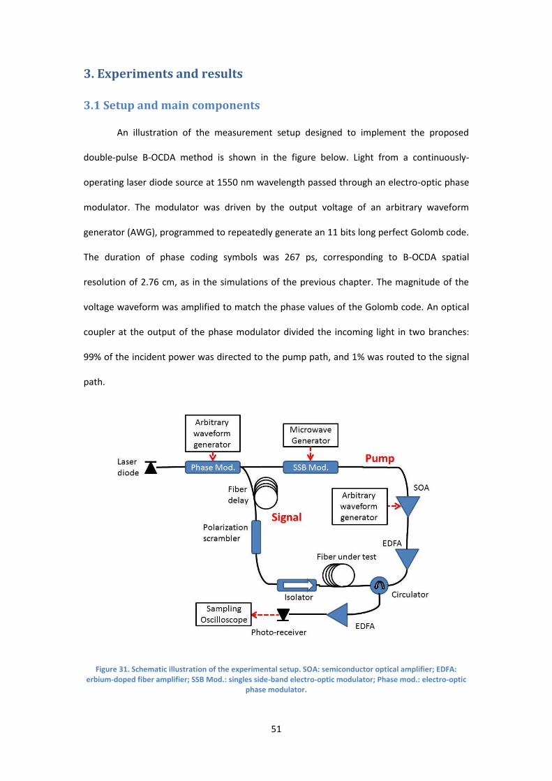
51

3. Experiments and results

3.1 Setup and main components

An illustration of the measurement setup designed to implement the proposed

double-pulse B-OCDA method is shown in the figure below. Light from a continuously-

operating laser diode source at 1550 nm wavelength passed through an electro-optic phase

modulator. The modulator was driven by the output voltage of an arbitrary waveform

generator (AWG), programmed to repeatedly generate an 11 bits long perfect Golomb code.

The duration of phase coding symbols was 267 ps, corresponding to B-OCDA spatial

resolution of 2.76 cm, as in the simulations of the previous chapter. The magnitude of the

voltage waveform was amplified to match the phase values of the Golomb code. An optical

coupler at the output of the phase modulator divided the incoming light in two branches:

99% of the incident power was directed to the pump path, and 1% was routed to the signal

path.

Figure 31. Schematic illustration of the experimental setup. SOA: semiconductor optical amplifier; EDFA: erbium-doped fiber amplifier; SSB Mod.: singles side-band electro-optic modulator; Phase mod.: electro-optic

phase modulator.

52

The signal wave propagated through a fiber path imbalance, necessary for the

precise scanning of correlation peaks positions along the section of fiber under test (see

details in section 3.1.2 below, and in [59]). The delay line was followed by a polarization

scrambler, required to eliminate polarization-induced fading of SBS in case the pump and

signal are orthogonal to each other at a particular location [36]. Lastly, the signal wave was

launched into one end of the fiber under test (FUT).

The pump wave passed through a single side-band (SSB) electro-optic modulator,

driven by a sine wave of frequency from the output of a microwave synthesizer. The

modulator was biased to provide a single offset replica of the phase modulated waveform,

centered at an optical frequency of 0 where 0 is the optical frequency of the laser

diode source. The opposite, lower sideband and the original carrier were suppressed by

about 20 dB. Light at the pump branch was amplitude-modulated by repeating, low-duty

cycle pulses in a SOA with a period of 2 µs, and amplified further by a high-power EDFA to an

average power of 0.4 W (estimated pulse peak power of about 10 W). Last, the pump pulses

were routed through a circulator into the opposite end of the FUT.

The section of fiber under test was 43 m-long. The signal wave at the FUT output

was amplified by a second EDFA, and detected by a broadband photo-receiver. An optical

bandpass filter was used to suppress the amplifier ASE. The figure below shows an image of

the measurement setup in our group laboratory.

53

Figure 32. Image of a laboratory hybrid B-OTDA/B-OCDA setup, used in DPP B-OCDA experiments.

Below are brief descriptions of the functions of major components that make up the

experimental setup.

Electro-optic modulator

In optical communication systems, the electro-optic modulator is responsible for

superimposing information onto an optical carrier wave. This information can change the

phase, amplitude, frequency or polarization of incident light. There are, therefore, several

types of modulators, categorized according the type of modulation they impose on the

propagating light wave. We use both phase and amplitude modulation in our setup.

Electro-optic phase modulator:

Phase modulation can be implemented based on the electro-optic effect in LiNbO3

crystals. In this effect, the refractive index of the material changes with the application of an

external voltage V [72]:

3

33

1 V 

2n n r

d (3.1)

54

In the above equation d is the distance between electrodes surrounding a

waveguide in the crystal, and 33r is an electro-optic coefficient of the crystal ( 33r = 30.9*10-12

[m/V]). Changes in refractive index modify the accumulation of phase along a waveguide of

length l :

3

33

π

2π π V V      πλ λ V

n l n r ld

(3.2)

Here πV is defined as the voltage necessary to induce a phase shift of π radians.

The phase modulator element also provides the basis for amplitude modulation, as

discussed next.

Electro-optic amplitude modulator:

Amplitude modulation can be realized in a Mach-Zehnder interferometer (MZI)

configuration (Fig. 33). Incoming light is split in two waveguide paths, each consisted of a

LiNbO3 phase modulator, and combined together at the output. Incident power is divided

equally between the two arms. The drive voltages for the two embedded phase modulators

are 1,2V .

Figure 33. A schematic illustration of a LiNbO3 Mach-Zehnder interferometer amplitude modulator [72]

The output field magnitude can be written as:

12 120 0

1  exp exp exp exp( )2 2 2

outE E j j j j t

(3.3)

55

Here 0E is the magnitude of the incident field with a carrier optical frequency 0 ,

1,2 are the electro-optic modulation phases at the two arms, 12 1 2( ) and

1 2

1  (   )2

. The output power is given by:

2 2 21 2

12 0 0

π

V  V1 1    1 cos   1 cos π

2 2 Vout outP E E E

(3.4)

Power transmission is complete when the two drive voltages are equal (constructive

interference between light propagated in the two arms), whereas transmission is blocked

when the difference between the two drive voltages is set to πV (destructive interference).

Single-Sideband modulation

In standard electro-optic modulators, of either phase or amplitude, modulation

introduces two spectral sidelobes, above and below the frequency of the optical carrier. In

many setups, such as ours, only a single sideband (SSB) is useful, while the complementary

sideband disrupts the measurements. Many SBS sensor setups use narrowband optical

filters to select a single sideband following modulation. Alternatively, SSB modulators

generate only an SSB to begin with. The device consists of two independent MZI amplitude

modulators, and the input electrical waveform is therefore driven twice into the device. A

phase shift of 90 must be introduced between the two replicas. In addition, the carrier

wave itself may be suppressed with a careful choice of a DC bias to the modulators.

Our setup employs an SSB modulator to generate the pump wave from a replica of

the signal. The device is driven by an electrical sine wave from a microwave generator at

frequency B , and adjusted so that only the shorter-wavelength (higher-frequency)

sideband is retained. An example is shown in the figure below. The opposite sideband and

the optical carrier are effectively suppressed, by a factor on the order of 20 dB.

56

Figure 34. An optical spectrum analyzer measurement of an optical carrier following SSB modulation by a sine wave of frequency on the order of 10 GHz. The right-hand (longer wavelength) sideband is retained, to be used

as an SBS probe wave. The optical carrier itself and the opposite sideband are largely suppressed. Note that roles were reversed in the DPP B-OCDA experiment, and the shorter-wavelength sideband was retained

instead.

3.1.1 Polarization control

Control over the state of polarization is required in several positions along the

measurement setup. First, electro-optic modulators support the propagation of one linear

state of polarization and block the orthogonal one. Manual polarization controllers (PCs)

were used to adjust the incoming polarization to the state supported by modulators.

Further, the SBS interaction itself is polarization dependent, and may vanish entirely if the

states of polarization of pump and signal are orthogonal [36].

Polarization-induced fading can be mitigated using a polarization switch: a device

that can toggle the polarization of an optical wave between two orthogonal states. The SBS

sensing experiments is carried out twice, using both polarizations, and the recorded traces

are averaged [37]. The scheme therefore implements polarization diversity. However, the

switching operation requires that at least part of the setup is constructed from polarization

maintaining fibers, a requirement we could not meet. Instead, a polarization scrambler (Fig.

35) was used to switch the instantaneous state of polarization (SOP) of the signal wave

between random states that were evenly distributed on the Poincare sphere, at a rate of

100,000 states per second [36]. The comparatively slow scrambling rate mandates that at

57

least 128 repetitions of each trace are averaged, even if the measurement SNR is otherwise

sufficient.

Figure 35. The polarization scrambler used in the experimental setup.

3.1.2 Scanning of correlation peaks positions

The intuitive approach to shifting the positions of correlation peaks would be to

introduce a variable delay to the phase coding of either pump or probe waves in increments

of a single bit. This solution would require the separate and synchronous modulation of the

two waves with two phase modulators. Alternatively, the positions of correlation peaks can

be moved through slight modifications to the exact bit duration. An illustration is provided in

Fig. 36.

Figure 36. Illustration of shifting the position of correlation peaks through small-scale changes to the exact bit duration.

The FUT and the fiber paths leading to it from the input ends of the pump and signal

form a fiber loop. A so-called zero-order correlation peak is formed at the center of that

58

loop, in a position denoted below as 0z . Multiple, higher-order correlation peaks are

formed at positions 12m phase gz m N v T , where m is a positive or negative integer. The

locations of all these peaks, other than 0m , change with symbol duration:

phase phasem

m phase phase

T fz

z T f

(3.5)

Here phasef represents a variation of the clock rate

phasef driving the phase

modulator, and phaseT is the corresponding variation in the symbol duration phaseT .

A proper B-OCDA experiment requires that the offsets mz in the exact positions of

all correlation peaks mz are equal. However, the precise offsets depend on m . Differences

may be arbitrarily reduced when a long delay line imbalance is placed in either the pump or

the signal paths. The path imbalance guarantees that high-order peaks are in overlap with

the fiber segment of interest: 1m . Let us denote the length of the fiber under test as L ,

and that of the delay line as delayL . The location of the point of measurement that is nearest

to the center of the loop is:

1

2

delayL Lz

(3.6)

The clock-rate increment that is necessary to achieve z resolution at that position

is given by:

1

1

2phase phase

delay

f z f zf

z L L

(3.7)

Similarly, the measurement point that is the most further away from the center is

located at:

2

2

delayL Lz

(3.8)

The offset in that location subject to the above 1f would be:

59

22

1

Delay

Delay

L Lzz z z

z L L

(3.9)

Near-uniform scanning of positions therefore requires that delayL L . A 2.2 km-

long fiber path imbalance was used in our experiments, alongside a 43 m-long FUT. The

phase modulation clock rate phasef was 3.75 GHz, and the necessary step size

phasef for a

spatial resolution of 2.67 cm was 92.764 kHz.

3.2 Results

In a proof-of-concept DPP B-OCDA experiment, the entire FUT was scanned using

phaseN = 11 positions of correlation peaks. For each set of positions, the frequency difference

2 between pump and signal was scanned between 10.72 GHz to 10.82 GHz in 1.5

MHz steps. A pair of traces was recorded at each frequency, using pump pulses of pulseT =

30 ns or pulse pulseT T = 29 ns duration as discussed in the previous chapter. Each trace was

averaged over 512 repetitions. The photo-current from the detector at the output signal

path was sampled by a real-time, digitizing oscilloscope at 5 GHz bandwidth. The sampled

data was digitally filtered off-line to a bandwidth of 0.7 GHz, to improve the SNR. Three 8 cm

wide hot-spots were placed along the FUT, by attaching the fiber coil to a hot plate (see Fig.

37). The separations between the first hot-spot and the second, and between the second

and third ones, were 40 cm and 4.7 m respectively.

60

Figure 37. Image of part of the fiber under test, coiled and placed on top of a hot-plate to introduce three local hot-spots.

Figure 38 (bottom left) shows an example of a single pair of output signal traces

taken at = 10.765 GHz, a value that is close to the BFS of the FUT at room temperature.

Only parts of the complete traces are shown for better clarity. The displayed section includes

a single hot-spot. Both traces consist of series of overlapping gain events. Figure 38 (bottom

right) shows the result of the subtraction between the two traces. The difference trace

consists of a series of individual gain events that are separated by phase phaseN T = 2.9 ns. The

duration of each event is pulseT = 1 ns, and it represents the SBS amplification in a single

correlation peak of width z . Measurements are resolved even though the temporal

separation between adjacent peaks is shorter than the Brillouin lifetime, and much shorter

than the pump pulses durations. A single gain event, which corresponds to a correlation

peak that is in overlap with the location of the hot-spot, appears much weaker than all

others. Note the similarity between the experimental, bottom panels of Fig. 38 and the

simulated results (Fig. 28, repeated at the top panels of Fig. 38 for convenience)..

61

Figure 38. Bottom Left – example of a pair of measurements of the output signal wave, taken for = 10.765

GHz which is close to the BFS of the FUT at room temperature. Only parts of the traces are displayed for better clarity. The sections of the traces displayed are in overlap with a single hot-spot. The pump pulse durations were 30 ns (red trace) and 29 ns (blue trace). Both traces consist of series of overlapping SBS gain events.

Bottom Right – result of the subtraction between the two traces of the left panel. The difference trace consists of a series of amplification events that are unambiguously associated with individual correlation peaks. A

single gain event, which corresponds to a correlation peak that is in overlap with the hot-spot, is much weaker [73]. The top left and top right panels present the results of a corresponding simulation (repeat of Fig. 28).

The magnitude of the SBS gain at each peak was estimated as follows: the

instantaneous maximum reading of each gain event in the difference trace of Fig. 38 (right)

was identified, and the trace was integrated over a 1 ns-wide window centered at that

maximum. Upon completion of the spectral scanning over all values of , the position of all

correlation peaks were shifted by z as explained above and the spectral scan was carried

out again. The correlation peaks returned to their original location following 11 shifting

steps.

Figure 39 shows the measured SBS amplification as a function of frequency offset

and position z . The SBS gain map consists of 1,600 resolution points that were addressed

using only 11 pairs of traces per choice of . The entire FUT was covered in the

measurements. A magnified view of the SBS gain map in the region containing the three hot-

62

spots is provided in Fig. 40. The three hot spots are clearly identified at positions around 28

m and 33 m.

Figure 39. Measured normalized SBS gain (arbitrary units), as a function of correlation peak position and frequency offset

between pump and signal waves [73].

Figure 40. Magnified view of Fig. 39, in the vicinity of the three hot-spots.

Finally, Fig. 41 (left) shows the measured BFS as a function of position. Magnified

view of the fiber segment containing the three hot-spots is provided in Fig. 41 (right). All

three hot-spots are identified in their correct locations.

63

Figure 41. Measured Brillouin frequency shift as a function of position. Right – magnified view of the region containing the

three local hot-spots [73].

The experimental error in the measurement of the BFS can be evaluated based on

the variations between its values in adjacent resolution cells [65]:

2

12 B B

z

z z z (3.10)

where z

denotes averaging over position z . of the experiment equals ±1.9

MHz. This value is not far from the estimate given in chapter 2, based on SNR considerations.

The evaluation assumes that changes in the measured BFS over short segments of z

length, outside the hot-spots, represent measurement noise rather than physically

meaningful variations. This evaluation of the experimental error therefore represents a

pessimistic upper bound. The experimental error increased to 3 MHz when the number of

averaged acquisitions of each trace was reduced from 512 to 256.

64

4. Summary and discussion

The motivation for my research has been to try and reduce the number of position

scans necessary in phase-coded B-OTDA by an order of magnitude. We were able to do so

through the combination between B-OCDA and DPP acquisition principles. The

measurement protocol is an extension of previous, time-gated B-OCDA setups, in which both

pump and signal waves are jointly modulated by a repeating, high-rate phase code and the

amplitude of the pump wave is also modulated by a pulse. The phase code was short, and its

period was much shorter than the duration of pump pulses. Hence SBS was stimulated in a

large number of correlation peaks in each trace. However, individual gain events overlapped

in time. Unambiguous measurements were recovered by taking each trace twice, with pump

pulse durations that slightly differed, and subtracting the two traces of the output signal.

The number of positions scans that is necessary to cover the entire FUT equals the number

of bits in the phase code, and it is independent of the fiber length.

In a proof-of-concept experiment, a 43 m-long FUT was analyzed with a spatial

resolution of 2.7 cm. All 1,600 resolution points were addressed using only 11 scans of the

correlation peaks positions, the smallest number of any B-OCDA experiment. Previous B-

OCDA setups required at least 50-100 position scans, and sometimes even thousands of

scans. The accuracy in the measurement of the BFS was 1.9 MHz. Three local hot-spots were

properly identified in the measurements. The spacing between adjacent peaks positions was

only 30.4 cm. Such close spacing cannot be applied in direct, single-pulse B-OCDA due to

acoustic lifetime limitations.

4.1 Comparison with other Brillouin sensing protocols

The DPP B-OCDA setup represents a middle-ground between earlier, time-gated B-

OCDA protocols [65,74,69,68] and DPP B-OTDA [50], with respect to the trade-off between

SNR and number of position scans. Previous B-OCDA protocols of cm-scale resolution

65

required at least 100 scans of correlation peaks positions to cover the entire FUT, but on the

other hand typically involved detection at 100 MHz bandwidth or lower. The measurements

reported in this work required only 11 pairs of position scans, with detection at 0.7 GHz

bandwidth. On the other extreme, DPP B-OTDA covers the entire FUT with a single pair of

scans, but requires detection at several GHz bandwidth [50]. A similar trend may be

expected with respect to pump depletion. The pump pulse is depleted along the entire

length of the FUT in DPP B-OTDA. Depletion is confined to a shorter effective length

phaseL N in DPP B-OCDA, and to a length that is shorter still in previous time-gated B-OCDA

setups.

The uncertainty in the BFS estimate of all three protocols is governed by the SNR of

the SBS gain measurement [74]. In systems that are limited by shot noise, additive detector

noise or amplifier noise, the SNR scales inversely with the detection bandwidth. The

degradation in SNR must be compensated by a larger number of repetitions avN in the

averaging of each trace. Therefore, subject to equal power levels of pump and signal, similar

amplifier and detector noise performance and the same spectral scanning, DPP B-OCDA

should require fewer averages than DPP B-OTDA, but more averages than previous time-

multiplexed B-OCDA setups. Noise due to residual off-peak SBS interactions is expected to

be lower in the DPP B-OCDA measurements than in previous B-OCDA setups, due to the use

of shorter perfect codes.

In principle, the overall number of traces required to achieve a given precision:

namely the product of avN , the number of frequency offset values and the number of

positions scans, should be similar for all three protocols. The preference of one approach

over others would depend on convenience and on availability of components. In some

practical systems, however, other considerations might mandate a certain minimum number

of avN . For example, in our experiment the averaging over 512 repeating acquisitions was

66

required due to the operation rate of the polarization scrambler. Use of polarization

switching [37,68], or polarization diversity schemes [76], is expected to reduce this number.

Both time-multiplexed B-OCDA and DPP B-OTDA have reached a measurement

range of several km with cm-scale resolution, addressing hundreds of thousands of points

[50,65,74,77,69,68]. There is no fundamental limitation that should prevent the currently

proposed DPP B-OCDA principle from reaching comparable range. However, these efforts

are beyond the scope of the present work.

4.2 Limitations

The measurement parameters of DPP B-OCDA are restricted by several

considerations. The duration of pump pulses pulseT must be several times longer than the

acoustic lifetime: on the order of 25 ns or longer, so that the stimulated acoustic fields at the

correlation peaks positions may reach their maximum, steady-state values. The specific

choice of 30 ns, however, was arbitrary.

The difference between the durations of the two pulses used in each measurement,

pulseT , must be shorter than the phase code period phase phaseT N , or else the analysis of the

difference trace would become ambiguous as well. The electronic bandwidth of the

detection circuitry, ElectB , must be broad enough to accommodate gain events of duration

pulseT . Hence, choice of a short pulseT would unnecessarily increase the detection

bandwidth and measurement noise. An arbitrary value of 1 ns was used in this research.

Given the code period phase phaseT N of 2.9 ns, a larger difference between pulse durations

could have been used. Optimization of pulseT and ElectB was not carried out within the

scope of this research. Similarly, use of even shorter phase codes would reduce the number

of positions scans necessary, but increase the detection bandwidth and elevate the noise

levels.

67

The extinction ratio in the amplitude modulation of pump pulses needs to be high.

Non-zero pedestal of pump pulses introduces undesired residual SBS interactions along the

entire length L of the fiber, which may mask out the gain provided by the pulse itself. As a

rule of thumb, the extinction ratio of pump modulation must exceed L z . Other

limitations are not fundamental, and have to do with the specific implementation chosen for

the proposed principle. The comparatively slow scrambling of polarization requires many

averages. The scanning of peaks positions through clock rate variations requires a delay

imbalance that is 10-100 times longer than the FUT.

4.3 Future work

Several improvements can be made in the implementation of the proposed

principle. The first one is the employment of polarization switching and diversity, rather than

scrambling, in the mitigation of polarization-induced fading of the local SBS interactions. Our

group had used polarization switching in other B-OCDA experiments before [38]. The

number of repetitions required in the averaging of each trace was much reduced. I expect a

similar benefit in the DPP B-OCDA setup.

Other potential improvements are the use of even shorter phase sequences, such as

a 5 bits Golomb code, to reduce the number of positions scans even further. Resolution can

also be improved, towards 1 cm. In both these cases, the detection bandwidth would have

to be broadened, and the SNR may be degraded. The number of averages is expected to

increase accordingly.

Last but not least, DPP B-OCDA can be performed over km-scale fibers, addressing

hundreds of thousands of resolution points with a small number of position scans. Previous

measurements with km-scale range and cm-resolution were limited by either pump

depletion, long measurement duration or the complexity associated with the collection and

processing of vast amounts of data. Our group previously performed B-OCDA over 8.8 km of

68

fiber with 2 cm resolution, addressing all 440,000 points. That experiment was limited by

complexity and acquisition duration. DPP B-OCDA reduces the number of position scans, and

does not involve the complicated dual-hierarchy coding scheme of our previous work, hence

its extension to an even larger number of resolution points should be feasible.

On the other hand, DPP B-OCDA is more prone to depletion than our previous

setups. Depletion takes place over an effective length of 11phaseL N L . As mentioned

earlier in this section, DPP B-OTDA experiments are susceptible to depletion over the entire

length L of the fiber under test. DPP B-OTDA was successfully carried out over 2 km with 2

cm resolution. Drawing on this previous example, it is reasonable to expect that B-OCDA

measurements could be performed over 20 km of fiber before being restricted by depletion.

As new middle-ground between previous time-domain and correlation-domain protocols,

the configuration proposed in this research has good potential to improve upon the current

state-of-the-art in terms of the number of resolution points addressed, and perhaps raise

the bar above 1 million points.

69

5. Bibliography

1. E. Udd, W. Spillman, (2011). Fiber Optic Sensors: An Introduction for Engineers and Scientists, 2nd ed., John Wiley & Sons, Inc., New Jersey.

2. J.M. López-Higuera, (2011), Handbook of optical fibre sensing technology. 1st ed., John Wiley, New Jersey, United States.

3. K.T.V. Grattan and B.T Meggit, (Springer, 2000). Optical Fiber Sensor Technology. 4. López-Higuera, J. M., Cobo, L. R., Incera, A. Q., & Cobo, A. (2011). Fiber optic

sensors in structural health monitoring. Journal of Lightwave Technology, 29(4), 587-608.

5. Tapanes, E. (2001, October). Fibre optic sensing solutions for real-time pipeline integrity monitoring. In Australian Pipeline Industry Association National Convention (Vol. 3, pp. 27-30).

6. Ravet, F., Briffod, F., & Nikles, M. (2008, January). Extended distance fiber optic monitoring for pipeline Leak and ground movement detection. In 2008 7th International Pipeline Conference (pp. 689-697). American Society of Mechanical Engineers.

7. Incorporated, L.I., http://lunainc.com/. 8. Strutt, J. W. (1871). XV. On the light from the sky, its polarization and colour. The

London, Edinburgh, and Dublin Philosophical Magazine and Journal of Science, 41(271), 107-120.

9. http://hyperphysics.phy-astr.gsu.edu/hbase/atmos/blusky.html 10. Lu, Y., Zhu, T., Chen, L., & Bao, X. (2010). Distributed vibration sensor based on

coherent detection of phase-OTDR. Journal of lightwave Technology, 28(22), 3243-3249.

11. Kreger, S. T., Gifford, D. K., Froggatt, M. E., Soller, B. J., & Wolfe, M. S. (2006, October). High resolution distributed strain or temperature measurements in single-and multi-mode fiber using swept-wavelength interferometry. In Optical Fiber Sensors (p. ThE42). Optical Society of America.

12. Yüksel, K., Moeyaert, V., Mégret, P., & Wuilpart, M. (2012). Complete analysis of multireflection and spectral-shadowing crosstalks in a quasi-distributed fiber sensor interrogated by OFDR. IEEE Sensors Journal, 12(5), 988-995.

13. Duncan, R. G., Soller, B. J., Gifford, D. K., Kreger, S. T., Seeley, R. J., Sang, A. K., ... & Froggatt, M. E. (2007, April). OFDR-based distributed sensing and fault detection for single-and multi-mode avionics fiber-optics. In Joint Conference on Aging Aircraft (pp. 16-19).

14. Gifford, D. K., Soller, B. J., Wolfe, M. S., & Froggatt, M. E. (2005, September). Distributed fiber-optic temperature sensing using Rayleigh backscatter. In ECOC Proceedings (Vol. 3, pp. 511-512).

15. R. W. Boyd, (2008). Nonlinear Optics, third edition, Academic Press. 16. http://www.nobelprize.org/nobel_prizes/physics/laureates/1930/raman-

bio.html 17. Bloembergen, N. (1996). Nonlinear optics. World Scientific. 18. Stentz, A. J., & Walker, K. L. (2000). Optical communication system using

multiple-order Raman amplifiers. U.S. Patent No. 6,163,636. Washington, DC:

U.S. Patent and Trademark Office.

19. Kee, H. H., Lees, G. P., & Newson, T. P. (1999). A novel 1.65µm Raman based

Distributed Temperature Sensor. Electron Lett ; 35(21): 1869-71.

70

20. Farahani, M. A., & Gogolla, T. (1999). Spontaneous Raman scattering in optical

fibers with modulated probe light for distributed temperature Raman remote

sensing. Journal of Lightwave Technology, 17(8), 1379.

21. Diaz, S., & Lopez-Amo, M. (2006). Comparison of wavelength-division-

multiplexed distributed fiber Raman amplifier networks for sensors. Optics

express, 14(4), 1401-1407.

22. Tolman, R. C. (1938). The Principles of Statistical Mechanics.

23. A. Zadok, (2009). Advanced topics in optical communication (83-648) notes, school of engineering, Bar-Ilan University.

24. Ferdinand, P. (2014, July). The evolution of optical fiber sensors technologies during the 35 last years and their applications in structure health monitoring. In EWSHM-7th European Workshop on Structural Health Monitoring.

25. A. Zadok, (2010). Nonlinear Optics (83-915) notes, School of Engineering, Bar – Ilan University

26. Beugnot, J. C., Tur, M., Mafang, S. F., & Thévenaz, L. (2011). Distributed Brillouin sensing with sub-meter spatial resolution: modeling and processing. Optics express, 19(8), 7381-7397.

27. Horiguchi, T., Shimizu, K., Kurashima, T., Tateda, M., & Koyamada, Y. (1995). Development of a distributed sensing technique using Brillouin scattering. Journal of lightwave technology, 13(7), 1296-1302.

28. Bao, X., Webb, D. J., & Jackson, D. A. (1993). 22-km distributed temperature sensor using Brillouin gain in an optical fiber. Optics letters, 18(7), 552-554.

29. Nikles, M., Thévenaz, L., & Robert, P. A. (1996). Simple distributed fiber sensor based on Brillouin gain spectrum analysis. Optics letters, 21(10), 758-760.

30. Thévenaz, L. (2010). Brillouin distributed time-domain sensing in optical fibers: state of the art and perspectives. Frontiers of Optoelectronics in China, 3(1), 13-21.

31. Horiguchi, T., & Tateda, M. (1989). Optical-fiber-attenuation investigation using stimulated Brillouin scattering between a pulse and a continuous wave. Optics Letters, 14(8), 408-410.

32. Fellay, A., Thévenaz, L., Facchini, M., Nikles, M., & Robert, P. (1997, October). Distributed sensing using stimulated Brillouin scattering: towards ultimate resolution. In Optical Fiber Sensors (p. OWD3). Optical Society of America.

33. Bao, X., Webb, D. J., & Jackson, D. A. (1993). 32-km distributed temperature sensor based on Brillouin loss in an optical fiber. Optics Letters, 18(18), 1561-1563.

34. Foaleng, S. M., & Thévenaz, L. (2011, May). Impact of Raman scattering and modulation instability on the performances of Brillouin sensors. In 21st International Conference on Optical Fibre Sensors (OFS21) (pp. 77539V-77539V). International Society for Optics and Photonics.

35. Thévenaz, L., Mafang, S. F., & Lin, J. (2013). Effect of pulse depletion in a Brillouin optical time-domain analysis system. Optics express, 21(12), 14017-14035.

36. Zadok, A., Zilka, E., Eyal, A., ThÚvenaz, L., & Tur, M. (2008). Vector analysis of stimulated Brillouin scattering amplification in standard single-mode fibers. Optics express, 16(26), 21692-21707. .

37. Urricelqui, J., López-Fernandino, F., Sagues, M., & Loayssa, A. (2015). Polarization diversity scheme for BOTDA sensors based on a double orthogonal pump interaction. Journal of Lightwave Technology, 33(12), 2633-2638.

38. Stern, Y., London, Y., Preter, E., Antman, Y., Shlomi, O., Silbiger, M., and Zadok,

A. (2016, May). High-resolution Brillouin analysis in a carbon-fiber-composite

71

unmanned aerial vehicle model wing. In Sixth European Workshop on Optical

Fibre Sensors (EWOFS'2016) (pp. 99162M-99162M). International Society for

Optics and Photonics

39. Soto, M. A., & Thévenaz, L. (2014, June). Towards 1’000’000 resolved points in a distributed optical fibre sensor. In OFS2014 23rd International Conference on Optical Fiber Sensors (pp. 9157C3-9157C3). International Society for Optics and Photonics.

40. Thévenaz, L. (Ed.). (2011). Advanced fiber optics: concepts and technology. EPFL press.

41. Soto, M. A., & Thévenaz, L. (2013). Modeling and evaluating the performance of Brillouin distributed optical fiber sensors. Optics express, 21(25), 31347-31366.

42. OMNISENS, http://www.omnisens.com. 43. Gyger, F., Rochat, E., Chin, S., Niklès, M., & Thévenaz, L. (2014, June). Extending

the sensing range of Brillouin optical time-domain analysis up to 325 km combining four optical repeaters. In OFS2014 23rd International Conference on Optical Fiber Sensors (pp. 91576Q-91576Q). International Society for Optics and Photonics.

44. Bao, X., & Chen, L. (2011). Recent progress in Brillouin scattering based fiber sensors. Sensors, 11(4), 4152-4187.

45. Lecoeuche, V., Webb, D. J., Pannell, C. N., & Jackson, D. A. (2000). Transient response in high-resolution Brillouin-based distributed sensing using probe pulses shorter than the acoustic relaxation time. Optics letters, 25(3), 156-158.

46. Wang, F., Bao, X., Chen, L., Li, Y., Snoddy, J., & Zhang, X. (2008). Using pulse with a dark base to achieve high spatial and frequency resolution for the distributed Brillouin sensor. Optics letters, 33(22), 2707-2709.

47. Brown, A. W., Colpitts, B. G., & Brown, K. (2005). Distributed sensor based on dark-pulse Brillouin scattering. IEEE Photonics Technology Letters, 17(7), 1501-1503.

48. Foaleng, S. M., Tur, M., Beugnot, J. C., & Thévenaz, L. (2010). High spatial and spectral resolution long-range sensing using Brillouin echoes. Journal of Lightwave Technology, 28(20), 2993-3003.

49. Li, W., Bao, X., Li, Y., & Chen, L. (2008). Differential pulse-width pair BOTDA for high spatial resolution sensing. Optics express, 16(26), 21616-21625.

50. Dong, Y., Zhang, H., Chen, L., & Bao, X. (2012). 2 cm spatial-resolution and 2 km range Brillouin optical fiber sensor using a transient differential pulse pair. Applied optics, 51(9), 1229-1235.

51. Angulo-Vinuesa, X., Martin-Lopez, S., Corredera, P., & Gonzalez-Herraez, M. (2012, October). 100km BOTDA temperature sensor with sub-meter resolution. In OFS2012 22nd International Conference on Optical Fiber Sensor (pp. 842117-842117). International Society for Optics and Photonics.

52. Hotate, K., & Tanaka, M. (2002). Distributed fiber Brillouin strain sensing with 1-cm spatial resolution by correlation-based continuous-wave technique. IEEE Photonics Technology Letters, 14(2), 179-181.

53. Hotate, K., & Hasegawa, T. (2000). Measurement of Brillouin Gain Spectrum Distribution along an Optical Fiber Using a Correlation-Based Technique--Proposal, Experiment and Simulation. IEICE transactions on electronics, 83(3), 405-412.

54. Hotate, K. (2013). Fiber distributed Brillouin sensing with optical correlation domain techniques. Optical Fiber Technology, 19(6), 700-719.

55. Matsuoka, O., Kishi, M., & Hotate, K. (2014, June). Brillouin optical correlation domain reflectometry with double frequency modulation and phase modulation.

72

In OFS2014 23rd International Conference on Optical Fiber Sensors (pp. 91576G-91576G). International Society for Optics and Photonics.

56. Song, K. Y., He, Z., & Hotate, K. (2006). Distributed strain measurement with millimeter-order spatial resolution based on Brillouin optical correlation domain analysis. Optics letters, 31(17), 2526-2528.

57. Mizuno, Y., He, Z., & Hotate, K. (2010). Measurement range enlargement in Brillouin optical correlation-domain reflectometry based on double-modulation scheme. Optics express, 18(6), 5926-5933.

58. Antman, Y., Primerov, N., Sancho, J., Thévenaz, L., & Zadok, A. (2012). Localized and stationary dynamic gratings via stimulated Brillouin scattering with phase modulated pumps. Optics express, 20(7), 7807-7821.

59. Zadok, A., Antman, Y., Primerov, N., Denisov, A., Sancho, J., & Thevenaz, L. (2012). Random‐access distributed fiber sensing. Laser & Photonics Reviews,6(5), L1-L5.

60. Wikipadia: Pseudorandom binary sequence [Online]. Available: https://en.wikipedia.org/wiki/Pseudorandom_binary_sequence

61. Optasense website: http://www.optasense.com 62. Hill, K. O., & Meltz, G. (1997). Fiber Bragg grating technology fundamentals and

overview. Journal of lightwave technology, 15(8), 1263-1276. 63. Antman, Y., Levanon, N., & Zadok, A. (2012). Low-noise delays from dynamic

Brillouin gratings based on perfect Golomb coding of pump waves. Optics letters, 37(24), 5259-5261.

64. A. Denisov, M. A. Soto, and L. Thévenaz, Time gated phase correlation distributed Brillouin fiber sensor, Proc. Fifth European Workshop on Optical Fiber Sensors, (Krakow, Poland, 2014), Proc. SPIE, vol. 8794, 87943I, 2014.

65. D. Elooz, Y. Antman, N. Levanon, and A. Zadok, High-resolution long-reach distributed Brillouin sensing based on combined time-domain and correlation-domain analysis, Opt. Express, vol. 22, no. 6, pp. 6453- 6463, Mar. 2014.

66. Elooz, D., Antman, Y., & Zadok, A. (2014, June). Combined time-domain and correlation-domain Brillouin analysis with 1600 meters range and 2 centimeters resolution. In OFS2014 23rd International Conference on Optical Fiber Sensors (pp. 91576O-91576O). International Society for Optics and Photonics.

67. London, Y., Antman, Y., Levanon, N., & Zadok, A. (2015, September). Brillouin analysis with 8.8 km range and 2 cm resolution. In International Conference on Optical Fibre Sensors (OFS24) (pp. 96340G-96340G). International Society for Optics and Photonics.

68. Denisov, A., Soto, M. A., & Thévenaz, L. (2016). Going beyond 1000000 resolved points in a Brillouin distributed fiber sensor: theoretical analysis and experimental demonstration. Light: Science & Applications, 5(5), e16074.

69. London, Y., Antman, Y., Preter, E., Levanon, N., & Zadok, (2015). A. Brillouin Optical Correlation Domain Analysis Addressing 440,000 Resolution Points. submitted to Journal of Ligthwave Technol.

70. Agrawal, G.P. and A. Willner, (1994). Fiber-Optic Communication System. IEEE Journal of Quantum Electronics-Institute Electrical and Electronic Engineers. 30(2): p. 347-347

71. Goodman, J. W. (2015). Statistical optics. John Wiley & Sons. 72. A. Zadok, (2009). Optical communication (83-466) notes, school of engineering,

Bar-Ilan University. 73. O. Shlomi, D. Ba, Y. London, E. Preter, Y. Antman and A. Zadok, (2016). Double-

pulse Brillouin optical correlation-domain analysis, provisionally accepted to Optics Express (in revision).

73

74. London, Y., Antman, Y., Cohen, R., Kimelfeld, N., Levanon, N., & Zadok, A. (2014).

High-resolution long-range distributed Brillouin analysis using dual-layer phase

and amplitude coding. Optics express, 22(22), 27144-27158.

75. López-Gil, A., Domínguez-López, A., Martín-López, S., & González-Herráez, M.

(2014, June). Simple method for the elimination of polarization noise in BOTDA

using balanced detection of orthogonally polarized Stokes and anti-Stokes probe

sidebands. In OFS2014 23rd International Conference on Optical Fiber

Sensors (pp. 91573U-91573U). International Society for Optics and Photonics.

76. Sovran, I., Motil, A., & Tur, M. (2015). Frequency-scanning BOTDA with

ultimately fast acquisition speed. IEEE Photonics Technology Letters, 27(13),

1426-1429.

77. Kim, Y. H., Lee, K., & Song, K. Y. (2015). Brillouin optical correlation domain

analysis with more than 1 million effective sensing points based on differential

measurement. Optics express, 23(26), 33241-33248.

א

תקציר

ארוך ', כאמצעי להעברת תקשורת לטווח 70 -סיבים אופטיים פותחו לראשונה בשנות ה

ובקצב גבוה. מאז, הסיבים האופטיים הוכיחו עצמם גם כחיישנים מוצלחים במיוחד. לצד יישומים

רבים אחרים, סיבים אופטיים מאפשרים מדידה מפולגת של מעוות מכאני וטמפרטורה. מדידות אלו

משמשות בהרחבה בניטור תשתיות ובהגנה היקפית של מתחמים שונים.

אופטיים מפולגים הינו פיזור ברילואן -ים המשמשים בחיישנים סיבאחד המנגנונים הפיזיקלי

. פיזור ברילואן מאולץ הינו אפקט לא ליניארי אשר (stimulated Brillouin scattering – SBS)מאולץ

ואות (pump)עשוי לצמד בין שני שדות אופטיים המתקדמים בסיב בכיוונים הפוכים: אות שואב חזק

ימוד מושג באמצעות גל אקוסטי מתווך. צימוד יעיל מתקבל כאשר ההפרש בין סיגנל חלש יותר. הצ

של הסיב היסט ברילואןהתדרים האופטיים של זוג השדות מתאים במדויק לערך ספציפי, הידוע בשם

(Brillouin frequency shift – BFS) ערכו של ההיסט, בסיבים סטנדרטיים ועבור אותות אופטיים .

. GHz 11, הינו nm 1550באורך גל של

ערכו המדויק של היסט ברילואן משתנה בהתאם לטמפרטורה ולמעוות המכאני המקומיים.

לפיכך, מיפוי היסט ברילואן לאורכם של סיבים אופטיים משמש במדידה מפולגת של שני גדלים אלו

ור שנה. שיטת המדידה השכיחה ביותר מבוססת על ניתוח אות המוצא במיש 25 -מזה למעלה מ

. בשיטה זו פולס של אות שואב משמש (Brillouin optical time domain analysis – B-OTDA)הזמן

להגברה של סיגנל רציף. מכשירים מסחריים המבוססים על עקרון זה מאפשרים מדידה של סיבים

ור מטרים, ודיוק של מעלת קלוין אחת או מעוות בשיע 1-2ק"מ, עם רזולוציה מרחבית של 50באורך

חלקים למיליון. זמן איסוף הנתונים הוא מספר דקות. 20של

נקבעת לפי משך הפולס של האות השואב, אשר מוגבל B-OTDAהרזולוציה המרחבית של

לפחות משום זמן החיים הדרוש ליצירת גל הקול. משך פולס מינימלי זה ns 5-10בתורו למשך של

מנת לעקוף את -רוע מכך. שיטות רבות הוצעו עלמטרים, או ג 1-2מכתיב רזולוציה מרחבית של

מגבלת זמן החיים האקוסטי ולשפר את רזולוצית המדידה. אחת הגישות המוצלחות ביותר מבוססת

מבוצעת פעמיים, כאשר B-OTDA. בשיטה זו כל מדידת (double pulse-pair, DPP)על פולס כפול

המוצא המתקבלים בשני הניסויים מחוסרים משך הפולס של האות השואב שונה במעט. אותות סיגנל

ב

-זה מזה. החיסור מבטל את האיברים המשותפים, ומותיר גורם שיורי המייצג את הגברת הסיגנל על

פני מקטע קצר התואם להפרש שבין משך שני הפולסים ולא לאורכם המוחלט. מדידות בשיטה זו

ס"מ. 2ק"מ ברזולוציה מרחבית של 2השיגו ניטור של סיב באורך

בסיס אפקט ברילואן, אשר הוצעה לראשונה בסוף שנות -גישה חליפית למימוש חיישנים על

', מבוססת על שליטה בקורלציה זמנית שבין המעטפות המרוכבות של האות השואב ושל 90 -ה

הסיגנל במיקומים שונים לאורך הסיב. אפנון משותף מתאים של שני האותות, בתדר או בפאזה, עשוי

. פיזור נקודות שיאי קורלציהאת הקורלציה ביניהם למקטעים דיסקרטיים צרים הידועים בשם להגביל

Brillouin opticalמאולץ תחום במידה רבה למיקומים אלו בלבד. השיטה מוכרת בשם הברילואן

correlation domain analysis או ,B-OCDA יישומים מתקדמים של העיקרון השיגו רזולוציה מרחבית .

מ"מ, ומדידה של קרוב לחצי מיליון נקודות שונות לאורך הסיב. אפנון עוצמת האות השואב 1.6 של

בפולס, מעבר לקידוד התדר או הפאזה, מאפשר למדוד את פיזור ברילואן במספר רב של נקודות

קבוצה קטנה -מסוגלת לכסות תת B-OCDAשיאי קורלציה בכל ניסוי. למרות זאת, מדידה בודדת של

מבין כל נקודות המדידה שלאורך הסיב. גם מערכי המדידה המתקדמים ביותר מחייבים יחסית

מנת למדוד את -סריקות מרחביות של מיקומן של נקודות שיא הקורלציה, על 100עד 50לפחות

ידי זמן -ידי משך הפולס של האות השואב, ובעקיפין על-הסיב כולו. מספר סריקות זה מוכתב שוב על

י. החיים האקוסט

לבין מדידה B-OCDAמחקר זה מציג שיטת מדידה חדשה, אשר משלבת בין העקרונות של

בפולס כפול. שיטת המדידה מאפשרת להקטין את מספר הסריקות המרחביות של נקודות שיא

גבי אפנון הפאזה של האות -בלבד. השיטה מבוססת על הרכבה של פולס כפול על 11 -הקורלציה ל

נית זמ-השואב ושל הסיגנל. אורך הפולס בכל ניסוי ארוך יחסית, ועקב כך פיזור ברילואן מתרחש בו

במספר רב של מיקומי קורלציה. ניתוח ישיר של סיגנל המוצא בתלות בזמן אינו מאפשר להפריד בין

שהוזכרה לעיל, כל מדידה מבוצעת פעמיים DPP B-OTDAאירועי הגבר שונים. ואולם, בדומה לשיטת

משמעי את -כאשר משך הפולס השואב שונה במעט. חיסור בין שתי המדידות מבודד באופן חד

, בהן הרזולוציה DPP B-OTDAהגבר שהתקבל בכל נקודת שיא קורלציה. בשונה ממדידות ה

ידי ההפרש שבין משך שני הפולסים, כעת הרזולוציה המרחבית -המרחבית נקבעת במישרין על

ג

. תכונה זו מאפשרת להצר את רוחב הסרט הדרוש B-OCDAפי אפנון הפאזה של מנגנון -נקבעת על

לשפר את יחס האות לרעש במדידה.ו אבמדידת סיגנל המוצ

עקרון המדידה המוצע נתמך באנליזה נומרית מקיפה של המשוואות הדיפרנציאליות

המצומדות של פיזור ברילואן מאולץ, בכפוף לתנאי השפה המתאימים. העקרון הודגם במדידה

ות בלבד של סריקות מרחבי 11ס"מ. 2.7מטרים ברזולוציה מרחבית של 43ניסיונית של סיב באורך

נקודות הרזולוציה לאורך הסיב כולו. 1,600מנת למדוד את כל -מיקום שיאי הקורלציה הספיקו על

מספר נקודות חמות לאורך הסיב זוהו היטב בניתוח המדידות. הדיוק במדידה של היסט ברילואן

ת מובאת . השוואה בין השיטה שפותחה בעבודה זו לבין שיטות מדידה קיימוMHz 1.9המקומי היה

בסיכום העבודה.

של להנדסה הפקולטה מן צדוק אבי פרופ' של בהדרכתו נעשתה זו עבודת

אילן-בר אוניברסיטת

אילן-אוניברסיטת בר

מדידות פיזור ברילואן מאולץ במרחב הקורלציה

באמצעות שימוש בפולס כפול

אוראל שלומי

עבודה זו מוגשת כחלק מהדרישות לשם קבלת תואר מוסמך בפקולטה להנדסה של

אילן-אוניברסיטת בר

תשע"ו רמת גן