Embed Size (px)
DESCRIPTION
avionics
Citation preview
ISSN 0280-5316 ISRN LUTFD2/TFRT--5907--SE
Modeling of Avionics Systems using JGrafchart and TrueTime
Anna Benktson Sofia Dahlberg
Lund University Department of Automatic Control
November 2012


Lund University Department of Automatic Control Box 118 SE-221 00 Lund Sweden
Document name MASTER THESIS Date of issue November 2012 Document Number ISRN LUTFD2/TFRT--5907--SE
Author (s)
Anna Benktson Sofia Dahlberg
Supervisor Eelco Scholte, UTC Karl-Erik Årzén, Dept. of Automatic Control, Lund University, Sweden (examiner) Sponsor ing organization
Ti tle and subti t le Modeling of Avionics Systems using JGrafchart and TrueTime (Modellering av flygsystem med JGrafchart och TrueTime)
Abstract The first part of the thesis aims to investigate the applicability of JGrafchart and its associated Model of Computation (MoC) for describing sequential control in aircraft primary power distribution systems. The motivation behind this is the need for better modeling tools and in particular support for separation between nominal control and fault handling. Also, as system complexity increases, better structuring capabilities are required. The application for this part of the thesis is a typical primary power distribution system in a medium-sized aircraft, and JGrafchart is used as substitute for Stateflow for the sequential parts of the controller. Simulations were run to determine whether JGrafchart is suitable for these types of systems, and if it provided any additional value compared to Stateflow. The second part focus around a different tool (TrueTime) to help assess the impact of embedded architecture on control performance. Today it is common for systems to be distributed over multi-tasking kernel nodes, which communicate on different networks. In these systems the nodes compete for the shared resources (The CPU and bandwidth) and the distribution of bandwidth is determined by the network protocol. Since the shared resources are limited in terms of bandwidth different kinds of delays arise, such as transmission delays and back-off times. The delays might lower the control performance significantly, which is why it is important to identify them early in the development process, preferably at the design stage. In the thesis, TrueTime is extended to support Avionics Full Duplex Switched Ehternet (AFDX) and applied to a typical aircraft electric power system.
Keywords
Classi fication system and/ or index terms (i f any)
Supplementary bibl iographical information ISSN and key ti t le 0280-5316
ISBN
Language English
Number of pages 1-88
Recipient’s notes
Secur i ty classi fication
ht tp://www.control.l th.se/publ icat ions/

Modeling of Avionics Systems using JGrafchart and TrueTime
Anna Benktson and Sofia Dahlberg
December 3, 2012

Contents
1 Introduction 101.1 Background . . . . . . . . . . . . . . . . . . . . . . . . . . . . . . . . . . . . . . . . . . . . . . 101.2 Thesis Outline . . . . . . . . . . . . . . . . . . . . . . . . . . . . . . . . . . . . . . . . . . . . 101.3 Related Work . . . . . . . . . . . . . . . . . . . . . . . . . . . . . . . . . . . . . . . . . . . . . 111.4 Individual Contributions . . . . . . . . . . . . . . . . . . . . . . . . . . . . . . . . . . . . . . . 11
I Sequential Control Systems 12
2 Primary Power Distribution Systems 142.1 Background . . . . . . . . . . . . . . . . . . . . . . . . . . . . . . . . . . . . . . . . . . . . . . 14
2.1.1 Sources . . . . . . . . . . . . . . . . . . . . . . . . . . . . . . . . . . . . . . . . . . . . 142.1.2 Electrical Components . . . . . . . . . . . . . . . . . . . . . . . . . . . . . . . . . . . . 162.1.3 Control Algorithm . . . . . . . . . . . . . . . . . . . . . . . . . . . . . . . . . . . . . . 16
3 Models of Computation for Sequential Control Systems 183.1 Finite State Machine . . . . . . . . . . . . . . . . . . . . . . . . . . . . . . . . . . . . . . . . . 18
3.1.1 Moore Machine . . . . . . . . . . . . . . . . . . . . . . . . . . . . . . . . . . . . . . . . 183.1.2 Mealy Machine . . . . . . . . . . . . . . . . . . . . . . . . . . . . . . . . . . . . . . . . 18
3.2 Petri Net . . . . . . . . . . . . . . . . . . . . . . . . . . . . . . . . . . . . . . . . . . . . . . . 203.2.1 Background . . . . . . . . . . . . . . . . . . . . . . . . . . . . . . . . . . . . . . . . . . 20
3.3 Different types of Petri nets . . . . . . . . . . . . . . . . . . . . . . . . . . . . . . . . . . . . . 233.3.1 Colored Petri nets . . . . . . . . . . . . . . . . . . . . . . . . . . . . . . . . . . . . . . 233.3.2 Object Petri nets . . . . . . . . . . . . . . . . . . . . . . . . . . . . . . . . . . . . . . . 23
3.4 Stateflow . . . . . . . . . . . . . . . . . . . . . . . . . . . . . . . . . . . . . . . . . . . . . . . 253.4.1 State . . . . . . . . . . . . . . . . . . . . . . . . . . . . . . . . . . . . . . . . . . . . . . 253.4.2 Transition . . . . . . . . . . . . . . . . . . . . . . . . . . . . . . . . . . . . . . . . . . . 253.4.3 Connective Junction . . . . . . . . . . . . . . . . . . . . . . . . . . . . . . . . . . . . . 273.4.4 History Junction . . . . . . . . . . . . . . . . . . . . . . . . . . . . . . . . . . . . . . . 27
3.5 Grafcet . . . . . . . . . . . . . . . . . . . . . . . . . . . . . . . . . . . . . . . . . . . . . . . . 273.5.1 Step . . . . . . . . . . . . . . . . . . . . . . . . . . . . . . . . . . . . . . . . . . . . . . 273.5.2 Transition . . . . . . . . . . . . . . . . . . . . . . . . . . . . . . . . . . . . . . . . . . . 273.5.3 Branching . . . . . . . . . . . . . . . . . . . . . . . . . . . . . . . . . . . . . . . . . . . 293.5.4 Macro Step . . . . . . . . . . . . . . . . . . . . . . . . . . . . . . . . . . . . . . . . . . 29
3.6 Sequential Function Charts . . . . . . . . . . . . . . . . . . . . . . . . . . . . . . . . . . . . . 293.7 JGrafchart . . . . . . . . . . . . . . . . . . . . . . . . . . . . . . . . . . . . . . . . . . . . . . . 30
3.7.1 Background . . . . . . . . . . . . . . . . . . . . . . . . . . . . . . . . . . . . . . . . . . 303.7.2 Step . . . . . . . . . . . . . . . . . . . . . . . . . . . . . . . . . . . . . . . . . . . . . . 303.7.3 Transition . . . . . . . . . . . . . . . . . . . . . . . . . . . . . . . . . . . . . . . . . . . 313.7.4 Macro Step . . . . . . . . . . . . . . . . . . . . . . . . . . . . . . . . . . . . . . . . . . 313.7.5 Exception Transition . . . . . . . . . . . . . . . . . . . . . . . . . . . . . . . . . . . . . 313.7.6 Procedure Step . . . . . . . . . . . . . . . . . . . . . . . . . . . . . . . . . . . . . . . . 33
2
CONTENTS CONTENTS
3.7.7 Process Step . . . . . . . . . . . . . . . . . . . . . . . . . . . . . . . . . . . . . . . . . 333.7.8 Step Fusion Set (SFS) . . . . . . . . . . . . . . . . . . . . . . . . . . . . . . . . . . . . 333.7.9 Object-Oriented Features . . . . . . . . . . . . . . . . . . . . . . . . . . . . . . . . . . 34
3.8 Choosing a Model of Computation . . . . . . . . . . . . . . . . . . . . . . . . . . . . . . . . . 34
4 Application of JGrafchart 364.1 Motivation . . . . . . . . . . . . . . . . . . . . . . . . . . . . . . . . . . . . . . . . . . . . . . 364.2 An Existing Control System . . . . . . . . . . . . . . . . . . . . . . . . . . . . . . . . . . . . . 36
4.2.1 Stateflow blocks . . . . . . . . . . . . . . . . . . . . . . . . . . . . . . . . . . . . . . . 364.2.2 Interfaces . . . . . . . . . . . . . . . . . . . . . . . . . . . . . . . . . . . . . . . . . . . 37
4.3 JGrafchart Control System Architecture . . . . . . . . . . . . . . . . . . . . . . . . . . . . . . 374.3.1 Sequential Control . . . . . . . . . . . . . . . . . . . . . . . . . . . . . . . . . . . . . . 374.3.2 Sequential Control Integrated With Fault Handling . . . . . . . . . . . . . . . . . . . . 384.3.3 Modifications Made to the JGrafchart Tool During Implementation . . . . . . . . . . . 50
4.4 Results . . . . . . . . . . . . . . . . . . . . . . . . . . . . . . . . . . . . . . . . . . . . . . . . . 53
5 Conclusion and Future Work 545.1 General Discussion of Results . . . . . . . . . . . . . . . . . . . . . . . . . . . . . . . . . . . . 545.2 Future Work . . . . . . . . . . . . . . . . . . . . . . . . . . . . . . . . . . . . . . . . . . . . . 55
II Modeling of IMA Control Systems 58
6 Integrated Modular Avionics 606.1 Background and Introduction to IMA . . . . . . . . . . . . . . . . . . . . . . . . . . . . . . . 606.2 Theory . . . . . . . . . . . . . . . . . . . . . . . . . . . . . . . . . . . . . . . . . . . . . . . . . 60
6.2.1 Network Protocols . . . . . . . . . . . . . . . . . . . . . . . . . . . . . . . . . . . . . . 60
7 TrueTime 647.0.2 TrueTime . . . . . . . . . . . . . . . . . . . . . . . . . . . . . . . . . . . . . . . . . . . 64
8 TrueTime Model of IMA Use Case 668.1 An Existing IMA System . . . . . . . . . . . . . . . . . . . . . . . . . . . . . . . . . . . . . . 668.2 System modeled in TrueTime . . . . . . . . . . . . . . . . . . . . . . . . . . . . . . . . . . . . 67
8.2.1 System Modeled With Full Duplex Switched Ethernet . . . . . . . . . . . . . . . . . . 678.2.2 Implementation of AFDX . . . . . . . . . . . . . . . . . . . . . . . . . . . . . . . . . . 67
8.3 Results . . . . . . . . . . . . . . . . . . . . . . . . . . . . . . . . . . . . . . . . . . . . . . . . . 708.3.1 System Modeled With Full Duplex Switched Ethernet . . . . . . . . . . . . . . . . . . 708.3.2 System Modeled With AFDX . . . . . . . . . . . . . . . . . . . . . . . . . . . . . . . . 70
9 Conclusion and Future Work 80
3
List of Figures
2.1 Typical Single Line Diagram . . . . . . . . . . . . . . . . . . . . . . . . . . . . . . . . . . . . 152.2 Priority Table . . . . . . . . . . . . . . . . . . . . . . . . . . . . . . . . . . . . . . . . . . . . . 16
3.1 Moore machine . . . . . . . . . . . . . . . . . . . . . . . . . . . . . . . . . . . . . . . . . . . . 193.2 Mealy machine . . . . . . . . . . . . . . . . . . . . . . . . . . . . . . . . . . . . . . . . . . . . 193.3 A simple Petri net . . . . . . . . . . . . . . . . . . . . . . . . . . . . . . . . . . . . . . . . . . 213.4 A Petri net with corresponding reachability graph . . . . . . . . . . . . . . . . . . . . . . . . 213.5 A Petri net with coverability tree (upper) and coverability graph (lower) . . . . . . . . . . . . 223.6 Trucks and their corresponding Petri nets . . . . . . . . . . . . . . . . . . . . . . . . . . . . . 243.7 Two identical systems modeled with a colored Petri net . . . . . . . . . . . . . . . . . . . . . 243.8 Stateflow . . . . . . . . . . . . . . . . . . . . . . . . . . . . . . . . . . . . . . . . . . . . . . . 263.9 State machine without connective junction (Left) and state machine with connective junction
(Right) . . . . . . . . . . . . . . . . . . . . . . . . . . . . . . . . . . . . . . . . . . . . . . . . 273.10 A Grafcet chart . . . . . . . . . . . . . . . . . . . . . . . . . . . . . . . . . . . . . . . . . . . . 283.11 Grafcet Macro Step . . . . . . . . . . . . . . . . . . . . . . . . . . . . . . . . . . . . . . . . . . 293.12 Sequential Function Chart example . . . . . . . . . . . . . . . . . . . . . . . . . . . . . . . . . 303.13 Step and initial step . . . . . . . . . . . . . . . . . . . . . . . . . . . . . . . . . . . . . . . . . 313.14 Transition . . . . . . . . . . . . . . . . . . . . . . . . . . . . . . . . . . . . . . . . . . . . . . . 313.15 Macro Step . . . . . . . . . . . . . . . . . . . . . . . . . . . . . . . . . . . . . . . . . . . . . . 323.16 Exception transition . . . . . . . . . . . . . . . . . . . . . . . . . . . . . . . . . . . . . . . . . 323.17 Procedure step . . . . . . . . . . . . . . . . . . . . . . . . . . . . . . . . . . . . . . . . . . . . 333.18 Process step . . . . . . . . . . . . . . . . . . . . . . . . . . . . . . . . . . . . . . . . . . . . . . 333.19 State Machine Before Applying Step Fusion Set . . . . . . . . . . . . . . . . . . . . . . . . . . 343.20 State Machine After Applying Step Fusion Set . . . . . . . . . . . . . . . . . . . . . . . . . . 34
4.1 Request Handler, top layer . . . . . . . . . . . . . . . . . . . . . . . . . . . . . . . . . . . . . 394.2 Request Handler, internal states . . . . . . . . . . . . . . . . . . . . . . . . . . . . . . . . . . 404.3 Configuration of electric system, top layer . . . . . . . . . . . . . . . . . . . . . . . . . . . . . 414.4 Configuration of electric system, internal sequence . . . . . . . . . . . . . . . . . . . . . . . . 424.5 JGrafchart Design Concept . . . . . . . . . . . . . . . . . . . . . . . . . . . . . . . . . . . . . 434.6 Generator State Machine, Top Level . . . . . . . . . . . . . . . . . . . . . . . . . . . . . . . . 444.7 Generator State Machine, Macro Step Body . . . . . . . . . . . . . . . . . . . . . . . . . . . . 454.8 Generator State Machine, Undervoltage Fault Detection Layer . . . . . . . . . . . . . . . . . 464.9 TRU State Machine, Top Level . . . . . . . . . . . . . . . . . . . . . . . . . . . . . . . . . . . 474.10 TRU State Machine, Macro Step Body . . . . . . . . . . . . . . . . . . . . . . . . . . . . . . . 484.11 TRU State Machine, TRU Overcurrent Detection . . . . . . . . . . . . . . . . . . . . . . . . . 494.12 Fault handling layer . . . . . . . . . . . . . . . . . . . . . . . . . . . . . . . . . . . . . . . . . 504.13 State Machine for a normally open contactor . . . . . . . . . . . . . . . . . . . . . . . . . . . 514.14 Workspace showing all contactors and their overall status (Error or not Error) . . . . . . . . 52
5.1 Concept Of Object Tokens In JGrafchart . . . . . . . . . . . . . . . . . . . . . . . . . . . . . 56
7.1 Aircraft Electric Power System . . . . . . . . . . . . . . . . . . . . . . . . . . . . . . . . . . . 65
4
LIST OF FIGURES LIST OF FIGURES
8.1 Simplified Aircraft Electric Power System . . . . . . . . . . . . . . . . . . . . . . . . . . . . . 678.2 Simplified Aircraft Electric Power System modeled in TrueTime . . . . . . . . . . . . . . . . . 688.3 AFDX in TrueTime . . . . . . . . . . . . . . . . . . . . . . . . . . . . . . . . . . . . . . . . . 698.4 Network Schedule and Corresponding Control Performance With 0 % Bandwidth Assigned
To High Priority CAN Interference Node . . . . . . . . . . . . . . . . . . . . . . . . . . . . . . 718.5 Network Schedule and Corresponding Control Performance With 5 % Bandwidth Assigned
To High Priority CAN Interference Node . . . . . . . . . . . . . . . . . . . . . . . . . . . . . . 728.6 Network Schedule and Corresponding Control Performance With 10 % Bandwidth Assigned
To High Priority CAN Interference Node . . . . . . . . . . . . . . . . . . . . . . . . . . . . . . 738.7 Overshoot as A Function of Bandwidth Assigned To High Priority CAN Interference . . . . . 748.8 Control Performance With 1 ms Gateway Delay . . . . . . . . . . . . . . . . . . . . . . . . . . 748.9 Control Performance With 5 ms Gateway Delay . . . . . . . . . . . . . . . . . . . . . . . . . . 758.10 Control Performance With 10 ms Gateway Delay . . . . . . . . . . . . . . . . . . . . . . . . . 758.11 Overshoot as a Function of Gateway Delay . . . . . . . . . . . . . . . . . . . . . . . . . . . . 768.12 Node 3 Executing Sporadic Task On Full Duplex Switched Ethernet . . . . . . . . . . . . . . 778.13 Node 3 Executing Sporadic Task on AFDX . . . . . . . . . . . . . . . . . . . . . . . . . . . . 788.14 Control Performance When Controller BAG is Equal to 1 ms . . . . . . . . . . . . . . . . . . 798.15 Control Performance When Controller BAG is Equal to 10 ms . . . . . . . . . . . . . . . . . 79
5
List of Tables
4.1 Components and Examples of Respective Faults . . . . . . . . . . . . . . . . . . . . . . . . . 41
6

Acronyms
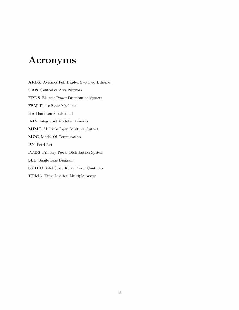
AFDX Avionics Full Duplex Switched Ethernet
CAN Controller Area Network
EPDS Electric Power Distribution System
FSM Finite State Machine
HS Hamilton Sundstrand
IMA Integrated Modular Avionics
MIMO Multiple Input Multiple Output
MOC Model Of Computation
PN Petri Net
PPDS Primary Power Distribution System
SLD Single Line Diagram
SSRPC Solid State Relay Power Contactor
TDMA Time Division Multiple Access
8

Chapter 1
Introduction
1.1 Background
Modern aircraft rely on the integration of several systems such as the Electrical System, the Air ManagementSystem, Avionics, Vehicle Management and others. Most recent aircraft have seen a drive towards increasedintegration and more reliance on system control to achieve system functionality. Most control systems areimplemented using a combination of hardware and software systems and are designed to work under normaland fault conditions to ensure system performance and availability.
The control system often is distributed across several computational nodes and using communicationnetworks to exchange data in real-time. In the past this was often done using point-to-point communicationnetworks, however recent platforms have started to shift towards high speed bus based architectures. De-veloping control algorithms for these systems is particularly challenging due to the need for fault handlingand degraded performance requirements. It is therefore desirable to have a methodology (and supportingmodeling framework) that allows for the designer to approach the design in a modular fashion, rather thana fully integrated approach from the start.
In addition, there is a need to predict the early impact of the embedded architecture on the controlperformance. The control performance in such Integrated Modular Avionics (IMA) based systems often isimpacted by delay and jitter that are introduced by both the computational and communication elements.
To support both types of analysis, two existing toolsets will be evaluated for the application to currentand future aircraft systems. These two toolsets, JGrafchart and TrueTime have been developed at LundUniversity since 1991 and 1999 respectively.
The thesis has been done at UTC Aerospace Systems (legacy Hamilton Sundstrand) in Windsor Locks(CT, U.S ) which is a business division within the United Technologies Corporation (UTC). UTC consistsof six business divisions. The aerospace businesses are Sikorsky which is the largest helicopter manufacturerin the world, Pratt & Whitney which develops engines, industrial gas turbines and space propulsion systemsand UTC Aerospace systems. UTC Aerospace system is a major supplier to aerospace and defense systemsas well as to international space programs. The company is the result of the merging of Hamilton Sundstrandand Goodrich, which was completed in 2012. UTC also has commercial businesses which are Otis elevatorsand UTC Climate, Controls & Security.
1.2 Thesis Outline
This thesis aims to address two applications of control and analysis tools to support development of aircraftcontrol systems:
1. Investigate the applicability of JGrafchart and its associated Model of Computation (MoC) for de-scribing the Primary Power Distribution Control System.
2. Extension of the TrueTime toolbox to typical aircraft control systems that employ Integrated ModularAvionics (IMA).
10
1.3. RELATED WORK CHAPTER 1. INTRODUCTION
Within the first part a typical Electric Control System that forms the basis for the investigation of usingJGrafchart is described. A brief comparison of different Models of Computation (MoC) is detailed in Chapter3, and the application to Electric Systems is described in Chapter 4. Conclusions and future work for thispart is summarized in Chapter 5.
A similar outline is followed for the second part of this thesis. The IMA concept is described in Chapter 6,followed by a description of the TrueTime background in Chapter 7 and a Use Case and the implementationof the necessary extensions in Chapter 8. The thesis is concluded with Chapter 9 for the second part of thethesis.
1.3 Related Work
Modeling of avionic systems has grown more difficult as system complexity has increased significantly overthe past years. It becomes more and more important to construct models designed for verification, since thesesystems cannot be analyzed without the use of verification tools. Several large industry and governmentprograms have developed methods for both design and verification of complex aircraft systems. Withinthe More Open Electrical Technologies (MOET) [1] program new modeling methodologies focused on thefeasibility of more electric and integrated aircraft are investigated. In [2] the Modelica language is used as acommon language for modeling aircraft systems in the different domains. An example of related work in thearea of modeling and verification of avionic systems is provided in [3]. The authors propose an automatedprocedure for designing control protocols using Linear Temporal Logic to correctly describe the behavior ofa system and its environment. The motivation behind this is to make the model amenable to formal analysisand create a hierarchical control structure.
1.4 Individual Contributions
The work behind this thesis has been done in close collaboration between the authors, and both have beenworking with both parts. However, Sofia had the main responsibility for the JGrafchart part whereas Annahad the main responsibility for the TrueTime part. Since the scope of the JGrafchart part exceeds the scopeof the TrueTime part, Anna has also been responsible for the work done in Section 4.4.1.
11
Part I
Sequential Control Systems
12

Chapter 2
Primary Power Distribution Systems
2.1 Background
In today’s aircraft powering is done dynamically by the Electric Power Distribution Systems (EPDS). De-pending on which state the aircraft is in (take-off, landing etc) the routing will change accordingly by en-abling/disabling a set of switches. In the physical system redundant paths are available for the controller tochoose from. The controller has to choose a path and sequentialize the switches in a safe way, for example, ithas to guarantee no electric power loss in the system. To describe the behavior of the sequentialized systems,different Models of Computation can be used [5]. Among them are Finite State Machines (FSM) and PetriNets (PN), both of which have been used at Hamilton Sundstrand (HS) in the past for analysis purposes.The main objective of this part of the thesis is to model a PPDS control system in Simulink/JGrafchart andevaluate the expressiveness of the language, primarily to support fault handling.
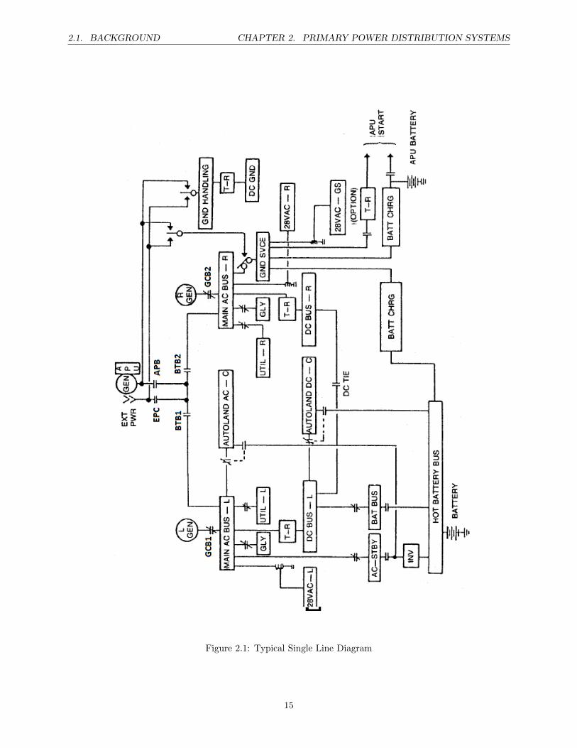
An Electric Power Distribution Systems (EPDS) is divided into Power generation, Protections and Pri-mary and Secondary power distribution, PPDS and SPDS respectively. The PPDS is responsible for protec-tions, input/output processing and supplying electric power to loads. The topology is shown in the singleline diagram (SLD), which can be seen in Figure 2.1.
The electric system consists of two sides, the left side and the right side. AC power is generated on eachside to power the AC loads. The AC power is converted to DC power to power the DC loads. The reasonfor using AC power is that it works at a higher voltage, which corresponds to a lower current. A low currentis preferred since it reduces losses such as power losses (proportional to current squared) as well as lowersthe weight since current conductors are heavy. As an added safety measure there is an independent systemin the middle, which in case of major failure provides power to the most critical loads in the system.
Listed below is a description of all sources and components shown in the SLD.
2.1.1 Sources
Left/Right Generator Since safety requirements on aircraft systems are rigid, redundancy in avionicssystems is necessary to guarantee sufficient power supply. Therefore, two main generators are placed oneach side of the aircraft. Under normal circumstances the generators power one side each, but depending onsource availability one generator could power the entire system by itself. The generators are connected totwo different main AC buses, from which power is distributed to the rest of the system [5].
Auxiliary Power Unit (APU) The APU is a gas turbine which primary function is to start the mainengines. In case both the left and right generator break, the APU can be used to provide backup electricityto the system [5].
External Power (EP) As the name suggest, EP means providing the system with electricity from anexternal source. The difference between EP and the other sources is that EP can only be used while theairplane is on ground since electricity is supplied through a ground cart [5].
14
2.1. BACKGROUND CHAPTER 2. PRIMARY POWER DISTRIBUTION SYSTEMS
Figure 2.1: Typical Single Line Diagram
15
2.1. BACKGROUND CHAPTER 2. PRIMARY POWER DISTRIBUTION SYSTEMS
Figure 2.2: Priority Table
Ram Air Turbine (RAT) As one of the final protections the RAT exists to prevent power outage inthe system and provide power to the hydraulics and electrical system. The RAT is used when most of allother power sources has broken down or are unavailable. It is an air-driven turbine connected to a smallemergency generator. For a short period of time, the RAT is able to provide power to the most critical partsof the system and the most important flight instruments [5].
Batteries The batteries provide storage for electric power independent of the generators. They are usedin system startup or emergency situations. In case of emergency, they supply short term powering (up to 30minutes) while other sources are being prepared to take over [5].
2.1.2 Electrical Components
Transformer Rectifier Unit (TRU) A TRU is a conversion unit which transforms AC power to DCpower [5].
Contactors Contactors are devices that can be either open or closed. The state of the contactor indicateswhether electric power may pass through it or not. The configuration of the contactors determines therouting of electric power in the system. A contactor has several failure modes, two of them are the FailedTo Close (FTC) and Failed To Open (FTO) state. A contactor is determined to be in failure mode if it doesnot respond to a command within a certain amount of time [5].
Buses The electrical buses distribute power to the loads in the system [5].
2.1.3 Control Algorithm
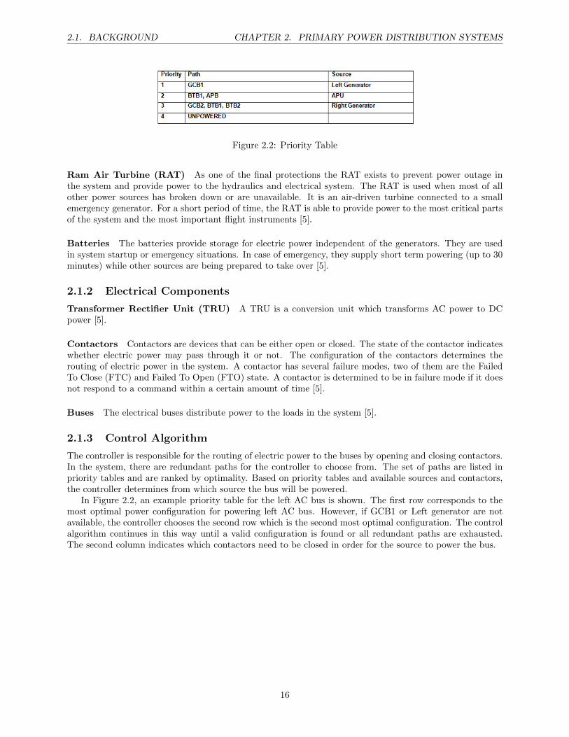
The controller is responsible for the routing of electric power to the buses by opening and closing contactors.In the system, there are redundant paths for the controller to choose from. The set of paths are listed inpriority tables and are ranked by optimality. Based on priority tables and available sources and contactors,the controller determines from which source the bus will be powered.
In Figure 2.2, an example priority table for the left AC bus is shown. The first row corresponds to themost optimal power configuration for powering left AC bus. However, if GCB1 or Left generator are notavailable, the controller chooses the second row which is the second most optimal configuration. The controlalgorithm continues in this way until a valid configuration is found or all redundant paths are exhausted.The second column indicates which contactors need to be closed in order for the source to power the bus.
16

Chapter 3
Models of Computation for SequentialControl Systems
A model of computation is a formal, abstract description of a system and its behavior, showing how thepieces in it relate to each other. The gain of describing a system formally is that it can then be transformedinto an analyzable format which makes it amenable to analysis using standard methods. The sections in thischapter describe different MoCs and modeling tool for sequential logic.
3.1 Finite State Machine
A finite state machine is a mathematical model used to describe an event-driven system. It consists of a finitenumber of states and a set of triggering conditions which cause the system to change state. The triggeringconditions are called events. A finite state machine is often summarized in a transition table, which specifiesthe input and output for each transition. The output from a FSM may differ depending on what type ofFSM is used, a Moore machine or a Mealy machine. These are described in short below [6].
3.1.1 Moore Machine
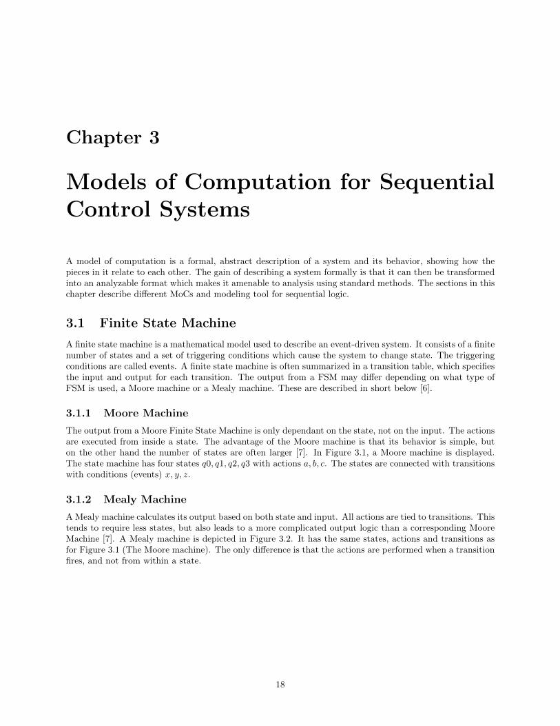
The output from a Moore Finite State Machine is only dependant on the state, not on the input. The actionsare executed from inside a state. The advantage of the Moore machine is that its behavior is simple, buton the other hand the number of states are often larger [7]. In Figure 3.1, a Moore machine is displayed.The state machine has four states q0, q1, q2, q3 with actions a, b, c. The states are connected with transitionswith conditions (events) x, y, z.
3.1.2 Mealy Machine
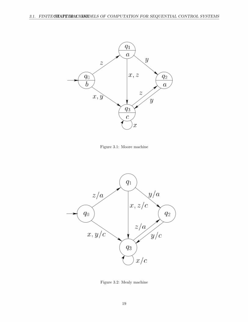
A Mealy machine calculates its output based on both state and input. All actions are tied to transitions. Thistends to require less states, but also leads to a more complicated output logic than a corresponding MooreMachine [7]. A Mealy machine is depicted in Figure 3.2. It has the same states, actions and transitions asfor Figure 3.1 (The Moore machine). The only difference is that the actions are performed when a transitionfires, and not from within a state.
18
3.1. FINITE STATE MACHINECHAPTER 3. MODELS OF COMPUTATION FOR SEQUENTIAL CONTROL SYSTEMS
Figure 3.1: Moore machine
Figure 3.2: Mealy machine
19
3.2. PETRI NETCHAPTER 3. MODELS OF COMPUTATION FOR SEQUENTIAL CONTROL SYSTEMS
3.2 Petri Net
3.2.1 Background
A Petri net is a mathematical and graphical modeling tool which can be used to model systems of concurrent,sequential, asynchronous, distributed, nondeterministic and/or stochastic character [9].
A Petri net is a bipartite directed graph, made up by three main components; places, transitions andarcs. A Bipartite graph is a graph where the nodes (places and transitions for this case) can be divided intotwo separate subsets such that each arc connects a node from one subset to a node in the other subset. Ifthe arcs are directed it is called a bipartite directed graph [10].
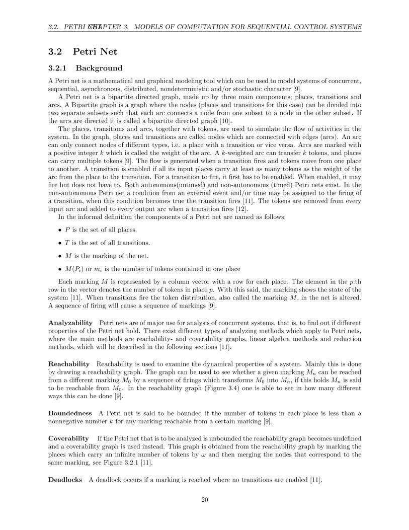
The places, transitions and arcs, together with tokens, are used to simulate the flow of activities in thesystem. In the graph, places and transitions are called nodes which are connected with edges (arcs). An arccan only connect nodes of different types, i.e. a place with a transition or vice versa. Arcs are marked witha positive integer k which is called the weight of the arc. A k-weighted arc can transfer k tokens, and placescan carry multiple tokens [9]. The flow is generated when a transition fires and tokens move from one placeto another. A transition is enabled if all its input places carry at least as many tokens as the weight of thearc from the place to the transition. For a transition to fire, it first has to be enabled. When enabled, it mayfire but does not have to. Both autonomous(untimed) and non-autonomous (timed) Petri nets exist. In thenon-autonomous Petri net a condition from an external event and/or time may be assigned to the firing ofa transition, when this condition becomes true the transition fires [11]. The tokens are removed from everyinput arc and added to every output arc when a transition fires [12].
In the informal definition the components of a Petri net are named as follows:
• P is the set of all places.
• T is the set of all transitions.
• M is the marking of the net.
• M(Pi) or mi is the number of tokens contained in one place
Each marking M is represented by a column vector with a row for each place. The element in the p:throw in the vector denotes the number of tokens in place p. With this said, the marking shows the state of thesystem [11]. When transitions fire the token distribution, also called the marking M , in the net is altered.A sequence of firing will cause a sequence of markings [9].
Analyzability Petri nets are of major use for analysis of concurrent systems, that is, to find out if differentproperties of the Petri net hold. There exist different types of analyzing methods which apply to Petri nets,where the main methods are reachability- and coverability graphs, linear algebra methods and reductionmethods, which will be described in the following sections [11].
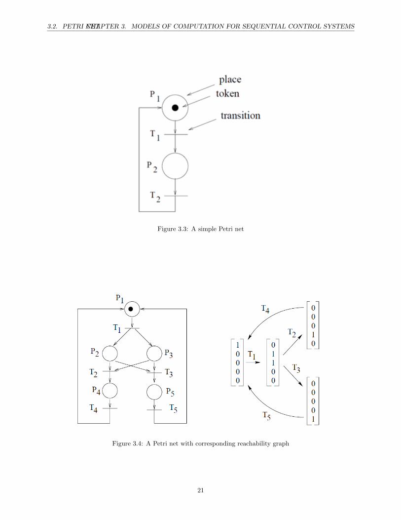
Reachability Reachability is used to examine the dynamical properties of a system. Mainly this is doneby drawing a reachability graph. The graph can be used to see whether a given marking Mn can be reachedfrom a different marking M0 by a sequence of firings which transforms M0 into Mn, if this holds Mn is saidto be reachable from M0. In the reachability graph (Figure 3.4) one is able to see in how many differentways this can be done [9].
Boundedness A Petri net is said to be bounded if the number of tokens in each place is less than anonnegative number k for any marking reachable from a certain marking [9].
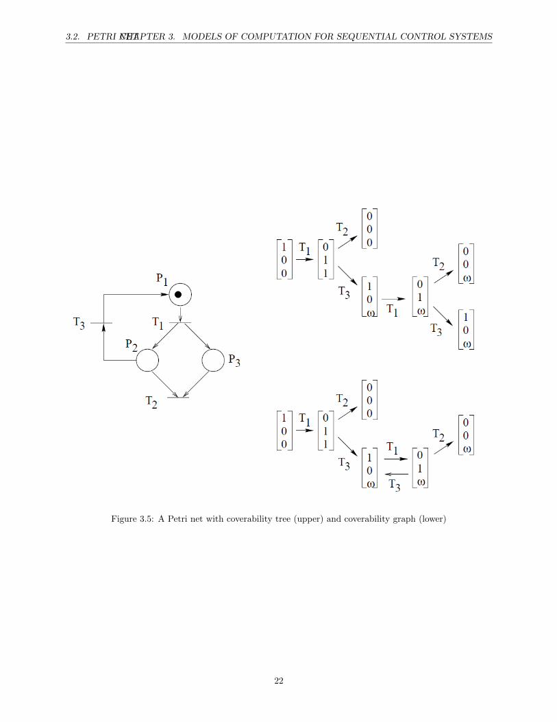
Coverability If the Petri net that is to be analyzed is unbounded the reachability graph becomes undefinedand a coverability graph is used instead. This graph is obtained from the reachability graph by marking theplaces which carry an infinite number of tokens by ω and then merging the nodes that correspond to thesame marking, see Figure 3.2.1 [11].
Deadlocks A deadlock occurs if a marking is reached where no transitions are enabled [11].
20
3.2. PETRI NETCHAPTER 3. MODELS OF COMPUTATION FOR SEQUENTIAL CONTROL SYSTEMS
Figure 3.3: A simple Petri net
Figure 3.4: A Petri net with corresponding reachability graph
21
3.2. PETRI NETCHAPTER 3. MODELS OF COMPUTATION FOR SEQUENTIAL CONTROL SYSTEMS
Figure 3.5: A Petri net with coverability tree (upper) and coverability graph (lower)
22
3.3. DIFFERENT TYPES OF PETRI NETSCHAPTER 3. MODELS OF COMPUTATION FOR SEQUENTIAL CONTROL SYSTEMS
Linear algebra The properties of a Petri net can be determined by the use of mathematical methods inorder to find out about the invariants of the net. If no deadlocks exist there will be an infinite number offirings, however this is most often not the case, all markings cannot be reached and not all sequences of firingcan be done. This kind of restrictions is represented by the invariants of the net[11].
Reduction methods The reachability and coverability graphs are good analysis methods for small Petrinets, however they are not applicable to large systems. Therefore system models are often reduced to simplerones. There exist a lot of techniques which reduce large Petri nets into smaller ones without altering theproperties of the original net[11].
3.3 Different types of Petri nets
There exist both Petri nets and high-level Petri nets. The main and more informal difference between thetwo is that in the high-level Petri net different tokens can be distinguished and calculated with, which theycannot be in Petri nets. The following two paragraphs give an overview of two important high-level Petrinets; the colored Petri net and the object Petri net.
3.3.1 Colored Petri nets
The colored Petri net is a high-level petri net developed during the 1980s. The main idea is to assign eachtoken a color, which serves as an identifier for that token. Any Petri net can be transformed into a coloredPetri net, an action which makes them more compact in structure and easier to read and comprehend.
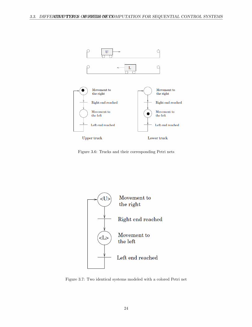
A simple example can be used to illustrate the benefits with colored Petri nets. Figure 3.6 describes twosystems that are identical, except for the direction in which the trucks are moving, and their correspondingPetri nets. In this arrangement the system is modeled with separate nets each containing one token. Thesystem could also be modeled with a colored Petri net. The Petri net would have two tokens whose label (orcolor) would mark the direction, see Fig 3.7. It is possible to transform a colored Petri net into a standardPetri net. This allows for analysis using the standard methods[11].
3.3.2 Object Petri nets
The concept of object Petri nets are inspired by high-level object-oriented programming languages, althoughonly two classes exist; one for tokens and one for modules/subnets. The main idea is to give the token itselfa Petri net structure which results in a net within a net structure. The layered approach is better suited formodeling of real system since they are not often ”flat”, but have internal structures that are of interest forthe modeler[13].
23
3.3. DIFFERENT TYPES OF PETRI NETSCHAPTER 3. MODELS OF COMPUTATION FOR SEQUENTIAL CONTROL SYSTEMS
Figure 3.6: Trucks and their corresponding Petri nets
Figure 3.7: Two identical systems modeled with a colored Petri net
24
3.4. STATEFLOWCHAPTER 3. MODELS OF COMPUTATION FOR SEQUENTIAL CONTROL SYSTEMS
3.4 Stateflow
Stateflow is an extension of Simulink, which supports sequential control through the use of flow diagramsand state charts. In Stateflow it is possible to have both Moore and Mealy FSM, which in combinationwith its integration with Simulink and Matlab makes it a powerful tool for modeling of sequential controlapplications. Stateflow also has built-in C-code generation.
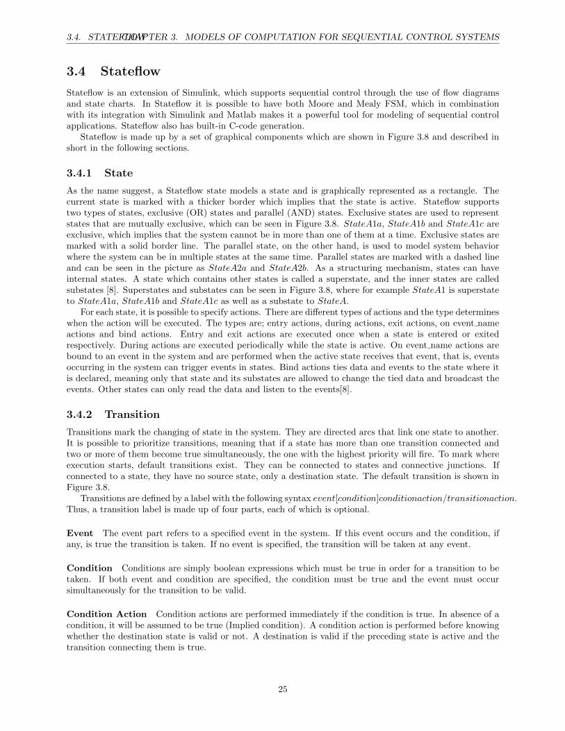
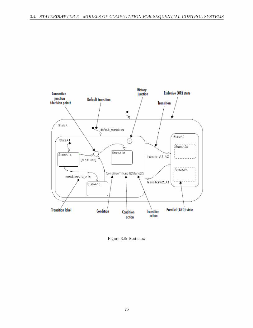
Stateflow is made up by a set of graphical components which are shown in Figure 3.8 and described inshort in the following sections.
3.4.1 State
As the name suggest, a Stateflow state models a state and is graphically represented as a rectangle. Thecurrent state is marked with a thicker border which implies that the state is active. Stateflow supportstwo types of states, exclusive (OR) states and parallel (AND) states. Exclusive states are used to representstates that are mutually exclusive, which can be seen in Figure 3.8. StateA1a, StateA1b and StateA1c areexclusive, which implies that the system cannot be in more than one of them at a time. Exclusive states aremarked with a solid border line. The parallel state, on the other hand, is used to model system behaviorwhere the system can be in multiple states at the same time. Parallel states are marked with a dashed lineand can be seen in the picture as StateA2a and StateA2b. As a structuring mechanism, states can haveinternal states. A state which contains other states is called a superstate, and the inner states are calledsubstates [8]. Superstates and substates can be seen in Figure 3.8, where for example StateA1 is superstateto StateA1a, StateA1b and StateA1c as well as a substate to StateA.
For each state, it is possible to specify actions. There are different types of actions and the type determineswhen the action will be executed. The types are; entry actions, during actions, exit actions, on event nameactions and bind actions. Entry and exit actions are executed once when a state is entered or exitedrespectively. During actions are executed periodically while the state is active. On event name actions arebound to an event in the system and are performed when the active state receives that event, that is, eventsoccurring in the system can trigger events in states. Bind actions ties data and events to the state where itis declared, meaning only that state and its substates are allowed to change the tied data and broadcast theevents. Other states can only read the data and listen to the events[8].
3.4.2 Transition
Transitions mark the changing of state in the system. They are directed arcs that link one state to another.It is possible to prioritize transitions, meaning that if a state has more than one transition connected andtwo or more of them become true simultaneously, the one with the highest priority will fire. To mark whereexecution starts, default transitions exist. They can be connected to states and connective junctions. Ifconnected to a state, they have no source state, only a destination state. The default transition is shown inFigure 3.8.
Transitions are defined by a label with the following syntax event[condition]conditionaction/transitionaction.Thus, a transition label is made up of four parts, each of which is optional.
Event The event part refers to a specified event in the system. If this event occurs and the condition, ifany, is true the transition is taken. If no event is specified, the transition will be taken at any event.
Condition Conditions are simply boolean expressions which must be true in order for a transition to betaken. If both event and condition are specified, the condition must be true and the event must occursimultaneously for the transition to be valid.
Condition Action Condition actions are performed immediately if the condition is true. In absence of acondition, it will be assumed to be true (Implied condition). A condition action is performed before knowingwhether the destination state is valid or not. A destination is valid if the preceding state is active and thetransition connecting them is true.
25
3.4. STATEFLOWCHAPTER 3. MODELS OF COMPUTATION FOR SEQUENTIAL CONTROL SYSTEMS
Figure 3.8: Stateflow
26
3.5. GRAFCETCHAPTER 3. MODELS OF COMPUTATION FOR SEQUENTIAL CONTROL SYSTEMS
Figure 3.9: State machine without connective junction (Left) and state machine with connective junction(Right)
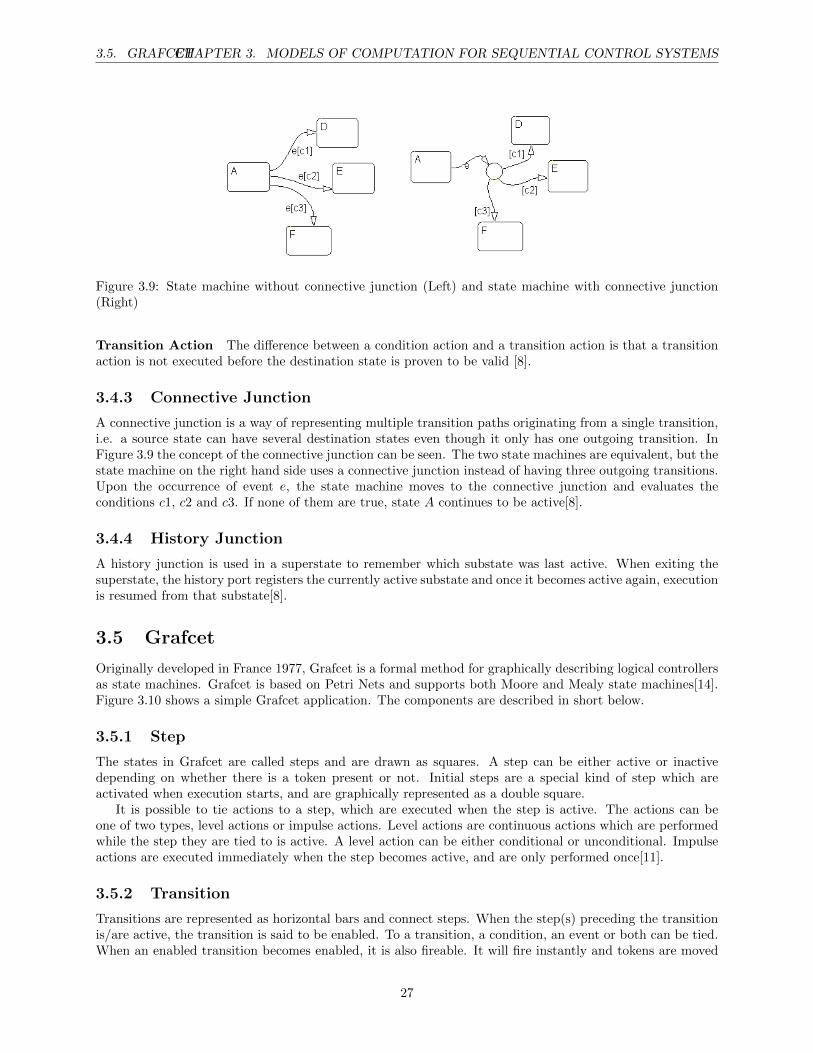
Transition Action The difference between a condition action and a transition action is that a transitionaction is not executed before the destination state is proven to be valid [8].
3.4.3 Connective Junction
A connective junction is a way of representing multiple transition paths originating from a single transition,i.e. a source state can have several destination states even though it only has one outgoing transition. InFigure 3.9 the concept of the connective junction can be seen. The two state machines are equivalent, but thestate machine on the right hand side uses a connective junction instead of having three outgoing transitions.Upon the occurrence of event e, the state machine moves to the connective junction and evaluates theconditions c1, c2 and c3. If none of them are true, state A continues to be active[8].
3.4.4 History Junction
A history junction is used in a superstate to remember which substate was last active. When exiting thesuperstate, the history port registers the currently active substate and once it becomes active again, executionis resumed from that substate[8].
3.5 Grafcet
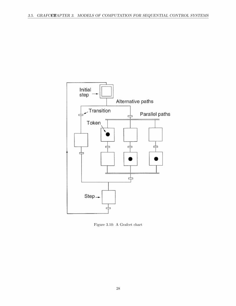
Originally developed in France 1977, Grafcet is a formal method for graphically describing logical controllersas state machines. Grafcet is based on Petri Nets and supports both Moore and Mealy state machines[14].Figure 3.10 shows a simple Grafcet application. The components are described in short below.
3.5.1 Step
The states in Grafcet are called steps and are drawn as squares. A step can be either active or inactivedepending on whether there is a token present or not. Initial steps are a special kind of step which areactivated when execution starts, and are graphically represented as a double square.
It is possible to tie actions to a step, which are executed when the step is active. The actions can beone of two types, level actions or impulse actions. Level actions are continuous actions which are performedwhile the step they are tied to is active. A level action can be either conditional or unconditional. Impulseactions are executed immediately when the step becomes active, and are only performed once[11].
3.5.2 Transition
Transitions are represented as horizontal bars and connect steps. When the step(s) preceding the transitionis/are active, the transition is said to be enabled. To a transition, a condition, an event or both can be tied.When an enabled transition becomes enabled, it is also fireable. It will fire instantly and tokens are moved
27
3.5. GRAFCETCHAPTER 3. MODELS OF COMPUTATION FOR SEQUENTIAL CONTROL SYSTEMS
Figure 3.10: A Grafcet chart
28
3.6. SEQUENTIAL FUNCTION CHARTSCHAPTER 3. MODELS OF COMPUTATION FOR SEQUENTIAL CONTROL SYSTEMS
Figure 3.11: Grafcet Macro Step
to the succeeding step(s). In Grafcet, there is no support for prioritizing transitions. If a step has morethan one outgoing transition and several of them are fireable at the same time, all fireable transitions willfire simultaneously. If, when a step is entered, its outgoing transition fires immediately the situation is saidto be unstable. In this case, only the impulse actions are performed[11].
3.5.3 Branching
In Grafcet, both alternative and parallel branches can be used. If an ingoing transition which connects morethan one step through the use of a parallel path fires, all steps succeeding it will become active. Furthermore,for outgoing transitions connected to more than one preceding step, all steps preceding the transition mustbe active for the transition to enable[11]. The concept of branching is visualized in Figure 3.10.
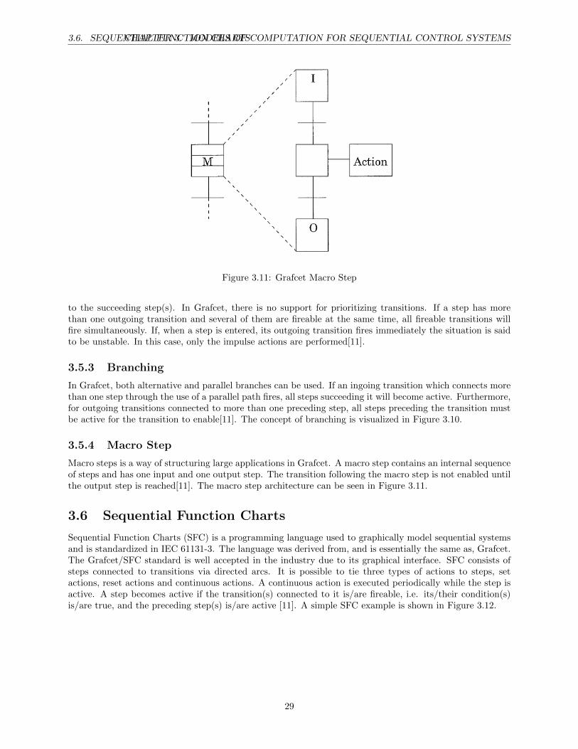
3.5.4 Macro Step
Macro steps is a way of structuring large applications in Grafcet. A macro step contains an internal sequenceof steps and has one input and one output step. The transition following the macro step is not enabled untilthe output step is reached[11]. The macro step architecture can be seen in Figure 3.11.
3.6 Sequential Function Charts
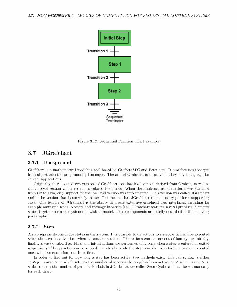
Sequential Function Charts (SFC) is a programming language used to graphically model sequential systemsand is standardized in IEC 61131-3. The language was derived from, and is essentially the same as, Grafcet.The Grafcet/SFC standard is well accepted in the industry due to its graphical interface. SFC consists ofsteps connected to transitions via directed arcs. It is possible to tie three types of actions to steps, setactions, reset actions and continuous actions. A continuous action is executed periodically while the step isactive. A step becomes active if the transition(s) connected to it is/are fireable, i.e. its/their condition(s)is/are true, and the preceding step(s) is/are active [11]. A simple SFC example is shown in Figure 3.12.
29
3.7. JGRAFCHARTCHAPTER 3. MODELS OF COMPUTATION FOR SEQUENTIAL CONTROL SYSTEMS
Figure 3.12: Sequential Function Chart example
3.7 JGrafchart
3.7.1 Background
Grafchart is a mathematical modeling tool based on Grafcet/SFC and Petri nets. It also features conceptsfrom object-oriented programming languages. The aim of Grafchart is to provide a high-level language forcontrol applications.
Originally there existed two versions of Grafchart, one low level version derived from Grafcet, as well asa high level version which resembles colored Petri nets. When the implementation platform was switchedfrom G2 to Java, only support for the low level version was implemented. This version was called JGrafchartand is the version that is currently in use. This means that JGrafchart runs on every platform supportingJava. One feature of JGrafchart is the ability to create extensive graphical user interfaces, including forexample animated icons, plotters and message browsers [15]. JGrafchart features several graphical elementswhich together form the system one wish to model. These components are briefly described in the followingparagraphs.
3.7.2 Step
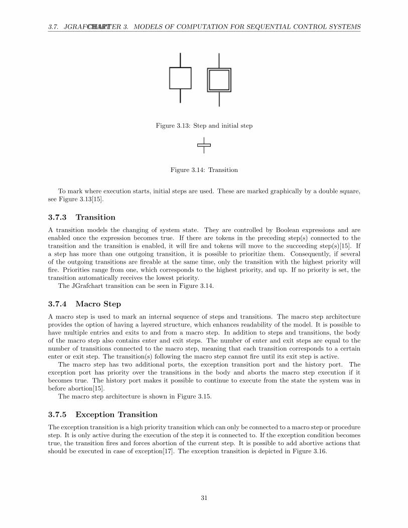
A step represents one of the states in the system. It is possible to tie actions to a step, which will be executedwhen the step is active, i.e. when it contains a token. The actions can be one out of four types; initially,finally, always or abortive. Final and initial actions are performed only once when a step is entered or exitedrespectively. Always actions are executed periodically while the step is active. Abortive actions are executedonce when an exception transition fires.
In order to find out for how long a step has been active, two methods exist. The call syntax is either< step− name > .s, which returns the number of seconds the step has been active, or < step− name > .t,which returns the number of periods. Periods in JGrafchart are called Scan Cycles and can be set manuallyfor each chart.
30
3.7. JGRAFCHARTCHAPTER 3. MODELS OF COMPUTATION FOR SEQUENTIAL CONTROL SYSTEMS
Figure 3.13: Step and initial step
Figure 3.14: Transition
To mark where execution starts, initial steps are used. These are marked graphically by a double square,see Figure 3.13[15].
3.7.3 Transition
A transition models the changing of system state. They are controlled by Boolean expressions and areenabled once the expression becomes true. If there are tokens in the preceding step(s) connected to thetransition and the transition is enabled, it will fire and tokens will move to the succeeding step(s)[15]. Ifa step has more than one outgoing transition, it is possible to prioritize them. Consequently, if severalof the outgoing transitions are fireable at the same time, only the transition with the highest priority willfire. Priorities range from one, which corresponds to the highest priority, and up. If no priority is set, thetransition automatically receives the lowest priority.
The JGrafchart transition can be seen in Figure 3.14.
3.7.4 Macro Step
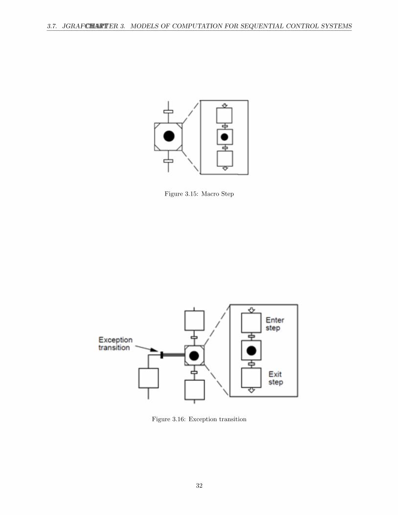
A macro step is used to mark an internal sequence of steps and transitions. The macro step architectureprovides the option of having a layered structure, which enhances readability of the model. It is possible tohave multiple entries and exits to and from a macro step. In addition to steps and transitions, the bodyof the macro step also contains enter and exit steps. The number of enter and exit steps are equal to thenumber of transitions connected to the macro step, meaning that each transition corresponds to a certainenter or exit step. The transition(s) following the macro step cannot fire until its exit step is active.
The macro step has two additional ports, the exception transition port and the history port. Theexception port has priority over the transitions in the body and aborts the macro step execution if itbecomes true. The history port makes it possible to continue to execute from the state the system was inbefore abortion[15].
The macro step architecture is shown in Figure 3.15.
3.7.5 Exception Transition
The exception transition is a high priority transition which can only be connected to a macro step or procedurestep. It is only active during the execution of the step it is connected to. If the exception condition becomestrue, the transition fires and forces abortion of the current step. It is possible to add abortive actions thatshould be executed in case of exception[17]. The exception transition is depicted in Figure 3.16.
31
3.7. JGRAFCHARTCHAPTER 3. MODELS OF COMPUTATION FOR SEQUENTIAL CONTROL SYSTEMS
Figure 3.15: Macro Step
Figure 3.16: Exception transition
32
3.7. JGRAFCHARTCHAPTER 3. MODELS OF COMPUTATION FOR SEQUENTIAL CONTROL SYSTEMS
Figure 3.17: Procedure step
Figure 3.18: Process step
3.7.6 Procedure Step
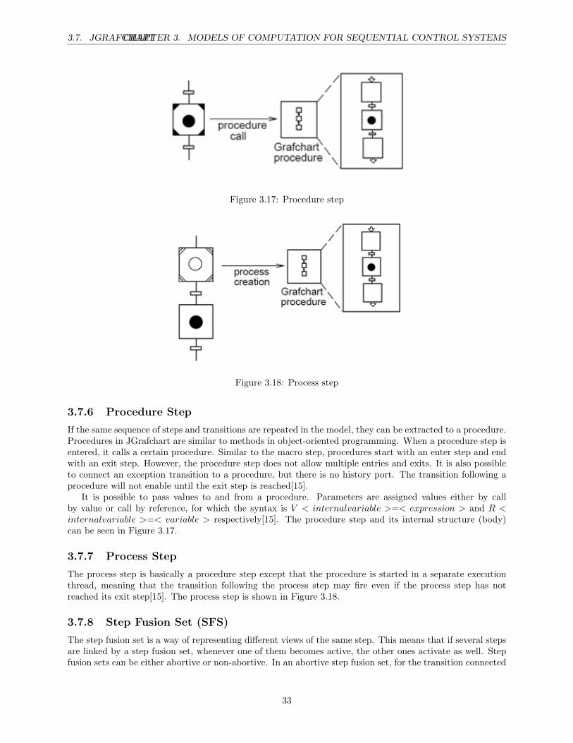
If the same sequence of steps and transitions are repeated in the model, they can be extracted to a procedure.Procedures in JGrafchart are similar to methods in object-oriented programming. When a procedure step isentered, it calls a certain procedure. Similar to the macro step, procedures start with an enter step and endwith an exit step. However, the procedure step does not allow multiple entries and exits. It is also possibleto connect an exception transition to a procedure, but there is no history port. The transition following aprocedure will not enable until the exit step is reached[15].
It is possible to pass values to and from a procedure. Parameters are assigned values either by callby value or call by reference, for which the syntax is V < internalvariable >=< expression > and R <internalvariable >=< variable > respectively[15]. The procedure step and its internal structure (body)can be seen in Figure 3.17.
3.7.7 Process Step
The process step is basically a procedure step except that the procedure is started in a separate executionthread, meaning that the transition following the process step may fire even if the process step has notreached its exit step[15]. The process step is shown in Figure 3.18.
3.7.8 Step Fusion Set (SFS)
The step fusion set is a way of representing different views of the same step. This means that if several stepsare linked by a step fusion set, whenever one of them becomes active, the other ones activate as well. Stepfusion sets can be either abortive or non-abortive. In an abortive step fusion set, for the transition connected
33
3.8. CHOOSING A MODEL OF COMPUTATIONCHAPTER 3. MODELS OF COMPUTATION FOR SEQUENTIAL CONTROL SYSTEMS
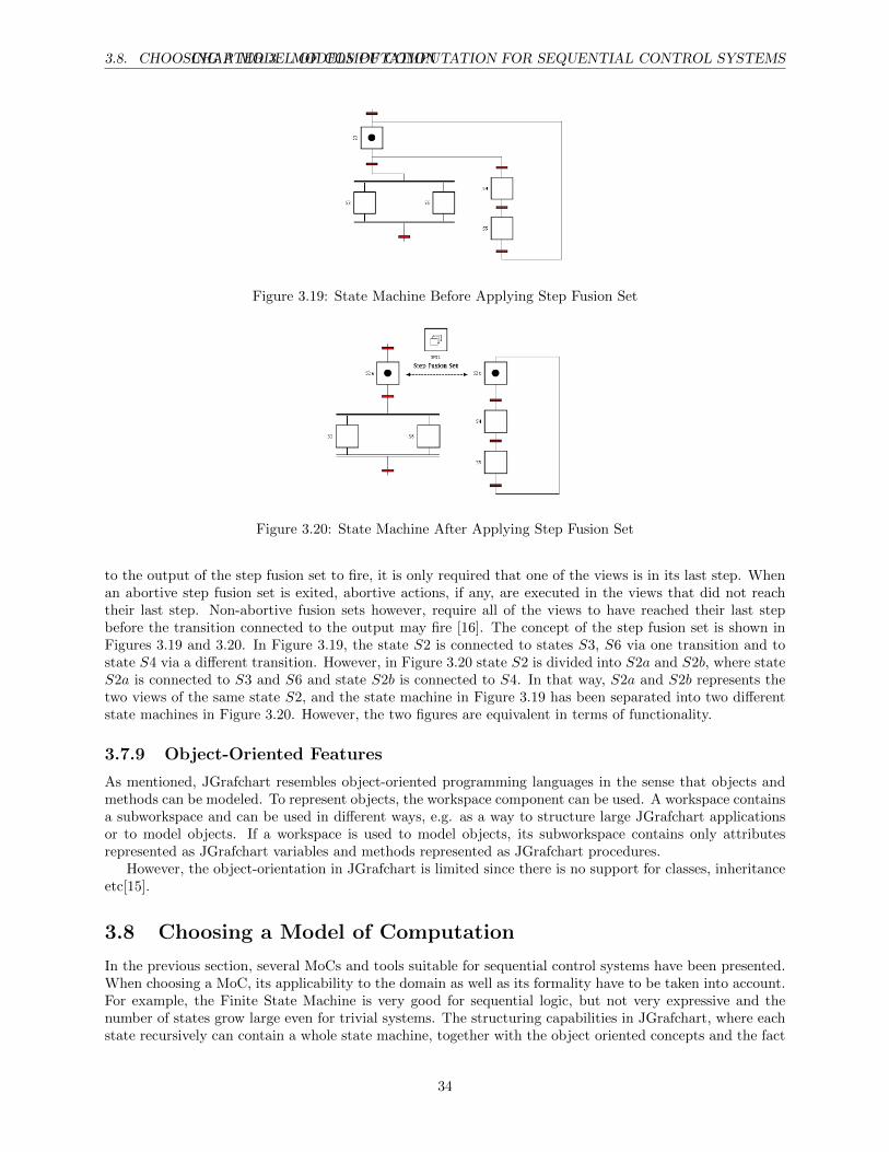
Figure 3.19: State Machine Before Applying Step Fusion Set
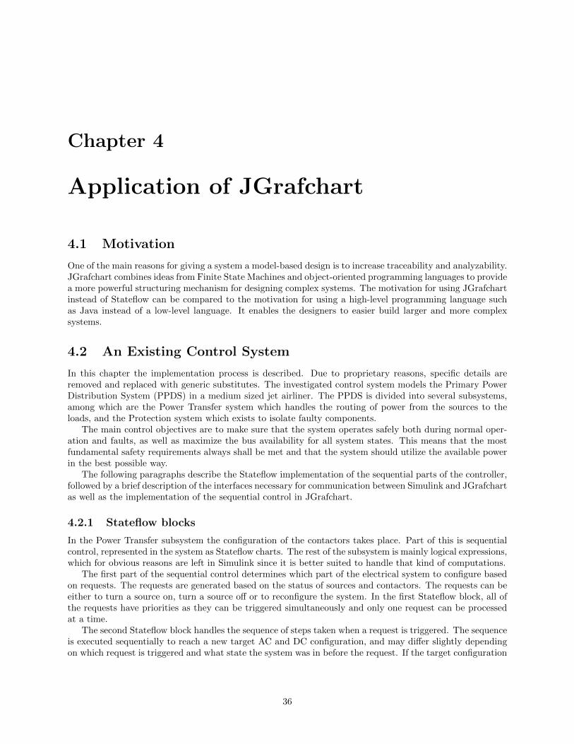
Figure 3.20: State Machine After Applying Step Fusion Set
to the output of the step fusion set to fire, it is only required that one of the views is in its last step. Whenan abortive step fusion set is exited, abortive actions, if any, are executed in the views that did not reachtheir last step. Non-abortive fusion sets however, require all of the views to have reached their last stepbefore the transition connected to the output may fire [16]. The concept of the step fusion set is shown inFigures 3.19 and 3.20. In Figure 3.19, the state S2 is connected to states S3, S6 via one transition and tostate S4 via a different transition. However, in Figure 3.20 state S2 is divided into S2a and S2b, where stateS2a is connected to S3 and S6 and state S2b is connected to S4. In that way, S2a and S2b represents thetwo views of the same state S2, and the state machine in Figure 3.19 has been separated into two differentstate machines in Figure 3.20. However, the two figures are equivalent in terms of functionality.
3.7.9 Object-Oriented Features
As mentioned, JGrafchart resembles object-oriented programming languages in the sense that objects andmethods can be modeled. To represent objects, the workspace component can be used. A workspace containsa subworkspace and can be used in different ways, e.g. as a way to structure large JGrafchart applicationsor to model objects. If a workspace is used to model objects, its subworkspace contains only attributesrepresented as JGrafchart variables and methods represented as JGrafchart procedures.
However, the object-orientation in JGrafchart is limited since there is no support for classes, inheritanceetc[15].
3.8 Choosing a Model of Computation
In the previous section, several MoCs and tools suitable for sequential control systems have been presented.When choosing a MoC, its applicability to the domain as well as its formality have to be taken into account.For example, the Finite State Machine is very good for sequential logic, but not very expressive and thenumber of states grow large even for trivial systems. The structuring capabilities in JGrafchart, where eachstate recursively can contain a whole state machine, together with the object oriented concepts and the fact
34

3.8. CHOOSING A MODEL OF COMPUTATIONCHAPTER 3. MODELS OF COMPUTATION FOR SEQUENTIAL CONTROL SYSTEMS
that it is transformable to a Petri net and can therefore be analyzed using standard methods makes it aninteresting tool to investigate.
35
Chapter 4
Application of JGrafchart
4.1 Motivation
One of the main reasons for giving a system a model-based design is to increase traceability and analyzability.JGrafchart combines ideas from Finite State Machines and object-oriented programming languages to providea more powerful structuring mechanism for designing complex systems. The motivation for using JGrafchartinstead of Stateflow can be compared to the motivation for using a high-level programming language suchas Java instead of a low-level language. It enables the designers to easier build larger and more complexsystems.
4.2 An Existing Control System
In this chapter the implementation process is described. Due to proprietary reasons, specific details areremoved and replaced with generic substitutes. The investigated control system models the Primary PowerDistribution System (PPDS) in a medium sized jet airliner. The PPDS is divided into several subsystems,among which are the Power Transfer system which handles the routing of power from the sources to theloads, and the Protection system which exists to isolate faulty components.
The main control objectives are to make sure that the system operates safely both during normal oper-ation and faults, as well as maximize the bus availability for all system states. This means that the mostfundamental safety requirements always shall be met and that the system should utilize the available powerin the best possible way.
The following paragraphs describe the Stateflow implementation of the sequential parts of the controller,followed by a brief description of the interfaces necessary for communication between Simulink and JGrafchartas well as the implementation of the sequential control in JGrafchart.
4.2.1 Stateflow blocks
In the Power Transfer subsystem the configuration of the contactors takes place. Part of this is sequentialcontrol, represented in the system as Stateflow charts. The rest of the subsystem is mainly logical expressions,which for obvious reasons are left in Simulink since it is better suited to handle that kind of computations.
The first part of the sequential control determines which part of the electrical system to configure basedon requests. The requests are generated based on the status of sources and contactors. The requests can beeither to turn a source on, turn a source off or to reconfigure the system. In the first Stateflow block, all ofthe requests have priorities as they can be triggered simultaneously and only one request can be processedat a time.
The second Stateflow block handles the sequence of steps taken when a request is triggered. The sequenceis executed sequentially to reach a new target AC and DC configuration, and may differ slightly dependingon which request is triggered and what state the system was in before the request. If the target configuration
36
4.3. JGRAFCHART CONTROL SYSTEM ARCHITECTURECHAPTER 4. APPLICATION OF JGRAFCHART
cannot be achieved due to unavailable contactors, the controller will re-execute the second Stateflow chartto find an alternative path.
4.2.2 Interfaces
Communicator between Simulink and JGrafchart
Since JGrafchart is not integrated with Simulink an interface had to be developed in order for them tocommunicate. This work was done at Lund University and resulted in a TCP/IP server allowing Simulinkand JGrafchart to exchange data over sockets. The server is placed in the Simulink model as a Simulinkblock. The server block receives and transmits messages using socket blocks in JGrafchart. The socketblocks in JGrafchart can be one of the following types; Real, Integer, Boolean or String. The format of themessage being sent starts with an identifier followed by the value. The identifier maps the Simulink signalsto the JGrafchart I/O Sockets, i.e. the signal name and the socket name must correspond.
The server has four arguments; InputPortMapping, OutputPortMapping, sampling time period and port.The InputPortMapping is a Simulink vector containing the identifiers for the input sockets in JGrafchart.If the size of the vector is larger than one, i.e. more than one signal is sent to JGrafchart, a multiplexerin Simulink is needed since the server only has one input port. The first element in the vector correspondsto the first port in the multiplexer, the second element to the second port and so on. This means that theorder of the identifiers are of significance. The same structure applies to the OutputPortMapping vector,except that a demultiplexer is used instead of a multiplexer at the output port on the server. The sampletime period is given in seconds and denotes how often the input signals to JGrafchart are read. The port isan integer indicating over which port communication takes place.
In addition to the server block, a block which controls the simulation time in Simulink was also im-plemented at Lund University. This was necessary since JGrafchart runs in real-time while Simulink runsin simulated time. The realtimer block synchronizes Simulink time with real time by slowing down thesimulated time periodically.
4.3 JGrafchart Control System Architecture
The first part of the implementation process focused only on the sequential control in the Stateflow blocks.The aim was to investigate whether an equivalent implementation in JGrafchart could be achieved, i.e.given the same input the Simulink state machines and the JGrafchart state machines would produce thesame output in terms of contactor configuration and, if any, lockouts.
The second part further extends the implementation by moving a larger part of the system from Simulinkto JGrafchart. A fault handling layer was implemented in JGrafchart to substitute the protection layer in theSimulink model. To detect faults, components in the system were modeled with individual state machines.This enables the controller to keep track of the state of each component in parallel with the control algorithm.If a fault occurs in any of the components, that state machine moves into a fault state which triggers thefault handling.
4.3.1 Sequential Control
Communication
As the name suggest, the communication layer handles the communication between Simulink and JGrafchart.This layer has no sequential control functionality but simply contains all the I/O sockets.
In the Simulink model, a fixed step size is used. The fixed step size puts constraints on the samplingtime in the sense that it must be a multiple of the fixed step size. In order for the model to executeproperly, the sampling time in the Simulink model must be the same as that in the server and realtimerblock. The sampling time indicates how often Simulink reads the server output port, meaning that if anoutput socket value in JGrafchart has changed more than once during one sample period, only the last changewill be registered by Simulink. To avoid this problem, some delay is introduced at concerned transitions inJGrafchart.
37
4.3. JGRAFCHART CONTROL SYSTEM ARCHITECTURECHAPTER 4. APPLICATION OF JGRAFCHART
Sequential Control
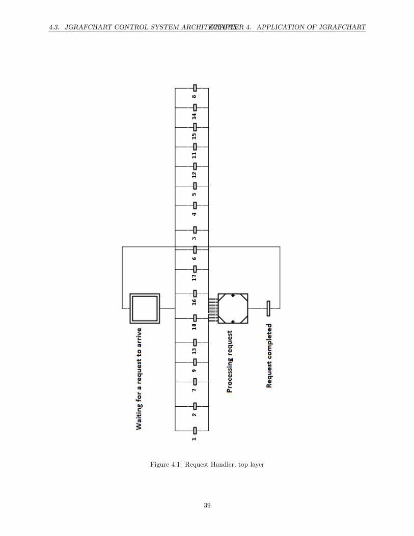
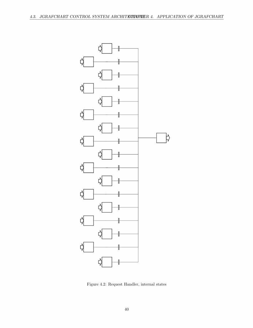
The JGrafchart model of the first Stateflow chart consists of two top level states, one state where the systemawaits requests and one where requests are processed. The second state has internal states, since thereare several different requests that may arrive. The layered structure introduced due to internal states isrepresented as a Multiple Input Multiple Output (MIMO) Macro step. The JGrafchart representation of thefirst Stateflow chart is shown in Figure 4.1 and 4.2.
Each transition in the top level corresponds to one request and listens to an input socket at the commu-nication layer, which represents its request. Since the Simulink model only processes one request at a time,the transitions between the two top level states are prioritized. When a transition at the top level fires atrigger is sent to the second sequential control block, which handles the sequence of steps taken to achievethe configuration needed to satisfy the request.
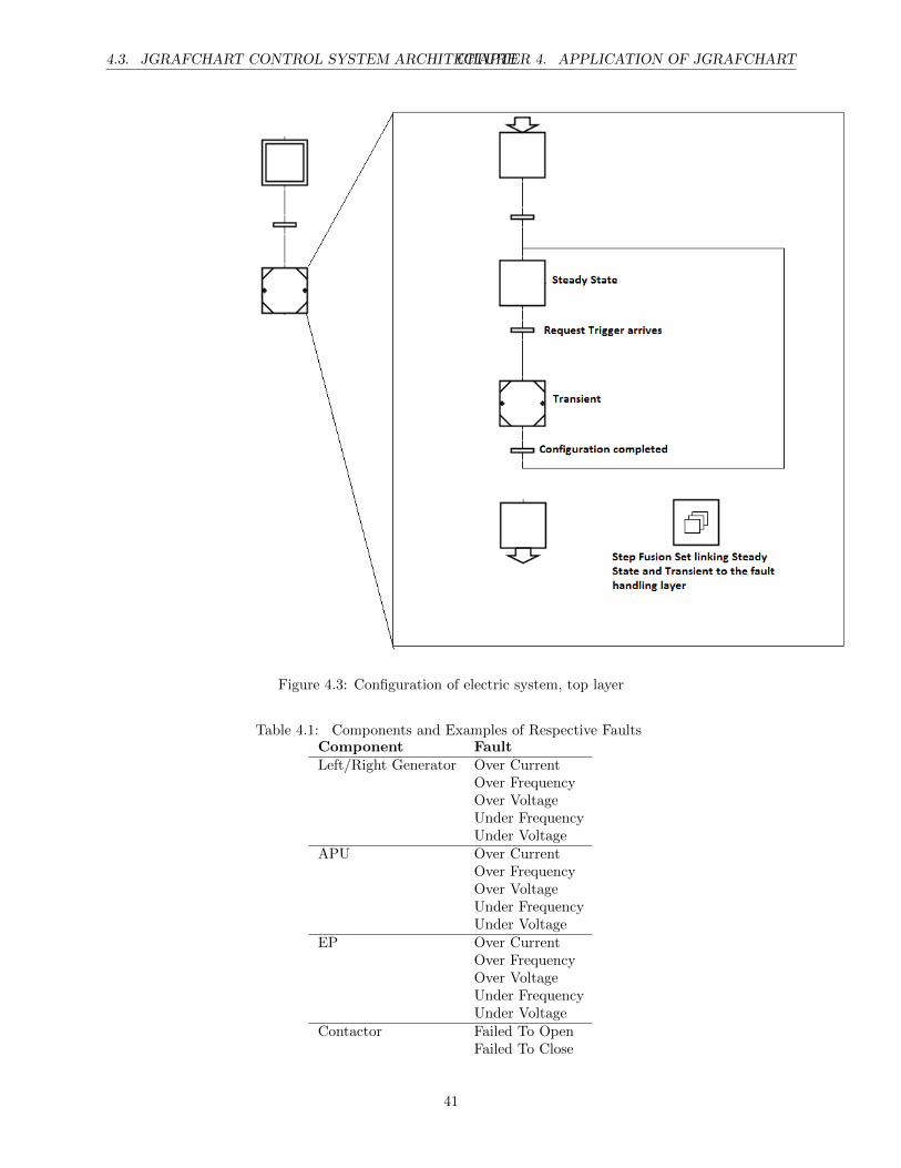
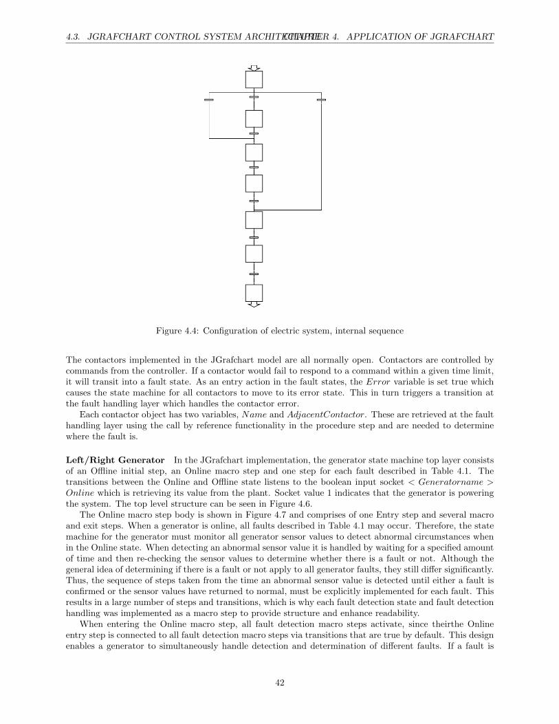
The highest level of abstraction when looking at the system as a whole are modeled by two states,one steady state and one transient state. When no requests are processed, the system is in steady stateand otherwise it is in transient, meaning that the electrical system is being configured. In the JGrafchartimplementation the steady state and transient state are placed in a macro step. The macro step in turn islinked to a detection step at a fault handling layer by an abortive step fusion set. Thus, error detection isprovided for all system states. Figure 4.3 and 4.4 show steady state and transient as well as the internalstates in transient. If an error occurs, the execution of the second part of the sequential control will beaborted. When the error has been resolved at the fault handling layer it will return to its detection stepand the sequential control will be re-activated and continue to execute from the state that was last active,according to the step fusion set logic. At the beginning of execution, the state machine is in steady state andremains there until triggered by the chart handling the requests. When the AC and DC target configurationsare reached, the state machine returns to its steady state and waits for the next trigger.
In order for the communication to work properly, delays are introduced at the transitions to make surethe input socket values are updated.
4.3.2 Sequential Control Integrated With Fault Handling
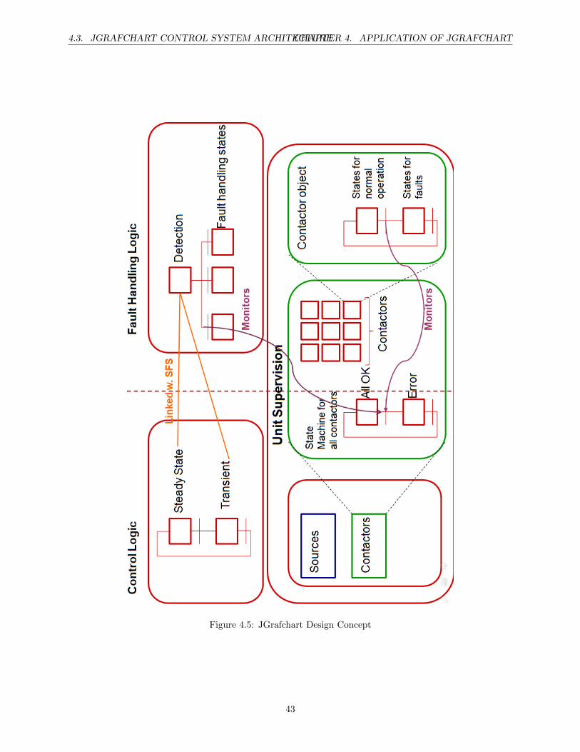
To determine whether there is a fault in the system, the state of each of its components is evaluated. Statemachines were implemented for each component to keep track of their current state. If an error occurs, thestate machine for the faulty component transits into an error state. The JGrafchart step fusion set featuremakes it possible to have a separate fault handling layer which monitors the component state machines inparallel with the execution of the control algorithm. Whenever a fault in a component is detected, a highpriority transition at the fault handling layer will fire and the exception actions will be performed. Differentcomponents experience different faults which are summarized in Table 4.1. Faults are of different severityand may inhibit requests as well as other fault handling. The design concept is shown in Figure 4.5.
As the aim of this thesis is to only investigate whether the MOC behind JGrafchart can be applied andprovide value to aircraft electric systems, only the components and their respective faults necessary to showa proof of concept were implemented.
Implementation of Components
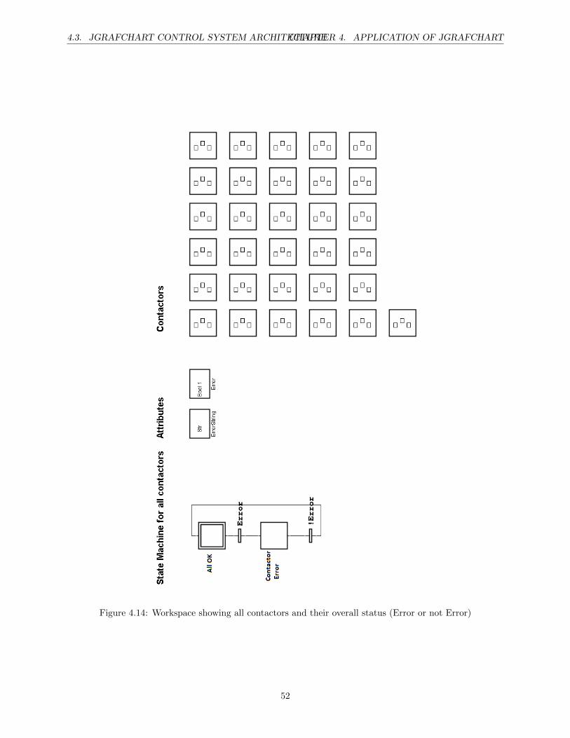
In JGrafchart, a component is modeled as an object through the use of a workspace. All workspaces containa state machine which models the behavior of the component. The transitions in the state machine listento input sockets at the Communication layer. The input are either data from the Plant indicating thecurrent state of the component or commands from the controller. Furthermore, components of the sametype (”instances of the same class”) are collected in a workspace together with a state machine showing ifthere is a fault in any of them. The state machine consists of two states, the initial state AllOK and theError state, which the state machine transits into whenever one of the components are in a faulty state.This structure can be seen in Figure 4.14.
The following paragraphs describe the components implemented in JGrafchart.
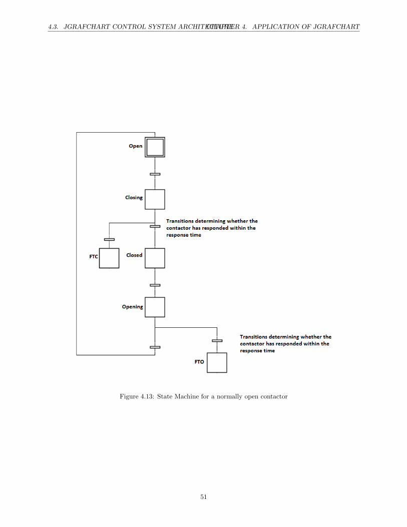
Contactor As an initial state, a contactor can be either open or closed denoted as normally open ornormally closed respectively. In Figure 4.13, the state machine for a normally open contactor is shown.
38
4.3. JGRAFCHART CONTROL SYSTEM ARCHITECTURECHAPTER 4. APPLICATION OF JGRAFCHART
Figure 4.1: Request Handler, top layer
39
4.3. JGRAFCHART CONTROL SYSTEM ARCHITECTURECHAPTER 4. APPLICATION OF JGRAFCHART
Figure 4.2: Request Handler, internal states
40
4.3. JGRAFCHART CONTROL SYSTEM ARCHITECTURECHAPTER 4. APPLICATION OF JGRAFCHART
Figure 4.3: Configuration of electric system, top layer
Table 4.1: Components and Examples of Respective FaultsComponent FaultLeft/Right Generator Over Current
Over FrequencyOver VoltageUnder FrequencyUnder Voltage
APU Over CurrentOver FrequencyOver VoltageUnder FrequencyUnder Voltage
EP Over CurrentOver FrequencyOver VoltageUnder FrequencyUnder Voltage
Contactor Failed To OpenFailed To Close
41
4.3. JGRAFCHART CONTROL SYSTEM ARCHITECTURECHAPTER 4. APPLICATION OF JGRAFCHART
Figure 4.4: Configuration of electric system, internal sequence
The contactors implemented in the JGrafchart model are all normally open. Contactors are controlled bycommands from the controller. If a contactor would fail to respond to a command within a given time limit,it will transit into a fault state. As an entry action in the fault states, the Error variable is set true whichcauses the state machine for all contactors to move to its error state. This in turn triggers a transition atthe fault handling layer which handles the contactor error.
Each contactor object has two variables, Name and AdjacentContactor. These are retrieved at the faulthandling layer using the call by reference functionality in the procedure step and are needed to determinewhere the fault is.
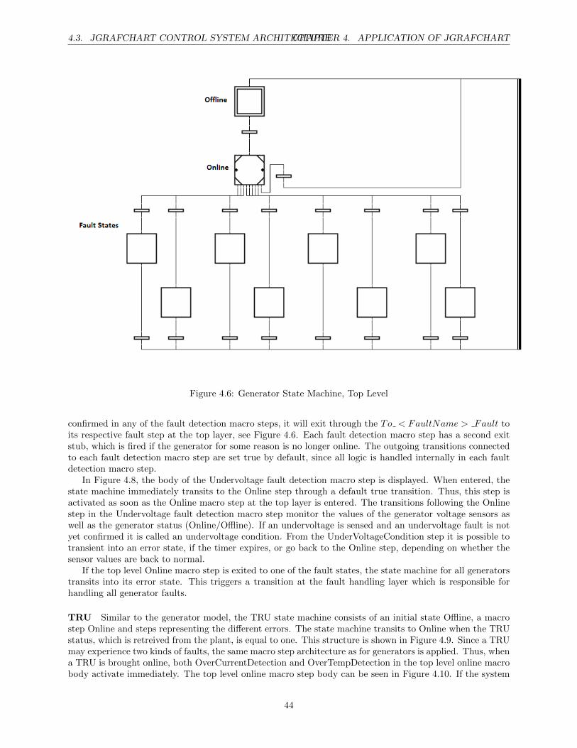
Left/Right Generator In the JGrafchart implementation, the generator state machine top layer consistsof an Offline initial step, an Online macro step and one step for each fault described in Table 4.1. Thetransitions between the Online and Offline state listens to the boolean input socket < Generatorname >Online which is retrieving its value from the plant. Socket value 1 indicates that the generator is poweringthe system. The top level structure can be seen in Figure 4.6.
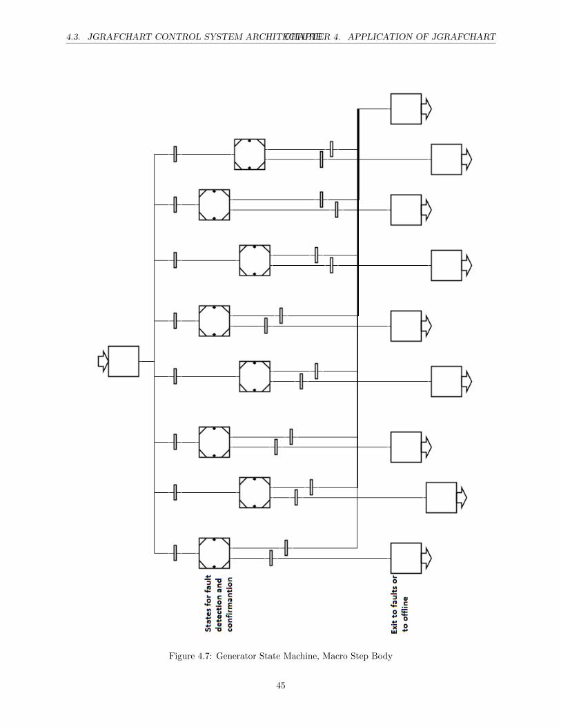
The Online macro step body is shown in Figure 4.7 and comprises of one Entry step and several macroand exit steps. When a generator is online, all faults described in Table 4.1 may occur. Therefore, the statemachine for the generator must monitor all generator sensor values to detect abnormal circumstances whenin the Online state. When detecting an abnormal sensor value it is handled by waiting for a specified amountof time and then re-checking the sensor values to determine whether there is a fault or not. Although thegeneral idea of determining if there is a fault or not apply to all generator faults, they still differ significantly.Thus, the sequence of steps taken from the time an abnormal sensor value is detected until either a fault isconfirmed or the sensor values have returned to normal, must be explicitly implemented for each fault. Thisresults in a large number of steps and transitions, which is why each fault detection state and fault detectionhandling was implemented as a macro step to provide structure and enhance readability.
When entering the Online macro step, all fault detection macro steps activate, since theirthe Onlineentry step is connected to all fault detection macro steps via transitions that are true by default. This designenables a generator to simultaneously handle detection and determination of different faults. If a fault is
42
4.3. JGRAFCHART CONTROL SYSTEM ARCHITECTURECHAPTER 4. APPLICATION OF JGRAFCHART
Figure 4.5: JGrafchart Design Concept
43
4.3. JGRAFCHART CONTROL SYSTEM ARCHITECTURECHAPTER 4. APPLICATION OF JGRAFCHART
Figure 4.6: Generator State Machine, Top Level
confirmed in any of the fault detection macro steps, it will exit through the To < FaultName > Fault toits respective fault step at the top layer, see Figure 4.6. Each fault detection macro step has a second exitstub, which is fired if the generator for some reason is no longer online. The outgoing transitions connectedto each fault detection macro step are set true by default, since all logic is handled internally in each faultdetection macro step.
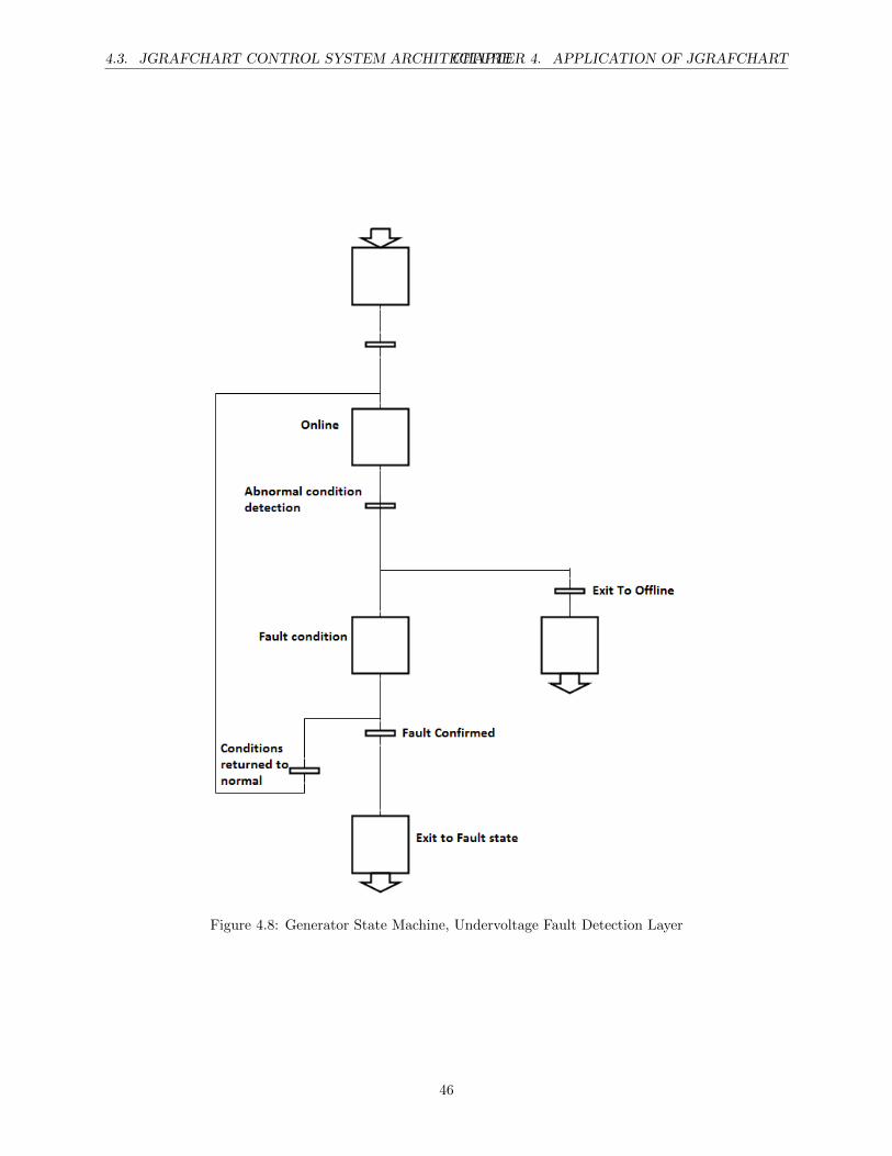
In Figure 4.8, the body of the Undervoltage fault detection macro step is displayed. When entered, thestate machine immediately transits to the Online step through a default true transition. Thus, this step isactivated as soon as the Online macro step at the top layer is entered. The transitions following the Onlinestep in the Undervoltage fault detection macro step monitor the values of the generator voltage sensors aswell as the generator status (Online/Offline). If an undervoltage is sensed and an undervoltage fault is notyet confirmed it is called an undervoltage condition. From the UnderVoltageCondition step it is possible totransient into an error state, if the timer expires, or go back to the Online step, depending on whether thesensor values are back to normal.
If the top level Online macro step is exited to one of the fault states, the state machine for all generatorstransits into its error state. This triggers a transition at the fault handling layer which is responsible forhandling all generator faults.
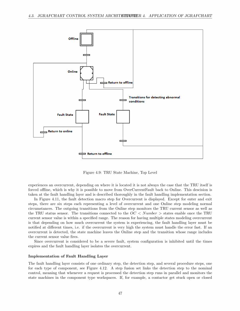
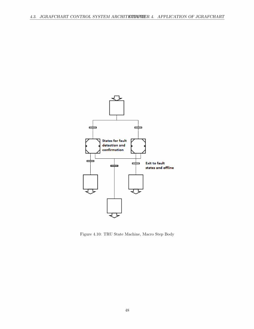
TRU Similar to the generator model, the TRU state machine consists of an initial state Offline, a macrostep Online and steps representing the different errors. The state machine transits to Online when the TRUstatus, which is retreived from the plant, is equal to one. This structure is shown in Figure 4.9. Since a TRUmay experience two kinds of faults, the same macro step architecture as for generators is applied. Thus, whena TRU is brought online, both OverCurrentDetection and OverTempDetection in the top level online macrobody activate immediately. The top level online macro step body can be seen in Figure 4.10. If the system
44
4.3. JGRAFCHART CONTROL SYSTEM ARCHITECTURECHAPTER 4. APPLICATION OF JGRAFCHART
Figure 4.7: Generator State Machine, Macro Step Body
45
4.3. JGRAFCHART CONTROL SYSTEM ARCHITECTURECHAPTER 4. APPLICATION OF JGRAFCHART
Figure 4.8: Generator State Machine, Undervoltage Fault Detection Layer
46
4.3. JGRAFCHART CONTROL SYSTEM ARCHITECTURECHAPTER 4. APPLICATION OF JGRAFCHART
Figure 4.9: TRU State Machine, Top Level
experiences an overcurrent, depending on where it is located it is not always the case that the TRU itself isforced offline, which is why it is possible to move from OverCurrentFault back to Online. This descision istaken at the fault handling layer and is described thoroughly in the fault handling implementation section.
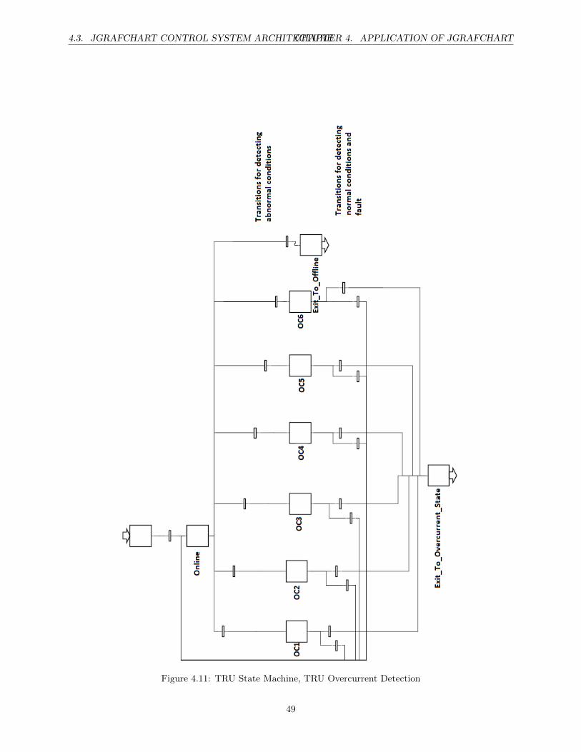
In Figure 4.11, the fault detection macro step for Overcurrent is displayed. Except for enter and exitsteps, there are six steps each representing a level of overcurrent and one Online step modeling normalcircumstances. The outgoing transitions from the Online step monitors the TRU current sensor as well asthe TRU status sensor. The transitions connected to the OC < Number > states enable once the TRUcurrent sensor value is within a specified range. The reason for having multiple states modeling overcurrentis that depending on how much overcurrent the system is experiencing, the fault handling layer must benotified at different times, i.e. if the overcurrent is very high the system must handle the error fast. If anovercurrent is detected, the state machine leaves the Online step and the transition whose range includesthe current sensor value fires.
Since overcurrent is considered to be a severe fault, system configuration is inhibited until the timesexpires and the fault handling layer isolates the overcurrent.
Implementation of Fault Handling Layer
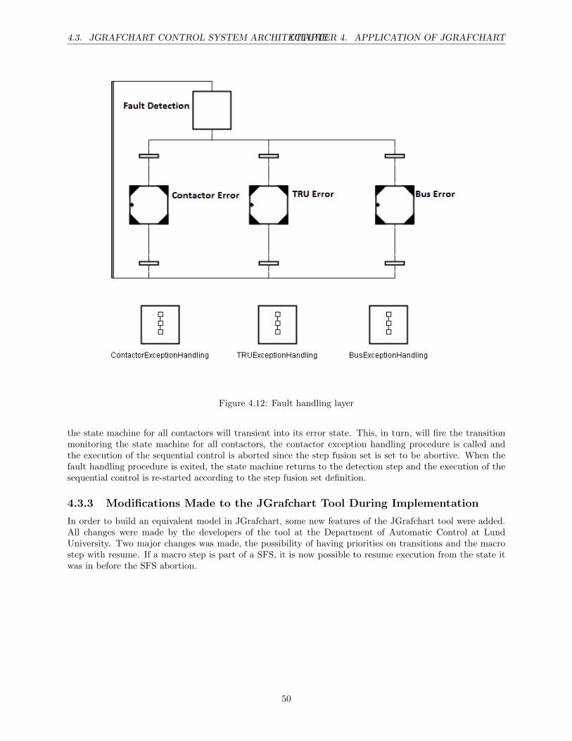
The fault handling layer consists of one ordinary step, the detection step, and several procedure steps, onefor each type of component, see Figure 4.12. A step fusion set links the detection step to the nominalcontrol, meaning that whenever a request is processed the detection step runs in parallel and monitors thestate machines in the component type workspaces. If, for example, a contactor get stuck open or closed
47
4.3. JGRAFCHART CONTROL SYSTEM ARCHITECTURECHAPTER 4. APPLICATION OF JGRAFCHART
Figure 4.10: TRU State Machine, Macro Step Body
48
4.3. JGRAFCHART CONTROL SYSTEM ARCHITECTURECHAPTER 4. APPLICATION OF JGRAFCHART
Figure 4.11: TRU State Machine, TRU Overcurrent Detection
49
4.3. JGRAFCHART CONTROL SYSTEM ARCHITECTURECHAPTER 4. APPLICATION OF JGRAFCHART
Figure 4.12: Fault handling layer
the state machine for all contactors will transient into its error state. This, in turn, will fire the transitionmonitoring the state machine for all contactors, the contactor exception handling procedure is called andthe execution of the sequential control is aborted since the step fusion set is set to be abortive. When thefault handling procedure is exited, the state machine returns to the detection step and the execution of thesequential control is re-started according to the step fusion set definition.
4.3.3 Modifications Made to the JGrafchart Tool During Implementation
In order to build an equivalent model in JGrafchart, some new features of the JGrafchart tool were added.All changes were made by the developers of the tool at the Department of Automatic Control at LundUniversity. Two major changes was made, the possibility of having priorities on transitions and the macrostep with resume. If a macro step is part of a SFS, it is now possible to resume execution from the state itwas in before the SFS abortion.
50
4.3. JGRAFCHART CONTROL SYSTEM ARCHITECTURECHAPTER 4. APPLICATION OF JGRAFCHART
Figure 4.13: State Machine for a normally open contactor
51
4.3. JGRAFCHART CONTROL SYSTEM ARCHITECTURECHAPTER 4. APPLICATION OF JGRAFCHART
Figure 4.14: Workspace showing all contactors and their overall status (Error or not Error)
52
4.4. RESULTS CHAPTER 4. APPLICATION OF JGRAFCHART
4.4 Results
In this section, the outcome of the Simulink/JGrafchart implementation is presented and compared to theoriginal model. The criteria used to determine whether the implementations were equivalent or not wasto run different scenarios and compare the outputs. The scenarios included turning sources on and off andinject faults. To determine whether the routing of electric power was equivalent in both models, the contactorstates were compared. If the contactor configuration was the same it could be concluded that power wasdistributed in an equivalent manner. To confirm that the sequential control algorithm behaved consistently,i.e. that for each request the same sequence was executed in both models, the output signals both fromStateflow and JGrafchart were compared.
Due to prorietary reasons, the simulation plots cannot be published in this thesis. However, the sequentialcontrol behaved consistently in both models.
53
Chapter 5
Conclusion and Future Work
5.1 General Discussion of Results
The aim of the first part of the thesis was to investigate the suitability of the MoC behind JGrafchartfor aircraft electric systems. Since JGrafchart is intended for sequential control applications, as an initialapproach only the sequentialized parts were targeted. Once proven feasible to use JGrafchart instead ofStateflow for the sequential parts, the JGrafchart implementation was extended to include fault handlingand make use of object oriented features. General conclusions, remarks and ideas for future improvementsare discussed in this chapter.
After implementing the first part where only the sequential control was considered it could be concludedthat application of JGrafchart provided satisfactory results. Replacing the Stateflow blocks with JGrafchartequivalents produced the same output given a specific scenario. However, since the Stateflow blocks wererather simple the completeness of the comparison is questionable. If, for example, the Stateflow statemachines had been Mealy machines the transformation to JGrafchart would most likely require more effortand result in a larger number of states and transitions. Furthermore, if the system modeled by the Mealymachine had been particularly time critical, the JGrafchart Moore machine equivalent might have been tooslow to produce an equivalent output. In conclusion, one point of interest in this thesis was to investigatewhether JGrafchart is suitable for modeling the sequentialized control in aircraft electric systems or not.For the system considered in this thesis it was feasible to replace Stateflow blocks with JGrafchart charts,however if that still holds for more complex Stateflow blocks cannot be commented on since that lies outsidethe scope of this project.
The implementation of the fault handling layer and component state machines made use of more featuresin JGrafchart and approached the fault handling differently compared to the Simulink/Stateflow model.During execution the states of all individual components are monitored. All component state machines havestates for normal operation as well as for faults which together with transitions defines the possible pathsbetween states. This puts restrictions on system behavior in the sense that all transitions are not reachablefrom each state. In the Simulink/Stateflow model where no state machines exist for the components, thestate of a component is represented as a boolean value. This puts higher demands on the developer sinceit is possible to move between states in a way contradicting the natural behavior of the component. Anexample of this, which was found when the scenarios were run, is the generator under voltage fault handling.In the Simulink/Stateflow model, the protection layer erroneously assumes an under voltage fault when agenerator is offline. Since the generator is offline, the voltage is equal to zero which triggers the under voltageprotection actions without taking the generator state into account. In the JGrafchart implementation it isnot possible to transient from offline to any kind of error, without first passing through the online state whichis why this error never occurs. The bottom line is that the component state machine defines what actionsare allowed depending on current state whereas the Simulink/Stateflow model relies on boolean variablesrepresenting states that may contradict each other. Thus, less constraints are put on the Simulink/Stateflowmodel which leaves more room for implementation errors.
In the implementation of the fault handling layer and component state machines, object oriented featuresare used to some extent. All components are modeled as objects using workspaces. However, since the object
54
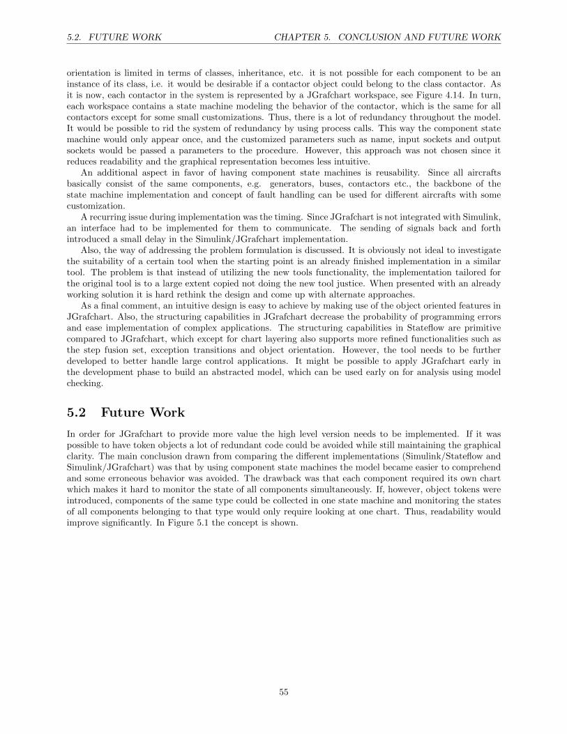
5.2. FUTURE WORK CHAPTER 5. CONCLUSION AND FUTURE WORK
orientation is limited in terms of classes, inheritance, etc. it is not possible for each component to be aninstance of its class, i.e. it would be desirable if a contactor object could belong to the class contactor. Asit is now, each contactor in the system is represented by a JGrafchart workspace, see Figure 4.14. In turn,each workspace contains a state machine modeling the behavior of the contactor, which is the same for allcontactors except for some small customizations. Thus, there is a lot of redundancy throughout the model.It would be possible to rid the system of redundancy by using process calls. This way the component statemachine would only appear once, and the customized parameters such as name, input sockets and outputsockets would be passed a parameters to the procedure. However, this approach was not chosen since itreduces readability and the graphical representation becomes less intuitive.
An additional aspect in favor of having component state machines is reusability. Since all aircraftsbasically consist of the same components, e.g. generators, buses, contactors etc., the backbone of thestate machine implementation and concept of fault handling can be used for different aircrafts with somecustomization.
A recurring issue during implementation was the timing. Since JGrafchart is not integrated with Simulink,an interface had to be implemented for them to communicate. The sending of signals back and forthintroduced a small delay in the Simulink/JGrafchart implementation.
Also, the way of addressing the problem formulation is discussed. It is obviously not ideal to investigatethe suitability of a certain tool when the starting point is an already finished implementation in a similartool. The problem is that instead of utilizing the new tools functionality, the implementation tailored forthe original tool is to a large extent copied not doing the new tool justice. When presented with an alreadyworking solution it is hard rethink the design and come up with alternate approaches.
As a final comment, an intuitive design is easy to achieve by making use of the object oriented features inJGrafchart. Also, the structuring capabilities in JGrafchart decrease the probability of programming errorsand ease implementation of complex applications. The structuring capabilities in Stateflow are primitivecompared to JGrafchart, which except for chart layering also supports more refined functionalities such asthe step fusion set, exception transitions and object orientation. However, the tool needs to be furtherdeveloped to better handle large control applications. It might be possible to apply JGrafchart early inthe development phase to build an abstracted model, which can be used early on for analysis using modelchecking.
5.2 Future Work
In order for JGrafchart to provide more value the high level version needs to be implemented. If it waspossible to have token objects a lot of redundant code could be avoided while still maintaining the graphicalclarity. The main conclusion drawn from comparing the different implementations (Simulink/Stateflow andSimulink/JGrafchart) was that by using component state machines the model became easier to comprehendand some erroneous behavior was avoided. The drawback was that each component required its own chartwhich makes it hard to monitor the state of all components simultaneously. If, however, object tokens wereintroduced, components of the same type could be collected in one state machine and monitoring the statesof all components belonging to that type would only require looking at one chart. Thus, readability wouldimprove significantly. In Figure 5.1 the concept is shown.
55
5.2. FUTURE WORK CHAPTER 5. CONCLUSION AND FUTURE WORK
Figure 5.1: Concept Of Object Tokens In JGrafchart
56

Part II
Modeling of IMA Control Systems
58

Chapter 6
Integrated Modular Avionics
6.1 Background and Introduction to IMA
Integrated Modular Avionics (IMA) is a term used for distributed computer networks in aircrafts and aconcept describing how to integrate distributed modules. In the aircraft industry today there is an increasingdrive towards IMA. One reason for this is that it replaces the point-to-point networking with virtual links andthus reduces the required wiring. This is an important improvement since the wires together with isolationare the main contributor to aircraft weight. Furthermore the weight of the aircraft is a key point of cost.Another important reason for using IMA is that it increases system reliance since the network protocol usedis deterministic and redundant.
In distributed computer networks it is not unusual for actuators, sensors and controllers to be on differentnetworks with different protocols. As control system complexity increases the ability of evaluation at an earlydesign stage is highly desirable. By being aware of the constraints both on control algorithm and software,developers can early on comment on system restrictions. From a cost perspective it is valuable to beable to analyze a system before it is a finished product, since adjustments grow more expensive with eachdevelopment phase.
In order to understand the effect of delay and jitter that might occur due to distribution, simulationtools are needed. Simulation tools can be used to investigate the constraints and possibilities of the system,with respect to the control algorithm as well as the software design. Delay and jitter might lead to poorcontrol performance, and therefore it is important to have an idea about how much interference the systemcan handle before becoming unstable.
As for the first part of the thesis, this part also aims to investigate the suitability of a certain tool on HSsystems, namely TrueTime. TrueTime is a Simulink-based simulation tool for real-time control applications.The main objectives of this part are to apply TrueTime to HS systems and to extend the TrueTime libraryto typical aircraft control systems that employ IMA. The motivation for doing this is that TrueTime thencould be used to build an abstracted model containing all critical elements, run simulations and analyze theimpact of delay and interference traffic on control performance. Furthermore, the analysis result can be usedto help drive requirements which normally are difficult to assess, already at a design stage [18].
6.2 Theory
6.2.1 Network Protocols
As mentioned, control systems are often distributed over different networks with different network protocols.This section aims to give a background on the protocols present in the system that was modeled in TrueTime.
TDMA
The Time Division Multiple Access (TDMA) is a communication channel access method which makes itpossible for several nodes to exchange data over the same frequency channel. The nodes on the network send
60
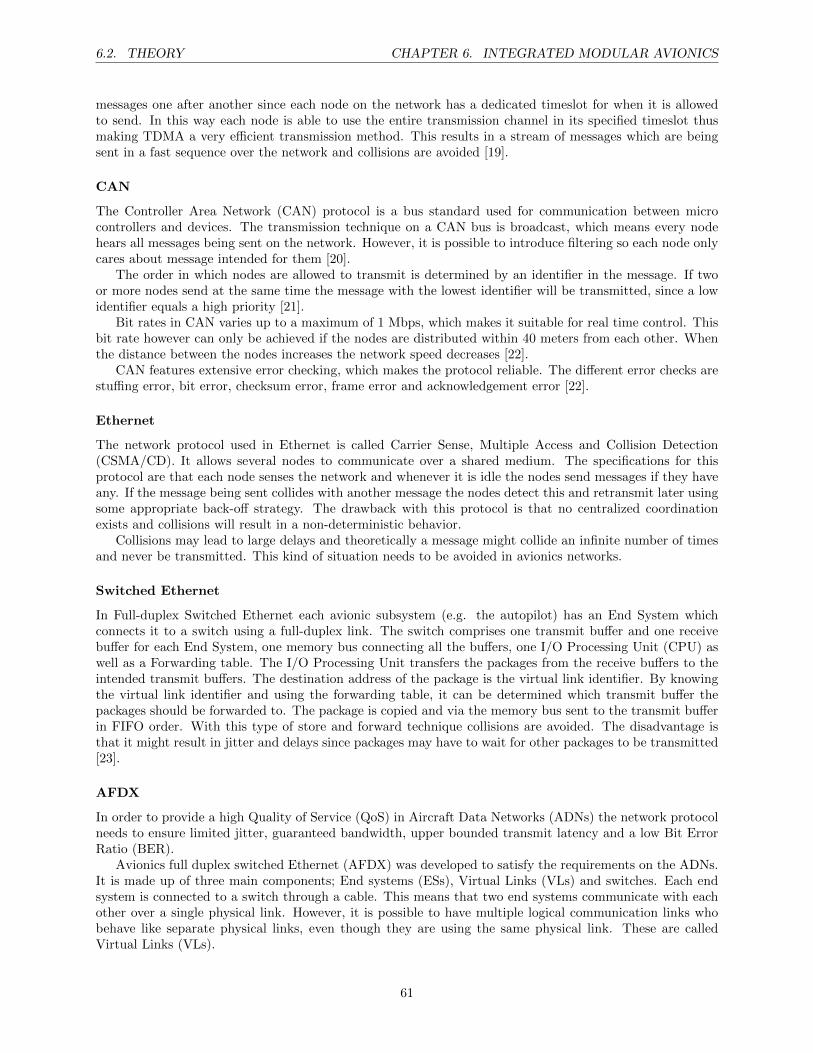
6.2. THEORY CHAPTER 6. INTEGRATED MODULAR AVIONICS
messages one after another since each node on the network has a dedicated timeslot for when it is allowedto send. In this way each node is able to use the entire transmission channel in its specified timeslot thusmaking TDMA a very efficient transmission method. This results in a stream of messages which are beingsent in a fast sequence over the network and collisions are avoided [19].
CAN
The Controller Area Network (CAN) protocol is a bus standard used for communication between microcontrollers and devices. The transmission technique on a CAN bus is broadcast, which means every nodehears all messages being sent on the network. However, it is possible to introduce filtering so each node onlycares about message intended for them [20].
The order in which nodes are allowed to transmit is determined by an identifier in the message. If twoor more nodes send at the same time the message with the lowest identifier will be transmitted, since a lowidentifier equals a high priority [21].
Bit rates in CAN varies up to a maximum of 1 Mbps, which makes it suitable for real time control. Thisbit rate however can only be achieved if the nodes are distributed within 40 meters from each other. Whenthe distance between the nodes increases the network speed decreases [22].
CAN features extensive error checking, which makes the protocol reliable. The different error checks arestuffing error, bit error, checksum error, frame error and acknowledgement error [22].
Ethernet
The network protocol used in Ethernet is called Carrier Sense, Multiple Access and Collision Detection(CSMA/CD). It allows several nodes to communicate over a shared medium. The specifications for thisprotocol are that each node senses the network and whenever it is idle the nodes send messages if they haveany. If the message being sent collides with another message the nodes detect this and retransmit later usingsome appropriate back-off strategy. The drawback with this protocol is that no centralized coordinationexists and collisions will result in a non-deterministic behavior.
Collisions may lead to large delays and theoretically a message might collide an infinite number of timesand never be transmitted. This kind of situation needs to be avoided in avionics networks.
Switched Ethernet
In Full-duplex Switched Ethernet each avionic subsystem (e.g. the autopilot) has an End System whichconnects it to a switch using a full-duplex link. The switch comprises one transmit buffer and one receivebuffer for each End System, one memory bus connecting all the buffers, one I/O Processing Unit (CPU) aswell as a Forwarding table. The I/O Processing Unit transfers the packages from the receive buffers to theintended transmit buffers. The destination address of the package is the virtual link identifier. By knowingthe virtual link identifier and using the forwarding table, it can be determined which transmit buffer thepackages should be forwarded to. The package is copied and via the memory bus sent to the transmit bufferin FIFO order. With this type of store and forward technique collisions are avoided. The disadvantage isthat it might result in jitter and delays since packages may have to wait for other packages to be transmitted[23].
AFDX
In order to provide a high Quality of Service (QoS) in Aircraft Data Networks (ADNs) the network protocolneeds to ensure limited jitter, guaranteed bandwidth, upper bounded transmit latency and a low Bit ErrorRatio (BER).
Avionics full duplex switched Ethernet (AFDX) was developed to satisfy the requirements on the ADNs.It is made up of three main components; End systems (ESs), Virtual Links (VLs) and switches. Each endsystem is connected to a switch through a cable. This means that two end systems communicate with eachother over a single physical link. However, it is possible to have multiple logical communication links whobehave like separate physical links, even though they are using the same physical link. These are calledVirtual Links (VLs).
61
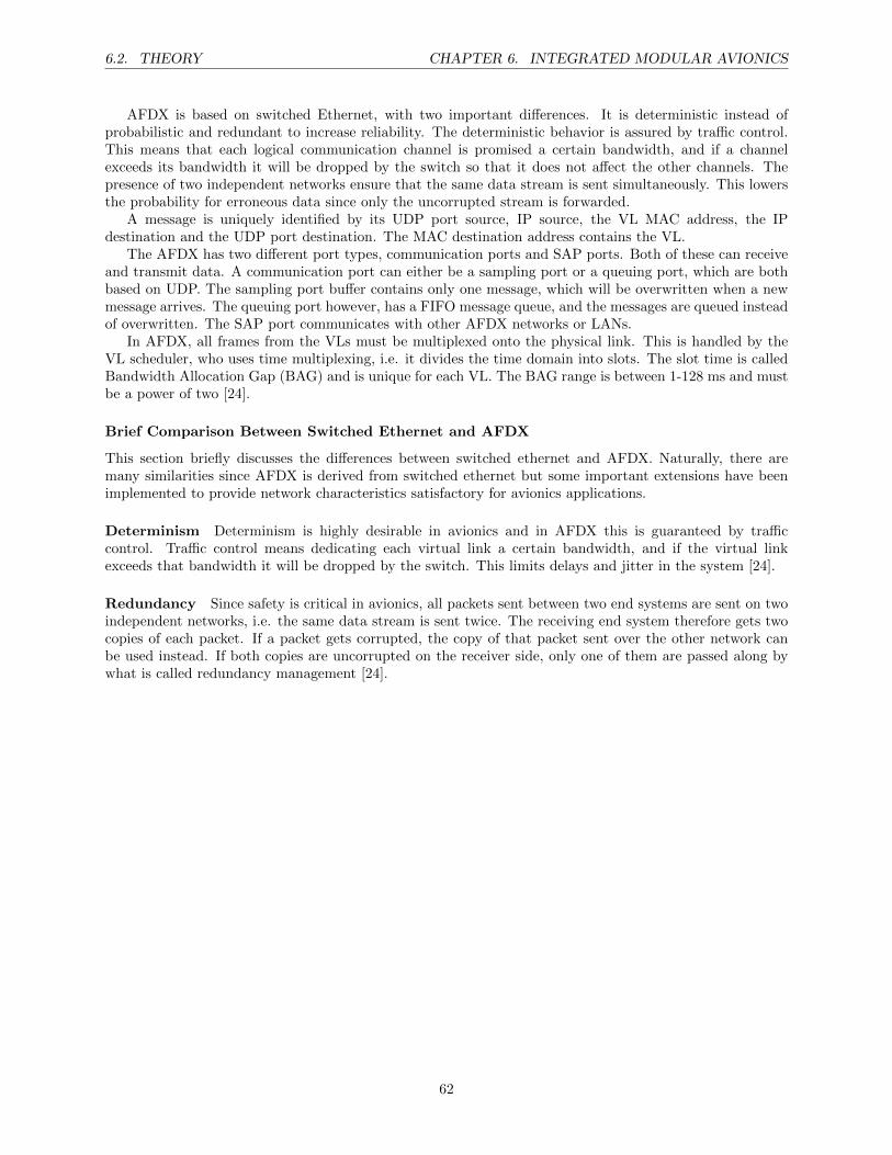
6.2. THEORY CHAPTER 6. INTEGRATED MODULAR AVIONICS
AFDX is based on switched Ethernet, with two important differences. It is deterministic instead ofprobabilistic and redundant to increase reliability. The deterministic behavior is assured by traffic control.This means that each logical communication channel is promised a certain bandwidth, and if a channelexceeds its bandwidth it will be dropped by the switch so that it does not affect the other channels. Thepresence of two independent networks ensure that the same data stream is sent simultaneously. This lowersthe probability for erroneous data since only the uncorrupted stream is forwarded.
A message is uniquely identified by its UDP port source, IP source, the VL MAC address, the IPdestination and the UDP port destination. The MAC destination address contains the VL.
The AFDX has two different port types, communication ports and SAP ports. Both of these can receiveand transmit data. A communication port can either be a sampling port or a queuing port, which are bothbased on UDP. The sampling port buffer contains only one message, which will be overwritten when a newmessage arrives. The queuing port however, has a FIFO message queue, and the messages are queued insteadof overwritten. The SAP port communicates with other AFDX networks or LANs.
In AFDX, all frames from the VLs must be multiplexed onto the physical link. This is handled by theVL scheduler, who uses time multiplexing, i.e. it divides the time domain into slots. The slot time is calledBandwidth Allocation Gap (BAG) and is unique for each VL. The BAG range is between 1-128 ms and mustbe a power of two [24].
Brief Comparison Between Switched Ethernet and AFDX
This section briefly discusses the differences between switched ethernet and AFDX. Naturally, there aremany similarities since AFDX is derived from switched ethernet but some important extensions have beenimplemented to provide network characteristics satisfactory for avionics applications.
Determinism Determinism is highly desirable in avionics and in AFDX this is guaranteed by trafficcontrol. Traffic control means dedicating each virtual link a certain bandwidth, and if the virtual linkexceeds that bandwidth it will be dropped by the switch. This limits delays and jitter in the system [24].
Redundancy Since safety is critical in avionics, all packets sent between two end systems are sent on twoindependent networks, i.e. the same data stream is sent twice. The receiving end system therefore gets twocopies of each packet. If a packet gets corrupted, the copy of that packet sent over the other network canbe used instead. If both copies are uncorrupted on the receiver side, only one of them are passed along bywhat is called redundancy management [24].
62

Chapter 7
TrueTime
7.0.2 TrueTime
Today it is common for systems to be distributed over multi-tasking kernel nodes, which communicate ondifferent networks. In these systems the nodes compete for the shared resources (The CPU and bandwidth)and the distribution of bandwidth is determined by the network protocol. Since the shared resources arelimited in terms of bandwidth different kinds of delays arise, such as transmission delays and back-off times.The delays might lower the control performance significantly, which is why it is important to identify themearly in the development process, preferably at the design stage. The bottom line is that both the controlalgorithm and control software need to be studied and taken into account simultaneously early on in thedevelopment process.
TrueTime is a simulation tool used for real-time systems and has been developed at Lund Universitysince 1999. Its main purpose is to analyze the impact of latency on control performance in networked controlapplications. TrueTime is based on Matlab/Simulink and applications can be built both as .cpp and .mfiles[18].
The TrueTime library comprises of several blocks which are briefly described below, as well as shown inFigure 7.1.
TrueTime Kernel In the kernel node, the user can define tasks which are either periodic or sporadic.For the sporadic tasks, there also need to be an interrupt handler defined since they are event-based. Thescheduling policy of the kernel is set by the user [18].
TrueTime Network The network blocks enable nodes to interchange data with each other using a specificnetwork protocol. The supported protocols for wired communication are Ethernet, CAN, TDMA, FDMA,Round Robin, Switched Ethernet, FlexRay and PROFINET [18].
TrueTime Wireless Network TrueTime also features a block for wireless communication. The protocolssupported are 802.11b WLAN and 802.15.4 ZigBee [18].
64
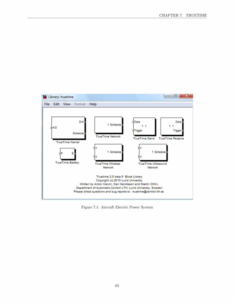
CHAPTER 7. TRUETIME
Figure 7.1: Aircraft Electric Power System
65
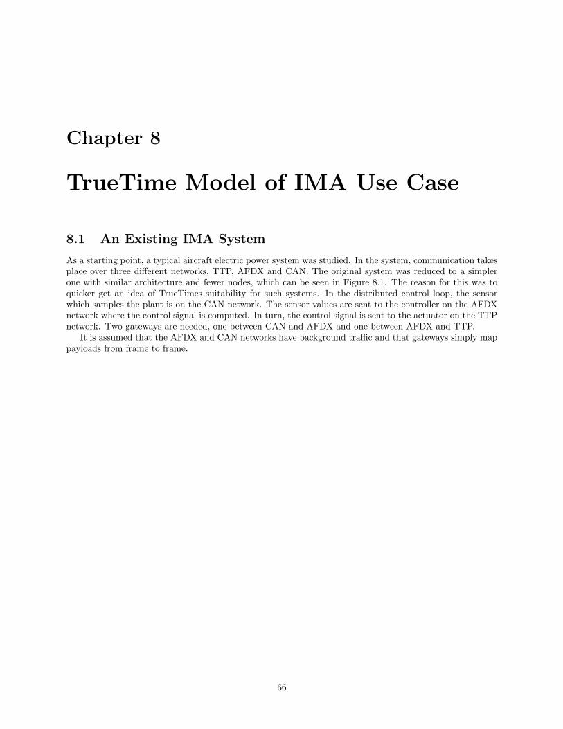
Chapter 8
TrueTime Model of IMA Use Case
8.1 An Existing IMA System
As a starting point, a typical aircraft electric power system was studied. In the system, communication takesplace over three different networks, TTP, AFDX and CAN. The original system was reduced to a simplerone with similar architecture and fewer nodes, which can be seen in Figure 8.1. The reason for this was toquicker get an idea of TrueTimes suitability for such systems. In the distributed control loop, the sensorwhich samples the plant is on the CAN network. The sensor values are sent to the controller on the AFDXnetwork where the control signal is computed. In turn, the control signal is sent to the actuator on the TTPnetwork. Two gateways are needed, one between CAN and AFDX and one between AFDX and TTP.
It is assumed that the AFDX and CAN networks have background traffic and that gateways simply mappayloads from frame to frame.
66
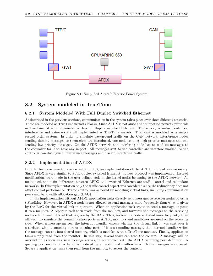
8.2. SYSTEM MODELED IN TRUETIME CHAPTER 8. TRUETIME MODEL OF IMA USE CASE
Figure 8.1: Simplified Aircraft Electric Power System
8.2 System modeled in TrueTime
8.2.1 System Modeled With Full Duplex Switched Ethernet
As described in the previous sections, communication in the system takes place over three different networks.These are modeled as TrueTime network blocks. Since AFDX is not among the supported network protocolsin TrueTime, it is approximated with a full duplex switched Ethernet. The sensor, actuator, controller,interference and gateways are all implemented as TrueTime kernels. The plant is modeled as a simplesecond order system. In order to simulate background traffic on the CAN network, interference nodessending dummy messages to themselves are introduced, one node sending high-priority messages and onesending low priority messages. On the AFDX network, the interfering node has to send its messages tothe controller for it to have any impact. All messages sent to the controller are therefore marked, so thecontroller can distinguish interference messages and discard interfering traffic.
8.2.2 Implementation of AFDX
In order for TrueTime to provide value for HS, an implementation of the AFDX protocol was necessary.Since AFDX is very similar to a full duplex switched Ethernet, no new protocol was implemented. Insteadmodifications were made in the user defined code in the kernel nodes belonging to the AFDX network. Asmentioned, the main differences between AFDX and switched Ethernet are traffic control and redundantnetworks. In this implementation only the traffic control aspect was considered since the redundancy does notaffect control performance. Traffic control was achieved by modeling virtual links, including communicationports and bandwidth allocation gap (BAG).
In the implementation without AFDX, application tasks directly send messages to receiver nodes by usingttSendMsg. However, in AFDX a node is not allowed to send messages more frequently than what is givenby the BAG for the virtual link in question. When an application task wants to send a message, it postsit to a mailbox. A separate task then reads from the mailbox, and forwards the messages to the receivingnodes with a time interval that is given by the BAG. Thus, no sending node will send more frequently thanallowed. To simulate the communication ports in AFDX, monitors and mailboxes are used on the receivingside. When a message arrives, the interrupt handler checks whether the virtual link it was sent over isassociated with a sampling port or queuing port. If it is a sampling message, the interrupt handler writesthe message content into shared memory, which is modeled with a TrueTime monitor. Finally, applicationtasks simply read from the monitor. In this way, several tasks can read the content. A message will beoverwritten as soon as a new message arrives, in accordance with the AFDX sampling port definition. Aqueuing port on the other hand, is modeled by an additional mailbox in which the messages are queued.Separate application tasks then read from the mailbox to access the content.
67
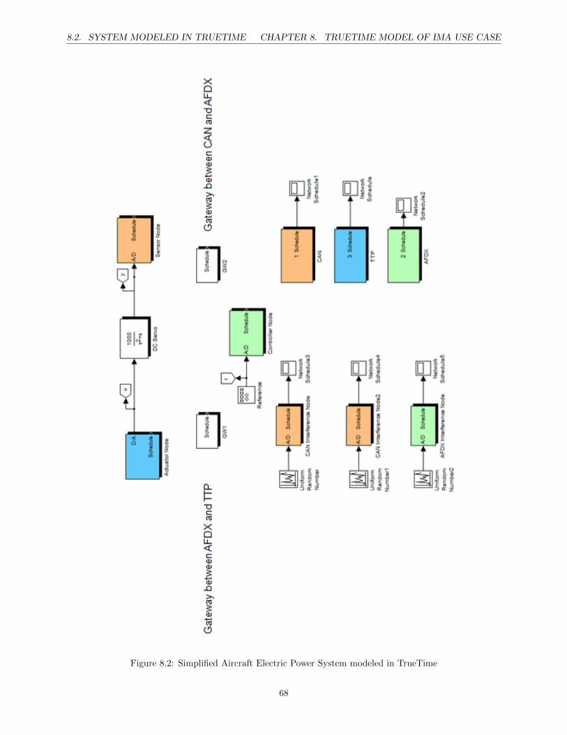
8.2. SYSTEM MODELED IN TRUETIME CHAPTER 8. TRUETIME MODEL OF IMA USE CASE
Figure 8.2: Simplified Aircraft Electric Power System modeled in TrueTime
68
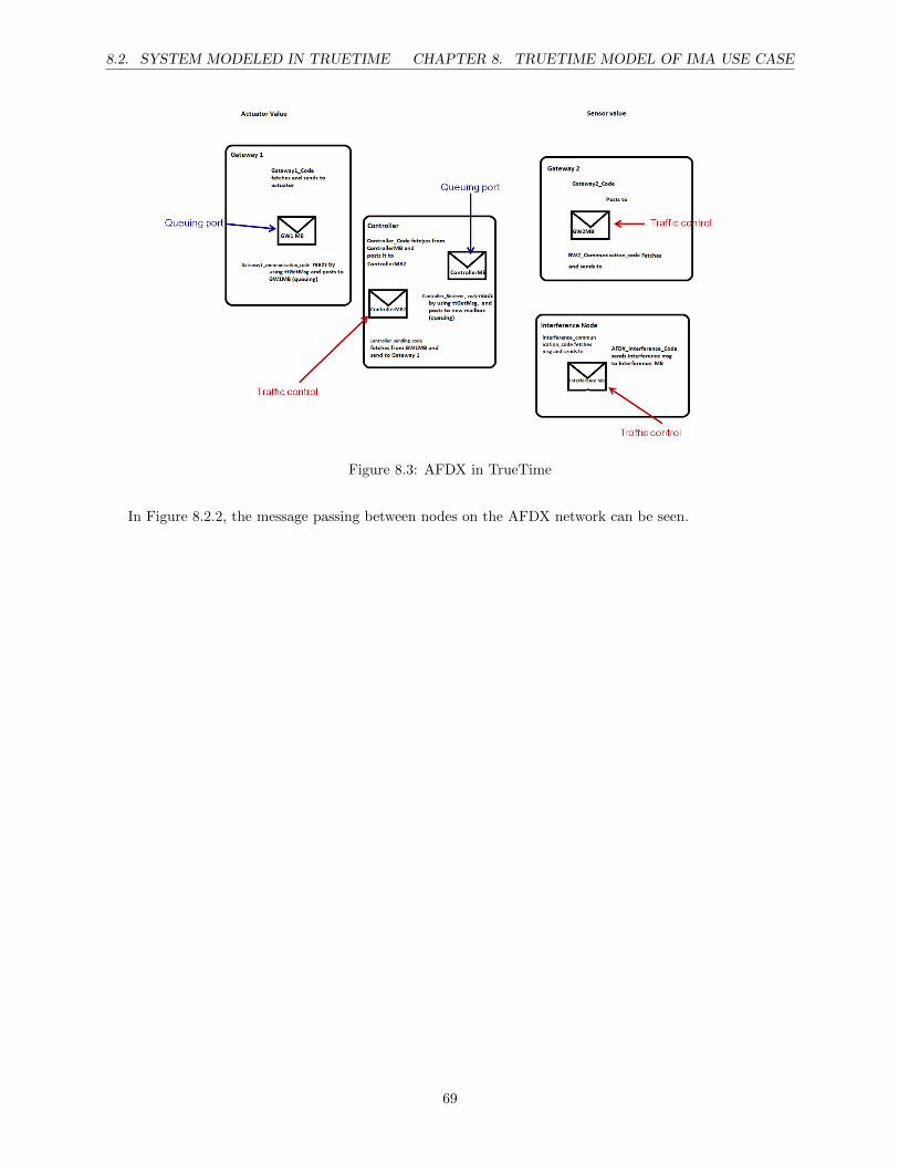
8.2. SYSTEM MODELED IN TRUETIME CHAPTER 8. TRUETIME MODEL OF IMA USE CASE
Figure 8.3: AFDX in TrueTime
In Figure 8.2.2, the message passing between nodes on the AFDX network can be seen.
69
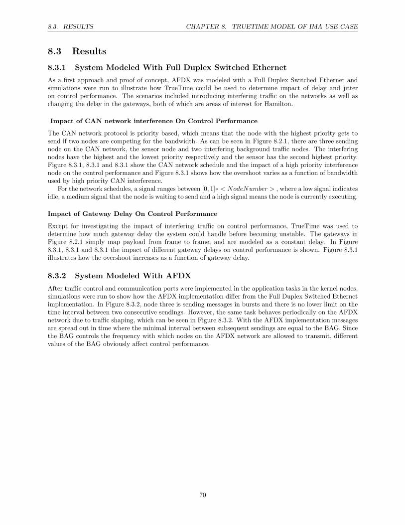
8.3. RESULTS CHAPTER 8. TRUETIME MODEL OF IMA USE CASE
8.3 Results
8.3.1 System Modeled With Full Duplex Switched Ethernet
As a first approach and proof of concept, AFDX was modeled with a Full Duplex Switched Ethernet andsimulations were run to illustrate how TrueTime could be used to determine impact of delay and jitteron control performance. The scenarios included introducing interfering traffic on the networks as well aschanging the delay in the gateways, both of which are areas of interest for Hamilton.
Impact of CAN network interference On Control Performance
The CAN network protocol is priority based, which means that the node with the highest priority gets tosend if two nodes are competing for the bandwidth. As can be seen in Figure 8.2.1, there are three sendingnode on the CAN network, the sensor node and two interfering background traffic nodes. The interferingnodes have the highest and the lowest priority respectively and the sensor has the second highest priority.Figure 8.3.1, 8.3.1 and 8.3.1 show the CAN network schedule and the impact of a high priority interferencenode on the control performance and Figure 8.3.1 shows how the overshoot varies as a function of bandwidthused by high priority CAN interference.
For the network schedules, a signal ranges between [0, 1]∗ < NodeNumber > , where a low signal indicatesidle, a medium signal that the node is waiting to send and a high signal means the node is currently executing.
Impact of Gateway Delay On Control Performance
Except for investigating the impact of interfering traffic on control performance, TrueTime was used todetermine how much gateway delay the system could handle before becoming unstable. The gateways inFigure 8.2.1 simply map payload from frame to frame, and are modeled as a constant delay. In Figure8.3.1, 8.3.1 and 8.3.1 the impact of different gateway delays on control performance is shown. Figure 8.3.1illustrates how the overshoot increases as a function of gateway delay.
8.3.2 System Modeled With AFDX
After traffic control and communication ports were implemented in the application tasks in the kernel nodes,simulations were run to show how the AFDX implementation differ from the Full Duplex Switched Ethernetimplementation. In Figure 8.3.2, node three is sending messages in bursts and there is no lower limit on thetime interval between two consecutive sendings. However, the same task behaves periodically on the AFDXnetwork due to traffic shaping, which can be seen in Figure 8.3.2. With the AFDX implementation messagesare spread out in time where the minimal interval between subsequent sendings are equal to the BAG. Sincethe BAG controls the frequency with which nodes on the AFDX network are allowed to transmit, differentvalues of the BAG obviously affect control performance.
70
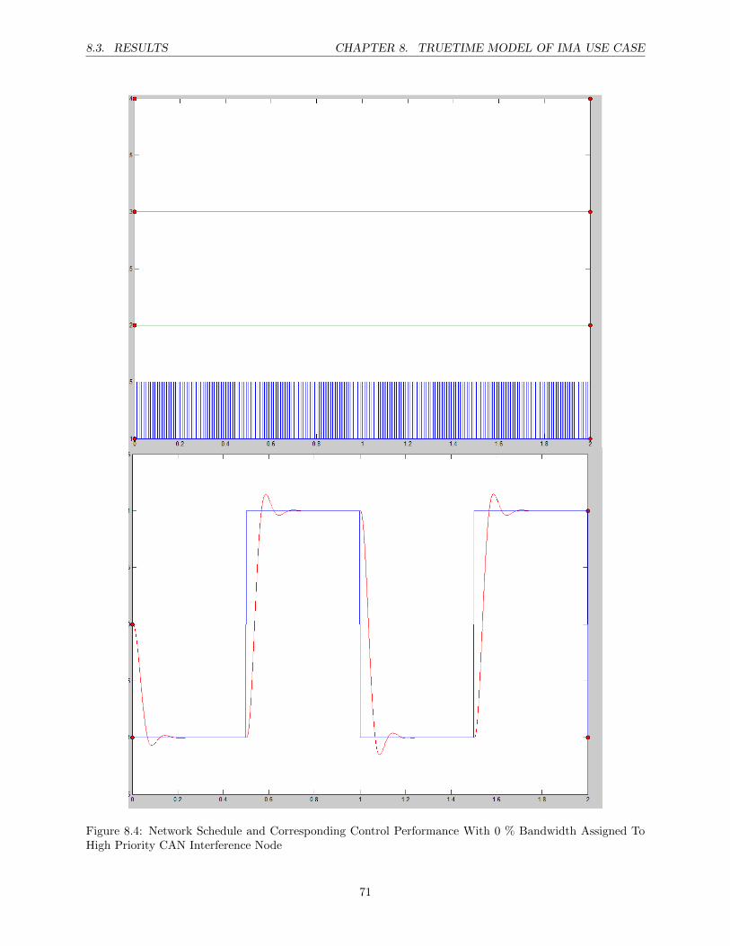
8.3. RESULTS CHAPTER 8. TRUETIME MODEL OF IMA USE CASE
Figure 8.4: Network Schedule and Corresponding Control Performance With 0 % Bandwidth Assigned ToHigh Priority CAN Interference Node
71
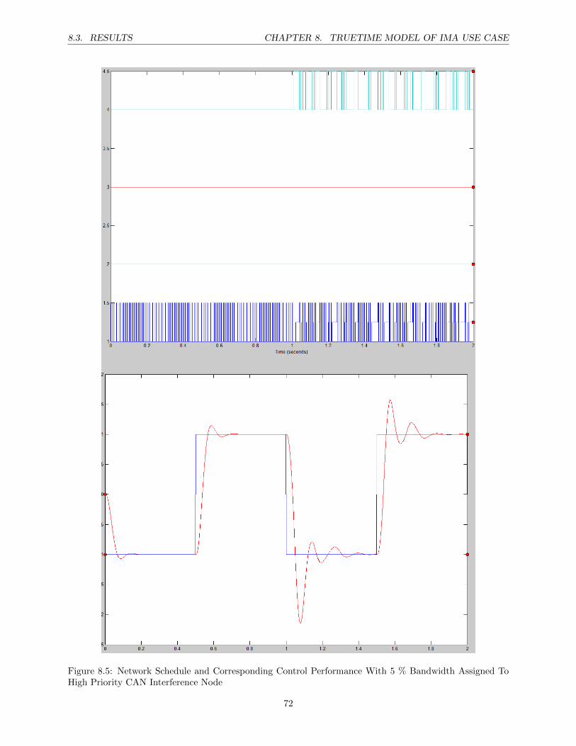
8.3. RESULTS CHAPTER 8. TRUETIME MODEL OF IMA USE CASE
Figure 8.5: Network Schedule and Corresponding Control Performance With 5 % Bandwidth Assigned ToHigh Priority CAN Interference Node
72
8.3. RESULTS CHAPTER 8. TRUETIME MODEL OF IMA USE CASE
Figure 8.6: Network Schedule and Corresponding Control Performance With 10 % Bandwidth Assigned ToHigh Priority CAN Interference Node
73
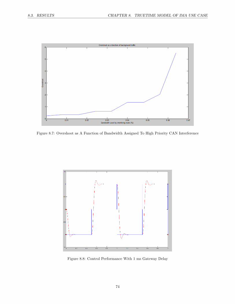
8.3. RESULTS CHAPTER 8. TRUETIME MODEL OF IMA USE CASE
Figure 8.7: Overshoot as A Function of Bandwidth Assigned To High Priority CAN Interference
Figure 8.8: Control Performance With 1 ms Gateway Delay
74
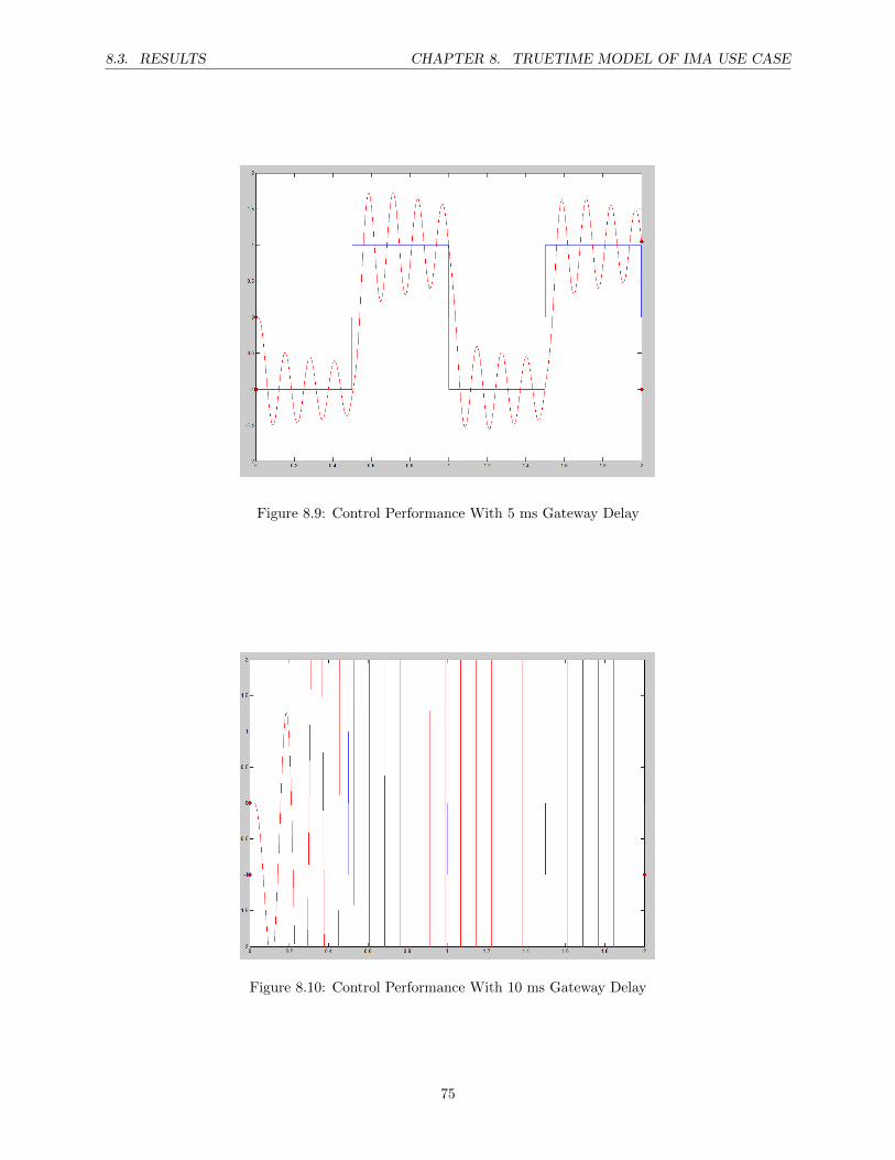
8.3. RESULTS CHAPTER 8. TRUETIME MODEL OF IMA USE CASE
Figure 8.9: Control Performance With 5 ms Gateway Delay
Figure 8.10: Control Performance With 10 ms Gateway Delay
75
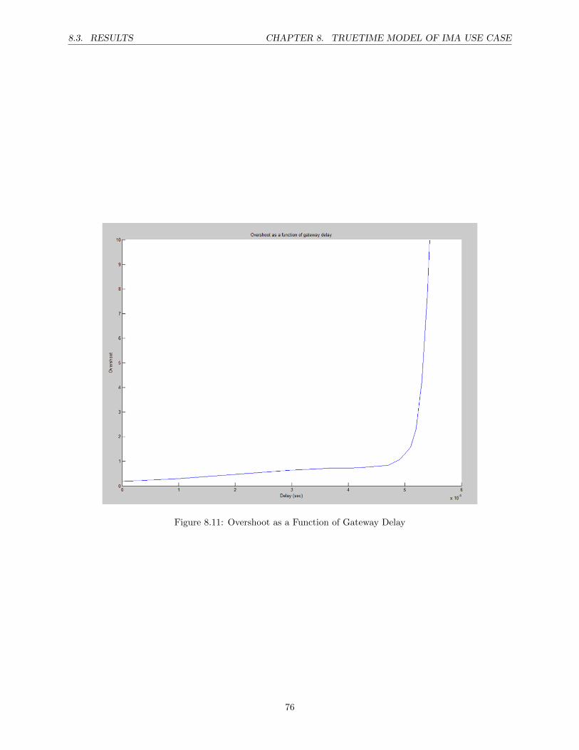
8.3. RESULTS CHAPTER 8. TRUETIME MODEL OF IMA USE CASE
Figure 8.11: Overshoot as a Function of Gateway Delay
76
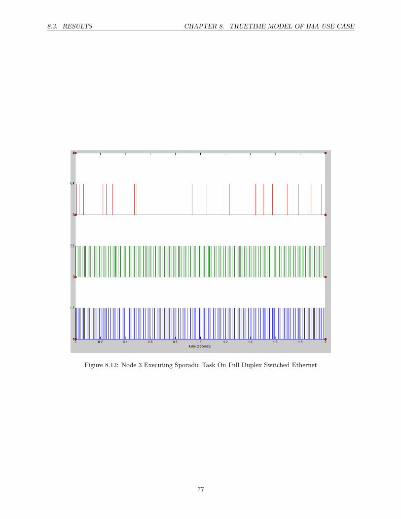
8.3. RESULTS CHAPTER 8. TRUETIME MODEL OF IMA USE CASE
Figure 8.12: Node 3 Executing Sporadic Task On Full Duplex Switched Ethernet
77
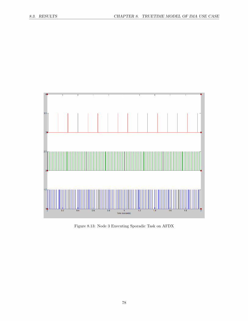
8.3. RESULTS CHAPTER 8. TRUETIME MODEL OF IMA USE CASE
Figure 8.13: Node 3 Executing Sporadic Task on AFDX
78
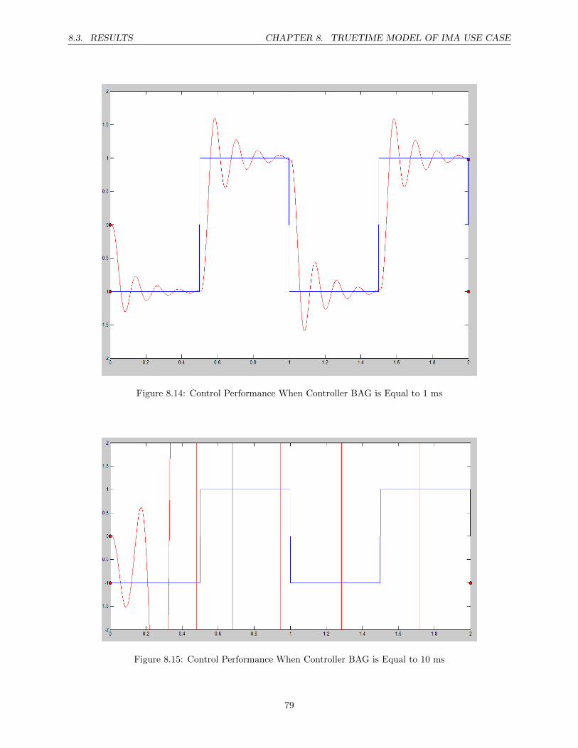
8.3. RESULTS CHAPTER 8. TRUETIME MODEL OF IMA USE CASE
Figure 8.14: Control Performance When Controller BAG is Equal to 1 ms
Figure 8.15: Control Performance When Controller BAG is Equal to 10 ms
79
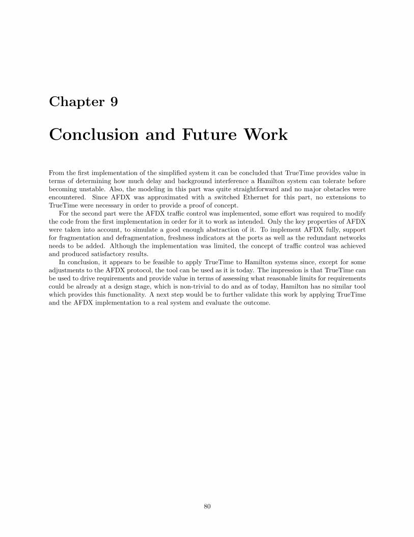
Chapter 9
Conclusion and Future Work
From the first implementation of the simplified system it can be concluded that TrueTime provides value interms of determining how much delay and background interference a Hamilton system can tolerate beforebecoming unstable. Also, the modeling in this part was quite straightforward and no major obstacles wereencountered. Since AFDX was approximated with a switched Ethernet for this part, no extensions toTrueTime were necessary in order to provide a proof of concept.
For the second part were the AFDX traffic control was implemented, some effort was required to modifythe code from the first implementation in order for it to work as intended. Only the key properties of AFDXwere taken into account, to simulate a good enough abstraction of it. To implement AFDX fully, supportfor fragmentation and defragmentation, freshness indicators at the ports as well as the redundant networksneeds to be added. Although the implementation was limited, the concept of traffic control was achievedand produced satisfactory results.
In conclusion, it appears to be feasible to apply TrueTime to Hamilton systems since, except for someadjustments to the AFDX protocol, the tool can be used as it is today. The impression is that TrueTime canbe used to drive requirements and provide value in terms of assessing what reasonable limits for requirementscould be already at a design stage, which is non-trivial to do and as of today, Hamilton has no similar toolwhich provides this functionality. A next step would be to further validate this work by applying TrueTimeand the AFDX implementation to a real system and evaluate the outcome.
80

Bibliography
[1] More Open Electrical Technologies (MOET), Final Report, Dec. 2009
[2] Johann Bals, Gerhard Hofer, Andreas Pfeiffer, Christian Schallert, Object-Oriented Inverse Modellingof Multi-Domain Aircraft Equipment Systems and Assessment with Modelica, pp. 377-384, Proceedingsof the 3rd International Modelica Conference, Linkping, November 3-4, 2003,
[3] T. Wongpiromsarn, Ufuk Topcu, and R. Murray, Formal synthesis of embedded control software forvehicle management systems, AIAA Infotech Aerospace, 2011.
[4] “Hamilton Sundstrand History” [Online] Available at: http://www.hamiltonsundstrand.com/About+Us/Historical+Timeline[Accessed June 13 2012]
[5] Moir, I., Seabridge, A., “Aircraft Systems” Mechanical, electrical, and avionics subsystems integration,pp. 139-153, Second Edition, Professional Engineering Publishing, UK 2001
[6] Holzmann, G., “Design and Validation of Computer Protocols” pp. 162-164, February 2007
[7] Amato,C., Bonet, B., Zilberstein, S., “Finite-State Controllers Based on Mealy Machines for Central-ized and Decentralized POMDPs”, pp 1-2, July 2010
[8] The Mathworks “Stateflow and Stateflow Coder” For Complex Logic and State Diagram Modeling,Version 5, pp. 2-6
[9] Murata, T., “Petri Nets; Properties, analysis and applications” pp. -, April 1989.
[10] Graph Theory Glossary [Online] Available at: http://www.utm.edu/departments/math/graph/glossary.html#d[Accessed March 12 2012]
[11] Johnsson, C., “A graphical language for batch control”, pp 21-65, Ph.D dissertation, ISRNLUTFD2/TFRT–1051–SE, Department of Automatic Control, Lund University, Sweden, March 1999.
[12] Bobbio, A., “System modelling with Petri nets”, Istituto Elettrotecnico Nazionale Galileo Ferraris,Italy, 1991
[13] Niu, J., Zou, J., Ren, A., “OOPN:AN OBJECT-ORIENTED PETRI NETS AND ITS INTEGRATEDDEVELOPMENT ENVIRONMENT”, 2010
[14] Arzen, K-E., Johnsson, C., “Grafchart and Grafcet” A COMPARISON BETWEEN TWO GRAPHI-CAL LANGUAGES AIMED FOR SEQUENTIAL CONTROL APPLICATIONS,
[15] Arzen, K-E., “JGrafchart user manual” , ver. 1.5, 2004
[16] Olsson, R., “Batch Control and Diagnosis”, pp 50-51 , Ph.D dissertation, ISRN LUTFD2/TFRT–1073–SE, Department of Automatic Control, Lund University, Sweden, June 2005.
[17] Arzen, K-E., Johnsson, C., “Grafchart and its relation to Grafcet and Petri nets”, 1998
[18] Cervin, A., Henriksson, D., Lincoln, B., Eker, J., Arzen, K-E., “How Does Control Timing AffectPerformance?” Analysis and Simulation of Timing Using Jitterbug and TrueTime, pp. -, June 2003.
82
BIBLIOGRAPHY BIBLIOGRAPHY
[19] Dhotre, I.A., Bagad, V.S., “Data Communication and Networking” ,pp. 287 , First Edition, TechnicalPublications Pune, August 2005
[20] The CAN protocol [Online] http://www.kvaser.com/en/about-can/the-can-protocol.html [Accessed:May 9 2012]
[21] Controller Area Network (CAN) [Online] http://www.ece.cmu.edu/ ece649/lectures/11 can.pdf [Ac-cessed: May 9 2012]
[22] CAN - A Brief Tutorial [Online] http://www.computer-solutions.co.uk/info/Embedded tutorials/can tutorial.htm[Accessed: May 9 2012]
[23] General Electric FANUC, “AFDX/ARINC 664 Protocol” Tutorial
[24] Techsat, “AFDX/ARINC 664” A Tutorial, August 2008
83