Embed Size (px)
Citation preview

Automatic Generation of2-AntWars Players with Genetic
Programming
DIPLOMARBEIT
zur Erlangung des akademischen Grades
Diplom-Ingenieur
im Rahmen des Studiums
Computational Intelligence
eingereicht von
Johannes InführMatrikelnummer 0625654
an derFakultät für Informatik der Technischen Universität Wien
BetreuungUniv.-Prof. Dr. Günther R. Raidl
Wien, 19.07.2010(Unterschrift Verfasser) (Unterschrift Betreuer)
Technische Universität WienA-1040 Wien � Karlsplatz 13 � Tel. +43-1-58801-0 � www.tuwien.ac.at


Erklärung zur Verfassung der Arbeit
Inführ JohannesKaposigasse 60, 1220 Wien
Hiermit erkläre ich, dass ich diese Arbeit selbständig verfasst habe, dass ich die verwende-ten Quellen und Hilfsmittel vollständig angegeben habe und dass ich die Stellen der Arbeit– einschließlich Tabellen, Karten und Abbildungen –, die anderen Werken oder dem Internetim Wortlaut oder dem Sinn nach entnommen sind, auf jeden Fall unter Angabe der Quelle alsEntlehnung kenntlich gemacht habe.
Wien, 19.07.2010(Inführ Johannes)
Acknowledgements
In no particular order I would like to thank Univ.-Prof. Dr. Günther R. Raidl for allowing me todo research on a topic of my own choice and his continued support and encouragement duringthe creation of this thesis. The advice that stuck with me the most was that voodoo is never asatisfactory explanation of strange software errors. My girlfriend and my family have my eternalgratitude for letting me code day in and day out, encouraging me when the work seemed neverending and paying the electricity bill I racked up, and of course big thanks to everyone whorefrained from dousing me in insecticide whenever I was talking nonstop about swarming ants.
i

Abstract
In the course of this thesis, the feasibility of automatically creating players for the game2-AntWars is studied. 2-AntWars is a generalization of AntWars which was introduced aspart of a competition accompanying the Genetic and Evolutionary Computation Conference2007. 2-AntWars is a two player game in which each player has control of two ants on aplaying field. Food is randomly placed on the playing field and the task of the players is tocollect more food than the opponent.
To solve this problem a model of the behaviour of a 2-AntWars player is developedand players are built according to this model by means of genetic programming, which is apopulation based evolutionary algorithm for program induction. To show the feasibility ofthis approach, the players are evolved in an evolutionary setting against predefined strategiesand in a coevolutionary setting where both players of 2-AntWars evolve and try to beat eachother.
Another core part of this thesis is the analysis of the evolutionary and behavioural dy-namic emerging during the development of 2-AntWars players. This entails specific char-acteristics of those players (e.g. which ant found how much food) and on a higher level theirbehaviour during games and the adaption to the behaviour of the opponent.
The results showed that it is indeed possible to create successful 2-AntWars players thatare able to beat fixed playing strategies that oppose them. This is a solution to an importantproblem of game designers as a well balanced game needs to have a feasible counter strategyto every strategy and with the help of the proposed method such counter strategies can befound automatically.
The attempt to create 2-AntWars players from scratch by letting the developed playersbattle each other was also successful. This is a significant result as it shows how to auto-matically create artificial intelligence for games (and in principle for any problems that canbe formulated as games) from scratch.
The developed solutions to the 2-AntWars problem were surprisingly diverse. Antswere used as bait, were hidden or shamelessly exploited weaknesses of the opponent. Thepopulation model that was chosen enabled the simultaneous development of players withdifferent playing strategies inside the same population without resorting to any special mea-sures normally associated with that like explicitly protecting a player using one strategyfrom a player using another one. Both mutation and crossover operators were shown to beessential for the creation of high performing 2-AntWars players.
ii
Zusammenfassung
Im Rahmen dieser Arbeit wird die Möglichkeit der automatischen Generierung vonSpielern für das Spiel 2-AntWars untersucht. 2-AntWars ist eine Generalisierung von Ant-Wars. AntWars wurde für einen Wettbewerb der Genetic and Evolutionary ComputationConverence 2007 erfunden. 2-AntWars ist ein Spiel für zwei Spieler, wobei jeder Spielerdie Kontrolle über zwei Ameisen auf einem Spielfeld hat. Auf diesem Spielfeld ist Futteran zufälligen Orten platziert und die Aufgabe der Spieler ist es, mehr Futter zu finden alsder jeweilige Gegner.
Um das Problem zu lösen wird ein Modell für das Verhalten eines 2-AntWars Spie-lers entwickelt und Genetic Programming, eine populationsbasierte evolutionäre Methodezur Programminduktion, wird verwendet um Spieler basierend auf diesem Modell zu er-stellen. Die Machbarkeit dieses Ansatzes wird gezeigt, indem Spieler sowohl per Evolutionim Kampf gegen fixe Spielstrategien als auch per Koevolution im Kampf gegeneinanderentwickelt werden.
Ein weiterer Kernpunkt dieser Arbeit ist die Analyse der Dynamik die während derEntwicklung der Spieler auftritt, sowohl von der evolutionären Perspektive als auch vonden zur Schau gestellten Verhaltensweisen der Spieler her. Das beinhaltet spezielle Eigen-schaften der Spieler (wie zum Beispiel welche Ameise wieviel Futter sammelt) aber auchdie Strategien der Spieler auf höherer Ebene und wie sie sich an ihre Gegner anpassen.
Die Ergebnisse zeigen, dass es in der Tat möglich ist erfolgreiche 2-AntWars Spielerzu erzeugen die in der Lage sind, fixe Strategien ihrer Gegner zu schlagen. Das ist ein Re-sultat das vor allem für Spieldesign-Probleme wichtig ist, da es für eine gute Spiel-Balanceunumgänglich ist, dass für jede Spielstrategie eine Gegenstrategie existiert. Mit Hilfe derdargelegten Methode ist es möglich, solche Gegenstrategien automatisiert aufzufinden.
Der Versuch 2-AntWars Spieler von Grund auf durch Spiele gegeneinander zu entwi-ckeln war ebenfalls von Erfolg gekrönt. Das zeigt, dass es möglich ist, künstliche Intelligenzfür Spiele (und im Prinzip für alle Probleme die als Spiele formuliert werden können) zuerzeugen, ohne Spielstrategien von Hand entwerfen zu müssen.
Die Verhaltensweisen die die entwickelten 2-AntWars Spieler an den Tag legten warenüberraschend vielfältig. Ameisen wurden als Köder verwendet, versteckt und wurden ge-nerell verwendet um Schwächen im Spiel des Gegners schamlos auszunutzen. Das gewähl-te Populationsmodell machte die simultane Entwicklung von Spielern mit verschiedenenSpielstrategien in derselben Population möglich, ohne dies explizit zu fördern, beispiels-weise indem Spieler einer Strategie vor Spielern einer anderen Strategie geschützt werden.Es zeigte sich, dass sowohl Mutations- als auch Crossover-Operationen für die Entwicklungvon leistungsfähigen 2-AntWars Spielern notwendig sind.
iii

Contents
Abstract ii
Zusammenfassung iii
Contents v
I Introduction 1
1 Introduction 3
2 Genetic Programming and Coevolution 5
3 2-AntWars 113.1 AntWars Rules . . . . . . . . . . . . . . . . . . . . . . . . . . . . . . . . . . 113.2 2-AntWars Rules . . . . . . . . . . . . . . . . . . . . . . . . . . . . . . . . . 123.3 Strategies . . . . . . . . . . . . . . . . . . . . . . . . . . . . . . . . . . . . . 14
II Genetic Programming System 17
4 Genetic Programming System 194.1 The GP-Algorithm . . . . . . . . . . . . . . . . . . . . . . . . . . . . . . . . 194.2 Individual Structure . . . . . . . . . . . . . . . . . . . . . . . . . . . . . . . . 194.3 Population Model . . . . . . . . . . . . . . . . . . . . . . . . . . . . . . . . . 214.4 Population Initialization . . . . . . . . . . . . . . . . . . . . . . . . . . . . . . 224.5 Selection . . . . . . . . . . . . . . . . . . . . . . . . . . . . . . . . . . . . . 224.6 Crossover . . . . . . . . . . . . . . . . . . . . . . . . . . . . . . . . . . . . . 224.7 Mutation . . . . . . . . . . . . . . . . . . . . . . . . . . . . . . . . . . . . . . 234.8 Evaluation . . . . . . . . . . . . . . . . . . . . . . . . . . . . . . . . . . . . . 24
5 Modelling the 2-AntWars Player 255.1 Data Types . . . . . . . . . . . . . . . . . . . . . . . . . . . . . . . . . . . . 265.2 Available Statements . . . . . . . . . . . . . . . . . . . . . . . . . . . . . . . 285.3 Belief Function . . . . . . . . . . . . . . . . . . . . . . . . . . . . . . . . . . 33
v

5.4 Predict Functions . . . . . . . . . . . . . . . . . . . . . . . . . . . . . . . . . 335.5 Movement Functions . . . . . . . . . . . . . . . . . . . . . . . . . . . . . . . 345.6 Decision Function . . . . . . . . . . . . . . . . . . . . . . . . . . . . . . . . . 355.7 Settings . . . . . . . . . . . . . . . . . . . . . . . . . . . . . . . . . . . . . . 36
III Results 39
6 No Adversary 416.1 Fitness development . . . . . . . . . . . . . . . . . . . . . . . . . . . . . . . 416.2 Belief . . . . . . . . . . . . . . . . . . . . . . . . . . . . . . . . . . . . . . . 466.3 Prediction . . . . . . . . . . . . . . . . . . . . . . . . . . . . . . . . . . . . . 476.4 General Performance Observations . . . . . . . . . . . . . . . . . . . . . . . . 486.5 Best Individuals . . . . . . . . . . . . . . . . . . . . . . . . . . . . . . . . . . 516.6 Conclusion . . . . . . . . . . . . . . . . . . . . . . . . . . . . . . . . . . . . 52
7 Strategies Version 1 537.1 Greedy . . . . . . . . . . . . . . . . . . . . . . . . . . . . . . . . . . . . . . . 537.2 Scorched Earth . . . . . . . . . . . . . . . . . . . . . . . . . . . . . . . . . . 607.3 Hunter . . . . . . . . . . . . . . . . . . . . . . . . . . . . . . . . . . . . . . . 67
8 Strategies Version 2 738.1 Greedy . . . . . . . . . . . . . . . . . . . . . . . . . . . . . . . . . . . . . . . 738.2 Scorched Earth . . . . . . . . . . . . . . . . . . . . . . . . . . . . . . . . . . 798.3 Hunter . . . . . . . . . . . . . . . . . . . . . . . . . . . . . . . . . . . . . . . 84
9 Coevolutionary Runs 919.1 Run with Standard Settings . . . . . . . . . . . . . . . . . . . . . . . . . . . . 919.2 Run with Asymmetric Evaluation . . . . . . . . . . . . . . . . . . . . . . . . . 979.3 Long Run . . . . . . . . . . . . . . . . . . . . . . . . . . . . . . . . . . . . . 1019.4 Long Run with Asymmetric Evaluation . . . . . . . . . . . . . . . . . . . . . 104
10 Special Analysis 10510.1 Mixed Opponent Strategies . . . . . . . . . . . . . . . . . . . . . . . . . . . . 10510.2 Stability of Results . . . . . . . . . . . . . . . . . . . . . . . . . . . . . . . . 10710.3 Playing against Unknown Opponents . . . . . . . . . . . . . . . . . . . . . . . 109
11 Conclusion 115
IV Appendix 119
A Strategy Evaluation 121
Bibliography 125
vi

Part I
Introduction

CHAPTER 1Introduction
The main aim of this thesis is to generalize AntWars [1] to 2-AntWars and to show how toautomatically create artificial intelligence capable of playing this new game. 2-AntWars is atwo-player game. Each player controls two ants on a rectangular playing field and tries to collectmore randomly distributed food than the opponent. Chapter 3 on page 11 describes the rules of2-AntWars and how they were derived from AntWars in detail.
Being able to automatically generate competent artificial intelligence has a lot of advantages.Since this thesis uses it to play a game, the first group of advantages directly concerns gamedevelopment. The most obvious one is to use the developed artificial intelligence as opponent forhumans in single-player games and skip the complex task of handcrafting an artificial opponent.However, there are equally important uses for automated gameplay during the development ofa game. For instance, one of the first steps of creating a game is to define its rules. The rulesdetermine under which conditions certain actions are available to the player. The authors of [2]describe two pitfalls when defining the rules of a game. The first one is that the rules are chosenin a way that a dominant strategy, which is a sequence of actions that always leads to victory,exists. In this situation, the player of the game simply has to execute this strategy to win, no skillor adaption to the current game situation is required. Dominant strategies make a game boringand as a consequence unsuccessful. The second pitfall is the availability of actions that arenever advantageous. After the player learns of them he will of course avoid them, making theirdefinition and implementation a waste of time and effort. The only way to avoid those pitfalls(especially for games with complex rules) is to play the game and try to find dominant strategiesand useless actions. This is a costly and time intensive process if humans are involved. With amethod to automatically create players for a game, the search for dominant strategies and uselessactions can be sped up immensely. If a player cannot be beaten by any other player, a dominantstrategy has been discovered. If an action is never used by any of the players, a useless actionhas been uncovered. With an automated method to create players it becomes easier to try a lotof different rules and evaluate their effect on the set of successful strategies. Improved testingof the game implementation is an additional benefit. Salge et al. [2] describe the developmentof strategies that crashed the game because that meant that they did not lose it. Automatically
3

CHAPTER 1. INTRODUCTION
created strategies will try everything that might give them an advantage, without being as biasedas human players. As a result, game situations that were not anticipated by the game designerand subsequently are not handled correctly by the game logic may arise. This of course doesnot mean that testing by humans becomes unnecessary, there are whole classes of problems thatautomatic strategy generation cannot uncover. For example, the method presented in this thesisuses the set of actions that the game rules specify to build strategies. It does not know what theactions are supposed to do, it simply chooses actions that are beneficial. If an action that shouldbe beneficial is actually detrimental because of an implementation error, the developed strategieswill try to work around that and the error remains unnoticed.
Automatic generation of artificial intelligence is not only applicable in various stages ofgame development. It can also be used to solve real world problems, especially if they can beformulated as a game or an agent based description is available. Imagine two competing com-panies A and B. A wants to lure customers away from B. It has various actions at its disposals.It can improve the own product, start a marketing campaign and place advertisements in variousmedia and at different physical locations or denounce the products of B. B can react in a lot ofdifferent ways to this and A wants to be able to anticipate possible reactions. Based on previousattempts to improve the market share, A has an elaborate model of the behaviour of the potentialcustomers. The game is based on this model. A uses its planned strategy as one player andan automatically generated strategy as approximation of the behaviour of B. The company thatincreases its market share wins. The automatically created strategies for B give A an insightinto the weaknesses of its own strategy. The game can also be reversed, the current marketingstrategy of B is implemented as a fixed player and strategies of A are automatically developedso that A has a good answer to B’s marketing.
The method used in this thesis to automatically create gaming strategies is genetic program-ming, an evolutionary algorithm that applies the principles of biological evolution to computerprograms. Using genetic programming to develop players of a game is not a particularly newidea. Even the first book of John Koza [3] (the inventor of genetic programming) contained theautomatic generation of a movement strategy for an ant that that tries to follow a path of food(artificial ant) and a lot of research has been done since then. Already mentioned was the workpresented in [2] where genetic programming was used to develop players of a turn based strat-egy game. In [4] space combat strategies were created. Other forms of predator-prey interactionwere analyzed in [5] and [6]. Genetic programming has also been used to develop soccer [7] andchess end game players [8]. However, the conducted research is focused on the end result andemerging evolutionary dynamics that occur during the development are neglected. In this thesisnot only the end results of evolution, but also the developments that led to those results will bepresented to gain insight into the evolutionary process of genetic programming.
The next chapter will introduce the central concepts of genetic programming. Chapter 3contains the complete definition of 2-AntWars and a discussion of possible strategies for thisgame. This is followed by a description of the genetic programming implementation that wasused for this thesis in chapter 4 and the 2-AntWars player model in chapter 5. Chapters 6 to9 contain the main results of this thesis, which are supplemented by experiments reported inchapter 10. A summary and directions for future work can be found in chapter 11.
4

CHAPTER 2Genetic Programming and Coevolution
Genetic programming is an evolutionary algorithm (EA) variant developed by John Koza [3].The primary difference between genetic programming and other EAs is the representation of anindividual. While individuals of genetic algorithms or evolution strategies are typically fixed-length vectors of numbers, genetic programming individuals (in their original form) are programtrees of variable structure. The program trees consist of functions and terminals. The leaf nodesare terminals and all inner nodes are functions. The children of functions supply the argumentsof the function when a program tree gets evaluated. A simple example is shown in figure 2.1.
Figure 2.1: Example of an genetic programming solution. The arguments of the binary + func-tion are supplied by the terminals 4 and 3.
A genetic programming implementation is supplied with a set of functions and terminalsthat it can use to solve a problem. One important constraint for the functions and terminals isthe closure property: every argument of every function can be supplied by every function andterminal available without producing an error. One consequence of this is that, for example,even when the dividend that is supplied to a division function is zero the result has to be defined.
A program tree is not the only possibility of representing a program, over time other rep-resentations have been developed. In [9] a stack based program representation is introduced.An individual is a simple vector of operations. These operations are executed on a virtual stack-based machine. Every operator pops its arguments from the execution stack and pushes its result.If the stack does not contain enough arguments the operation is ignored. Flow control is hardto achieve with this type of representation. Linear genetic programming [10] uses a similar vec-
5

CHAPTER 2. GENETIC PROGRAMMING AND COEVOLUTION
tor representation, the critical difference is that the arguments of the operations are supplied bymemory cells, much like native assembler code. Before the individual is executed, the memorycells are initialized with input values. The individual manipulates the memory during executionand the output is read from one or more memory cells designated as output. This representationalso has problems with flow control. The work cited uses a special operation that conditionallyskips the next (and only the next) operation which eases the implementation of the crossoveroperator. Cartesian genetic programming [11] uses a radically different approach to map anindividual to a program because it uses a genotype to phenotype transformation. The genotype(the individual) is a list of indices which specify the connections between a fixed number of logicgates and global inputs and outputs. The indices define for each gate which operation it uses andwhich gates (or global inputs) supply the necessary arguments for the operation. The indicesalso determine which gates are connected to the global output. The connected gates constitutethe phenotype, i.e. the program. Other types of genetic programming include parallel distributedgenetic programming [12] and grammatically-based genetic programming [13].
A variant of genetic programming that will be important for this thesis is strongly typedgenetic programming [14]. It removes the closure constraint by assigning types to the argu-ments and return values of functions and terminals. During the construction of individuals, onlyfunctions or terminals with a compatible return type are used as arguments of a parent function.Applied to the individual of figure 2.1 on the preceding page this means that the children of the+-function have to return numbers (like the terminals 4 and 3). A terminal returning a color forinstance would not be considered.
Genetic programming was successfully applied to a lot of problems, but it is not withoutits flaws. First and foremost, [15] cites that in most cases the function and terminal set usedfor solving a problem is not turing equivalent, i.e. misses loops and memory. In the work thatincluded loop constructs, only at most two nested loops were evolved. The authors argue thatevolving loops is a hard problem because small errors inside the body of a loop accumulate tolarge errors after multiple iterations. Building implicit loops out of lower level constructs likeconditional jumps is even harder. Another focus of critique is the crossover operation as it lackscontext information to select a useful part of one program and insert it at a suitable location inanother program. In [16] the headless chicken crossover (no crossover at all but replacing a partof a program with randomly created code) outperforms the normal crossover operation.
Apart from these weaknesses, genetic programming typically has the problem of code bloat,i.e. programs grow in size without increasing their fitness which causes performance deteriora-tion. In [17] and [18] six different theories of code bloat are discussed that were proposed overthe years, but there is no single conclusive reason for code bloat. Those theories are:
hitchhiking: The hitchhiking theory states that code bloat occurs because introns (code seg-ments without influence on the fitness of the program) that are near to advantageous codesegments spread with them through the population of programs.
defence against crossover: According to the defense against crossover theory, code bloatemerges because large programs with a lot of intron code are more likely to survive thedestructive effects of a crossover than small programs.
removal bias: Code removals by crossover are only allowed to be as large as an inactive codesegment to not influence the fitness of the individual. However, intron code insertions by
6

crossover do not have any size restrictions, which causes code bloat. This argument issimilar to the defense against crossover theory.
fitness causes bloat: The fitness causes bloat theory sees fitness as the driving factor of codebloat as experiments with random selection (without any regard for fitness) showed acomplete absence of code bloat.
modification point depth: It was observed that the effect of a crossover on the fitness corre-lates with the depth of the crossover point, deeper crossover points have a smaller ef-fect. Therefore large programs have an advantage because they can have deeper crossoverpoints, which is the core argument of the modification point depth theory.
crossover bias: The crossover bias theory concentrates on the fact that repeated application ofthe standard subtree crossover operator creates a lot of small programs. Because smallprograms are generally unfit they are discarded and the average program size of the pop-ulation rises, causing bloat.
Fitting for the high number of bloat theories, there are a lot of methods that aim at controllingbloat. The goal is to increase the parsimony of the found solutions or to make the evaluationof programs faster and therefore generate better solutions in the same timeframe. The bloatcontrol originally used by Koza was a fixed limit on program tree depth. Of course, limitingthe size (in total number of nodes) of a program tree is also an option. Size limits can alsobe applied to the whole population instead of each individual. Those limits can be static ordynamic, i.e. adapting to the current needs. There is a large number of parsimony pressuremethods that produce selective pressure towards small programs. One of them is lexicographicparsimony pressure which prefers the smaller program when two programs with otherwise equalfitness are compared. Other methods punish large programs by delaying their introduction intothe population or rising their probability of being discarded. Editing the programs to removeintron code is also possible to combat code growth but this can lead to premature convergence.The genetic operators are usually fixed but to mitigate code growth they can also be chosendynamically, larger (depending on size or depth) functions are changed by operators that aremore destructive. In this work, a combination of static size limits (based on the node count) andlexicographic parsimony pressure is chosen.
The second important concept necessary for this work besides genetic programming is co-evolution. It refers to any situation in which the evaluation of multiple populations is dependenton each other. It is useful for competitive problems or problems for which an explicit fitnessfunction is not known or hard to define [19]. In the domain of competitive problems, coevolu-tion is motivated by evolutionary arms races. Two or more species constantly try to beat eachother, developing higher and higher levels of complexity and performance. Coevolution can alsobe used to solve cooperative problems [20] by training teams of individuals. Each team mem-ber only has to solve a sub-problem. The central aspect of coevolution is the evaluation. Sinceno fitness measure is available, how can be determined which individuals are superior to allowany kind of progress? The answer is that the individuals of another population take the role ofperformance measure and to judge the fitness of one individual, it is pitted against other individ-uals. The intuitive solution to evaluate every individual against every other individual (completeevaluation) is usually impractical because it requires a quadratic amount of evaluations (in termsof population size) so some alternatives were developed. One of those is “All vs Best”. Each in-
7

CHAPTER 2. GENETIC PROGRAMMING AND COEVOLUTION
dividual is evaluated by pitting it against the best individual of the previous generation. Anotherone is tournament evaluation [21]. The individuals of the population are paired up and evaluated.The better individual advances to the next round and is paired up with another individual thatadvanced from the first round. The fitness of each individual is determined by how long it stayedin the tournament.
Even though coevolution is an elegant evolutionary approach in theory, it often exhibits somerather unpleasant pathologies in practice [22, 23]:
cycling: especially problematic for intransitive problems like rock-paper-scissors. As soon asone population chooses mostly one answer (e.g. rock), the opposing population will con-verge to the appropriate answer (e.g. paper) which in turn can be exploited by the originalpopulation. Both populations will never converge as the Nash equilibrium is unstable[24, 25].
disengagement: happens when the evaluation does not deliver enough information to determinewhich individuals are better than others. In two population competitive coevolution thiscan happen if one population is far superior to the other one. Instead of an arms race thatcauses the inferior population to catch up, the evaluation labels every individual (in theinferior population) as “bad” without any gradient towards better solutions. Dependingon the replacement policy, disengagement can lead to either stalling or drifting. Stallinghappens when new individuals have to be better than the ones that they replace. As aresult, the population will stay the same. Drift happens when individuals only have to beas good as the ones they replace.
overspecialization: the current population specializes to beat the current opponents withoutdeveloping general problem solving capabilities.
forgetting: a trait lost (because at one time it does not offer an advantage) and not rediscoveredwhen it would be beneficial again.
relative overgeneralization: a problem of cooperative coevolution. Individuals that are com-patible to a lot of other individuals and offer moderate performance are preferred to indi-viduals that require highly adapted partner individuals to achieve high performance.
alteration: instead of extending the behaviour of individuals when new opponents are encoun-tered (elaboration), it is changed.
One approach for solving these problems is archiving. Superior individuals are archived sothat newer individuals can be tested against them to ensure that the pathologies that are basedon some type of trait loss (e.g. cycling, forgetting) do not occur. Archiving methods include hallof fame [26], dominance tournament [27], nash memory [28] and pareto archives [29]. Thesemethods also help with a related problem of coevolution, the exact meaning of progress. Miconi[22] suggests that three types of progress exist in the domain of coevolution: local progress,historical progress and global progress. Local progress is the only progress that happens on itsown with coevolution. When one compares the performances of a current individual and itsancestor against a current opponent, the current individual will have a higher fitness because itis adapted to its opponent. Historical progress occurs when a current individual is better than itsancestors against all opponents that were encountered. This is the situation one would expectas it describes what is suggested by the arms race argument, however, it is not a natural result
8

of coevolution. Archiving methods come in handy because they can be used to evaluate currentindividuals against the history of opponents to ensure historical progress. Global progress occurswhen the current individuals are better than their predecessors against the entire search space ofopponents. No method exists to ensure global progress and [22] states that “this [such a method]would involve knowledge of unknown opponents, which is absurd”. This is unfortunate becauseglobal progress is the main goal of artificial coevolution, but historical progress can be used atleast as indicator of global progress.
A more indirect approach to combat the pathologies of coevolution is spatial coevolution.With spatial coevolution, the individuals have assigned positions so that neighborhoods canbe defined. The evaluation of an individual only regards its neighbors. The basic idea is thatlocalized species can emerge which promotes diversity and combats the loss of traits. Its success(especially compared to complete evaluation) was demonstrated in [30].
Spatial coevolution is often combined with host-parasite coevolution, which is the mostcommon form of competitive coevolution. It was first introduced by Hillis [19] to solve a sortingnetwork problem. Incidentally, this is a good example for a problem where defining an explicitfitness function is infeasible because of the enormous amount of possible input permutations thatwould have to be tested. If the fitness function only covers a subset of permutations, the chancesare high that only this subset will be sorted correctly. Host-parasite coevolution is inspired bythe source of the arms race concept: the interactions of hosts and parasites in nature. Parasiteswill develop improved means to exploit their hosts and hosts will develop improved defencesagainst the parasites. True to that inspiration, host-parasite coevolution uses two populations,the host and the parasite population. In [19], the host population contained sorting networksand the parasite population permutation subsets. The host population tried to evolve sortingnetworks that could sort the permutation subsets of the parasites and the parasites tried to evolvepermutations that the sorting networks could not sort correctly. In [30] host-parasite coevolutionis used to solve a regression problem. The host population contained the functions and eachparasite represented one data point that had to be fitted. The hosts tried to fit the data pointsof the parasites while the parasites tried to use data points that the hosts could not fit. Spatialhost-parasite coevolution will be used in this thesis.
9


CHAPTER 32-AntWars
This chapter describes the original AntWars rules as well as the changes to create 2-AntWars.Then a discussion of possible playing styles will follow to explore the strategic possibilities of2-AntWars.
3.1 AntWars Rules
The rules for AntWars are defined in [1]. A short summary is given here for comparison pur-poses.
AntWars is a two player game that takes place on a square toroidal grid with a side-length of11. Position (0, 0) denotes the left upper corner. Both players control an ant. The ant of player 1is located at position (2, 5) and the ant of player 2 at (8, 5). The aim of the game is to collectmore of the 15 available pieces of food than the opponent. The food is randomly distributedon the grid, except that the starting positions never contain pieces of food and there is at mostone piece of food at every position. The ants can move one field (in eight different directions)and view two fields in every direction. If an ant moves to an empty position, nothing happens.If there is a piece of food at the new position, it is eaten and the score of the ant’s player isincremented. If the opposing ant is at the new position, it is neutralized and not allowed to moveany more. This does not contribute to the player’s score. Each ant can move 35 times. A gameis won by the player with the highest score. In case of a tie the player who moved first wins. Amatch is won by the first player who wins three games. For the first four games, the player whois allowed to move first alternates. The player with the highest total score moves first in the finalgame. If there is a tie, the player with the highest score in a single game moves first. If the tiestill persists, the first moving player is chosen randomly. Figure 3.1 on the next page shows theinitial state of an AntWars game. The arrows indicate the movement possibilities of the ants.
11

CHAPTER 3. 2-ANTWARS
Figure 3.1: The initial state of an AntWars game.
3.2 2-AntWars Rules
The aim for the development of the rules of 2-AntWars was to keep them as close as possibleto the original but also to make sure that the rules are flexible enough to allow for differentstrategies without favoring a particular strategy. The first major difference between AntWarsand 2-AntWars is the playing field. The playing field of 2-AntWars is rectangular, with a widthof 20 fields and a height of 13 fields. The field is no longer toroidal so that it is possible for oneplayer to take control of a large part of the field or to hunt the ants of the other player. Huntingwould not be possible on a toroidal field because the hunted ant could flee indefinitely. Each ofthe two players has control over two ants, which start at positions (0, 5) and (0, 7) for player 1and at (19, 5) and (19, 7) for player 2. Every ant has the same capabilities as their AntWarsbrethren, i.e. they are able to move one field in every direction and view two fields in everydirection. Additionally, ants can also stay at their position which might be a valid action in somesituations but of course it also counts as move. Every ant can move 40 times (to compensate thatthe size of the playing field not just doubled). After those moves are spent, the ant is neutralized.Neutralized ants cannot move or interact with other ants in any way, but are still able to see.An ant also gets neutralized when it tries to move beyond the playing field. The field contains32 pieces of food at random positions (excluding the starting positions of the ants and with atmost one piece of food per position) to keep the food probability per position in the same rangeas AntWars (i.e. about 12%). There is an even number of pieces of food because games of twoequal players should result in ties. To ensure some basic fairness in the random food placementeach half of the playing field (10x13) contains 16 pieces of food.
12

3.2. 2-ANTWARS RULES
Figure 3.2: The initial state of a 2-AntWars game.
Figure 3.2 depicts the initial state of a 2-AntWars game. The red line marks the borderbetween the two halves of the playing field (but has no direct influence on the game). It alsoshows the bias random food placement can introduce even with the “half the food on half thefield” constraint. The food in the half of the red player (also called player 1) is clustered onthe top of the field, while the food in the half of the blue player (also called player 2) is evenlydistributed except the top part of the field.
The rules for battle in 2-AntWars have to be more complex than those of AntWars becausenow more than two ants may interact. If the ant of one player (attacker) moves to a positionthat already contains an ant of the other player (defender) a battle commences. Neither attackernor defender can move away from this battle, which lasts five rounds (i.e. both players movefive times) without intervention from the remaining ants. After five rounds the attacker winsthe battle and the defender gets neutralized, with the same implications as above. If one of theremaining ants joins the ongoing battle (by moving to its position) then the player who has bothants in the battle wins instantly, with the losing ant being neutralized. If the attacker moves to aposition occupied by both enemy ants he is immediately neutralized. After the conclusion of abattle, the winning player is free to move as before.
A game of 2-AntWars is won by collecting more food than the opponent. During a game,a player moves one of his ants before the opposing player is allowed to move. The game lastsuntil all food is collected, no ant is able to move (not counting ants in battle) or after 160 movesin total, whichever happens first. A match lasts five games. The player who is allowed to movefirst alternates during the first four games. The player who managed to collect the most food isallowed to start game five. A match is won by the player who collected the most food in total.
13

CHAPTER 3. 2-ANTWARS
3.3 Strategies
The aim of the 2-AntWars rules was to create a game that has a varied set of possible playingstrategies without preferring a specific strategy. As a consequence of this, every strategy shouldhave a counter strategy. This section explores three such strategies (Greedy, Scorched Earth,Hunter) and their abilities to counter each other.
Greedy
The Greedy strategy is the simplest of strategies discussed here. It mandates that ants are alwaysmoved towards the nearest food while completely ignoring the opposing ants. Matches are wonby simply being very efficient at gathering the food. This strategy can be countered by ScorchedEarth or Hunter. Figure 3.3 shows an example of two players using the Greedy strategy.
Figure 3.3: Playing field after some moves where both players use the Greedy strategy.
Scorched Earth
The Scorched Earth strategy trades the potential of high scores that the greedy strategy providesfor increased security of winning the game. To win a game, it is only necessary to collect onepiece of food from the half of the playing field belonging to the opposing player, if all food inthe own half of the field is collected. Therefore players playing this strategy will move the antsquickly towards the center of the playing field (possibly ignoring food on the way), collect somefood from the opponent’s half and then collect the food in the own half from the center of thefield towards the own starting positions. Presumably, the opposing player spends his first moves
14

3.3. STRATEGIES
collecting the food near his starting position, so when his ants reach the center of the playingfield he will discover that the food there has already been eaten. This strategy can be counteredwith Hunter. Figure 3.4 shows an 2-AntWars game at the critical moment when the red player(playing Greedy) finds the first eaten food of the blue player (playing Scorched Earth). Whenthe red player explores the blue player’s half of the playing field he will only find already eatenfood because the blue player’s ants move in front of the red player’s ants towards their startingposition, eating all the food.
Figure 3.4: Playing field after some moves where Greedy (left) battles Scorched Earth (right).
Hunter
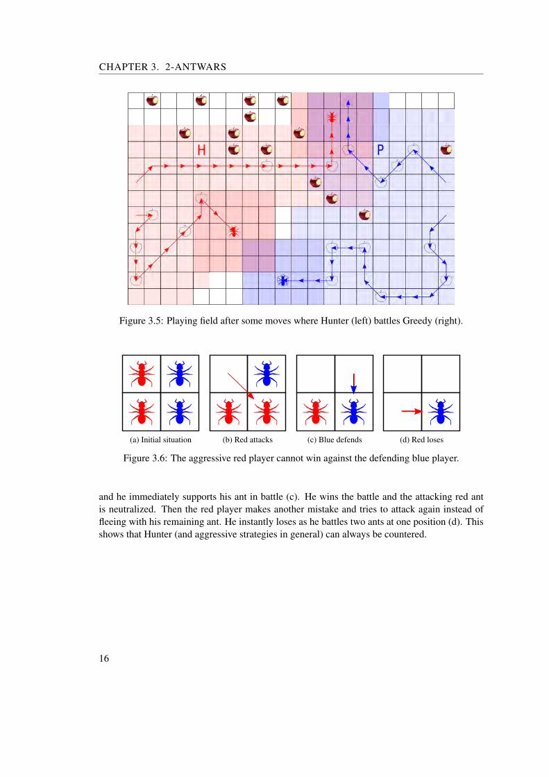
The Hunter strategy is the most aggressive strategy discussed here. It relies on neutralizing oneor even both ants of the opposing player fast, to gain a significant food gathering advantage.Figure 3.5 on the next page shows a game where Hunter (red) and Greedy (blue) battle eachother. The red player used his ant H to hunt the prey P. To gain a speed advantage, he moved Hmore often than his other ant. P tried to flee but ran into the border of the playing field and wasneutralized. The hunt was successful and now the red player has two ants to collect food, whilethe blue player has only one.
This strategy can be countered by any strategy that ensures that the own ants are close enoughto support each other in battle. The rules make certain that when it comes to supporting anant in battle the defending player has a slight advantage because he moves first after a battlestarted. The result of this can be seen in figure 3.6 on the following page. The ants start outas close together as possible to minimize the distance between the place of the battle and thesupporting ant (a). Then the red player decides to attack (b). Now it’s the blue players turn
15
CHAPTER 3. 2-ANTWARS
Figure 3.5: Playing field after some moves where Hunter (left) battles Greedy (right).
(a) Initial situation (b) Red attacks (c) Blue defends (d) Red loses
Figure 3.6: The aggressive red player cannot win against the defending blue player.
and he immediately supports his ant in battle (c). He wins the battle and the attacking red antis neutralized. Then the red player makes another mistake and tries to attack again instead offleeing with his remaining ant. He instantly loses as he battles two ants at one position (d). Thisshows that Hunter (and aggressive strategies in general) can always be countered.
16

Part II
Genetic Programming System


CHAPTER 4Genetic Programming System
This chapter describes the genetic programming system (henceforth called GPS) that was usedto create 2-AntWars players. In a nutshell, it is a compiling typed tree-based (but linearly rep-resented) evolutionary system with memory. The details will be explained in the followingsections. GPS was developed for 2-AntWars but is not bound to it, it can (try to) solve any prob-lem that implements the interface GPS expects. When a problem is mentioned in the followingsections, a problem adhering to the GPS problem interface (like 2-AntWars) is meant. Also,some words will be highlighted, like Function, to emphasise the special meaning they have inthe context of this work. Their meaning will become clear in the course of this chapter.
4.1 The GP-Algorithm
The GP-Algorithm illustrated in listing 4.1 on the next page is the core of GPS. First, the initialPopulation is built and evaluated, then the main loop is entered. Inside of it, a new Population(Pn) is built by selecting the best Individuals from the old Population. Then the crossover opera-tor is applied with the new Population as receiver and a newly selected Population as donor (thisincreases the probability that good Individuals will be crossed with other good Individuals). Seesection 4.6 on page 22 for the semantics of donor and receiver. The new Population is mutated,evaluated and replaces the old Population. Then the cycle begins anew.
4.2 Individual Structure
The central data structure of GPS is the Individual as shown in figure 4.1 on the followingpage. The genetic operators of selection, crossover and mutation work on it to improve theperformance of said Individual. Individuals are stored in the Population and at the lowest levelthey consist of Statements.
Statements are named and modelled after the Statements (and operators) of programminglanguages. Statements have a signature (number and type of arguments, return type) and a
19

CHAPTER 4. GENETIC PROGRAMMING SYSTEM
Population gpProcedure(int maxGen){Population P=initPopulation(); //see 4.4 on page 22evaluatePopulation(P); //see 4.8 on page 24
for(int generation=1;generation<=maxGen;++generation){Population Pn=select(P); //see 4.5 on page 22crossover(Pn,select(P)); //see 4.6 on page 22mutate(Pn); //see 4.7 on page 23evaluatePopulation(Pn);P=Pn;
}return P;
}
Listing 4.1: The GP-Algorithm.
- Score
Individual
Signature
- Name
- Return Type
- Arguments
Body
- Statements
Function
- Name
- Score
FunctionGroup
Signature
- Name
- Return Type
- Arguments
Body
- Statements
Function
...
Signature
- Name
- Return Type
- Arguments
Body
- Statements
Function
- Name
- Score
FunctionGroup
Signature
- Name
- Return Type
- Arguments
Body
- Statements
Function
...
...
Figure 4.1: Structure of GPS Individuals.
name. One example of a Statement might be +: It takes two arguments of type int (the basicC++ integer data type) and returns a value of type int. More specifically it is a FunctionStatementbecause it has arguments. 5 is another Statement. It returns a value of type int (5 according toits name) and has no arguments (which makes it a TerminalStatement).
A Function in GPS is an entity that has a signature and a body. The signature consists of thename of the Function, the return type and the number and types of arguments. The body getsexecuted when the Function is called. Conceptually, the body of a Function is represented astree of Statements (similar to a parse tree). Examples can be found in Figure 4.3 on page 23.The primary difference between a Function and a Statement is that the semantic of a Statement isfixed, that of a Function can be changed by changing its Statement tree. Even though the conceptof a Function is a tree of Statements, it is represented as array in preorder. This representation
20
4.3. POPULATION MODEL
was found to deliver the best speed/size trade-off in [31]. A Function also manages the memoryavailable for the Statements.
A FunctionGroup is a collection of Functions. It has a name and an assigned score thatdescribes the fitness of the set of Functions. A FunctionGroup groups those Functions togetherthat cannot be scored separately. GPS evolves FunctionGroups independently to increase theirfitness.
Finally, an Individual is a collection of FunctionGroups. It has an overall score that describesthe fitness of the combination of FunctionGroups. This score is used to determine the best Indi-vidual inside the Population. GPS assumes that improving the FunctionGroups of an Individualwill result in increased overall fitness.
4.3 Population Model
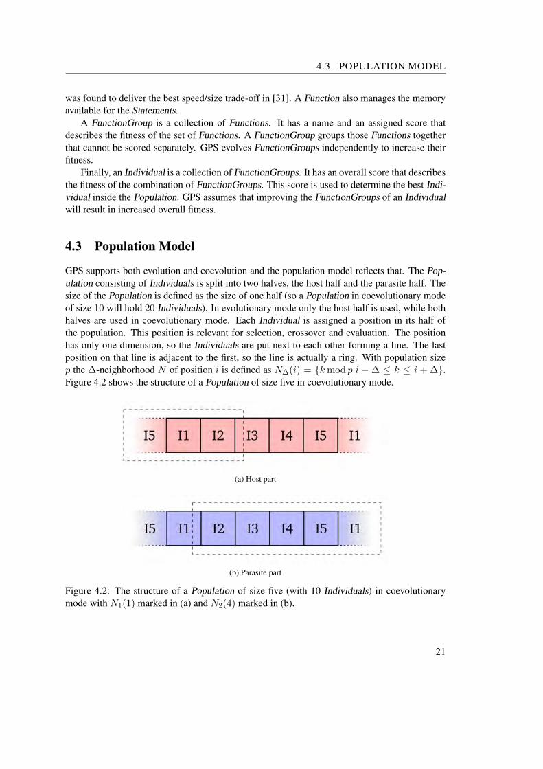
GPS supports both evolution and coevolution and the population model reflects that. The Pop-ulation consisting of Individuals is split into two halves, the host half and the parasite half. Thesize of the Population is defined as the size of one half (so a Population in coevolutionary modeof size 10 will hold 20 Individuals). In evolutionary mode only the host half is used, while bothhalves are used in coevolutionary mode. Each Individual is assigned a position in its half ofthe population. This position is relevant for selection, crossover and evaluation. The positionhas only one dimension, so the Individuals are put next to each other forming a line. The lastposition on that line is adjacent to the first, so the line is actually a ring. With population sizep the ∆-neighborhood N of position i is defined as N∆(i) = {kmod p|i −∆ ≤ k ≤ i + ∆}.Figure 4.2 shows the structure of a Population of size five in coevolutionary mode.
I1
(a) Host part
I1
(b) Parasite part
Figure 4.2: The structure of a Population of size five (with 10 Individuals) in coevolutionarymode with N1(1) marked in (a) and N2(4) marked in (b).
21

CHAPTER 4. GENETIC PROGRAMMING SYSTEM
4.4 Population Initialization
The building blocks of Functions, the Statements, are supplied by the problem. Every Functioncan have a different set of Statements to build its Statement tree out of. The Functions are builtwith the ramped half and half method. The word “ramped” refers to the depth of the trees, whichis uniformly distributed between some minimum and maximum depth. The “half and half” partrefers to the two building algorithms, grow and fill, which each build one half of total amountof Functions. The grow algorithm decides at every depth of the tree and for every argument ofa Statement whether it is supplied by a FunctionStatement or TerminalStatement. If the targetdepth is reached, the growth of the tree is stopped by only using TerminalStatements to supplyarguments. This algorithm results in sparse trees. The grow algorithm always chooses Func-tionStatements to supply arguments unless the target depth is reached. This algorithm resultsin bushy trees. The built Functions are then assembled into FunctionGroups and subsequentlyIndividuals which are placed in the Population.
4.5 Selection
The selection operator works on FunctionGroup level. That means it does not select an Individ-ual based on its score but only a FunctionGroup. GPS tries to increase the performance of anIndividual by increasing the performance of its FunctionGroups. The selection operator uses aform of localized rank selection. When a new FunctionGroup for position i is chosen, the Func-tionGroups at the positions N∆(i) (with the set selection-delta) are sorted according to theirfitness. The sorted FunctionGroups are traversed from best to worst fitness until a Function-Group is selected. During the traversal, each FunctionGroup has a chance of 50% to be selected.If no FunctionGroup is selected during the traversal, the worst FunctionGroup is selected.
4.6 Crossover
The crossover operator works as one would expect for genetic programming. A sub-tree ofStatements of a Function (donor) is copied and inserted in another Function (receiver). GPSensures that the return types of the root Statement of the copied sub-tree and the sub-tree thatis replaced in the receiver are equivalent (automatic type conversion is not supported). Sinceselection works on FunctionGroup level but crossover works on Functions the crossover operatorhas the additional task to select which Functions are actually crossed. To do so, the operator isgiven the selected donor and receiver FunctionGroups. Then it iterates over the Functions of thereceiving FunctionGroup. Every Function has a probability of pc to be actually used as receiver.If a Function is used as one, a compatible Function in the donor is selected. Neither does ithave to be the same Function nor a Function in the same FunctionGroup. The problem specifieswhich receiver-donor pairs are compatible. If the result of the crossover is bigger than the setlimit for the Function, the original receiver is kept.
22
4.7. MUTATION
+
3 -
1 7
(a) Initial
+
3 *
- 2
1 7
(b) Grow
+
3 7
(c) Shrink
+
3 *
1 7
(d) Inplace
+
3 /
5 8
(e) Replace
Figure 4.3: The effect of the four different types of mutation available in GPS.
4.7 Mutation
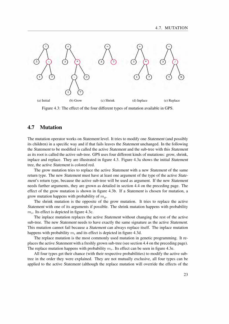
The mutation operator works on Statement level. It tries to modify one Statement (and possiblyits children) in a specific way and if that fails leaves the Statement unchanged. In the followingthe Statement to be modified is called the active Statement and the sub-tree with this Statementas its root is called the active sub-tree. GPS uses four different kinds of mutations: grow, shrink,inplace and replace. They are illustrated in figure 4.3. Figure 4.3a shows the initial Statementtree, the active Statement is colored red.
The grow mutation tries to replace the active Statement with a new Statement of the samereturn type. The new Statement must have at least one argument of the type of the active State-ment’s return type, because the active sub-tree will be used as argument. If the new Statementneeds further arguments, they are grown as detailed in section 4.4 on the preceding page. Theeffect of the grow mutation is shown in figure 4.3b. If a Statement is chosen for mutation, agrow mutation happens with probability of mg.
The shrink mutation is the opposite of the grow mutation. It tries to replace the activeStatement with one of its arguments if possible. The shrink mutation happens with probabilityms. Its effect is depicted in figure 4.3c.
The inplace mutation replaces the active Statement without changing the rest of the activesub-tree. The new Statement needs to have exactly the same signature as the active Statement.This mutation cannot fail because a Statement can always replace itself. The inplace mutationhappens with probability mi and its effect is depicted in figure 4.3d.
The replace mutation is the most commonly used mutation in genetic programming. It re-places the active Statement with a freshly grown sub-tree (see section 4.4 on the preceding page).The replace mutation happens with probability mr. Its effect can be seen in figure 4.3e.
All four types get their chance (with their respective probabilities) to modify the active sub-tree in the order they were explained. They are not mutually exclusive, all four types can beapplied to the active Statement (although the replace mutation will override the effects of the
23

CHAPTER 4. GENETIC PROGRAMMING SYSTEM
other mutations) or even none may be applied. The red markings in figure 4.3 on the previouspage show which Statements are active after a mutation.
A part of the mutation operator works on Function level. It decides how many places inthe Statement tree are mutated. The probability of a Statement to undergo mutation is pm. APoisson distributed random variable (depending on pm and the size of the Statement tree) isused to calculate how many Statements will be chosen randomly for mutation. If the result ofthe mutation is bigger that the set limit for the Function, the original is kept.
4.8 Evaluation
The job of the evaluation is to assign a score to each Individual in the Population. The first stepis to transform the Functions of the Individuals into executable code. Every Statement has afunction that allows to print it in a compilable way. During the construction of the source codefile, this function is called before any of the Statement’s children have been printed and aftereach printed child. An if-Statement for instance will print “if(” before its arguments are printed,“){” after the first argument (the condition) and “}” after the second argument (the body). Thesource code is then split into parts, each containing only a fraction of the code generated fromthe Population. This has two advantages. First of all, the code can be compiled in parallel whichspeeds up the process immensely because every code fragment is completely independent fromall other fragments. Secondly, the code can be compiled serially in smaller chunks which keepsthe total amount of needed memory low. Which way (or combination) is preferable depends oncompilation flags (aggressive optimization needs more memory), the Individual structure of theproblem GPS has to solve and of course the available memory. To provide a frame of reference,for the 2-AntWars problem the typical code size was 10MB with 200000 lines of code. It wascompiled in two chunks without optimization (-O0) and each compiler instance needed about500MB of memory. After the compilation, the object files are linked to form a dynamicallyloadable library. This library is loaded by GPS and the function pointers for the Functions areextracted.
Now the actual evaluation can start. The mode of evaluation depends on whether evolutionor coevolution is performed. In the case of evolution, the problem is given a set of Functions ac-cording to the Individual-structure. The problem calculates the scores (for each FunctionGroupand the total score) and returns them to GPS, which assigns them to the Individual. The coevo-lutionary case is a bit more complex. First of all, the problem gets two sets of functions (onefrom an Individual in the host half and one from an Individual in the parasite half) and returnsthe score. Normally, the Individuals that are evaluated have the same position in their respectivehalves of the population. GPS also allows asymmetric evaluation, where a host Individual isevaluated multiple times with a ∆-neighborhood centered around the parasite that is used fornormal evaluation. While the parasite is only assigned the score of the evaluation with the hostat the same position, the host is assigned the combination of scores of all evaluations. How thescores are combined depends on the problem as it provides the particular score to use.
24

CHAPTER 5Modelling the 2-AntWars Player
The model of the 2-AntWars player is based on the successful model for AntWars presented in[32]. It consists of four FunctionGroups: movement, belief, predict1 and predict2.
The movement FunctionGroup is concerned with deciding which ant should move in whichdirection. To that effect, it consists of three Functions: decision, movement1 and movement2.The movement1 and movement2 Functions each calculate the movement of one ant and the de-cision Function decides which ant moves in the end. The score of the movement FunctionGroupis based on the food the player is able to gather during a 2-AntWars match. This is a good ex-ample of Functions that cannot be individually scored. It is not known which decision Functionbehaviour is advantageous and should be rewarded. Only in combination with the movementFunction a score can be assigned.
The belief FunctionGroup consists of the belief Function. Belief in food was introduced in[32]. Ants have only a very limited view of the playing field. To support the calculation of thenext move, they remember food they have seen previously (but do not see now). However, itis not certain that the food that has been seen is still there (the other player might have eatenit), hence the food belief. It is a measure of how certain a player is that a position still containsfood (or that a never seen field contains food). In [32] the belief was fixed by the program.After every move it would be reduced to a fraction of its old value. It is not clear that this isthe optimal method. The 2-AntWars model includes an evolvable belief Function to find a goodway to calculate the belief, without any preconceptions. The belief FunctionGroup is scored bycalculating the deviation between belief and reality in the following way, given position p andbelief b: If p has already been seen, 1− b is added to the belief deviation if p contains food, b isadded otherwise. If p has not been seen and it contains food 1− b is added. Otherwise nothingis added which means believing in food at unseen positions does not contribute to the deviation.This calculation is carried out for every position after every move and the sum of all deviationsgives the final score (in this case a lower score is better). As can be seen from the deviationcalculation, belief is expected to be ∈ [0, 1]. This is not enforced by the model, evolution hasto figure it out. What is enforced, however, is that positions that are currently seen always have
25

CHAPTER 5. MODELLING THE 2-ANTWARS PLAYER
the correct food belief assigned (zero if there is no food, one if there is food), so the player canchange how he believes in his memory but has to believe his eyes.
The predict1 and predict2 FunctionGroups each contain one Function with the same name.Their task is to predict the position of the enemy’s ants. After every move, the distance (inmoves) between the prediction and the corresponding ant is calculated. The sum of the distancesduring a match constitutes the score of the two predict FunctionGroups.
So to sum it up, a 2-AntWars player consists of six Functions: belief, decision, movement1,movement2, predict1 and predict2. Listing 5.1 on the facing page gives an overview on how theFunctions are used to decide which ant to move. They (and the Statements that are availablefor them) are discussed in detail in the following sections after the basic data types have beenintroduced. All the scores use the size of the function as secondary criterion to decide whichscore is better. For instance, when two movement FunctionGroups find the same amount offood the smaller one is better. This introduces selective pressure towards parsimonious solu-tions and more so in later generations when the probability of FunctionGroups having the sameperformance rises.
5.1 Data Types
The data types of Statements (their return type and argument types) are used to decide whichones are compatible. 2-AntWars uses the following custom data types:
AntID: The ID of an ant. It can be zero or one and is returned by the decision function toindicate which ant has to be moved.
Ant: The state of an ant. It contains among other things information about the position of theant and the amount of moves it has left.
Direction: A single direction, like north (N) or south-west (SW).
Moves: This data type stores a subset of the possible movement directions of an ant. For in-stance, a variable of type moves may contain the Directions NW, W and S. Set arithmetic(union, intersection etc.) is possible with variables of type Moves.
Position: A position on the playing field. A Position can be moved by adding a Direction, butit will always stay valid (i.e. on the playing field).
PositionPredictionInfo: A data structure containing information about the prediction of an en-emy ant. It contains the time and position of the last sighting of the enemy ant and thecurrent prediction of the position of the ant. The information whether the ant was seenmovable is also recorded. At the begin of the game it is initialized with the starting posi-tion of the ant that is predicted.
PlayerState: The complete state of a player. It contains information about his ants, what theyare currently seeing, what positions they have seen, how much food the player has eatenand all positions where he has seen food and what the food belief for every position onthe playing field is.
26
5.1. DATA TYPES
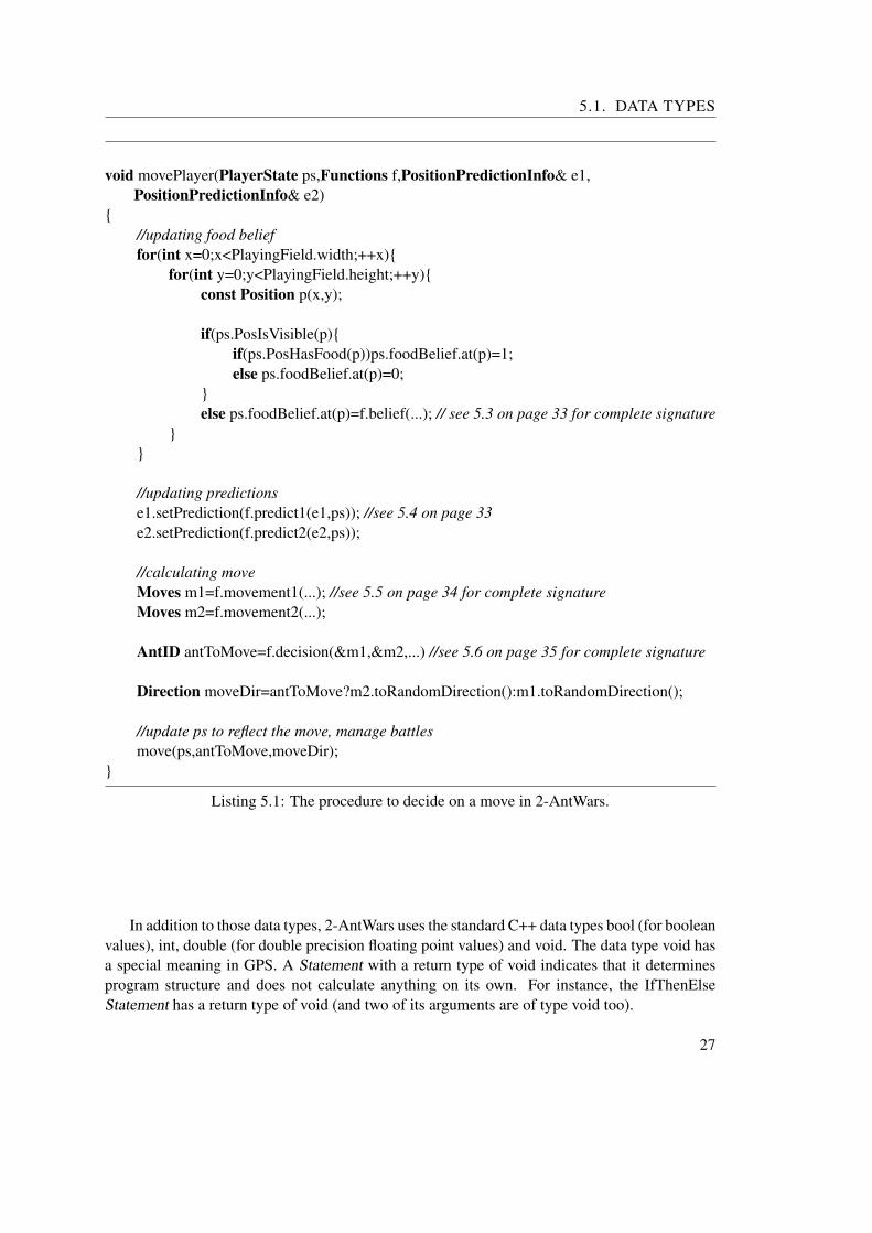
void movePlayer(PlayerState ps,Functions f,PositionPredictionInfo& e1,PositionPredictionInfo& e2)
{//updating food belieffor(int x=0;x<PlayingField.width;++x){
for(int y=0;y<PlayingField.height;++y){const Position p(x,y);
if(ps.PosIsVisible(p){if(ps.PosHasFood(p))ps.foodBelief.at(p)=1;else ps.foodBelief.at(p)=0;
}else ps.foodBelief.at(p)=f.belief(...); // see 5.3 on page 33 for complete signature
}}
//updating predictionse1.setPrediction(f.predict1(e1,ps)); //see 5.4 on page 33e2.setPrediction(f.predict2(e2,ps));
//calculating moveMoves m1=f.movement1(...); //see 5.5 on page 34 for complete signatureMoves m2=f.movement2(...);
AntID antToMove=f.decision(&m1,&m2,...) //see 5.6 on page 35 for complete signature
Direction moveDir=antToMove?m2.toRandomDirection():m1.toRandomDirection();
//update ps to reflect the move, manage battlesmove(ps,antToMove,moveDir);
}
Listing 5.1: The procedure to decide on a move in 2-AntWars.
In addition to those data types, 2-AntWars uses the standard C++ data types bool (for booleanvalues), int, double (for double precision floating point values) and void. The data type void hasa special meaning in GPS. A Statement with a return type of void indicates that it determinesprogram structure and does not calculate anything on its own. For instance, the IfThenElseStatement has a return type of void (and two of its arguments are of type void too).
27
CHAPTER 5. MODELLING THE 2-ANTWARS PLAYER
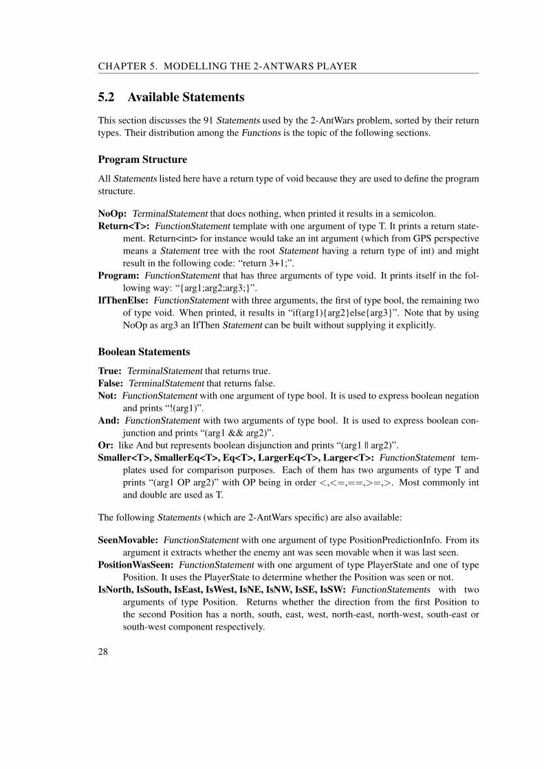
5.2 Available Statements
This section discusses the 91 Statements used by the 2-AntWars problem, sorted by their returntypes. Their distribution among the Functions is the topic of the following sections.
Program Structure
All Statements listed here have a return type of void because they are used to define the programstructure.
NoOp: TerminalStatement that does nothing, when printed it results in a semicolon.Return<T>: FunctionStatement template with one argument of type T. It prints a return state-
ment. Return<int> for instance would take an int argument (which from GPS perspectivemeans a Statement tree with the root Statement having a return type of int) and mightresult in the following code: “return 3+1;”.
Program: FunctionStatement that has three arguments of type void. It prints itself in the fol-lowing way: “{arg1;arg2;arg3;}”.
IfThenElse: FunctionStatement with three arguments, the first of type bool, the remaining twoof type void. When printed, it results in “if(arg1){arg2}else{arg3}”. Note that by usingNoOp as arg3 an IfThen Statement can be built without supplying it explicitly.
Boolean Statements
True: TerminalStatement that returns true.False: TerminalStatement that returns false.Not: FunctionStatement with one argument of type bool. It is used to express boolean negation
and prints “!(arg1)”.And: FunctionStatement with two arguments of type bool. It is used to express boolean con-
junction and prints “(arg1 && arg2)”.Or: like And but represents boolean disjunction and prints “(arg1 || arg2)”.Smaller<T>, SmallerEq<T>, Eq<T>, LargerEq<T>, Larger<T>: FunctionStatement tem-
plates used for comparison purposes. Each of them has two arguments of type T andprints “(arg1 OP arg2)” with OP being in order <,<=,==,>=,>. Most commonly intand double are used as T.
The following Statements (which are 2-AntWars specific) are also available:
SeenMovable: FunctionStatement with one argument of type PositionPredictionInfo. From itsargument it extracts whether the enemy ant was seen movable when it was last seen.
PositionWasSeen: FunctionStatement with one argument of type PlayerState and one of typePosition. It uses the PlayerState to determine whether the Position was seen or not.
IsNorth, IsSouth, IsEast, IsWest, IsNE, IsNW, IsSE, IsSW: FunctionStatements with twoarguments of type Position. Returns whether the direction from the first Position tothe second Position has a north, south, east, west, north-east, north-west, south-east orsouth-west component respectively.
28

5.2. AVAILABLE STATEMENTS
AntIsMovable: FunctionStatement that returns true if the Ant supplied as argument is movable(i.e. has moves left and is not in battle or neutralized).
AntIsPassive: FunctionStatement with one argument of type Ant that returns true if the Antcannot move or interact with anything (i.e. is neutralized).
AntInBattle: FunctionStatement that returns true if the supplied Ant argument is currently en-gaged in battle.
Integer Statements
EpInt(min,max,delta): ephemeral constant with a value ∈ [min,max]. This Statement usesa custom mutation operator, i.e. it does not use the methods outlined in section 4.7 onpage 23. Instead, it adds a uniformly distributed value ∈ [−delta, delta] to the currentvalue (while respecting min and max).
AddI, SubI, ModI: FunctionStatements that facilitate addition, subtraction and modulo divi-sion. They each have two arguments of type int and print “(arg1 OP arg2)” with OP being+,− and %. Note that modulo division is protected and returns the value of arg1 if arg2equals zero.
In addition to these general purpose Statements, the following Statements specific to 2-AntWarsare available:
Width, Height: TerminalStatements that return the width (20) and height (13) of the playingfield respectively.
TotalFood: TerminalStatement that returns the total amount of food available on the playingfield (32).
MovesPerAnt: TerminalStatement that returns the total amount of moves that an ant is allowedto make (40).
BattleRounds: TerminalStatement that returns the number of battle rounds before the battle isfinished (5).
PosGetX, PosGetY: FunctionStatements with one argument of type Position. They extract theX and Y coordinates of their argument.
DistanceMoves: FunctionStatement with two arguments of type Position that returns the dis-tance in moves between those Positions.
ElapsedTime: FunctionStatement that extracts the elapsed time (which equals the number ofmoves made by a player) from its argument of type PlayerState.
FoundFood: FunctionStatement with one argument of type PlayerState. It returns the amountof food the player has already found.
SightingTime: FunctionStatement with one argument of typePlayerState and one argument oftype Position. It uses the PlayerState to return the last time the Position was seen. If thePosition was never seen, it returns zero.
AntExtractX, AntExtractY: FunctionStatement with one argument of type Ant. It extracts theX (or Y) component of the Ant’s position.
AntMovesLeft: FunctionStatement with one argument of type Ant. It extracts the number ofmoves the Ant has left.
29

CHAPTER 5. MODELLING THE 2-ANTWARS PLAYER
TimeOfLastSighting: FunctionStatement that extracts the time of last sighting from its argu-ment of type PositionPredictionInfo.
Double Statements
AddD, SubD, MulD, DivD: FunctionStatements that facilitate addition, subtraction, multipli-cation and division. They each have two arguments of type double and print “(arg1 OParg2)” with OP being in order +,−,∗ and /. Note that DivD is not protected and divisionby zero will be executed. This results in the value mandated by IEEE 754 floating pointarithmetic rules (i.e. NaN or ± INF depending on the divisor).
Sin, Cos: FunctionStatements for trigonometric functions, each taking one argument of typedouble.
Pow: FunctionStatement with two arguments of type double. Returns the result of arg1arg2.Log: FunctionStatement with one argument of type double. Returns the natural logarithm of
arg1.EpDouble(µ,σ): an ephemeral constant with value µ. This Statement uses a custom mutation
operator, i.e. it does not use the methods outlined in section 4.7 on page 23. Instead, ituses an N(0, σ) distributed random variable to offset its µ.
EpDoubleRange(µ,σ,min,max): an ephemeral constant like EpDouble but with a value guar-anteed to be ∈ [min,max].
The following Statements are specific to the 2-AntWars context:
PositionDistance: FunctionStatement with two arguments of type Position. It returns the eu-clidean distance between them.
FoodBeliefAtPos: FunctionStatement with one argument of type PlayerState and one of Posi-tion. It returns the food belief at the passed Position on the playing field.
Position Statements
PosPlusDirection: FunctionStatement with one argument of type Position and one argument oftype Direction. It returns a Position moved in Direction. If the Position would leave theplaying field it is not changed.
PosPlusCoordinates: FunctionStatement with one argument of type Position and two argu-ments of type int. It returns a Position with the int arguments added to the x- and y-coordinates of the Position argument. The coordinates are clamped to the borders of theplaying field so the resulting Position is always valid.
CurrentPrediction: FunctionStatement with one argument of type PositionPredictionInfo. Itextracts the current predicted position.
LastSeenPosition: Like CurrentPrediction, but extracts the last seen position from its argument.AntPosition: FunctionStatement that extracts the position of its one argument of type Ant.EpPosition(δ): an ephemeral constant of type Position. It is initialized with a random Position
on the playing field. The custom mutation operator offsets the coordinates of the Posi-tion with a uniformly distributed random value in the range of ±δ (while ensuring validcoordinate values).
30

5.2. AVAILABLE STATEMENTS
NearestFood: FunctionStatement with four arguments, one of type PlayerState, one Position p,one double b and one integer n. This Statement sorts the Positions with a food belief notsmaller than b by their distance in moves to p. If there is no such Position, p is returned.Otherwise the Statement returns the n-th nearest Position, with counting starting at zero.If n is smaller then zero, zero is assumed. If there is no n-th nearest Position, the Positionwith the largest distance is returned.
NearestUnseenField: FunctionStatement with three arguments, one of type PlayerState, onePosition p and one integer n. It works like NearestFood, but Positions qualify if they havenot been seen, not because of their assigned food belief.
Direction Statement
2-AntWars has only one Statement that returns a type of Direction (disregarding constants).The Statement is called ToRandomDirection. It is a FunctionStatement that returns a randomDirection from its argument of type Moves.
Moves Statements
MNone: TerminalStatement returning a Moves value without any movement directions set.MAll: TerminalStatement returning a Moves value with all movement directions set.MToward, MNeutral, MAway: FunctionStatements with two arguments of type Position and
calculating Moves that will decrease, not change or increase the distance (in number ofmoves) between its two arguments when applied to the first argument.
MIntersection, MUnion, MDifference: FunctionStatements with two arguments of typeMoves and returning the result of the corresponding set operation.
MNot: FunctionStatement that inverts its argument of type Move. The return value will containall Directions the argument does not.
MAddDirection, MSubDirection: FunctionStatements with one argument of type Moves andone of type Direction evaluating to a Moves value with the Direction argument added to(or removed from) the Moves argument.
FoodEatMoves: FunctionStatement with one argument of type PlayerState and one argumentof type Position. It checks for which of the (at most) eight neighboring Positions of thePosition argument the food belief is above zero and returns a Moves value containing thedirections from the Position argument to those Positions.
FoodEatMovesMaxBelief: FunctionStatement like FoodEatMoves, but instead returns all Di-rections with the maximum belief.
FoodEatMovesAboveBelief: FunctionStatement like FoodEatMoves, but with one additionalargument of type double. It will only add directions to positions to the return value if theposition’s food belief is not smaller than the double argument.
MaxNewFieldsMoves: FunctionStatement with one argument of type Position and one argu-ment of type PlayerState. It returns all the movement directions from its Position argumentthat achieve the maximum of newly seen fields.
NearestFoodMoves: FunctionStatement with four arguments, one of type PlayerState, a Posi-tion p, a double b and an integer n. This Statement takes all Positions on the playing field
31
CHAPTER 5. MODELLING THE 2-ANTWARS PLAYER
with a food belief not smaller than b and sorts them by distance (in number of moves) top. If no Positions qualify, then an empty Moves value is returned. From all qualifyingPositions, only those on the n-th distance level are regarded (counting starts at zero). Ifn is smaller than zero, the zero-th level is used. If n is larger than the total number ofdistance levels, the level with the highest distance is used. The Statement then returnsa Moves value with all Directions from p to the Positions on the target distance level.This is the most powerful Statement available to 2-AntWars as it transforms the seen food(more precisely the food belief) into useful Moves without the need to evolve loops ordata structures.
NearestUnseenFieldMoves: FunctionStatement with three arguments, one of type PlayerState,a Position p and an integer n. This Statement works like NearestFoodMoves, but Positionsqualify if they have not been seen yet and not because of food belief.
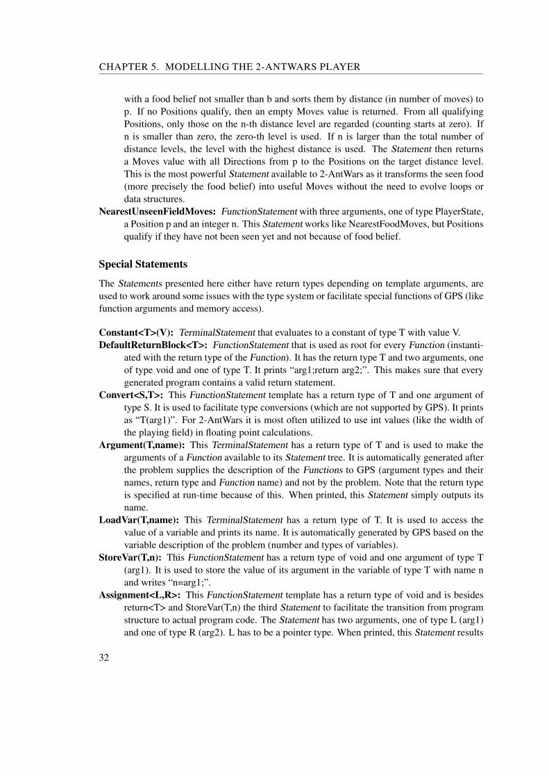
Special Statements
The Statements presented here either have return types depending on template arguments, areused to work around some issues with the type system or facilitate special functions of GPS (likefunction arguments and memory access).
Constant<T>(V): TerminalStatement that evaluates to a constant of type T with value V.DefaultReturnBlock<T>: FunctionStatement that is used as root for every Function (instanti-
ated with the return type of the Function). It has the return type T and two arguments, oneof type void and one of type T. It prints “arg1;return arg2;”. This makes sure that everygenerated program contains a valid return statement.
Convert<S,T>: This FunctionStatement template has a return type of T and one argument oftype S. It is used to facilitate type conversions (which are not supported by GPS). It printsas “T(arg1)”. For 2-AntWars it is most often utilized to use int values (like the width ofthe playing field) in floating point calculations.
Argument(T,name): This TerminalStatement has a return type of T and is used to make thearguments of a Function available to its Statement tree. It is automatically generated afterthe problem supplies the description of the Functions to GPS (argument types and theirnames, return type and Function name) and not by the problem. Note that the return typeis specified at run-time because of this. When printed, this Statement simply outputs itsname.
LoadVar(T,name): This TerminalStatement has a return type of T. It is used to access thevalue of a variable and prints its name. It is automatically generated by GPS based on thevariable description of the problem (number and types of variables).
StoreVar(T,n): This FunctionStatement has a return type of void and one argument of type T(arg1). It is used to store the value of its argument in the variable of type T with name nand writes “n=arg1;”.
Assignment<L,R>: This FunctionStatement template has a return type of void and is besidesreturn<T> and StoreVar(T,n) the third Statement to facilitate the transition from programstructure to actual program code. The Statement has two arguments, one of type L (arg1)and one of type R (arg2). L has to be a pointer type. When printed, this Statement results
32

5.3. BELIEF FUNCTION
double belief(Position p, bool haveSeenField, bool haveSeenFood, int timeSinceSighting, intelapsedTime, int foundFood, int seenFields, PositionPredictionInfo enemy1,PositionPredictionInfo enemy2);
Listing 5.2: The signature of the belief function.
Position predict(PositionPredictionInfo ppi, PlayerState ps);
Listing 5.3: The signature of the predict functions.
in “(*arg1)=arg2;”. It has to be ensured that this assignment makes sense from the pointof view of the C++ type system. For an usage example, see section 5.6 on page 35.
5.3 Belief Function
This section describes the signature of the belief Function and lists the available Statements forit. The signature is shown in listing 5.2 and the meaning of its arguments is described below:
p: Position for which the belief is being calculatedhaveSeenField: true if the position has been seenhaveSeenFood: true if the position contained food when it was last seentimeSinceSighting: number of moves since the position was seenelapsedTime: number of moves since the start of the gamefoundFood: number of food the player has already eatenseenFields: number of fields that have been seen at least onceenemy1, enemy2: prediction information for the ants of the enemy
The following Statements are available for the belief Function:
void: NoOp, IfThenElse, Program, Return<double>bool: True, Not, And, Or, SmallerEq<double>, LargerEq<double>, SeenMovableint: Width, Height, TotalFood, PosGetX, PosGetY, TimeOfLastSighting, DistanceMovesdouble: EpDouble(0.5,0.15), Sin, Cos, Log, Pow, AddD, SubD, MulD, DivDPosition: CurrentPrediction, LastSeenPositionSpecial: DefaultReturnBlock<double>, Convert<int,double>, Constant<double>(0), Con-
stant<double>(1)
The belief Function has no variables and is only to itself crossover compatible.
5.4 Predict Functions
This section describes the signature of the predict Functions and lists the available Statementsfor it. The signature is shown in listing 5.3 and its arguments are described below:
33
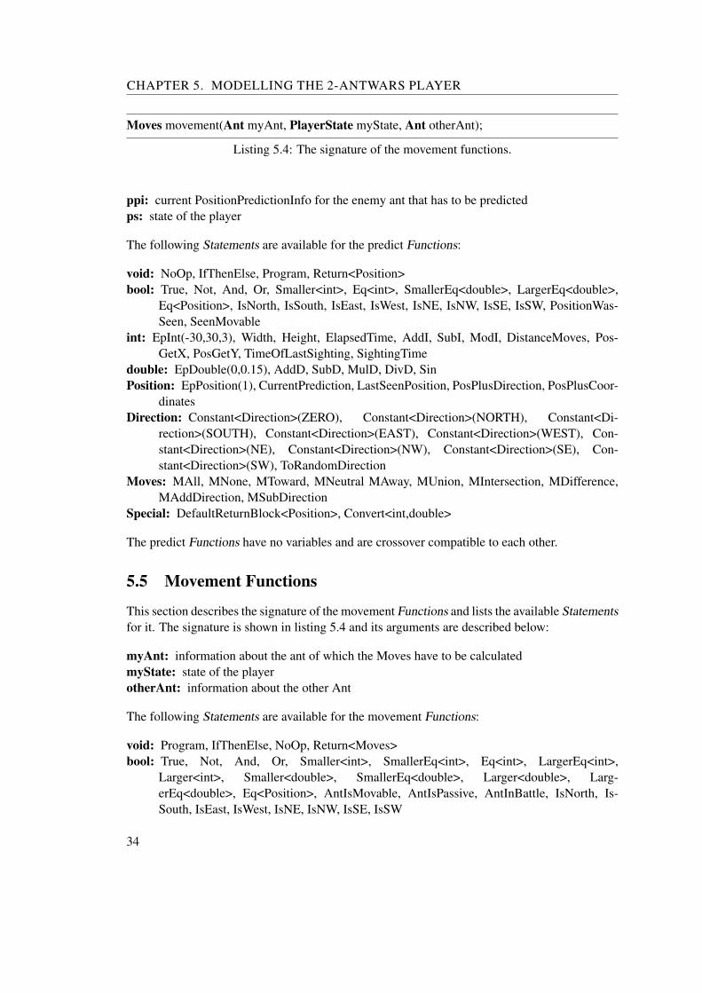
CHAPTER 5. MODELLING THE 2-ANTWARS PLAYER
Moves movement(Ant myAnt, PlayerState myState, Ant otherAnt);
Listing 5.4: The signature of the movement functions.
ppi: current PositionPredictionInfo for the enemy ant that has to be predictedps: state of the player
The following Statements are available for the predict Functions:
void: NoOp, IfThenElse, Program, Return<Position>bool: True, Not, And, Or, Smaller<int>, Eq<int>, SmallerEq<double>, LargerEq<double>,
Eq<Position>, IsNorth, IsSouth, IsEast, IsWest, IsNE, IsNW, IsSE, IsSW, PositionWas-Seen, SeenMovable
int: EpInt(-30,30,3), Width, Height, ElapsedTime, AddI, SubI, ModI, DistanceMoves, Pos-GetX, PosGetY, TimeOfLastSighting, SightingTime
double: EpDouble(0,0.15), AddD, SubD, MulD, DivD, SinPosition: EpPosition(1), CurrentPrediction, LastSeenPosition, PosPlusDirection, PosPlusCoor-
dinatesDirection: Constant<Direction>(ZERO), Constant<Direction>(NORTH), Constant<Di-
rection>(SOUTH), Constant<Direction>(EAST), Constant<Direction>(WEST), Con-stant<Direction>(NE), Constant<Direction>(NW), Constant<Direction>(SE), Con-stant<Direction>(SW), ToRandomDirection
Moves: MAll, MNone, MToward, MNeutral MAway, MUnion, MIntersection, MDifference,MAddDirection, MSubDirection
Special: DefaultReturnBlock<Position>, Convert<int,double>
The predict Functions have no variables and are crossover compatible to each other.
5.5 Movement Functions
This section describes the signature of the movement Functions and lists the available Statementsfor it. The signature is shown in listing 5.4 and its arguments are described below:
myAnt: information about the ant of which the Moves have to be calculatedmyState: state of the playerotherAnt: information about the other Ant
The following Statements are available for the movement Functions:
void: Program, IfThenElse, NoOp, Return<Moves>bool: True, Not, And, Or, Smaller<int>, SmallerEq<int>, Eq<int>, LargerEq<int>,
Larger<int>, Smaller<double>, SmallerEq<double>, Larger<double>, Larg-erEq<double>, Eq<Position>, AntIsMovable, AntIsPassive, AntInBattle, IsNorth, Is-South, IsEast, IsWest, IsNE, IsNW, IsSE, IsSW
34

5.6. DECISION FUNCTION
AntID decision(Moves∗ m1, Moves∗ m2, Ant a1, Ant a2, PositionPredictionInfo enemy1,PositionPredictionInfo enemy2, PlayerState ps, int battleEndTime);
Listing 5.5: The signature of the decision function.
int: EpInt(0,20,2), AddI, SubI, Width, Height, MovesPerAnt, TotalFood, BattleRounds, Ant-ExtractX, AntExtractY, AntMovesLeft, PosGetX, PosGetY, ElapsedTime, FoundFood,DistanceMoves
double: EpDouble(0.5,0.15), FoodBeliefAtPos, PositionDistancePosition: EpPosition(1), AntPosition, NearestFood, NearestUnseenFieldDirection: Constant<Direction>(NORTH), Constant<Direction>(SOUTH), Constant<Direc-
tion>(EAST), Constant<Direction>(WEST), Constant<Direction>(NE), Con-stant<Direction>(NW), Constant<Direction>(SE), Constant<Direction>(SW)
Moves: MAll, MNone, MToward, MNeutral, MAway, MUnion, MIntersection, MDif-ference, MNot, Constant<Moves>(NORTH), Constant<Moves>(SOUTH), Con-stant<Moves>(EAST), Constant<Moves>(WEST), Constant<Moves>(NE), Con-stant<Moves>(NW), Constant<Moves>(SE), Constant<Moves>(SW), FoodEatMoves,FoodEatMovesMaxBelief, FoodEatMovesAboveBelief, MaxNewFieldsMoves, Nearest-FoodMoves, NearestUnseenFieldMoves, MAddDirection, MSubDirection, PosPlusDi-rection
Special: DefaultReturnBlock<Moves>
The movement functions have access to two variables of type Position, Direction and Moves andare crossover compatible to each other.
5.6 Decision Function
This section describes the signature of the decision Function and lists the available Statementsfor it. The signature is shown in listing 5.5 and its arguments are described below:
m1, m2: Moves suggested by the movement functions. They are pointers because the decisionfunction can change them.
a1, a2: Ants of the player.enemy1, enemy2: PositionPredictionInfo about the enemy ants.ps: State of the player.battleEndTime: End time of a battle if such a battle exists. If none is being fought, the current
time is passed as argument. If two battles are being fought simultaneously, the argumentis the end time of one of those battles. Which one is unspecified because there are nomovable ants in such a case.
35
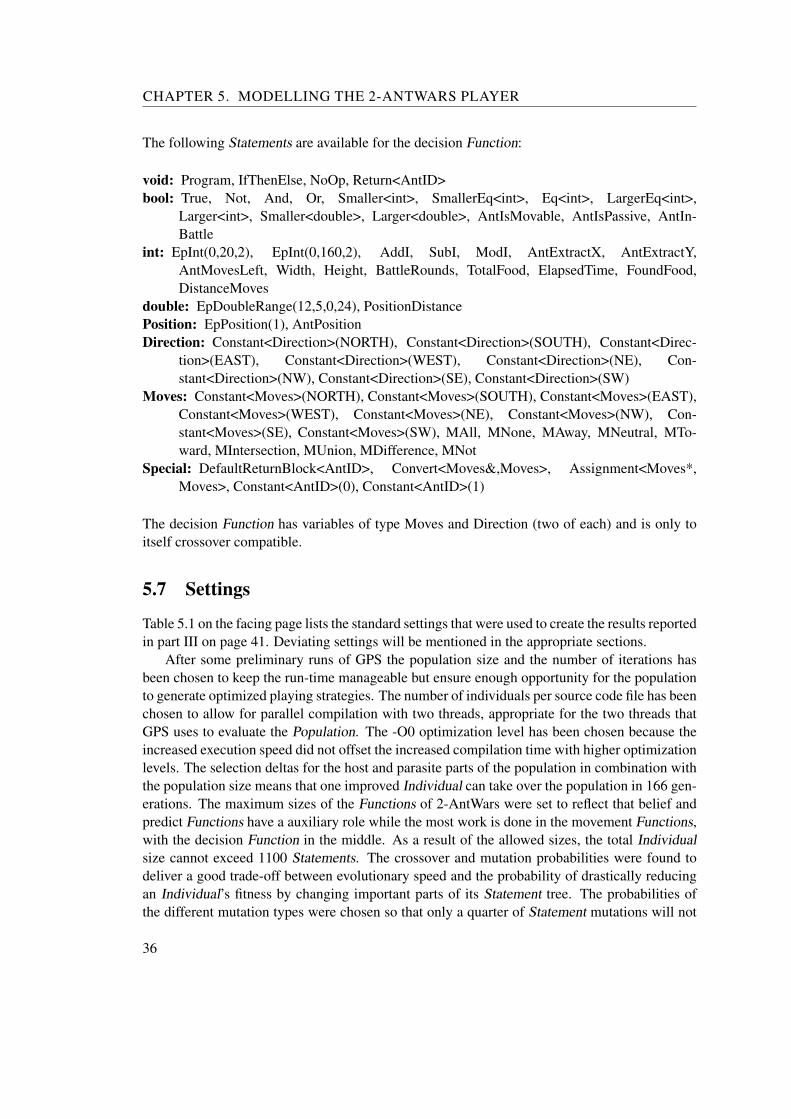
CHAPTER 5. MODELLING THE 2-ANTWARS PLAYER
The following Statements are available for the decision Function:
void: Program, IfThenElse, NoOp, Return<AntID>bool: True, Not, And, Or, Smaller<int>, SmallerEq<int>, Eq<int>, LargerEq<int>,
Larger<int>, Smaller<double>, Larger<double>, AntIsMovable, AntIsPassive, AntIn-Battle
int: EpInt(0,20,2), EpInt(0,160,2), AddI, SubI, ModI, AntExtractX, AntExtractY,AntMovesLeft, Width, Height, BattleRounds, TotalFood, ElapsedTime, FoundFood,DistanceMoves
double: EpDoubleRange(12,5,0,24), PositionDistancePosition: EpPosition(1), AntPositionDirection: Constant<Direction>(NORTH), Constant<Direction>(SOUTH), Constant<Direc-
tion>(EAST), Constant<Direction>(WEST), Constant<Direction>(NE), Con-stant<Direction>(NW), Constant<Direction>(SE), Constant<Direction>(SW)
Moves: Constant<Moves>(NORTH), Constant<Moves>(SOUTH), Constant<Moves>(EAST),Constant<Moves>(WEST), Constant<Moves>(NE), Constant<Moves>(NW), Con-stant<Moves>(SE), Constant<Moves>(SW), MAll, MNone, MAway, MNeutral, MTo-ward, MIntersection, MUnion, MDifference, MNot
Special: DefaultReturnBlock<AntID>, Convert<Moves&,Moves>, Assignment<Moves*,Moves>, Constant<AntID>(0), Constant<AntID>(1)
The decision Function has variables of type Moves and Direction (two of each) and is only toitself crossover compatible.
5.7 Settings
Table 5.1 on the facing page lists the standard settings that were used to create the results reportedin part III on page 41. Deviating settings will be mentioned in the appropriate sections.
After some preliminary runs of GPS the population size and the number of iterations hasbeen chosen to keep the run-time manageable but ensure enough opportunity for the populationto generate optimized playing strategies. The number of individuals per source code file has beenchosen to allow for parallel compilation with two threads, appropriate for the two threads thatGPS uses to evaluate the Population. The -O0 optimization level has been chosen because theincreased execution speed did not offset the increased compilation time with higher optimizationlevels. The selection deltas for the host and parasite parts of the population in combination withthe population size means that one improved Individual can take over the population in 166 gen-erations. The maximum sizes of the Functions of 2-AntWars were set to reflect that belief andpredict Functions have a auxiliary role while the most work is done in the movement Functions,with the decision Function in the middle. As a result of the allowed sizes, the total Individualsize cannot exceed 1100 Statements. The crossover and mutation probabilities were found todeliver a good trade-off between evolutionary speed and the probability of drastically reducingan Individual’s fitness by changing important parts of its Statement tree. The probabilities ofthe different mutation types were chosen so that only a quarter of Statement mutations will not
36

5.7. SETTINGS
result in any change. It is important to note that the minimum depth of the Statement trees isthe real minimum, Statement trees cannot be smaller. The root Statement is always a Default-ReturnBlock, its argument of type void can be filled by a Return Statement which in turn needsat least a TerminalStatement as argument, so the total depth of the tree is two.
Table 5.1: Default GPS settings for the 2-AntWars problem.
Setting Name Description ValuePopulation size Size of the host population 1000Iterations MaxGen from listing 4.1 on page 20 1000Individuals per file Compiled with one gcc instance 500Compile flags For the population -O0 -DNDEBUG∆host Delta for host selection 3∆parasite Delta for parasite selection 3∆eval Delta for asymmetric evaluation 0Coevolution No coevolution means evolutionary mode of
evaluation0
GamesPerMatchBest Number of games per match when the besthost battles the best parasite
50
MaxBeliefSize Size limit for belief Function 100MaxPredictSize Size limit for predict Functions 100MaxMovementSize Size limit for movement Functions 300MaxDecisionSize Size limit for decision Function 200pc Crossover probability (per Function) 0.6pm Mutation probability (per Statement) 0.001mg Grow mutation probability 0.3ms Shrink mutation probability 0.3mi Inplace mutation probability 0.3mr Replace mutation probability 0.3TreeDepthMin Minimum depth of Statement trees during
growth2
TreeDepthMax Maximum depth of Statement trees duringgrowth
6
37

Part III
Results


CHAPTER 6No Adversary
This chapter presents the results of letting one 2-AntWars player evolve while fixing the otherto do nothing. This will show that the 2-AntWars player model is suited to play 2-AntWarsand that GPS is able to evolve successful strategies. The data outlined here will also serve asbase-line for comparison in the following chapters. The results presented from here on out arebased on one GPS run with the settings from table 5.1 on page 37. Computing results based onmultiple runs was not possible because one run took approximately one day to complete and theevolutionary dynamic that emerges can only be discussed in detail based on a single run anyway.One experiment that involved multiple runs can be found in section 10.2 on page 107.
6.1 Fitness development
Figure 6.1 on the next page shows the fitness development of the run with no adversary. It canbe seen that GPS learns to play 2-AntWars relatively fast. The best player finds 134 pieces offood per match in generation six. There is continuous improvement until generation 55 wherethe amount of found food per game jumps up to 155 per match. To find the reason for thissudden increase in performance, the games played by the best Individuals of generations 25 and100 were studied. It was seen that both Individuals first move ant 2 until it runs out of movesand then ant 1. However, the Individual of generation 25 sometimes moves to an empty positioneven though a position containing food is also reachable with one move. Furthermore, the foodseen by ant 2 seems to have a bigger influence on the movement direction of ant 1 than thefood ant 1 sees itself. In one game where ant 2 ran out of moves in the upper right corner ofthe playing field, ant 1 immediately moved to that position to eat the food ant 2 was seeingwhile ignoring food on the way. Such wasteful behaviour was not observed with the ants ofthe Individual of generation 100. At generation 90 the first Individual achieves the maximumof 160 pieces of food. Starting with generation 150, the best Individual never finds less than158 pieces. These results might suggest that GPS is able to evolve perfect 2-AntWars players.However, this is not the case. As seen in figure 3.2 on page 13, the random placement of foodcan introduce a significant bias. In this case, a positive bias (i.e. suitable food placement) was
41

CHAPTER 6. NO ADVERSARY
0
20
40
60
80
100
120
140
160
0 100 200 300 400 500 600 700 800 900 1000
Fou
nd F
ood
Iteration
MaxMean
Min
Figure 6.1: Fitness development of the 2-AntWars population without opponent.
0
5
10
15
20
25
30
35
0 100 200 300 400 500 600 700 800 900 1000
Fou
nd F
ood
Iteration
Figure 6.2: Average number of found pieces of food of the best Individual per game.
needed to achieve the perfect score. The study of the games of the best Individuals of generation25 and 100 showed that the ants simply ran out of movements at the end of the game and couldnot continue to collect. The result can be seen in figure 6.2 which depicts the average found foodof the best Individual when it has to play a match with 50 games. The figure shows that the bestIndividuals only find about 30 pieces of food on average per game instead of the maximum of32. In the last 300 generations this average changes by at most 1.06 pieces of food.
Figure 6.3 on the facing page gives another view on the fitness progression of this run. Itsz-values (number of Individuals collecting a specific amount of food) are clipped at 100. Themaximum is 400, but this is reached in the lower left corner, which means it is the number ofIndividuals in the first generation not finding any food. As can be seen, the fitness distributionsplits into four distinctive clusters at 150, 90, 60 and 30 pieces of food after 250 generations.
42

6.1. FITNESS DEVELOPMENT
0
20
40
60
80
100
120
140
160
0 100 200 300 400 500 600 700 800 900 1000
Fou
nd F
ood
Iteration
0
10
20
30
40
50
60
70
80
Figure 6.3: Number of Individuals finding a particular number of pieces of food.
0
5
10
15
20
25
0 100 200 300 400 500 600 700 800 900 1000
Fou
nd F
ood
Iteration
0
20
40
60
80
100
(a) Ant 1
0
5
10
15
20
25
0 100 200 300 400 500 600 700 800 900 1000
Fou
nd F
ood
Iteration
0
20
40
60
80
100
(b) Ant 2
Figure 6.4: Distribution of found pieces of food per ant and game.
The highest level is what was expected from figure 6.2 on the preceding page, since 150 piecesof food in a standard match equals to 30 pieces of food per game. The other levels can beexplained by examining figure 6.4. Both ants collect food, ant 1 12 pieces per game (which isthe source of the cluster at 60 pieces of food per match) and ant 2 18 pieces (which is the sourceof the cluster at 90 pieces of food per match). That means that the second and third cluster arethe result of a destructive crossover or mutation that damaged one movement Function or thedecision Function so that only one ant collects food. The fourth cluster at 30 pieces of foodseems to be mostly a result of a destructive change in ant 2 but this is not as clear as it is with theother clusters. It is not surprising that ant 2 collects more food than ant 1 because it moves first.
These subtleties uncovered with figures 6.3 and 6.4 are completely missed by figures likefigure 6.1 on the preceding page so they will not be shown for future runs. Instead, figures likefigure 6.5 on the following page will be used to give an overview of the fitness development ofthe population.
43

CHAPTER 6. NO ADVERSARY
0
100
200
300
400
500
600
700
800
900
1000
0 100 200 300 400 500 600 700 800 900 1000
Indi
vidu
al
Iteration
0
20
40
60
80
100
120
140
160
A
B
C
Figure 6.5: Fitness development of the 2-AntWars population without opponent.
A lot of change in the population can be seen in the early generations when improved In-dividuals spread. As hinted by the previous graphs, the situation stabilizes at generation 200.But instead of converging, the population still contains two species, labeled A and B. From hereon out a set of Individuals sharing a characteristic will be called species or a subspecies if it isembedded in a species. Species A slowly replaces species B until B vanishes around generation700. This shows that, due to the stochastic nature of 2-AntWars, replacement can happen at amuch slower rate than with the maximum determined by the ∆host and ∆parasite values but theprocess is not stopped completely. The standard settings set them to three which means that in apopulation containing two species one can replace the other with a speed of six Individuals pergeneration. In the situation depicted in figure 6.5, species B has as size of 450 Individuals atgeneration 225 and becomes extinct at generation 700 which means it only loses 0.95 Individu-als per generation. Species C, that becomes extinct even though it is superior to its neighboringspecies, will be discussed later.
0
100
200
300
400
500
600
700
800
900
1000
0 100 200 300 400 500 600 700 800 900 1000
Indi
vidu
al
Iteration
0
1
2
3
4
5
6
7
8
B1
B1
B2
(a) Ant 1
0
100
200
300
400
500
600
700
800
900
1000
0 100 200 300 400 500 600 700 800 900 1000
Indi
vidu
al
Iteration
0
1
2
3
4
5
6
7
8
B1
B1
B2
(b) Ant 2
Figure 6.6: Average number of move directions to chose randomly from after the decision Func-tion determined the ant that will be moved.
44

6.1. FITNESS DEVELOPMENT
When analyzing other aspects of the population development it becomes clear that B isnot one species, but two that are not distinguishable by their fitness. This can be seen best infigure 6.6 on the facing page. It shows how many move directions on average the Moves variableof the ant that is moved contains. One of the directions is chosen randomly (see listing 5.1 onpage 27). One ant in species B moves more randomly than the other one. The distinguishingfeature of the two subspecies of B (B1 and B2) is which one of the ants is the more randomlymoving one.
0
100
200
300
400
500
600
700
800
900
1000
0 100 200 300 400 500 600 700 800 900 1000
Indi
vidu
al
Iteration
0
0.2
0.4
0.6
0.8
1
A
C
B
Figure 6.7: Probability that the decision Function returns the AntID of ant 1.
Figure 6.7 shows the probability of the decision Function returning the AntID of Ant 1. Ithas to be interpreted in the following way: During a game, every player can move at most 80times. Every ant of this player can move 40 times, so the efficient thing to do is to use themoves of both ants. However, there is nothing that forces the developed players to do so. Whathappens most often is that the decision Function does not decide at all but returns a constantAntID. This ant will then be moved 80 times but of course after the 40 available moves ofthe ant are spent it will stay at its position. This behaviour can be seen in figure 6.7. In thebeginning, a big fraction of the population consists of decision Functions that constantly returnthe same AntID, so the probability of the decision Function returning the AntID of ant 1 iseither zero or one. At the points A, B and C emerge decision Functions that do not returnconstant values. From here on out, a point where a distinguishing characteristic is first observedwill be called spawn point. The spawn point A is the source of species A. Spawn point B is apredecessor of species B. The decision Function emerging at B favours moving ant 2. However,using both ants is favorable to using only one ant, even if they are not both used to their fullpotential, so the movement FunctionGroup spreads (as the decision Function is a member of thisFunctionGroup and selection is based on FunctionGroup scores). It is interesting to note thatwhile the decision Function originating at B spreads, it changes “sides” at one point and prefersant 1. This variant continues to spread in one direction but cannot penetrate the positions alreadyoccupied by the original decision Function. About 50 generations after the first occurrence of
45
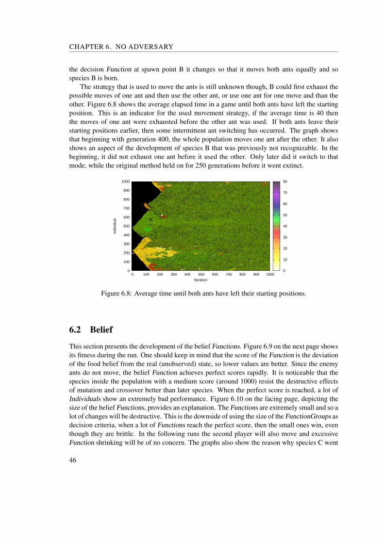
CHAPTER 6. NO ADVERSARY
the decision Function at spawn point B it changes so that it moves both ants equally and sospecies B is born.
The strategy that is used to move the ants is still unknown though, B could first exhaust thepossible moves of one ant and then use the other ant, or use one ant for one move and than theother. Figure 6.8 shows the average elapsed time in a game until both ants have left the startingposition. This is an indicator for the used movement strategy, if the average time is 40 thenthe moves of one ant were exhausted before the other ant was used. If both ants leave theirstarting positions earlier, then some intermittent ant switching has occurred. The graph showsthat beginning with generation 400, the whole population moves one ant after the other. It alsoshows an aspect of the development of species B that was previously not recognizable. In thebeginning, it did not exhaust one ant before it used the other. Only later did it switch to thatmode, while the original method held on for 250 generations before it went extinct.
0
100
200
300
400
500
600
700
800
900
1000
0 100 200 300 400 500 600 700 800 900 1000
Indi
vidu
al
Iteration
0
10
20
30
40
50
60
70
80
Figure 6.8: Average time until both ants have left their starting positions.
6.2 Belief
This section presents the development of the belief Functions. Figure 6.9 on the next page showsits fitness during the run. One should keep in mind that the score of the Function is the deviationof the food belief from the real (unobserved) state, so lower values are better. Since the enemyants do not move, the belief Function achieves perfect scores rapidly. It is noticeable that thespecies inside the population with a medium score (around 1000) resist the destructive effectsof mutation and crossover better than later species. When the perfect score is reached, a lot ofIndividuals show an extremely bad performance. Figure 6.10 on the facing page, depicting thesize of the belief Functions, provides an explanation. The Functions are extremely small and so alot of changes will be destructive. This is the downside of using the size of the FunctionGroups asdecision criteria, when a lot of Functions reach the perfect score, then the small ones win, eventhough they are brittle. In the following runs the second player will also move and excessiveFunction shrinking will be of no concern. The graphs also show the reason why species C went
46

6.3. PREDICTION
0
100
200
300
400
500
600
700
800
900
1000
0 100 200 300 400 500 600 700 800 900 1000
Indi
vidu
al
Iteration
0
1000
2000
3000
4000
5000
Figure 6.9: Development of the deviation of the belief Function.
0
100
200
300
400
500
600
700
800
900
1000
0 100 200 300 400 500 600 700 800 900 1000
Indi
vidu
al
Iteration
0
50
100
150
200
C
Figure 6.10: Size of the belief Functions.
extinct even though it was clearly superior to its neighbours. It depended on its belief Function tobehave in a non-optimal way and when those were replaced by “better” performing ones speciesC could not survive.
6.3 Prediction
The predict Functions did not have anything to do in this run as the opponent ants stayed at theirstarting positions. In the spirit of establishing a base line with which to compare further results,figure 6.11 on the next page shows the development of the score and figure 6.12 on the followingpage the development of the size of the predict Functions. Like the belief Function, the predictFunctions suffer from the problem of brittleness due to a very small size. It is also interesting tonote that a slightly smaller but far more susceptible to destroying changes species took over the
47

CHAPTER 6. NO ADVERSARY
0
100
200
300
400
500
600
700
800
900
1000
0 100 200 300 400 500 600 700 800 900 1000
Indi
vidu
al
Iteration
0
1000
2000
3000
4000
5000
(a) predict 1
0
100
200
300
400
500
600
700
800
900
1000
0 100 200 300 400 500 600 700 800 900 1000
Indi
vidu
al
Iteration
0
1000
2000
3000
4000
5000
(b) predict 2
Figure 6.11: Fitness development of the predict Functions.
0
100
200
300
400
500
600
700
800
900
1000
0 100 200 300 400 500 600 700 800 900 1000
Indi
vidu
al
Iteration
0
20
40
60
80
100
(a) predict 1
0
100
200
300
400
500
600
700
800
900
1000
0 100 200 300 400 500 600 700 800 900 1000
Indi
vidu
al
Iteration
0
20
40
60
80
100
(b) predict 2
Figure 6.12: Size development of the predict Functions.
population. Another effect worth mentioning is that size anomalies (i.e. suddenly bigger than thesurroundings) occur in the populations of the Functions at the same positions due to the allowedcrossover between them.
6.4 General Performance Observations
Figure 6.13 on the next page shows the development of the total population size during the run.As is expected with genetic programming, the size of the population increased steadily from100000 Statements in the beginning to 400000 in the end. Note, however, that the increaseis not monotonic. There are phases where the population is shrinking (in terms of number ofStatements). Figure 6.14 on the facing page shows how the size of the population is distributedamong the Individuals. A correlation between Individual size and fitness can only be observedduring the early generations; the spawn points B and C from figure 6.7 on page 45 can berecognised. After that, size is independent from fitness, i.e. code bloat can be observed. It isinteresting to note that species B barely grows, which is in stark contrast to species A. Due to theexploding population size, one would expect the time needed to evaluate it would also increase.
48
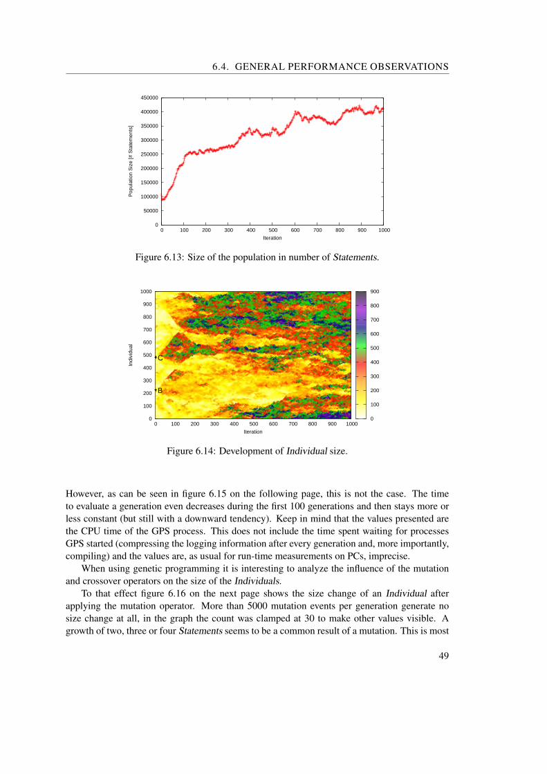
6.4. GENERAL PERFORMANCE OBSERVATIONS
0
50000
100000
150000
200000
250000
300000
350000
400000
450000
0 100 200 300 400 500 600 700 800 900 1000
Pop
ulat
ion
Siz
e [#
Sta
tem
ents
]
Iteration
Figure 6.13: Size of the population in number of Statements.
0
100
200
300
400
500
600
700
800
900
1000
0 100 200 300 400 500 600 700 800 900 1000
Indi
vidu
al
Iteration
0
100
200
300
400
500
600
700
800
900
C
B
Figure 6.14: Development of Individual size.
However, as can be seen in figure 6.15 on the following page, this is not the case. The timeto evaluate a generation even decreases during the first 100 generations and then stays more orless constant (but still with a downward tendency). Keep in mind that the values presented arethe CPU time of the GPS process. This does not include the time spent waiting for processesGPS started (compressing the logging information after every generation and, more importantly,compiling) and the values are, as usual for run-time measurements on PCs, imprecise.
When using genetic programming it is interesting to analyze the influence of the mutationand crossover operators on the size of the Individuals.
To that effect figure 6.16 on the next page shows the size change of an Individual afterapplying the mutation operator. More than 5000 mutation events per generation generate nosize change at all, in the graph the count was clamped at 30 to make other values visible. Agrowth of two, three or four Statements seems to be a common result of a mutation. This is most
49
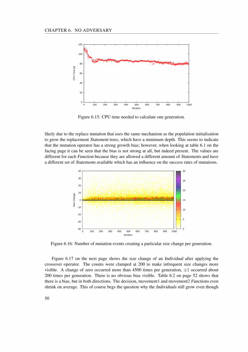
CHAPTER 6. NO ADVERSARY
0
20
40
60
80
100
120
0 100 200 300 400 500 600 700 800 900 1000
CP
U T
ime
[s]
Iteration
Figure 6.15: CPU time needed to calculate one generation.
likely due to the replace mutation that uses the same mechanism as the population initialisationto grow the replacement Statement trees, which have a minimum depth. This seems to indicatethat the mutation operator has a strong growth bias; however, when looking at table 6.1 on thefacing page it can be seen that the bias is not strong at all, but indeed present. The values aredifferent for each Function because they are allowed a different amount of Statements and havea different set of Statements available which has an influence on the success rates of mutations.
-40
-30
-20
-10
0
10
20
30
40
0 100 200 300 400 500 600 700 800 900 1000
Siz
e C
hang
e
Iteration
0
5
10
15
20
25
30
Figure 6.16: Number of mutation events creating a particular size change per generation.
Figure 6.17 on the next page shows the size change of an Individual after applying thecrossover operator. The counts were clamped at 200 to make infrequent size changes morevisible. A change of zero occurred more than 4500 times per generation, ±1 occurred about200 times per generation. There is no obvious bias visible. Table 6.2 on page 52 shows thatthere is a bias, but in both directions. The decision, movement1 and movement2 Functions evenshrink on average. This of course begs the question why the Individuals still grow even though
50

6.5. BEST INDIVIDUALS
Table 6.1: Size change (∆S) of Individuals due to mutation.
Function ∆S σ∆S∆Smin ∆Smax
belief 0.056 1.533 -79 94decision 0.028 3.556 -197 137movement1 0.073 3.913 -283 147movement2 0.070 3.901 -287 162predict1 0.010 0.646 -48 95predict2 0.012 0.721 -21 97
mutation and crossover do not create bigger Functions on average. The answer is that the shrunkIndividuals are less likely to be selected in the next iteration than others because some importantparts of the Statement tree were destroyed and the fitness will suffer. Changes that cause agrowth in size may also destroy important parts but with a smaller probability, so the smallerIndividuals get weeded out by selection and the population grows. From tables 6.1 and 6.2 onthe following page it can be seen that the crossover operator can create more growth than themutation operator, because it can take a big subtree from the donor Function and insert it nearto the leaves in the receiving Function. Mutation has to create new Statement trees, and theirmaximum depth (and so the amount of Statements they can contain) is limited.
-40
-30
-20
-10
0
10
20
30
40
0 100 200 300 400 500 600 700 800 900 1000
Siz
e C
hang
e
Iteration
0
50
100
150
200
Figure 6.17: Number of crossover events creating a particular size change per generation.
6.5 Best Individuals
This section analyzes the properties of the best Individuals per generation. Figure 6.18 on thenext page shows the positions of the best Individual per generation. The spawn points A,B andC from figure 6.7 on page 45 can be easily recognised. There is even an additional spawn point(labeled D in figure 6.18 on the next page) that was not obvious from other figures. The fitness
51
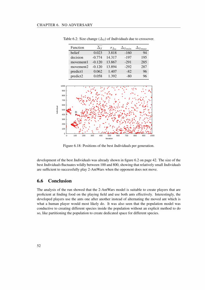
CHAPTER 6. NO ADVERSARY
Table 6.2: Size change (∆S) of Individuals due to crossover.
Function ∆S σ∆S∆Smin ∆Smax
belief 0.023 3.818 -160 94decision -0.774 14.317 -197 195movement1 -0.120 13.867 -291 285movement2 -0.120 13.894 -292 287predict1 0.062 1.407 -82 96predict2 0.058 1.392 -80 96
0
100
200
300
400
500
600
700
800
900
1000
0 100 200 300 400 500 600 700 800 900 1000
Indi
vidu
al
Iteration
D
Figure 6.18: Positions of the best Individuals per generation.
development of the best Individuals was already shown in figure 6.2 on page 42. The size of thebest Individuals fluctuates wildly between 100 and 800, showing that relatively small Individualsare sufficient to successfully play 2-AntWars when the opponent does not move.
6.6 Conclusion
The analysis of the run showed that the 2-AntWars model is suitable to create players that areproficient at finding food on the playing field and use both ants effectively. Interestingly, thedeveloped players use the ants one after another instead of alternating the moved ant which iswhat a human player would most likely do. It was also seen that the population model wasconductive to creating different species inside the population without an explicit method to doso, like partitioning the population to create dedicated space for different species.
52

CHAPTER 7Strategies Version 1
This chapter presents the results of trying to evolve players capable of beating the first implemen-tation of the three discussed strategies in section 3.3 on page 14. During this and the followingchapters, player 1 designates the player that is developed by GPS, player 2 is the player movingaccording to a fixed strategy.
7.1 Greedy
This section presents the results of a run against the Greedy strategy. First the implementationof the strategy is discussed before the run is analyzed in detail.
Implementation
Movement1 and movement2 of the greedy player are the same. During the first four moves, itreturns twice north-west and once north for ant 1 and twice south-east and once south for ant 2 toseparate the ants enough so that they chase different pieces of food. Later, the Function returnsimmediately scoring moves if such moves exist. Otherwise the immediately scoring moves fromthe positions north-east, north-west, south-east and south-west to the current position of the antare compared and the direction with the best scoring potential is returned (if it has at least onescoring move). Then the moves uncovering the most unseen fields are calculated and returned ifthere are moves that uncover unseen fields. In the case that still no moves have been returned,the nearest food position and nearest unseen field position and their distances to the position ofthe ant are calculated. If the distance to the position of the food is not larger than the distanceto the nearest unseen field then the moves towards the food, otherwise the moves towards theunseen field are returned.
The decision Function for the greedy player alternates between moving ant 1 and 2. It alsoprioritizes moves suggested by the movement Functions in the following order: for ant 1 north,south, north-west, south-west; for ant 2 south, north, south-west, north-west. This is done toimprove collection efficiency; before moving away from the starting positions to reach food,
53
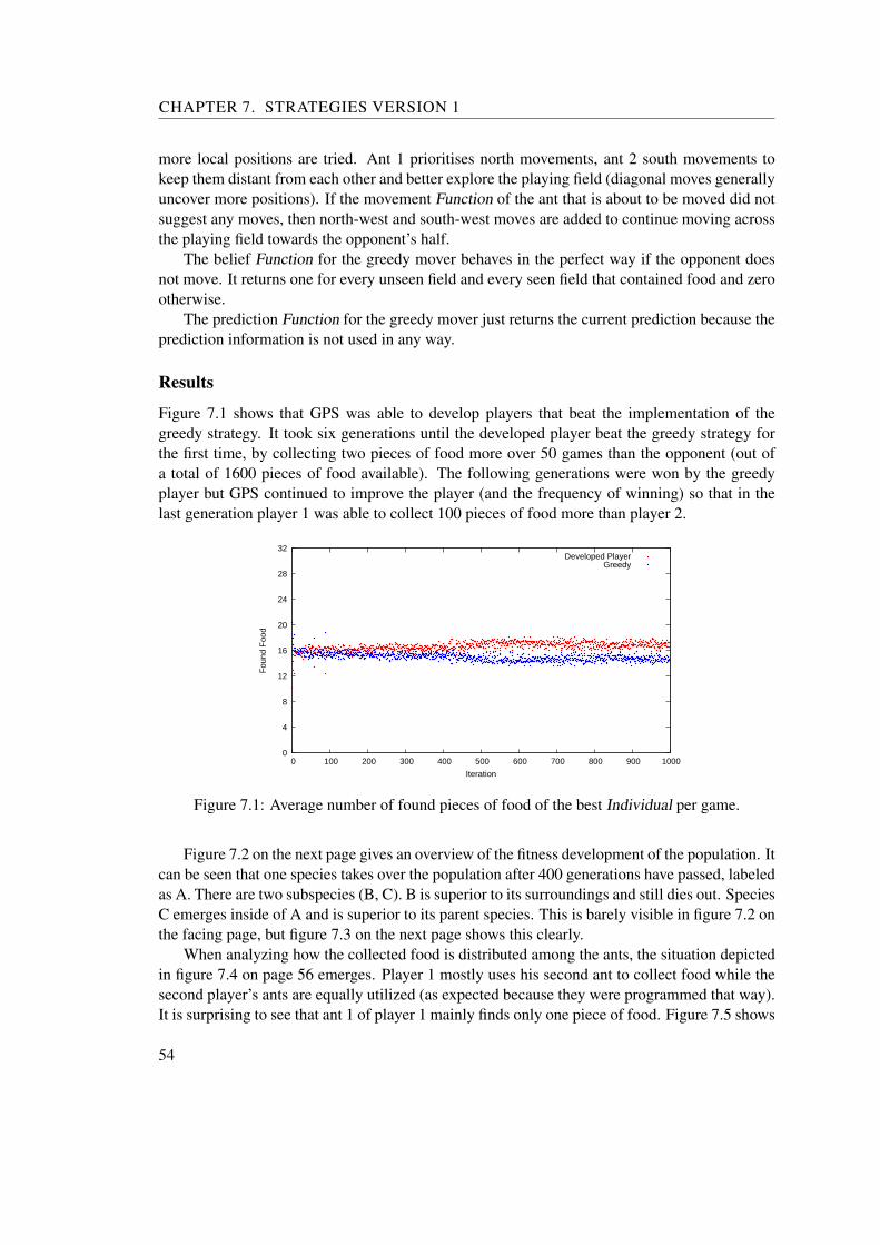
CHAPTER 7. STRATEGIES VERSION 1
more local positions are tried. Ant 1 prioritises north movements, ant 2 south movements tokeep them distant from each other and better explore the playing field (diagonal moves generallyuncover more positions). If the movement Function of the ant that is about to be moved did notsuggest any moves, then north-west and south-west moves are added to continue moving acrossthe playing field towards the opponent’s half.
The belief Function for the greedy mover behaves in the perfect way if the opponent doesnot move. It returns one for every unseen field and every seen field that contained food and zerootherwise.
The prediction Function for the greedy mover just returns the current prediction because theprediction information is not used in any way.
Results
Figure 7.1 shows that GPS was able to develop players that beat the implementation of thegreedy strategy. It took six generations until the developed player beat the greedy strategy forthe first time, by collecting two pieces of food more over 50 games than the opponent (out ofa total of 1600 pieces of food available). The following generations were won by the greedyplayer but GPS continued to improve the player (and the frequency of winning) so that in thelast generation player 1 was able to collect 100 pieces of food more than player 2.
0
4
8
12
16
20
24
28
32
0 100 200 300 400 500 600 700 800 900 1000
Fou
nd F
ood
Iteration
Developed PlayerGreedy
Figure 7.1: Average number of found pieces of food of the best Individual per game.
Figure 7.2 on the next page gives an overview of the fitness development of the population. Itcan be seen that one species takes over the population after 400 generations have passed, labeledas A. There are two subspecies (B, C). B is superior to its surroundings and still dies out. SpeciesC emerges inside of A and is superior to its parent species. This is barely visible in figure 7.2 onthe facing page, but figure 7.3 on the next page shows this clearly.
When analyzing how the collected food is distributed among the ants, the situation depictedin figure 7.4 on page 56 emerges. Player 1 mostly uses his second ant to collect food while thesecond player’s ants are equally utilized (as expected because they were programmed that way).It is surprising to see that ant 1 of player 1 mainly finds only one piece of food. Figure 7.5 shows
54

7.1. GREEDY
0
100
200
300
400
500
600
700
800
900
1000
0 100 200 300 400 500 600 700 800 900 1000
Indi
vidu
al
Iteration
0
20
40
60
80
100
120
A
B
C
Figure 7.2: Found food of the Individuals playing 2-AntWars against a Greedy player.
0
100
200
300
400
500
600
700
800
900
1000
0 100 200 300 400 500 600 700 800 900 1000
Indi
vidu
al
Iteration
Figure 7.3: Location of the best Individual inside the population of a particular generation.
that Player 1 uses one ant until it cannot move anymore before the other one is moved. Combinedwith the fact that ant 2 collects more food than ant 1 this means that player 1 uses ant 2 first andthen ant 1. Not every Individual of the population uses this method though, figure 7.5 on thenext page shows at least one distinct subspecies (labeled D) that moves both ants earlier.
It was shown before that there is a species inside the population that is superior to its neigh-bors but still dies out (species B, figure 7.2). Figure 7.6 on page 57 shows the reason: The beliefFunction that B uses gets replaced by a slightly better (but a lot brittler) Function. Now thatplayer 2 actually moves, the population does not converge to extremely small and extremelybrittle Functions as seen in the run without adversary, but still the better belief Functions seemto be more susceptible to catastrophic change.
Figure 7.7 on page 57 shows the fitness of the belief Function that was used by the bestIndividual in each generation. Three distinct levels of fitness can be observed, the first corre-
55

CHAPTER 7. STRATEGIES VERSION 1
0
5
10
15
20
25
0 100 200 300 400 500 600 700 800 900 1000
Fou
nd F
ood
Iteration
0
50
100
150
200
(a) Player 1 Ant 1
0
5
10
15
20
25
0 100 200 300 400 500 600 700 800 900 1000
Fou
nd F
ood
Iteration
0
50
100
150
200
(b) Player 1 Ant 2
0
5
10
15
20
25
0 100 200 300 400 500 600 700 800 900 1000
Fou
nd F
ood
Iteration
0
50
100
150
200
(c) Player 2 Ant 1
0
5
10
15
20
25
0 100 200 300 400 500 600 700 800 900 1000
Fou
nd F
ood
Iteration
0
50
100
150
200
(d) Player 2 Ant 2
Figure 7.4: Distribution of found food per ant.
0
100
200
300
400
500
600
700
800
900
1000
0 100 200 300 400 500 600 700 800 900 1000
Indi
vidu
al
Iteration
0
10
20
30
40
50
60
70
80
D
Figure 7.5: Average time when both ants of the developed player leave the starting position.
56

7.1. GREEDY
0
100
200
300
400
500
600
700
800
900
1000
0 100 200 300 400 500 600 700 800 900 1000
Indi
vidu
al
Iteration
0
1000
2000
3000
4000
5000
B
Figure 7.6: Development of the belief deviation.
0
200
400
600
800
1000
0 100 200 300 400 500 600 700 800 900 1000
Bel
ief D
evia
tion
Iteration
Developed PlayerGreedy
Figure 7.7: Average belief deviation of the best Individual per game.
sponding to species A, the second to species B and the third to species C. Only the third level isbetter than the belief Function of player 2, which shows that it is hard for GPS to find a suitablebelief Function. The belief Function in the last generation has an average deviation of 343.4 pergame. It reaches that deviation by beginning with a belief of one at every unseen position andslowly reducing it until it reaches about−0.07 when the game ends (the actual value depends onthe length of the game). The belief depends on the time that has passed but not on the predictedpositions of the enemy’s ants (or any position at all). The belief in food that was seen but iscurrently not visible is 0.8.
The fitness of the other auxiliary Functions (predict1 and predict2) of the best Individualper generation is shown in figure 7.8 on the next page. It can be seen that the performance ofplayer 1’s predict Functions is relatively stable compared to player 2’s Functions. Player 2 isvery bad at predicting the position of ant 2 of player 1 because as determined earlier, this ant is
57

CHAPTER 7. STRATEGIES VERSION 1
0
500
1000
1500
2000
2500
3000
3500
4000
0 100 200 300 400 500 600 700 800 900 1000
Pre
dict
Dev
iatio
n
Iteration
Developed Player predict0Developed Player predict1
Greedy predict0Greedy predict1
Figure 7.8: Average predict deviation of the best Individual and its opponent per game.
0
100
200
300
400
500
600
700
800
900
1000
0 100 200 300 400 500 600 700 800 900 1000
Indi
vidu
al
Iteration
0
1
2
3
4
5
Figure 7.9: Average food remaining on the playing field after a game.
moved first so that predicting it at the starting position is wrong during the whole game. Theprediction of ant 1 of player 2 is not so bad and comparable to the performance of the predictionFunctions of player 1. It is, however, less stable. Player 1 reaches his prediction performance bymoving the predicted positions one field to the west of the current prediction every third moveto approximate the positions of the enemy’s ants.
The average food remaining on the playing field after a game is presented in figure 7.9.It starts with a maximum of 12, but as the Individuals in the population increase their fitness,less and less food remains on the playing field so that in the last generation only 0.52 pieces offood remain uneaten per game. This shows that when two players are active nearly all pieces offood can be collected without needing a suitable positioning bias as was the case when only oneplayer was moving.
58

7.1. GREEDY
The total size of the population and the time needed to evaluate it are depicted in figure 7.10.As was already seen in the run without adversary, the time needed to evaluate a populationis not influenced by its size in Statements. The fitness of the players is more influential asfitter players find all of the available food faster which shortens the games and reduces thecomputational burden. From generation 300 onward, the size of the best Individual is above300. This indicates that playing successfully against moving opponents requires more complexprograms than playing against stationary opponents.
0
100000
200000
300000
400000
500000
600000
700000
0 100 200 300 400 500 600 700 800 900 1000
Pop
ulat
ion
Siz
e [#
Sta
tem
ents
]
Iteration
(a)
0
20
40
60
80
100
120
140
0 100 200 300 400 500 600 700 800 900 1000
CP
U T
ime
[s]
Iteration
(b)
Figure 7.10: (a) Total number of Statements contained in the population and (b) the time neededto evaluate them.
59

CHAPTER 7. STRATEGIES VERSION 1
7.2 Scorched Earth
This section discusses the run against the Scorched Earth strategy. As before, the implementationwill be presented before the result is analyzed.
Implementation
The decision Function lets every ant move once before the other ant is moved.The movement Functions move the ants in the following way: When the game begins, move-
ment1 moves the ant to position (9, 2), movement2 to position (9, 10), which brings them oneposition into the playing field half of player 1. Food is ignored on the way. Then the ants aremoved north and south until all food on positions with the same y-coordinate as theirs is eatenor all positions have been seen. After that, the ants are moved west once and the process isrepeated. Figure 7.11 shows the movement path of the ants with this implementation of theScorched Earth strategy.
The belief and predict Functions are the same as the ones the Greedy strategy used, i.e. beliefas if the other player did not exist and predict always the last prediction.
Figure 7.11: Player 2 using the first implementation of the Scorched Earth strategy.
60

7.2. SCORCHED EARTH
0
4
8
12
16
20
24
28
32
0 100 200 300 400 500 600 700 800 900 1000
Fou
nd F
ood
Iteration
Developed PlayerScorched Earth
Figure 7.12: Average number of found pieces of food of the best Individual per game.
0
200
400
600
800
1000
0 100 200 300 400 500 600 700 800 900 1000
Bel
ief D
evia
tion
Iteration
Developed PlayerScorched Earth
Figure 7.13: Average belief deviation of the best Individual and its opponent per game.
Results
Figure 7.12 shows that GPS had no problem developing players that are capable of beatingthe first implementation of the Scorched Earth strategy. Beginning with the second generation,the best Individual always performed better than its opponent (with the exception of generation9). During the first 100 generations, the fitness of the Individuals improves steadily, then itstagnates for 100 generations before it suddenly jumps to its final value. The reason for this lastimprovement was found by watching the games of the best Individuals of generation 150 and200. In both games the players exploited the rigidity of the Scorched Earth player and sent oneant into his half while his ants were still moving towards the center of the playing field. Therethey collected some food, ensuring that the Scorched Earth player cannot win. One might saythat Scorched Earth was beaten by a more efficient form of Scorched Earth. The innovation of
61

CHAPTER 7. STRATEGIES VERSION 1
0
500
1000
1500
2000
2500
3000
3500
4000
0 100 200 300 400 500 600 700 800 900 1000
Pre
dict
Dev
iatio
n
Iteration
Developed Player predict0Developed Player predict1
Scorched Earth predict0Scorched Earth predict1
Figure 7.14: Average predict deviation of the best Individual and its opponent per game.
0
100
200
300
400
500
600
700
800
900
1000
0 100 200 300 400 500 600 700 800 900 1000
Indi
vidu
al
Iteration
0
20
40
60
80
100
120
140
A B1
B2
B3
B
Figure 7.15: Found food of the Individuals playing 2-AntWars against a Scorched Earth player.
the player at generation 200 was that the ants did not always act greedily while moving towardsthe half of player 2. There were situations where the ant could have moved one field backwardsto eat one piece of food but did not do it. Instead, the ant moved towards the enemy’s half of theplaying field (not ignoring the food on the way), was there earlier than the player of generation150 and collected more food there.
The average belief deviation of the best Individual per generation depicted in figure 7.13on the preceding page shows the same development as the amount of eaten food. First it im-proves steadily and then it stagnates before jumping to its final value. The average deviation ofthe Scorched Earth player is significantly higher than the deviation of the Greedy player (seefigure 7.7 on page 57), even though they use the same Function. The reason for that is that theScorched Earth player believes that the food he passes on his way to the center of the playingfield stays there, but in reality it is eaten by the developed player .
62

7.2. SCORCHED EARTH
0
100
200
300
400
500
600
700
800
900
1000
0 100 200 300 400 500 600 700 800 900 1000
Indi
vidu
al
Iteration
0
20
40
60
80
100
120
A B1
B2
B3
B
C1 C2
D
(a) Ant 1
0
100
200
300
400
500
600
700
800
900
1000
0 100 200 300 400 500 600 700 800 900 1000
Indi
vidu
al
Iteration
0
20
40
60
80
100
120
A B1
B2
B3
B
C1 C2
D
(b) Ant 2
Figure 7.16: Found food of the ants of player 1 against the Scorched Earth strategy.
0
100
200
300
400
500
600
700
800
900
1000
0 100 200 300 400 500 600 700 800 900 1000
Indi
vidu
al
Iteration
0
0.2
0.4
0.6
0.8
1
(a) Ant 1
0
100
200
300
400
500
600
700
800
900
1000
0 100 200 300 400 500 600 700 800 900 1000
Indi
vidu
al
Iteration
0
0.2
0.4
0.6
0.8
1
(b) Ant 2
Figure 7.17: Probability that an ant of player 1 is still movable after the game has ended.
Figure 7.14 on the facing page shows that the predict Functions reached the same level ofprecision as in the run against the Greedy player, but the method by which it was reached wasdifferent. The predict1 Function constantly returned (14, 3) as prediction, predict2 returned(14, 9). Instead of moving the prediction around, it was placed at the center of the path the antsmove on.
The overview of the fitness development of the run against the Scorched Earth player is givenin figure 7.15 on the preceding page. After 100 generations, species A formed and took over thepopulation. At spawn points B1, B2 and B3 improvements to A emerged that formed speciesB which was the only species present in the population by generation 450. Figure 7.16 gives amore detailed insight into the development of the population by separating the performances ofant 1 and ant 2 of player 1. It shows that from this point of view, species A is not a coherentspecies at all but rather a conglomerate of at least three species. The change to species B wasmostly achieved by improving the performance of ant 1 while the one of ant 2 stays the same.Species B is also not as homogenous as it seemed. The predominant behaviour is that ant 2moves first until it has no moves left and then ant 1 starts to move (see also figure 7.17) butthere are two species hidden inside it (C2 and D) that have switched the role of ant 1 and ant 2.
63
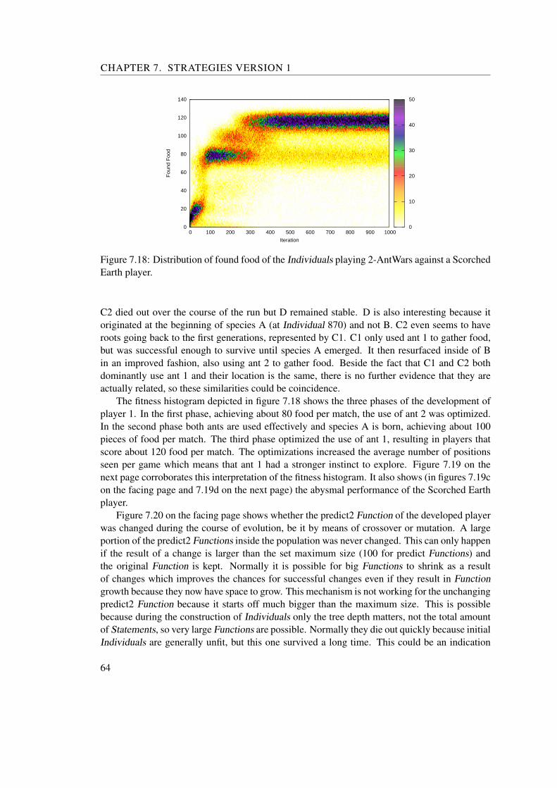
CHAPTER 7. STRATEGIES VERSION 1
0
20
40
60
80
100
120
140
0 100 200 300 400 500 600 700 800 900 1000
Fou
nd F
ood
Iteration
0
10
20
30
40
50
Figure 7.18: Distribution of found food of the Individuals playing 2-AntWars against a ScorchedEarth player.
C2 died out over the course of the run but D remained stable. D is also interesting because itoriginated at the beginning of species A (at Individual 870) and not B. C2 even seems to haveroots going back to the first generations, represented by C1. C1 only used ant 1 to gather food,but was successful enough to survive until species A emerged. It then resurfaced inside of Bin an improved fashion, also using ant 2 to gather food. Beside the fact that C1 and C2 bothdominantly use ant 1 and their location is the same, there is no further evidence that they areactually related, so these similarities could be coincidence.
The fitness histogram depicted in figure 7.18 shows the three phases of the development ofplayer 1. In the first phase, achieving about 80 food per match, the use of ant 2 was optimized.In the second phase both ants are used effectively and species A is born, achieving about 100pieces of food per match. The third phase optimized the use of ant 1, resulting in players thatscore about 120 food per match. The optimizations increased the average number of positionsseen per game which means that ant 1 had a stronger instinct to explore. Figure 7.19 on thenext page corroborates this interpretation of the fitness histogram. It also shows (in figures 7.19con the facing page and 7.19d on the next page) the abysmal performance of the Scorched Earthplayer.
Figure 7.20 on the facing page shows whether the predict2 Function of the developed playerwas changed during the course of evolution, be it by means of crossover or mutation. A largeportion of the predict2 Functions inside the population was never changed. This can only happenif the result of a change is larger than the set maximum size (100 for predict Functions) andthe original Function is kept. Normally it is possible for big Functions to shrink as a resultof changes which improves the chances for successful changes even if they result in Functiongrowth because they now have space to grow. This mechanism is not working for the unchangingpredict2 Function because it starts off much bigger than the maximum size. This is possiblebecause during the construction of Individuals only the tree depth matters, not the total amountof Statements, so very large Functions are possible. Normally they die out quickly because initialIndividuals are generally unfit, but this one survived a long time. This could be an indication
64
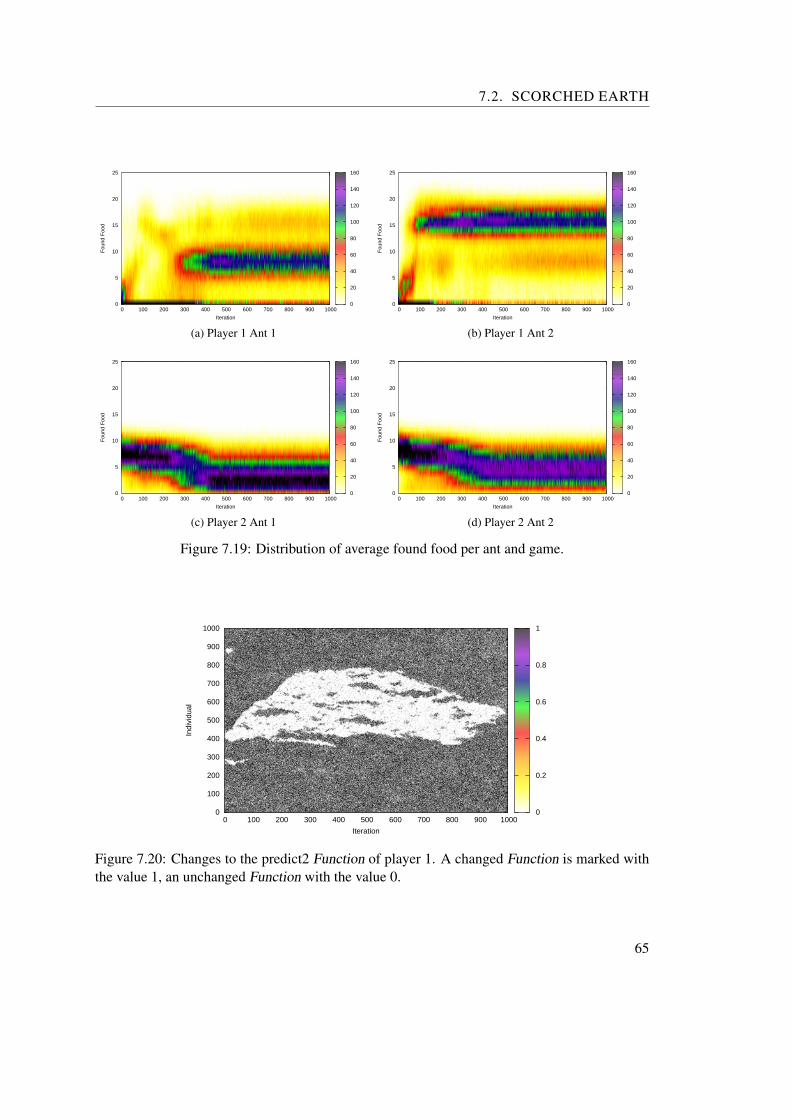
7.2. SCORCHED EARTH
0
5
10
15
20
25
0 100 200 300 400 500 600 700 800 900 1000
Fou
nd F
ood
Iteration
0
20
40
60
80
100
120
140
160
(a) Player 1 Ant 1
0
5
10
15
20
25
0 100 200 300 400 500 600 700 800 900 1000
Fou
nd F
ood
Iteration
0
20
40
60
80
100
120
140
160
(b) Player 1 Ant 2
0
5
10
15
20
25
0 100 200 300 400 500 600 700 800 900 1000
Fou
nd F
ood
Iteration
0
20
40
60
80
100
120
140
160
(c) Player 2 Ant 1
0
5
10
15
20
25
0 100 200 300 400 500 600 700 800 900 1000
Fou
nd F
ood
Iteration
0
20
40
60
80
100
120
140
160
(d) Player 2 Ant 2
Figure 7.19: Distribution of average found food per ant and game.
0
100
200
300
400
500
600
700
800
900
1000
0 100 200 300 400 500 600 700 800 900 1000
Indi
vidu
al
Iteration
0
0.2
0.4
0.6
0.8
1
Figure 7.20: Changes to the predict2 Function of player 1. A changed Function is marked withthe value 1, an unchanged Function with the value 0.
65

CHAPTER 7. STRATEGIES VERSION 1
0
100
200
300
400
500
600
700
800
900
1000
0 100 200 300 400 500 600 700 800 900 1000
Indi
vidu
al
Iteration
0
10
20
30
40
50
60
70
80
E
F
(a) First time both moved
0
100
200
300
400
500
600
700
800
900
1000
0 100 200 300 400 500 600 700 800 900 1000
Indi
vidu
al
Iteration
0
0.2
0.4
0.6
0.8
1
(b) Both collecting food
Figure 7.21: Effective use of both ants.
0
100000
200000
300000
400000
500000
600000
700000
0 100 200 300 400 500 600 700 800 900 1000
Pop
ulat
ion
Siz
e [#
Sta
tem
ents
]
Iteration
(a)
0
20
40
60
80
100
120
0 100 200 300 400 500 600 700 800 900 1000
CP
U T
ime
[s]
Iteration
(b)
Figure 7.22: (a) Total number of Statements contained in the population and (b) the time neededto evaluate them.
that the size limit of 100 is too small because a static large Function survived a long time againstevolving and improving smaller Functions.
The effective use of both ants is analyzed in figure 7.21. Figure 7.21a shows the average ofthe first time per game when both ants have left their starting positions. The use of both ants waspresent in the population from the beginning, but only effective when species A emerged. Thereare also two additional species visible (E,F) that move both ants earlier. Note that F is a partof D. The population also contains some very small species that move both ants nearly at thebeginning of the game. As figure 7.21b indicates, those small species use both ants effectivelyand are not simply defective Individuals. This is the behaviour one would expect from a humanplayer (moving both ants “simultaneously” and collecting food with both), so GPS is indeedable to develop it; however, it does not survive against the more common strategy of moving oneant until the moves run out and then the other.
As always, the end of the discussion of a run is a look at the development of the size of thepopulation and the time needed to evaluate it, provided by figure 7.22. The size of the populationrises fast towards 600000 Statements, which is the same value that was seen in the discussionof the Greedy strategy. Again, the time needed to evaluate the population is independent of theactual size (in Statements) of the population.
66

7.3. HUNTER
7.3 Hunter
This section discusses the run against the Hunter strategy.
Implementation
The Hunter implementation assigns two roles to its ants. Ant 1 is the hunter and therefore doingall the hunting, and Ant 2 is the gatherer, doing no hunting but tasked with collecting as muchfood as possible to make the implementation more productive. Movement1 does not return anymoves because the move for the hunter ant is calculated by the decision Function, which hasaccess to the position predictions of the enemy’s ants. Movement2 uses the movement Functionof the Greedy strategy, see section 7.1 on page 53 for its implementation. The decision Functiondecides to use the hunter ant as long as it is movable and the gatherer ant otherwise. If the hunterant is chosen, its move is calculated in the following way: If the hunter ant is one move awayfrom one of the ants, it attacks immediately. Otherwise the moves towards the enemy’s ants(predicted) positions (if they were seen movable) and towards food that is reachable with onemove are calculated. The intersections of the following moves are tried in that order and returnedif they are not empty: all three moves, move towards nearer ant and food, move towards nearerant. If this does not result in any move (for example if both ants were already neutralized) themovement Function of the Greedy strategy is used to determine the move of the hunting ant. Thebelief Function uses the same method to calculate the food belief as the Greedy and ScorchedEarth implementations. The implementation of the predict Functions was a bit tricky, becauseit is not really possible to predict how the enemy’s ants move before the run, so the predictionwas simply moved randomly either one position north-east, east or south-east from the currentprediction every second move. If the predicted position is visible and the enemy’s ant is not onit then the nearest unseen position to the predicted position is chosen as new prediction.
Results
Figure 7.23 on the following page shows that GPS was able to evolve players that beat the Hunterstrategy, but it took 700 generations to do so. Interestingly, the developed belief Function wasnot able to beat the belief Function of the Hunter (figure 7.24a on the next page), unlike the twoprevious runs. The next figure (7.24b on the following page) shows that the predict Functionsfor the Hunter are not better than the “do not predict” Functions of the Greedy and ScorchedEarth strategies and that the developed player uses prediction Functions that beat them in termsof precision. Also note that the prediction accuracy of predict1 is better than for predict2, whichis no surprise because the hunting ant behaves more predictably than the gathering ant. It is alsohelpful that the hunting ant tries to be close to player 1’s ants so that it is seen and thereforeaccurately predicted. The study of the games of the best Individuals showed that predict 1 of thedeveloped player is very close to the actual position of the hunter ant on its way to the startingposition of player 1.
The fitness development of the whole population (figure 7.25 on page 69) shows speciesA spread throughout the population to be replaced by the successors B and C. As figure 7.26on page 69 shows, A spreads because it uses both of its ants to gather food. However, this
67
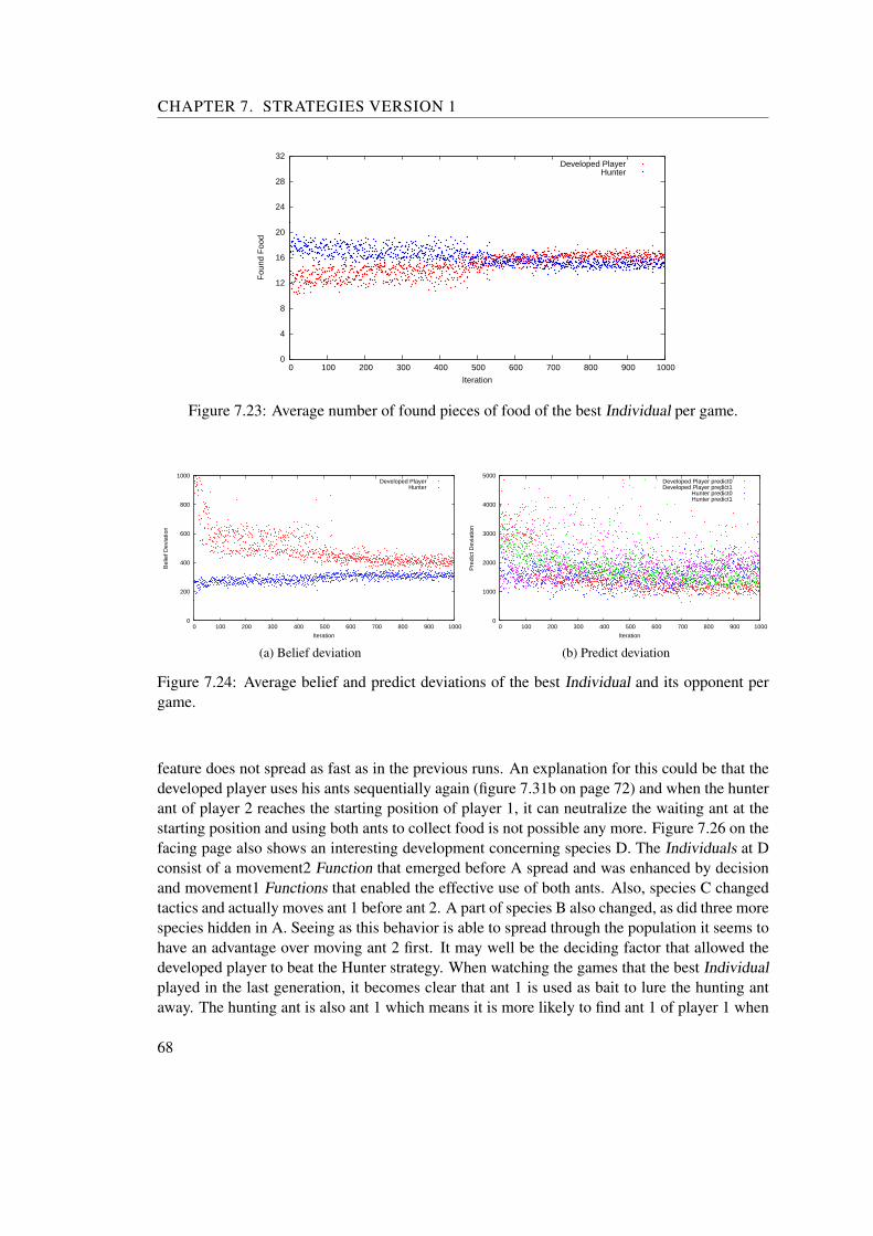
CHAPTER 7. STRATEGIES VERSION 1
0
4
8
12
16
20
24
28
32
0 100 200 300 400 500 600 700 800 900 1000
Fou
nd F
ood
Iteration
Developed PlayerHunter
Figure 7.23: Average number of found pieces of food of the best Individual per game.
0
200
400
600
800
1000
0 100 200 300 400 500 600 700 800 900 1000
Bel
ief D
evia
tion
Iteration
Developed PlayerHunter
(a) Belief deviation
0
1000
2000
3000
4000
5000
0 100 200 300 400 500 600 700 800 900 1000
Pre
dict
Dev
iatio
n
Iteration
Developed Player predict0Developed Player predict1
Hunter predict0Hunter predict1
(b) Predict deviation
Figure 7.24: Average belief and predict deviations of the best Individual and its opponent pergame.
feature does not spread as fast as in the previous runs. An explanation for this could be that thedeveloped player uses his ants sequentially again (figure 7.31b on page 72) and when the hunterant of player 2 reaches the starting position of player 1, it can neutralize the waiting ant at thestarting position and using both ants to collect food is not possible any more. Figure 7.26 on thefacing page also shows an interesting development concerning species D. The Individuals at Dconsist of a movement2 Function that emerged before A spread and was enhanced by decisionand movement1 Functions that enabled the effective use of both ants. Also, species C changedtactics and actually moves ant 1 before ant 2. A part of species B also changed, as did three morespecies hidden in A. Seeing as this behavior is able to spread through the population it seems tohave an advantage over moving ant 2 first. It may well be the deciding factor that allowed thedeveloped player to beat the Hunter strategy. When watching the games that the best Individualplayed in the last generation, it becomes clear that ant 1 is used as bait to lure the hunting antaway. The hunting ant is also ant 1 which means it is more likely to find ant 1 of player 1 when
68

7.3. HUNTER
moving across the playing field. It then follows ant 1 (the lure) which is busy collecting foodand moving away from the starting position (and from ant 2). When the hunter finally catchesup with the bait, it has already eaten some food and is quite a distance away from ant 2, so ant 2can begin to collect food unhindered. Furthermore, the hunter already spent a lot of moves onhunting and will not reach ant 2 in time. The gatherer ant does not hunt the remaining ant ofplayer 1, so player 1 is able to win.
0
100
200
300
400
500
600
700
800
900
1000
0 100 200 300 400 500 600 700 800 900 1000
Indi
vidu
al
Iteration
0
20
40
60
80
100
120
A
B
C
Figure 7.25: Found food of the Individuals playing 2-AntWars against a Hunter player.
0
100
200
300
400
500
600
700
800
900
1000
0 100 200 300 400 500 600 700 800 900 1000
Indi
vidu
al
Iteration
0
20
40
60
80
100
120D
C
(a) Ant 1
0
100
200
300
400
500
600
700
800
900
1000
0 100 200 300 400 500 600 700 800 900 1000
Indi
vidu
al
Iteration
0
20
40
60
80
100
120D
C
(b) Ant 2
Figure 7.26: Found food of the ants of player 1 against the Hunter strategy.
The histogram of the fitness development (figure 7.27 on the next page) shows that thepopulation as a whole fails to reach the 80 pieces of food mark and that it is not as clearly splitup into different performance levels as the populations in the previous runs were. The reasonfor this is seen in figure 7.28 on the following page. The performance of both ants of player 1is distributed among the same two levels which are the result of choosing one ant or the otherto move first. Unsurprisingly, the performance of ant 2 of player 2 is better than that of ant 1because it is the gatherer ant’s job to be good at collecting food.
69

CHAPTER 7. STRATEGIES VERSION 1
0
20
40
60
80
100
120
140
0 100 200 300 400 500 600 700 800 900 1000
Fou
nd F
ood
Iteration
0
5
10
15
20
25
30
35
40
Figure 7.27: Distribution of found food of the Individuals playing 2-AntWars against a Hunterplayer.
0
5
10
15
20
25
0 100 200 300 400 500 600 700 800 900 1000
Fou
nd F
ood
Iteration
0
20
40
60
80
100
120
(a) Player 1 Ant 1
0
5
10
15
20
25
0 100 200 300 400 500 600 700 800 900 1000
Fou
nd F
ood
Iteration
0
20
40
60
80
100
120
(b) Player 1 Ant 2
0
5
10
15
20
25
0 100 200 300 400 500 600 700 800 900 1000
Fou
nd F
ood
Iteration
0
20
40
60
80
100
120
(c) Player 2 Ant 1
0
5
10
15
20
25
0 100 200 300 400 500 600 700 800 900 1000
Fou
nd F
ood
Iteration
0
20
40
60
80
100
120
(d) Player 2 Ant 2
Figure 7.28: Distribution of average found food per ant and game.
70

7.3. HUNTER
0
100
200
300
400
500
600
700
800
900
1000
0 100 200 300 400 500 600 700 800 900 1000
Indi
vidu
al
Iteration
0
0.2
0.4
0.6
0.8
1
Figure 7.29: The developed ants winning against the Hunter strategy.
0
100
200
300
400
500
600
700
800
900
1000
0 100 200 300 400 500 600 700 800 900 1000
Indi
vidu
al
Iteration
0
0.5
1
1.5
2
(a) Player 1
0
100
200
300
400
500
600
700
800
900
1000
0 100 200 300 400 500 600 700 800 900 1000
Indi
vidu
al
Iteration
0
0.5
1
1.5
2
(b) Player 2
Figure 7.30: Number of times a player supported a battle with his second ant during a match.
Figure 7.29 gives an interesting view on the result of the matches played by the population.Even though it took 700 generations for the best Individual to start consistently beating thehunter strategy, single matches were won much earlier.
The most surprising result of this run is shown in figure 7.30a. There are actually multiplespecies contained in A that use the battle support rule to win fights against player 2. It does nothappen often (once of a maximum of ten during a match), but it does happen and it is not onlycoincidence, because figure 7.30b shows how often player 2 supported his battles even thoughhe was not programmed to do so; it rarely happened.
Figures 7.31a on the following page and 7.31b on the next page show that the population isstill very diverse from generations 700 to 1000 regarding the movement probabilities of the antsand when both ants are used for the first time. Figure 7.31b on the following page indicates thatmoving both ants earlier than after 40 moves is spreading inside the population. This could bean effect of the lure strategy, where the luring ant does not use its full 40 moves before it getscaught.
71

CHAPTER 7. STRATEGIES VERSION 1
0
100
200
300
400
500
600
700
800
900
1000
0 100 200 300 400 500 600 700 800 900 1000
Indi
vidu
al
Iteration
0
0.2
0.4
0.6
0.8
1
(a) Probability of choosing ant 1 for movement
0
100
200
300
400
500
600
700
800
900
1000
0 100 200 300 400 500 600 700 800 900 1000
Indi
vidu
al
Iteration
0
10
20
30
40
50
60
70
80
(b) Average time until both ants leave their starting posi-tions
Figure 7.31: Indicators of the decision method used by player 1 against the Hunter strategy.
0
100000
200000
300000
400000
500000
600000
700000
0 100 200 300 400 500 600 700 800 900 1000
Pop
ulat
ion
Siz
e [#
Sta
tem
ents
]
Iteration
(a)
0
20
40
60
80
100
120
140
0 100 200 300 400 500 600 700 800 900 1000
CP
U T
ime
[s]
Iteration
(b)
Figure 7.32: (a) Total number of Statements contained in the population and (b) the time neededto evaluate them.
The size development of the population (figure 7.32a) and the time needed to evaluate ongeneration (figure 7.32b) offer no surprises. The total number of Statements contained in thepopulation rises fast towards 600000 but does not effect the execution time. The execution timeis on a higher level than in the run against the Scorched Earth strategy, at least partly becausethe Hunter strategy is computationally more expensive.
72

CHAPTER 8Strategies Version 2
For this chapter, the implementation of the strategies from the previous chapter was improved.Section 8.1 contains the documentation of the run against the second implementation of theGreedy strategy, section 8.2 on page 79 presents the improved Scorched Earth strategy andsection 8.3 on page 84 the Hunter strategy.
8.1 Greedy
Implementation
The movement Function (used for both movement1 and movement2) of the second implementa-tion of the Greedy strategy was, compared to the first implementation, greatly simplified. It onlyuses the functionality provided by the NearestFood Statement. When it is executed, it calcu-lates the Moves towards the nearest, second nearest and third nearest food positions and returnsthe intersection of those Moves if it is not empty, or the intersection of the nearest and secondnearest (if not empty) or just the Moves towards the nearest food positions.
The decision Function was modelled after the results of the runs against the first imple-mentations. In all cases, the developed players used the ants sequentially which seemed to beadvantageous, so the decision Function uses ant 1 as long as it is movable and ant 2 otherwise.
The predict Functions are still of no concern to the Greedy strategy and simply return theprevious prediction.
The belief Function behaves as it did in the original implementations, i.e. believe that food ison positions that were not previously seen and that food seen previously stays there (and is noteaten by enemy ants). The belief in food at unseen positions is also necessary to keep exploringthe playing field, because otherwise the movement Functions would not return Moves if the antshave not seen food, as the implementation of the NearestFood Statement is based on food belief.
73
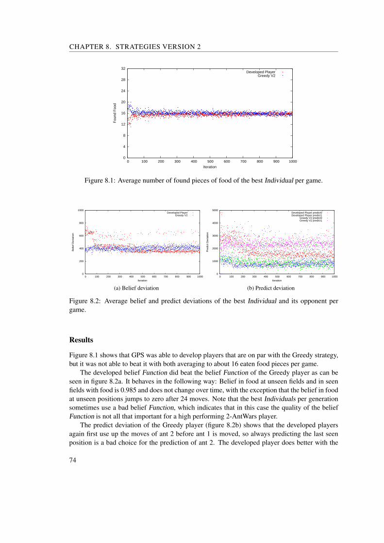
CHAPTER 8. STRATEGIES VERSION 2
0
4
8
12
16
20
24
28
32
0 100 200 300 400 500 600 700 800 900 1000
Fou
nd F
ood
Iteration
Developed PlayerGreedy V2
Figure 8.1: Average number of found pieces of food of the best Individual per game.
0
200
400
600
800
1000
0 100 200 300 400 500 600 700 800 900 1000
Bel
ief D
evia
tion
Iteration
Developed PlayerGreedy V2
(a) Belief deviation
0
1000
2000
3000
4000
5000
0 100 200 300 400 500 600 700 800 900 1000
Pre
dict
Dev
iatio
n
Iteration
Developed Player predict0Developed Player predict1
Greedy V2 predict0Greedy V2 predict1
(b) Predict deviation
Figure 8.2: Average belief and predict deviations of the best Individual and its opponent pergame.
Results
Figure 8.1 shows that GPS was able to develop players that are on par with the Greedy strategy,but it was not able to beat it with both averaging to about 16 eaten food pieces per game.
The developed belief Function did beat the belief Function of the Greedy player as can beseen in figure 8.2a. It behaves in the following way: Belief in food at unseen fields and in seenfields with food is 0.985 and does not change over time, with the exception that the belief in foodat unseen positions jumps to zero after 24 moves. Note that the best Individuals per generationsometimes use a bad belief Function, which indicates that in this case the quality of the beliefFunction is not all that important for a high performing 2-AntWars player.
The predict deviation of the Greedy player (figure 8.2b) shows that the developed playersagain first use up the moves of ant 2 before ant 1 is moved, so always predicting the last seenposition is a bad choice for the prediction of ant 2. The developed player does better with the
74
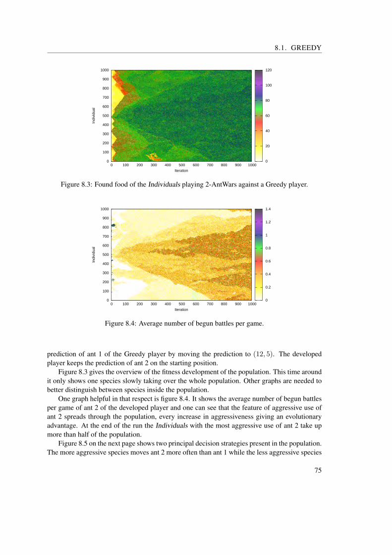
8.1. GREEDY
0
100
200
300
400
500
600
700
800
900
1000
0 100 200 300 400 500 600 700 800 900 1000
Indi
vidu
al
Iteration
0
20
40
60
80
100
120
Figure 8.3: Found food of the Individuals playing 2-AntWars against a Greedy player.
0
100
200
300
400
500
600
700
800
900
1000
0 100 200 300 400 500 600 700 800 900 1000
Indi
vidu
al
Iteration
0
0.2
0.4
0.6
0.8
1
1.2
1.4
Figure 8.4: Average number of begun battles per game.
prediction of ant 1 of the Greedy player by moving the prediction to (12, 5). The developedplayer keeps the prediction of ant 2 on the starting position.
Figure 8.3 gives the overview of the fitness development of the population. This time aroundit only shows one species slowly taking over the whole population. Other graphs are needed tobetter distinguish between species inside the population.
One graph helpful in that respect is figure 8.4. It shows the average number of begun battlesper game of ant 2 of the developed player and one can see that the feature of aggressive use ofant 2 spreads through the population, every increase in aggressiveness giving an evolutionaryadvantage. At the end of the run the Individuals with the most aggressive use of ant 2 take upmore than half of the population.
Figure 8.5 on the next page shows two principal decision strategies present in the population.The more aggressive species moves ant 2 more often than ant 1 while the less aggressive species
75

CHAPTER 8. STRATEGIES VERSION 2
0
100
200
300
400
500
600
700
800
900
1000
0 100 200 300 400 500 600 700 800 900 1000
Indi
vidu
al
Iteration
0
0.2
0.4
0.6
0.8
1
Figure 8.5: Probability that player 1 choosesant 1 for movement.
0
100
200
300
400
500
600
700
800
900
1000
0 100 200 300 400 500 600 700 800 900 1000
Indi
vidu
al
Iteration
0
1
Figure 8.6: Player 2 not finding food withboth ants.
uses the ants with equal probability. Furthermore, the usage of both ants originated from fourplayers in the original population, where one died out, two merged into the less aggressivespecies and one was the ancestor of the more aggressive species which slowly drove the lessaggressive species to near extinction.
Figure 8.6 shows which Greedy players were able to use both ants to find food. Normally,every Greedy player should use both ants to collect food, but some of them could not. Thereason for this is that the developed players neutralized ant 2 of the greedy player before it couldbegin collecting food. The Greedy player fails to use both ants in the early generations becauseplayers that move one ant constantly east are better than the most randomly generated playersand player 1 moving ant 2 constantly east will neutralize the waiting ant 2 of the greedy player.
0
20
40
60
80
100
120
140
0 100 200 300 400 500 600 700 800 900 1000
Fou
nd F
ood
Iteration
0
10
20
30
40
50
60
(a) Distribution of found food
0
0.1
0.2
0.3
0.4
0.5
0 100 200 300 400 500 600 700 800 900 1000
Mat
ch W
in P
roba
bilit
y
Iteration
(b) Probability of winning a match
Figure 8.7: (a) Distribution of found food and (b) probability of winning a match of an Individualin the population against a Greedy player.
The distribution of the fitness values of the Individuals in the population (figure 8.7a) showsthe population slowly increasing its fitness without the formation of secondary fitness levelsas has been observed before. Figure 8.7b shows the corresponding probability of a randomIndividual in the population winning against a Greedy player which at the end of the run was0.4. This was also hinted at by the fitness distribution, as the center of the distribution did not
76

8.1. GREEDY
0
5
10
15
20
25
0 100 200 300 400 500 600 700 800 900 1000
Fou
nd F
ood
Iteration
0
20
40
60
80
100
120
140
160
(a) Player 1 Ant 1
0
5
10
15
20
25
0 100 200 300 400 500 600 700 800 900 1000
Fou
nd F
ood
Iteration
0
20
40
60
80
100
120
140
160
(b) Player 1 Ant 2
0
5
10
15
20
25
0 100 200 300 400 500 600 700 800 900 1000
Fou
nd F
ood
Iteration
0
20
40
60
80
100
120
140
160
(c) Player 2 Ant 1
0
5
10
15
20
25
0 100 200 300 400 500 600 700 800 900 1000
Fou
nd F
ood
Iteration
0
20
40
60
80
100
120
140
160
(d) Player 2 Ant 2
Figure 8.8: Distribution of average found food per ant and game against a Greedy player.
reach 80 pieces of food per match (and obviously more Individuals lie below the center of thedistribution than above).
The histogram of the performance of each individual ant per game confirms previously madeassertions about the behaviour of each ant. Player 1 predominantly uses ant 2 to collect food butis not as efficient as ant 1 of player 2. Ant 2 of the greedy player gets more and more suppresseduntil it hardly finds any food at all.
The time to evaluate each generation showed the same behaviour as was already seen before,the early generations took 140 seconds which decreased to 100 seconds after 200 generations.The size development of the population also offered no surprises, it rose fast from 100000 State-ments in the beginning to 600000 after 400 generations.
Due to the unsatisfying performance of the developed player, a run with 2000 generationsand 2000 Individuals was attempted, the results, however, were worse than the first run, as isdepicted in figure 8.9 on the next page. It took GPS the whole 2000 generations to generateplayers on par with the Greedy strategy. Interestingly, the same development of aggressivenesscould not be observed.
77
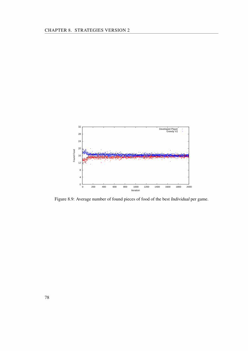
CHAPTER 8. STRATEGIES VERSION 2
0
4
8
12
16
20
24
28
32
0 200 400 600 800 1000 1200 1400 1600 1800 2000
Fou
nd F
ood
Iteration
Developed PlayerGreedy V2
Figure 8.9: Average number of found pieces of food of the best Individual per game.
78
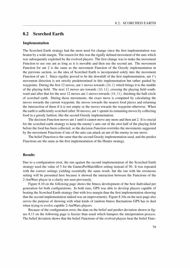
8.2. SCORCHED EARTH
8.2 Scorched Earth
Implementation
The Scorched Earth strategy had the most need for change since the first implementation wasbeaten by a wide margin. The reason for this was the rigidly defined movement of the ants whichwas subsequently exploited by the evolved players. The first change was to make the movementFunction to use one ant as long as it is movable and then use the second ant. The movementFunction for ant 2 is the same as the movement Function of the Greedy implementation inthe previous section, so the idea of Scorched Earth is incorporated solely into the movementFunction of ant 1. Since rigidity proved to be the downfall of the first implementation, ant 1’smovement direction is not strictly predetermined in this implementation but rather guided bywaypoints. During the first 12 moves, ant 1 moves towards (10, 1) which brings it to the middleof the playing field. The next 12 moves are towards (10, 11), crossing the playing field south-ward and after that for the next 12 moves ant 1 moves towards (18, 11), finishing the half-circleof scorched earth. During those movements, the exact move is computed by calculating themoves towards the current waypoint, the moves towards the nearest food pieces and returningthe intersection of them if it is not empty or the moves towards the waypoint otherwise. Whenthe earth is sufficiently scorched (after 36 moves), ant 1 spends its remaining moves by collectingfood in a greedy fashion, like the second Greedy implementation.
The decision Function moves ant 1 until it cannot move any more and then ant 2. It is crucialfor the scorched earth strategy to keep the enemy’s ants out of the own half of the playing fieldbefore the food has been collected, so the decision Function overrides the movements suggestedby the movement Functions if one of the ants can attack an ant of the enemy in one move.
The belief Function is the same that the second Greedy implementation used, and the predictFunctions are the same as the first implementation of the Hunter strategy.
Results
Due to a configuration error, the run against the second implementation of the Scorched Earthstrategy used the value of 5 for the GamesPerMatchBest setting instead of 50. It was repeatedwith the correct settings yielding essentially the same result, but the run with the erroneoussetting will be presented here because it showed the interaction between the Functions of the2-AntWars player in a clarity not seen previously.
Figure 8.10 on the following page shows the fitness development of the best Individual pergeneration for both configurations. In both runs, GPS was able to develop players capable ofbeating the Scorched Earth strategy (but with less margin than the first implementation showingthat the second implementation indeed was an improvement). Figure 8.10a on the next page alsoserves the purpose of showing with what kinds of random fitness fluctuations GPS has to dealwhen trying to evolve capable 2-AntWars players.
Because of the configuration error, the data on the belief and predict deviation shown in fig-ure 8.11 on the following page is fuzzier than usual which hampers the interpretation process.The belief deviation shows that the belief Functions of the evolved players beat the belief Func-
79

CHAPTER 8. STRATEGIES VERSION 2
0
4
8
12
16
20
24
28
32
0 100 200 300 400 500 600 700 800 900 1000
Fou
nd F
ood
Iteration
Developed PlayerScorched Earth V2
(a) Erroneous 5 GamesPerMatchBest
0
4
8
12
16
20
24
28
32
0 100 200 300 400 500 600 700 800 900 1000
Fou
nd F
ood
Iteration
Developed PlayerScorched Earth V2
(b) Correct 50 GamesPerMatchBest
Figure 8.10: Average number of found pieces of food of the best Individual per game, (a) withonly five games between the best Individual and the Scorched Earth strategy and (b) the correctamount of games between them.
0
200
400
600
800
1000
0 100 200 300 400 500 600 700 800 900 1000
Bel
ief D
evia
tion
Iteration
Developed PlayerScorched Earth V2
(a) Belief deviation
0
1000
2000
3000
4000
5000
6000
7000
0 100 200 300 400 500 600 700 800 900 1000
Pre
dict
Dev
iatio
n
Iteration
Developed Player predict0Developed Player predict1
Scorched Earth V2 predict0Scorched Earth V2 predict1
(b) Predict deviation
Figure 8.11: Average belief and predict deviations of the best Individual and its opponent pergame.
tion of the Scorched Earth player. Note the improvement of the evolved belief Function aroundgeneration 800, this will come into play later.
The belief Function that the best Individual of the last generation uses showed the mostcomplex behaviour of all the belief Functions discussed until now. It believes in seen foodconstantly with a value of one. Initially, it also believes in unseen food with the same value.After 20 moves, the belief in food at unseen positions only remains in the seven rows on thetop of the playing field and it shrinks to two rows after 40 moves. This is a result of the factthat ant 1 of the Scorched Earth player misses more food at the begin of his arc than at the end(because at the end it greedily collects food in the area at the bottom of the playing field). Afterant 1 has exhausted its moves, ant 2 collects food around its starting position in the center areaof the playing field, leaving only the top most rows unharvested (with a certain probability, notalways). The downside of this is that food in the south-western corner of the playing field goes
80

8.2. SCORCHED EARTH
0
100
200
300
400
500
600
700
800
900
1000
0 100 200 300 400 500 600 700 800 900 1000
Indi
vidu
al
Iteration
0
20
40
60
80
100
120
A
B
C
Figure 8.12: Found food of the Individuals playing 2-AntWars against a Scorched Earth player.
0
100
200
300
400
500
600
700
800
900
1000
0 100 200 300 400 500 600 700 800 900 1000
Indi
vidu
al
Iteration
0
1000
2000
3000
4000
5000
B
Figure 8.13: Belief deviation of the Individuals playing 2-AntWars against a Scorched Earthplayer.
uneaten by the evolved players because they evolved in a way that lets them be guided by thefood belief but not by unseen fields and it is too far away for ant 2 of the Scorched Earth player.
The predict Functions did not evolve this kind of behavioural complexity. The prediction ofant 1 moves to (12, 6) and then jumps around in a one move neighborhood around it which is agood approximation of the later positions of ant 1. The prediction of ant 2 stays at the positionone move to the west of ant 2’s starting position.
The fitness development of the population depicted in figure 8.12 shows fairly standard be-haviour during the first 500 generations, with species A taking over the population. A obviouslyconsists of multiple subspecies but this is not the focus of concern right now. What’s impor-tant is spawn point B, where it seems that a species with inferior fitness emerged that spreadthroughout the whole population. Only some time later, another species reestablished the fitness
81

CHAPTER 8. STRATEGIES VERSION 2
0
5
10
15
20
25
0 100 200 300 400 500 600 700 800 900 1000
Fou
nd F
ood
Iteration
0
20
40
60
80
100
120
(a) Ant 1
0
5
10
15
20
25
0 100 200 300 400 500 600 700 800 900 1000
Fou
nd F
ood
Iteration
0
20
40
60
80
100
120
(b) Ant 2
Figure 8.14: Distribution of average found food per ant and game against a Scorched Earthplayer.
0
100
200
300
400
500
600
700
800
900
1000
0 100 200 300 400 500 600 700 800 900 1000
Indi
vidu
al
Iteration
0
10
20
30
40
50
60
70
80
B
Figure 8.15: Average time when both ants of the Individuals playing 2-AntWars leave theirstarting positions against a Scorched Earth player.
level of A at spawn point C. Here figure 8.11a on page 80 comes to mind as it showed that thebest Individuals of the population began to use improved belief Functions around generation800 which is also the same time C emerges. This indicates that an improvement in the beliefFunction might be responsible for the inferior species B.
Figure 8.13 on the previous page shows the development of the belief deviation of the pop-ulation and indeed, spawnpoint B marks the rise of a new and improved belief Function. It be-haved differently than its predecessor and damaged the performance of the evolved 2-AntWarsplayers, but what exactly changed? The performance of ant 1 (figure 8.14a) was influenced,while the one of ant 2 (figure 8.14b) stayed constant. Figure 8.15 shows the average time whenboth ants of the developed player have left the starting positions. Note that B is visible, but not asusual for this graph where new species show up by moving both ants before the player moved 40times. Instead, the ants of B take more than 40 moves on average to leave their starting positions.
82

8.2. SCORCHED EARTH
0
20
40
60
80
100
120
140
0 100 200 300 400 500 600 700 800 900 1000
Fou
nd F
ood
Iteration
0
10
20
30
40
50
60
(a) Distribution of found food
0
0.1
0.2
0.3
0.4
0.5
0.6
0.7
0.8
0 100 200 300 400 500 600 700 800 900 1000
Mat
ch W
in P
roba
bilit
y
Iteration
(b) Probability of winning a match
Figure 8.16: (a) Distribution of found food and (b) probability of winning a match against aScorched Earth player.
This can happen in two ways. The first way is that ant 1 (which is the ant that moves second)might wait some moves after ant 2 ran out of moves before it starts moving, which seems un-likely. The second possibility is that in some cases ant 1 moves immediately after ant 2 ran outof moves, but in some cases does not move at all. This can happen when the belief Functiondoes not believe in food at unseen positions, the player has not seen food that he has not eatenand does not explore unseen fields. That seems to be the reason for the less fit individuals.
Note also how this figure shows the existence of additional species that move both of theirants earlier, confirming the previous assertion that A consists of multiple species.
The fitness distribution of the Individuals in the population (figure 8.16a) shows the damagedone by the emergence of the improved belief Function at B. It is even more visible in fig-ure 8.16b, with the probability of winning a match dipping from 0.6 to 0.5. The run with thecorrect settings did not have this dip and the probability of winning converged to 0.7. Also notethat the whole population reaches a win probability of 0.5 after 400 generations while the bestIndividuals start beating the Scorched Earth player after 100 generations.
In this run, the population size rose only to 500000 Statements instead of the 600000 State-ments seen previously. The time needed to evaluate a generation also diverged from the stan-dard behaviour, it decreased from 120 to 100 seconds during the first 500 generations but thenincreased, reaching 120 again at the end of the run.
83

CHAPTER 8. STRATEGIES VERSION 2
8.3 Hunter
Implementation
It was hard for GPS to evolve players that beat the first implementation of the Hunter strategy,so the improved implementation of the Hunter kept the separation of concern between huntingant and gathering ant and was made even more aggressive and focused on one target.
The base of movement, the implementation of the movement Functions, reused the move-ment Function of the second implementation of the Greedy player so it would benefit from itsimprovements.
The decision Function was still the centerpiece of the hunting behaviour, because it hasaccess to the position predictions of the enemy’s ants. The first step of the decision Functionis checking if one of the ants is one move away from one of the ants of the enemy, if so, theant will attack. Otherwise the Moves towards both of the enemy’s ants are calculated. If theintersection is not empty, the intersection is used as the base for the further decision process. Inthe case that the intersection is empty, the Moves towards the nearest (or the union of the Movesif the distance is the same) is used as the base. If the intersection of the base with the Moves-suggestion of movement1 is not empty, the result is used to override the Moves-suggestion forant 1, otherwise the base overrides the Moves-suggestion and the ID of ant 1 is returned. Thiscalculation is only done if ant 1 is actually movable, in the case that it is not, the ID of ant 2 isreturned.
The belief and predict Functions work exactly like they did in the first implementation of theHunter strategy.
Results
The run against the second implementation of the Hunter strategy was not successful as is shownby figure 8.17a on the next page. Around generation 720 the evolved players were finally ableto catch up but not competent enough to actually beat the Hunter strategy. The problem was thatthe evolved players did not use both ants effectively until this jump in fitness around generation720, so the run was repeated with a population size of 2000 and 2000 generations. The resultsof this run are presented here.
Figure 8.17b on the facing page shows the result of the run with changed settings against theHunter strategy. In this run, the best Individuals were on par with the Hunter player after 1000,and able to beat it after 2000 generations.
The belief Functions of the developed player were not able to beat the belief Function ofthe Hunter player until generation 1600 (figure 8.18a on the next page). Beginning with thatgeneration a transition to a better performing belief Function can be witnessed, so even thoughthe run had already lasted for 1600 generations, there were still improvements found. The beliefFunction of the best Individual of the last generation always believes in food that was once seenand in food at unseen positions until the 31-st move, when it only believes in food at unseenpositions at the two northern-most rows of the playing field. This is a good approximation ofthe behaviour of the Hunter, because the hunting ant will go most likely straight west and thegathering ant starts in the southern half of the playing field.
84

8.3. HUNTER
0
4
8
12
16
20
24
28
32
0 100 200 300 400 500 600 700 800 900 1000
Fou
nd F
ood
Iteration
Developed PlayerHunter V2
(a) Normal settings
0
4
8
12
16
20
24
28
32
0 200 400 600 800 1000 1200 1400 1600 1800 2000
Fou
nd F
ood
Iteration
Developed PlayerHunter V2
(b) Large population
Figure 8.17: Average number of found pieces of food of the best Individual per game, (a) withthe normal settings and (b) with 2000 iterations and 2000 Individuals.
0
200
400
600
800
1000
0 200 400 600 800 1000 1200 1400 1600 1800 2000
Bel
ief D
evia
tion
Iteration
Developed PlayerHunter V2
(a) Belief deviation
0
500
1000
1500
2000
2500
3000
3500
4000
0 200 400 600 800 1000 1200 1400 1600 1800 2000
Pre
dict
Dev
iatio
n
Iteration
Developed Player predict0Developed Player predict1
Hunter V2 predict0Hunter V2 predict1
(b) Predict deviation
Figure 8.18: Average belief and predict deviations of the best Individual and its opponent pergame.
The predict Functions (figure 8.18b) showed much more prediction precision than the onesof the Hunter and was doing better with the prediction of the hunting ant because its generaldirection is constant. The prediction Function for ant 1 of the best Individual in the last gener-ation moved the prediction one step west with each move and stopped at (5, 5). The predictionFunction for ant 2 kept the prediction at the starting position until the 34-th move, when it wasset to (14, 8). Note that the prediction Function of the Hunter worked worse than in the run withthe previous implementation, even though they are identical which indicates that the evolvedplayers move their ants in a way very contrary to the expectations of the predict Functions of theHunter. This seems logical as the hunting ant bases its movement decisions on these predictionsand the evolved player’s ants do not want to be found and attacked.
The development of the found food per match depicted in figure 8.19 on the next page israther unremarkable. After 700 generations the species in the population seem to have con-verged, some variation in fitness level can be seen but not enough to separate different species.
85

CHAPTER 8. STRATEGIES VERSION 2
0
200
400
600
800
1000
1200
1400
1600
1800
2000
0 200 400 600 800 1000 1200 1400 1600 1800 2000
Indi
vidu
al
Iteration
0
20
40
60
80
100
120
Figure 8.19: Found food of the Individuals playing 2-AntWars against a Hunter player.
0
20
40
60
80
100
120
140
0 200 400 600 800 1000 1200 1400 1600 1800 2000
Fou
nd F
ood
Iteration
0
10
20
30
40
50
60
70
80
(a) Distribution of found food
0
0.1
0.2
0.3
0.4
0.5
0 200 400 600 800 1000 1200 1400 1600 1800 2000
Mat
ch W
in P
roba
bilit
y
Iteration
(b) Probability of winning a match
Figure 8.20: (a) Distribution of found food and (b) probability of winning a match against aHunter player.
Another insight into the fitness development can be gained by studying figures 8.20aand 8.20b. There is only one dominant level of fitness present in the population as it slowlyimproves. The probability of winning a game improves by 10 percent between generations 1000and 2000, a fact which is completely invisible in figure 8.19.
Figure 8.21 on the next page shows how the ants of the players contribute to the final fitness.It can be seen immediately that the division of labour between the ants of player 1 (the developedplayer) is completely different when compared to the previous runs. In this run, both ants con-tributed equally to the total amount of found food while in previous runs one ant was dominant,moved first and collected most of the food while the second ant searched for the missed piecesof food. Also interesting is the fact that the hunting ant (ant 1 of player 2) collects more foodthan the gathering ant, simply because it moves first and has more opportunity to do so.
Now the obvious question is what the developed player was doing with his ants to reach thisequal distribution of found food between the ants. The next figures shed light on this subject.
86

8.3. HUNTER
0
5
10
15
20
25
0 200 400 600 800 1000 1200 1400 1600 1800 2000
Fou
nd F
ood
Iteration
0
50
100
150
200
250
(a) Player 1 Ant 1
0
5
10
15
20
25
0 200 400 600 800 1000 1200 1400 1600 1800 2000
Fou
nd F
ood
Iteration
0
50
100
150
200
250
(b) Player 1 Ant 2
0
5
10
15
20
25
0 200 400 600 800 1000 1200 1400 1600 1800 2000
Fou
nd F
ood
Iteration
0
50
100
150
200
250
(c) Player 2 Ant 1
0
5
10
15
20
25
0 200 400 600 800 1000 1200 1400 1600 1800 2000
Fou
nd F
ood
Iteration
0
50
100
150
200
250
(d) Player 2 Ant 2
Figure 8.21: Distribution of average found food per ant and game against a Hunter player.
0
200
400
600
800
1000
1200
1400
1600
1800
2000
0 200 400 600 800 1000 1200 1400 1600 1800 2000
Indi
vidu
al
Iteration
0
10
20
30
40
50
60
70
80
Figure 8.22: Average time when both ants ofthe Individuals playing 2-AntWars leave theirstarting positions against a Hunter player.
0
200
400
600
800
1000
1200
1400
1600
1800
2000
0 200 400 600 800 1000 1200 1400 1600 1800 2000
Indi
vidu
al
Iteration
0
0.2
0.4
0.6
0.8
1
Figure 8.23: Probability of choosing ant 1 formovement.
87
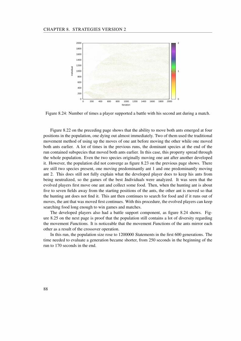
CHAPTER 8. STRATEGIES VERSION 2
0
200
400
600
800
1000
1200
1400
1600
1800
2000
0 200 400 600 800 1000 1200 1400 1600 1800 2000
Indi
vidu
al
Iteration
0
1
2
Figure 8.24: Number of times a player supported a battle with his second ant during a match.
Figure 8.22 on the preceding page shows that the ability to move both ants emerged at fourpositions in the population, one dying out almost immediately. Two of them used the traditionalmovement method of using up the moves of one ant before moving the other while one movedboth ants earlier. A lot of times in the previous runs, the dominant species at the end of therun contained subspecies that moved both ants earlier. In this case, this property spread throughthe whole population. Even the two species originally moving one ant after another developedit. However, the population did not converge as figure 8.23 on the previous page shows. Thereare still two species present, one moving predominantly ant 1 and one predominantly movingant 2. This does still not fully explain what the developed player does to keep his ants frombeing neutralized, so the games of the best Individuals were analyzed. It was seen that theevolved players first move one ant and collect some food. Then, when the hunting ant is aboutfive to seven fields away from the starting positions of the ants, the other ant is moved so thatthe hunting ant does not find it. This ant then continues to search for food and if it runs out ofmoves, the ant that was moved first continues. With this procedure, the evolved players can keepsearching food long enough to win games and matches.
The developed players also had a battle support component, as figure 8.24 shows. Fig-ure 8.25 on the next page is proof that the population still contains a lot of diversity regardingthe movement Functions. It is noticeable that the movement Functions of the ants mirror eachother as a result of the crossover operation.
In this run, the population size rose to 1200000 Statements in the first 600 generations. Thetime needed to evaluate a generation became shorter, from 250 seconds in the beginning of therun to 170 seconds in the end.
88
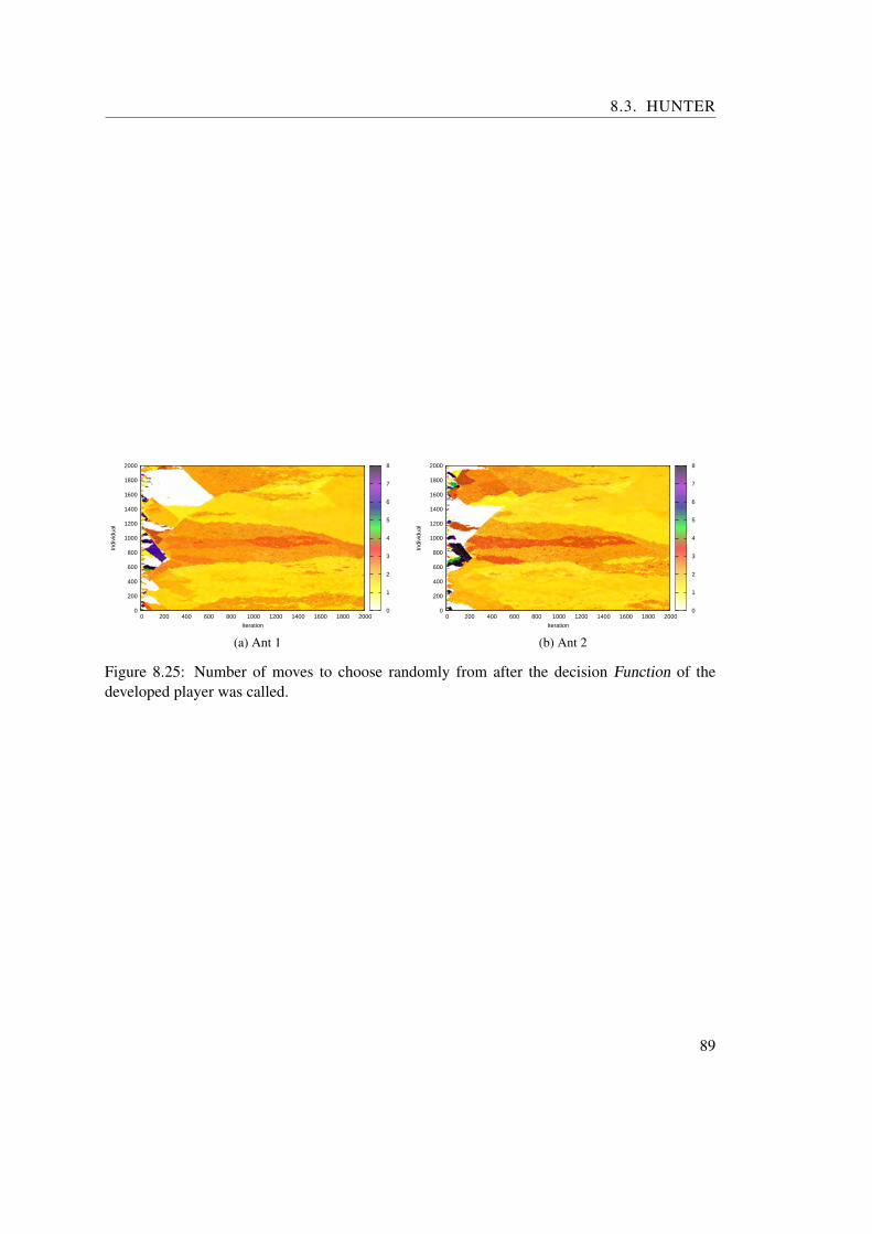
8.3. HUNTER
0
200
400
600
800
1000
1200
1400
1600
1800
2000
0 200 400 600 800 1000 1200 1400 1600 1800 2000
Indi
vidu
al
Iteration
0
1
2
3
4
5
6
7
8
(a) Ant 1
0
200
400
600
800
1000
1200
1400
1600
1800
2000
0 200 400 600 800 1000 1200 1400 1600 1800 2000
Indi
vidu
al
Iteration
0
1
2
3
4
5
6
7
8
(b) Ant 2
Figure 8.25: Number of moves to choose randomly from after the decision Function of thedeveloped player was called.
89


CHAPTER 9Coevolutionary Runs
This chapter details four coevolutionary runs, that means that both player 1 and player 2 weresubject to evolution. Section 9.1 reports on a coevolutionary run with the standard settings, whilesection 9.2 on page 97 presents the results of a run using asymmetric evaluation with a ∆eval of1. As a result, the Individuals in the host population are evaluated by playing three matchesagainst Individuals from the parasite population while only the result of one match is used toassign a score to the parasite Individuals.
The following two sections document runs where the aim was to explore the long termbehaviour of coevolution. Both runs used a population of 500 Individuals and more generoussize limits for the Functions of the 2-AntWars players (belief 200, predict 200, decision 300 andmovement 400 Statements). ∆host and ∆parasite were set to 2 instead of 3 because of the smallerpopulation. For every other setting (except the number of generations) the standard values wereused. Section 9.3 on page 101 presents a run with these settings over the course of 10000generations. The run that delivered the content of section 9.4 on page 104 used asymmetricevaluation with a ∆eval of 1. Originally it was planned to let GPS evolve players for 10000generations but due to the exorbitant time requirements the run was aborted after two weeks and6500 generations.
9.1 Run with Standard Settings
Figure 9.1 on the following page shows the average number of pieces of food the best Individualof the host population (playing as player 1) and the best Individual of the parasite population(playing as player 2) found on average during a game. It took player 2 200 generations to reachthe level of player 1 and from that generation on the performance of the players was about thesame. It seems, however, that player 1 has a slight advantage as there are more outliers withbetter performance than worse performance.
It has to be mentioned that this type of graph is only of limited significance in coevolutionaryruns because the best player 1 is most likely at a different position in the population than the bestplayer 2 so when each of them adapts to their opponents they do not adapt to each other. It is
91
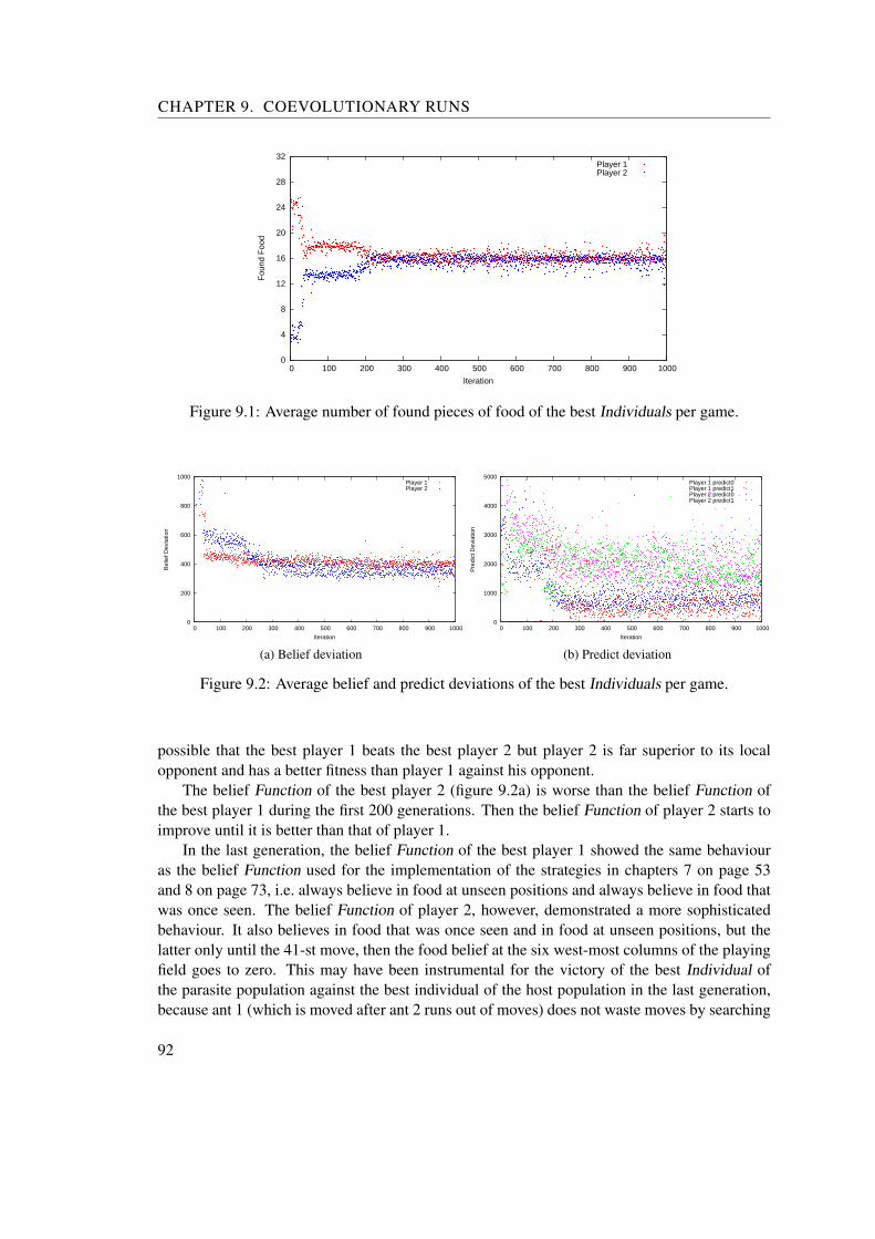
CHAPTER 9. COEVOLUTIONARY RUNS
0
4
8
12
16
20
24
28
32
0 100 200 300 400 500 600 700 800 900 1000
Fou
nd F
ood
Iteration
Player 1Player 2
Figure 9.1: Average number of found pieces of food of the best Individuals per game.
0
200
400
600
800
1000
0 100 200 300 400 500 600 700 800 900 1000
Bel
ief D
evia
tion
Iteration
Player 1Player 2
(a) Belief deviation
0
1000
2000
3000
4000
5000
0 100 200 300 400 500 600 700 800 900 1000
Pre
dict
Dev
iatio
n
Iteration
Player 1 predict0Player 1 predict1Player 2 predict0Player 2 predict1
(b) Predict deviation
Figure 9.2: Average belief and predict deviations of the best Individuals per game.
possible that the best player 1 beats the best player 2 but player 2 is far superior to its localopponent and has a better fitness than player 1 against his opponent.
The belief Function of the best player 2 (figure 9.2a) is worse than the belief Function ofthe best player 1 during the first 200 generations. Then the belief Function of player 2 starts toimprove until it is better than that of player 1.
In the last generation, the belief Function of the best player 1 showed the same behaviouras the belief Function used for the implementation of the strategies in chapters 7 on page 53and 8 on page 73, i.e. always believe in food at unseen positions and always believe in food thatwas once seen. The belief Function of player 2, however, demonstrated a more sophisticatedbehaviour. It also believes in food that was once seen and in food at unseen positions, but thelatter only until the 41-st move, then the food belief at the six west-most columns of the playingfield goes to zero. This may have been instrumental for the victory of the best Individual ofthe parasite population against the best individual of the host population in the last generation,because ant 1 (which is moved after ant 2 runs out of moves) does not waste moves by searching
92
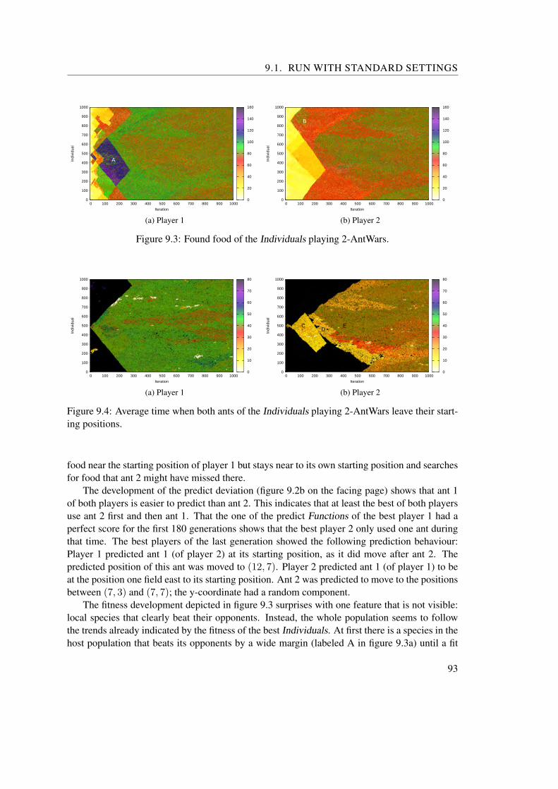
9.1. RUN WITH STANDARD SETTINGS
0
100
200
300
400
500
600
700
800
900
1000
0 100 200 300 400 500 600 700 800 900 1000
Indi
vidu
al
Iteration
0
20
40
60
80
100
120
140
160
A
(a) Player 1
0
100
200
300
400
500
600
700
800
900
1000
0 100 200 300 400 500 600 700 800 900 1000
Indi
vidu
al
Iteration
0
20
40
60
80
100
120
140
160
B
(b) Player 2
Figure 9.3: Found food of the Individuals playing 2-AntWars.
0
100
200
300
400
500
600
700
800
900
1000
0 100 200 300 400 500 600 700 800 900 1000
Indi
vidu
al
Iteration
0
10
20
30
40
50
60
70
80
(a) Player 1
0
100
200
300
400
500
600
700
800
900
1000
0 100 200 300 400 500 600 700 800 900 1000
Indi
vidu
al
Iteration
0
10
20
30
40
50
60
70
80
CD
E
(b) Player 2
Figure 9.4: Average time when both ants of the Individuals playing 2-AntWars leave their start-ing positions.
food near the starting position of player 1 but stays near to its own starting position and searchesfor food that ant 2 might have missed there.
The development of the predict deviation (figure 9.2b on the facing page) shows that ant 1of both players is easier to predict than ant 2. This indicates that at least the best of both playersuse ant 2 first and then ant 1. That the one of the predict Functions of the best player 1 had aperfect score for the first 180 generations shows that the best player 2 only used one ant duringthat time. The best players of the last generation showed the following prediction behaviour:Player 1 predicted ant 1 (of player 2) at its starting position, as it did move after ant 2. Thepredicted position of this ant was moved to (12, 7). Player 2 predicted ant 1 (of player 1) to beat the position one field east to its starting position. Ant 2 was predicted to move to the positionsbetween (7, 3) and (7, 7); the y-coordinate had a random component.
The fitness development depicted in figure 9.3 surprises with one feature that is not visible:local species that clearly beat their opponents. Instead, the whole population seems to followthe trends already indicated by the fitness of the best Individuals. At first there is a species in thehost population that beats its opponents by a wide margin (labeled A in figure 9.3a) until a fit
93
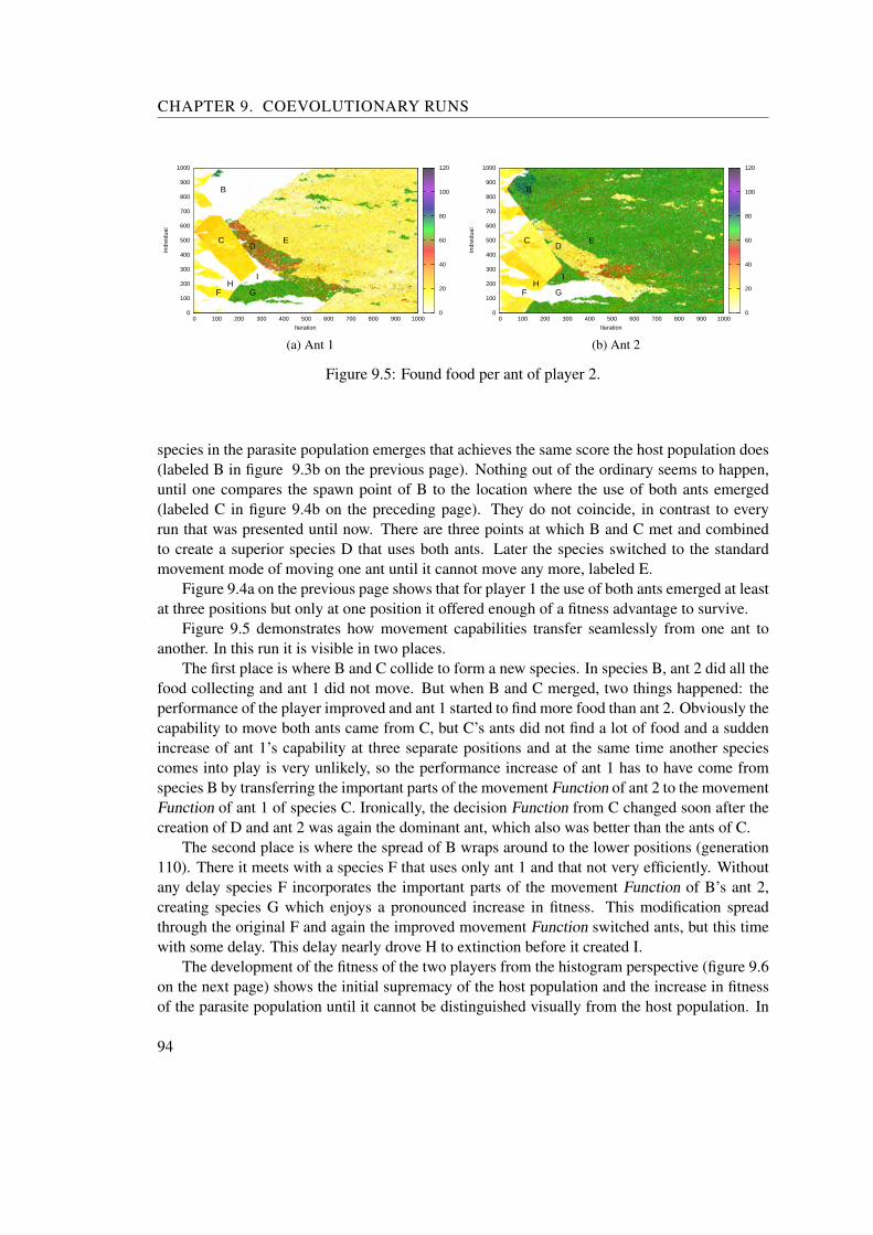
CHAPTER 9. COEVOLUTIONARY RUNS
0
100
200
300
400
500
600
700
800
900
1000
0 100 200 300 400 500 600 700 800 900 1000
Indi
vidu
al
Iteration
0
20
40
60
80
100
120
B
CD
E
F GH
I
(a) Ant 1
0
100
200
300
400
500
600
700
800
900
1000
0 100 200 300 400 500 600 700 800 900 1000
Indi
vidu
al
Iteration
0
20
40
60
80
100
120
B
CD
E
F GH
I
(b) Ant 2
Figure 9.5: Found food per ant of player 2.
species in the parasite population emerges that achieves the same score the host population does(labeled B in figure 9.3b on the previous page). Nothing out of the ordinary seems to happen,until one compares the spawn point of B to the location where the use of both ants emerged(labeled C in figure 9.4b on the preceding page). They do not coincide, in contrast to everyrun that was presented until now. There are three points at which B and C met and combinedto create a superior species D that uses both ants. Later the species switched to the standardmovement mode of moving one ant until it cannot move any more, labeled E.
Figure 9.4a on the previous page shows that for player 1 the use of both ants emerged at leastat three positions but only at one position it offered enough of a fitness advantage to survive.
Figure 9.5 demonstrates how movement capabilities transfer seamlessly from one ant toanother. In this run it is visible in two places.
The first place is where B and C collide to form a new species. In species B, ant 2 did all thefood collecting and ant 1 did not move. But when B and C merged, two things happened: theperformance of the player improved and ant 1 started to find more food than ant 2. Obviously thecapability to move both ants came from C, but C’s ants did not find a lot of food and a suddenincrease of ant 1’s capability at three separate positions and at the same time another speciescomes into play is very unlikely, so the performance increase of ant 1 has to have come fromspecies B by transferring the important parts of the movement Function of ant 2 to the movementFunction of ant 1 of species C. Ironically, the decision Function from C changed soon after thecreation of D and ant 2 was again the dominant ant, which also was better than the ants of C.
The second place is where the spread of B wraps around to the lower positions (generation110). There it meets with a species F that uses only ant 1 and that not very efficiently. Withoutany delay species F incorporates the important parts of the movement Function of B’s ant 2,creating species G which enjoys a pronounced increase in fitness. This modification spreadthrough the original F and again the improved movement Function switched ants, but this timewith some delay. This delay nearly drove H to extinction before it created I.
The development of the fitness of the two players from the histogram perspective (figure 9.6on the next page) shows the initial supremacy of the host population and the increase in fitnessof the parasite population until it cannot be distinguished visually from the host population. In
94

9.1. RUN WITH STANDARD SETTINGS
0
20
40
60
80
100
120
140
0 100 200 300 400 500 600 700 800 900 1000
Fou
nd F
ood
Iteration
0
10
20
30
40
50
(a) Player 1
0
20
40
60
80
100
120
140
0 100 200 300 400 500 600 700 800 900 1000
Fou
nd F
ood
Iteration
0
10
20
30
40
50
(b) Player 2
Figure 9.6: Fitness distribution.
0
0.1
0.2
0.3
0.4
0.5
0.6
0.7
0.8
0.9
1
0 100 200 300 400 500 600 700 800 900 1000
Mat
ch W
in P
roba
bilit
y
Iteration
Player 1Player 2
Tie
Figure 9.7: Probability of winning a match.
the last 20 generations, every Individual of the host population found 79.44 pieces of food, whilethe Individuals of the parasite population found 76.28 pieces on average.
Figure 9.7 shows the probability of a random player of the host and parasite populationwinning a match. The first short-lived increase in win probability of player 2 coincides withthe emergence of species B. It clearly can be seen that the probability of winning the matchfor player 2 does not reach the probability for player 1. Note that as the winning probabilitiesdraw closer, the probability of a tie increases, which was 2% at the end of the run. The increaseof winning probability for player 1 around generation 900 was not visible in any of the othergraphs so it is not clear what caused it. It is, however, noteworthy that if the host populationincreased its fitness by changing its behaviour, the parasite population was able to adapt fast toreach the previous fitness levels. If the change was caused by some sort of defect in the parasitepopulation, it was corrected fast. Whatever the cause, it does suggest stable populations andperformance levels.
95

CHAPTER 9. COEVOLUTIONARY RUNS
No species in both parts of the population evolved any kind of aggressiveness, there were ofcourse some battles but they were more like accidents when the ants crossed paths than deliberatechoices to fight. Similarly no support in battle evolved.
The fact that this and the following runs used coevolution had no influence on the qualitativecharacteristics of the population size and execution time. The population size doubled becausethe number of Individuals doubled. The execution time did not double because even with normalevolution some player 2 had to be executed every game. Again the execution time showed nocorrelation to the size of the population.
0
200000
400000
600000
800000
1e+06
1.2e+06
0 100 200 300 400 500 600 700 800 900 1000
Pop
ulat
ion
Siz
e [#
Sta
tem
ents
]
Iteration
(a)
0
20
40
60
80
100
120
140
0 100 200 300 400 500 600 700 800 900 1000
CP
U T
ime
[s]
Iteration
(b)
Figure 9.8: (a) Total number of Statements contained in the population and (b) the time neededto evaluate them.
96

9.2. RUN WITH ASYMMETRIC EVALUATION
0
4
8
12
16
20
24
28
32
0 100 200 300 400 500 600 700 800 900 1000
Fou
nd F
ood
Iteration
Player 1Player 2
Figure 9.9: Average number of found pieces of food of the best Individual per game.
0
200
400
600
800
1000
0 100 200 300 400 500 600 700 800 900 1000
Bel
ief D
evia
tion
Iteration
Player 1Player 2
(a) Belief deviation
0
1000
2000
3000
4000
5000
6000
0 100 200 300 400 500 600 700 800 900 1000
Pre
dict
Dev
iatio
n
Iteration
Player 1 predict0Player 1 predict1Player 2 predict0Player 2 predict1
(b) Predict deviation
Figure 9.10: Average belief and predict deviations of the best Individual and its opponent pergame.
9.2 Run with Asymmetric Evaluation
The expectation for the run with asymmetric evaluation was that player 1 would beat player 2because he gets three times more evaluation information and GPS can better select the fitterIndividuals. The run, however, did not turn out that way. Figure 9.9 shows the results of thebattle between the best player 1 and the best player 2. Player 2 consistently beats player 1 by aconvincing margin. Player 2 was able to do that after it developed the efficient use of both ants.
The deviation of the belief Functions in figure 9.10a shows that the best Individuals of theparasite population start using an improved version beginning with the 800-th generation. Thisimproved belief Function initially believes in food at unseen positions and that food once seenis never eaten by the enemy’s ants. After some moves, however, the belief Function reduces thebelief at the west-most column of the playing field to zero. Every two moves on average thewest-most column that still believes in food at unseen positions has its belief reduced to zero.
97
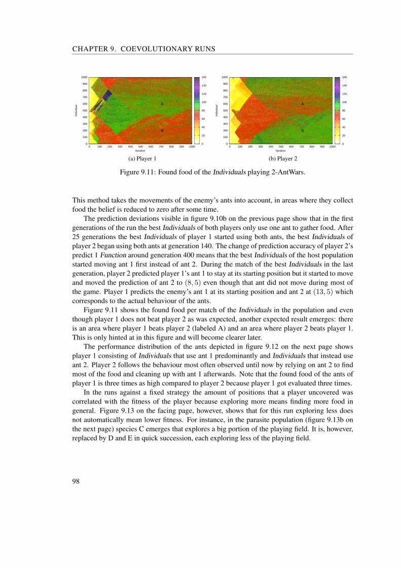
CHAPTER 9. COEVOLUTIONARY RUNS
0
100
200
300
400
500
600
700
800
900
1000
0 100 200 300 400 500 600 700 800 900 1000
Indi
vidu
al
Iteration
0
20
40
60
80
100
120
140
160
A
B
(a) Player 1
0
100
200
300
400
500
600
700
800
900
1000
0 100 200 300 400 500 600 700 800 900 1000
Indi
vidu
al
Iteration
0
20
40
60
80
100
120
140
160
A
B
(b) Player 2
Figure 9.11: Found food of the Individuals playing 2-AntWars.
This method takes the movements of the enemy’s ants into account, in areas where they collectfood the belief is reduced to zero after some time.
The prediction deviations visible in figure 9.10b on the previous page show that in the firstgenerations of the run the best Individuals of both players only use one ant to gather food. After25 generations the best Individuals of player 1 started using both ants, the best Individuals ofplayer 2 began using both ants at generation 140. The change of prediction accuracy of player 2’spredict 1 Function around generation 400 means that the best Individuals of the host populationstarted moving ant 1 first instead of ant 2. During the match of the best Individuals in the lastgeneration, player 2 predicted player 1’s ant 1 to stay at its starting position but it started to moveand moved the prediction of ant 2 to (8, 5) even though that ant did not move during most ofthe game. Player 1 predicts the enemy’s ant 1 at its starting position and ant 2 at (13, 5) whichcorresponds to the actual behaviour of the ants.
Figure 9.11 shows the found food per match of the Individuals in the population and eventhough player 1 does not beat player 2 as was expected, another expected result emerges: thereis an area where player 1 beats player 2 (labeled A) and an area where player 2 beats player 1.This is only hinted at in this figure and will become clearer later.
The performance distribution of the ants depicted in figure 9.12 on the next page showsplayer 1 consisting of Individuals that use ant 1 predominantly and Individuals that instead useant 2. Player 2 follows the behaviour most often observed until now by relying on ant 2 to findmost of the food and cleaning up with ant 1 afterwards. Note that the found food of the ants ofplayer 1 is three times as high compared to player 2 because player 1 got evaluated three times.
In the runs against a fixed strategy the amount of positions that a player uncovered wascorrelated with the fitness of the player because exploring more means finding more food ingeneral. Figure 9.13 on the facing page, however, shows that for this run exploring less doesnot automatically mean lower fitness. For instance, in the parasite population (figure 9.13b onthe next page) species C emerges that explores a big portion of the playing field. It is, however,replaced by D and E in quick succession, each exploring less of the playing field.
98

9.2. RUN WITH ASYMMETRIC EVALUATION
0
10
20
30
40
50
60
70
0 100 200 300 400 500 600 700 800 900 1000
Fou
nd F
ood
Iteration
0
10
20
30
40
50
60
(a) Player 1 Ant 1
0
10
20
30
40
50
60
70
0 100 200 300 400 500 600 700 800 900 1000
Fou
nd F
ood
Iteration
0
10
20
30
40
50
60
(b) Player 1 Ant 2
0
5
10
15
20
25
0 100 200 300 400 500 600 700 800 900 1000
Fou
nd F
ood
Iteration
0
20
40
60
80
100
(c) Player 2 Ant 1
0
5
10
15
20
25
0 100 200 300 400 500 600 700 800 900 1000
Fou
nd F
ood
Iteration
0
20
40
60
80
100
(d) Player 2 Ant 2
Figure 9.12: Average found food per ant and game.
0
100
200
300
400
500
600
700
800
900
1000
0 100 200 300 400 500 600 700 800 900 1000
Indi
vidu
al
Iteration
0
20
40
60
80
100
120
140
160
180
200
220
240
260
(a) Player 1
0
100
200
300
400
500
600
700
800
900
1000
0 100 200 300 400 500 600 700 800 900 1000
Indi
vidu
al
Iteration
0
20
40
60
80
100
120
140
160
180
200
220
240
260
C
DE
(b) Player 2
Figure 9.13: Average seen positions per game.
Figure 9.14 on the following page shows with more clarity what the fitness developmentof the population already suggested: two sections in the population, in one section player 1 isdominant, in one section player 2 is dominant. The sections are not stable, B slowly takes overthe population and A does not find a way to beat it. Note that the data of player 1 is based onthree matches but the data of player 2 on one match because of the asymmetric evaluation.
99
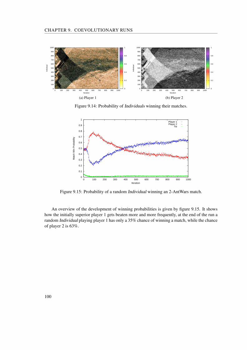
CHAPTER 9. COEVOLUTIONARY RUNS
0
100
200
300
400
500
600
700
800
900
1000
0 100 200 300 400 500 600 700 800 900 1000
Indi
vidu
al
Iteration
0
0.2
0.4
0.6
0.8
1
A
B
(a) Player 1
0
100
200
300
400
500
600
700
800
900
1000
0 100 200 300 400 500 600 700 800 900 1000
Indi
vidu
al
Iteration
0
0.2
0.4
0.6
0.8
1
A
B
(b) Player 2
Figure 9.14: Probability of Individuals winning their matches.
0
0.1
0.2
0.3
0.4
0.5
0.6
0.7
0.8
0.9
1
0 100 200 300 400 500 600 700 800 900 1000
Mat
ch W
in P
roba
bilit
y
Iteration
Player 1Player 2
Tie
Figure 9.15: Probability of a random Individual winning an 2-AntWars match.
An overview of the development of winning probabilities is given by figure 9.15. It showshow the initially superior player 1 gets beaten more and more frequently, at the end of the run arandom Individual playing player 1 has only a 35% chance of winning a match, while the chanceof player 2 is 63%.
100
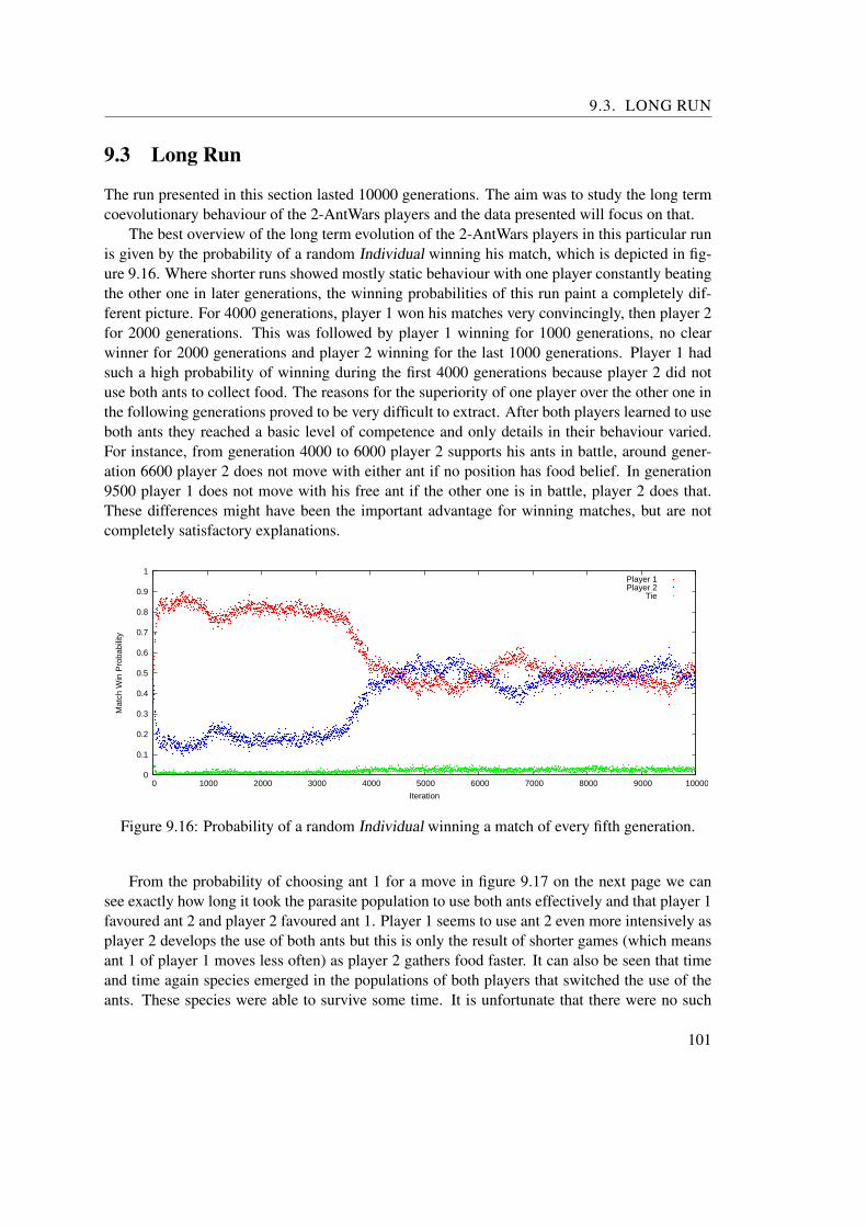
9.3. LONG RUN
9.3 Long Run
The run presented in this section lasted 10000 generations. The aim was to study the long termcoevolutionary behaviour of the 2-AntWars players and the data presented will focus on that.
The best overview of the long term evolution of the 2-AntWars players in this particular runis given by the probability of a random Individual winning his match, which is depicted in fig-ure 9.16. Where shorter runs showed mostly static behaviour with one player constantly beatingthe other one in later generations, the winning probabilities of this run paint a completely dif-ferent picture. For 4000 generations, player 1 won his matches very convincingly, then player 2for 2000 generations. This was followed by player 1 winning for 1000 generations, no clearwinner for 2000 generations and player 2 winning for the last 1000 generations. Player 1 hadsuch a high probability of winning during the first 4000 generations because player 2 did notuse both ants to collect food. The reasons for the superiority of one player over the other one inthe following generations proved to be very difficult to extract. After both players learned to useboth ants they reached a basic level of competence and only details in their behaviour varied.For instance, from generation 4000 to 6000 player 2 supports his ants in battle, around gener-ation 6600 player 2 does not move with either ant if no position has food belief. In generation9500 player 1 does not move with his free ant if the other one is in battle, player 2 does that.These differences might have been the important advantage for winning matches, but are notcompletely satisfactory explanations.
0
0.1
0.2
0.3
0.4
0.5
0.6
0.7
0.8
0.9
1
0 1000 2000 3000 4000 5000 6000 7000 8000 9000 10000
Mat
ch W
in P
roba
bilit
y
Iteration
Player 1Player 2
Tie
Figure 9.16: Probability of a random Individual winning a match of every fifth generation.
From the probability of choosing ant 1 for a move in figure 9.17 on the next page we cansee exactly how long it took the parasite population to use both ants effectively and that player 1favoured ant 2 and player 2 favoured ant 1. Player 1 seems to use ant 2 even more intensively asplayer 2 develops the use of both ants but this is only the result of shorter games (which meansant 1 of player 1 moves less often) as player 2 gathers food faster. It can also be seen that timeand time again species emerged in the populations of both players that switched the use of theants. These species were able to survive some time. It is unfortunate that there were no such
101

CHAPTER 9. COEVOLUTIONARY RUNS
0
100
200
300
400
500
0 1000 2000 3000 4000 5000 6000 7000 8000 9000 10000
Indi
vidu
al
Iteration
0
0.2
0.4
0.6
0.8
1
(a) Player 1
0
100
200
300
400
500
0 1000 2000 3000 4000 5000 6000 7000 8000 9000 10000
Indi
vidu
al
Iteration
0
0.2
0.4
0.6
0.8
1
(b) Player 2
Figure 9.17: Probability of choosing ant 1 for a move.
switched species at the same time and location in both populations, maybe then they could havesurvived. This is based on the assumption that moving first with the same ant as the opponent isa disadvantage because of a higher risk of running into the opponent’s ant.
Previous runs showed how the population size developed over time, and this run was noexception. Figure 9.18 on the facing page permits to gain insight into the size development ofIndividuals in the populations. Surprisingly, the populations diverged in terms of maximum size.Player 1’s population was saturated with large Individuals while large sections of player 2’s pop-ulation contained medium sized Individuals, even after the use of both ants developed (whichneeds bigger Individuals). Normally one would expect both populations to behave in a similarway because they are manipulated in the same manner. The only difference is the actual com-position of Individuals, so the structure of the Individuals might play a more important role forcode bloat than previously thought.
102
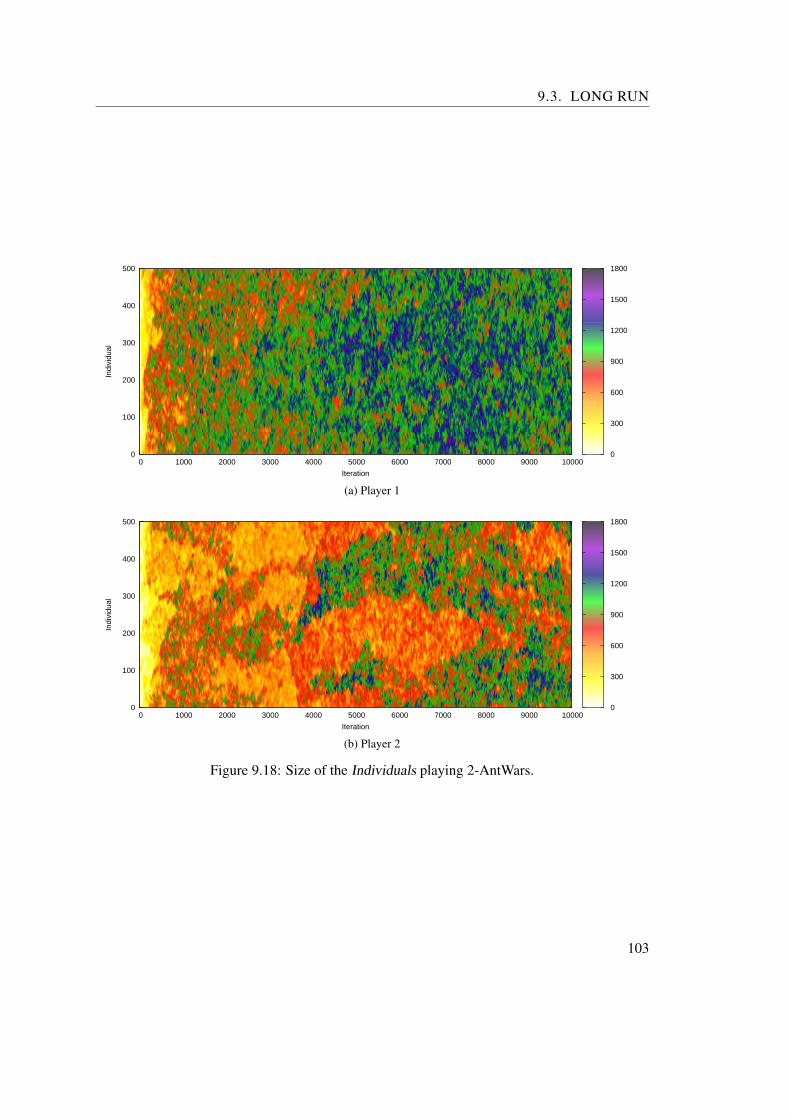
9.3. LONG RUN
0
100
200
300
400
500
0 1000 2000 3000 4000 5000 6000 7000 8000 9000 10000
Indi
vidu
al
Iteration
0
300
600
900
1200
1500
1800
(a) Player 1
0
100
200
300
400
500
0 1000 2000 3000 4000 5000 6000 7000 8000 9000 10000
Indi
vidu
al
Iteration
0
300
600
900
1200
1500
1800
(b) Player 2
Figure 9.18: Size of the Individuals playing 2-AntWars.
103

CHAPTER 9. COEVOLUTIONARY RUNS
9.4 Long Run with Asymmetric Evaluation
This section presents the long term evolutionary development of a run spanning 6500 generationswith asymmetric evaluation.
Figure 9.19 shows the probability of a random Individual winning a match. Once again thepopulation did not converge to stable performance levels, both players fought for superiorityinstead. The actual reasons as to why one player was better than the other one proved to beelusive. The initial advantage of player 1 was due to the fact that it took player 2 200 generationsto develop the use of both ants. During the rest of the run the belief Function and the adaptionof the movement and decision Functions seemed to be pivotal to the superiority of one playerover the other. The analysis of the games of the best Individuals of generation 1004 showed thatthe belief Function of player 1 switched the belief in food on unseen positions very early to zeroand his ants stopped moving because of that, which gave player 2 a significant advantage. Ingeneration 4500 the situation was reversed, player 2 was hindered by absent food belief at unseenpositions. At the end of the run, player 2 regained the upper hand by using a belief Function thatset the food belief from the forth to the seventh row from the top of the playing field to zero after13 moves. This corresponds to the immediate surroundings of ant 2 of player 1. The section ofzero belief grew larger until only the top-most and bottom-most row had food belief remaining.This has the effect that when an ant has explored one of the rows in search of food it traverses theplaying field to explore the other row. During the traversal the ant has a chance to find food thatit does not believe in. This chance would not be present if the food belief was reduced to zerocolumn wise from the starting positions of the opposing ants towards the own starting positions,which was the behaviour observed in section 9.1 on page 91.
0
0.1
0.2
0.3
0.4
0.5
0.6
0.7
0.8
0.9
1
0 500 1000 1500 2000 2500 3000 3500 4000 4500 5000 5500 6000 6500
Mat
ch W
in P
roba
bilit
y
Iteration
Player 1Player 2
Tie
Figure 9.19: Probability of a random Individual winning a match of every fifth generation.
Ant 2 of player 1 (which was the preferred ant of that player) was more aggressive thanany other ant but was so consistently during the whole run and therefore did not influence thechanges of the chance to win a game. In contrast to the previous run with asymmetric evaluation,no coadapted species emerged that occupied parts of the population.
104

CHAPTER 10Special Analysis
This chapter examines properties of the 2-AntWars problem and GPS that did not receive suffi-cient attention in the previous chapters. Section 10.1 reports on experiments that tried to developplayers against multiple opponent strategies simultaneously. In section 10.2 on page 107 the sta-bility of the results of GPS when solving the 2-AntWars problem is investigated. Section 10.3 onpage 109 determines how much the developed players are adapted to their opponents and howmuch the predict Functions influence the performance of the developed players.
10.1 Mixed Opponent Strategies
The runs against fixed strategies until now developed players by opposing them with one strat-egy. As a result, the developed players adapted to the specific strategy of their opponent to beatit (the extent of this adaption is discussed in section 10.3 on page 109). However, it is not clear ifplayers can be developed that beat multiple strategies simultaneously. In this section the resultsof two runs against a mix of strategies are presented. The population of player 2 did containthe second implementations of the Greedy, Scorched Earth and Hunter strategies. Two differentconfigurations of the player 2 population were tested, Block and Stripe.
In the Block configuration each strategy is placed at a continuous range of positions spanningone third of the population. For the run with this configuration the Greedy strategy was placedat positions 1 to 333, Scorched Earth at 334 to 666 and Hunter at 667 to 1000. Figure 10.1 onthe next page shows the fitness development of the population, the three opponent strategies canbe clearly distinguished. The population achieved the best results against the Scorched Earthstrategy and the worst results against the Hunter strategy. As can be seen from Figure 10.2 onthe following page, the developed players were not able to beat any of the opposing strategies. Ittook 900 generations until a species emerged that could beat Scorched Earth. This species wasthe first one fit enough to survive by using both ants to collect food.
In the Stripe configuration each strategy is placed at every third position, i.e. the Greedystrategy is at the first position, the Scorched Earth strategy is at the second position, the Hunterstrategy is at the third position, the Greedy strategy is at the fourth position and so on. Figure 10.3
105

CHAPTER 10. SPECIAL ANALYSIS
0
100
200
300
400
500
600
700
800
900
1000
0 100 200 300 400 500 600 700 800 900 1000
Indi
vidu
al
Iteration
0
20
40
60
80
100
Figure 10.1: Found food of the Individuals playing 2-AntWars against the Block configuration.
0
100
200
300
400
500
600
700
800
900
1000
0 100 200 300 400 500 600 700 800 900 1000
Indi
vidu
al
Iteration
0
1
(a) Players winning against the Block configuration
0
0.1
0.2
0.3
0.4
0.5
0.6
0.7
0.8
0.9
1
0 100 200 300 400 500 600 700 800 900 1000
Mat
ch W
in P
roba
bilit
y
Iteration
Player 1Player 2
Tie
(b) Probability of winning a match
Figure 10.2: (a) Location of players able to win and (b) probability of winning a match againstthe Block configuration.
0
100
200
300
400
500
600
700
800
900
1000
0 100 200 300 400 500 600 700 800 900 1000
Indi
vidu
al
Iteration
0
20
40
60
80
100
120
Figure 10.3: Found food of the Individuals playing 2-AntWars against the Stripe configuration.
106

10.2. STABILITY OF RESULTS
0
100
200
300
400
500
600
700
800
900
1000
0 100 200 300 400 500 600 700 800 900 1000
Indi
vidu
al
Iteration
0
1
(a) Players winning against the Stripe configuration
0
0.1
0.2
0.3
0.4
0.5
0.6
0.7
0.8
0.9
1
0 100 200 300 400 500 600 700 800 900 1000
Mat
ch W
in P
roba
bilit
y
Iteration
Player 1Player 2
Tie
(b) Probability of winning a match
Figure 10.4: (a) Location of players able to win and (b) probability of winning a match againstthe Stripe configuration.
0
100
200
300
400
500
600
700
800
900
1000
0 100 200 300 400 500 600 700 800 900 1000
Indi
vidu
al
Iteration
0
10
20
30
40
50
60
70
80
A
Figure 10.5: Average time until both ants have left their starting positions.
shows that the run against the Stripe configuration was more successful than the one againstthe Block configuration but the developed players were still not able to beat all the opponentstrategies, as can be seen in figure 10.4. The dip in the win probability shown in figure 10.4bis caused by the spread of the inferior species A (figure 10.5) which does not move both antsin some of its games. Once again, this effect was traced back to the spread of a fitter beliefFunction the movement FunctionGroup was not adapted to.
10.2 Stability of Results
Due to the computational requirements of 2-AntWars runs, the results presented so far werebased on a single run. A single run is not enough evidence to reason about the general behaviourof GPS in the 2-AntWars context. To mitigate this shortcoming, the run against the second im-plementation of the Greedy strategy was repeated 30 times. This particular opponent was chosen
107
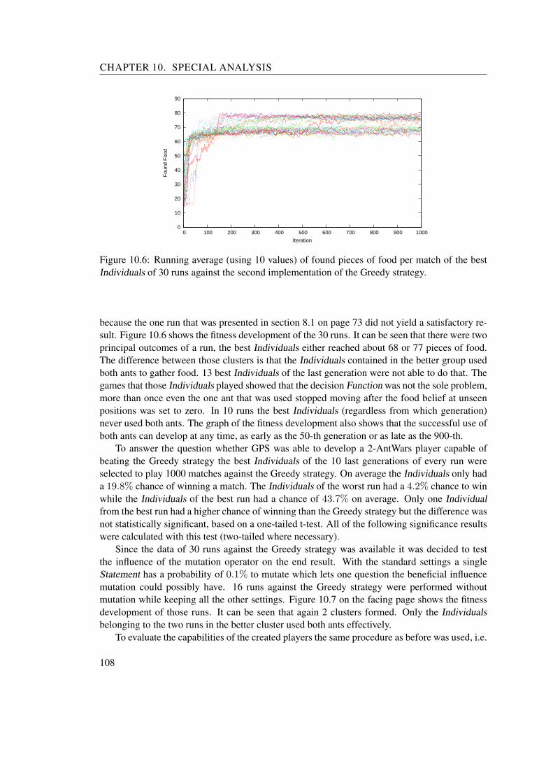
CHAPTER 10. SPECIAL ANALYSIS
0
10
20
30
40
50
60
70
80
90
0 100 200 300 400 500 600 700 800 900 1000
Fou
nd F
ood
Iteration
Figure 10.6: Running average (using 10 values) of found pieces of food per match of the bestIndividuals of 30 runs against the second implementation of the Greedy strategy.
because the one run that was presented in section 8.1 on page 73 did not yield a satisfactory re-sult. Figure 10.6 shows the fitness development of the 30 runs. It can be seen that there were twoprincipal outcomes of a run, the best Individuals either reached about 68 or 77 pieces of food.The difference between those clusters is that the Individuals contained in the better group usedboth ants to gather food. 13 best Individuals of the last generation were not able to do that. Thegames that those Individuals played showed that the decision Function was not the sole problem,more than once even the one ant that was used stopped moving after the food belief at unseenpositions was set to zero. In 10 runs the best Individuals (regardless from which generation)never used both ants. The graph of the fitness development also shows that the successful use ofboth ants can develop at any time, as early as the 50-th generation or as late as the 900-th.
To answer the question whether GPS was able to develop a 2-AntWars player capable ofbeating the Greedy strategy the best Individuals of the 10 last generations of every run wereselected to play 1000 matches against the Greedy strategy. On average the Individuals only hada 19.8% chance of winning a match. The Individuals of the worst run had a 4.2% chance to winwhile the Individuals of the best run had a chance of 43.7% on average. Only one Individualfrom the best run had a higher chance of winning than the Greedy strategy but the difference wasnot statistically significant, based on a one-tailed t-test. All of the following significance resultswere calculated with this test (two-tailed where necessary).
Since the data of 30 runs against the Greedy strategy was available it was decided to testthe influence of the mutation operator on the end result. With the standard settings a singleStatement has a probability of 0.1% to mutate which lets one question the beneficial influencemutation could possibly have. 16 runs against the Greedy strategy were performed withoutmutation while keeping all the other settings. Figure 10.7 on the facing page shows the fitnessdevelopment of those runs. It can be seen that again 2 clusters formed. Only the Individualsbelonging to the two runs in the better cluster used both ants effectively.
To evaluate the capabilities of the created players the same procedure as before was used, i.e.
108

10.3. PLAYING AGAINST UNKNOWN OPPONENTS
0
10
20
30
40
50
60
70
80
90
0 100 200 300 400 500 600 700 800 900 1000
Fou
nd F
ood
Iteration
Figure 10.7: Running average (using 10 values) of found pieces of food per match of the bestIndividuals of 16 runs without mutation against the second implementation of the Greedy strat-egy.
the best Individuals of the last 10 generations of every run had to play 1000 games against theGreedy strategy. On average, the Individuals had a 7.8% chance of winning, which is far worsethan the runs with enabled mutation. The difference is significant at the 1% level. This provesthat, at least when developing players against the second implementation of the Greedy strategy,runs using mutation yield far better results. The usefulness of the crossover operator was alreadyseen in the runs where beneficial movement behaviour switched between the movement1 andmovement2 Functions.
10.3 Playing against Unknown Opponents
While 2-AntWars players are developed, they are always battled against the same (or the threesame) fixed strategies or against players from the same generation in coevolutionary runs. It isexpected that the developed players adapt to their opponents to be able to beat them. The extentof the adaption, however, is unknown. For instance, are players that were developed against theScorched Earth strategy able to beat other strategies or is their behaviour only successful againstthis one strategy? A related question concerns the development of players in coevolutionaryruns. Is a player that is superior to its current opponent also able to beat opponents from previousgenerations? The expected answer is no, because coevolution does in no way ensure this; seethe discussion of historical progress in chapter 2 on page 5. With this kind of data available alsoa third question can be answered. Do the developed players use the position predictions of theenemy’s ants in a constructive way or do they ignore this information? In the analysis of the runsagainst fixed strategies it could not be observed that the position predictions have any influenceat all on the performance of the developed players.
To determine the performance of the developed players, the best Individuals of the 10 lastgenerations of a run were chosen to represent the result of the run. Each of these Individuals then
109
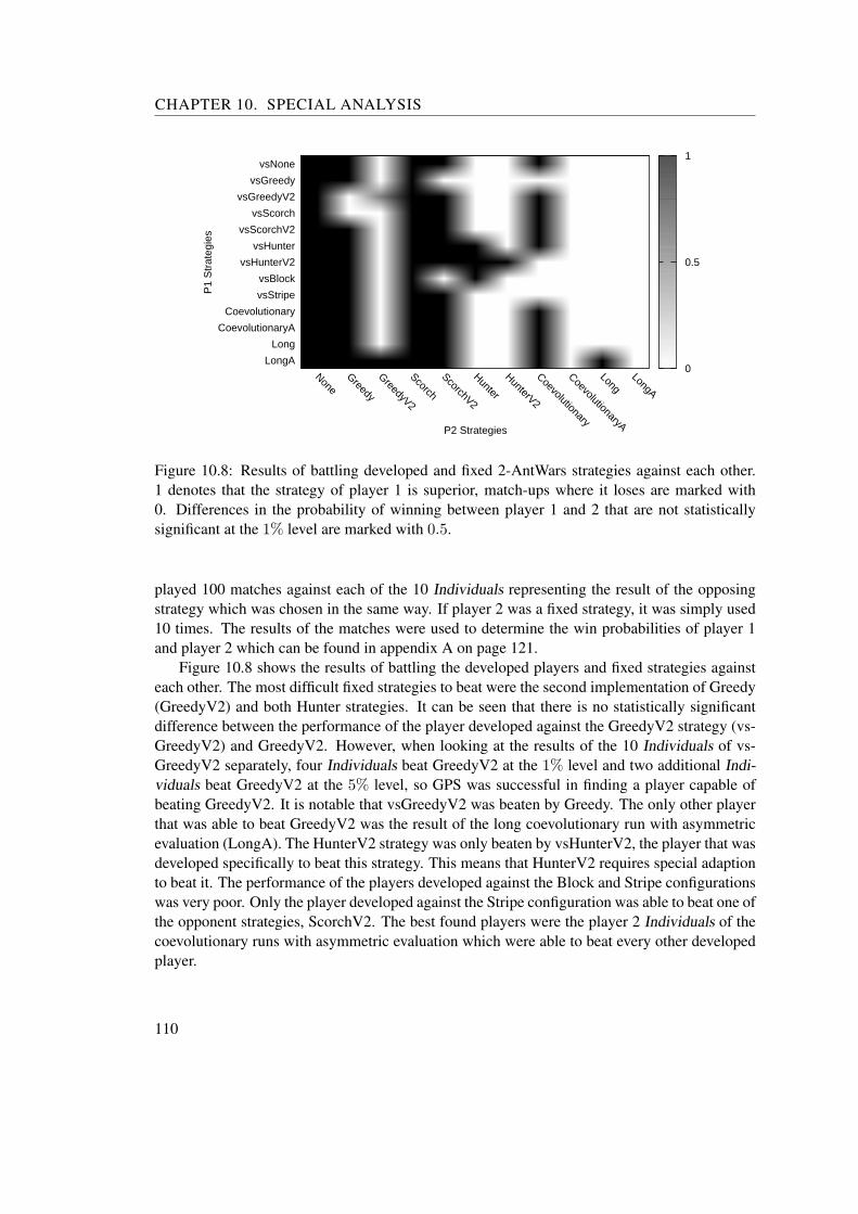
CHAPTER 10. SPECIAL ANALYSIS
vsNone
vsGreedy
vsGreedyV2
vsScorch
vsScorchV2
vsHunter
vsHunterV2
vsBlock
vsStripe
Coevolutionary
CoevolutionaryA
Long
LongANone
Greedy
GreedyV2
Scorch
ScorchV2
Hunter
HunterV2
Coevolutionary
CoevolutionaryA
LongLongA
P1
Str
ateg
ies
P2 Strategies
0
0.5
1
Figure 10.8: Results of battling developed and fixed 2-AntWars strategies against each other.1 denotes that the strategy of player 1 is superior, match-ups where it loses are marked with0. Differences in the probability of winning between player 1 and 2 that are not statisticallysignificant at the 1% level are marked with 0.5.
played 100 matches against each of the 10 Individuals representing the result of the opposingstrategy which was chosen in the same way. If player 2 was a fixed strategy, it was simply used10 times. The results of the matches were used to determine the win probabilities of player 1and player 2 which can be found in appendix A on page 121.
Figure 10.8 shows the results of battling the developed players and fixed strategies againsteach other. The most difficult fixed strategies to beat were the second implementation of Greedy(GreedyV2) and both Hunter strategies. It can be seen that there is no statistically significantdifference between the performance of the player developed against the GreedyV2 strategy (vs-GreedyV2) and GreedyV2. However, when looking at the results of the 10 Individuals of vs-GreedyV2 separately, four Individuals beat GreedyV2 at the 1% level and two additional Indi-viduals beat GreedyV2 at the 5% level, so GPS was successful in finding a player capable ofbeating GreedyV2. It is notable that vsGreedyV2 was beaten by Greedy. The only other playerthat was able to beat GreedyV2 was the result of the long coevolutionary run with asymmetricevaluation (LongA). The HunterV2 strategy was only beaten by vsHunterV2, the player that wasdeveloped specifically to beat this strategy. This means that HunterV2 requires special adaptionto beat it. The performance of the players developed against the Block and Stripe configurationswas very poor. Only the player developed against the Stripe configuration was able to beat one ofthe opponent strategies, ScorchV2. The best found players were the player 2 Individuals of thecoevolutionary runs with asymmetric evaluation which were able to beat every other developedplayer.
110
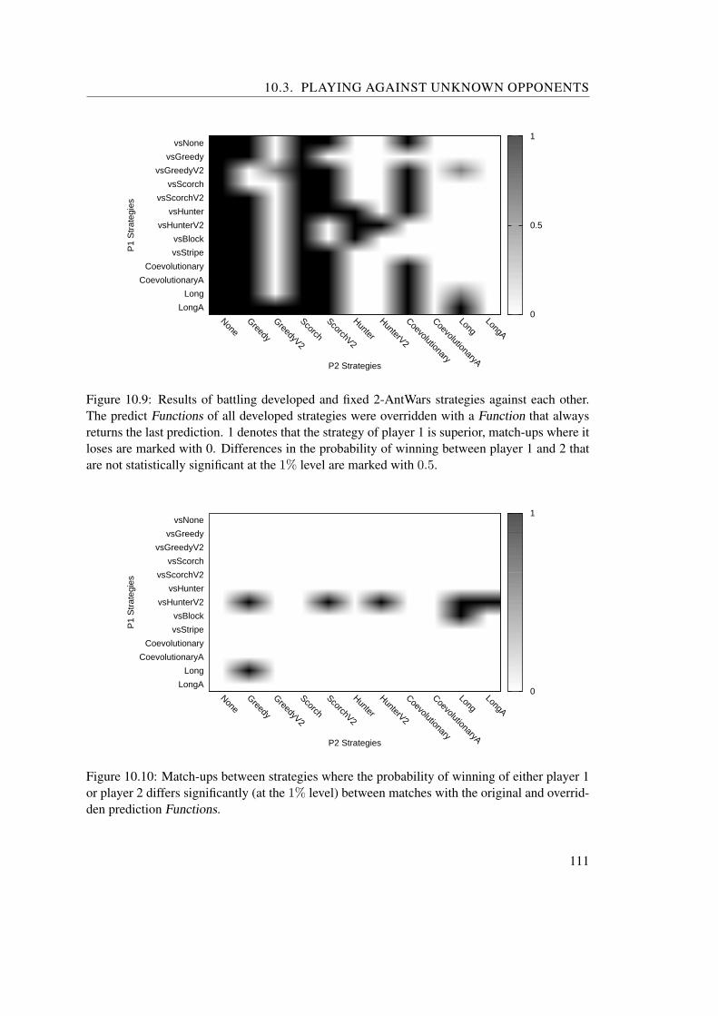
10.3. PLAYING AGAINST UNKNOWN OPPONENTS
vsNone
vsGreedy
vsGreedyV2
vsScorch
vsScorchV2
vsHunter
vsHunterV2
vsBlock
vsStripe
Coevolutionary
CoevolutionaryA
Long
LongANone
Greedy
GreedyV2
Scorch
ScorchV2
Hunter
HunterV2
Coevolutionary
CoevolutionaryA
LongLongA
P1
Str
ateg
ies
P2 Strategies
0
0.5
1
Figure 10.9: Results of battling developed and fixed 2-AntWars strategies against each other.The predict Functions of all developed strategies were overridden with a Function that alwaysreturns the last prediction. 1 denotes that the strategy of player 1 is superior, match-ups where itloses are marked with 0. Differences in the probability of winning between player 1 and 2 thatare not statistically significant at the 1% level are marked with 0.5.
vsNone
vsGreedy
vsGreedyV2
vsScorch
vsScorchV2
vsHunter
vsHunterV2
vsBlock
vsStripe
Coevolutionary
CoevolutionaryA
Long
LongANone
Greedy
GreedyV2
Scorch
ScorchV2
Hunter
HunterV2
Coevolutionary
CoevolutionaryA
LongLongA
P1
Str
ateg
ies
P2 Strategies
0
1
Figure 10.10: Match-ups between strategies where the probability of winning of either player 1or player 2 differs significantly (at the 1% level) between matches with the original and overrid-den prediction Functions.
111

CHAPTER 10. SPECIAL ANALYSIS
Figure 10.9 on the preceding page shows the same results after the prediction Functions ofthe developed players were overridden with a prediction Function that always returns the lastprediction, which is equivalent to the starting position or the location where the enemy’s ant waslast seen. The results are essentially the same, but in two additional match-ups the performancedifference is not statistically significant. This is a hint that the predict Functions indeed havean influence on the performance of the developed players. Figure 10.10 on the previous pageshows this more clearly. Especially the performance of vsHunterV2 is significantly influencedby changed predict Functions. Contrary to expectations the performance of vsHunterV2 actu-ally improved from a 52.7% to a 55.3% chance of winning a match against HunterV2. In theother two match-ups the player 1 strategy suffers a reduction in performance when the predictFunctions are overridden.
To evaluate the strategies developed during the long coevolutionary run, 10 Individuals werechosen from six distinct phases of the fitness development of this run that was shown in fig-ure 9.16 on page 101. No Individuals were chosen from the first 5000 generations becauseplayer 2 had not developed the use of both ants. Player 2 dominated at generations 5000 and5500, player 1 gained the upper hand at generation 6800. At generation 8000 both playersseemed to be on equal footing. Player 2 won around generation 9500 and player 1 at the end ofthe run. The Individuals of each phase were chosen among the best Individuals from generationsaround the mentioned ones. Only Individuals were chosen that conformed to the current trend,for instance for generation 5000, players from a particular generation (around generation 5000)were only chosen if player 2 beat player 1. For the phase around generation 8000 five generations
5000
5500
6800
8000
9500
9999
5000 5500 6800 8000 9500 9999
P1
Str
ateg
ies
P2 Strategies
0
0.5
1
Figure 10.11: Results of battling Individuals from different generations of the long coevolution-ary run against each other. 1 denotes that the strategy of player 1 is superior, match-ups where itloses are marked with 0. Differences in the probability of winning between player 1 and 2 thatare not statistically significant at the 1% level are marked with 0.5.
112
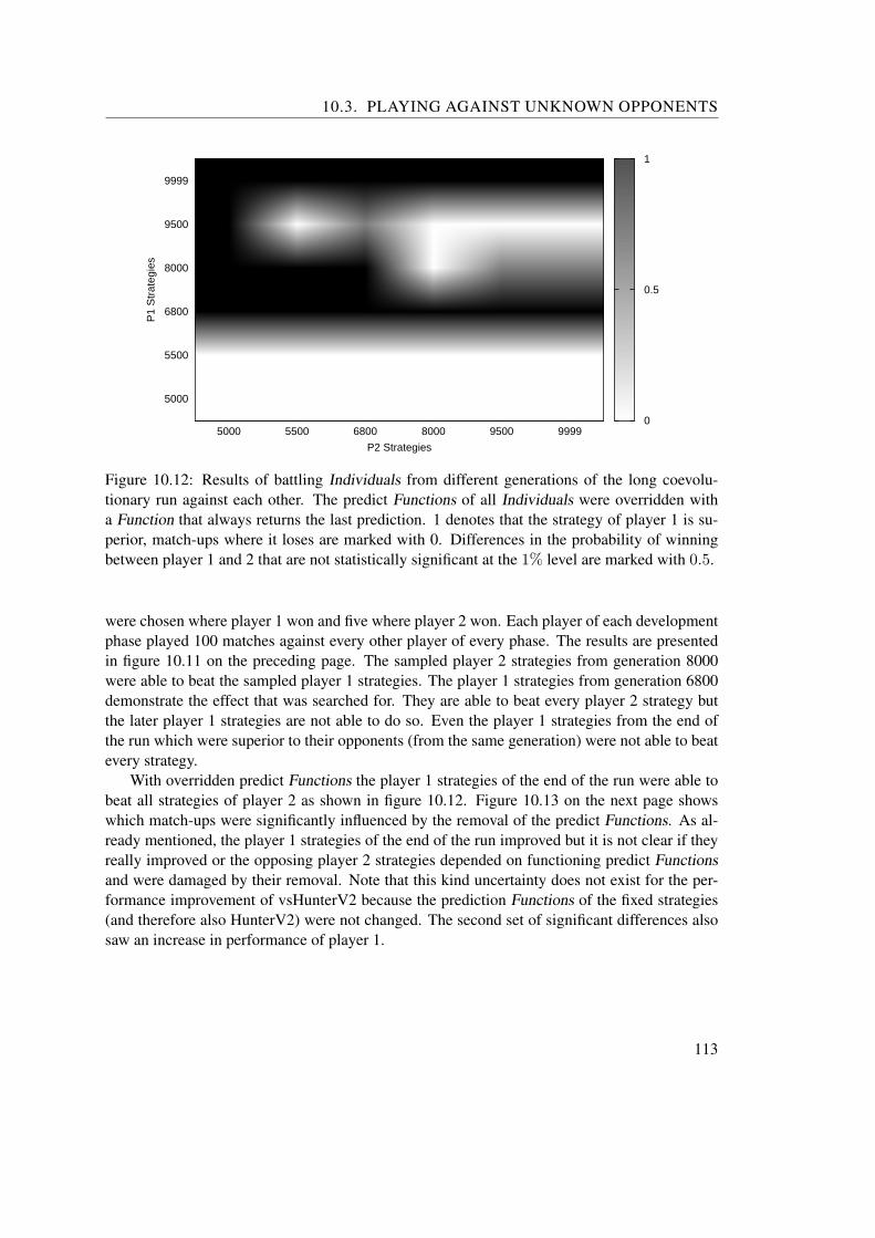
10.3. PLAYING AGAINST UNKNOWN OPPONENTS
5000
5500
6800
8000
9500
9999
5000 5500 6800 8000 9500 9999
P1
Str
ateg
ies
P2 Strategies
0
0.5
1
Figure 10.12: Results of battling Individuals from different generations of the long coevolu-tionary run against each other. The predict Functions of all Individuals were overridden witha Function that always returns the last prediction. 1 denotes that the strategy of player 1 is su-perior, match-ups where it loses are marked with 0. Differences in the probability of winningbetween player 1 and 2 that are not statistically significant at the 1% level are marked with 0.5.
were chosen where player 1 won and five where player 2 won. Each player of each developmentphase played 100 matches against every other player of every phase. The results are presentedin figure 10.11 on the preceding page. The sampled player 2 strategies from generation 8000were able to beat the sampled player 1 strategies. The player 1 strategies from generation 6800demonstrate the effect that was searched for. They are able to beat every player 2 strategy butthe later player 1 strategies are not able to do so. Even the player 1 strategies from the end ofthe run which were superior to their opponents (from the same generation) were not able to beatevery strategy.
With overridden predict Functions the player 1 strategies of the end of the run were able tobeat all strategies of player 2 as shown in figure 10.12. Figure 10.13 on the next page showswhich match-ups were significantly influenced by the removal of the predict Functions. As al-ready mentioned, the player 1 strategies of the end of the run improved but it is not clear if theyreally improved or the opposing player 2 strategies depended on functioning predict Functionsand were damaged by their removal. Note that this kind uncertainty does not exist for the per-formance improvement of vsHunterV2 because the prediction Functions of the fixed strategies(and therefore also HunterV2) were not changed. The second set of significant differences alsosaw an increase in performance of player 1.
113

CHAPTER 10. SPECIAL ANALYSIS
5000
5500
6800
8000
9500
9999
5000 5500 6800 8000 9500 9999
P1
Str
ateg
ies
P2 Strategies
0
1
Figure 10.13: Match-ups between strategies extracted from the long coevolutionary run wherethe probability of winning of either player 1 or player 2 differs significantly (at the 1% level)between matches with the original and overridden prediction Functions.
114
CHAPTER 11Conclusion
In the course of this thesis, the results of nine evolutionary and four coevolutionary experimentsto develop capable 2-AntWars players were presented. It was demonstrated that the used geneticprogramming system was powerful enough to beat all of the seven static game strategies.
The basis of all developed players was greedy movement in order to to collect as muchfood as possible, but the details varied a lot and were tailored to the specific strategy of theopponent. The first implementation of the Scorched Earth strategy for example was beaten byReverse Scorched Earth; the developed player moved one of his ants into the opponent’s halfof the playing field and collected the food located there before the opponent (playing ScorchedEarth) had the opportunity. This strategy even reduced the greediness of one ant to get it fasterinto the opponent’s half. The two implementations of the Hunter strategy were beaten by baitingthe, and hiding from the, hunting ant respectively. In addition, the battle support mechanic wasused to combat the hunting ant. During most of the runs the developed players showed a ratherpacifistic behaviour by ignoring the opposing ants. One exception, however, was the run againstthe second implementation of the Greedy strategy, the developed player routinely neutralizedone of the opponent’s ants.
Another trend that was observed during the runs was that the developed players always usedone ant until it was not able to move anymore before the second ant was moved. Which antmoved first depended on the opponent. For instance, against the first implementation of theHunter strategy ant 1 was moved first, against the second implementation of the Greedy strategyant 2 was dominant. When faced with the second implementation of the Hunter strategy, usinga specific ant first did not yield any advantage and the population was split in two halves, onemoving ant 1 first and one ant 2. Of course there were exceptions to this general trend. Innearly every run species emerged that switched the moved ant more freely, but those speciesdid not survive unless it was a clear advantage. This was the case in the run against the secondimplementation of the Hunter strategy, where both ants were moved early to hide from thehunting ant of the opponent. Repeated runs against the second implementation of the Greedystrategy showed that about 1/3 of the conducted runs did not create players that are able to useboth ants effectively.
115
CHAPTER 11. CONCLUSION
The success of the runs was not only due to high performing movement and decision Func-tions. The belief Functions in particular developed some interesting methods of approximatingthe disappearance of food from the playing field. Most of them were based on switching thefood belief from one to zero instead of interpolating between those values based on the elapsedtime. The interpolation of belief only occurred in the run against the first implementation of theGreedy strategy. During all other runs the developed belief Function started out with food beliefeverywhere and then switched it off based on time. This switch-off occurred in multiple variantsdepending on the opponent that was faced. Sometimes the food belief for all unseen fields wasset to zero and sometimes the disbelief grew row wise or column wise from the starting positionsof the opponent’s ants and once the disbelief grew row wise from the top of the playing field tothe bottom. The behaviour of the belief Function was observed to have significant influenceon the performance of the player. Unfortunately, this influence was not always positive, in atleast three runs otherwise superior species went extinct or suffered a significant performancepenalty because they were depending on a non-optimal belief Function. In the run against thesecond implementation of the Scorched Earth strategy a species was able to adapt to a changedbehaviour of the belief Function and regained its lost performance.
The contribution of the predict Functions to the overall performance of players was ques-tionable. Overriding the developed Functions either did not change the fitness in a significantway or actually improved it. Two principal behaviours were observed with the predict Functions,jumping with the prediction to some location that is a reasonable approximation of the positionof the predicted ant or moving the prediction from the starting position to such a location.
The coevolutionary runs showed that it is possible for the players to adapt to each other ina way that one species in one population beats the Individuals at their positions in the otherpopulation while the other population contains a second species that beats Individuals in thefirst population at their positions. The experiments testing long term coevolution demonstratedthat the populations were not subject to loss of gradient or disengagement. They battled fiercelyfor dominance and the inferior player always developed a way to gain the upper hand again.Historical progress could not be observed as the players of later generations in some cases lostto players from earlier generations. Asymmetric evaluation did not yield any notable changes inthe evolutionary process besides taking three times longer than symmetric evaluation.
The deeper analysis of the runs unearthed some quite interesting evolutionary behaviour.The first coevolutionary run showed that movement capabilities of one movement Function canswitch almost seamlessly to the movement Function of the other ant. The same run also demon-strated that the combination of two species can yield a new species that is superior to both whena species with an exceptional movement Function for one ant combined with a species that usedboth ants to collect food. This proves the usefulness of the crossover operator for the 2-AntWarsproblem. Mutation was also instrumental for the success of the runs as removing mutation in-creased the chance of not discovering the use of both ants from 1/3 to 7/8. In the first run withasymmetric evaluation there were two species in a row that reduced the amount of positions theyuncovered to improve their performance, which is quite counter-intuitive because normally moreuncovered fields result in more opportunities to find food. In these cases not exploring every po-sition was advantageous because the unexplored positions were most likely already harvestedby the enemy’s ants and so the available moves could be spent more wisely.
116

Generally, the populations converged to one level of fitness but that does not mean that therewas a loss of diversity. Often there were species contained in the populations that chose differentants for the majority of the game, moved less random than others or were more aggressive,so after a run had finished there were lots of Individuals with different successful strategiesavailable. This was especially true of the long coevolutionary runs where both parts of thepopulations developed capable players and only small variances in playing style tipped the scalesfrom one player to the other.
From the point of view of evaluating the rules of 2-AntWars, it seemed that there are notenough reasons to use both ants simultaneously. In some runs this simultaneous use emergedonly to die out again. With the rules as they are now, a game is split up into two phases. In thefirst phase one ant of each player tries to find as much food as possible and in the second phasethe other ant of each player tries to find the food that was left behind. When two competentplayers face each other, the second phase is usually short, with the ants finding about 2 piecesof food on average. Maybe it would have been a good idea to reduce the allowed moves by theants. That way a movable ant is more valuable and both ants of both players are really neededto find all the food on the playing field.
There are multiple directions for future research. One main task is to make it feasible torepeat runs multiple times to investigate the influence the population model and selection op-erator have on the final result. This thesis demonstrated that the chosen model and selectionoperator enabled the creation of multiple species inside the population but it is not clear that thishas a positive influence on the final outcome. The chosen selection operator could probably beimproved by taking the stochastic nature of evaluation into account, for instance it could use astatistic test to determine if one Individual is significantly better than another one. Furthermore,it could be beneficial to develop a system that automatically recognises an emerging species andputs it into a repository, so that one long coevolutionary run is enough to create a wide rangeof successful playing strategies without human intervention. Another direction for research isadapting the rules of 2-AntWars to explore the influence of changed rules on the playing styleof the developed players. Reducing the number of allowed moves per ant was already men-tioned, other possibilities are adding a third ant for each player, making the capabilities of theants asymmetric (e.g. one ant can move faster but the other ant sees further) or reducing thenumber of games per match to see when the noise of random food placement prevents evolu-tionary progress. A third direction could be adapting the model of the 2-AntWars player. It wasalready seen that the predict Functions did not help the performance of the players but more fun-damental changes could also result in a more capable playing style. The presented model wasdecision based, i.e. Functions calculated explicitly the next move. Another possibility would beto develop scoring functions for each possible move and the move with the highest score will beexecuted.
117


Part IV
Appendix

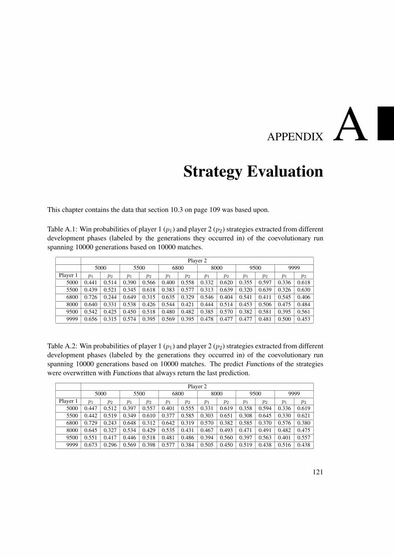
APPENDIX AStrategy Evaluation
This chapter contains the data that section 10.3 on page 109 was based upon.
Table A.1: Win probabilities of player 1 (p1) and player 2 (p2) strategies extracted from differentdevelopment phases (labeled by the generations they occurred in) of the coevolutionary runspanning 10000 generations based on 10000 matches.
Player 25000 5500 6800 8000 9500 9999
Player 1 p1 p2 p1 p2 p1 p2 p1 p2 p1 p2 p1 p2
5000 0.441 0.514 0.390 0.566 0.400 0.558 0.332 0.620 0.355 0.597 0.336 0.6185500 0.439 0.521 0.345 0.618 0.383 0.577 0.313 0.639 0.320 0.639 0.326 0.6306800 0.726 0.244 0.649 0.315 0.635 0.329 0.546 0.404 0.541 0.411 0.545 0.4068000 0.640 0.331 0.538 0.426 0.544 0.421 0.444 0.514 0.453 0.506 0.475 0.4849500 0.542 0.425 0.450 0.518 0.480 0.482 0.385 0.570 0.382 0.581 0.395 0.5619999 0.656 0.315 0.574 0.395 0.569 0.395 0.478 0.477 0.477 0.481 0.500 0.453
Table A.2: Win probabilities of player 1 (p1) and player 2 (p2) strategies extracted from differentdevelopment phases (labeled by the generations they occurred in) of the coevolutionary runspanning 10000 generations based on 10000 matches. The predict Functions of the strategieswere overwritten with Functions that always return the last prediction.
Player 25000 5500 6800 8000 9500 9999
Player 1 p1 p2 p1 p2 p1 p2 p1 p2 p1 p2 p1 p2
5000 0.447 0.512 0.397 0.557 0.401 0.555 0.331 0.619 0.358 0.594 0.336 0.6195500 0.442 0.519 0.349 0.610 0.377 0.585 0.303 0.651 0.308 0.645 0.330 0.6216800 0.729 0.243 0.648 0.312 0.642 0.319 0.570 0.382 0.585 0.370 0.576 0.3808000 0.645 0.327 0.534 0.429 0.535 0.431 0.467 0.493 0.471 0.491 0.482 0.4759500 0.551 0.417 0.446 0.518 0.481 0.486 0.394 0.560 0.397 0.563 0.401 0.5579999 0.673 0.296 0.569 0.398 0.577 0.384 0.505 0.450 0.519 0.438 0.516 0.438
121
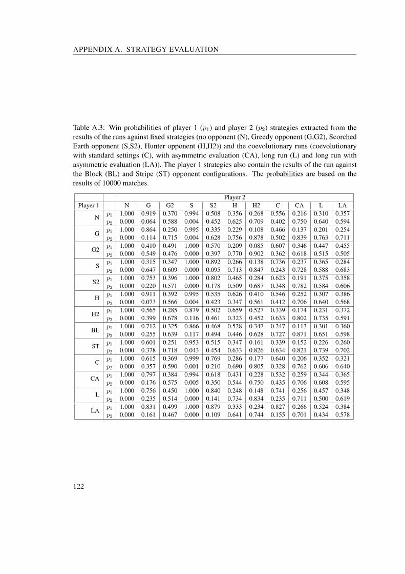
APPENDIX A. STRATEGY EVALUATION
Table A.3: Win probabilities of player 1 (p1) and player 2 (p2) strategies extracted from theresults of the runs against fixed strategies (no opponent (N), Greedy opponent (G,G2), ScorchedEarth opponent (S,S2), Hunter opponent (H,H2)) and the coevolutionary runs (coevolutionarywith standard settings (C), with asymmetric evaluation (CA), long run (L) and long run withasymmetric evaluation (LA)). The player 1 strategies also contain the results of the run againstthe Block (BL) and Stripe (ST) opponent configurations. The probabilities are based on theresults of 10000 matches.
Player 2Player 1 N G G2 S S2 H H2 C CA L LA
Np1 1.000 0.919 0.370 0.994 0.508 0.356 0.268 0.556 0.216 0.310 0.357p2 0.000 0.064 0.588 0.004 0.452 0.625 0.709 0.402 0.750 0.640 0.594
Gp1 1.000 0.864 0.250 0.995 0.335 0.229 0.108 0.466 0.137 0.201 0.254p2 0.000 0.114 0.715 0.004 0.628 0.756 0.878 0.502 0.839 0.763 0.711
G2p1 1.000 0.410 0.491 1.000 0.570 0.209 0.085 0.607 0.346 0.447 0.455p2 0.000 0.549 0.476 0.000 0.397 0.770 0.902 0.362 0.618 0.515 0.505
Sp1 1.000 0.315 0.347 1.000 0.892 0.266 0.138 0.736 0.237 0.365 0.284p2 0.000 0.647 0.609 0.000 0.095 0.713 0.847 0.243 0.728 0.588 0.683
S2p1 1.000 0.753 0.396 1.000 0.802 0.465 0.284 0.623 0.191 0.375 0.358p2 0.000 0.220 0.571 0.000 0.178 0.509 0.687 0.348 0.782 0.584 0.606
Hp1 1.000 0.911 0.392 0.995 0.535 0.626 0.410 0.546 0.252 0.307 0.386p2 0.000 0.073 0.566 0.004 0.423 0.347 0.561 0.412 0.706 0.640 0.568
H2p1 1.000 0.565 0.285 0.879 0.502 0.659 0.527 0.339 0.174 0.231 0.372p2 0.000 0.399 0.678 0.116 0.461 0.323 0.452 0.633 0.802 0.735 0.591
BLp1 1.000 0.712 0.325 0.866 0.468 0.528 0.347 0.247 0.113 0.301 0.360p2 0.000 0.255 0.639 0.117 0.494 0.446 0.628 0.727 0.871 0.651 0.598
STp1 1.000 0.601 0.251 0.953 0.515 0.347 0.161 0.339 0.152 0.226 0.260p2 0.000 0.378 0.718 0.043 0.454 0.633 0.826 0.634 0.821 0.739 0.702
Cp1 1.000 0.615 0.369 0.999 0.769 0.286 0.177 0.640 0.206 0.352 0.321p2 0.000 0.357 0.590 0.001 0.210 0.690 0.805 0.328 0.762 0.606 0.640
CAp1 1.000 0.797 0.384 0.994 0.618 0.431 0.228 0.532 0.259 0.344 0.365p2 0.000 0.176 0.575 0.005 0.350 0.544 0.750 0.435 0.706 0.608 0.595
Lp1 1.000 0.756 0.450 1.000 0.840 0.248 0.148 0.741 0.256 0.457 0.348p2 0.000 0.235 0.514 0.000 0.141 0.734 0.834 0.235 0.711 0.500 0.619
LAp1 1.000 0.831 0.499 1.000 0.879 0.333 0.234 0.827 0.266 0.524 0.384p2 0.000 0.161 0.467 0.000 0.109 0.641 0.744 0.155 0.701 0.434 0.578
122

Table A.4: Win probabilities of player 1 (p1) and player 2 (p2) strategies extracted from theresults of the runs against fixed strategies (no opponent (N), Greedy opponent (G,G2), ScorchedEarth opponent (S,S2), Hunter opponent (H,H2)) and the coevolutionary runs (coevolutionarywith standard settings (C), with asymmetric evaluation (CA), long run (L) and long run withasymmetric evaluation (LA). The player 1 strategies also contain the results of the run againstthe Block (BL) and Stripe (ST) opponent configurations. The predict Functions of the player 1and the coevolutionary player 2 strategies were overwritten with a Function that always returnsthe last prediction. The probabilities are based on the results of 10000 matches.
Player 2Player 1 N G G2 S S2 H H2 C CA L LA
Np1 1.000 0.921 0.363 0.994 0.518 0.368 0.276 0.555 0.211 0.293 0.366p2 0.000 0.062 0.597 0.004 0.443 0.613 0.702 0.405 0.759 0.656 0.591
Gp1 1.000 0.856 0.243 0.997 0.334 0.230 0.111 0.460 0.136 0.189 0.241p2 0.000 0.120 0.725 0.002 0.633 0.752 0.875 0.506 0.842 0.777 0.726
G2p1 1.000 0.423 0.488 1.000 0.566 0.203 0.078 0.606 0.347 0.470 0.455p2 0.000 0.533 0.478 0.000 0.395 0.783 0.914 0.358 0.620 0.490 0.508
Sp1 1.000 0.305 0.345 1.000 0.887 0.264 0.138 0.723 0.231 0.378 0.278p2 0.000 0.656 0.612 0.000 0.100 0.712 0.846 0.255 0.736 0.577 0.688
S2p1 1.000 0.758 0.388 1.000 0.798 0.457 0.291 0.619 0.187 0.380 0.352p2 0.000 0.217 0.576 0.000 0.181 0.518 0.685 0.352 0.784 0.579 0.608
Hp1 1.000 0.911 0.387 0.996 0.538 0.639 0.409 0.542 0.254 0.283 0.386p2 0.000 0.074 0.566 0.003 0.421 0.339 0.564 0.411 0.709 0.666 0.566
H2p1 1.000 0.606 0.301 0.877 0.412 0.676 0.553 0.345 0.180 0.194 0.402p2 0.000 0.354 0.661 0.116 0.552 0.308 0.423 0.625 0.800 0.767 0.557
BLp1 1.000 0.710 0.332 0.863 0.463 0.530 0.347 0.252 0.108 0.259 0.359p2 0.000 0.257 0.631 0.122 0.501 0.442 0.627 0.723 0.873 0.695 0.597
STp1 1.000 0.604 0.248 0.952 0.520 0.343 0.164 0.330 0.152 0.214 0.257p2 0.000 0.372 0.721 0.043 0.450 0.636 0.819 0.640 0.825 0.755 0.708
Cp1 1.000 0.620 0.368 0.999 0.762 0.285 0.172 0.640 0.206 0.350 0.324p2 0.000 0.351 0.593 0.001 0.217 0.691 0.812 0.331 0.760 0.610 0.638
CAp1 1.000 0.800 0.400 0.995 0.617 0.432 0.232 0.523 0.258 0.336 0.364p2 0.000 0.175 0.562 0.004 0.351 0.545 0.748 0.439 0.706 0.623 0.594
Lp1 1.000 0.707 0.440 1.000 0.842 0.244 0.146 0.736 0.248 0.470 0.344p2 0.000 0.278 0.523 0.000 0.142 0.735 0.836 0.240 0.720 0.488 0.618
LAp1 1.000 0.833 0.501 1.000 0.882 0.340 0.241 0.822 0.265 0.537 0.389p2 0.000 0.159 0.465 0.000 0.106 0.632 0.737 0.159 0.701 0.423 0.582
123


Bibliography
[1] Antwars competition, April 2010. http://www.sigevo.org/gecco-2007/competitions.html#c3.
[2] Christoph Salge, Christian Lipski, Tobias Mahlmann, and Brigitte Mathiak. Using genet-ically optimized artificial intelligence to improve gameplaying fun for strategical games.In Sandbox ’08: Proceedings of the 2008 ACM SIGGRAPH symposium on Video games,pages 7–14, New York, NY, USA, 2008. ACM.
[3] John R. Koza. Genetic Programming: On the Programming of Computers by Means ofNatural Selection (Complex Adaptive Systems). The MIT Press, December 1992.
[4] Tiago Francisco and Gustavo Miguel Jorge dos Reis. Evolving combat algorithms to con-trol space ships in a 2d space simulation game with co-evolution using genetic program-ming and decision trees. In GECCO ’08: Proceedings of the 2008 GECCO conferencecompanion on Genetic and evolutionary computation, pages 1887–1892, New York, NY,USA, 2008. ACM.
[5] Tiago Francisco and Gustavo Miguel Jorge dos Reis. Evolving predator and prey be-haviours with co-evolution using genetic programming and decision trees. In GECCO’08: Proceedings of the 2008 GECCO conference companion on Genetic and evolutionarycomputation, pages 1893–1900, New York, NY, USA, 2008. ACM.
[6] Sean Luke and Lee Spector. Evolving teamwork and coordination with genetic program-ming. In John R. Koza, David E. Goldberg, David B. Fogel, and Rick L. Riolo, editors,Genetic Programming 1996: Proceedings of the First Annual Conference, pages 150–156,Stanford University, CA, USA, 28–31 July 1996. MIT Press.
[7] Sean Luke, Charles Hohn, Jonathan Farris, Gary Jackson, and James Hendler. Co-evolvingsoccer softbot team coordination with genetic programming. In Hiroaki Kitano, editor,RoboCup-97: Robot Soccer World Cup I, volume 1395 of Lecture Notes in ComputerScience, pages 398–411. Springer-Verlag, 1997.
[8] Ami Hauptman. Gp-endchess: Using genetic programming to evolve chess endgameplayers. In Maarten Keijzer, Andrea Tettamanzi, Pierre Collet, Jano van Hemert, andMarco Tomassini, editors, Proceedings of 8th European Conference on Genetic Program-ming (EuroGP2005), volume 3447 of Lecture Notes in Computer Science, pages 120–131.Springer, 2005.
125

BIBLIOGRAPHY
[9] Timothy Perkis. Stack-based genetic programming. In Proceedings of the 1994 IEEEWorld Congress on Computational Intelligence, volume 1, pages 148–153, Orlando,Florida, USA, 27-29 June 1994. IEEE Press.
[10] Markus F. Brameier and Wolfgang Banzhaf. Linear Genetic Programming (Genetic andEvolutionary Computation). Springer-Verlag New York, Inc., Secaucus, NJ, USA, 2006.
[11] Julian F. Miller and Peter Thomson. Cartesian genetic programming. In RiccardoPoli, Wolfgang Banzhaf, William B. Langdon, Julian F. Miller, Peter Nordin, and Ter-ence C. Fogarty, editors, Genetic Programming, Proceedings of EuroGP’2000, volume1802 of Lecture Notes in Computer Science, pages 121–132, Edinburgh, 15-16 April 2000.Springer-Verlag.
[12] Riccardo Poli. Parallel distributed genetic programming. In David Corne, Marco Dorigo,Fred Glover, Dipankar Dasgupta, Pablo Moscato, Riccardo Poli, and Kenneth V. Price,editors, New ideas in optimization, pages 403–432. McGraw-Hill Ltd., UK, Maidenhead,UK, England, 1999.
[13] Peter A. Whigham. Grammatically-based genetic programming. In Justinian P. Rosca,editor, Proceedings of the Workshop on Genetic Programming: From Theory to Real-WorldApplications, pages 33–41, Tahoe City, California, USA, 9 July 1995.
[14] David J. Montana. Strongly typed genetic programming. Evolutionary Computation,3:199–230, 1994.
[15] John R. Woodward and Ruibin Bai. Why evolution is not a good paradigm for programinduction: a critique of genetic programming. In GEC ’09: Proceedings of the firstACM/SIGEVO Summit on Genetic and Evolutionary Computation, pages 593–600, NewYork, NY, USA, 2009. ACM.
[16] Lorenz Huelsbergen. Finding general solutions to the parity problem by evolving machine-language representations. In Morgan Kaufmann, editor, Genetic Programming 1998: Pro-ceedings of the Third Annual Conference, pages 158–166. University of Wisconsin, Madi-son, Wisconsin, USA, July 1998.
[17] Sean Luke and Liviu Panait. A comparison of bloat control methods for genetic program-ming. Evol. Comput., 14(3):309–344, 2006.
[18] Sara Silva and Ernesto Costa. Dynamic limits for bloat control in genetic programming anda review of past and current bloat theories. Genetic Programming and Evolvable Machines,10(2):141–179, 2009.
[19] Daniel W. Hillis. Co-evolving parasites improve simulated evolution as an optimizationprocedure. Physica D: Nonlinear Phenomena, 42(1-3):228 – 234, 1990.
[20] Mitchell A. Potter and Kenneth A. de Jong. A cooperative coevolutionary approach tofunction optimization. In PPSN III: Proceedings of the International Conference on Evo-lutionary Computation. The Third Conference on Parallel Problem Solving from Nature,
126

volume 866 of Lecture Notes in Computer Science, pages 249–257, London, UK, 1994.Springer-Verlag.
[21] Peter J. Angeline and Jordan B. Pollack. Competitive environments evolve better solutionsfor complex tasks. In Stephanie Forrest, editor, Proceedings of the 5th International Con-ference on Genetic Algorithms, ICGA-93, pages 264–270, University of Illinois at Urbana-Champaign, 17-21 July 1993. Morgan Kaufmann.
[22] Thomas Miconi. Why coevolution doesn’t "work": Superiority and progress in coevolu-tion. In Leonardo Vanneschi, Steven Gustafson, Alberto Moraglio, Ivanoe De Falco, andMarc Ebner, editors, EuroGP, volume 5481 of Lecture Notes in Computer Science, pages49–60. Springer, 2009.
[23] Edwin D. de Jong, Kenneth O. Stanley, and R. Paul Wiegand. Introductory tutorial oncoevolution. In GECCO ’07: Proceedings of the 2007 GECCO conference companionon Genetic and evolutionary computation, pages 3133–3157, New York, NY, USA, 2007.ACM.
[24] John Nash. Non-cooperative games. The Annals of Mathematics, 54(2):286–295, Septem-ber 1951.
[25] Sevan G. Ficici and Anthony Bucci. Advanced tutorial on coevolution. In GECCO ’07:Proceedings of the 2007 GECCO conference companion on Genetic and evolutionary com-putation, pages 3172–3204, New York, NY, USA, 2007. ACM.
[26] Christopher D. Rosin and Richard K. Belew. New methods for competitive coevolution.Evolutionary Computation, 5(1):1–29, 1997.
[27] Kenneth O. Stanley and Risto Miikkulainen. The dominance tournament method of mon-itoring progress in coevolution. In Alwyn M. Barry, editor, GECCO 2002: Proceedingsof the Bird of a Feather Workshops, Genetic and Evolutionary Computation Conference,pages 242–248, New York, 8 July 2002. AAAI.
[28] Sevan G. Ficici and Jordan B. Pollack. A game-theoretic memory mechanism for co-evolution. In GECCO’03: Proceedings of the 2003 international conference on Geneticand evolutionary computation, volume 2723 of Lecture Notes in Computer Science, pages286–297, Berlin, Heidelberg, 2003. Springer-Verlag.
[29] Edwin D. de Jong. The incremental pareto-coevolution archive. In Proceedings of theGenetic and Evolutionary Computation Conference, GECCO04, volume 3102 of LectureNotes in Computer Science, pages 525–536. Springer Verlag, 2004.
[30] Nathan Williams and Melanie Mitchell. Investigating the success of spatial coevolution.In GECCO ’05: Proceedings of the 2005 conference on Genetic and evolutionary compu-tation, pages 523–530, New York, NY, USA, 2005. ACM.
[31] Mike J. Keith and Martin C. Martin. Genetic programming in c++: implementation issues.Advances in genetic programming, pages 285–310, 1994.
127

BIBLIOGRAPHY
[32] Wojciech Jaskowski, Krzysztof Krawiec, and Bartosz Wieloch. Winning ant wars: Evolv-ing a human-competitive game strategy using fitnessless selection. In Michael O’Neill,Leonardo Vanneschi, Steven Gustafson, Anna Esparcia-Alcázar, Ivanoe De Falco, Anto-nio Della Cioppa, and Ernesto Tarantino, editors, EuroGP, volume 4971 of Lecture Notesin Computer Science, pages 13–24. Springer, 2008.
128


![mitmachen[youknowit]helikon-online.de Hannes Liebrandt (2014): Napoleon I. und sein kontroverses Verhältnis zur Religion. Versuch einer historischen Einordnung. Geschichte, Gesellschaft](https://img.pdfslide.us/doc/110x75/60cc88940d18d66bca7fcc44/mitmachenyouknowithelikon-onlinede-hannes-liebrandt-2014-napoleon-i-und-sein.jpg)