Audio Engineering Society convention Pa per 5736users.spa.aalto.fi/mak/PUB/AES114_Hirvonen.pdf · Audio Engineering Society convention Pa per 5736 I ... (AMR) 12.2 kbit/s ... ity

HIKV U l W l M El' Ah.

Audio Engineering Society

convention Pa per 5736 I

Presented at the 114th Convention @ 2003 March 22-25 Amsterdam, The Netherlands

This convention paper has been reproduced from the author's advance manuscript, without editing, corrections, or consideration by the Review Board. The A E S takes n o responsibility for the contents. Additional papers m a y be obtained by sending request and remittance t o Audio Engineering Society, 60 East @nd Street, New York, New York 10165-2520, USA; also see www. aes. org. All rights reserved. Reproduction of this paper, or any portion thereof, is not permitted without direct permission from the Journal of the Audio Engineering Society.

Listening Test Methodology for Headphone Evaluation Toni Hirvonenl, Markus Vaalgamaa2, Juha Backman3, Matti Karjalainenl

Helsinki University of Technology, Lab. of Acoustics and Audio Signal Processing, P.O. Box 3000,FIN 02015 Espoo, Finland

Nokia Mobile Phones, Itamerenkatu 11 - 13, P.O. Box 407, FIN 00180 HELSINKI, Finland

Nokia Mobile Phones, Keilalahdentie 2 - 4, P.O. Box 100, FIN 02150 ESPOO, Finland

Correspondence should be addressed to Toni Hirvonen (toni@acoustics. hut. f i)

ABSTRACT Two listening tests with six different headphones were conducted using speech material. The objectives of these tests were to investigate listener sound color preferences using 1) the actual headphones and 2) dummy head recordings made with the same devices. The purpose of the recordings was to simulate the timbres of the actual devices as well as possible when played back through a pair of compensated headphones. The results from the two tests were compared and despite of some similarity, the analysis showed significant differences between the two cases. Additionally, the diffuse-field responses of the headphones were calculated from frequency response measurements. The obtained headphone preference order cannot fully be explained based on the flatness of the diffuse-field response as a measure.

AES 1 1 4 ~ ~ CONVENTION, AMSTERDAM, THE NETHERLANDS, 2003 MARCH 22-25

1 INTRODUCTION to the actual listening situation.

The initial motivation for the present investigation was to examine the quality and usefulness of artificial head recordings when evaluating the subjective quality of audio and telecommunication devices. An attempt was made to simulate the real-life sound sources used in listening tests by recording these same sources with a Head And Torso Simulator (HATS) and using one pair of compensated headphones as a reproduction device. These simulations were then compared to the real-life situation with the original devices. The audio devices used in these listening tests were chosen to be six different com- mercially available headphone models.

If this kind of simulation could be used, the listening test arrangements would be greatly simplified. The test arranger could theoretically replace com- plex test setups using for example a computer with a sound card and a pair of high-quality headphones. Different audio devices could be represented with recorded sound samples. This would make the test easy to arrange on arbitrary locations without the need to transport the actual devices.

ITU-R recommends that listening tests should be performed double-blind, so that only the sound quality affects the judgment of the test subject [I]. The subject must not know which device is being evaluated at a given point of the test. The simulation method provides ideal means for achieving this goal because the sound event is effectively separated from the source. Especially when evaluating headphones, the conventional device-comparison test suffers from visual biasing.

Extensive research to create simulated virtual sound environments has been going on for a long time. There has not been a universally accepted method that perfectly recreates an arbitrary sound experi- ence, for example with the help of head related transfer function measurements. Yet some listening test arrangements have successfully employed the simulation of actual sound by headphone reproduction, for example for subwoofer simulation [2]. On the other hand it has been shown that external factors, such as visual appearance, etc., affect the sound quality evaluation of audio devices [3]. From this viewpoint, a simulation that includes merely the audible qualities of a device can not fully correspond

Secondary objective for the present research was also to investigate whether the subjective preference of the test subjects could be somehow linked to objective measurements performed on the devices used in the tests. It has been commonly accepted that the preferred design criteria for a studio monitor headphone frequency response should be a maximally flat diffuse-field response [4, 51. In that way, the most natural sound is achieved. Certainly, it must be re- membered that naturalness and preference are often not the same thing. These listening tests focus on determining the sound quality preference.

The listening tests introduced in this paper were done as a part of the diploma thesis work by the first author [6]. The thesis was done in collaboration with Nokia Mobile Phones and Laboratory of Acoustics and Audio Signal Processing of the Helsinki Univer- sity of Technology (HUT).

2 METHOD

The method used to compare the sound simulations with the real-life situation involved arranging two listening tests. In one test the subjects gave grades on a scale from 0.0 to 10.0 for the headphones according to their timbre ,i.e., sound color preferences. Another test involved a similar grading of the headphone simulations. The simulations were created by recording the samples used in the first test with HATS with all six headphones.

In the test with the real headphones, the subjects switched manually between the devices. In the recordings test, the simulated sounds were played back through one pair of compensated, high-quality headphones. Now the switching between test items, i.e., different headphone simulations was done via the listening test software. This way the external qualities of the devices, such as outlook and com- fortability, were not present in the recordings test.

The results of both tests give preference orders for the headphone timbres. The strategy was to compare how well these rank orders correspond to each other. If the grades given to the real headphones were similar to the ones received by the recordings, the simulation method could in this case be validated.

To investigate how well the subjective preference re-


suits correlate to some common objective measurements, the frequency responses of the headphones were measured. These measurements were used to calculate the diffuse-field corrected responses for the headphones.

3 TEST VARIABLES

3.1 Headphones Used in the Test

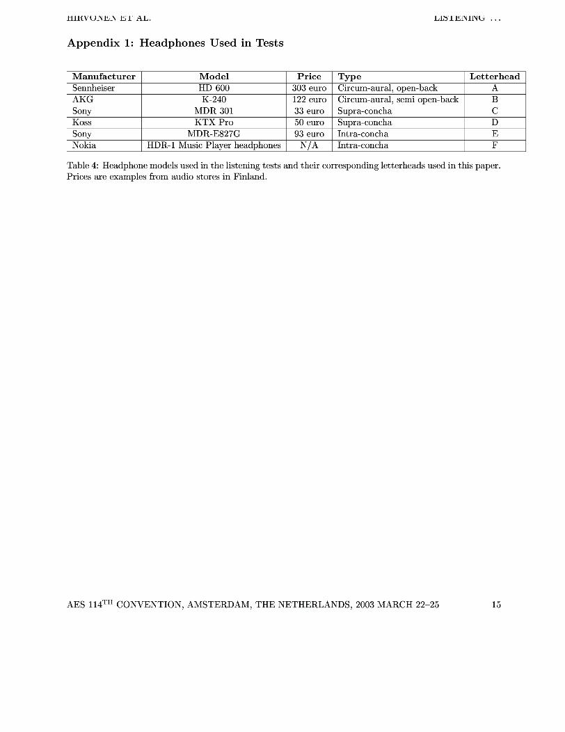
The six headphones used in these tests for both regular listening and recording parts are listed in Table 4 in Appendix 1. Two intra-concha models were included in addition to the four more conventional headphones. The devices were selected so that all had unique but not too recognizable sound coloration properties.

Preliminary pilot tests done prior to this investigation showed that the six headphone models used here were suitable for this purpose. Initially, we examined eight headphone models in listening tests similar to those presented here. From these eight, two models were discarded because the subjects could associate their headphone recordings to the real devices. This was not the purpose of the listening tests because it violates the double-blind conditions of the test done with the recordings. The remaining six headphones had distinct timbres without none of them standing out from the others too strongly.

3.2 Sound Samples Used in the Test

ITU recommends that the programme material used in listening tests should consist of critical material [I]. The material should stress the system under test. Consequently, audio devices such as headphones are usually tested with diverse music material.

For the purposes of this research, however, speech was deemed to be more suitable as the material of choice. The main reason for this was that the initial motivation of our research was to determine the suit- ability of HATS when recording band-limited signals used in telecommunication. Furthermore, the type 3.3 ear simulator we used with the Bryel & Kjaer (B&K) HATS is not specified for frequencies above 8 kHz. This frequency limitation was thought to be unsuitable for music signals. Investigating the recording and simulation method with band-limited speech was thus deemed to be more important than with music.

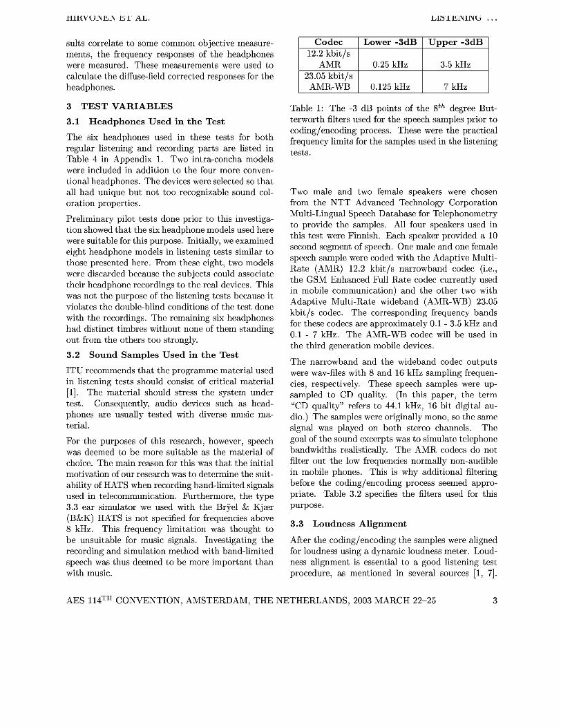
12.2 kbit/s 0.25 kHz 3.5 kHz

23.05 kbit/s 7 kHz

Table 1: The -3 dB points of the 8th degree But- terworth filters used for the speech samples prior to coding/encoding process. These were the practical frequency limits for the samples used in the listening tests.

Two male and two female speakers were chosen from the NTT Advanced Technology Corporation Multi-Lingual Speech Database for Telephonometry to provide the samples. All four speakers used in this test were Finnish. Each speaker provided a 10 second segment of speech. One male and one female speech sample were coded with the Adaptive Multi- Rate (AMR) 12.2 kbit/s narrowband codec (i.e., the GSM Enhanced Full Rate codec currently used in mobile communication) and the other two with Adaptive Multi-Rate wideband (AMR-WB) 23.05 kbit/s codec. The corresponding frequency bands for these codecs are approximately 0.1 - 3.5 kHz and 0.1 - 7 kHz. The AMR-WB codec will be used in the third generation mobile devices.

The narrowband and the wideband codec outputs were wav-files with 8 and 16 kHz sampling frequencies, respectively. These speech samples were up- sampled to CD quality. (In this paper, the term "CD quality" refers to 44.1 kHz, 16 bit digital audio.) The samples were originally mono, so the same signal was played on both stereo channels. The goal of the sound excerpts was to simulate telephone bandwidths realistically. The AMR codecs do not filter out the low frequencies normally non-audible in mobile phones. This is why additional filtering before the coding/encoding process seemed appro- priate. Table 3.2 specifies the filters used for this purpose.

3.3 Loudness Alignment

After the coding/encoding the samples were aligned for loudness using a dynamic loudness meter. Loud- ness alignment is essential to a good listening test procedure, as mentioned in several sources [I, 71.



However, there exists no standardized methods for the loudness alignment of time-varying sounds. We decided to use the dynamic loudness, i.e., the loudness level that is exceeded 10% of the time during the sound event, as a basis for the alignment.

In practice, the loudness calibration was done as follows: The sound excerpts were divided in frames of 1024 samples (approximately 23 ms) and a Matlab loudness tool developed by Tuomi and Zacharov [8] was used to calculate a loudness value for each frame. This tool uses the Moore loudness model [9]. There was also a 50% overlap to the previous frame. The dynamic loudness value for a sound sample could then be calculated using the loudness-per-frame in- formation. The narrowband and wideband excerpts were gained to be equal based on their dynamic loudness values. The whole process was then repeated for a second time for the aligned samples. The final dynamic loudness variations among the samples were below 1 dB. Although not formally validated, the dynamic loudness meter seemed to produce a good alignment for the samples, based on the subjects' feedback.

We had now obtained loudness-aligned, CD quality speech samples both narrow- and wideband coded/encoded. These samples were used for both tests. No further processing was done for the part with real headphones; only the devices themselves were calibrated and adjusted for loudness (see Sec- tion 3.6). To create the simulations for the recording test, some additional steps were required. This process is described in the next two sections.

3.4 Recording Process

The recording environment used in this test was the small anechoic chamber (lower frequency limit 90 Hz) in the HUT Laboratory of Acoustics and Audio Signal Processing. A B&K HATS model 4128C was placed in the anechoic chamber and each headphone was carefully fitted on it one a t a time. Background noise did not cause problems due to a well-insulated recording environment. The HATS recording microphones are located a t the Drum Reference Point (DRP) of the artificial ear i.e. at the end of the ear canal simulator [5]. The four test samples had been converted to an audio CD. A Sony CD player with Symmetrix 304 headphone amplifier was used to play the samples through the headphones. The

recordings were saved with a computer in CD quality wav- format.

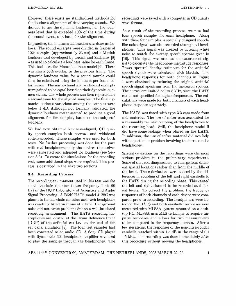
As a result of the recording process, we now had four speech samples for each headphone. Along with these four samples, a specially designed speech- like noise signal was also recorded through all headphones. This signal was created by filtering white noise to match the average speech spectra given in [lo]. This signal was used as a measurement signal to calculate the headphone magnitude responses. Power spectral density estimates for the artificial speech signals were calculated with Matlab. The headphone responses for both channels in Figure 1 were obtained by reducing the original artificial speech signal spectrum from the measured spectra. The curves are limited below 8 kHz, since the HATS ear is not specified for higher frequencies. The calculations were made for both channels of each headphone response separately.

The HATS was fitted with type 3.3 ears made from soft material. The use of softer ears accounted for a reasonably realistic coupling of the headphones to the recording head. Still, the headphone model B did have some leakage when placed on the HATS. In addition, the use of softer material did not help with a particular problem involving the intra-concha headphones.

Spatial deviations on the recordings were the most serious problem in the preliminary experiments. Some of the recordings seemed to emerge from different spatial locations rather than from the middle of the head. These deviations were caused by the differences in coupling of the left and right earshells to the HATS during the recording phase. This caused the left and right channel to be recorded at different levels. To correct the problem, the frequency responses of both channels of each device were compared prior to recording. The headphones were fitted on the HATS and both earshells' responses were measured with MLSSA system mounted on a desk- top PC. MLSSA uses MLS technique to acquire im- pulse responses and allows for two measurements to be compared in the frequency domain. After a few iterations, the responses of the non-intra-concha earshells matched within 1.5 dB in the range of 0.1 - 5 kHz. The recording was done immediately after this procedure without moving the headphones.



Fig. 1: Frequency responses of headphones (from top to down) A, B, C7 D7 E, F measured at the HATS DRP (frequency range of 0.1 - 8 kHz). Measurements for both channels for all headphones are visible .

The intra-concha models were more difficult to fit similarly on the HATS ears; especially the headphone model F suffered from poor coupling. It seemed that the left and right ear of the B&K HATS were slightly different in shape so that the coupling of the intra-concha headphones to the left concha was tighter than to the right one. Intra-concha earshells' responses differed as much as 3.5 dB in the range of 0.1 - 5 kHz, despite of numerous re-fittings. The final channel-comparison measurements can be seen in Figure 1.

Although the background noise was minimized during the recording process, the speech samples were low-pass filtered to remove hiss from the higher frequencies. The passband limits of these filters were 4 and 7 kHz for narrow- and wideband samples, respectively. Although the excerpts had some detectable noise, the overall timbre simulation was deemed to be adequate. At this point, a similar dynamic loudness alignment as before was done for the recorded samples.

3.5 Headphone Compensation

In the recordings test, the subjects listened all the samples through one pair of headphones. The device used for this purpose was the model A in table 4. These headphones were the most expensive and arguably represented the highest quality among the devices used here. Despite of their high quality, the headphones A had an individual spectral coloration effect. This effect needed to be removed by compen- sating the frequency response of headphone model A in the recordings.

A compensation filter was created for this purpose. Since the HATS microphones are located at the DRP of the artificial ears, the measured magnitude response of a headphone represents the combined "headphone-and-ear7' transfer function. We created a filter that inverses the effect of this transfer function for the headphones A. This way the spectral coloration caused by the playback device could be eliminated during the recordings test.



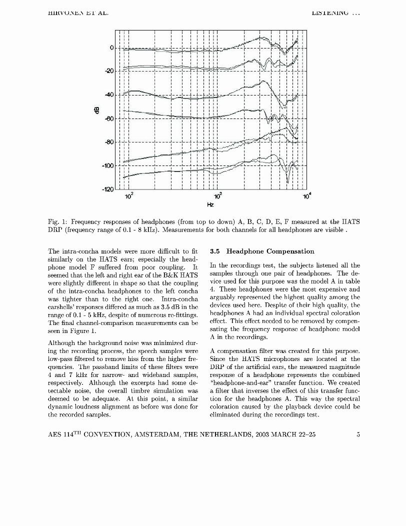
The practical procedure was to measure several headphones of the same type and derive a generic correction for the model A. The results were also used in another project. Three pairs of headphones A were measured with a MLSSA system described in the previous section. Each earshell was measured three times and the headphones were re-fitted between the measurements. The correction was done separately for both channels. The averages of nine responses per channel were used to design a two- channel "inverse headphone model A" IIR filter. All the recorded samples were filtered with the compensation filter after they had been loudness aligned. Theoretically, only the frequency responses of the recorded headphones affected the timbres of the final sounds the subjects listened to. A diagram il- lustrating the test arrangement in both parts can be seen in Figure 2.

3.6 Test Site

The listening tests were done in the listening room of the Laboratory of Acoustics and Audio Signal Pro- cessing at HUT. The room offered ideal conditions for headphone listening and provided a smooth test interface. The GP2 listening test software [ll] was used to implement both tests. The software ran on a Silicon Graphics Octane (SGI) workstation.

All the electrical equipment, such as amplifiers and computers, were located in an isolated control room next to the listening room. The image from the SGI monitor was projected to a video screen in the listening room. Only the headphones, a keyboard, and a mouse were placed inside with the listener. Details about the design and objective measurements of the listening room can be found from [12]. It is safe to say, that there were no problems related to the background noise or other distractions on the listening site.

The test site aimed to be as ergonomic as possible so the subjects would not have to move more than absolutely necessary. The signal from the test computer was routed to two Symmetrix 304 preampli- fiers that were used to drive the headphones. The headphones were laid on a table in the listening room. All brand indicators were covered with tape. Letters A through F were used to identify the devices. The subject controlled the test interface with a mouse and a keyboard.

The loudness of all the samples had been aligned according to their dynamic loudness by the Matlab loudness tool. But this was not yet sufficient because of the impedance differences in the headphones. In consequence, a level alignment was done to the headphones themselves by adjusting the preampli- fier gains. The Matlab loudness tool was used to calibrate the loudness levels when the headphones were driven with the speech-like noise signal introduced earlier. The final listening level was 80 +/- 1.5 phones. The level was constant for all subjects. It must be noted that individual differences in human anatomy make it difficult to align the actual subjective loudness of the headphones, especially the intra- concha models'. There were some remarks consider- ing the alignment but the overall opinion was that the headphones sounded equally loud.

4 EXPERIMENTAL PROCEDURE

4.1 Test Subjects

The 21 subjects who participated in both tests were university students at HUT. All of them had com- pleted at least some of the laboratory's acoustics courses and some had a professional background in audio and acoustics. The gender ratio was rather un- even since only one female subject attended. This was deemed to be an insignificant factor, based on Toole's results [3].

It was decided that a brief training session would be held prior to both parts of the test. Here the concept of timbre was specified and some training samples were presented in order to familiarize the hearing with the tasks ahead. These samples contained seg- ments from all the test samples. No grading was required; rather the idea was to warm up the subjects' hearing, so to speak. It was further emphasized that the grading should be based on timbre alone and not on background noise or other factors. Training was done separately for both sessions. Possible hearing impairments were also inquired and none of the subjects reported one.

Based on commentary after the tests, the majority of the subjects did not recognize any of the headphones by brand. Some subjects, however, reported familiarity to the higher-end models. The presence of visual biasing was of course intentional in the test where the real headphones were listened. But it is



~efldohone compensation

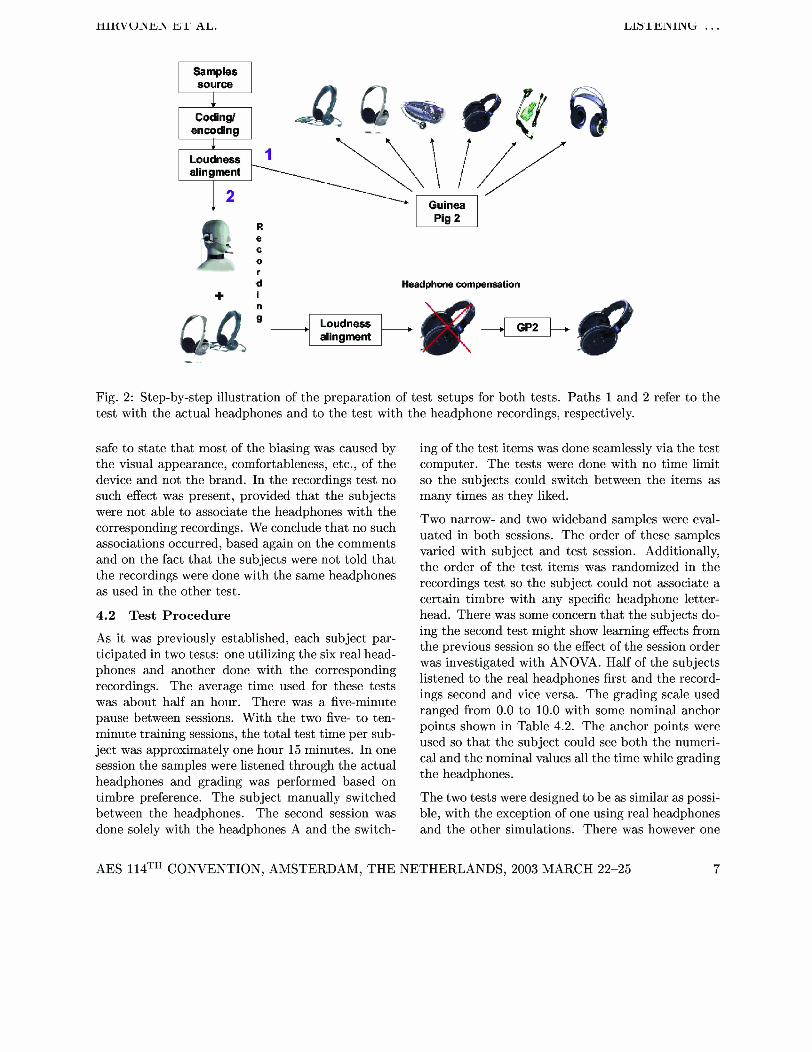
Fig. 2: Step-by-step illustration of the preparation of test setups for both tests. Paths 1 and 2 refer to the test with the actual headphones and to the test with the headphone recordings, respectively.

safe to state that most of the biasing was caused by the visual appearance, comfortableness, etc., of the device and not the brand. In the recordings test no such effect was present, provided that the subjects were not able to associate the headphones with the corresponding recordings. We conclude that no such associations occurred, based again on the comments and on the fact that the subjects were not told that the recordings were done with the same headphones as used in the other test.

4.2 Test Procedure

As it was previously established, each subject participated in two tests: one utilizing the six real headphones and another done with the corresponding recordings. The average time used for these tests was about half an hour. There was a five-minute pause between sessions. With the two five- to ten- minute training sessions, the total test time per subject was approximately one hour 15 minutes. In one session the samples were listened through the actual headphones and grading was performed based on timbre preference. The subject manually switched between the headphones. The second session was done solely with the headphones A and the switch-

ing of the test items was done seamlessly via the test computer. The tests were done with no time limit so the subjects could switch between the items as many times as they liked.

Two narrow- and two wideband samples were evaluated in both sessions. The order of these samples varied with subject and test session. Additionally, the order of the test items was randomized in the recordings test so the subject could not associate a certain timbre with any specific headphone letterhead. There was some concern that the subjects do- ing the second test might show learning effects from the previous session so the effect of the session order was investigated with ANOVA. Half of the subjects listened to the real headphones first and the recordings second and vice versa. The grading scale used ranged from 0.0 to 10.0 with some nominal anchor points shown in Table 4.2. The anchor points were used so that the subject could see both the numeri- cal and the nominal values all the time while grading the headphones.

The two tests were designed to be as similar as possible, with the exception of one using real headphones and the other simulations. There was however one



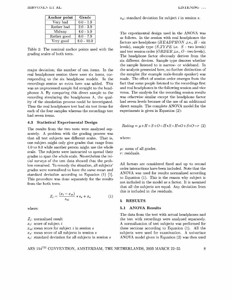
Table 2: The nominal anchor points used with the grading scales of both tests.

Anchor point Very bad

Rather bad Midway

Rather good Very good

major deviation; the number of test items. In the real headphones session there were six items, corresponding to the six headphone models. In the recordings session an extra item was added. This was an unprocessed sample fed straight to the headphones A. By comparing this direct sample to the recording simulating the headphones A, the quality of the simulation process could be investigated. Thus the real headphones test had six test items for each of the four samples whereas the recordings test had seven items.

Grade 0.0 - 1.9 2.0 - 3.9 4.0 - 5.9 6.0 - 7.9 8.0 - 10.0

4.3 Statistical Experimental Design

The results from the two tests were analyzed separately. A problem with the grading process was that all test subjects use different scales. That is, one subject might only give grades that range from 4.0 to 8.0 while another person might use the whole scale. The subjects were instructed to spread their grades to span the whole scale. Nevertheless the initial surveys of the test data showed that the problem remained. To remedy the situation, all subjects' grades were normalized to have the same mean and standard deviation according to Equation (1) [I]. This procedure was done separately for the results from the both tests.

where:

hlS'l'HilWl\ ti . .

ssi: standard deviation for subject i in session s.

The experimental design used in the ANOVA was as follows. In the session with real headphones the factors are headphone (HEADPHON ,i.e., H - six levels), sample type ( S m E i.e. S - two levels) and test session order (ORDER ,i.e., 0 - two levels). The headphone factor obviously derives from the six different devices. Sample type denotes whether the sample listened to is narrow- or wideband. In the analysis presented here, no further distinction of the samples (for example male-female speaker) was made. The effect of session order emerges from the fact that some people listened to the recordings first and real headphones in the following session and vice versa. The analysis for the recording session results was otherwise similar except the headphone factor had seven levels because of the use of an additional direct sample. The complete ANOVA model for the experiments is given in Equation (2):

Rating = p+H+S+O+H*S+H*O+S*O+r (2)

where:

p: mean of all grades. r: residuals.

All factors are considered fixed and up to second order interactions have been included. Note that the ANOVA was used for results normalized according to Equation (1). This is the reason why subject is not included in the model as a factor. It is assumed that all the subjects are equal. Any deviation from this is included in the residuals.

5 RESULTS

5.1 ANOVA Results

2,: normalized result xi: score of subject i x.i: mean score for subject i in session s x.: mean score of all subjects in session s s.: standard deviation for all subjects in session s

The data from the test with actual headphones and the test with recordings were analyzed separately. A normalization of test subjects was performed for these sections according to Equation (1). All the subjects were used for examination. A univariate ANOVA model given in Equation (2) was then used



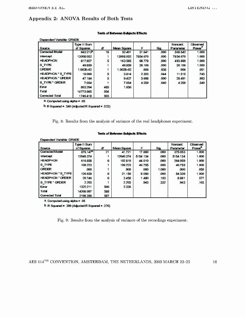
for analysis. The ANOVA tables are presented in Appendix 2.

The significant (p<0.05) factors were:

Real headphones-test: HEADPHON, S-TYPE, H E A D P H O N * SrYPE, H E A D P H O N * ORDER, S-TYPE * ORDER.

HEADPHON, S-TYPE, H E A D P H O N * S-TYPE.

5.2 Comparison of Grades Given to Real Headphones and Recordings

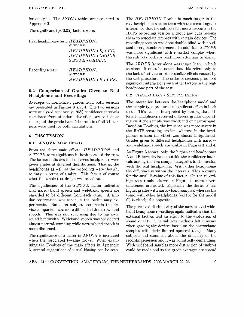
Averages of normalized grades from both sessions are presented in Figures 3 and 4. The two sessions were analyzed separately. 95% confidence intervals calculated from standard deviations are visible a t the top of the grade bars. The results of all 21 subjects were used for both calculations.

6 DISCUSSION

6.1 ANOVA Main Effects

From the three main effects, H E A D P H O N and S-TYPE were significant in both parts of the test. The former indicates that different headphones were given grades a t different distributions. That is, the headphones as well as the recordings were thought to vary in terms of timbre. This fact is of course what the whole test design was based on.

The H E A D P H O N F-value is much larger in the real headphones session than with the recordings. It is assumed that the subjects felt more insecure in the HATS recordings session without any cues helping them to associate timbres with certain devices. The recordings session was done double-blind with no visual or ergonomic references. In addition, S-TYPE was more significant with recorded samples where the subjects perhaps paid more attention to sound.

The ORDER factor alone was insignificant in both sessions. It must be noted that this refers only to the lack of fatigue or other similar effects caused by the test procedure. The order of sessions produced significant interactions with other factors in the real- headphone part of the test.

6.2 H E A D P H O N * S^TYPE Factor

The interaction between the headphone model and the sample type produced a significant effect in both tests. This can be interpreted by stating that different headphones received different grades depending on if the sample was wideband or narrowband. Based on F-values, the influence was more severe in the HATS-recording session, whereas in the headphones session the effect was almost insignificant. Grades given to different headphones with narrow- and wideband speech are visible in Figures 3 and 4.

As Figure 3 shows, only the higher-end headphones A and B have deviation outside the confidence intervals among the two sample categories in the session with the real headphones. With other headphones the difference is within the intervals. This accounts for the small F-value of this factor. On the recordings test results shown in Figure 4, more severe

The significance of the S-TYPE factor indicates differences are noted. Especially the device F has that narrowband speech and wideband speech are higher grades with narrowband samples, whereas the regarded to be different from each other. A sim- trend with other headphones (except for the model ilar observation was made in the preliminary ex- C) is clearly the opposite. periments. Based on subjects comments the device comparison was more difficult with narrowband speech. This was not surprising due to narrower sound bandwidth. Wideband speech was considered almost natural-sounding while narrowband speech is more discerned.

The significance of a factor in ANOVA is increased when the associated F-value grows. When examining the F-values of the main effects in Appendix 3, several suggestions of visual biasing can be seen.

The perceived dissimilarity of the narrow- and wideband headphone recordings again indicates that the external factors had an effect to the evaluation of sound quality. The subjects perhaps felt insecure when grading the devices based on the narrowband samples with their limited spectral range. Many subjects did comment about the difficulty of the recordings-session and it was admittedly demanding. With wideband samples more distinction of timbres could be made and so the grade averages are spread



8~ E all samples

C D E headphone

Fig. 3: Normalized grades of all subjects with different headphones. The 95% confidence intervals are visi at the top of the grade bars.

mall samples Â wideband

Direct A B C D E F

headphone

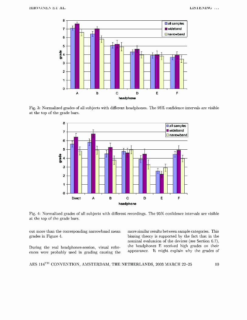
Fig. 4: Normalized grades of all subjects with different recordings. The 95% confidence intervals are visible at the top of the grade bars.

out more than the corresponding narrowband mean more similar results between sample categories. This grades in Figure 4. biasing theory is supported by the fact that in the

nominal evaluation of the devices (see Section 6.7),

During the real headphones-session, visual refer- the headphones E received high grades on their

ences were probably used in grading causing the appearance. It might explain why the grades of



this model have decreased relatively in the HATS recordings-session. I done first

I done second Based on the subjects' comments, wideband speech was generally thought to be almost natural-sounding I

whereas narrowband speech was considered to be 8 5 -

' h I T

clearly unnatural. Grade deviations between sam- o> 4 pie categories in Figures 3 and 4, especially with the 3 . J higher-end headphones, support this viewpoint. We 2. conclude that wideband coded speech differs from 1 . the old telephone-band (i.e. narrowband coded) speech perceptually. Thus the assessment of sound C D quality done with narrowband speech should not be headphone

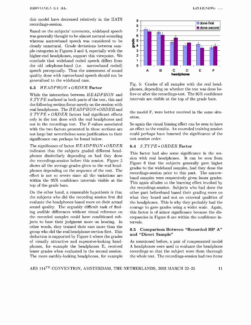
generalized to the wideband case. Fig. 5: Grades of all samples with the real head-

6.3 HEADPHON * ORDER Factor phones, depending on whether the test was done be- While the interaction between HEADpHON and fore or after the recordings-test. The 95% confidence S-TYpE surfaced in both parts of the test, this and intervals are visible at the top of the grade bars. the following section focus merely on the session with real The HEADpHoN*oRDERand

the model F, were better received in the same situ- S-TYPE * ORDER factors had significant effects only in the test done with the real headphones and ation.

not in the recordings test. The F-values associated So again the visual biasing effect can be seen to have with the two factors presented in these sections are an effect to the results. An extended training session not large but nevertheless some justification to their could perhaps have lessened the significance of the significance can perhaps be found below. test session order.

The significance of factor HEADPHON *ORDER 6.4 S-TYPE * ORDER Factor indicates that the subjects graded different headphones dissimilarly depending on had they done the recordings-session before this session. Figure 5 shows all the average grades given to the real headphones depending on the sequence of the test. The effect is not so severe since all the variations are within the 95% confidence intervals visible at the top of the grade bars.

On the other hand, a reasonable hypothesis is that the subjects who did the recording session first did evaluate the headphones based more on their actual sound quality. The arguably difficult task of finding audible differences without visual reference on the recorded samples could have conditioned subjects to base their judgment more on hearing. In other words, they trained their ears more than the group who did the real headphone-section first. This deduction is supported by Figure 5 where the grades of visually attractive and expensive-looking headphones, for example the headphones E, received lesser grades when evaluated in the second session. The more earthly-looking headphones, for example

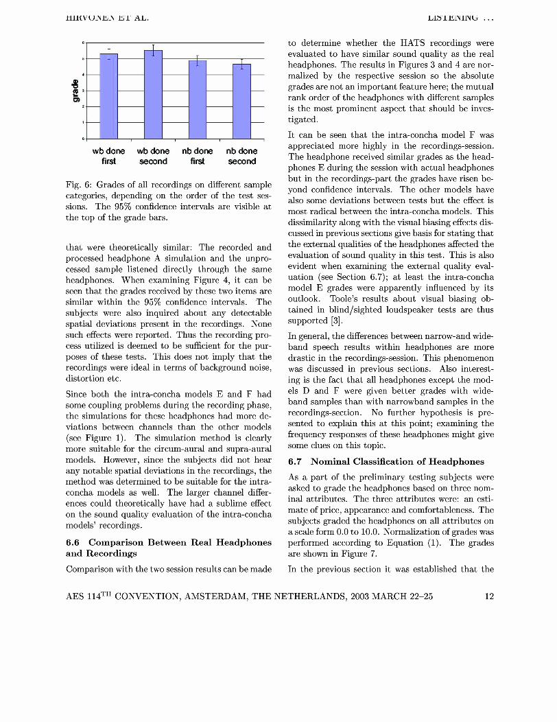
This factor had also some significance in the session with real headphones. It can be seen from Figure 6 that the subjects generally gave higher grades to the wideband samples, had they done the recordings-session prior to this part. The narrowband samples were respectively given lesser grades. This again alludes to the learning effect invoked by the recordings-session. Subjects who had done the other part beforehand based their grading more on what they heard and not on external qualities of the headphones. This is why they probably had the courage to gave grades using a wider scale. Again, this factor is of minor significance because the dis- crepancies in Figure 6 are within the confidence intervals.

6.5 Comparison Between "Recorded HP A" and "Direct Sample"

As mentioned before, a pair of compensated model A headphones were used to evaluate the headphone recordings so that the subject wore them thorough the whole test. The recordings-session had two items



wbdone wb done nbdone nb done first second first second

Fig. 6: Grades of all recordings on different sample categories, depending on the order of the test sessions. The 95% confidence intervals are visible a t the top of the grade bars.

that were theoretically similar: The recorded and processed headphone A simulation and the unprocessed sample listened directly through the same headphones. When examining Figure 4, it can be seen that the grades received by these two items are similar within the 95% confidence intervals. The subjects were also inquired about any detectable spatial deviations present in the recordings. None such effects were reported. Thus the recording process utilized is deemed to be sufficient for the purposes of these tests. This does not imply that the recordings were ideal in terms of background noise, distortion etc.

Since both the intra-concha models E and F had some coupling problems during the recording phase, the simulations for these headphones had more deviations between channels than the other models (see Figure 1). The simulation method is clearly more suitable for the circum-aural and supra-aural models. However, since the subjects did not hear any notable spatial deviations in the recordings, the method was determined to be suitable for the intra- concha models as well. The larger channel differences could theoretically have had a sublime effect on the sound quality evaluation of the intra-concha models' recordings.

to determine whether the HATS recordings were evaluated to have similar sound quality as the real headphones. The results in Figures 3 and 4 are normalized by the respective session so the absolute grades are not an important feature here; the mutual rank order of the headphones with different samples is the most prominent aspect that should be investigated.

It can be seen that the intra-concha model F was appreciated more highly in the recordings-session. The headphone received similar grades as the headphones E during the session with actual headphones but in the recordings-part the grades have risen beyond confidence intervals. The other models have also some deviations between tests but the effect is most radical between the intra-concha models. This dissimilarity along with the visual biasing effects discussed in previous sections give basis for stating that the external qualities of the headphones affected the evaluation of sound quality in this test. This is also evident when examining the external quality evaluation (see Section 6.7); at least the intra-concha model E grades were apparently influenced by its outlook. Toole's results about visual biasing obtained in blindlsighted loudspeaker tests are thus supported [3].

In general, the differences between narrow-and wideband speech results within headphones are more drastic in the recordings-session. This phenomenon was discussed in previous sections. Also interesting is the fact that all headphones except the models D and F were given better grades with wideband samples than with narrowband samples in the recordings-section. No further hypothesis is presented to explain this at this point; examining the frequency responses of these headphones might give some clues on this topic.

6.7 Nominal Classification of Headphones

As a part of the preliminary testing subjects were asked to grade the headphones based on three nominal attributes. The three attributes were: an esti- mate of price, appearance and comfortableness. The subjects graded the headphones on all attributes on a scale form 0.0 to 10.0. Normalization of grades was

6.6 Comparison Between Real Headphones performed according to Equation (1). The grades and Recordings are shown in Figure 7.

Comparison with the two session results can be made In the previous section it was established that the



1 price appearance confortableness

A B c D E headphone

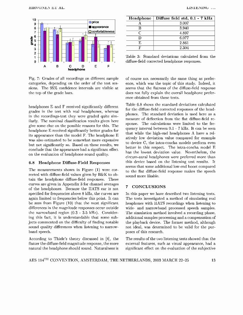
Fig. 7: Grades of all recordings on different sample categories, depending on the order of the test sessions. The 95% confidence intervals are visible a t the top of the grade bars.

headphones E and F received significantly different grades in the test with real headphones, whereas in the recordings-test they were graded quite similarly. The nominal classification results given here give some clue on the possible reasons for this. The headphone E received significantly better grades for its appearance than the model F. The headphone E was also estimated to be somewhat more expensive but not significantly so. Based on these results, we conclude that the appearance had a significant effect on the evaluation of headphone sound quality.

6.8 Headphone Diffuse-Field Responses

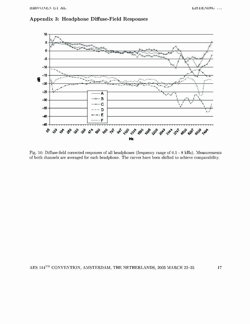
The measurements shown in Figure (1) were corrected with diffuse-field values given by B&K to ob- tain the headphone diffuse-field responses. These curves are given in Appendix 3 for channel averages of the headphones. Because the HATS ear is not specified for frequencies above 8 kHz, the curves are again limited to frequencies below this point. It can be seen from Figure (10) that the most significant differences in the magnitude responses occur outside the narrowband region (0.3 - 3.5 kHz). Consider- ing this fact, it is understandable that some subjects commented on the difficulty of finding notable sound quality differences when listening to narrowband speech.

According to Thiele's theory discussed in [4], the flatter the diffuse-field magnitude response, the more natural the headphone should sound. Naturalness is

Table 3: Standard deviations calculated from the diffuse-field corrected headphone responses.

Headphone A B C D E F

of course not necessarily the same thing as preference, which was the topic of this study. Indeed, it seems that the flatness of the diffuse-field response does not fully explain the overall headphone preference obtained from these tests.

Diffuse field std, 0.1 - 7 kHz 3.007 3.940 4.897 6.077 2.861 2.304

Table 6.8 shows the standard deviations calculated for the diffuse-field corrected responses of the headphones. The standard deviation is used here as a measure of deflection from the flat diffuse-field response. The calculations were limited to the frequency interval between 0.1 - 7 kHz. It can be seen that while the high-end headphones A have a relatively low deviation value compared for example to device C, the intra-concha models perform even better in this respect. The intra-concha model E has the lowest deviation value. Nevertheless, the circum-aural headphones were preferred more than this device based on the listening test results. It seems that some additional low-end boost compared to the flat diffuse-field response makes the speech sound more likable.

7 CONCLUSIONS

In this paper we have described two listening tests. The tests investigated a method of simulating real heaphones with HATS recordings when listening to wide- and narrowband processed speech samples. The simulation method involved a recording phase, additional samples processing and a compensation of the playback device. The former method, although not ideal, was determined to be valid for the purposes of this research.

The results of the two listening tests showed that the external features, such as visual appearance, had a significant effect on the evaluation of the subjective



sound quality of the headphones. There were many 9 REFERENCES similarities among the preference orders obtained from the two tests. In spite of that, statistical analysis showed significant differences beyond the confidence intervals in case of one intra-concha model (the headphones E). Thus the simulation method, although promising, cannot be validated based on the results presented here.

The overall preference order of the headphones was as expected prior to the test. The more expensive circum-aural models prevailed over the supra-aural and the intra-concha models. However, the listening tests presented in this paper were done in a noise- less environment. Also, the subjects were asked to base their grading only on sound color. It is possible that the headphone preferences would change in the presence of background noise or in other conditions where the intelligibility of speech is a key factor.

The flatness of the headphone diffuse-field responses does not fully correlate with the obtained subjective preference results. In the light of the results, an additional lower frequency enhancement compared to the flat diffuse-field response seems to make speech sound more pleasant. The main differences in the headphone magnitude responses occur in the frequency range above 3.5 kHz i.e. outside the narrowband area.

Narrowband coded speech was concluded to differ perceptually from wideband coded speech. Based on the subjects7 comments wideband speech is considered almost natural-sounding, whereas narrowband speech is clearly unnatural.

8 ACKNOWLEDGMENTS

This research was funded by the Nokia Foundation. Many persons from Nokia Mobile Phones and from Nokia Research Center supplied vast amounts of both equipment and expertise during the course of this research. The authors especially wish to thank Mr. Gaetan Lorho, Mr. Ossi Miknpaa, Dr. Nick Zacharov and Dr. Ville-Veikko Mattila for their help. Also, Dr. Ville Pulkki from HUT Laboratory of Acoustics and Audio Signal Processing assisted with the practical listening room arrangements. Fi- nally, the test subjects deserve commendation for their efforts.

International Telecommunications Union, ITU- R Recommendation BS.1116, 1994 - 1997. S. Bech, "Quantification of Subwoofer Require- ments, Part 11: The Influence of Lower System Cut-Off Frequency and Slope and Pass-Band Amplitude and Group Delay Ripple", AES 10gh Convention, Preprint No. 5199, 2000.

[3] F. Toole and S. E. Olive, "Hearing is Believ- ing vs. Believing is Hearing: Blind vs. Sighted Listening Tests, and Other Interesting Things", AES 97th Convention, Preprint No. 3894, 1994.

[4] G. Thiele, "On the Standardization of the Fre- quency Response of the High-Quality Studio headphones", J. Audio Eng. Soc. vol. 34, No. 12, 1986.

[5] International Telecommunications Union, ITU- R Recommendation BS. 708, 1990.

[6] T. Hirvonen, Headphone Listening Test Meth- ods, M.Sc. Thesis, Helsinki University of Tech- nology, 2002.

[7] A. Gabrielson and B. Lindstrom, "Perceived Sound Quality of High-Fidelity Loudspeakers", J. Audio Eng. Soc. vol. 33, No. 112, 1985.

[8] 0. Tuomi and N. Zacharov "A Real-Time Bin- aural Loudness Meter" Presented at the 13gh meeting of the Acoust. Soc. Am. Atlanta, USA, June, 2000.

[9] B. Moore et al., "A Model for the Prediction of Thresholds, Loudness and Partial Loudness", J. Audio Eng. Soc. vol. 45, No. 4, 1997.

[lo] K. Pearsons et al. "Speech Levels in Vari- ous Noise Environments" U.S. Environmental Protection Agency Report EPA-60011-77-025, 1977.

[ll] J . Hynninen and N. Zacharov, "GP 2: A Generic Subjective Test System for Multichan- nel Audio" AES 106th Convention, Preprint No. 4563, 1999.

[12] A. Jiirvinen, Kuunteluhuoneen Suunnittelu ja Mallinnus, M.Sc. Thesis, Helsinki University of Technology, 1999.



Appendix 1: Headphones Used in Tests

Manufacturer 1 Model 1 Price 1 Type 1 Letterhead

Table 4: Headphone models used in the listening tests and their corresponding letterheads used in this paper. Prices are examples from audio stores in Finland.

Sennheiser AKG Sony Koss Sony Nokia


HD 600 1 303 euro 1 Circum-aural, open-back K-240

MDR 301 KTX Pro

MDR-E827G HDR-1 Music Player headphones

A 122 euro 33 euro 50 euro 93 euro

NIA

. - Circum-aural, semi open-back Supra-concha Supra-concha Intra-concha Intra-concha

B C D E F

HlKVUl\El\ El' Ah.

Appendix 2: ANOVA Results of Both Tests

3 m c.me&dM& I h r n HE W H O N 3-WW o m HEWHON * S-WE HEWHON * CRIER 3 - W E * CRIER Emm T0.M cure&d T0.M

Fig. 8: Results from the analysis of variance of the real headphones experiment.

l W . 3 7 4 1 HENFHON 616.- 6 3 - W E 1 m . m 1 O m .m 1 HENFHON - 3 - W E I%.= 6

HENFHON *-R 20.7d6 6

3-WE * -R 2 . m 1 Emm I =.?I I 333 T0.M 14266.W7 s&l w&d T0.M 2 1 w . w 5B7

a. mi-^ dm = .w b. R Fqmd = .m ~~~ R 3-d = .3?6,l

Fig. 9: Results from the analysis of variance of the recordings experiment.

AES l1dTH CONVENTION, AMSTERDAM, THE NETHERLANDS, 2003 MARCH 22-25

HlKVUl\El\ El' Ah.

Appendix 3: Headphone Diffuse-Field Responses

Fig. 10: Diffuse-field corrected responses of all headphones (frequency range of 0.1 - 8 kHz). Measurements of both channels are averaged for each headphone. The curves have been shifted to achieve comparability.

AES l1dTH CONVENTION, AMSTERDAM, THE NETHERLANDS, 2003 MARCH 22-25

Documents

Audio Engineering Society convention Pa per 5736users.spa.aalto.fi/mak/PUB/AES114_Hirvonen.pdf · Audio Engineering Society convention Pa per 5736 I ... (AMR) 12.2 kbit/s ... ity