ATMOSPHERIC CONVECTION WITH CONDENSATION OF THE MAJORCOMPONENT.

T. Yamashita, Department of Cosmosciences, Hokkaido University, Japan (yamasita@ep.sci.hokudai.ac.jp), M.Odaka, Department of Cosmosciences, Hokkaido University, Japan, K. Sugiyama, Center for Planetary Science(CPS)/ Institute of Low Temperature Science, Hokkaido University, Japan, K. Nakajima, Department of Earth and PlanetarySciences, Faculty of Sciences, Kyushu University, Japan, M. Ishiwatari, CPS / Department of Cosmosciences,Graduate School of Science, Hokkaido University, Japan, Y.O. Takahashi, CPS / Department of Earth and PlanetarySciences, Kobe University, Japan, Y.­Y. Hayashi, CPS / Department of Earth and Planetary Sciences, Kobe University,Japan.

Introduction

In Martian atmosphere, atmospheric major component,CO2, condenses. In current Martian polar regions, CO2

ice clouds are known to exist, and there is a possibil­ity that these clouds are formed by convective motion(Colaprete et al., 2003). Pollack et al.(1987) and Kast­ing(1991) proposed that the early Martian atmospherewas thicker than present one, and that large amounts ofCO2 ice cloud existed. Studies on the early Martianclimate suggested that the scattering greenhouse effectof CO2 ice clouds had a significant effect on the climate(Forget and Pierrehumbert, 1997: Mitsuda, 2007).

In a system whose major component condenses, thedegrees of freedom for thermodynamic variables de­generate when supersaturation does not occur. Due todegeneracy of degree of freedom, temperature profile ofascent region must be equal to that of descent region,and air parcel can not obtain buoyancy. Colaprete et al.(2003) performed calculations and showed that moistconvection develops when supersaturation occurs, be­cause the supersaturation will permit the temperatureprofile to deviate from the thermodynamical equilib­rium. Laboratory experiments and observations fromorbiters suggested existence of highly supersaturatedregions in Martian atmosphere (Glandorf et al., 2002:Colaprete et al., 2003).

However, the model used by Colaprete et al. (2003)was vertical one dimensional, and there was an uncer­tainty in the parameterizations related to the effects ofentrainment and pressure gradient. In order to investi­gate atmospheric convective structure in various planets,we have been developing a two­dimensional cloud con­vection model (e.g., Nakajima et al, 2000: Odaka etal., 2006: Sugiyama et al., 2009). Odaka et al. (2006)incorporated the effects of condensation of major com­ponent into the cloud convection model, and performednumerical experiments of ascending hot plume as a testcalculation under Martian atmospheric condition. Weincorporated a simple radiation scheme in which heatingand cooling is balanced, and improve the condensationscheme in order to allows for supersaturation to occur.In this study, we perform a long­time numerical sim­ulation of convection with condensation of the majorcomponent using the cloud convection model. In our

calculation, the critical saturation ratio Scr is set to be1.0. The purpose of this study is to investigate cloudstructure in statistical equilibrium states and whethermoist convection can develop in the case of Scr = 1.0.

Model description

We assume that atmosphere consists entirely of CO2.The governing equations are the quasi­compressible equa­tions by Klemp and Wilhelmson(1978) with additionalterms representing major component condensation (Odakaet al., 2005). The model is two­dimensional in the hori­zontal and vertical directions. The equations of motion,the pressure equation, the thermodynamic equation, andthe conservation law for cloud are written as

du′

dt= −cpθ

∂π′

∂x+ Dm(u′), (1)

dw′

dt= −cpθ

∂π′

∂z+ g

θ′

θ+ Dm(w′), (2)

∂π′

∂t+

Rπ

cvρθ

[∂(ρθu′)

∂x+

∂(ρθw′)

∂z

]=

Rπ

cvρ

(L

cpθπ− 1

)Mc +

R

cvθ(Qdis + Qrad) ,(3)

dθ′

dt+ w′ ∂θ

∂z=

1

π

(LMc

ρcp+ Qdis + Qrad

)+Dh(θ′), (4)

∂ρ′s

∂t+

∂(ρ′su

′)

∂x+

∂(ρ′sw

′)

∂z= Mc + Dh(ρs), (5)

where

d

dt=

∂

∂t+ u′ ∂

∂x+ w′ ∂

∂z, (6)

D∗(·) =∂

∂x

[K∗

∂(·)∂x

]+

1

ρ

∂

∂z

[ρK∗

∂(·)∂z

]. (7)

u and w are horizontal and vertical component of ve­locity, respectively. ρ is gas density, ρs is cloud den­sity, and T is temperature. π is the Exner function:π = (p/p0)

R/cp , where p is pressure, and p0 is surfacepressure. θ is potential temperature: θ = T/π. Over­bar denotes the basic state which depends only on height,and prime denotes the perturbation component. Km and

Kh are eddy coefficients for momentum and scalar vari­ables, respectively. Qdis is heating rate of dissipation.Km, Kh and Qdis are calculated by using 1.5 order clo­sure (Klemp and Wilhelmson, 1978). Qrad is radiativeheating rate, Mc is condensation rate, and L is latentheat of fusion. cp and cv are the specific heat at constantpressure and volume, respectively. R is the gas constantfor unit mass, g is gravitational acceleration.

We do not calculate radiation transfer explicitly, butwe give horizontally uniform heating and cooling. Cool­ing rate is fixed at constant value qcool, and heating rateqheat(t) is adjusted to retain

∫ zt

zbρQraddz = 0, where zb,

zt are lower and upper levels of computational domain.Then Qrad is given by

Qrad(z, t) =

{qheat(t), (z1 ≤ z ≤ z2)qcool, (z3 ≤ z ≤ z4)0, (otherwise)

(8)

where z1, z2 are lower and upper levels of cooling layer,and z3, z4 are lower and upper levels of heating layer.qheat(t) is given by

qheat(t) = −qcool ×

∫ z4

z3ρdz∫ z2

z1ρdz

. (9)

Neither surface fluxes of momentum nor heat are con­sidered in our model.

Condensation of CO2 occurs when saturation ratioS = p/p∗ exceeds critical saturation ratio Scr, where p∗is saturated vapor pressure. p∗ is given by

p∗ = exp(Aant −

Bant

T

), (10)

where Aant = 27.4, Bant = 3103 K (The society ofchemical engineers of Japan, 1999). We assume thatcloud particles grow by diffusion process, and the growthby coalescence process is not considered. Mc is ex­pressed by Tobie et al. (2003)’s formulation with athreshold for inhibiting unphysical condensation;

Mc =4πrNkdRT 2

L2(S − 1)

if

{S > Scr

or S ≤ 1, ρs 6= 0or 1 < S ≤ Scr, ρs > ε,

(11)

where r is cloud particle radius(determined by (12)), Nis number density of condensation nuclei, and kd is heatconduction coefficient. We use the value of kd = 4.8 ×10−3 W K−1 m−1 (Tobie et al., 2003). ε is a thresholdconstant for inhibiting unphysical condensation whichcan occur when S is large. From (10) and the Clausius­Clapeyron equation, L is constant value: L = BantR.

We assume that r in one grid domain are constant,and r is expressed by ρ′

s and rd :

r =

(r3

d +3ρ′

s

4πNρI

)1/3

, (12)

where ρI is the density of CO2 ice. ρI is 1.565 × 103

kg/m3 (NAOJ, 2004), rd is 0.1 µm, and number of con­densation nucleus per unit mass of air N/ρ is 5.0×108

kg−1 (Tobie et al., 2003).In this simulation, we do not consider falling of cloud

particle and drag force due to cloud particles.For space discretization, we use fourth order cen­

tered difference for advection terms, and second ordercentered difference for the other terms. Solving theadvection term of cloud density by using centered dif­ference causes negative cloud density. When negativecloud density occurs in a grid point, positive cloud den­sity is transferred from surrounding points to the pointso that the cloud density at the point is zero.

For saving computational resources, time­splittingmethod is used. The terms associated with sound waveand condensation are treated by the HE­VI scheme usinga short time step. In the horizontal and vertical direction,Euler and Crank­Nicolson scheme are used, respectively.The other terms are treated by the leap­frog scheme withAsselin time filter(Asselin, 1972) using a long time step.The filter coefficient is 0.1. Artificial viscosity terms areintroduced for the sake of calculation stability.

Developed numerical models and documents are avail­able in http://www.gfd­dennou.org/library/deepconv/.

Numerical configuration

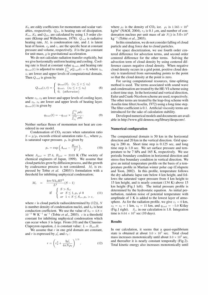
The computational domain is 50 km in the horizontaldirection and 20 km in the vertical direction. Grid spac­ing is 200 m. Short time step is 0.125 sec, and longtime step is 1.0 sec. We set surface pressure and tem­perature to be 7 hPa and 165 K, respectively. We useperiodic boundary condition in horizontal direction andstress­free boundary condition in vertical direction. Wegive an initial temperature profile on the basis of a tem­perature profile in Martian winter polar cap (Colapreteand Toon, 2002). In this profile, temperature followsthe dry adiabatic lapse rate below 4 km height, and fol­lows the saturated vapor pressure from 4 km height to15 km height, and is nearly constant (134 K) above 15km height (Fig.1 left). The initial pressure profile isdetermined by the hydrostatic equation. As initial per­turbation, random noise of potential temperature withamplitude of 1 K is added to the lowest layer of atmo­sphere. As for the radiation profile, we give z1 = 0 km,z2 = z3 = 1 km, z4 = 15 km, and qcool = −5.0 K/day(Fig.1 right). Scr in our calculation is 1.0. Integrationtime is 8.64 × 105 sec (10 days).

Results

In our calculation, it seems that a quasi­equilibriumstate is obtained at about 3.0 × 105 sec. Total cloudmass increases monotonically until about 3.0 × 105 sec,and thereafter it is nearly constant temporally (Fig.2).Total kinetic energy also increases monotonically until

about 3.0 × 105 sec, and it is nearly constant after thetime(Figure not shown).

We describe here time evolution of cloud density andvertical velocity. Fig.3a, 3b and 3c show distributionsof cloud density at 2.16× 104, 8.64× 104 and 3.03× 105

sec, respectively. Fig.4a, 4b and 4c show distributions ofvertical velocity at 2.16× 104, 8.64× 104 and 3.03× 105

sec, respectively. In the early stage, isolated clouds areformed in ascent regions near 6 km height(Fig.3a, 4a).Thereafter, vertical velocity and cloud density increase,and the clouds grow up vertically(Fig.3b, 4b). Verticalvelocity continues to increase until cloud distributionbecomes horizontally uniform(Fig.3c, 4c), and there­after becomes nearly constant temporally. After about3.03 × 105 sec, the region above 7 km level is coveredwith clouds. One­cell circulation in which maximumvertical velocity is about 15 m/sec develops in the cloudlayer. In the quasi­equilibrium state, around 7 kmheight, the cloud layer is sustained by the balance ofnegative contribution of evaporation and positive contri­bution of advection. At altitudes above 7 km, the cloudlayer is sustained by the balance of negative contributionof advection and positive contribution of condensation.

Concluding Remarks

Our calculation shows that moist convection does de­velop in the case of Scr = 1.0 (Fig.3b). This result isdifferent from the discussion by Colaprete et al. (2003)that moist convection does not develop for Scr = 1.0. Inorder to investigate the mechanism for development ofthe moist convection, detailed analysis will be required.

For further works, we are going to perform param­eter sweep experiments for Scr, and calculations withconsidering the falling of cloud particles. Since nu­merical experiments of cloud convection such as Naka­jima et al.(1998) showed that the falling of cloud par­ticles affects the convective structure, calculations withconsidering these effects are essential to investigate thestructure of the convection which is established througha large number of life cycles of convective cloud ele­ments.

Acknowledgement

Figures are plotted by using the softwares developedby Dennou Ruby Project (http://ruby.gfd­dennou.org/).Numerical calculations are performed by the SX8­R ofthe NIES supercomputer system.

References

Asselin, R., 1972: Frequency filter for time integrations,Mon. Wea. Rev., 100, 487–490.

Colaprete, A., Toon, O. B., 2002: Carbon dioxide snowstorms during the polar night on Mars, J. Geophys.Res., 107, 5051, doi:10.1029/2001JE001758.

Colaprete, A., Haberle, R. M., Toon, O. B., 2003: For­mation of convective carbon dioxide clouds near thesouth pole of Mars, J. Geophys. Res., 108(E7), 5081,doi:10.1029/2003JE002053

Forget, F., Pierrehumbert, R. T., 1997: Warming earlyMars with carbon dioxide clouds that scatter infraredradiation, Science, 278, 1273–1276.

Glandorf, D. L., Colaprete, A., Tolbert, M. A., Toon,O. B., 2002: CO2 snow on Mars and early Earth:experimental constraints, Icarus, 160, 66–72.

Kasting, J. F., 1991: CO2 condensation and the climateof early Mars, Icarus, 94, 1–13.

Klemp, J. B., Wilhelmson, R. B., 1978: The simulationof three­dimensional convective storm dynamics, J.Atmos. Sci., 35, 1070–1096.

Mitsuda, C., 2007: The greenhouse effect of radiativelyadjusted CO2 ice cloud in a Martian paleoatmosphere(in Japanese), Doctoral thesis, Hokkaido Univ.,115pp.

Nakajima, K., Takehiro, S., Ishiwatari, M., Hayashi,Y.­Y., 1998: Cloud convections in geophysical and plan­etary fluids(in Japanese), Nagare Multi.,http://www2.nagare.or.jp/mm/98/nakajima/index.htm

Nakajima, K., Takehiro, S., Ishiwatari, M., Hayashi,Y.­Y., 2000: Numerical modeling of Jupiter’s moist con­vection layer, Geophys. Res. Lett., 27, 3129–3132.

National Astronomical Observatory of Japan, 2004: Chrono­logical scientific tables (in Japanese), Maruzen, 1015pp.

Odaka, M., Kitamori, T., Sugiyama, K., Nakajima, K.,Takahashi, Y. O., Ishiwatari, M., Hayashi, Y.­Y., 2005:A formulation of non­hydrostatic model for moist con­vection in the Martian atmosphere, Proc. of the 38 thISAS Lunar and Planetary Symposium, 173–175.

Odaka, M., Kitamori, T., Sugiyama, K., Nakajima, K.,Hayashi, Y.­Y., 2006: A numerical simulation of Mar­tian atmospheric moist convection (in Japanese), Proc.of the 20 th ISAS Atmospheric Science Symposium,103–106.

Pollack, J. B, Kasting, J. F., Richardson, S. M. andPoliakoff. K., 1987: The case for a wet, warm climateon early Mars, Icarus, 71, 203–224.

Sugiyama, K., Odaka, M., Nakajima, K., Hayashi, Y.­Y., 2009: Development of a cloud convection modelto investigate the Jupiter’s atmosphere, Nagare Multi.,http://www2.nagare.or.jp/mm/2009/sugiyama/index.htm

The society of chemical engineers of Japan, 1999: Thehandbook of chemistry and engineering (in Japanese),Maruzen, 1339 pp.

Tobie, G., Forget, F., Lott, F., 2003: Numerical simu­lation of winter polar wave clouds observed by MarsGlobal Surveyor Mars Orbiter Laser Altimeter, Icarus,35, 33–49.

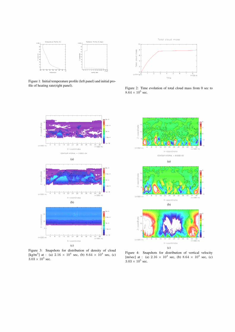
Figure 1: Initial temperature profile (left panel) and initial pro-file of heating rate(right panel).

(a)

(b)

(c)

Figure 3: Snapshots for distribution of density of cloud[kg/m3] at : (a) 2.16 × 104 sec, (b) 8.64 × 104 sec, (c)3.03 × 105 sec.

Figure 2: Time evolution of total cloud mass from 0 sec to8.64 × 105 sec.

(a)

(b)

(c)

Figure 4: Snapshots for distribution of vertical velocity[m/sec] at : (a) 2.16 × 104 sec, (b) 8.64 × 104 sec, (c)3.03 × 105 sec.