A process-based framework for quantifying the atmosphericpreconditioning of surface-triggered convection

Ahmed B. Tawfik1 and Paul A. Dirmeyer1

Received 12 September 2013; revised 11 November 2013; accepted 13 November 2013; published 9 January 2014.

[1] Here we introduce the heated condensation framework,which contains a suite of variables for isolating theatmospheric boundary state from local surface forcing. Thebuoyant condensation level (BCL) and buoyant mixingtemperature (θBM) quantify the degree to which the atmo-sphere is preconditioned for moist convection and can becalculated for any time of day or year using standard verticalprofiles of temperature and humidity. Unlike the liftedcondensation level and convective inhibition, the BCL isconstructed through incremental mixing from the surfacerather than lifting a hypothetical parcel. In this regard, theBCL represents a conserved condensation level diagnosticinherent to a given profile. The BCL and θBM are shown tobe applicable over a range of climate regimes and respond tosynoptic and mesoscale forcings, illustrating its broaderutility. A suite of variables relating the BCL directly tosurface fluxes is also introduced. Citation: Tawfik, A. B., andP. A. Dirmeyer (2014), A process-based framework for quantifyingthe atmospheric preconditioning of surface-triggered convection,Geophys. Res. Lett., 41, 173–178, doi:10.1002/2013GL057984.

1. Introduction

[2] The role of the land surface in triggering and amplify-ing precipitation has been the focus of recent research [e.g.,Zhang and Klein, 2010; Findell et al., 2011; Gentine et al.,2013b; Santanello et al., 2013] reflecting the ability of soilmoisture states to affect precipitation [Fennessy andShukla, 1999; Betts, 2004]. This coupling has been moststrongly identified over semiarid regions [Guo et al., 2006;Koster et al., 2006] due to greater flux sensitivity and vari-ability [Dirmeyer, 2011]. Thus, the potential exists forimproved seasonal predictability by better representation ofsoil moisture [Guo et al., 2011; Koster et al., 2011]. To betterunderstand the impact of surface forcing on precipitation,atmospheric preconditioning (the synoptic background state)must be quantified in a manner physically consistent withland-boundary layer interactions.[3] The growth of the planetary boundary layer (PBL)

throughout the day is a function of the interplay betweensurface fluxes, the vertical profile of the overlaying atmosphere,

and advection [Betts, 2000, 2009; Berg and Stull, 2004]. As thesurface is heated by incident radiation, near-surface airbecomes more buoyant. Rising air mixes upward, homoge-nizing the air within the growing PBL while entraining rel-atively dry air from the free troposphere [Berg and Stull,2004; Betts, 2009]. This results in near-constant potentialtemperature and water vapor mixing ratio profiles and alsoserves to define the PBL height itself. Clouds may form ifthe top of the PBL is sufficiently cooled [Gentine et al.,2013a; Zhang and Klein, 2013], potentially producing pre-cipitation [Haiden, 1997].[4] Treating land-atmosphere interactions as a cascade of

steps from the surface to the atmosphere allows the relativeimportance of different processes to be isolated [Seneviratneet al., 2010; Santanello et al., 2011]. Efforts have been madeto derive metrics for quantifying these particular steps [DeRidder, 1997; Findell and Eltahir, 2003; Ek and Holtslag,2004; Santanello et al., 2009; van Heerwaarden et al., 2010;Ferguson et al., 2012]. However, disentangling the large-scaleforcing from the local land surface forcing has been particu-larly difficult [Berg and Stull, 2004; Ferguson and Wood,2011]. Findell and Eltahir [2003] introduced a method usingmorning soundings that identifies certain regimes where theland surface may influence convective triggering. Althoughthis method was robust over Illinois, Ferguson and Wood[2011] had to modify thresholds to be suitable globally whenusing remote sensing data. Other studies have quantified thefree-tropospheric stability using temperature and specifichumidity lapse rates above the PBL within the context of con-vective triggering [De Ridder, 1997; Ek and Holtslag, 2004;Gentine et al., 2013b]. This is typically done using a “jump”criterion in a single-column model where conserved fields(potential temperature and specific humidity) are perturbed atthe top of the mixed layer mimicking the transition to the freetroposphere. Conserved parcel metrics such as the lifted con-densation level (LCL), the level of free convection (LFC),and convective inhibition (CIN) have also been used as diag-nostics for identifying convective triggering [Betts, 2004;Guichard et al., 2004; Zhang and Klein, 2010; Santanelloet al., 2011]. Santanello et al. [2011] showed that when theLCL is below the PBL depth, convection may occur providinga necessary but not sufficient condition for convective trigger-ing. Gentine et al. [2013b] used the difference between themixed layer and saturation equivalent potential temperatureabove the inversion to diagnose the difference between activeand forced convections.[5] These methods typically neglect the incremental growth

of the PBL by one of two assumptions: (1) basing metrics onatmospheric states at arbitrary heights or (2) lifting a parcelfrom a certain height without allowing the parcel to mix withits surroundings. This is problematic especially on hourlytimescales where LCL, LFC, and CIN are seen to vary

Additional supporting information may be found in the online version ofthis article.

1Center for Ocean-Land-Atmosphere Studies, GeorgeMason University,Fairfax, Virginia, USA.

Corresponding author: A. B. Tawfik, Center for Ocean-Land-AtmosphereStudies, George Mason University, 4400 University Drive, Mail Stop 6C5Fairfax, VA 22030, USA. (abtawfik@cola.iges.org)

©2013. American Geophysical Union. All Rights Reserved.0094-8276/14/10.1002/2013GL057984

173

GEOPHYSICAL RESEARCH LETTERS, VOL. 41, 173–178, doi:10.1002/2013GL057984, 2014

substantially throughout the day [Guichard et al., 2004;Betts, 2009], making it difficult for such metrics to identifya representative atmospheric background state with respectto convection.[6] Here we introduce a new diagnostic framework, the

heated condensation framework (HCF), which defines thebuoyant condensation level (BCL) and the buoyant mixingpotential temperature (θBM). These two variables quantifyhow conditioned the atmosphere is to moist free convectiondue to surface heating. The HCF variables are calculated usingstandard meteorological soundings (specific humidity andtemperature profiles) and may be calculated for any time ofday. The framework produces a suite of other quantities thatprovide insight into the conditions necessary for triggeringconvection, but the primary focus here will be on variables thatquantify the atmospheric background state (e.g., the BCL andθBM) with brief mention of how to calculate HCF variablesrelated to surface fluxes. These HCF surface flux variables willbe more thoroughly explored in a subsequent paper.

2. Heated Condensation Framework

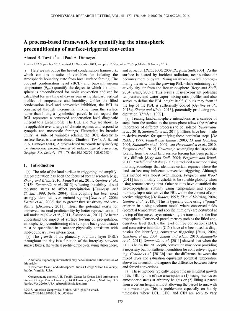
[7] The BCL is defined as the level at which saturationwould occur through buoyant mixing alone due to sensibleheating from the surface. Alternatively, the BCL is theheight the growing PBL needs to reach for saturation tooccur without the addition or removal of moisture fromthe column. To find the BCL, a hypothetical boundary layeris constructed using the vertical profiles of potential temper-ature, θ, and specific humidity, q. This is done in four stepsillustrated by the thermodynamic profiles in Figure 1: (1)Increase the near-surface potential temperature (θ2m) by asmall increment, Δθ (Figure 1a). (2) Find the height wherethe perturbed near-surface parcel (θ2m +Δθ) is neutrallybuoyant (Figure 1b). (3) Mix the specific humidity profilefrom the surface to the level of neutral buoyancy returninga constant mixed layer humidity, qmix (Figure 1b). (4)Upon mixing, check if saturation occurs at the top of thepotential mixed level (PML) by comparing qmix and thesaturation specific humidity at the PML, q*(θpml). The sequence

is repeated until saturation occurs (Figure 1c). Note that theBCL is a special case of the PML when saturation is reached(e.g., q*(θpml) � qmix = 0), where the sum of all Δθ incrementsrequired to attain the BCL is the total energy deficit, θdef(Figure 1c). Unlike parcel-derived metrics (LCL, LFC, convec-tive available potential energy, and CIN) that change for a givenprofile depending on the parcel selected for lifting, the BCL isan inherent property of a given profile that does not vary unlessthe temperature and humidity profiles change. This makes theBCL height independent from the initial θ2m and is thereforeinsensitive to the starting temperature (e.g., time of day) as longas the q and T profiles do not change.[8] Other useful quantities can also be derived within this

framework. Specifically, the buoyant mixing potential tem-perature, θBM, identifies the near-surface potential tempera-ture required to attain the BCL height (θBM= θ2m + θdef).Before the BCL height is reached (step 4; Figure 1b), a mois-ture deficit at the top of the potential mixed layer (PML) canbe calculated (qdef = q

*(θpml) � qmix). The θdef and qdef areboth easily translated into time integrated surface flux units.For example, multiplying qdef by the column density (ρh) ofthe potential mixed level returns the amount of moisture(either through evapotranspiration or advection) needed tobe injected into the PML for saturation to occur at a given po-tential temperature. Similarly, θdef multiplied by the specificheat capacity (cp) and mean column density (ρh) returns thenecessary sensible heat energy. Therefore, during each Δθincrement, the amount of heat input (cpρhΔθ) and moistureinput (ρhqdef) necessary for saturation can be quantified.

3. Data

3.1. Integrated Global Radiosonde Archive

[9] Vertical profiles of temperature and humidity are pro-vided by the Integrated Global Radiosonde Archive [IGRA;Durre et al., 2006]. The IGRA is a global quality-controlledsounding data set with the greatest spatial and temporal cov-erage over the United States and Europe typically measuringat 0000 UTC and 1200 UTC. Here we focus on the continen-tal United States (23–50°N and 130–66°W) with data from

a) b) c)

Figure 1. Thermodynamic profiles (e.g., skewT-logP diagrams) of temperature (black) and dew point temperature (blue)illustrating the steps for calculating the buoyant condensation level (BCL), buoyant mixing temperature (θBM), and mixedlayer specific humidity (qmix). Dashed green lines represent constant mixing ratio lines; dashed tan lines represent isotherms;and solid tan lines are dry adiabats. (a) The first step where θ2m is perturbed by some increment, Δθ. (b) The height, the po-tential mixed level (PML), where the perturbed surface parcel (θ2m +Δθ) is neutrally buoyant and the humidity profile ismixed from the PML to the surface. (c) The θ2m is perturbed until saturation occurs at the PML, and the level is identifiedas the BCL. The total potential temperature increment is θdef which is necessary to reach θBM from the initial θ2m. Faint blueand grey lines in Figure 1c refer to the unperturbed profile shown in Figure 1a as a reference.

TAWFIK AND DIRMEYER: HEATED CONDENSATION FRAMEWORK

174

January 1970 to June 2013 where available. To be used, eachsounding must have at least eight levels with 60% soundingsfor a station recordingmore than 20 levels. Additionally, sound-ings are filtered to include only those that reach 600 hPa toensure sufficient vertical resolution when calculating the HCFvariables. Finally, stations must have at least 500 soundings tobe included in the climatological analysis (section 4.2).

3.2. Rapid Refresh

[10] One week of output (23 July to 30 July 2012) from theRapid Refresh (RAP) forecast model system, the next gener-ation of the Rapid Update Cycle [Benjamin et al., 2004], isused to illustrate the utility of the HCF on hourly timescales.RAP is an operational short-range weather forecast systemusing the regional Weather Research and Forecast model(WRF-Advanced Research version 3.3) [Skamarock et al.,2008] to produce hourly forecasts over North America. TheRAPmodel has 50 vertical levels up to 10 hPa and a horizontalgrid spacing of 13 km. Here we use output from the first fore-cast hour providing a close representation of the assimilatedobservations. Instantaneous vertical profiles of temperature,specific humidity, and cloud cover are used, in addition to totalaccumulated precipitation over the prior hour.

4. Results

4.1. Event Application of HCF

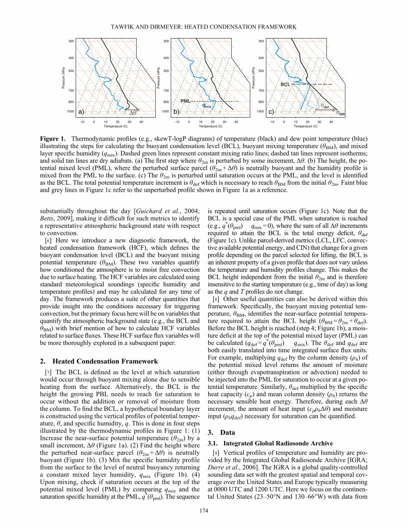
[11] A maritime (Miami, Florida) radiosonde station and acontinental (Amarillo, Texas) radiosonde station are examinedfor a week in July spanning days of year (DOY) 205–212(Figure 2). Miami and Amarillo are among the stations inFigure 3. The θ2m is compared against θBM instead of compar-ing the BCL and PBL heights to avoid uncertainties regardingdefinition and calculation of boundary layer height [Seidelet al., 2010; LeMone et al., 2013]. Note that the θBM-θ2m com-parison provides the same information regarding the departurefrom saturation as the BCL-PBL comparison except in a dif-ferent parameter space.[12] Although Miami and Amarillo represent two distinct

climate regimes, at both stations, precipitation and cloud coverare absent on days when daytime θBM is much larger than θ2m(Figure 2). Further, θBM calculated from RAP is shown toclosely follow θBM calculated from morning (1200 UTC)and afternoon (0000 UTC) IGRA observations, providingconfidence in the hourly RAP output (Figure 2). For Miami,θBM shows strong diurnal variations with a minimum of300K, typically during midmorning, and a maximum at night

Figure 2. Hourly buoyant mixing potential temperature, θBM, from RAP (black line) and IGRA soundings (black asterisk) com-pared against hourly 2m potential temperature fromRAP (blue line) and first sounding level potential temperature from IGRA (blueasterisk) from 23 July to 30 July 2012 for Miami, Florida (25.75°N and 80.83°W), and Amarillo, Texas (35.23°N and 101.70°W).RAP precipitation (green bars) is binned by hourly accumulations greater than 2mm and less than 2mm. Grey bars represent thepresence of nonprecipitating clouds lower than 8km above the ground also from RAP. Stations are identified in Figure 3.

TAWFIK AND DIRMEYER: HEATED CONDENSATION FRAMEWORK

175

greater than 310K. This suggests that there is a strong diurnalchange in low-level moisture consistent with a land-sea breeze(see supporting information for further discussion of theMiami land-sea breeze.) Convection appears to be controlledby the rapid daytime decrease of θBM (e.g., moistening ofthe large-scale background state and lowering BCL height)during this week.[13] At Amarillo, there is little diurnal variability in θBM,

suggesting that the atmospheric background state is not largelyinfluenced by local surface forcing during this week (Figure 2).Additionally, θBM rapidly increases during the evening ofDOY 209, during which time clear-sky conditions persist.This increase in θBM occurred when a ridge developed overthe central U.S. producing an upper level high-pressure systemcentered over northern Texas (see supporting informationfor further discussion.) However, there are times whenclouds and precipitation occur without a θBM-θ2m intersec-tion, namely at night for DOY 205–209. Because the HCFis developed to diagnose convective triggering due to surfaceheating, nocturnal precipitation events associated with eastwardpropagating mesoscale convective complexes [Moncrieff,2013] over the central U.S. likely would not influence θBMunless near-surface vertical profiles of q and θ were impacted.This is discussed further in section 5. Overall, we see theability of the HCF to capture the background atmosphericstate for nonprecipitating transient synoptic systems (Amarillohigh pressure system) and changes in mesoscale circulation(Miami land-sea breeze.)

4.2. BCL Height Climatology

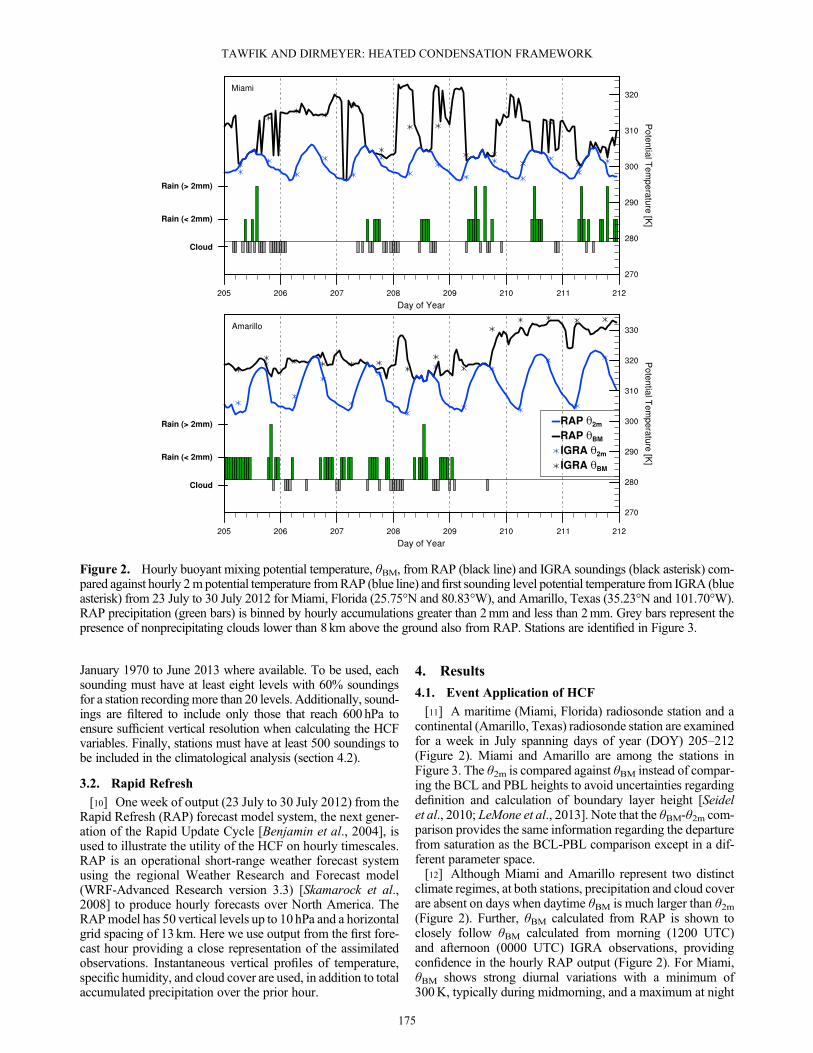
[14] The mean and standard deviations of the BCL heightare presented by season over the U.S., using several decadesof 1200 UTC IGRA data (Figure 3). The lowest BCL heightsoccur over the Southeastern U.S., and the highest values areover the Southwestern U.S. during the summer months

(June-July-August (JJA)) with a gradual transition from lowto high values moving westward. The seasonal cycle of aver-age BCL height is strongest in the southern half of the U.S.and east of the Rocky Mountains with a winter (December-January-February (DJF)) maximum between 3.8 and 5 kmand a summer (JJA) minimum of 1.5 and 3.5 km. This isexpected because convective activity typically peaks duringthe summer months. Conversely, the seasonal cycle for thenorthwest U.S. is weaker and has the lowest BCL heightsin DJF and highest in JJA. The Southwest shows almost noseasonal variation in BCL height (Figure 3).[15] The pattern of BCL height variability (σBCL) does not

change from fall (September-October-November) throughspring (March-April-May). However, there is a strong reduc-tion in variability that occurs during JJA from the SoutheastCoast through the Plains and Rocky Mountains (Figure 3).Furthermore, σBCL has the most pronounced seasonal cycleover the Southeast Coast with the BCL height varying bymore than 2.5 km from day-to-day in DJF and less than1.5 km in JJA.[16] Considering the seasonal behavior of BCL height, loca-

tions where the land surface may play a role in triggeringconvection can be deduced and highlighted for further investi-gation. Focusing on JJA, the BCL height patterns can bequalitatively separated into three categories: areas where theBCL height is (1) low, making convection likely under mostsurface (soil moisture) conditions, (2) attainable under specificsurface conditions making convection conditional on the landsurface state, and (3) so high as to make moist convectionunattainable. Note that these categories mirror the land-atmosphere regimes described by Findell and Eltahir [2003];however, the BCL height has the advantage of summarizingthe background state in a single metric without requiring theselection of arbitrary humidity or stability levels making theBCL height (or θBM) more globally applicable.

Figure 3. (left) Seasonal cycle of average buoyant condensation level (BCL in km), (middle) intraseasonal variability of theBCL (σBCL in km), and (right) average additional temperature increase necessary to trigger convection (θdef in K) at IGRAstations for 1200 UTC soundings. The stars represent the Amarillo, Texas, and Miami, Florida, stations.

TAWFIK AND DIRMEYER: HEATED CONDENSATION FRAMEWORK

176

[17] To provide an examination of the likelihood of convec-tive triggering, the average θdef is also presented (Figure 3),where smaller values represent a greater chance of triggering.The seasonal cycle is amplified when presented in termsof θdef, with DJF requiring an increase of more than 28K fromthe morning θ2m (1200 UTC) on average for most of the U.S.and less than 18K for JJA (Figure 3). As a first approximationfor identifying the three regimes, terciles of the average θdefacross all stations and seasons were calculated, where valuesless than 16K (~33rd percentile) represent the first regime,values between 16 and 23K represent the second regime,and values greater than 23K (~67th percentile) represent thethird. The Southeast and Gulf Coasts would likely fall underthe first regime because an increase in surface potential tem-perature of less than 16K is required on average to triggerconvection for JJA. The West Coast would lie in the thirdregime (convection unattainable over any surface) becausemorning (1200 UTC) θ2m would need to increase by morethan 23K to trigger convection. The Central Plains, typicallyidentified as a land-atmosphere coupling hotspot [Kosteret al., 2006], and the Great Lakes region fall into the secondregime, suggesting that convection may be favored if thereis a sustained moisture source (through low-level moistureconvergence or evapotranspiration) into the PBL or the surfaceis sufficiently dry, making it capable of overcoming the 16–23K temperature deficit (Figure 3). Station-specific parame-ters that influence the diurnal temperature range (such as veg-etation type, soil moisture, and soil properties) could influencethe boundary between the three regimes. To more rigorouslycategorize these regimes, the diurnal evolution of θdef mustbe examined. However, IGRA observations do not providesufficient hourly resolution to perform this analysis.

5. Discussion and Conclusions

[18] A process-based diagnostic framework (HCF) is intro-duced to quantify the atmospheric background state within thecontext of land-boundary layer interactions. The HCF has ad-vantages that make it useful for studying the impact of surfacefluxes on convective triggering. First, the construction of theBCL height mimics the evolution of the convective boundarylayer and initiation of convection to first order (Figure 1).Rather than lifting a hypothetical unmixed parcel, the HCFconstructs a hypothetical boundary layer by incrementally in-putting heat at the surface. Information regarding the atmo-spheric background state (via BCL height and θBM) andsurface energy interaction can be derived (using θdef and qdef)that are physically consistent with PBL development. TheBCL height and θBM are diagnostic properties of a given pro-file not subject to parcel selection bias. The BCL is similar tothe mixing condensation level (MCL), which has long beenused for examining fog [Petterssen, 1939] and marine strato-cumulus [Miller et al., 1998]. The primary difference is thatthe MCL assumes wind-driven mixing of both the θ and qprofiles, whereas the BCL assumes buoyancy-driven mixingby perturbing θ2m and mixing the q profile. An analogy couldalso be drawn with the convective condensation level (CCL);however, like the LCL, the CCL is calculated by lifting a par-cel of water vapor that does not mix with its surroundings,resulting in the same shortcomings discussed above.[19] Another advantage is that an atmospheric background

state can be calculated during any time of day (Figure 2) or year(Figure 3). This allows for the evaluation of land-atmosphere

coupling on an hourly basis without having to remove weathervariability by time-averaging [cf., Betts, 2004;Guo et al., 2006;Koster et al., 2006]. The HCF may be easily applied becauseonly temperature and humidity profiles are required. The sensi-tivity of the HCF to vertical resolution needs to be examinedfurther; however, preliminary analysis shows that mean BCLheight changes by less than +/�500m for 75% of 1200 UTCsoundings when the number of IGRA vertical levels are halved.Additionally, when analyzing 1200 UTC soundings BCLheight climatology (Figure 3), the difference in solar timeacross the U.S. introduces biases of less than 160 m for moststations when using hourly RAP output from July 2012.[20] Similar to other column-derived metrics [De Ridder,

1997; Findell and Eltahir, 2003], a primary shortcoming ofHCF is its inability to distinguish between transient andlocally driven precipitation. Although it was shown to cap-ture low-level moisture advection (Figure 2), a passing pre-cipitation event may rapidly lower the BCL height throughreevaporation of precipitation within the PBL. This makesthe signal between reevaporation and rapid low-level mois-ture convergence difficult to determine without subhourlyprofiles or information of surrounding synoptic conditions.Therefore, although the evolution of the atmospheric back-ground state is accurately captured, more information wouldbe required to identify the specific process. Combining BCLinformation with existing coupling diagnostics, such as theLCL deficit representation of near-surface parcel forcing[Santanello et al., 2011], may help identify the role of theland surface in triggering and enhancing convection.

[21] Acknowledgments. This work was supported by National ScienceFoundation grant 0947837 for Earth System Modeling post-docs. We wouldlike to thank Bert Holtslag, Kirsten Findell, Craig Ferguson, Chiel vanHeerwaarden, Alan Betts, Pierre Gentine, Randal Koster, Joseph Santanello,and Michael Ek for their helpful comments that have truly improved the qual-ity of this manuscript.[22] The Editor thanks Craig Ferguson and an anonymous reviewer for

assistance evaluating this manuscript.

ReferencesBenjamin, S. G., et al. (2004), An hourly assimilation forecast cycle: TheRUC, Mon. Weather Rev., 132, 495, doi:10.1175/1520-0493(2004)132<0495:AHACTR>2.0.CO;2.

Berg, L. K., and R. B. Stull (2004), Parameterization of joint frequency dis-tributions of potential temperature and water vapor mixing ratio in thedaytime convective boundary layer, J. Atmos. Sci., 61(7), 813–828,doi:10.1175/1520-0469(2004)061<0813:POJFDO>2.0.CO;2.

Betts, A. K. (2000), Idealized model for equilibrium boundary layer overland, J. Hydrometeorol., 1(6), 507–523, doi:10.1175/1525-7541(2000)001<0507:IMFEBL>2.0.CO;2.

Betts, A. K. (2004), Understanding hydrometeorology using global models,Bull.Am. Meteorol. Soc., 85(11), 1673–1688, doi:10.1175/BAMS-85-11-1673.

Betts, A. K. (2009), Land-surface-atmosphere coupling in observations andmodels, J. Adv. Model. Earth Syst., 2, doi:10.3894/JAMES.2009.1.4. [on-line] Available from: http://james.agu.org/index.php/JAMES/article/view/v1n4 (Accessed 13 September 2012)

De Ridder, K. (1997), Land surface processes and the potential for convectiveprecipitation, J. Geophys. Res., 102(D25), 30,085–30,090, doi:10.1029/97JD02624.

Dirmeyer, P. A. (2011), The terrestrial segment of soil moisture-climate cou-pling, Geophys. Res. Lett., 38, L16702, doi:10.1029/2011GL048268.

Durre, I., R. S. Vose, and D. B. Wuertz (2006), Overview of the IntegratedGlobal Radiosonde Archive, J. Clim., 19(1), 53–68, doi:10.1175/JCLI3594.1.

Ek, M. B., and A. A. M. Holtslag (2004), Influence of soil moisture onboundary layer cloud development, J. Hydrometeorol., 5(1), 86–99,doi:10.1175/1525-7541(2004)005<0086:IOSMOB>2.0.CO;2.

Fennessy, M. J., and J. Shukla (1999), Impact of initial soil wetness on sea-sonal atmospheric prediction, J. Clim., 12(11), 3167–3180, doi:10.1175/1520-0442(1999)012<3167:IOISWO>2.0.CO;2.

TAWFIK AND DIRMEYER: HEATED CONDENSATION FRAMEWORK

177

Ferguson, C. R., and E. F. Wood (2011), Observed land-atmosphere cou-pling from satellite remote sensing and reanalysis, J. Hydrometeorol.,12(6), 1221–1254, doi:10.1175/2011JHM1380.1.

Ferguson, C. R., E. F. Wood, and R. K. Vinukollu (2012), A globalintercomparison of modeled and observed land-atmosphere coupling,J. Hydrometeorol., 13(3), 749–784, doi:10.1175/JHM-D-11-0119.1.

Findell, K. L., and E. A. B. Eltahir (2003), Atmospheric controls on soilmoisture-boundary layer interactions. Part I: Framework development,J. Hydrometeorol., 4(3), 552–569, doi:10.1175/1525-7541(2003)004<0552:ACOSML>2.0.CO;2.

Findell, K. L., P. Gentine, B. R. Lintner, and C. Kerr (2011), Probability ofafternoon precipitation in eastern United States and Mexico enhanced byhigh evaporation, Nat. Geosci., 4(7), 434–439, doi:10.1038/ngeo1174.

Gentine, P., A. K. Betts, B. R. Lintner, K. L. Findell, C. C. van Heerwaarden,and F. D’Andrea (2013a), A probabilistic bulk model of coupled mixedlayer and convection. Part II: Shallow convection case, J. Atmos. Sci.,70(6), 1557–1576, doi:10.1175/JAS-D-12-0146.1.

Gentine, P., A. A. M. Holtslag, F. D’Andrea, and M. Ek (2013b), Surfaceand atmospheric controls on the onset of moist convection over land,J. Hydrometeorol., 14, 1443–1462, doi:10.1175/JHM-D-12-0137.1.

Guichard, F., et al. (2004), Modelling the diurnal cycle of deep precipitatingconvection over landwith cloud-resolvingmodels and single-columnmodels,Q. J. R. Meteorol. Soc., 130(604), 3139–3172, doi:10.1256/qj.03.145.

Guo, Z., et al. (2006), GLACE: The global land-atmosphere coupling exper-iment. Part II: Analysis, J. Hydrometeorol., 7(4), 611–625, doi:10.1175/JHM511.1.

Guo, Z., P. A. Dirmeyer, and T. DelSole (2011), Land surface impacts onsubseasonal and seasonal predictability, Geophys. Res. Lett., 38, L24812,doi:10.1029/2011GL049945.

Haiden, T. (1997), An analytical study of cumulus onset, Q. J. R. Meteorol.Soc., 123(543), 1945–1960, doi:10.1002/qj.49712354309.

Koster, R. D., et al. (2006), GLACE: The global land-atmosphere couplingexperiment. Part I: Overview, J. Hydrometeorol., 7(4), 590–610,doi:10.1175/JHM510.1.

Koster, R. D., et al. (2011), The second phase of the global land-atmospherecoupling experiment: Soil moisture contributions to subseasonal forecastskill, J. Hydrometeorol., 12(5), 805–822, doi:10.1175/2011JHM1365.1.

LeMone, M. A., M. Tewari, F. Chen, and J. Dudhia (2013), Objectively de-termined fair-weather CBL depths in the ARW-WRF model and theircomparison to CASES-97 observations, Mon. Weather Rev., 141(1),30–54, doi:10.1175/MWR-D-12-00106.1.

Miller, M. A., M. P. Jensen, and E. E. Clothiaux (1998), Diurnal cloud andthermodynamic variations in the stratocumulus transition regime: A case

study using in situ and remote sensors, J. Atmos. Sci., 55(13), 2294–2310,doi:10.1175/1520-0469(1998)055<2294:DCATVI>2.0.CO;2.

Moncrieff,M.W. (2013), Themultiscale organization of moist convection andthe intersection of weather and climate, in Climate Dynamics: Why DoesClimate Vary?, edited by D.-Z. Sun and F. Bryan, pp. 3–26, AGU,Washington D. C., doi:10.1029/2008GM000838.

Petterssen, S. (1939), Some aspects of formation and dissipation of fog,Geofys. Publ., 12(10), 22.

Santanello, J. A., C. D. Peters-Lidard, S. V. Kumar, C. Alonge, andW.-K. Tao(2009), A modeling and observational framework for diagnosing local land-atmosphere coupling on diurnal time scales, J. Hydrometeorol., 10(3),577–599, doi:10.1175/2009JHM1066.1.

Santanello, J. A., C. D. Peters-Lidard, and S. V. Kumar (2011), Diagnosing thesensitivity of local land-atmosphere coupling via the soil moisture-boundarylayer interaction, J. Hydrometeorol., 12(5), 766–786, doi:10.1175/JHM-D-10-05014.1.

Santanello, J. A., C. D. Peters-Lidard, A. Kennedy, and S. V. Kumar (2013),Diagnosing the nature of land-atmosphere coupling: A case study of dry/wet extremes in the U.S. Southern Great Plains, J. Hydrometeorol., 14(1),3–24, doi:10.1175/JHM-D-12-023.1.

Seidel, D. J., C. O. Ao, and K. Li (2010), Estimating climatological planetaryboundary layer heights from radiosonde observations: Comparison ofmethods and uncertainty analysis, J. Geophys. Res., 115, D16113,doi:10.1029/2009JD013680.

Seneviratne, S. I., T. Corti, E. L. Davin, M. Hirschi, E. B. Jaeger, I. Lehner,B. Orlowsky, and A. J. Teuling (2010), Investigating soil moisture-climateinteractions in a changing climate: A review, Earth Sci. Rev., 99(3–4),125–161, doi:10.1016/j.earscirev.2010.02.004.

Skamarock,W. C., J. B. Klemp, J. Dudhia, D. O. Gill, D.M. Barker,M.G.Duda,X.-Y. Huang, W. Wang, and J. G. Powers (2008), A description of theadvanced research WRF version 3, NCAR Tech. Note, NCAR/TN–475+STR.

Van Heerwaarden, C. C., J. Vilà-Guerau deArellano, A. Gounou, F. Guichard,and F. Couvreux (2010), Understanding the daily cycle of evapotranspira-tion: A method to quantify the influence of forcings and feedbacks,J. Hydrometeorol., 11(6), 1405–1422, doi:10.1175/2010JHM1272.1.

Zhang, Y., and S. A. Klein (2010), Mechanisms affecting the transition fromshallow to deep convection over land: Inferences from observations of thediurnal cycle collected at the ARM Southern Great Plains site, J. Atmos.Sci., 67(9), 2943–2959, doi:10.1175/2010JAS3366.1.

Zhang, Y., and S. A. Klein (2013), Factors controlling the vertical extent offair-weather shallow cumulus clouds over land: Investigation of diurnal-cycle observations collected at the ARM Southern Great Plains Site,J. Atmos. Sci., 70(4), 1297–1315, doi:10.1175/JAS-D-12-0131.1.

TAWFIK AND DIRMEYER: HEATED CONDENSATION FRAMEWORK

178