Embed Size (px)
Citation preview
International Journal of Mathematical, Engineering and Management Sciences
Vol. 6, No. 2, 493-509, 2021
https://doi.org/10.33889/IJMEMS.2021.6.2.030
493
Atangana-Baleanu and Caputo-Fabrizio Analysis of Fractional
Derivatives on MHD Flow past a Moving Vertical Plate with Variable
Viscosity and Thermal Conductivity in a Porous Medium
Dipen Saikia
Department of Basic and Applied Science,
National Institute of Technology Arunachal Pradesh, Yupia, Arunachal Pradesh, India.
E-mail: [email protected]
Utpal Kumar Saha Department of Basic and Applied Science,
National Institute of Technology Arunachal Pradesh, Yupia, Arunachal Pradesh, India.
Corresponding author: [email protected]
Gopal Chandra Hazarika Department of Mathematics,
Dibrugarh University, Dibrugarh, Assam, India.
E-mail: [email protected]
(Received April 6, 2020; Accepted September 8, 2020)
Abstract
In this paper, a numerical investigation is presented for non-integer order derivatives with Atangana-Baleanu (AB) and
Caputo-Fabrizio (CF) fractional derivatives for the variable viscosity and thermal conductivity over a moving vertical
plate in a porous medium two dimensional free convection unsteady MHD flow. The effects of radiation have also been
considered. The governing partial differential equations along with the boundary conditions are changed to ordinary
form by similarity transformations. Hence physical parameters show up in the equations and interpretations on these
parameters can be achieved suitably.By using ordinary finite difference scheme the equations are discritized and
developed in fractional form. These discritized equations are numerically solved by the approach based on Gauss-seidel
iteration scheme. Some numerical strategies are used to find the values of AB and CF approaches on time by
developing programming code in MATLAB. The effects of all the physical parameters involved in the problem on
velocity, temperature and concentration distribution are compared graphically as well as in tabular form. The effects of
each parameter are found to be prominent. We have observed a significant variation of values under different
parameters using AB and CF approaches on velocity, temperature and concentration distribution with respect to time.
Keywords- AB and CF derivatives, Viscosity, Thermal conductivity, Porous medium, Radiation.
1. Introduction The boundary layer and heat transfer flow of a viscous fluid over a moving vertical plate in a
porous medium have been investigated in a number of technological approaches such as warm
rolling, metallic extrusion, petroleum industries, polymer extrusion, wires drawing
and metallic spinning. Natural convection flows driven by temperature differences are of great
interest in a number of industrial applications. Bejan and Khair (1985) studied free convection
heat and mass transfer in a porous medium. In recent there has been a growing interest in studing
the combined application of MHD flow and porous media. Aldoss et al. (1995) investigated
combined free and forced convection flow from vertical plate in aporous medium in the presence
of magnetic field. Hossain and Munir (2000) analysed a two dimensional mixed convection flow
of a viscous incompressible fluid of temperature dependent viscosity past a vertical plate.
International Journal of Mathematical, Engineering and Management Sciences
Vol. 6, No. 2, 493-509, 2021
https://doi.org/10.33889/IJMEMS.2021.6.2.030
494
Javaherdeh et al. (2015) studied the natural convection heat and mass transfer in MHD fluid flow
past a moving vertical plate with variable surface temperature and concentration in a porous
medium. However, the impact of variable viscosity and thermal conductivity of a MHD free
convection flow past a vertical plate embedded in porous medium has received a little attention.
Mukhopadhyay and Layek (2008) presented the effects of variable viscosity through a porous
medium over a stretching sheet in presence of thermal radiation.
Recently, fractional calculus has gained tremendous popularity among the researchers because of
singular kernel with locality and non-singular kernel with non-locality problem. Caputo and
Fabrizio used an exponential function in fractional derivative to avoid the singular kernel
problem. Mirza and Vieru (2017) analyzed that the use of the time-fractional derivative without
singular kernel is more advantageous than Caputo time-fractional derivative. Nehad et al. (2016)
applied CF fractional derivatives to analyze the solutions for heat transfer of second grade fluids
over vertical oscillating plates. “A comparative study has been obtained by using the AB and CF
fractional derivatives for casson fluid model with chemical reaction and heat generation” by
Sheikh et al. (2017). Few works using fractional derivatives have been studied in Histrov (2017),
Atangana and Baleanu (2016). A comparative study of Atangana-Baleanu and Caputo-Fabrizio
evaluation of fractional derivatives for heat and mass transfer of fluid over a vertical plate has
been done by Khan et al. (2017).
The main objective of this paper is to investigate the effects of variable viscosity and thermal
conductivity over a moving vertical plate in porous medium and comparing the results with the
approaches AB and CF fractional derivatives. The non-dimensional governing equations with the
non-dimensional boundary conditions are discretized with ordinary finite-difference kernel solved
numerically with the help of AB and CF fractional derivative methods by developing suitable
programming code in MATLAB. A comparative analysis under different parameters is
represented graphically as well as in tabular form.
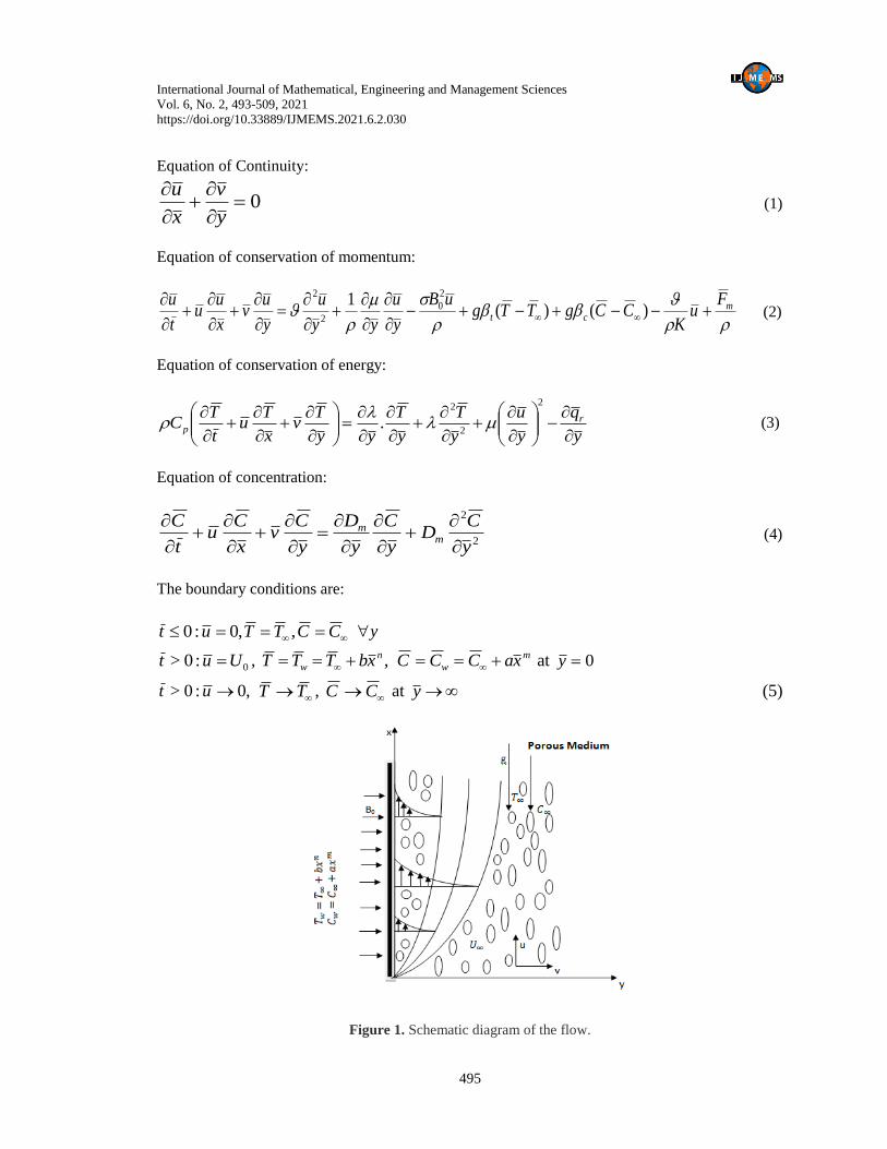
2. Mathematical Formulation Consider a two-dimensional free convection steady heat and mass transfer flow of viscous
incompressible electrically conducting fluid past a moving vertical plate in a porous medium
(Figure 1). Here a uniform magnetic field is applied in a direction perpendicular to the fluid flow.
The x - axis is taken along the vertical plate in the direction of the flow and y axis is normal to
it. At 0t , the fluid have gained the temperature wT , and concentration level near the plate is
wC . The fluid properties are assumed to be constant except for the fluid viscosity and thermal
conductivity which are assumed to vary as an inverse linear function of temperature. A uniform
magnetic field of strength 0B is applied normal to the plate. There is no chemical reaction
between the fluid and diffusing species. Plate temperature wT is variable and T is the free
stream temperature assumed constant.
The variable viscosity and thermal conductivity are governed by the following equations under
the boundary layer approximation:
International Journal of Mathematical, Engineering and Management Sciences
Vol. 6, No. 2, 493-509, 2021
https://doi.org/10.33889/IJMEMS.2021.6.2.030
495
Equation of Continuity:
0
y
v
x
u (1)
Equation of conservation of momentum:
m
ct
Fu
KCCgTTg
uB
y
u
yy
u
y
uv
x
uu
t
u
)()(
12
0
2
2
(2)
Equation of conservation of energy:
y
q
y
u
y
T
y
T
yy
Tv
x
Tu
t
TC r
p
2
2
2
.
(3)
Equation of concentration:
2
2
y
CD
y
C
y
D
y
Cv
x
Cu
t
Cm
m
(4)
The boundary conditions are:
CCTTut ,,0:0 y
0:0> Uut , ,n
w xbTTT m
w xaCCC at 0y
,0:0> ut TT , CC at y (5)
Figure 1. Schematic diagram of the flow.
International Journal of Mathematical, Engineering and Management Sciences
Vol. 6, No. 2, 493-509, 2021
https://doi.org/10.33889/IJMEMS.2021.6.2.030
496
where, u and v are the fluid velocities in the direction of x and y respectively, is the
kinematic viscosity, is the kinematic viscosity of the fluid in the free stream, is the fluid
density, is the viscosity of the fluid, is the electrical conductivity, g is the acceleration due
to gravity, t is the volume expansion coefficient for heat transfer, c is the volume expansion
coefficient for mass transfer, T is the fluid temperature within the boundary layer,T is the
temperature at free stream of the fluid, C is the species concentration of the fluid,C is the
concentration at free stream of the fluid, is the thermal conductivity of the fluid, pC is the
specific heat at constant pressure, rq is the radiative heat flux, mD is the mass diffusivity, 0U is
the velocity of the plate, K is permeability of the porous medium, J is the electric current
density, a is the mean absorption coefficient, is the Stefan – Boltzmann constant.
where, 2
0BuBBqBJFm
, q
be fluid velocity at a particular point, jBB
0
be the applied magnetic field.
By Rosseland approximation,
The radiative heat flux, y
T
aqr
4
3
4 (6)
We expand 4T in Taylor’s series about T as follows:
...........)(6)(4 22344 TTTTTTTT
By neglecting the higher order terms beyond 1st degree in TT we have
434 34 TTTT (7)
Using equations (6) and (7), equation (3) reduces to
2
4232
2
2
3
16.
y
T
a
T
y
u
y
T
y
T
yy
Tv
x
Tu
t
TCp
(8)
Appling the following non dimensional quantities:
,0
xUx ,0
yUy ,
0U
uu ,
0U
vv
TT
TT
w
w ,
CC
CC
w
w ,
tUt
2
0
(9)
According to Lai and Kulacki (1990) the viscosity and thermal conductivity of the fluid are
assumed to be inverse linear function of temperature as follows:
International Journal of Mathematical, Engineering and Management Sciences
Vol. 6, No. 2, 493-509, 2021
https://doi.org/10.33889/IJMEMS.2021.6.2.030
497
TT
111
(10)
TT
111
(11)
where, and are constants which depend on the thermal property of the fluid.
We define two parameters as,
TT
TT
w
rwr is called viscosity parameter and
TT
TT
w
cwc
is
called thermal Conductivity parameter.
Using these two parameters in (10) and (11), we have the viscosity and thermal conductivity
respectively as
r
r
)1(
, c
c
)1(
(12)
It is also important to note that r is negative for liquid and positive for gases.
Using the transformations (9) and (12), the non-dimensional forms of (2), (3) and (4) are
y
u
yy
u
y
uv
x
uu
t
u
r
r
r
r
22
2 11
p
r
rm uKGrGrMu
1)1()1( (13)
22
22
2
.Pr111
3
4)1(Pr
y
uEc
yyK
yvu
x
n
xu
t r
r
r
r
c
c
r
(14)
2
2
2
11.
1.
1)1(
yScyyScyvu
x
m
xu
t c
c
r
r
(15)
The corresponding initial and boundary conditions are transformed to:
,0:0 ut ,0v ,0 0 y
,1:0> ut ,0v ,0 0 at 0y
,0:0> ut 0v , 1 , 1 at y (16)
International Journal of Mathematical, Engineering and Management Sciences
Vol. 6, No. 2, 493-509, 2021
https://doi.org/10.33889/IJMEMS.2021.6.2.030
498
where,pw
o
CR
UEc
2
is the Eckert number, 2
0
2
KU
uK p
is the Permeability parameter,
mDSc
is the Schmidt number,
2
0
2
0
U
BM
is the Magnetic field
parameter,2
0
2
3
16
U
TaKr
is the radiation parameter,
3
0U
TTgGr wt
is the Grashof
Number,
3
0U
CCgGr wc
m
is the Concentration buoyancy parameter and
pCPr is
the Prandlt number.
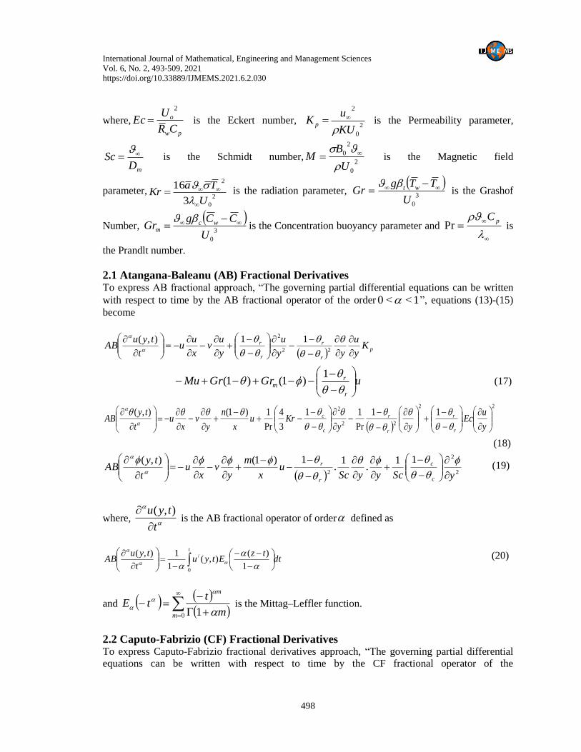
2.1 Atangana-Baleanu (AB) Fractional Derivatives To express AB fractional approach, “The governing partial differential equations can be written
with respect to time by the AB fractional operator of the order 1<<0 ”, equations (13)-(15)
become
p
r
r
r
r Ky
u
yy
u
y
uv
x
uu
t
tyuAB
22
2 11),(
uGrGrMur
rm
1)1()1( (17)
22
22
2
.11
Pr
11
3
4
Pr
1)1(),(
y
uEc
yyKru
x
n
yv
xu
t
tyAB
r
r
r
r
c
c
(18)
2
2
2
11.
1.
1)1(
),(
yScyyScu
x
m
yv
xu
t
tyAB
c
c
r
r
(19)
where,
t
tyu
),( is the AB fractional operator of order defined as
dttz
Etyut
tyuAB
t
0
/
1
)(),(
1
1),(
(20)
and
0 1m
m
m
ttE
is the Mittag–Leffler function.
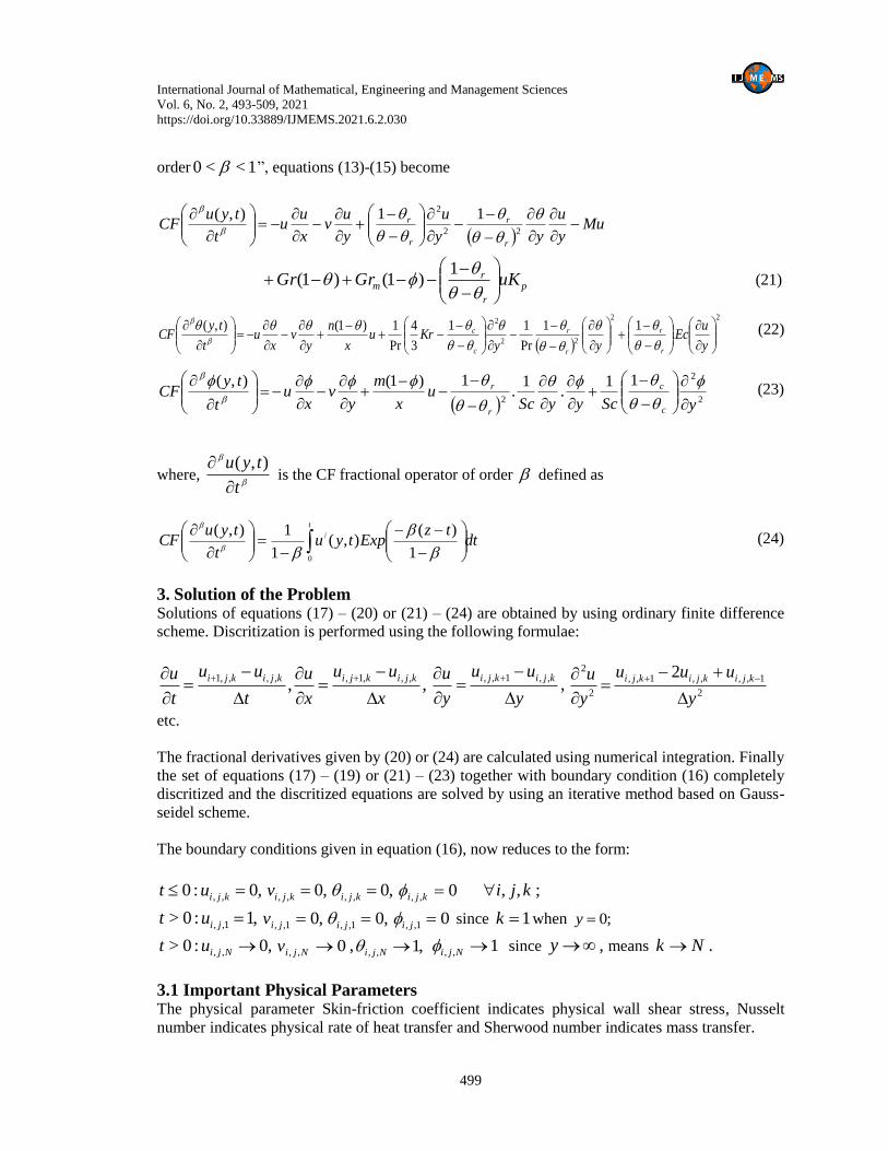
2.2 Caputo-Fabrizio (CF) Fractional Derivatives To express Caputo-Fabrizio fractional derivatives approach, “The governing partial differential
equations can be written with respect to time by the CF fractional operator of the
International Journal of Mathematical, Engineering and Management Sciences
Vol. 6, No. 2, 493-509, 2021
https://doi.org/10.33889/IJMEMS.2021.6.2.030
499
order 1<<0 ”, equations (13)-(15) become
Mu
y
u
yy
u
y
uv
x
uu
t
tyuCF
r
r
r
r
22
2 11),(
p
r
rm uKGrGr
1)1()1( (21)
22
22
2
.11
Pr
11
3
4
Pr
1)1(),(
y
uEc
yyKru
x
n
yv
xu
t
tyCF
r
r
r
r
c
c
(22)
2
2
2
11.
1.
1)1(
),(
yScyyScu
x
m
yv
xu
t
tyCF
c
c
r
r
(23)
where,
t
tyu
),( is the CF fractional operator of order defined as
dttz
Exptyut
tyuCF
t
0
/
1
)(),(
1
1),(
(24)
3. Solution of the Problem
Solutions of equations (17) – (20) or (21) – (24) are obtained by using ordinary finite difference
scheme. Discritization is performed using the following formulae:
,,,,,1,,,,,1
x
uu
x
u
t
uu
t
u kjikjikjikji
,
,,1,,
y
uu
y
u kjikji
2
1,,,,1,,
2
2 2
y
uuu
y
u kjikjikji
etc.
The fractional derivatives given by (20) or (24) are calculated using numerical integration. Finally
the set of equations (17) – (19) or (21) – (23) together with boundary condition (16) completely
discritized and the discritized equations are solved by using an iterative method based on Gauss-
seidel scheme.
The boundary conditions given in equation (16), now reduces to the form:
,0:0 ,, kjiut ,0,, kjiv ,0,, kji 0,, kji kji ,, ;
,1:0> 1,, jiut ,01,, jiv ,01,, ji 01,, ji since 1k when 0;y
,0:0> ,, Njiut 0,, Njiv , ,1,, Nji 1,, Nji since y , means Nk .
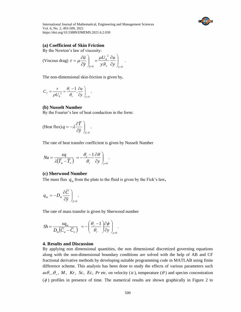
3.1 Important Physical Parameters The physical parameter Skin-friction coefficient indicates physical wall shear stress, Nusselt
number indicates physical rate of heat transfer and Sherwood number indicates mass transfer.
International Journal of Mathematical, Engineering and Management Sciences
Vol. 6, No. 2, 493-509, 2021
https://doi.org/10.33889/IJMEMS.2021.6.2.030
500
(a) Coefficient of Skin Friction By the Newton’s law of viscosity:
(Viscous drag)
0
yy
u
0
2
0
yy
u
y
U
.
The non-dimensional skin-friction is given by,
2
0 0
1.r
f
r y
uC
U y
.
(b) Nusselt Number By the Fourier’s law of heat conduction in the form:
(Heat flux)
0
yy
Tq .
The rate of heat transfer coefficient is given by Nusselt Number
TT
xqNu
w
0
1
yc
c
y
.
(c) Sherwood Number
The mass flux mq from the plate to the fluid is given by the Fick’s law,
0
y
mmy
CDq .
The rate of mass transfer is given by Sherwood number
CCD
xqSh
wm
m
0
1
yr
r
y
.
4. Results and Discussion By applying non dimensional quantities, the non dimensional discretized governing equations
along with the non-dimensional boundary conditions are solved with the help of AB and CF
fractional derivative methods by developing suitable programming code in MATLAB using finite
difference scheme. This analysis has been done to study the effects of various parameters such
as r , c , ,M ,Kr ,Sc ,Ec Pr etc. on velocity ( u ), temperature ( ) and species concentration
( ) profiles in presence of time. The numerical results are shown graphically in Figure 2 to
International Journal of Mathematical, Engineering and Management Sciences
Vol. 6, No. 2, 493-509, 2021
https://doi.org/10.33889/IJMEMS.2021.6.2.030
501
Figure 15. In the following discussion, the initial values of the parameters are considered as
20,r 12, 1, 0.25, 0.1, 0.1, 0.25, 0.05, 0.5, 0.1, Pr 0.25, 0.5c m pM Gr Gr Kr Sc Ec K
unless otherwise stated.
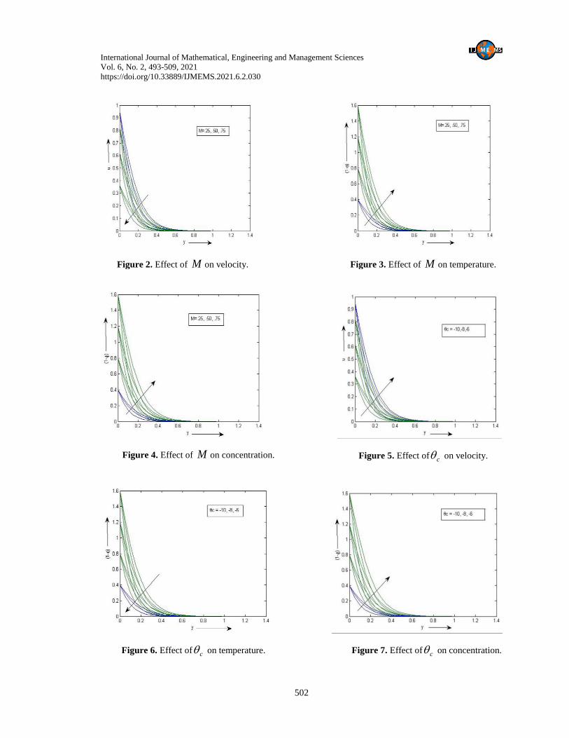
4.1 Graphical Representation In Figure 2, it is seen that with the increasing value of the Hartmann number, velocity decreases.
The presence of magnetic field in the normal direction of the flow in an electrically conducting
fluid produces Lorentz force which opposes the flow. To overcome this opposing force, some
extra work should be done which is transformed to heat energy. Hence temperature increases
(Figure 3). This is because that the applied magnetic field opposes the fluid motion and therefore
enhancing the temperature for this response. With the increase of M species concentration also
increases (Figure 4).
Figure 5 depicts the distribution of velocity with the variation of the thermal conductivity
parameter c . Velocity increases with the increasing value of c . In Figure 6 temperature
decreases with the increasing value of c . Physically it means that as thermal conduction
increases the transportation of heat from hot region to colder region increases. Since temperature
within boundary layer is more than the outside so temperature is decreased. Again species
concentration increases with the increasing value of c (Figure 7).
The effects of viscosity parameter r on velocity, temperature and species concentration
distribution are plotted in Figure 8 to Figure 10. Figure 8 displays that dimensionless velocity
decreases with the increase of r . This is due to the fact that with the increase of the viscosity
parameter the thickness of the velocity boundary layer decreases. Physically, this is because of
that a larger r implies higher temperature difference between the fluid and the surface. Figure 9
shows that temperature increases with the increasing value of r . The viscosity causes a rise in
the friction, when friction increases the area of the stretching surface in contact with the flow
increases therefore generated heat from the friction on the surface is transferred to the flow which
leads to a rise in the surface temperature and the flow is heated. The species concentration
decreases for increasing value of r (Figure 10).
The Eckert number Ec signifies the viscous dissipation of the fluid, on temperature it is plotted in
Figure 11. It is seen that an increase in viscous dissipation of the fluid tends to increase in fluid
temperature with increase of Ec. In Figure 12, it is noticed that with the increase of radiation
parameter Kr temperature increases. This is due to the fact that the thermal boundary layer
thickness increases with the increase of Kr and hence temperature. Velocity decreases with the
increasing value of Prandtl number Pr (Figure 13). This is due to the fact that with the increase of
Pr, viscosity increases, so velocity decreases. In Figure 14, it is noticed that with the increasing
value of Pr temperature of the fluid decreases. For higher Prandtl number the fluid has a
relatively high thermal conductivity which decreases the temperature.
International Journal of Mathematical, Engineering and Management Sciences
Vol. 6, No. 2, 493-509, 2021
https://doi.org/10.33889/IJMEMS.2021.6.2.030
502
Figure 2. Effect of M on velocity. Figure 3. Effect of M on temperature.
Figure 4. Effect of M on concentration. Figure 5. Effect of c on velocity.
Figure 6. Effect of c on temperature. Figure 7. Effect of c on concentration.

International Journal of Mathematical, Engineering and Management Sciences
Vol. 6, No. 2, 493-509, 2021
https://doi.org/10.33889/IJMEMS.2021.6.2.030
503
Figure 8. Effect of r on velocity Figure 9. Effect of r on temperature.
Figure 10. Effect of r on concentration. Figure 11. Effect of Ec on temperature.
Figure 12. Effect of Kr on temperature. Figure 13. Effect of Pr on velocity.

International Journal of Mathematical, Engineering and Management Sciences
Vol. 6, No. 2, 493-509, 2021
https://doi.org/10.33889/IJMEMS.2021.6.2.030
504
Figure 14. Effect of Pr on
temperature. Figure 15. Effect of Sc on
concentration.
In Figure 15, Sc is increased the concentration boundary layer becomes thinner than the viscous
boundary layer, as a result of which velocity reduces. With thinner concentration boundary layer
the concentration gradients are enhanced causing a decrease in concentration of species in the
boundary layer.
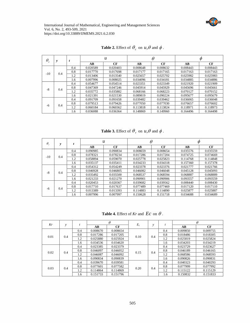
4.2 Comparision of AB and CF Fractional Derivatives for Various Values of the
Parameters in Tabular Form Here we compare between AB and CF fractional derivative for various values of the
parameters M , c , r , Sc , Kr , Pr , Ec taking 4.0y and 4.0t . From the following tables
it is found that the values of the velocity, temperature and concentration profiles for various
parameters are almost the same for both the methods- AB and CF fractional derivative.
Table 1. Effect of M on ,u and .
M y t u
AB CF AB CF AB CF
0.25 0.4
0.4 0.036610 0.036588 0.008659 0.008654 0.008459 0.008439
0.8 0.060779 0.060758 0.017286 0.017204 0.017143 0.017140
1.2 0.079966 0.079979 0.025779 0.025793 0.025928 0.025937
1.6 0.092290 0.092380 0.034333 0.034418 0.034799 0.034889
0.50 0.4
0.4 0.021852 0.021691 0.023380 0.023378 0.021848 0.021838
0.8 0.036248 0.036159 0.046098 0.046054 0.045382 0.045347
1.2 0.047737 0.047815 0.068543 0.068600 0.069422 0.069547
1.6 0.054954 0.054961 0.090805 0.090810 0.094434 0.094528
0.75 0.4
0.4 0.008157 0.008086 0.039695 0.039675 0.035782 0.035764
0.8 0.013610 0.013544 0.077713 0.077694 0.075483 0.075427
1.2 0.017888 0.017895 0.114888 0.114894 0.116372 0.116454
1.6 0.020577 0.020582 0.150742 0.151763 0.159960 0.159988
International Journal of Mathematical, Engineering and Management Sciences
Vol. 6, No. 2, 493-509, 2021
https://doi.org/10.33889/IJMEMS.2021.6.2.030
505
Table 2. Effect of c on ,u and .
c y t u
AB CF AB CF AB CF
-10 0.4
0.4 0.020589 0.020403 0.008648 0.008632 0.008443 0.008443
0.8 0.017770 0.017698 0.017177 0.017165 0.017163 0.017163
1.2 0.013406 0.013540 0.025657 0.025702 0.025982 0.025983
1.6 0.007996 0.008025 0.034096 0.034181 0.034885 0.034886
-8 0.4
0.4 0.054677 0.054514 0.023351 0.023349 0.021920 0.021909
0.8 0.047369 0.047246 0.045914 0.045929 0.045696 0.045661
1.2 0.035772 0.035882 0.068166 0.068223 0.070127 0.070152
1.6 0.021391 0.021530 0.089819 0.090224 0.095677 0.095679
-6 0.4
0.4 0.091709 0.091658 0.039482 0.039462 0.036065 0.036048
0.8 0.079513 0.079426 0.077050 0.077030 0.076657 0.076602
1.2 0.060184 0.060362 0.113818 0.113824 0.118971 0.118973
1.6 0.036088 0.036364 0.148869 0.149960 0.164496 0.164498
Table 3. Effect of r on ,u and .
r y t u
AB CF AB CF AB CF
-10 0.4
0.4 0.090985 0.090834 0.008659 0.008654 0.035576 0.035559
0.8 0.078321 0.078234 0.017286 0.017204 0.074725 0.074669
1.2 0.058894 0.059070 0.025778 0.025823 0.114768 0.114848
1.6 0.035137 0.035411 0.034233 0.034318 0.157360 0.157378
-8 0.4
0.4 0.054312 0.054249 0.023378 0.023376 0.021777 0.021766
0.8 0.046928 0.046805 0.046082 0.046048 0.045128 0.045093
1.2 0.035492 0.035500 0.068537 0.068594 0.068887 0.068889
1.6 0.021233 0.021270 0.090901 0.090906 0.093557 0.093559
-6 0.4
0.4 0.020453 0.020367 0.039682 0.039562 0.008440 0.008430
0.8 0.017710 0.017637 0.077489 0.077469 0.017120 0.017110
1.2 0.013389 0.013393 0.114883 0.114890 0.025877 0.025887
1.6 0.007996 0.007997 0.150628 0.151718 0.034688 0.034689
Table 4. Effect of Kr and Ec on .
Kr y t
Ec
y t
AB CF AB CF
0.01 0.4
0.4 0.008670 0.008654
0.10 0.4
0.4 0.009850 0.009755
0.8 0.017286 0.017205 0.8 0.018486 0.018305
1.2 0.025880 0.025924 1.2 0.025819 0.025824
1.6 0.034536 0.034620 1.6 0.034203 0.034219
0.02 0.4
0.4 0.023385 0.023379
0.15 0.4
0.4 0.023729 0.023627
0.8 0.046097 0.046052 0.8 0.046189 0.046165
1.2 0.046087 0.046092 1.2 0.068586 0.068593
1.6 0.090834 0.090839 1.6 0.090826 0.090831
0.03 0.4
0.4 0.039670 0.039581
0.20 0.4
0.4 0.040323 0.040293
0.8 0.077601 0.077582 0.8 0.077999 0.077992
1.2 0.114864 0.114869 1.2 0.115122 0.115129
1.6 0.151733 0.151796 1.6 0.150832 0.151833
International Journal of Mathematical, Engineering and Management Sciences
Vol. 6, No. 2, 493-509, 2021
https://doi.org/10.33889/IJMEMS.2021.6.2.030
506
Table 5. Effect of Pr on ,u and Sc on .
Pr y t u
Sc
AB CF AB CF AB CF
0.01 0.4
0.4 0.091703 0.091657 0.039570 0.039551
0.1
0.036467 0.036446
0.8 0.079509 0.079420 0.077501 0.077482 0.075666 0.075610
1.2 0.060472 0.060550 0.114864 0.114869 0.115655 0.115737
1.6 0.036469 0.036545 0.150733 0.151796 0.157770 0.157788
0.02 0.4
0.4 0.054574 0.054514 0.023375 0.023373
0.3
0.022380 0.022374
0.8 0.047387 0.047244 0.046087 0.046052 0.045518 0.045497
1.2 0.047294 0.047299 0.046087 0.046092 0.068746 0.068801
1.6 0.021586 0.021595 0.090734 0.090740 0.092652 0.092654
0.03 0.4
0.4 0.020487 0.020403 0.008659 0.008654
0.5
0.008556 0.008556
0.8 0.017770 0.017698 0.017386 0.017205 0.017153 0.017153
1.2 0.013476 0.013490 0.025880 0.025924 0.025755 0.025756
1.6 0.008922 0.008925 0.034316 0.034320 0.034360 0.034361
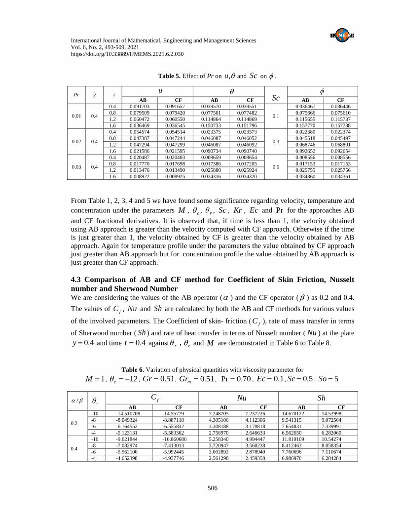
From Table 1, 2, 3, 4 and 5 we have found some significance regarding velocity, temperature and
concentration under the parameters M , c , r , Sc , Kr , Ec and Pr for the approaches AB
and CF fractional derivatives. It is observed that, if time is less than 1, the velocity obtained
using AB approach is greater than the velocity computed with CF approach. Otherwise if the time
is just greater than 1, the velocity obtained by CF is greater than the velocity obtained by AB
approach. Again for temperature profile under the parameters the value obtained by CF approach
just greater than AB approach but for concentration profile the value obtained by AB approach is
just greater than CF approach.
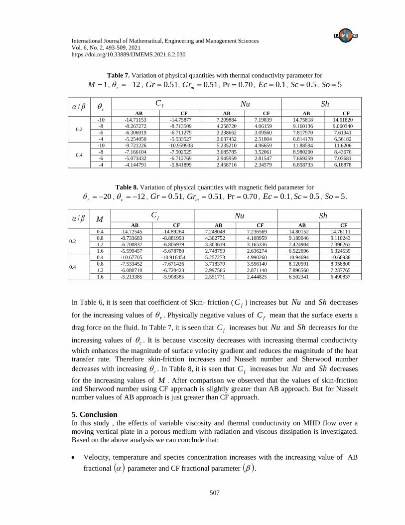
4.3 Comparison of AB and CF method for Coefficient of Skin Friction, Nusselt
number and Sherwood Number We are considering the values of the AB operator ( ) and the CF operator ( ) as 0.2 and 0.4.
The values of ,fC Nu and Sh are calculated by both the AB and CF methods for various values
of the involved parameters. The Coefficient of skin- friction ( fC ), rate of mass transfer in terms
of Sherwood number ( Sh ) and rate of heat transfer in terms of Nusselt number ( Nu ) at the plate
4.0y and time 4.0t against r , c and M are demonstrated in Table 6 to Table 8.
Table 6. Variation of physical quantities with viscosity parameter for
1M , 12c , 51.0Gr , 51.0mGr , 70.0Pr , 1.0Ec , 5.0Sc , 5So .
/ r fC Nu Sh
AB CF AB CF AB CF
0.2
-10 -14.510708 -14.55779 7.248705 7.237226 14.670122 14.52998
-8 -8.049324 -8.887118 4.305106 4.112306 9.541315 9.072564
-6 -6.164552 -6.555832 3.308188 3.170818 7.654831 7.339991
-4 -5.123131 -5.583362 2.756970 2.646633 6.562650 6.282060
0.4
-10 -9.621844 -10.860686 5.258340 4.994447 11.819109 10.54274
-8 -7.082974 -7.413013 3.720947 3.560238 8.412463 8.058354
-6 -5.562100 -5.992445 3.002892 2.878940 7.760696 7.110674
-4 -4.652398 -4.937746 2.561298 2.459358 6.986970 6.284284
International Journal of Mathematical, Engineering and Management Sciences
Vol. 6, No. 2, 493-509, 2021
https://doi.org/10.33889/IJMEMS.2021.6.2.030
507
Table 7. Variation of physical quantities with thermal conductivity parameter for
1M , 12r , 51.0Gr , 51.0mGr , 70.0Pr , 1.0Ec , 5.0Sc , 5So
/ c fC Nu Sh
AB CF AB CF AB CF
0.2
-10 -14.71153 -14.75877 7.209884 7.19839 14.75818 14.61820
-8 -8.267272 -8.713509 4.258720 4.06159 9.160136 9.060340
-6 -6.306919 -6.711279 3.238662 3.09560 7.817970 7.61941
-4 -5.254050 -5.533527 2.637452 2.51804 6.814178 6.56182
0.4
-10 -9.721226 -10.959933 5.235210 4.96659 11.88594 11.6206
-8 -7.166104 -7.502525 3.685785 3.52061 8.980200 8.43676
-6 -5.073432 -6.712769 2.945959 2.81547 7.669259 7.03681
-4 -4.144791 -5.841899 2.458716 2.34579 6.858733 6.18878
Table 8. Variation of physical quantities with magnetic field parameter for
20r , 12c , 51.0Gr , 51.0mGr , 70.0Pr , 1.0Ec , 5.0Sc , 5So .
/ M fC Nu Sh
AB CF AB CF AB CF
0.2
0.4 -14.72545 -14.89264 7.248048 7.236569 14.80152 14.76111
0.8 -8.733683 -8.881993 4.302752 4.108959 9.189046 9.110243
1.2 -6.700837 -6.806939 3.303619 3.165336 7.424904 7.396263
1.6 -5.599457 -5.678780 2.748759 2.636274 6.522696 6.324539
0.4
0.4 -10.67705 -10.916454 5.257273 4.990260 10.94694 10.66938
0.8 -7.533452 -7.671426 3.718370 3.556140 8.120591 8.058800
1.2 -6.080710 -6.720423 2.997566 2.871148 7.896560 7.237765
1.6 -5.213385 -5.908385 2.551771 2.444825 6.502341 6.490837
In Table 6, it is seen that coefficient of Skin- friction ( fC ) increases but Nu and Sh decreases
for the increasing values of r . Physically negative values of fC mean that the surface exerts a
drag force on the fluid. In Table 7, it is seen that fC increases but Nu and Sh decreases for the
increasing values of c . It is because viscosity decreases with increasing thermal conductivity
which enhances the magnitude of surface velocity gradient and reduces the magnitude of the heat
transfer rate. Therefore skin-friction increases and Nusselt number and Sherwood number
decreases with increasing c . In Table 8, it is seen that fC increases but Nu and Sh decreases
for the increasing values of M . After comparison we observed that the values of skin-friction
and Sherwood number using CF approach is slightly greater than AB approach. But for Nusselt
number values of AB approach is just greater than CF approach.
5. Conclusion In this study , the effects of variable viscosity and thermal conductuvity on MHD flow over a
moving vertical plate in a porous medium with radiation and viscous dissipation is investigated.
Based on the above analysis we can conclude that:
Velocity, temperature and species concentration increases with the increasing value of AB
fractional parameter and CF fractional parameter .
International Journal of Mathematical, Engineering and Management Sciences
Vol. 6, No. 2, 493-509, 2021
https://doi.org/10.33889/IJMEMS.2021.6.2.030
508
Magnetic field and viscosity have retarding effect in the flow.
Increasing value of Magnetic field parameter decreases the value of velocity but increases the
values of temperature and species concentration.
When the viscosity parameter increases, the velocity and the species concentration decreases
whereas temperature increases.
With the increasing thermal conductivity parameter, the velocity and the species
concentration increases but the temperature decreases.
Velocity and temperature increases with the increasing value of eckert number and radiation
parameter.
Velocity and temperature increases with the increasing value of prandlt number. Temperature
and species concentration decrease with the increasing value of the Schmidt number.
The values of the velocity, temperature and concentration profiles for various parameters are
almost the same for both the methods- AB and CF fractional derivatives. As gamma function
is present inside the exponential function in AB fractional derivative method, so the result
obtained by it is more accurate over the CF fractional derivative method.
Conflict of Interest The authors confirm that there is no conflict of interest to declare for this publication.
Acknowledgement The authors express their sincere thanks to the referees and the editor for their valuable comments and suggestions
towards the improvement of the paper.
References
Atangana, A., & Baleanu, D. (2016). New fractional derivatives with nonlocal and non-singular kernel:
Theory and application to heat transfer model. Thermal Science, 20(2), 763-769.
Aldoss, T.K., Al-Nimr, M.A., Jarrah, M.A., & Al-Sha'er, B.J. (1995). Magnetohydrodynamic mixed
convection from a vertical plate embedded in a porous medium. Numerical Heat Transfer, Part A:
Applications, 28(5), 635-645.
Khan, A., Ali Abro, K., Tassaddiq, A., & Khan, I. (2017). Atangana–Baleanu and Caputo Fabrizio analysis
of fractional derivatives for heat and mass transfer of second grade fluids over a vertical plate: a
comparative study. Entropy, 19(8), 279-290.
Bejan, A., & Khair, K.R. (1985). Heat and mass transfer by natural convection in a porous
medium. International Journal of Heat and Mass Transfer, 28(5), 909-918.
Hossain, M.A., & Munir, M.S. (2000). Mixed convection flow from a vertical flat plate with temperature
dependent viscosity. International Journal of Thermal Sciences, 39(2), 173-183.
Hristov, J. (2017). Steady-state heat conduction in a medium with spatial non-singular fading memory:
Derivation of Caputo-Fabrizio space-fractional derivative from Cattaneo concept with Jeffreys Kernel
and analytical solutions. Thermal science, 21(2), 827-839.
International Journal of Mathematical, Engineering and Management Sciences
Vol. 6, No. 2, 493-509, 2021
https://doi.org/10.33889/IJMEMS.2021.6.2.030
509
Javaherdeh, K., Nejad, M.M., & Moslemi, M. (2015). Natural convection heat and mass transfer in MHD
fluid flow past a moving vertical plate with variable surface temperature and concentration in a porous
medium. Engineering Science and Technology, an International Journal, 18(3), 423-431.
https://doi.org/10.1016/j.jestch.2015.03.001.
Lai, F.C., & Kulacki, F.A. (1990). The effects of variable viscosity on convective heat and mass transfer
along a vertical surface in standard porous media. International. Journal of Heat and Mass Transfer,
33(5), 1028-1031.
Mirza, I.A., & Vieru, D. (2017). Fundamental solutions to advection–diffusion equation with time-
fractional Caputo–Fabrizio derivative. Computers & Mathematics with Applications, 73(1), 1-10.
https://doi.org/10.1016/j.camwa.2016.09.026.
Mukhopadhyay, S., & Layek, G.C. (2008). Effects of thermal radiation and variable fluid viscosity on free
convective flow and heat transfer past a porous stretching surface. International Journal of Heat and
Mass Transfer, 51(6), 2167-2178.
Shah, N.A., & Khan, I. (2016). Heat transfer analysis in a second grade fluid over and oscillating vertical
plate using fractional Caputo–Fabrizio derivatives. The European Physical Journal C, 76(7), 362.
https://doi.org/10.1140/epjc/s10052-016-4209-3.
Sheikh, N.A., Ali, F., Saqib, M., Khan, I., Jan, S.A.A., Alshomrani, A.S., & Alghamdi, M.S. (2017).
Comparison and analysis of the Atangana–Baleanu and Caputo–Fabrizio fractional derivatives for
generalized Casson fluid model with heat generation and chemical reaction. Results in Physics, 7, 789-
800.
Original content of this work is copyright © International Journal of Mathematical, Engineering and Management Sciences. Uses
under the Creative Commons Attribution 4.0 International (CC BY 4.0) license at https://creativecommons.org/licenses/by/4.0/