Embed Size (px)
Citation preview
Hindawi Publishing CorporationDiscrete Dynamics in Nature and SocietyVolume 2011, Article ID 562494, 15 pagesdoi:10.1155/2011/562494
Research ArticleOn Riemann-Liouville and Caputo Derivatives
Changpin Li,1 Deliang Qian,2 and YangQuan Chen3
1 Department of Mathematics, Shanghai University, Shanghai 200444, China2 Department of Mathematics, Zhongyuan University of Technology, Zhengzhou 450007, China3 Department of Electrical and Computer Engineering, Utah State University, Logan, UT 84322-4120, USA
Correspondence should be addressed to Changpin Li, [email protected]
Received 27 June 2010; Accepted 25 January 2011
Academic Editor: Daniel Czamanski
Copyright q 2011 Changpin Li et al. This is an open access article distributed under the CreativeCommons Attribution License, which permits unrestricted use, distribution, and reproduction inany medium, provided the original work is properly cited.
Recently, many models are formulated in terms of fractional derivatives, such as in controlprocessing, viscoelasticity, signal processing, and anomalous diffusion. In the present paper, wefurther study the important properties of the Riemann-Liouville (RL) derivative, one of mostlyused fractional derivatives. Some important properties of the Caputo derivative which have notbeen discussed elsewhere are simultaneously mentioned. The partial fractional derivatives are alsointroduced. These discussions are beneficial in understanding fractional calculus and modelingfractional equations in science and engineering.
1. Introduction
Fractional calculus is not a new topic; in reality it has almost the same history as that of theclassical calculus [1]. Since the occurrence of fractional (or fractional-order) derivative, thetheories of fractional calculus (fractional derivative plus fractional integral) has undergonea significant and even heated development, which has been primarily contributed by purebut not applied mathematicians; the reader can refer to an encyclopedic book [2] andmany references cited therein. In the last few decades, however, applied scientists andengineers realized that differential equations with fractional derivative provided a naturalframework for the discussion of various kinds of real problems modeled by the aid offractional derivative, such as viscoelastic systems, signal processing, diffusion processes,control processing, fractional stochastic systems, allometry in biology and ecology ([3–17]and huge cited references therein).
Different from classical (or integer-order) derivative, there are several kinds ofdefinitions for fractional derivatives. These definitions are generally not equivalent with eachother. In the following, we introduce several definitions [7, 14].
2 Discrete Dynamics in Nature and Society
Definition 1.1. Yα, the convolution kernel of order α ∈ R+ for fractional integrals, is definedby
Yα(t) =tα−1+
Γ(α)∈ L1
loc(R+), (1.1)
where Γ is the well-known Euler Gamma function and
tα−1+ =
⎧⎨
⎩
tα−1, t > 0,
0, t ≤ 0.(1.2)
Definition 1.2. The fractional integral (or the Riemann-Liouville integral) D−α0,t with fractional
order α ∈ R+ of function x(t) is defined as
D−α0,t x(t) = Yα ∗ x(t) = 1
Γ(α)
∫ t
0(t − τ)α−1x(τ)dτ. (1.3)
Yα has an important convolution property (or semigroup property), that is, Yα ∗ Yβ =
Yα+β for arbitrary α > 0 and β > 0. This implies thatD−α0,t ·D
−β0,t = D
−α−β0,t .
Definition 1.3. The Grunwald-Letnikov fractional derivative with fractional order α isdefined by, if x(t) ∈ Cm[0, t],
GLDα0,tx(t) =
m−1∑
k=0
x(k)(0)t−α+k
Γ(−α + k + 1)
+1
Γ(m − α)
∫ t
0(t − τ)m−α−1x(m)(τ)dτ,
(1.4)
where m − 1 ≤ α < m ∈ Z+.
This is not the original definition. The initial definition is given by a limit, that is,
GLDα0,tx(t) = lim
h→ 0, nh=th−α
n∑
k=0
(−1)k(p
k
)
x(t − kh). (1.5)
The limit expression is not convenient for analysis but often used for numerical approxima-tion.
Discrete Dynamics in Nature and Society 3
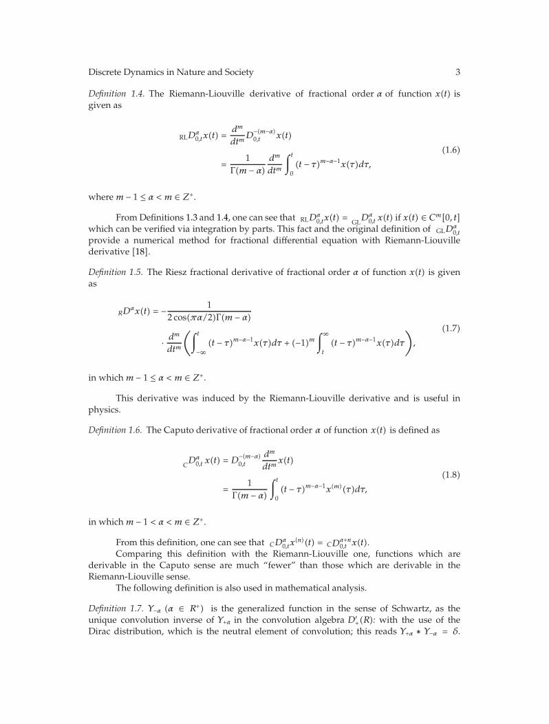
Definition 1.4. The Riemann-Liouville derivative of fractional order α of function x(t) isgiven as
RLDα0,tx(t) =
dm
dtmD
−(m−α)0,t x(t)
=1
Γ(m − α)dm
dtm
∫ t
0(t − τ)m−α−1x(τ)dτ,
(1.6)
where m − 1 ≤ α < m ∈ Z+.
FromDefinitions 1.3 and 1.4, one can see that RLDα0,tx(t) = GL
Dα0,t x(t) if x(t) ∈ Cm[0, t]
which can be verified via integration by parts. This fact and the original definition of GLDα0,t
provide a numerical method for fractional differential equation with Riemann-Liouvillederivative [18].
Definition 1.5. The Riesz fractional derivative of fractional order α of function x(t) is givenas
RDαx(t) = − 1
2 cos(πα/2)Γ(m − α)
· dm
dtm
(∫ t
−∞(t − τ)m−α−1x(τ)dτ + (−1)m
∫∞
t
(t − τ)m−α−1x(τ)dτ
)
,
(1.7)
in whichm − 1 ≤ α < m ∈ Z+.
This derivative was induced by the Riemann-Liouville derivative and is useful inphysics.
Definition 1.6. The Caputo derivative of fractional order α of function x(t) is defined as
CDα
0,t x(t) = D−(m−α)0,t
dm
dtmx(t)
=1
Γ(m − α)
∫ t
0(t − τ)m−α−1x(m)(τ)dτ,
(1.8)
in whichm − 1 < α < m ∈ Z+.
From this definition, one can see that CDα0,tx
(n)(t) = CDα+n0,t x(t).
Comparing this definition with the Riemann-Liouville one, functions which arederivable in the Caputo sense are much “fewer” than those which are derivable in theRiemann-Liouville sense.
The following definition is also used in mathematical analysis.
Definition 1.7. Y−α (α ∈ R+) is the generalized function in the sense of Schwartz, as theunique convolution inverse of Y+α in the convolution algebra D′
+(R): with the use of theDirac distribution, which is the neutral element of convolution; this reads Y+α ∗ Y−α = δ.
4 Discrete Dynamics in Nature and Society
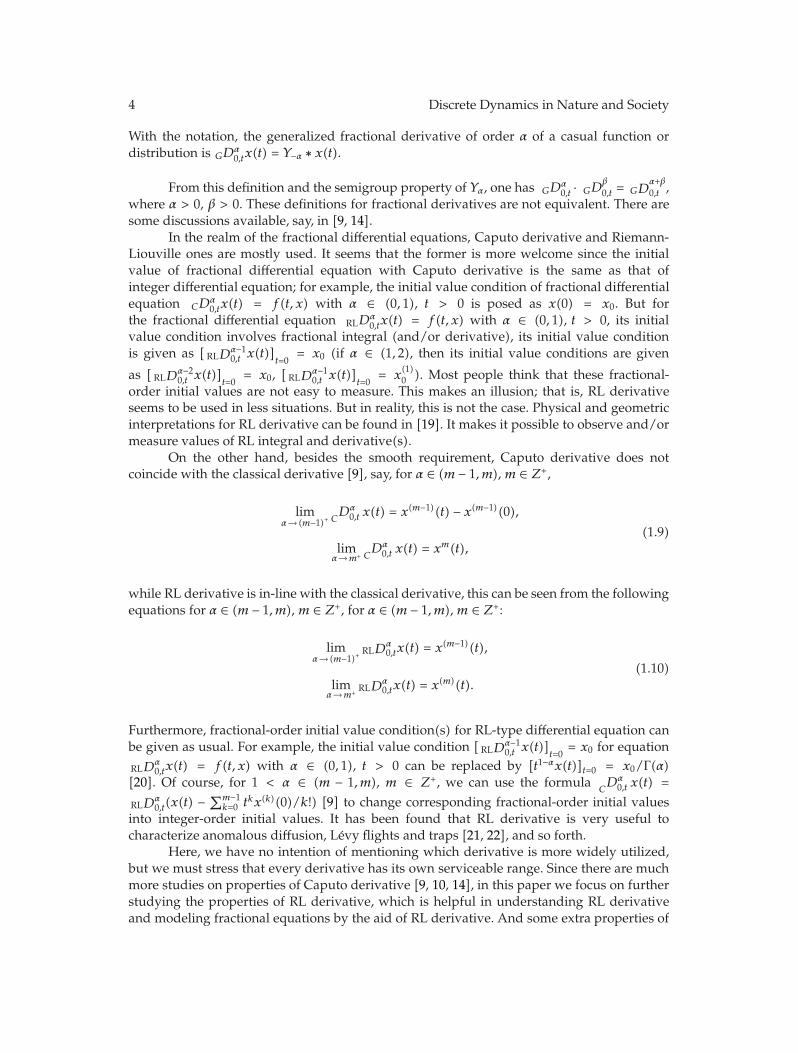
With the notation, the generalized fractional derivative of order α of a casual function ordistribution is GD
α0,tx(t) = Y−α ∗ x(t).
From this definition and the semigroup property of Yα, one has GDα0,t · GD
β0,t = GD
α+β0,t ,
where α > 0, β > 0. These definitions for fractional derivatives are not equivalent. There aresome discussions available, say, in [9, 14].
In the realm of the fractional differential equations, Caputo derivative and Riemann-Liouville ones are mostly used. It seems that the former is more welcome since the initialvalue of fractional differential equation with Caputo derivative is the same as that ofinteger differential equation; for example, the initial value condition of fractional differentialequation CD
α0,tx(t) = f(t, x) with α ∈ (0, 1), t > 0 is posed as x(0) = x0. But for
the fractional differential equation RLDα0,tx(t) = f(t, x) with α ∈ (0, 1), t > 0, its initial
value condition involves fractional integral (and/or derivative), its initial value conditionis given as [ RLD
α−10,t x(t)]t=0 = x0 (if α ∈ (1, 2), then its initial value conditions are given
as [ RLDα−20,t x(t)]t=0 = x0, [ RLD
α−10,t x(t)]t=0 = x
(1)0 ). Most people think that these fractional-
order initial values are not easy to measure. This makes an illusion; that is, RL derivativeseems to be used in less situations. But in reality, this is not the case. Physical and geometricinterpretations for RL derivative can be found in [19]. It makes it possible to observe and/ormeasure values of RL integral and derivative(s).
On the other hand, besides the smooth requirement, Caputo derivative does notcoincide with the classical derivative [9], say, for α ∈ (m − 1, m),m ∈ Z+,
limα→ (m−1)+ C
Dα0,t x(t) = x(m−1)(t) − x(m−1)(0),
limα→m+ C
Dα0,t x(t) = xm(t),
(1.9)
while RL derivative is in-line with the classical derivative, this can be seen from the followingequations for α ∈ (m − 1, m), m ∈ Z+, for α ∈ (m − 1, m),m ∈ Z+:
limα→ (m−1)+
RLDα0,tx(t) = x(m−1)(t),
limα→m+ RLD
α0,tx(t) = x(m)(t).
(1.10)
Furthermore, fractional-order initial value condition(s) for RL-type differential equation canbe given as usual. For example, the initial value condition [ RLD
α−10,t x(t)]t=0 = x0 for equation
RLDα0,tx(t) = f(t, x) with α ∈ (0, 1), t > 0 can be replaced by [t1−αx(t)]t=0 = x0/Γ(α)
[20]. Of course, for 1 < α ∈ (m − 1, m), m ∈ Z+, we can use the formulaCDα
0,t x(t) =
RLDα0,t(x(t) −
∑m−1k=0 tkx(k)(0)/k!) [9] to change corresponding fractional-order initial values
into integer-order initial values. It has been found that RL derivative is very useful tocharacterize anomalous diffusion, Levy flights and traps [21, 22], and so forth.
Here, we have no intention of mentioning which derivative is more widely utilized,but we must stress that every derivative has its own serviceable range. Since there are muchmore studies on properties of Caputo derivative [9, 10, 14], in this paper we focus on furtherstudying the properties of RL derivative, which is helpful in understanding RL derivativeand modeling fractional equations by the aid of RL derivative. And some extra properties of
Discrete Dynamics in Nature and Society 5
Caputo derivative are also introduced. The outline of the rest paper is organized as follows.In Section 2, we further study the important properties of RL derivative which have notappeared elsewhere. In the following section, we generalize the RL derivative to the RLpartial derivative. The last section includes conclusions.
2. Further Properties of RL and Caputo Derivatives
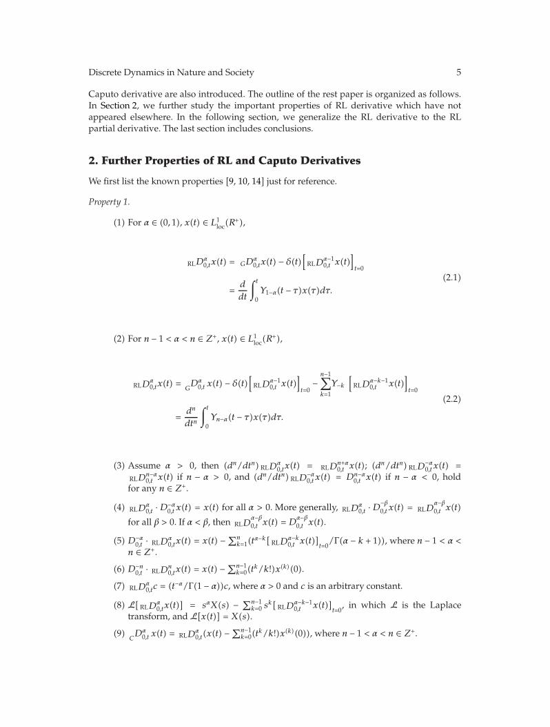
We first list the known properties [9, 10, 14] just for reference.
Property 1.
(1) For α ∈ (0, 1), x(t) ∈ L1loc(R
+),
RLDα0,tx(t) = GD
α0,tx(t) − δ(t)
[
RLDα−10,t x(t)
]
t=0
=d
dt
∫ t
0Y1−α(t − τ)x(τ)dτ.
(2.1)
(2) For n − 1 < α < n ∈ Z+, x(t) ∈ L1loc(R
+),
RLDα0,tx(t) = G
Dα0,t x(t) − δ(t)
[
RLDα−10,t x(t)
]
t=0−
n−1∑
k=1
Y−k[
RLDα−k−10,t x(t)
]
t=0
=dn
dtn
∫ t
0Yn−α(t − τ)x(τ)dτ.
(2.2)
(3) Assume α > 0, then (dn/dtn) RLDα0,tx(t) = RLD
n+α0,t x(t); (dn/dtn) RLD
−α0,tx(t) =
RLDn−α0,t x(t) if n − α > 0, and (dn/dtn) RLD
−α0,t x(t) = Dn−α
0,t x(t) if n − α < 0, holdfor any n ∈ Z+.
(4) RLDα0,t ·D−α
0,t x(t) = x(t) for all α > 0. More generally, RLDα0,t ·D
−β0,t x(t) = RLD
α−β0,t x(t)
for all β > 0. If α < β, then RLDα−β0,t x(t) = D
α−β0,t x(t).
(5) D−α0,t · RLD
α0,tx(t) = x(t) −∑n
k=1(tα−k[ RLD
α−k0,t x(t)]
t=0/Γ(α − k + 1)), where n − 1 < α <
n ∈ Z+.
(6) D−n0,t · RLD
n0,tx(t) = x(t) −∑n−1
k=0(tk/k!)x(k)(0).
(7) RLDα0,tc = (t−α/Γ(1 − α))c, where α > 0 and c is an arbitrary constant.
(8) L[ RLDα0,tx(t)] = sαX(s) − ∑n−1
k=0 sk[ RLD
α−k−10,t x(t)]
t=0, in which L is the Laplace
transform, and L[x(t)] = X(s).
(9)CDα
0,t x(t) = RLDα0,t(x(t) −
∑n−1k=0(t
k/k!)x(k)(0)), where n − 1 < α < n ∈ Z+.
6 Discrete Dynamics in Nature and Society
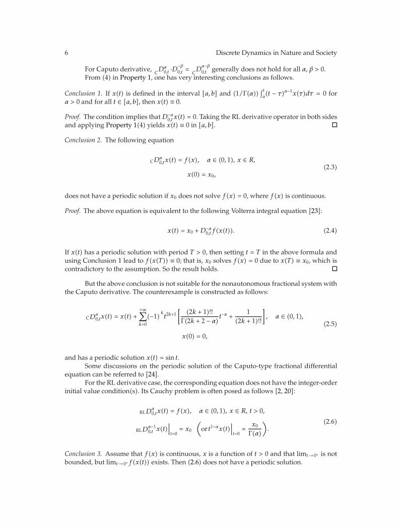
For Caputo derivative,CDα
0,t ·D−β0,t = C
Dα−β0,t generally does not hold for all α, β > 0.
From (4) in Property 1, one has very interesting conclusions as follows.
Conclusion 1. If x(t) is defined in the interval [a, b] and (1/Γ(α))∫ ta(t − τ)α−1x(τ)dτ = 0 for
α > 0 and for all t ∈ [a, b], then x(t) ≡ 0.
Proof. The condition implies thatD−α0,t x(t) = 0. Taking the RL derivative operator in both sides
and applying Property 1(4) yields x(t) ≡ 0 in [a, b].
Conclusion 2. The following equation
CDα0,tx(t) = f(x), α ∈ (0, 1), x ∈ R,
x(0) = x0,(2.3)
does not have a periodic solution if x0 does not solve f(x) = 0, where f(x) is continuous.
Proof. The above equation is equivalent to the following Volterra integral equation [23]:
x(t) = x0 +D−α0,t f(x(t)). (2.4)
If x(t) has a periodic solution with period T > 0, then setting t = T in the above formula andusing Conclusion 1 lead to f(x(T)) ≡ 0; that is, x0 solves f(x) = 0 due to x(T) ≡ x0, which iscontradictory to the assumption. So the result holds.
But the above conclusion is not suitable for the nonautonomous fractional system withthe Caputo derivative. The counterexample is constructed as follows:
CDα0,tx(t) = x(t) +
+∞∑
k=0
(−1) kt2k+1
[(2k + 1)!!
Γ(2k + 2 − α)t−α +
1(2k + 1)!!
]
, α ∈ (0, 1),
x(0) = 0,
(2.5)
and has a periodic solution x(t) = sin t.Some discussions on the periodic solution of the Caputo-type fractional differential
equation can be referred to [24].For the RL derivative case, the corresponding equation does not have the integer-order
initial value condition(s). Its Cauchy problem is often posed as follows [2, 20]:
RLDα0,tx(t) = f(x), α ∈ (0, 1), x ∈ R, t > 0,
RLDα−10,t x(t)
∣∣∣t=0
= x0
(
or t1−αx(t)∣∣∣t=0
=x0
Γ(α)
)
.(2.6)
Conclusion 3. Assume that f(x) is continuous, x is a function of t > 0 and that limt→ 0+ is notbounded, but limt→ 0+f(x(t)) exists. Then (2.6) does not have a periodic solution.

Discrete Dynamics in Nature and Society 7
Proof. Equation (2.6) is equivalent to the following integral equation [2, 20]:
x(t) =x0
Γ(α)tα−1 +D−α
0,t f(x(t)). (2.7)
If limt→ 0+ is bounded, then the case is trivial so it is omitted here. We only showinterests in the case that limt→ 0+ is not bounded. Suppose that (2.6) has a periodic solutionwith period T > 0, then, for arbitrary small δ > 0, one has x(δ) = x(δ+T). From (2.7), |x(δ+T)|has a bound independent of δ for arbitrary δ > 0 due to the assumption of f(x), but |x(t)|approaches to +∞ as δ → 0+. This completes Conclusion 3.
The previous conclusion can be very smoothly generalized to the higher-dimensionalcase. In the following, we further study the important nature of RL derivative.
Property 2.
(1) Composition with the integral operator: for α > 0, β > 0, then RLDα−β0,t = RLD
α0,t ·
D−β0,t /=D
−β0,t · RLD
α0,t.
(2) Composition with the integer derivative operator: for α ∈ (n−1, n), n ∈ Z+,m ∈ Z+,then (dm/dtm) · RLD
α0,t = RLD
α+m0,t /= RLD
α0,t · (dm/dtm).
(3) Composition with Caputo operator: for α ∈ (n − 1, n), n ∈ Z+, (α/= )β ∈ (m − 1, m),m ∈ Z+, then RLD
α+β−m0,t (dm/dtm) = RLD
α0,t · CD
β
0,t /= CD
β
0,t · RLDα0,t = D
−(m−β)0,t · RLDα+m
0,t .
(4) Composition with the generalized fractional derivative operator: for α ∈ (n − 1, n),n ∈ Z+, β > 0, then (dn/dtn)[Yn−α−β∗] = RLD
α0,t · G
Dβ
0,t /= GD
β
0,t · RLDα0,t = Y−β ∗ RLD
α0,t.
Proof. (1) Can be regarded as the direction conclusion of Property 1(4) and (5).(2) Can be derived by the direct computation.(3)Means that the RL derivative operators cannot commute with each other unless the
involved initial value conditions are homogeneous [14].(4) Can be proved by Property 1(2) and corresponding definitions.
Although the Riemann-Liouville integral operator D−α0,t (α ∈ R+) has the semigroup
property, that is, D−α0,t · D
−β0,t = D
−α−β0,t (α > 0, β > 0), RL derivative operator RLD
α0,t does not
have this character, that is, RLDα0,t · RLD
β
0,t /= RLDα+β0,t and RLD
β
0,t · RLDα0,t /= RLD
α+β0,t [14]. However,
we have following interesting result.
Property 3. If x(t) ∈ C1[0, T], αi ∈ (0, 1) (i = 1, 2) (the trivial case αi = 0 or 1 is simple andremoved here), and α1 + α2 ∈ (0, 1], then RLD
α10,t · RLD
α20,tx(t) = RLD
α1+α20,t x(t).
Proof. According to Property 1(3), one gets
CDα2
0,t · CDα10,t x(t) = C
Dα20,t
{
RLDα10,t[x(t) − x(0)]
}
= RLDα20,t
{
RLDα10,t[x(t) − x(0)] −
CDα1
0,t x(t)∣∣∣t=0
}
8 Discrete Dynamics in Nature and Society
= RLDα20,t
{
RLDα10,t[x(t) − x(0)]
}
= RLDα20,t · RLD
α10,tx(t) −
t−α1−α2
Γ(1 − α1 − α2)x(0).
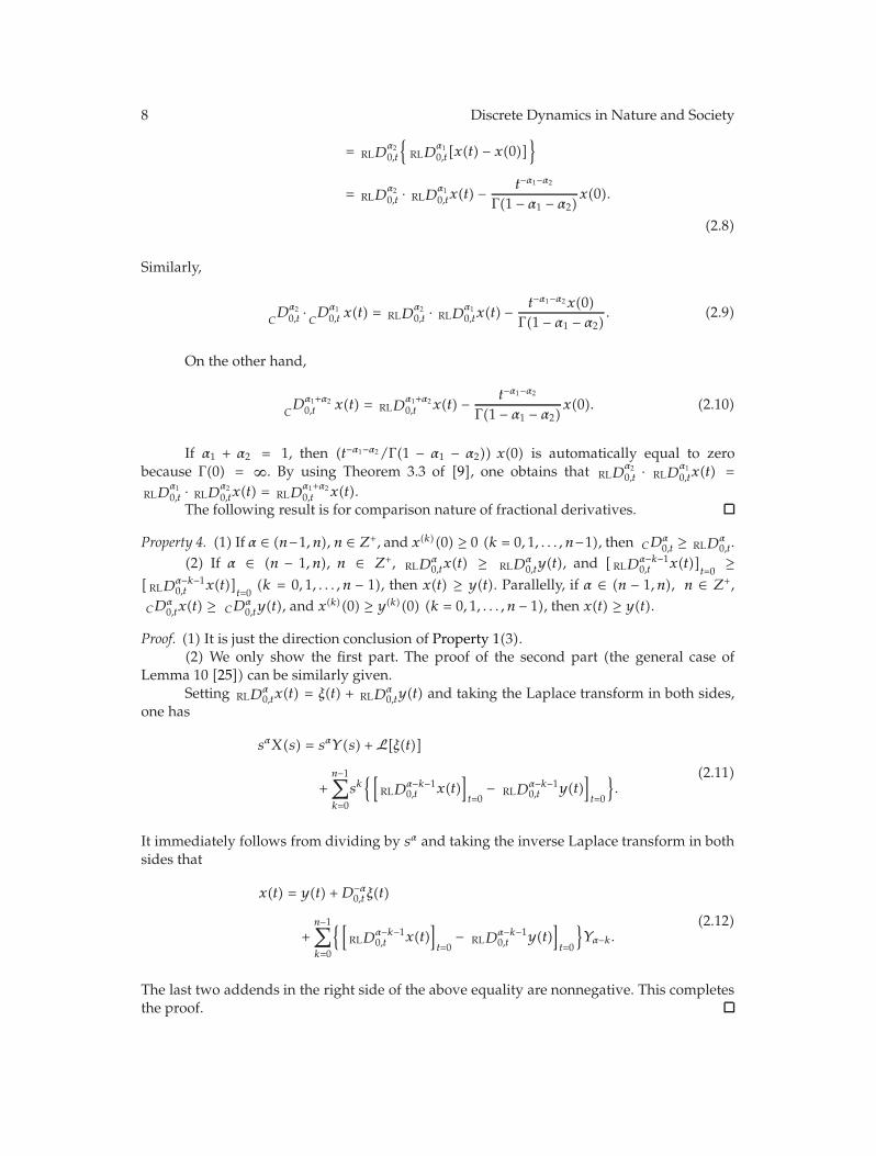
(2.8)
Similarly,
CDα2
0,t · CDα10,t x(t) = RLD
α20,t · RLD
α10,tx(t) −
t−α1−α2x(0)Γ(1 − α1 − α2)
. (2.9)
On the other hand,
CDα1+α2
0,t x(t) = RLDα1+α20,t x(t) − t−α1−α2
Γ(1 − α1 − α2)x(0). (2.10)
If α1 + α2 = 1, then (t−α1−α2/Γ(1 − α1 − α2)) x(0) is automatically equal to zerobecause Γ(0) = ∞. By using Theorem 3.3 of [9], one obtains that RLD
α20,t · RLD
α10,tx(t) =
RLDα10,t · RLD
α20,tx(t) = RLD
α1+α20,t x(t).
The following result is for comparison nature of fractional derivatives.
Property 4. (1) If α ∈ (n−1, n), n ∈ Z+, and x(k)(0) ≥ 0 (k = 0, 1, . . . , n−1), then CDα0,t ≥ RLD
α0,t.
(2) If α ∈ (n − 1, n), n ∈ Z+, RLDα0,tx(t) ≥ RLD
α0,ty(t), and [ RLD
α−k−10,t x(t)]
t=0≥
[ RLDα−k−10,t x(t)]
t=0(k = 0, 1, . . . , n − 1), then x(t) ≥ y(t). Parallelly, if α ∈ (n − 1, n), n ∈ Z+,
CDα0,tx(t) ≥ CD
α0,ty(t), and x(k)(0) ≥ y(k)(0) (k = 0, 1, . . . , n − 1), then x(t) ≥ y(t).
Proof. (1) It is just the direction conclusion of Property 1(3).(2) We only show the first part. The proof of the second part (the general case of
Lemma 10 [25]) can be similarly given.Setting RLD
α0,tx(t) = ξ(t) + RLD
α0,ty(t) and taking the Laplace transform in both sides,
one has
sαX(s) = sαY(s) +L[ξ(t)]
+n−1∑
k=0
sk{[
RLDα−k−10,t x(t)
]
t=0− RLD
α−k−10,t y(t)
]
t=0
}.
(2.11)
It immediately follows from dividing by sα and taking the inverse Laplace transform in bothsides that
x(t) = y(t) +D−α0,t ξ(t)
+n−1∑
k=0
{[
RLDα−k−10,t x(t)
]
t=0− RLD
α−k−10,t y(t)
]
t=0
}Yα−k.
(2.12)
The last two addends in the right side of the above equality are nonnegative. This completesthe proof.
Discrete Dynamics in Nature and Society 9
Property 5. Let A = {x(t) ∈ R, t ≥ 0, x(t) is analytical for any t ≥ 0}. If α ∈ (0, 1), then RLderivative operator RLD
α0,t defined in A can be expressed as
RLDα0,t =
∞∑
k=0
[dk · /dtk]t=0Γ(k − α + 1)
tk−α. (2.13)
More generally, if n − 1 < α < n ∈ Z+, then RLDα0,t defined inA has also the following form:
RLDα0,t =
∞∑
k=0
[dk · /dtk]t=0Γ(k − α + 1)
tk−α. (2.14)
The proof is easy so it is left out here.
Remark 2.1. (1) For an arbitrary function x(t) ∈ A, according to the expressions of Caputodifferential operator [10] and RL differential operator, one can also easy get Property 1(3).
(2) Even if x(t) ∈ A (it implies that x(0) exists), [ RLDα0,tx(t)]t=0(α > 0) may not exist
unless the initial value x(0) = 0.
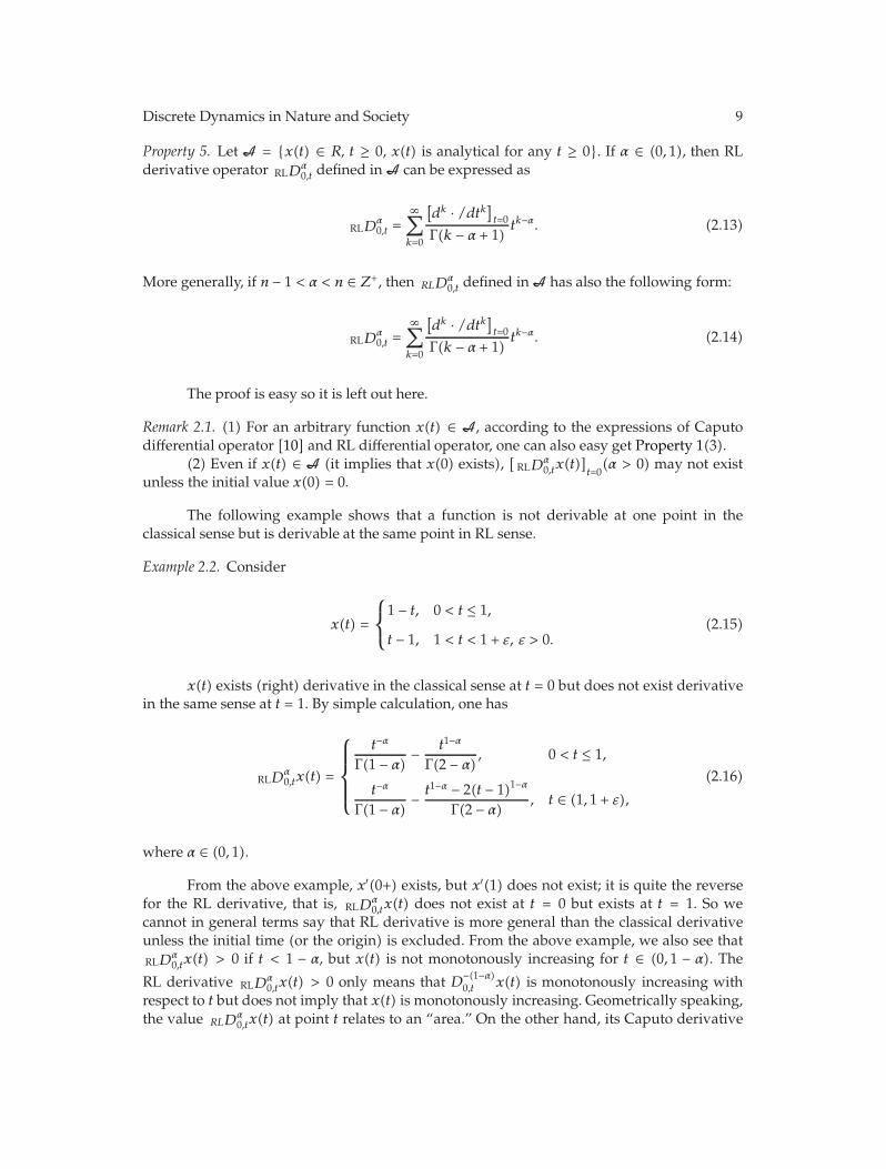
The following example shows that a function is not derivable at one point in theclassical sense but is derivable at the same point in RL sense.
Example 2.2. Consider
x(t) =
⎧⎨
⎩
1 − t, 0 < t ≤ 1,
t − 1, 1 < t < 1 + ε, ε > 0.(2.15)
x(t) exists (right) derivative in the classical sense at t = 0 but does not exist derivativein the same sense at t = 1. By simple calculation, one has
RLDα0,tx(t) =
⎧⎪⎪⎪⎨
⎪⎪⎪⎩
t−α
Γ(1 − α)− t1−α
Γ(2 − α), 0 < t ≤ 1,
t−α
Γ(1 − α)− t1−α − 2(t − 1)1−α
Γ(2 − α), t ∈ (1, 1 + ε),
(2.16)
where α ∈ (0, 1).
From the above example, x′(0+) exists, but x′(1) does not exist; it is quite the reversefor the RL derivative, that is, RLD
α0,tx(t) does not exist at t = 0 but exists at t = 1. So we
cannot in general terms say that RL derivative is more general than the classical derivativeunless the initial time (or the origin) is excluded. From the above example, we also see thatRLD
α0,tx(t) > 0 if t < 1 − α, but x(t) is not monotonously increasing for t ∈ (0, 1 − α). The
RL derivative RLDα0,tx(t) > 0 only means that D−(1−α)
0,t x(t) is monotonously increasing withrespect to t but does not imply that x(t) is monotonously increasing. Geometrically speaking,the value RLD
α0,tx(t) at point t relates to an “area.” On the other hand, its Caputo derivative
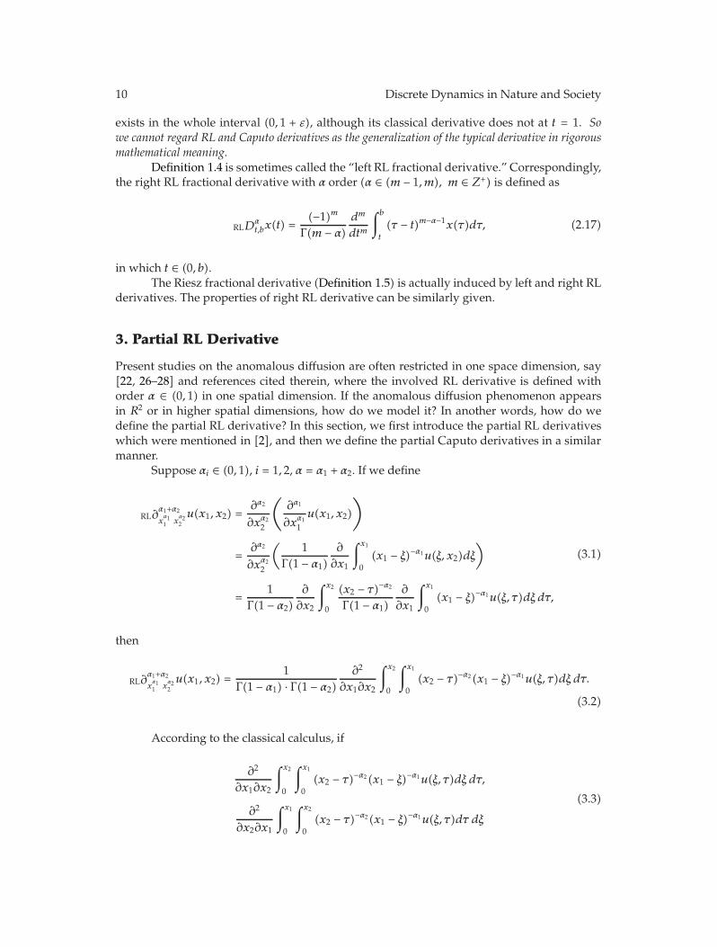
10 Discrete Dynamics in Nature and Society
exists in the whole interval (0, 1 + ε), although its classical derivative does not at t = 1. Sowe cannot regard RL and Caputo derivatives as the generalization of the typical derivative in rigorousmathematical meaning.
Definition 1.4 is sometimes called the “left RL fractional derivative.” Correspondingly,the right RL fractional derivative with α order (α ∈ (m − 1, m), m ∈ Z+) is defined as
RLDαt,bx(t) =
(−1)mΓ(m − α)
dm
dtm
∫b
t
(τ − t)m−α−1x(τ)dτ, (2.17)
in which t ∈ (0, b).The Riesz fractional derivative (Definition 1.5) is actually induced by left and right RL
derivatives. The properties of right RL derivative can be similarly given.
3. Partial RL Derivative
Present studies on the anomalous diffusion are often restricted in one space dimension, say[22, 26–28] and references cited therein, where the involved RL derivative is defined withorder α ∈ (0, 1) in one spatial dimension. If the anomalous diffusion phenomenon appearsin R2 or in higher spatial dimensions, how do we model it? In another words, how do wedefine the partial RL derivative? In this section, we first introduce the partial RL derivativeswhich were mentioned in [2], and then we define the partial Caputo derivatives in a similarmanner.
Suppose αi ∈ (0, 1), i = 1, 2, α = α1 + α2. If we define
RL∂α1+α2
xα11 x
α22u(x1, x2) =
∂α2
∂xα22
(∂α1
∂xα11
u(x1, x2)
)
=∂α2
∂xα22
(1
Γ(1 − α1)∂
∂x1
∫x1
0(x1 − ξ)−α1u(ξ, x2)dξ
)
=1
Γ(1 − α2)∂
∂x2
∫x2
0
(x2 − τ)−α2
Γ(1 − α1)∂
∂x1
∫x1
0(x1 − ξ)−α1u(ξ, τ)dξ dτ,
(3.1)
then
RL∂α1+α2
xα11 x
α22u(x1, x2) =
1Γ(1 − α1) · Γ(1 − α2)
∂2
∂x1∂x2
∫x2
0
∫x1
0(x2 − τ)−α2(x1 − ξ)−α1u(ξ, τ)dξ dτ.
(3.2)
According to the classical calculus, if
∂2
∂x1∂x2
∫x2
0
∫x1
0(x2 − τ)−α2(x1 − ξ)−α1u(ξ, τ)dξ dτ,
∂2
∂x2∂x1
∫x1
0
∫x2
0(x2 − τ)−α2(x1 − ξ)−α1u(ξ, τ)dτ dξ
(3.3)
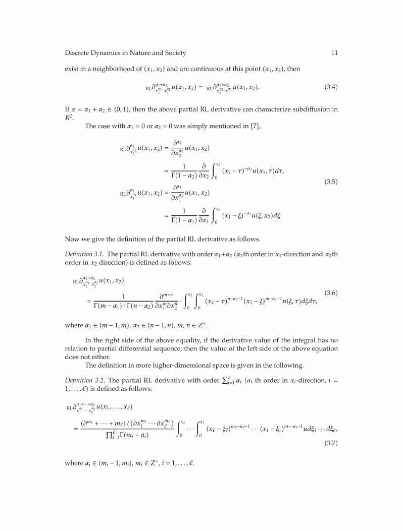
Discrete Dynamics in Nature and Society 11
exist in a neighborhood of (x1, x2) and are continuous at this point (x1, x2), then
RL∂α1+α2
xα11 x
α22u(x1, x2) = RL∂
α1+α2
xα22 x
α11u(x1, x2). (3.4)
If α = α1 + α2 ∈ (0, 1), then the above partial RL derivative can characterize subdiffusion inR2.
The case with α1 = 0 or α2 = 0 was simply mentioned in [7],
RL∂α2
xα22u(x1, x2) =
∂α2
∂xα22
u(x1, x2)
=1
Γ(1 − α2)∂
∂x2
∫x2
0(x2 − τ)−α2u(x1, τ)dτ,
RL∂α1
xα11u(x1, x2) =
∂α1
∂xα11
u(x1, x2)
=1
Γ(1 − α1)∂
∂x1
∫x1
0(x1 − ξ)−α1u(ξ, x2)dξ.
(3.5)
Now we give the definition of the partial RL derivative as follows.
Definition 3.1. The partial RL derivative with order α1+α2 (α1th order in x1-direction and α2thorder in x2 direction) is defined as follows:
RL∂α1+α2
xα11 x
α22u(x1, x2)
=1
Γ(m − α1) · Γ(n − α2)∂m+n
∂xm1 ∂x
n2·∫x2
0
∫x1
0(x2 − τ)n−α2−1(x1 − ξ)m−α1−1u(ξ, τ)dξdτ,
(3.6)
where α1 ∈ (m − 1, m), α2 ∈ (n − 1, n),m, n ∈ Z+.
In the right side of the above equality, if the derivative value of the integral has norelation to partial differential sequence, then the value of the left side of the above equationdoes not either.
The definition in more higher-dimensional space is given in the following.
Definition 3.2. The partial RL derivative with order∑
i=1 αi (αi th order in xi-direction, i =1, . . . , ) is defined as follows:
RL∂α1+···+α
xα11 ··· xα
u(x1, . . . , x)
=(∂m1 + · · · +m)/
(∂xm1
1 · · ·∂xm
)
∏i=1Γ(mi − αi)
∫x
0· · ·∫x1
0(x − ξ)m−α−1 · · · (x1 − ξ1)m1−α1−1udξ1 · · ·dξ,
(3.7)
where αi ∈ (mi − 1, mi), mi ∈ Z+, i = 1, . . . , .
12 Discrete Dynamics in Nature and Society
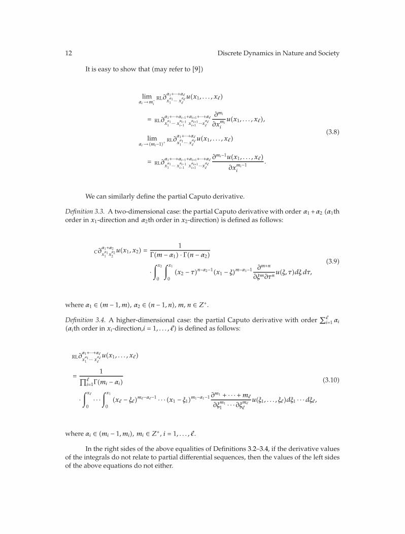
It is easy to show that (may refer to [9])
limαi →m−
i
RL∂α1+···+α
xα11 ··· xα
u(x1, . . . , x)
= RL∂α1+···+αi−1+αi+1+···+α
xα11 ··· xαi−1
i−1 xαi+1i+1 ···xα
∂mi
∂xmi
i
u(x1, . . . , x),
limαi → (mi−1)+
RL∂α1+···+α
xα11 ··· xα
u(x1, . . . , x)
= RL∂α1+···+αi−1+αi+1+···+α
xα11 ··· xαi−1
i−1 xαi+1i+1 ···xα
∂mi−1u(x1, . . . , x)
∂xmi−1i
.
(3.8)
We can similarly define the partial Caputo derivative.
Definition 3.3. A two-dimensional case: the partial Caputo derivative with order α1 +α2 (α1thorder in x1-direction and α2th order in x2-direction) is defined as follows:
C∂α1+α2
xα11 x
α22u(x1, x2) =
1Γ(m − α1) · Γ(n − α2)
·∫x2
0
∫x1
0(x2 − τ)n−α2−1(x1 − ξ)m−α1−1 ∂m+n
∂ξm∂τnu(ξ, τ)dξ dτ,
(3.9)
where α1 ∈ (m − 1, m), α2 ∈ (n − 1, n),m, n ∈ Z+.
Definition 3.4. A higher-dimensional case: the partial Caputo derivative with order∑
i=1 αi
(αith order in xi-direction,i = 1, . . . , ) is defined as follows:
RL∂α1+···+α
xα11 ··· xα
u(x1, . . . , x)
=1
∏i=1Γ(mi − αi)
·∫x
0· · ·∫x1
0(x − ξ)m−α−1 · · · (x1 − ξ1)
m1−α1−1 ∂m1 + · · · +m
∂ξm11 · · ·∂ξm
u(ξ1, . . . , ξ)dξ1 · · ·dξ,
(3.10)
where αi ∈ (mi − 1, mi), mi ∈ Z+, i = 1, . . . , .
In the right sides of the above equalities of Definitions 3.2–3.4, if the derivative valuesof the integrals do not relate to partial differential sequences, then the values of the left sidesof the above equations do not either.
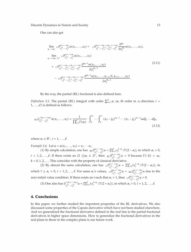
Discrete Dynamics in Nature and Society 13
One can also get
limαi →m−
i
C∂α1+···+α
xα11 ··· xα
u(x1, . . . , x) = C∂α1+···+αi−1+αi+1+···+α
xα11 ··· xαi−1
i−1 xαi+1i+1 ···xα
∂mi
∂xmi
i
u(x1, . . . , x),
limαi → (mi−1)+
C∂α1+···+α
xα11 ··· xα
u(x1, . . . , x)
= C∂α1+···+αi−1+αi+1+···+α
xα11 ··· xαi−1
i−1 xαi+1i+1 ···xα
∂mi−1u(x1, . . . , x)
∂xmi−1i
− C∂α1+···+αi−1+αi+1+···+α
xα11 ··· xαi−1
i−1 xαi+1i+1 ···xα
∂mi−1u(x1, . . . , xi−1, 0, xi+1, . . . , x)
∂xmi−1i
.
(3.11)
By the way, the partial (RL) fractional is also defined here.
Definition 3.5. The partial (RL) integral with order∑
i=1 αi (αi th order in xi-direction, i =1, . . . , ) is defined as follows:
RL∂−(α1+···+α)
xα11 ··· xα
u(x1, . . . , x) =1
∏i=1Γ(αi)
·∫x
0· · ·∫x1
0(x − ξ)α−1 · · · (x1 − ξ1)α1−1udξ1 · · ·dξ,
(3.12)
where αi ∈ R+, i = 1, . . . , .
Example 3.6. Let u = u(x1, . . . , x) = x1 · · ·x .(1) By simple calculation, one has RL∂
α1+···+α
xα11 ··· xα
u =∏
i=1x1−αi
i /Γ(2 − αi), in which αi > 0,
i = 1, 2, . . . , . If there exists an (2 ≤)αi ∈ Z+, then RL∂α1+···+α
xα11 ··· xα
u = 0 because Γ(−k) = ∞,
k = 0, 1, 2, . . .. This coincides with the property of classical derivative.(2) By almost the same calculation, one has C∂
α1+···+α
xα11 ··· xα
u =∏
i=1(x1−αi
i /Γ(2 − αi)), in
which 1 ≥ αi > 0, i = 1, 2, . . . , . For same αi’s values, C∂α1+···+α
xα11 ··· xα
u = RL∂α1+···+α
xα11 ··· xα
u due to the
zero initial value condition. If there exists an i such that αi > 1, then C∂α1+···+α
xα11 ··· xα
u = 0.
(3) One also has ∂−(α1+···+α)
xα11 ··· xα
u =∏
i=1(x1+αi
i /Γ(2 + αi)), in which αi > 0, i = 1, 2, . . . , .
4. Conclusions
In this paper, we further studied the important properties of the RL derivatives. We alsodiscussed some properties of the Caputo derivative which have not been studied elsewhere.And we generalized the fractional derivative defined in the real line to the partial fractionalderivatives in higher space dimensions. How to generalize the fractional derivatives in thereal plane to those in the complex plane is our future work.
14 Discrete Dynamics in Nature and Society
Acknowledgments
The presentworkwas supported in part by the National Natural Science Foundation of Chinaunder Grant no. 10872119 and the Key Disciplines of Shanghai Municipality under Grant no.S30104.
References
[1] K. S. Miller and B. Ross, An Introduction to the Fractional Calculus and Fractional Differential Equations,John Wiley & Sons, New York, NY, USA, 1993.
[2] S. G. Samko, A. A. Kilbas, and O. I. Marichev, Fractional Integrals and Derivatives, Gordon and BreachScience, Yverdon, Switzerland, 1993.
[3] D. Baleanu, K. Diethelm, E. Scalas, and J. J. Trujillo, Fractional Calculus Models and Numerical Methods,World Scientific, Singapore, 2009.
[4] P. L. Butzer and U. Westphal, An Introduction to Fractional Calculus, World Scientific, Singapore, 2000.[5] J. Guy, “Modeling fractional stochastic systems as non-random fractional dynamics driven by
Brownian motions,” Applied Mathematical Modelling, vol. 32, no. 5, pp. 836–859, 2008.[6] R. Hilfer, Applications of Fractional Calculus in Physics, World Scientific, River Edge, NJ, USA, 2000.[7] A. A. Kilbas, H. M. Srivastava, and J. J. Trujillo, Theory and Applications of Fractional Differential
Equations, vol. 204 of North-Holland Mathematics Studies, Elsevier, Amsterdam, The Netherlands,2006.
[8] I. Lakshmikantham and S. Leela, Theory of Fractional Dynamical Systems, Cambridge ScientificPublishers, Cambridge, UK, 2009.
[9] C. P. Li and W. H. Deng, “Remarks on fractional derivatives,” Applied Mathematics and Computation,vol. 187, no. 2, pp. 777–784, 2007.
[10] C. P. Li, X. H. Dao, and P. Guo, “Fractional derivatives in complex planes,” Nonlinear Analysis. Theory,Methods & Applications, vol. 71, no. 5-6, pp. 1857–1869, 2009.
[11] C. P. Li, Z. Q. Gong, D. L. Qian, and Y. Q. Chen, “On the bound of the Lyapunov exponents for thefractional differential systems,” Chaos, vol. 20, no. 1, Article ID 013127, 7 pages, 2010.
[12] K. B. Oldham and J. Spanier, The Fractional Calculus, Academic Press, New York, NY, USA, 1974.[13] M. D. Ortigueira, “Comments on “Modeling fractional stochastic systems as non-random fractional
dynamics driven Brownian motions”,” Applied Mathematical Modelling, vol. 33, no. 5, pp. 2534–2537,2009.
[14] I. Podlubny, Fractional Differential Equations, vol. 198 of Mathematics in Science and Engineering,Academic Press, New York, NY, USA, 1999.
[15] D. L. Qian, C. P. Li, R. P. Agarwal, and P. J. Y. Wong, “Stability analysis of fractional differentialsystem with Riemann-Liouville derivative,”Mathematical and Computer Modelling, vol. 52, no. 5-6, pp.862–874, 2010.
[16] B. J. West, M. Bologna, and P. Grigolini, Physics of Fractal Operators, Springer, New York, NY, USA,2003.
[17] Z. G. Zhao, Q. Guo, and C. P. Li, “A fractional model for the allometric scaling laws,” The Open AppliedMathematics Journal, vol. 2, pp. 26–30, 2008.
[18] S. B. Yuste and L. Acedo, “An explicit finite difference method and a new vonNeumann-type stabilityanalysis for fractional diffusion equations,” SIAM Journal on Numerical Analysis, vol. 42, no. 5, pp.1862–1874, 2005.
[19] N. Heymans and I. Podlubny, “Physical interpretation of initial conditions for fractional differentialequations with Riemann-Liouville fractional derivatives,” Rheologica Acta, vol. 45, no. 5, pp. C765–C771, 2006.
[20] S. Zhang, “Monotone iterative method for initial value problem involving Riemann-Liouvillefractional derivatives,” Nonlinear Analysis. Theory, Methods & Applications, vol. 71, no. 5-6, pp. 2087–2093, 2009.
[21] V. J. Ervin, N. Heuer, and J. P. Roop, “Numerical approximation of a time dependent, nonlinear, space-fractional diffusion equation,” SIAM Journal on Numerical Analysis, vol. 45, no. 2, pp. 572–591, 2007.
[22] P. Zhuang, F. Liu, V. Anh, and I. Turner, “New solution and analytical techniques of the implicitnumerical method for the anomalous subdiffusion equation,” SIAM Journal on Numerical Analysis,vol. 46, no. 2, pp. 1079–1095, 2008.
Discrete Dynamics in Nature and Society 15
[23] K. Diethelm and N. J. Ford, “Analysis of fractional differential equations,” Journal of MathematicalAnalysis and Applications, vol. 265, no. 2, pp. 229–248, 2002.
[24] M. S. Tavazoei and M. Haeri, “A proof for non existence of periodic solutions in time invariantfractional order systems,” Automatica, vol. 45, no. 8, pp. 1886–1890, 2009.
[25] Y. Li, Y. Q. Chen, and I. Podlubny, “Mittag-Leffer stability of fractional order nonlinear dynamicsystems,” Automatica, vol. 45, pp. 1965–1969, 2009.
[26] H. G. Sun, W. Chen, C. P. Li, and Y. Q. Chen, “Fractional differential models for anomalous diffusion,”Physica A, vol. 389, no. 14, pp. 2719–2724, 2010.
[27] Y. Y. Zheng, C. P. Li, and Z. G. Zhao, “A note on the finite element method for the space-fractionaladvection diffusion equation,” Computers & Mathematics with Applications, vol. 59, no. 5, pp. 1718–1726, 2010.
[28] Y. Y. Zheng, C. P. Li, and Z. G. Zhao, “A fully discrete discontinuous Galerkin method for nonlinearfractional fokker-planck equation,”Mathematical Problems in Engineerings, vol. 2010, Article ID 279038,26 pages, 2010.

Submit your manuscripts athttp://www.hindawi.com
Hindawi Publishing Corporationhttp://www.hindawi.com Volume 2014
MathematicsJournal of
Hindawi Publishing Corporationhttp://www.hindawi.com Volume 2014
Mathematical Problems in Engineering
Hindawi Publishing Corporationhttp://www.hindawi.com
Differential EquationsInternational Journal of
Volume 2014
Applied MathematicsJournal of
Hindawi Publishing Corporationhttp://www.hindawi.com Volume 2014
Probability and StatisticsHindawi Publishing Corporationhttp://www.hindawi.com Volume 2014
Journal of
Hindawi Publishing Corporationhttp://www.hindawi.com Volume 2014
Mathematical PhysicsAdvances in
Complex AnalysisJournal of
Hindawi Publishing Corporationhttp://www.hindawi.com Volume 2014
OptimizationJournal of
Hindawi Publishing Corporationhttp://www.hindawi.com Volume 2014
CombinatoricsHindawi Publishing Corporationhttp://www.hindawi.com Volume 2014
International Journal of
Hindawi Publishing Corporationhttp://www.hindawi.com Volume 2014
Operations ResearchAdvances in
Journal of
Hindawi Publishing Corporationhttp://www.hindawi.com Volume 2014
Function Spaces
Abstract and Applied AnalysisHindawi Publishing Corporationhttp://www.hindawi.com Volume 2014
International Journal of Mathematics and Mathematical Sciences
Hindawi Publishing Corporationhttp://www.hindawi.com Volume 2014
The Scientific World JournalHindawi Publishing Corporation http://www.hindawi.com Volume 2014
Hindawi Publishing Corporationhttp://www.hindawi.com Volume 2014
Algebra
Discrete Dynamics in Nature and Society
Hindawi Publishing Corporationhttp://www.hindawi.com Volume 2014
Hindawi Publishing Corporationhttp://www.hindawi.com Volume 2014
Decision SciencesAdvances in
Discrete MathematicsJournal of
Hindawi Publishing Corporationhttp://www.hindawi.com
Volume 2014 Hindawi Publishing Corporationhttp://www.hindawi.com Volume 2014
Stochastic AnalysisInternational Journal of