Astrophysical Applications of Gravitational Microlensing

Dissertation

Presented in Partial Fulfillment of the Requirements for the Degree Doctor ofPhilosophy in the Graduate School of The Ohio State University

By

Subo Dong, M.S.

Graduate Program in Astronomy

The Ohio State University

2009

Dissertation Committee:

Professor Andrew Philip Gould, Advisor

Professor Bernard Scott Gaudi

Professor Krzysztof Zbigniew Stanek

Copyright by

Subo Dong

2009

ABSTRACT

In this thesis, I present several astrophysical applications of Galactic and

cosmological microlensing.

The first few topics are on searching and characterizing extrasolar planets

by means of high-magnification microlensing events. The detection efficiency

analysis of the Amax ∼ 3000 event OGLE-2004-BLG-343 is presented. Due to

human error, intensive monitoring did not begin until 43 minutes after peak, at

which point the magnification had fallen to A ∼ 1200. It is shown that, had a

similar event been well sampled over the peak, it would have been sensitive to

almost all Neptune-mass planets over a factor of 5 in projected separation and even

would have had some sensitivity to Earth-mass planets. New algorithms optimized

for fast evaluation of binary-lens models with finite-sources effects have been

developed. These algorithms have enabled efficient and thorough parameter-space

searches in modeling planetary high-magnification events. The detection of the

cool, Jovian-mass planet MOA-2007-BLG-400Lb, discovered from an Amax = 628

event with severe finite-source effects, is reported. Detailed analysis yields a

fairly precise planet/star mass ratio of q = (2.5+0.5−0.3) × 10−3, while the planet/star

ii

projected separation is subject to a strong close/wide degeneracy. Photometric

and astrometric measurements from Hubble Space Telescope, as well as constraints

from higher order effects extracted from the ground-based light curve (microlens

parallax, planetary orbital motion and finite-source effects) are used to constrain the

nature of planetary event OGLE-2005-BLG-071Lb. Our primary analysis leads to

the conclusion that the host is an M = 0.46 ± 0.04 M⊙ M dwarf and that the planet

has mass Mp = 3.8 ± 0.4 MJupiter, which is likely to be the most massive planet yet

discovered that is hosted by an M dwarf.

Next a spaced-based microlens parallax is determined for the first time using

Spitzer and ground-based observations for binary-lens event OGLE-2005-SMC-001.

The parallax measurement yields a projected velocity v ∼ 230 km s−1, the typical

value expected for halo lenses, but an order of magnitude smaller than would be

expected for lenses lying in the Small Magellanic Cloud (SMC) itself.

Finally, I propose using quasar microlensing to probe Mg II and other

absorption “cloudlets” with sizes ∼ 10−4.0 − 10−2.0pc in the intergalactic medium.

I show that significant spectral variability on timescales of months to years can be

induced by such small-scale absorption “cloudlets” toward a microlensed quasar.

With numerical simulations, I demonstrate the feasibility of applying this method

to Q2237+0305, and I show that high-resolution spectra of this quasar in the near

future would provide a clear test of the existence of such metal-line absorbing

“cloudlets”.

iii

Dedicated to my mother and father

iv

ACKNOWLEDGMENTS

In modern times, most of the necessities of people’s daily lives rely upon others,

therefore, no matter how highly the lofty ideal of individual freedom is acclaimed,

most people have to choose their jobs according to the needs of the society rather

than following their inner voices (i.e., what they are interested in the most). I

consider myself very lucky to have five years’ opportunity to pursue my childhood

dream in becoming an astronomer with no financial burden. I am thankful to

everyone who has made this possible.

I thank Andy Gould for being an unparalleled advisor. He has taken immense

care in guiding me along my path to becoming a scientist. His influence and help

have permeated every aspect of my scientific activities as a graduate student.

Whenever I need discussions or advice (or whenever he perceives me as needing

them), he is always ready to offer them in most timely fashion. His excitement by

new findings, creativity in novel ideas, and self-driven “Gung-ho” working spirit

exhibit no trace of his age. It is difficult to describe how exhilarating an experience

it is to work with him.

v

I thank Andy for being a truthful person – for being truthful to himself, to

others, and to nature. I was initially intimidated by the way he spoke in morning

coffee and colloquia. But I have come to realize that, if one is offended by sincere

efforts to pursue the truth, or not offended by distortion or fabrication of facts and

careless or superficial analyses, he/she is not a real scientist. I thank Andy for

teaching me to be honest to data, to listen to what nature has to say rather than

projecting one’s prejudices onto nature.

I came to the United States certainly at an interesting time, when “the best and

brightest” in the White House and on the Wall Street have drastically transformed

the world’s social and economic orders. As a “Stranger in a Strange Land”, I

appreciate Andy for many illuminating discussions that shed light on the perplexing

and intriguing events in the U.S. and on the world stage. He observes the society at a

vantage point beyond his ethnical, national, and cultural background. I never have to

worry about offending him by expressing my honest views. I thank Andy for rallying

a group of people (mostly astronomers) to have discussions on real-world events in

a similar fashion as we discuss science. We attempt to distinguish between real and

bogus information from various sources and analyze the events by confronting ideas

against distilled evidence and data. Although I do not always agree with Andy, it

has always been such a great time talking to him on almost anything.

Next I thank my thesis committee members, Scott Gaudi and Kris Stanek.

vi

I first met Scott back when he was a postdoc at CfA. He has been providing

unreserved encouragement and support to me since then. I have benefited greatly

from his advice on science and professional development. I thank him for having

led me to see the bright side when I was in depression or frustration. I admire

his comprehensive knowledge in almost all branches of astronomy and his often

amazingly deep physical intuition.

I thank Kris for being friendly and humorous and willing to talk to me on any

topic. I thank him for inspiring discussions that led to my first original workable

science idea. I appreciate his insistence that scientific pictures should fundamentally

be simple. He always has great insights into complexity and sees through irrelevant

artificial obscuration. I hope I will be able to acquire even a fraction of his ability in

seizing the moments by recognizing fleeting opportunities in astronomy.

I am grateful to Rick Pogge, Chris Kochanek and many others in the department

for providing a lot of great technical help and having interesting science discussions

together. And I greatly appreciate many faculty in the department for creating an

intellectually stimulating environment which is also very student-friendly. Daily

coffee has become an indispensable part of my life. The department staff are

always helpful, and I especially thank David Will for solving many of my computer

problems.

vii

I have spent a great time with many graduate students and several postdocs at

OSU. I first thank Zheng for having provided me many great advice when I first got

to OSU, and for him being a role-model student and astronomer. He shows me how

high someone with a similar background as me can possibly achieve in astronomy. I

thank Jose, Vimal, Dale, Himel and others for having a lot of interesting discussions

and experience together. And I appreciate having many great office mates, Frank,

Molly, Ondrej, Kelly, Rob, Deokkeun, etc., during the last five years. Szymon and

Xinyu have been great friends and colleagues.

I could not possibly have finished my PhD work without many colleagues

outside Ohio State. In particular, I thank Andrzej Udalski for being an exemplary

astronomer. I never fail to be thrilled by the first-rate data he and the OGLE team

have produced. A lot of crucial data I have analyzed come from many “amateur”

astronomers: Jennie McCormick, Grant Christie and Berto Monard, to name a few.

They are amateurs only in the sense that they are not paid for their observations,

otherwise what they do are extraordinarily professional. Their fascination in the sky,

enthusiasm and dedication have been a constant source of inspiration to me. I thank

all my observer colleagues for offering me the privilege in being the first to see many

beautiful light curves and realize the exotic extrasolar worlds that they reveal. The

precious moments of discovery transcend anything else.

viii

I wish to express my deep gratitude to Profs. Dawei Yang, Tianyi Huang,

Qiusheng Gu and Dr. Jin Zhu for their selfless help and great guidance at various

important stages before I entered the graduate school.

At last, I thank my mother and father, who put my education, both in acquiring

knowledge and in being a decent member of the society, as the first priority in

their life. Without their unequivocal support and sacrifice, I would have never been

anywhere near the position I am at today to write this dissertation.

ix

VITA

March 18, 1982 . . . . . . . . . . . . . . . . Born – Chengde, Hebei, China

2004 . . . . . . . . . . . . . . . . . . . . . . . . . . . B.S. Astronomy, Nanjing University, China

2004 – 2005 . . . . . . . . . . . . . . . . . . . . University Fellow, The Ohio State University

2005 – 2006 . . . . . . . . . . . . . . . . . . . . Graduate Research Assistant,

The Ohio State University

2006 . . . . . . . . . . . . . . . . . . . . . . . . . . . M.S. Astronomy, The Ohio State University

2006 – 2008 . . . . . . . . . . . . . . . . . . . . Graduate Research and Teaching Assistant,

The Ohio State University

2008 – 2009 . . . . . . . . . . . . . . . . . . . . . Presidential Fellow, The Ohio State University

PUBLICATIONS

Research Publications

1. A. Udalski, et al. “A Jovian-Mass Planet in Microlensing Event OGLE-2005-BLG-071”, ApJL, 628, 109L, (2005).

2. Subo Dong, et al. “Planetary Detection Efficiency of the Magnification3000 Microlensing Event OGLE-2004-BLG-343”, ApJ, 642, 842, (2006).

3. A. Gould, A. Udalski, D. An, D. P. Bennett, A.-Y. Zhou, S. Dong, et al.“Microlens OGLE-2005-BLG-169 Implies That Cool Neptune-like Planets AreCommon”, ApJL, 644, L37, (2006).

x

4. Subo Dong, “Probing ∼100 AU Intergalactic Mg II Absorbing ‘Cloudlets’with Quasar Microlensing”, ApJ, 660, 206, (2007).

5. Subo Dong, et al. “First Space-Based Microlens Parallax Measurement:Spitzer Observations of OGLE-2005-SMC-001”, ApJ, 664, 862, (2007).

6. B.S. Gaudi, D. P. Bennett, A. Udalski, A. Gould, G. W. Christie, D.Maoz, S. Dong, et al. “Discovery of a Jupiter/Saturn Analog with GravitationalMicrolensing”, Science, 319, 927, (2008).

7. B. Scott Gaudi, Joseph Patterson, David S. Spiegel, Thomas Krajci, R.Koff, G. Pojmanski, Subo Dong, et al. “Discovery of a Very Bright, NearbyGravitational Microlensing Event”, ApJ, 677, 1268, (2008).

8. Subo Dong, et al. “OGLE-2005-BLG-071Lb, the Most Massive M DwarfPlanetary Companion?”, ApJ, 695, 970, (2009).

9. Subo Dong, et al. “Microlensing Event MOA-2007-BLG-400: Exhumingthe Buried Signature of a Cool, Jovian-Mass Planet”, ApJ, 698, 1826, (2009).

10. A.Gould, A.Udalski, B.Monard, K.Horne, Subo Dong, et al. “The ExtremeMicrolensing Event OGLE-2007-BLG-224: Terrestrial Parallax Observation of aThick-Disk Brown Dwarf”, ApJL, 698, L147, (2009).

FIELDS OF STUDY

Major Field: Astronomy

xi

Table of Contents

Abstract . . . . . . . . . . . . . . . . . . . . . . . . . . . . . . . . . . . . . ii

Dedication . . . . . . . . . . . . . . . . . . . . . . . . . . . . . . . . . . . . iv

Acknowledgments . . . . . . . . . . . . . . . . . . . . . . . . . . . . . . . . v

Vita . . . . . . . . . . . . . . . . . . . . . . . . . . . . . . . . . . . . . . . x

List of Tables . . . . . . . . . . . . . . . . . . . . . . . . . . . . . . . . . . xvii

List of Figures . . . . . . . . . . . . . . . . . . . . . . . . . . . . . . . . . . xix

Chapter 1 Introduction . . . . . . . . . . . . . . . . . . . . . . . . . . . . 1

Chapter 2 Planetary Detection Efficiency of the Magnification 3000Microlensing Event OGLE-2004-BLG-343 . . . . . . . . . . . . . . . 12

2.1 Introduction . . . . . . . . . . . . . . . . . . . . . . . . . . . . . . . 12

2.1.1 High-Magnification Events & Earth-Mass Planets . . . . . . . 13

2.1.2 Planet Detection Efficiencies: Philosophy and Methods . . . . 17

2.1.3 ”Seeing” the Lens in High-Magnification Events . . . . . . . . 22

2.2 Observational Data . . . . . . . . . . . . . . . . . . . . . . . . . . . 25

2.3 Event Modeling . . . . . . . . . . . . . . . . . . . . . . . . . . . . . 27

2.3.1 Point-Source Point-Lens Model . . . . . . . . . . . . . . . . . 28

2.3.2 Source Properties from Color-Magnitude Diagram . . . . . . . 29

2.3.3 Finite-Source Effects . . . . . . . . . . . . . . . . . . . . . . . 35

2.3.4 Monte-Carlo Simulation . . . . . . . . . . . . . . . . . . . . . 36

xii

2.4 Detecting Planets . . . . . . . . . . . . . . . . . . . . . . . . . . . . . 41

2.4.1 Detection Efficiency . . . . . . . . . . . . . . . . . . . . . . . . 41

2.4.2 Constraints on Planets . . . . . . . . . . . . . . . . . . . . . . 46

2.4.3 No Planet Detected . . . . . . . . . . . . . . . . . . . . . . . 47

2.4.4 Fake Data . . . . . . . . . . . . . . . . . . . . . . . . . . . . 48

2.4.5 Detection Efficiency in Physical Parameter Space . . . . . . . 49

2.5 Luminous Lens? . . . . . . . . . . . . . . . . . . . . . . . . . . . . . 50

2.6 Summary and Discussion . . . . . . . . . . . . . . . . . . . . . . . . 55

Chapter 3 Microlensing Event MOA-2007-BLG-400: Exhuming theBuried Signature of a Cool, Jovian-Mass Planet . . . . . . . . . . . 72

3.1 Introduction . . . . . . . . . . . . . . . . . . . . . . . . . . . . . . . 72

3.2 Observations . . . . . . . . . . . . . . . . . . . . . . . . . . . . . . . 80

3.3 Microlens Model . . . . . . . . . . . . . . . . . . . . . . . . . . . . . 83

3.3.1 Hybrid Pixel/Ray Map Algorithm . . . . . . . . . . . . . . . 86

3.3.2 The (w, q) Grid of Lens Geometries . . . . . . . . . . . . . . 88

3.3.3 Best-Fit Model . . . . . . . . . . . . . . . . . . . . . . . . . . 88

3.4 Finite-Source Effects . . . . . . . . . . . . . . . . . . . . . . . . . . . 91

3.5 Limb Darkening . . . . . . . . . . . . . . . . . . . . . . . . . . . . . 93

3.6 Blended Light . . . . . . . . . . . . . . . . . . . . . . . . . . . . . . 94

3.7 Discussion . . . . . . . . . . . . . . . . . . . . . . . . . . . . . . . . 96

Chapter 4 OGLE-2005-BLG-071Lb, the Most Massive M-DwarfPlanetary Companion? . . . . . . . . . . . . . . . . . . . . . . . . . . . 111

4.1 Introduction . . . . . . . . . . . . . . . . . . . . . . . . . . . . . . . 111

4.2 Overview of Data and Types of Constraints . . . . . . . . . . . . . . 115

xiii

4.3 Constraining the Physical Properties of the Lens and its PlanetaryCompanion . . . . . . . . . . . . . . . . . . . . . . . . . . . . . . . . 118

4.3.1 Microlens Parallax Effects . . . . . . . . . . . . . . . . . . . . 119

4.3.2 Fitting Planetary Orbital Motion . . . . . . . . . . . . . . . . 121

4.3.3 Finite-source effects and Other Constraints on θE . . . . . . . 122

4.3.4 HST Astrometry . . . . . . . . . . . . . . . . . . . . . . . . . 129

4.3.5 “Seeing” the Blend with HST . . . . . . . . . . . . . . . . . . 133

4.3.6 Final Physical Constraints on the Lens and Planet . . . . . . 139

4.3.7 Constraints on a Non-Luminous Lens . . . . . . . . . . . . . . 146

4.3.8 Xallarap Effects and Binary Source . . . . . . . . . . . . . . . 151

4.4 Summary and Future Prospects . . . . . . . . . . . . . . . . . . . . . 154

4.5 Discussion . . . . . . . . . . . . . . . . . . . . . . . . . . . . . . . . 158

Chapter 5 First Space-Based Microlens Parallax Measurement: SpitzerObservations of OGLE-2005-SMC-001 . . . . . . . . . . . . . . . . . 181

5.1 Introduction . . . . . . . . . . . . . . . . . . . . . . . . . . . . . . . 181

5.2 Observations . . . . . . . . . . . . . . . . . . . . . . . . . . . . . . . 186

5.2.1 Error Rescaling . . . . . . . . . . . . . . . . . . . . . . . . . . 189

5.2.2 Spitzer Data Reduction and Error Determination . . . . . . . 190

5.3 Complications Alter Strategy and Analysis . . . . . . . . . . . . . . 192

5.3.1 Need for Additional Spitzer Observation . . . . . . . . . . . . 193

5.3.2 Eight-fold Way . . . . . . . . . . . . . . . . . . . . . . . . . . 196

5.4 Binary Orbital Motion . . . . . . . . . . . . . . . . . . . . . . . . . . 197

5.4.1 Static Binary Lens Parameters . . . . . . . . . . . . . . . . . 199

5.4.2 Binary Orbital Parameters . . . . . . . . . . . . . . . . . . . 201

5.4.3 Summary of Parameters . . . . . . . . . . . . . . . . . . . . . 203

xiv

5.5 Search for Solutions . . . . . . . . . . . . . . . . . . . . . . . . . . . 204

5.5.1 Convergence . . . . . . . . . . . . . . . . . . . . . . . . . . . 207

5.6 Solution Triage . . . . . . . . . . . . . . . . . . . . . . . . . . . . . . 207

5.6.1 Wide-Binary Solutions . . . . . . . . . . . . . . . . . . . . . . 210

5.6.2 Close-Binary Solutions . . . . . . . . . . . . . . . . . . . . . . 211

5.7 Lens Location . . . . . . . . . . . . . . . . . . . . . . . . . . . . . . 211

5.7.1 Halo Lenses . . . . . . . . . . . . . . . . . . . . . . . . . . . . 213

5.7.2 SMC Lenses . . . . . . . . . . . . . . . . . . . . . . . . . . . 215

5.7.3 SMC Structure . . . . . . . . . . . . . . . . . . . . . . . . . . 216

5.7.4 Likelihood Ratios . . . . . . . . . . . . . . . . . . . . . . . . 220

5.7.5 Kepler Constraints for Close Binaries . . . . . . . . . . . . . 221

5.7.6 Kepler Constraints for Wide Binaries . . . . . . . . . . . . . . 223

5.7.7 Constraints From (Lack of) Finite-Source Effects . . . . . . . 225

5.8 Discussion . . . . . . . . . . . . . . . . . . . . . . . . . . . . . . . . 225

Chapter 6 Probing ∼ 100AU Intergalactic Mg IIAbsorbing “Cloudlets”with Quasar Microlensing . . . . . . . . . . . . . . . . . . . . . . . . . 245

6.1 Introduction . . . . . . . . . . . . . . . . . . . . . . . . . . . . . . . 245

6.2 Varying Microlensed Quasar Image as A “Ruler” . . . . . . . . . . . 248

6.2.1 Basic Geometric Configurations and Motions . . . . . . . . . 249

6.2.2 Bulk Motion of the Un-microlensed “Ray Bundles” . . . . . . 251

6.3 Application to Q2237+0305 . . . . . . . . . . . . . . . . . . . . . . . 252

6.4 Discussion and Conclusion . . . . . . . . . . . . . . . . . . . . . . . . 260

Appendix A Two New Finite-Source Algorithms . . . . . . . . . . . . 264

A.1 Map-Making . . . . . . . . . . . . . . . . . . . . . . . . . . . . . . . 264

xv

A.2 Loop-Linking . . . . . . . . . . . . . . . . . . . . . . . . . . . . . . . 269

A.3 Algorithm Parameters . . . . . . . . . . . . . . . . . . . . . . . . . . 272

Appendix B MOA-2003-BLG-32/OGLE-2003-BLG-219 . . . . . . . . 275

Appendix C Extracting Orbital Parameters for Circular PlanetaryOrbit . . . . . . . . . . . . . . . . . . . . . . . . . . . . . . . . . . . . . . 278

Appendix D Failure of Elliptical-Source Models for MOA-2007-BLG-400 . . . . . . . . . . . . . . . . . . . . . . . . . . . . . . . . . . . . . . . 281

Bibliography . . . . . . . . . . . . . . . . . . . . . . . . . . . . . . . . . . . 283

xvi

List of Tables

2.1 OGLE-2004-BLG-343 Best-Fit PSPL Model Parameters . . . . . . . 71

3.1 MOA-2007-BLG-400 Best-fit Planetary Models . . . . . . . . . . . . . 110

4.1 OGLE-2005-BLG-071 Light Curve Parameter EstimationsFrom Markov chain Monte Carlo Simulations A (Part 1). 174

4.2 OGLE-2005-BLG-071 Light Curve Parameter EstimationsFrom Markov chain Monte Carlo Simulations A (Part 2). 175

4.3 OGLE-2005-BLG-071 Light Curve Parameter EstimationsFrom Markov chain Monte Carlo Simulations B (Part 1). 176

4.4 OGLE-2005-BLG-071 Light Curve Parameter EstimationsFrom Markov chain Monte Carlo Simulations B (Part 2). 177

4.5 OGLE-2005-BLG-071 Derived Physical Parameters . . . . . 178

4.6 Jovian-mass Companions to M Dwarfs (M∗ < 0.55 M⊙) . . . . 179

4.6 Jovian-mass Companions to M Dwarfs (M∗ < 0.55 M⊙) . . . . 180

5.1 OGLE-2005-SMC-001 Light Curve Models: Free Blending. . . . . . . 229

5.1 OGLE-2005-SMC-001 Light Curve Models: Free Blending. . . . . . . 230

5.1 OGLE-2005-SMC-001 Light Curve Models: Free Blending. . . . . . . 231

5.1 OGLE-2005-SMC-001 Light Curve Models: Free Blending. . . . . . . 232

5.1 OGLE-2005-SMC-001 Light Curve Models: Free Blending. . . . . . . 233

5.2 OGLE-2005-SMC-001 Light Curve Models: Zero Blending. . . . . . . 234

5.2 OGLE-2005-SMC-001 Light Curve Models: Zero Blending. . . . . . . 235

5.2 OGLE-2005-SMC-001 Light Curve Models: Zero Blending. . . . . . . 236

xvii

5.2 OGLE-2005-SMC-001 Light Curve Models: Zero Blending. . . . . . . 237

5.2 OGLE-2005-SMC-001 Light Curve Models: Zero Blending. . . . . . . 238

xviii

List of Figures

2.1 Light curve of OGLE-2004-BLG-343 near its peak on 2004 June 19(HJD 2,453,175.7467) . . . . . . . . . . . . . . . . . . . . . . . . . . . 59

2.2 CMD of the OGLE-2004-BLG-343 field. . . . . . . . . . . . . . . . . 60

2.3 Color-color diagram in a field centered on OGLE-2004-BLG-343. . . . 61

2.4 Likelihood contours for finite-source points-lens models relative to thebest-fit PSPL model for OGLE-2004-BLG-343. . . . . . . . . . . . . . 62

2.5 Probability distributions of various parametrs for Monte Carlo eventstoward the line of sight of OGLE-2004-BLG-343. . . . . . . . . . . . . 63

2.6 OGLE-2004-BLG-343 planetary detection efficiency for three massratios (q) as a function of the planet-star separation bx and by. . . . . 64

2.7 Planet detection efficiency of OGLE-2004-BLG-343 as a function of band q. . . . . . . . . . . . . . . . . . . . . . . . . . . . . . . . . . . . 65

2.8 OGLE-2004-BLG-343 planetary detection efficiency for four massratios with simulated peak data points as a function of bx and by. . . 66

2.9 OGLE-2004-BLG-343 planetary detection efficiency as a function of band q with simulated peak data points. . . . . . . . . . . . . . . . . . 67

2.10 OGLE-2004-BLG-343 planetary detection efficiency as a function of thephysical projected star-planet distance (r⊥) and the planetary mass (mp). 68

2.11 Planetary detection efficiency as a function of r⊥ and mp for OGLE-2004-BLG-343 augmented by simulated data points covering the peak. 69

2.12 Planetary detection efficiency as a function of r⊥ andd mp for OGLE-2004-BLG-343, by assuming that the blended light is due to the lens. 70

3.1 Lightcurve of MOA-2007-BLG-400 . . . . . . . . . . . . . . . . . . . 103

xix

3.2 Comparisons between two photometric reductions of µFUN H-banddata for MOA-2007-BLG-400. . . . . . . . . . . . . . . . . . . . . . . 104

3.3 Magnification differences between of best-fit planetary model andsingle-lens models for MOA-2007-BLG-400 . . . . . . . . . . . . . . . 105

3.4 ∆χ2 Contours as a function of planet-star mass ratio q and projectedplanet-star separation d, as well as “short caustic diameter” w. . . . . 106

3.5 Instrumental color-magnitude diagram of field containing MOA-2007-BLG-400. . . . . . . . . . . . . . . . . . . . . . . . . . . . . . . . . . 107

3.6 Bayesian relative probability densities for the physical properties of theplanet MOA-2007-BLG-400Lb and its host star. . . . . . . . . . . . . 108

3.7 Constraining the blended flux from CTIO I-band images for MOA-2007-BLG-400 . . . . . . . . . . . . . . . . . . . . . . . . . . . . . . . 109

4.1 Light curve of planetary microlensing event OGLE-2005-BLG-071 . . 162

4.2 Probability contours of OGLE-2005-BLG-071 microlens parallaxparameters derived from MCMC simulations. . . . . . . . . . . . . . . 163

4.3 CMD for the OGLE-2005-BLG-071 field . . . . . . . . . . . . . . . . 164

4.4 HST ACS astrometric measurements of OGLE-2005-BLG-071 . . . . 165

4.5 Posterior probability contours for OGLE-2005-BLG-071 relative lens-source proper motion. . . . . . . . . . . . . . . . . . . . . . . . . . . . 166

4.6 Differences between OGLE V and HST F555W magnitudes for thematched stars in the field of OGLE-2005-BLG-071. . . . . . . . . . . 167

4.7 Probability contour of OGLE-2005-BLG-071 lens mass M and relativelens-source parallax πrel without assuming the HST blend is the lens. 168

4.8 Probability contour of OGLE-2005-BLG-071 lens mass M and relativelens-source parallax πrel by assuming the blend is the lens. . . . . . . 169

4.9 Probability contours of OGLE-2005-BLG-071Lb projected velocityr⊥γ in the units of vc,⊥ . . . . . . . . . . . . . . . . . . . . . . . . . . 170

4.10 Probability distributions of OGLE-2005-BLG-071Lb planetaryparameters from MCMC realizations assuming circular orbital motion. 171

xx

4.11 χ2 distributions for OGLE-2005-BLG-071 best-fit xallarap solutions atfixed binary-source orbital periods P . . . . . . . . . . . . . . . . . . . 172

4.12 OGLE-2005-BLG-071 xallarap fits results by fixing binary orbitalphase λ and complement of inclination β at 1 yr period and u0 > 0. . 173

5.1 Standard (Paczynski 1986) microlensing fit to the light curve of OGLE-2005-SMC-001 . . . . . . . . . . . . . . . . . . . . . . . . . . . . . . . 239

5.2 Why 4 (not 3) Spitzer observations are needed to measure πE =(πE,‖, πE,⊥) for OGLE-2005-SMC-001. . . . . . . . . . . . . . . . . . . 240

5.3 Parallax πE = (πE,N , πE,E) 1 σ error ellipses for all discrete solutionsfor OGLE-2005-SMC-001. . . . . . . . . . . . . . . . . . . . . . . . . 241

5.4 Best-fit binary microlensing model for OGLE-2005-SMC-001. . . . . . 242

5.5 Likelihood contours of the inverse projected velocity Λ ≡ v/v2 forSMC lenses together with Λ values for OGLE-2005-SMC-001. . . . . 243

5.6 Likelihood contours of the inverse projected velocity Λ ≡ v/v2 for halolenses together with Λ values for OGLE-2005-SMC-001. . . . . . . . . 244

6.1 Quasar microlensing caustics network, light curve and images. . . . . 262

6.2 Physical positions of “ray bundles” from a microlensed quasar in theframe of cloud at redshifts 0.1, 0.57, 0.83 and 1.69. . . . . . . . . . . 263

B.1 Planetary exclusion regions for microlensing event MOA-2003-32/OGLE-2003-BLG-219 . . . . . . . . . . . . . . . . . . . . . . . . . 277

xxi

Chapter 1

Introduction

The spatial and temporal scales tangible to mankind are insignificant compared

to those of the observable universe. Nevertheless, we aspire to apprehend all wonders

of the nature and understand her secrets, ranging from the sub-atomic fabric of

matter to the origin and evolution of the entire universe. To break human beings’

in-born limits, scientists utilize new tools designed with the knowledge we have

learned from nature to probe nature. Modern astronomy was born four centuries

ago when Galileo built his telescope according to newly discovered laws of optics and

pointed it to the sky. Moreover, earthbound astronomers also attempt to use special

celestial circumstances bestowed by the universe to study what is often unreachable

from available technologies. Astronomers have long mastered the parallax technique

by using the Earth’s motion to measure distances to faraway stars. Until recently

the cosmic alignment among the Earth, Moon and Sun had been the only chance

for us to glimpse the part of solar atmosphere normally overwhelmed by the glaring

photosphere.

1

Gravitational microlensing is an elegant method that follows the great

astronomy tradition by making use of cutting-edge technologies as well as capturing

rare celestial opportunities. In the last two decades, the technique has opened up

new windows to many aspects of the universe which are often times inaccessible via

other means.

This dissertation is composed of several astrophysical applications of

gravitational microlensing. Chapters 2, 3 and 4 are on discovering and characterizing

extrasolar planets with microlensing toward the Galactic bulge. Chapter 5 presents

the first space-based microlens parallax measurements. The parallax determinations

constrain the distance of a MACHO (MAssive Compact Halo Object) candidate in

the direction of the Small Magellanic Cloud. In Chapter 6, I propose a method to

probe small-scale structures of the intergalactic medium with quasar microlensing.

Microlensing as a field has been rapidly developing during the course of

completion of this dissertation. An overview of microlensing is given in the

following along with brief discussions on how the dissertation topics fit into ongoing

microlensing research and broader context of astrophysics.

Gravitational microlensing occurs when a background “source” (a star for

microlensing in the Local Group or a quasar for cosmological microlensing) and a

foreground object (“lens”) get very closely aligned (within the “Einstein radius” rE)

in the sight line of the observer. The light beams from the source are bent during

2

the passage near the lens according to the General Relativity, and the flux from the

source seen by the observer gets magnified. Typically the angular size of the Einstein

radius θE for a Galactic microlensing event is on the order of a milli-arcsecond, which

makes the “optical depth”, the probability of microlensing events, extremely small in

our Galaxy. Therefore, although the theoretical possibility of Galactic microlensing

has been discussed by numerous people since early last century (e.g., Einstein 1936;

Liebes 1964), it was not until the visionary paper by Paczynski (1986) that the

observational plausibility of stellar microlensing was brought into the sight of most

astronomers.

Overwhelming astronomical evidences suggest that most of the matter in the

universe is in the form of “dark matter”, whose existence has so far only exhibited

from its gravitational effects. Paczynski (1986) demonstrated that, if most of the

dark matter in the Galactic halo were made of dim massive compact objects, the

optical depth of microlensing would be significantly boosted to ∼ 10−6. Paczynski

(1986) proposed that one could search for MACHOs by identifying microlensing

variability, which follows a distinct analytical form, from simultaneously monitoring

brightness changes of millions of stars on a daily basis. It has also been shown that

the optical depth solely due to the contributions from the known stellar populations

toward the Galactic bulge should be of the same order (Kiraga & Paczynski 1994).

The massive data collection and processing required to search for microlensing

events was unprecedented in astronomy. Fortunately, the silicon revolution brought

3

the relevant technology to astronomers in the last decade of 20th century. In

particular, the advent of large format CCD, powerful computer hardware as well

as sophisticated data analysis software that could obtain fast and precise relative

photometry in wide and crowded stellar fields made microlensing surveys feasible.

In 1993, three collaborations announced their independent discoveries of the first

microlensing events (Udalski et al. 1993; Alcock et al. 1993; Aubourg et al. 1993).

Nowadays, OGLE-III and MOA-II surveys discover a total of about one thousand

microlensing events toward the Galactic bulge every year.

Mostly driven by observations, rich astrophysical applications of microlensing

have been revealed theoretically. An important and exciting observational prospect

is to search for extrasolar planets with microlensing, which was recognized by Mao

& Paczynski (1991) (see also earlier work by Liebes 1964). At that time, the Sun

was the only known star that harbored planets. Mao & Paczynski (1991) found

that lenses orbited by planetary companions near rE could give rise to microlensing

light curves easily distinguishable from those by single stellar lenses. In fact, the

first microlensing planet discovered by OGLE and MOA more than a decade later

(Bond et al. 2004) was via an event perturbed by a resonant caustic, which bore

close similarity to what was illustrated in Fig. 1 of Mao & Paczynski (1991).

Gould & Loeb (1992) did a comprehensive study on generic planetary

perturbations in microlensing. They gave the characteristics of the most common

type of planetary signature, whose duration is proportional to the square root of

4

planet-to-star mass ratio. The signal of a Jupiter lasts for a couple of days, so

daily observing cadence by a microlensing survey group is generally not sufficient

to capture a planet. They proposed to form follow-up groups who would do

round-of-clock, intensive monitoring on a selective number of events found by the

survey group to specifically search for planets.

Gould & Loeb (1992) found that microlensing was most sensitive to planets in

the so-called “lensing zone” ([0.6 − 1.6]rE), which corresponds to a few Astronimical

Unit (AU) for a typical Galactic microlensing event. Intriguingly, this is coincident

with the orbital radius of the Jupiter, the dominant planet of our Solar System.

Therefore, solar system analogs should be the easiest targets to find via microlensing.

Furthermore, Bennett & Rhie (1996) found that, an Earth-mass planet could produce

discernible hour-long signals in a Gould & Loeb type event. By contrast, the most

productive planet finding technique, Radial Velocity (RV), which was still then in its

cradle, needs about 10 years of observations to find a Jupiter. And the RV precision

that could enable Earth-mass planet detections was beyond a spectroscopist’s wildest

dreams. Even today, microlensing remains the most powerful technique to search for

Solar System analogs and Earth-mass planets from the ground.

Inspired by these theoretical considerations, the first microlensing planet

follow-up groups were formed according to the Gould & Loeb (1992) strategy in the

mid 1990s. In their early years, these groups made many great discoveries in areas

such as stellar-binary lensing (Albrow et al. 2000a), stellar atmosphere (Albrow et al.

5

1999b), etc, thanks to the high-cadence, high-precision monitoring. However, several

early claims on discoveries of microlensing planets (e.g., Bennett et al. 1999; Sahu

et al. 2001; Rhie et al. 2000) fail to gain acceptance due to inadequate modeling

(Albrow et al. 2000a), erroneous data analysis (Sahu et al. 2002), contradictory

observational data, or simply insufficient statistical significance.

Gaudi et al. (2002) analyzed five-years (1995-2000) of well-covered microlensing

events by the PLANET collaboration. They found no convincing detections of

planets, and they concluded that Jupiter-mass planets at the lensing zone around

stellar lenses are not very common (less than ∼ 33%). The first Gould & Loeb

type planet discovery, OGLE-2005-BLG-390, was led by PLANET and OGLE in

2005 (Beaulieu et al. 2006), which was a Neptune-mass planet (5.5+5.5−2.7M⊕). Since

microlensing is much more sensitive to Jupiters than Neptunes, this appears to

indicate Neptune-mass planets are much more common at a few AU than Jupiters

around M dwarfs – the most common stellar lenses. This conclusion was further

supported by additional microlensing planet discoveries (Gould et al. 2006).

The seminal work by Griest & Safizadeh (1998) proposed a different approach

microlensing planet searches from that of Gould & Loeb (1992). Their idea was

to find planets in high-magnification events (HMEs) via central caustics – then

an overlooked type of planetary perturbation. Central caustics have smaller cross

sections than those of planetary caustics, which are responsible for Gould & Loeb

events. Thus an uniform sample of planetary microlensing events will mostly consist

6

of Gould & Loeb type events. However, Griest & Safizadeh (1998) pointed out that

central caustics always perturb the peak of events that reach high magnification

(Amax>∼ 100), and an individual HME has nearly ∼ 100% sensitivity to any Jupiters

within the lensing zone. An additional practical advantage of this channel is that the

time that a HME reaches maximum magnification can be predicted in advance so

that one can focus limited resource to observe over the peak only, whereas one must

monitor the entire microlensing event to effectively track down Gould & Loeb-type

perturbations.

The significance of Griest & Safizadeh (1998) was immediately grasped by the

microlensing community. Several follow-up studies on HMEs (e.g., Gaudi et al. 1998;

Rattenbury et al. 2002; Bond et al. 2002; Abe et al. 2004) have further enriched the

scope of this planetary detection channel and further demonstrated its effectiveness.

For example, it is found that HMEs are especially sensitive to multiple-planet

systems (Gaudi et al. 1998). However, the potential of HMEs was not fully developed

immediately after Griest & Safizadeh (1998). One major practical difficulty was

that, HMEs are very rare, and the capacity of the survey groups only permitted

detections of a handful of them per year. Furthermore, the perturbations by central

caustics is more complex and much less intuitive than those by planetary caustics.

Central-caustic perturbations were also much less understood than the planetary

caustics ones, so many practitioners of microlensing were concerned with uniqueness

of models from planetary HMEs. Finally, modeling planetary high-magnification

7

events was non-trivial as the two-point-mass-lens calculations with finite-source

effects at high magnification were very time-consuming. The less intuitive light-curve

features and complicated parameter-space structure only exacerbated the modeling

difficulties.

The work presented in Chapter 2 was started in 2004, and it was on analyzing

OGLE-2004-BLG-343 – the single-lens microlensing event with highest peak

magnification (∼ 3000) that had been ever analyzed. Due to observer error, most of

the peak region was not well covered, which significantly reduced its sensitivity to

planets. However, it is shown that had the event been well sampled, it would have

been sensitive to almost all Neptune-mass planets over a factor of 5 of projected

separation and would even have had some sensitivity to Earth-mass planets. This

event highlighted the importance of aggressively covering the peak of HMEs and

showed the great potential of these events achievable with the ongoing projects.

To derive the planetary detection efficiency, I performed the most intensive yet

binary-lens finite-source calculations at high magnification. As a “by-product”, I

developed new algorithms (see APPENDIX A) that improved the speed of such

calculations by a few orders of magnitudes for high-magnification events compared

to previous codes. The algorithms and improved version (see Chapter 3) have played

crucial roles in analyzing the majority of planets discovered from HMEs.

The OSU-based Microlensing Follow-Up Network (µFUN) has started to

primarily focus on HMEs since 2004-2005 season. We have gradually enlarged a

8

global network of 1m-class and smaller (∼ 30− 50 cm) telescopes that offers 24-hour

coverage with some geographical redundancy in longitude. Such redundancy helps

to alleviate weather problems and sometimes provides additional constraints on

microlensing parameters (e.g. terrestrial parallax measurements by Gould et al.

2009). Due to their high peak magnifications, one can more easily obtain precise

photometry over the peak from telescopes of all sizes. And thanks to the increasing

number of HMEs due to upgraded survey telescopes of OGLE and MOA, we are

currently able to intensively follow up a dozen or so HMEs per year. This strategy

has proven quite fruitful. µFUN has led the discoveries of ∼ 10 microlensing

planets in the last 4 years, including the first multiple planetary system through

microlensing, which turned out to be the first extrasolar Jupiter-Saturn analog

(Gaudi et al. 2008).

In Chapter 3, a planetary microlensing event discovered by µFUN is analyzed.

The planet, MOA-2007-BLG-400Lb, was detected in a magnification Amax = 628

event, which exhibited severe finite-source effects. This was the first planetary

high-magnification event in which the central caustics was smaller than the size of

the source. A new parametrization based on central-caustic size was developed that

enabled efficient and thorough parameter space search. It was demonstrated that

the planetary nature of the deviation can be unambiguously ascertained from the

gross features of the residuals. Detailed analysis yields a fairly precise planet/star

9

mass ratio of q = (2.5+0.5−0.3)× 10−3, in accord with the large significance (∆χ2 = 1070)

of the detection.

Chapter 4 is on characterizing the physical properties of Jupiter-mass planet

OGLE-2005-BLG-071Lb and its host. One can directly infer planet/star mass

ratio q and the planet-star projected separation d (in units of the angular Einstein

radius) from a planetary microlensing light curve. By combining the parallax

(Gould 1992) and angular Einstein radius measurements derived from finite-source

effects, one can directly determine the lens mass and distance and subsequently the

planet mass and star-planet physical separation. In this chapter, we obtain such

constraints from microlens parallax, finite-source effects and also planetary orbital

motion from the light curve. In addition, we obtained photometric and astrometric

measurements from Hubble Space Telescope. Our primary analysis leads to the

conclusion that the host of Jovian planet OGLE-2005-BLG-071Lb is an M dwarf in

the foreground disk with mass M = 0.46± 0.04 M⊙, distance Dl = 3.2± 0.4 kpc, and

thick-disk kinematics vLSR ∼ 103 km s−1. From the best-fit model, the planet has

mass Mp = 3.8 ± 0.4 MJupiter. These results from the primary analysis suggest that

OGLE-2005-BLG-071Lb was likely to be the most massive planet yet discovered

that is hosted by an M dwarf.

Chapter 5 presents the first space-based microlens parallax measurements

of OGLE-2005-SMC-001. The parallax measurement yields a projected velocity

v ∼ 230 km s−1, the typical value expected for halo lenses, but an order of magnitude

10

smaller than would be expected for lenses lying in the Small Magellanic Cloud (SMC)

itself. The lens is a weak (i.e., non-caustic-crossing) binary, which complicates the

analysis considerably but ultimately contributes additional constraints. It is found

that the likelihood ratio is Lhalo/LSMC = 20. Hence, halo lenses are strongly favored

but SMC lenses are not definitively ruled out.

Intergalactic Mg II absorbers are known to have structures down to scales

∼ 102.5pc, and there are now indications that they may be fragmented on scales

∼< 10−2.5pc (Hao et al. 2006). Chapter 6 presents a method to probe Mg II

and other absorption “cloudlets” with sizes ∼ 10−4.0 − 10−2.0pc using quasar

microlensing. When a lensed quasar is microlensed, the micro-images of the quasar

experience creation, destruction, distortion, and drastic astrometric changes during

caustic-crossings. It is shown that these small-scale structures in the intergalactic

medium could induce significant spectral variability on timescales of months to

years. With numerical simulations, I demonstrate the feasibility of applying this

method to Q2237+0305, and I show that high-resolution spectra of this quasar in the

near future would provide a clear test of the existence of such metal-line absorbing

“cloudlets”.

11

Chapter 2

Planetary Detection Efficiency of the

Magnification 3000 Microlensing Event

OGLE-2004-BLG-343

2.1. Introduction

Current microlensing planet searches focus significant effort on high-

magnification events, which have great promise for detecting low-mass extrasolar

planets. It is therefore crucial to understand the potential for discovering planets

and to optimize the early identifications and observational strategy of such events.

In previous planetary detection efficiency analyses of high-magnification events,

finite-source effects have often been ignored mainly due to computational limitations.

However, such effects are intrinsically important in these events because the sources

are more likely to be resolved at very low impact parameters. In this study, we

improve the method of Yoo et al. (2004b) by incorporating finite-source effects to

characterize the planetary detection efficiency of the extremely high-magnification

event OGLE-2004-BLG-343, and we develop new efficient algorithms to make the

calculations possible. Moreover, we attempt to find useful observational signatures

12

of high-magnification events so as to help alleviate the difficulties in their early

recognition.

2.1.1. High-Magnification Events & Earth-Mass Planets

Apart from pulsar timing (Wolszczan & Frail 1992), microlensing is at present

one of the few planet-finding techniques that is sensitive to Earth-mass planets.

A planetary companion of an otherwise isolated lens star introduces two kinds of

caustics into the magnification pattern: “planetary caustics” associated with the

planet itself and a “central caustic” associated with the primary lens. 1 When the

source passes over or close to one of these caustics, the light curve deviates from its

standard Paczynski (1986) form, thus revealing the presence of the planet (Mao &

Paczynski 1991; Liebes 1964).

Since planetary caustics are generally far larger than central caustics, a

“fair sample” of planetary microlensing events would be completely dominated

by planetary-caustic events. Nevertheless, central caustics play a crucial role in

current microlensing planet searches, particularly for Earth-mass planets (Griest &

Safizadeh 1998), for the simple reason that it is possible to predict in advance that

the source of a given event will arrive close to the center of the magnification pattern

where it will probe for the presence of these caustics. Hence, one can organize the

1When the planetary companion is close to the Einstein ring, the planetary and central caustics

merge into a single “resonant caustic”.

13

intensive observations required to characterize the resulting anomalies. By contrast,

the perturbations due to planetary caustics occur without any warning. The lower

the mass of the planet, the shorter the duration of the anomaly, and so the more

crucial is the warning to intensify the observations. This is the primary reason that

planet-searching groups give high priority to high-magnification events, i.e., those

that probe the central caustics 2. As a bonus, high-magnification events are also

more sensitive to planetary-caustic perturbations than are typical events (Gould

& Loeb 1992) since their larger images increase the chances that they will be

perturbed by planets. However, this enhancement is relatively modest compared to

the rich potential of central-caustic crossings.

In principle, it is also possible to search for Earth-mass planets from

perturbations due to their larger (and so more common) planetary and resonant

caustics, but this would require a very different strategy from those currently being

carried out. The problem is that these perturbations occur without warning during

otherwise normal microlensing events, and typically last only 1 or 2 hr. Hence, one

2 Note that although high-magnification events are guaranteed to have low impact parameters,

peak magnification for events with low impact parameters are not necessarily high if they have

relatively large source sizes. And large sources will tend to smear out the perturbations induced by

the central caustics, thereby decreasing the planetary sensitivity (Griest & Safizadeh 1998; Chung

et al. 2005). So when central caustics are important in producing planetary signals, the maximum

magnification of microlensing events serves as a better indicator of planetary detection efficiency

than the impact parameter.

14

would have to intensively monitor the entire duration of many events. The only

way to do this practically is to intensively monitor an entire field containing many

ongoing microlensing events roughly once every 10 minutes in order to detect and

properly characterize the planetary deviations. Proposals to make such searches

have been advanced for both space-based (Bennett & Rhie 2002) and ground-based

(Sackett 1997) platforms.

At present, two other microlensing planet-search strategies are being pursued.

Both strategies make use of wide-area (∼> 10 deg2) searches for microlensing events

toward the Galactic bulge. Observations are made once or a few times per night

by the OGLE-III3 (Udalski 2003) and MOA4 (Bond et al. 2001) surveys. When

events are identified, they are posted as “alerts” on their respective Web sites. In

the first approach, these groups check each ongoing event after each observation

for signs of anomalous behavior, and if their instantaneous analysis indicates that

it is worth doing so, they switch from survey mode to follow-up mode. This

approach led to the first reliable detection of a planetary microlensing event, OGLE

2003-BLG-235/MOA-2003-BLG-53 (Bond et al. 2004).

In the second approach, follow-up groups such as the Probing Lensing Anomalies

NETwork (PLANET; Albrow et al. 1998) and the Microlensing Follow-Up Network

(µFUN; Yoo et al. 2004b) monitor a subset of alerted events many times per day

3 OGLE Early Warning System: http://www.astrouw.edu.pl/˜ogle/ogle3/ews/ews.html4MOA Transient Alert Page: http://www.massey.ac.nz/˜iabond/alert/alert.html

15

and from locations around the globe. Generally these groups focus to the extent

possible on high-magnification events for the reasons stated above. The survey

groups can also switch from “survey mode” to “follow-up” mode to probe newly

emerging high-magnification events.

Over the past decade several high-magnification events have been analyzed

for planets. Gaudi et al. (2002) and Albrow et al. (2001) placed upper limits

on the frequency of planets from the analysis of 43 microlensing events, three

of which reached magnifications Amax ≥ 100, including OGLE-1998-BUL-15

(Amax = 170 ± 30), MACHO-1998-BLG-35 (Amax = 100 ± 5), and OGLE-1999-BUL-

35 (Amax = 125 ± 15). However, the first of these was not monitored over its peak.

MACHO-1998-BLG-35 was also analyzed by Rhie et al. (2000) and Bond et al.

(2002), who incorporated all available data and found modest (∆χ2 = 63) evidence

for one, or perhaps two, Earth-mass planets.

Yoo et al. (2004b) analyzed OGLE-2003-BLG-423 (Amax = 256 ± 43), which

at the time was the highest magnification event yet recorded. However, because

this event was covered only intermittently over the peak, it proved less sensitive to

planets than either MACHO-1998-BLG-35 or OGLE-1999-BUL-35.

Abe et al. (2004) analyzed MOA-2003-BLG-32/OGLE-2003-BLG-219, which at

Amax = 525 ± 75, is the current record-holder for maximum magnification. Unlike

OGLE-2003-BLG-423, this event was monitored intensively over the peak: the Wise

16

Observatory in Israel was able to cover the entire 2.5 hr FWHM during the very

brief interval that the bulge is visible from this northern site. The result is that this

event has the best sensitivity to low-mass planets to date.

Recently, Udalski et al. (2005) detected a ∼ 3-Jupiter mass planet by intensively

monitoring the peak of the high-magnification event OGLE-2005-BLG-071. This

was the second robust detection of a planet by microlensing and the first from

perturbations due to a central caustic.

2.1.2. Planet Detection Efficiencies: Philosophy and

Methods

The fundamental aim of microlensing planet searches is to derive meaningful

conclusions about the presence of planets (or lack thereof) from these searches.

Therefore, it is essential to quantitatively assess what planets could have been

detected from the observations of individual non-planetary events if such planets

had been present. Actually, this problem is not as easy to properly formulate as it

might first appear. For example, the event parameters are measured with only finite

precision. Among these, the impact parameter u0 (in units of the angular Einstein

radius θE) is particularly important: if the event really did have a u0 equal to its

best-fit value, then one could calculate whether a planet at a certain separation and

position angle would have given rise to a detectable signal in the observed light

17

curve. But the true value of u0 may differ from the best-fit value by, say, 1σ, and the

same planet may not give rise to a detectable signal for this other, quite plausible

geometry. (In principle, an error in the time of maximum, t0, would cause a similar

problem, displacing the assumed path through the Einstein ring by δt0/tE, where tE

is the Einstein crossing time. However, because u0 is strongly correlated with several

other parameters while t0 is not, the error in u0 is substantially larger than the error

in t0 divided by tE.) Or, as another example, consider finite-source effects. Planetary

perturbations have a fairly high probability of exhibiting finite-source effects, which

then have a substantial impact on whether the deviation can be detected in a

given data stream. If there is such a planetary perturbation, one can measure

ρ∗ = θ∗/θE, the size of the source relative to the Einstein radius. But if there is no

planet detected, no finite-source effects are typically detected, and hence there is

no direct information on ρ∗. Therefore, one cannot reliably determine whether a

given planetary perturbation would have been affected by finite-source effects and

so whether it would have been detected. Finally, there are technical questions as to

what exactly it means that a planet “would have been” detected.

The past decade of microlensing searches has been accompanied by a steady

improvement in our understanding of these questions. Gaudi & Sackett (2000)

developed the first method to evaluate detection efficiencies, which was later

implemented by Albrow et al. (2000b) and Gaudi et al. (2002). In this approach,

binary models are fitted to the observed data with the three “binary parameters”

18

(b, q, α) held fixed and the three “point-lens parameters” (t0, u0, tE) allowed to vary.

Here b is the planet-lens separation in units of θE, q is the planet-star mass ratio, α

is the angle of the source trajectory relative to the binary axis, t0 is the time of the

source’s closest approach to the center of the binary system, u0 = u(t0) is the impact

parameter, tE = θE/µ is the Einstein timescale, and µ is the source-lens relative

proper motion. If a particular (b, q, α) yielded a χ2 improvement ∆χ2 < χ2min = −60,

a planet could be said to be detected. If not, then the ensemble of (b, q, α) for which

∆χ2 > χ2min = 60 was said to be excluded for that event. For each (b, q), the fraction

of angles 0 ≤ α ≤ 2π that was excluded was designated the “sensitivity” for that

geometry.

Gaudi et al. (2002) argued that this method underestimated the sensitivity

because it allowed the fit to move u0 to values for which the source trajectory would

“avoid” the planetary perturbation but still be consistent with the light curve. That

is, u0 has some definite value, even if it were not known to the modelers exactly

what that value should be. Yoo et al. (2004b) followed up on this by holding u0

fixed at a series of values and estimated planetary detection efficiency at each. The

total efficiency would then be the average of these weighted by the probability of

each value of u0. In principle, one should also integrate over t0 and tE. In practice,

Yoo et al. (2004b) found that, at least for the event they analyzed, t0 and teff ≡ u0tE

were determined very well by the data, so that once u0 was fixed, so were t0 and tE.

19

Yoo et al. (2004b) departed from all previous planet-sensitivity estimates by

incorporating a Bayesian analysis that accounts for priors derived from a Galactic

model of the mass, distance, and velocity properties of source and lens population

into the analysis. They simulated an ensemble of events and weighted each by both

the prior probability of the various Galactic model parameters (lens mass, lens and

source distances, lens and source velocities) and the goodness of fit of the resulting

magnification profile to the observed light curve. This approach was essential

to enable a proper weighting of different permitted values of u0. As a bonus, it

allowed one, for the first time, to determine the sensitivities as a function of the

physical planetary parameters (such as planet mass mp and planet-star separation

r⊥) as opposed to the microlensing parameters, the planet-star mass ratio q and the

planet-star projected separation (in the units of θE) b.

Rhie et al. (2000) introduced a procedure for evaluating planet sensitivities that

differs qualitatively from that of Gaudi & Sackett (2000). For each trial (b, q, α) and

observed point-lens parameters (t0, u0, tE), they created a simulated light curve with

epochs and errors similar to those of the real light curve. They then fitted this light

curve to a point-lens model with (t0, u0, tE) left as free parameters. If the point-lens

model had ∆χ2 > χ2min, then this (b, q, α) combination was regarded as excluded.

That is, they mimicked their planet-detection procedure on simulated planetary

events.

20

Abe et al. (2004) carried out a similar procedure except that they did not fit for

(t0, u0, tE), but rather just held these three parameters fixed at their point-lens-fit

values. Of course, this procedure necessarily yields a higher ∆χ2 than that of Rhie

et al. (2000), but Abe et al. (2004) expected that the difference would be small.

While all workers in this field have recognized that finite-source effects are

important in principle, they have generally concluded that these did not play a

major role in the particular events that they analyzed. This has proved fortunate

because the source size is generally unknown, and even a single trial value for the

source size typically requires several orders of magnitude more computing time than

does a point-source model. Gaudi et al. (2002) estimated angular sizes θ∗ of each

of their 43 source stars from their positions on an instrumental color-magnitude

diagram (CMD) by adopting µ = 12.5 km s−1 kpc−1 for all events and evaluating

ρ∗ = θ∗/(µtE). They made their sensitivity estimates for both this value of ρ∗ and

for a point source (ρ∗ = 0) and found that generally the differences were small. They

concluded that a more detailed finite-source evaluation was unwarranted (and also

computationally prohibitive). Using their Monte Carlo technique, Yoo et al. (2004b)

were able to evaluate the probability distribution of the parameter combination z0,

which is equal to impact parameter over source size. This analysis showed that

z0 ≫ 1 (no finite-source effects) with high confidence for their event. This implied

that the source did not pass close to the central caustic and hence that finite-source

21

effects were not important. Again, computation for additional values of ρ∗ would

have been computationally prohibitive.

2.1.3. ”Seeing” the Lens in High-Magnification Events

In the very first paper on microlensing, Einstein (1936) already realized that it

might be difficult to observe the magnified source due to “dazzling by the light of

the much nearer [lens] star.”

Seventy years later, more than 2000 microlensing events have been discovered,

but only for two of these has the “dazzling” light of the lens star been definitively

observed. The best case is MACHO-LMC-5, for which the lens was directly imaged

by the Hubble Space Telescope (HST) (Alcock et al. 2001a; Drake et al. 2004), which

yielded mass and distance estimates of the lens that agreed to good precision with

those derived from the microlensing event itself (Gould et al. 2004).

The next best case is OGLE-2003-BLG-175/MOA-2003-BLG-45, for which

Ghosh et al. (2004) showed that the blended light was essentially perfectly aligned

with the source. This would be expected if the blend actually was the lens, but it

would be most improbable if it were just an ambient field star. In this case, the

blend was about 1 mag brighter than the baseline source in I and 2 mag brighter in

V , perhaps fitting Einstein’s criterion of a “dazzling” presence.

22

Intriguingly, the above two events positively identified to harbor luminous lenses

are both high-magnification. It is quite plausible that events with luminous lenses

are biased towards high magnification since they will more likely be missed if the

magnifications are too low. This raises the question of whether OGLE-2003-BLG-423

has a luminous lens. In addition, identifying the lens star would allow us to directly

determine the physical properties of the lens, which in turn would help better

constrain parameters in the planetary detection analysis.

Here we analyze OGLE-2004-BLG-343, whose maximum magnification

Amax ∼ 3000 is by far the highest of any observed event and the first to exceed the

A = 1000 benchmark initially discussed by Liebes (1964) as roughly the maximum

possible magnification for typical Galactic sources and lenses.5

As we describe below, the event was alerted as a possibly anomalous, very-

high-magnification event in time to trigger intensive observations over the peak, but

due to human error, the actual observations caught only the falling side of the peak.

We analyze both the actual observations made of this event (in order to evaluate

its actual sensitivity to planets) and the sequence of observations that should have

been initiated by the trigger. The latter calculation illustrates the potential of

5Liebes (1964) derived that for perfect lens-source alignment, Au=0 = 2θE/θ∗ by approximating

the source star as having uniform surface brightness, and he evaluated this expression for several

typical examples.

23

state-of-the-art microlensing observations, although unfortunately this potential was

not realized in this case.

We analyze the event within the context of the Yoo et al. (2004b) formalism

with several major modifications. First, we adopt the Rhie et al. (2000) criterion

of planet-sensitivity in place of that of Gaudi & Sackett (2000). That is, we say a

planet configuration is ruled out if simulated data generated by this configuration

are inconsistent with a point-lens light curve at ∆χ2 > ∆χ2min . Second, using a

Monte Carlo simulation, we show that for this event, z0 ∼ 1, and hence finite-source

effects are quite important. This requires us to generalize the Yoo et al. (2004b)

procedure to include a two-dimensional grid of trial parameters (u0, ρ∗) in place

of the one-dimensional u0 sequence used by Yoo et al. (2004b). From what was

said above, it should be clear that the required computations would be completely

prohibitive if they were carried out using previous numerical techniques. Therefore,

third, we develop new techniques for finite-source calculations that are substantially

more efficient than those used previously.

In § 2.2, we describe the data. Next, we discuss modeling of the event in § 2.3.

Then in § 2.4, we present our procedures and results related to planet detection.

We explore the possibility that the blended light is due to the lens in § 2.5. In

§ 2.6 we summarize our results and make suggestions on monitoring extremely

high-magnification events in the future. Finally, the two new binary-lens finite-source

algorithms that we have developed are described in Appendix A.

24

2.2. Observational Data

The first alert on OGLE-2004-BLG-343 was triggered by the OGLE-III Early

Warning System (EWS; Udalski 2003) on 2004 June 16, about 3 days before its

peak on HJD′ ≡ HJD−2450000 = 3175.7467. On June 18, after the first observation

of the lens was taken, the OGLE real time lens monitoring system (Early Early

Warning System [EEWS]; Udalski 2003) triggered an internal alert, indicating a

deviation from the single lens light curve based on previous data. Two additional

observations were made after that, but the new fits to all of the data were still fully

compatible with single-mass lens albeit suggesting high magnification at maximum.

Therefore, an alert to the microlensing community was distributed by OGLE on

HJD′ = 3175.1 suggesting OGLE-2004-BLG-343 as a possible high-magnification

event. The observation at UT 0:57 (HJD′ 3175.54508) the next night showed a

large deviation from the light-curve prediction based on previous observations, and

an internal EEWS alert was triggered again. Usually further observations would

have been made soon after such an alert, but unfortunately no observations were

performed until UT 6:29 (HJD′ 3175.77626), about 0.71 hr after the peak. At that

time, the event had brightened by almost 3 mag in I relative to the previous night’s

observation, and therefore it was regarded very likely to be the first caustic crossing

of a binary-lens event. As a consequence, no V -band photometry was undertaken

to save observation time and in the hope that observations in V could be done

when it brightened again. After two post-peak observations confirmed the event’s

25

extremely high magnification, OGLE began maximally intensive observations with

a cadence of 4.3 minutes. However, after it was clear that the event was falling in

a regular fashion, it was then observed less intensively. A total of 14 observations

were performed during 3.39 hr, and a new alert to the microlensing community was

immediately released by OGLE as well. However, the next day the event faded

drastically, by about 3 mag from the maximum point of the previous night, implying

that if the event were a binary, the peak had probably been a cusp crossing rather

than a caustic crossing. After being monitored for a few more days, it became

clearer that OGLE-2004-BLG-343 was most probably a point-lens event of very high

magnification and therefore very sensitive to planets. This recognition prompted

OGLE to obtain a V -band point, but by this time (HJD′ 3179.51) the source had

fallen 6 mag from its peak, so that only a weak detection of the V flux was possible.

Hence, this yielded only a lower limit on the V − I color.

By chance, µFUN made one dual-band observation in I and H 1 day before peak

(HJD′ 3174.74256) solely as a reference point to check on the future progress of the

event. After the event peaked, µFUN also concluded that it was uninteresting until

OGLE/µFUN email exchanges led to the conclusion that the event was important.

Since the source was magnified by A∼40 at this pre-peak µFUN observation, it

enabled a clear H-band detection and so yielded an (I − H) color measurement,

which can be translated to (V − I).

26

The OGLE data are available at the OGLE EWS Web site mentioned above

and the µFUN data are available at the µFUN Web site 6.

There were 195 images in I and eight images in V , both from OGLE, as well

as three images in H from µFUN. Since only OGLE I-band observational data are

available near the peak, the following analysis is entirely based on the OGLE I-band

data except that the OGLE V -band data and µFUN H-band data are used to

constrain the color of the source star. The OGLE errors are renormalized by a factor

of 1.42 so that the χ2 per degree of freedom for the best-fit point-source/point-lens

(PSPL) model is close to unity. We also eliminate the two OGLE points that are 3σ

outliers. These are both well away from the peak and therefore their elimination

has no practical impact on our analysis.

2.3. Event Modeling

Yoo et al. (2004b) introduced a new approach to model microlensing events

for which u0 is not perfectly measured. As distinguished from previous analyses,

this method establishes the prior probability of the event parameters by performing

a Monte-Carlo simulation of the event using a Galactic model rather than simply

assuming uniform distributions. This approach is not only more realistic but also

makes possible the estimation of physical parameters, which are otherwise completely

6http://www.astronomy.ohio-state.edu/˜microfun

27

degenerate. Following the procedures of Yoo et al. (2004b), we begin our modeling

by fitting the event to a PSPL model, evaluating the finite-source effects and

performing a Monte-Carlo simulation. We then improve that method by considering

finite-source effects when combining the simulation with the light-curve fits.

2.3.1. Point-Source Point-Lens Model

The PSPL magnification is given by (Paczynski 1986)

A(u) =u2 + 2

u√

u2 + 4, u(t) =

√

√

√

√u20 +

(t − t0)2

t2E, (2.1)

where u is the projected lens-source separation in units of the angular Einstein radius

θE, t0 is the time of maximum magnification, u0 = u(t0) is the impact parameter,

and tE is the Einstein timescale.

The predicted flux is then

F (t) = FsA[u(t)] + Fb, (2.2)

where Fs is the source flux and Fb is the blended-light flux.

The observational data are fitted in the above model with five free parameters

(t0, u0, tE, Fs, and Fb). The results of the fit are shown in Table 2.6 (also see

Fig. 2.1). The best-fit u0 is remarkably small, u0 = 0.000333 ± 0.000121, which

indicates that the maximum magnification is Amax = 3000 ± 1100. As discussed

28

below in § 2.3.3, the 3σ lower limit is Amax ∼> 1450. This is the first microlensing

event ever analyzed in the literature with peak magnification higher than 1000. The

uncertainties in u0, tE and Fs are fairly large, roughly 35%. As pointed out in Yoo

et al. (2004b), these errors are correlated, while combinations of these parameters,

teff ≡ u0tE and Fmax ≡ Fs/u0, have much smaller errors:

teff = 0.0141 ± 0.0008 days, Imin = 13.805 ± 0.065. (2.3)

Here Imin is the calibrated I-band magnitude corresponding to Fmax.

2.3.2. Source Properties from Color-Magnitude Diagram

It is by now standard practice to determine the dereddened color and magnitude

of a microlensed source by putting the best-fit instrumental color and magnitude of

the source on an instrumental (I, V − I) CMD. The dereddened color and magnitude

can then be determined from the offset of the source position from the center of the

red clump, which is locally measured to be [MI , (V − I)0] = (−0.20, 1.00). We adopt

a Galactocentric distance R0 = 8 kpc. However, at Galactic longitude l = +4.21, the

red clump stars in the OGLE-2004-BLG-343 field are closer to us than the Galactic

center by 0.15 mag (Stanek et al. 1997). We derive (I, V − I)0,clump = (14.17, 1.00).

Although the source instrumental color and magnitude are both fit parameters,

only the magnitude is generally strongly correlated with other fit parameters. By

contrast, the source instrumental color can usually be determined directly by a

29

regression of V on I flux as the magnification changes. No model of the event is

actually required to make this color determination. In the present case, we exploit

both (V − I) and (I − H) data. Hence, in order to make use of this technique, we

must convert the (I − H) to (V − I). This will engender some difficulties.

As discussed in § 2.2, however, V -band measurements were begun only

when the source had fallen nearly to baseline. Hence, the measurement of

the (V − I) color obtained by this standard procedure has very large errors

and indeed is consistent with infinitely red (Fs,V = 0) at the 2σ level (see

Fig. 2.2). The CMD itself is based on OGLE-II photometry, and we have therefore

shifted the OGLE-III-derived fluxes by ∆I = IOGLE−II − IOGLE−III = 0.26 mag.

On this now calibrated CMD, the clump is at (I, V − I)clump = (15.51, 2.04).

Hence, the dereddened source color and magnitude are given by

(I, V − I)0 = (I, V − I)+ (I, V − I)0,clump − (I, V − I)clump = (I, V − I)− (1.34, 1.04),

the final offset being the reddening vector. This vector corresponds to

RV I = 1 + 1.34/1.04 = 2.29, which is somewhat high compared to values

obtained by Sumi (2004) for typical bulge fields. However, we will present below

independent evidence for this or a slightly higher value of RV I . Figure 2.2 also shows

the position of the blended light, which lies in the so-called reddening sequence of

foreground disk main sequence stars. This raises the question as to whether this

blended star is actually the lens. We return to this question in § 2.5.

30

The source star is substantially fainter than any of the other stars in the

OGLE-II CMD. In order to give a sense of the relation between this source CMD

position and those of main-sequence bulge stars, we also display the Hipparcos main

sequence (ESA 1997), placed at 10−0.15/5R0 = 7.5 kpc and reddened by the reddening

vector derived from the clump. At the best-fit value, V − I = 3.09, the source lies

well in front of (or to the red of) the bulge main-sequence. However, given the large

color error, it is consistent with lying on the bulge main sequence at the 1 σ level.

To obtain additional constraints on the color, we consider the µFUN

instrumental H-band data. The single highly-magnified (A ∼ 40) H-band point

(together with a few baseline points) yields IOGLE−II − HµFUN = 0.59 ± 0.11 source

color. To be of use, this must be translated to a (V − I)OGLE−II color using a

(V − I)/(I − H) color-color diagram of the stars in the field.

Unfortunately, there are actually very few field stars in the appropriate color

range. This partly results from the small size (∼ 2 arcmin2) of the H-band image

and partly from the fact that a large fraction of stars are either too faint to

measure in V -band or saturated in H-band. We therefore calibrate the µFUN

H-band data by aligning them to Two Micron All Sky Survery (2MASS) data and

generate a (V − I)/(I − H2MASS) color-color diagram by matching stars from the

2MASS H-band data with OGLE-II V, I photometry in a larger field centered on

OGLE-2004-BLG-343. We find that (H2MASS − HµFUN) = −1.99 ± 0.01 from 48

stars in common in the field, with a scatter of 0.08 mag. We transform the above

31

I−HµFUN color to I−H2MASS and plot it as a vertical line on a (V −I)/(I−H2MASS)

color-color diagram (see Fig. 2.3). From the intersection of the vertical line with the

diagonal track of stars in the field, we infer V − I = 2.40 ± 0.15.

Since the field stars used to make the alignment are giants, this transformation

would be strictly valid only if the source were a giant as well. However, the source

star is certainly a dwarf (see Fig. 2.2). After transforming 2MASS to standard

infrared bands (Carpenter 2001), we use the data from Tables II and III of Bessell &

Brett (1988) to construct dwarf and giant tracks on a (V − I)0/(I − H)0 color-color

diagram. These are approximately coincident for blue stars (I − H)0 < 1.6 but

rapidly separate by 0.28 mag in (V − I)0 by (I − H)0 = 1.7. In principle, we should

just adjust our estimate (V − I) by the difference between these two tracks at the

dereddened (I − H)0 color of the source. Unfortunately, there are two problems

with this seemingly straightforward procedure. First, the Bessell & Brett (1988)

giant track displays a modest deviation from its generally smooth behavior close

to the color of our source, a deviation that is not duplicated by either the giants

in our field or the color-color diagram formed by combining Hipparcos and 2MASS

data, which both show the same smooth behavior at this location. Second, if the

Hipparcos/2MASS diagram or the Bessell & Brett (1988) diagram is reddened using

the selective and total extinctions determined above from the position of the clump,

then the giant tracks do not align with our field giants. To obtain alignment, one

32

must use RV I = 2.4.7 The conflict among these three determinations of RV I (1.9–2.1

[Sumi 2004], 2.29 [clump], ∼ 2.4 [Gould et al. 2001]) is quite a puzzle, but not one

that we can explore here.

The bottom line is that there is considerable uncertainty in the dwarf-minus-

giant adjustment but only in the upward direction. To take account of this,

we add 0.2 mag error in quadrature to the upward error bar and finally adopt

V − I = 2.4+0.25−0.15 for the indirect color determination via the (I − H) measurement.

Finally, we combine this with the direct measurement of V − I = 3.09 based on

the combined V and I light curve. Because the errors on the latter measurement

are extremely large (and are Gaussian in flux rather than magnitudes), we

determine the probability distribution for the combined determination numerically

in a flux-based calculation and then convert to magnitudes. We finally find

V − I = (V − I)best ± σ(V − I) = 2.60 ± 0.20, which we show as a magenta point in

Figure 2.2. Hence,

(V − I)0 = 1.56 ± 0.20. (2.4)

7 Gould et al. (2001) found a similar value using the same method but a different data set.

However, the RV I we obtained at the beginning of this section is based on the dereddened magnitude

of the red clump, which depends on the distance to the Galactic center R0. If we were to adopt the

new geometric measurement of R0 = 7.62 kpc (Eisenhauer et al. 2005), rather than the standard

value of R0 = 8.0 kpc, we would then have I0,clump = 14.07, which would give RV I = 2.39. However

this value conflicts still more severely with the typical values of RV I = 1.9–2.1 in bulge fields found

by Sumi (2004).

33

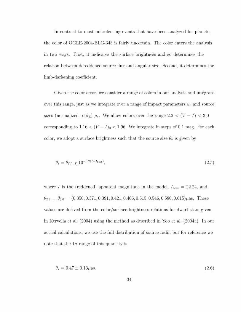
In contrast to most microlensing events that have been analyzed for planets,

the color of OGLE-2004-BLG-343 is fairly uncertain. The color enters the analysis

in two ways. First, it indicates the surface brightness and so determines the

relation between dereddened source flux and angular size. Second, it determines the

limb-darkening coefficient.

Given the color error, we consider a range of colors in our analysis and integrate

over this range, just as we integrate over a range of impact parameters u0 and source

sizes (normalized to θE) ρ∗. We allow colors over the range 2.2 < (V − I) < 3.0

corresponding to 1.16 < (V − I)0 < 1.96. We integrate in steps of 0.1 mag. For each

color, we adopt a surface brightness such that the source size θ∗ is given by

θ∗ = θ(V −I) 10−0.2(I−Ibest), (2.5)

where I is the (reddened) apparent magnitude in the model, Ibest = 22.24, and

θ2.2 . . . θ3.0 = (0.350, 0.371, 0.391, 0.421, 0.466, 0.515, 0.546, 0.580, 0.615)µas. These

values are derived from the color/surface-brightness relations for dwarf stars given

in Kervella et al. (2004) using the method as described in Yoo et al. (2004a). In our

actual calculations, we use the full distribution of source radii, but for reference we

note that the 1σ range of this quantity is

θ∗ = 0.47 ± 0.13µas. (2.6)

34

We find from the models of Claret (2000) and Hauschildt et al. (1999) that the

linear limb-darkening coefficients for dwarfs in our adopted color range vary by only

a few hundredths. Therefore, for simplicity, we adopt the mean of these values

ΓI = 0.50 (2.7)

for all colors. This corresponds to c = 3Γ/(2 + Γ) = 0.60 in the standard

limb-darkening parameterization (Afonso et al. 2000).

Finally, each model specifies not only a color and magnitude for the source, but

also a source distance. Evaluation of the likelihood of each specific combination of

these requires a color-magnitude relation. We adopt (Reid 1991)

MI = 2.37(V − I)0 + 2.89 (2.8)

with a scatter of 0.6 mag. The ridge of this relation is shown as a red line segment in

Figure 2.2, with the sources placed at 10−0.15/5R0 = 7.5 kpc and reddened according

to the red-clump determination, just as was done for the Hipparcos stars. This track

is in reasonable agreement with the Hipparcos stars.

2.3.3. Finite-Source Effects

Yoo et al. (2004b) define z0 ≡ u0/ρ∗ (where ρ∗ = θ∗/θE is the angular size

of the source θ∗ in units of θE), which is a useful parameter to characterize the

35

finite-source effects in single-lens microlensing events. We fit the observational data

to a set of point-lens models on a grid of (u0, z0) and then compare the resulting χ2

with the best-fit PSPL model. As mentioned in § 2.3.2, we adopt the limb-darkening

formalism of Yoo et al. (2004b) and for simplicity choose ΓI = 0.50.

Figure 2.4 displays the resulting ∆χ2 contours. It shows that the 1 σ contour

extends from z0 ≃ 0.2 to arbitrarily large z0. This is qualitatively similar to

OGLE-2003-BLG-423 as analyzed in Yoo et al. (2004b). However, as we demonstrate

in § 2.3.4, the range of z0 that is consistent with the Galactic model is quite different

for these two events. This is to be expected since z0 = u0/ρ∗ = (u0/θ∗)θE, and u0/θ∗

is roughly 8 times smaller for this event, while θE is generally of the same order.

Figure 2.4 shows contours for both Amax and u−10 . For z0 ≡ u0/ρ∗ > 2, these

are very similar, which is expected because in the absence of finite-source effects

(and for u0 ≪ 1), Amax = u−10 . Note that the Amax contours are roughly rectangular,

so that while z0 is not well constrained, the 3σ lower limit Amax > 103.16 ∼ 1450 is

quite well defined. This shows that although the blending is very severe, it is also

very well constrained, implying that the event’s high magnification is secure.

2.3.4. Monte-Carlo Simulation

We perform a similar Monte-Carlo simulation using a Han & Gould (1996, 2003)

model as described in Yoo et al. (2004b) by taking into account all combinations of

36

source and lens distances, Dl < Ds, uniformly sampled along the line of sight toward

the source (l, b) = (4.21,−3.47). The simulation adopts the Gould (2000a) mass

function taking into account the bulge main sequence stars, white dwarfs (distributed

around 0.6 M⊙), neutron stars (narrowly peaked at 1.35 M⊙), and stellar-mass black

holes. This mass function is adequate to describe mass distributions of disk lenses

except that the disk contains stars with masses greater than 1 M⊙ while the bulge

does not. However, a disk main sequence star more massive than the Sun will be

too bright to be the lens star for this event (see Fig. 2.2); so for simplicity, we use

this mass function for both disk and bulge in our simulation. In Yoo et al. (2004b),

the source flux is determined from the tE for each Monte-Carlo event since only the

PSPL model is considered at this step. However, when finite-source effects are taken

into account, each tE corresponds to a series of Fs depending on the source size ρ∗,

so there is no longer a 1-1 correspondence between Fs and tE. As discussed in Yoo

et al. (2004a), θ∗ can be deduced from the source’s dereddened color and magnitude.

Since θE is known for each simulated event, ρ∗ is a direct function of Fs and the

(V − I) color of the source,

ρ∗ =θ(V −I)

θE

√

Fs

Fbest

, (2.9)

where Fbest corresponds to Ibest in equation (2.5). Using this constraint, we fit the

k-th Monte-Carlo event to a point-lens model with finite-source effects, holding tE,k

fixed at the value given by the simulation, for a variety of (V − I) color values

37

inferred from § 2.3.2. Hence, for the j-th (V − I) color and k-th Monte-Carlo

event, we have best-fit single-lens light-curve parameters t0,j,k, u0,j,k, ρ∗,j,k, Fs,j,k,

Fb,j,k, as well as ∆χ2j,k ≡ χ2

j,k − χ2PSPL. We construct a three-dimensional table that

includes these six quantities as well as the other parameters from the Monte-Carlo

simulation (tE,k, θE,k, Ds,k, Dl,k, Ml,k, Γk), the Einstein timescale and radius, the

source and lens distances, the lens mass, and the event rate. From these can also

be derived two other important quantities, the source absolute magnitude MI,j,k

and the physical Einstein radius rE,k ≡ θE,k × Dl,k. This three-dimensional table

is composed of nine two-dimensional tables, one for each (V − I)j color. Each

table contains approximately 200,000 rows, one for each simulated event. To make

the notation more compact, we refer to the parameters a, b, c, ... lying in the bin

a ∈ [amin, amax]; b ∈ [bmin, bmax]; c ∈ [cmin, cmax]... as bin(a, b, c, ...).

Similarly to Yoo et al. (2004b), the posterior probability of ai lying in bin(ai) is

given by

P [bin(ai)] ∝∑

j,k

(PV −I)j × (PReid)j,k × exp[−∆χ2j,k/2] (2.10)

×BC[bin(aij,k)] × Γk,

where (PReid)j,k = exp(−(MI)j,k −MI,Reid[(V − I)0,j]2/2[σ2Reid + (σMI

)2j,k]) accounts

for the scatter (σReid = 0.6) in MI about the Reid relation plus the dispersion

(σMI)j,k from light-curve fitting, (PV −I)j = exp−[(V − I)j − (V − I)best]

2/2σ2(V −I)

38

reflects the uncertainty in V − I color, and BC is a boxcar function defined by

BC[bin(a)] ≡ Θ (a − amin) × Θ (amax − a).

Figure 2.5 shows the posterior probability distributions of various parameters,

including u0, dereddened apparent I-band magnitude of the source I0, proper motion

µ, z0, source distance modulus, lens distance modulus, absolute I-band magnitude

of the source MI , and lens mass. The blue and red histograms represent bulge-disk

events and bulge-bulge events, respectively. The relative event rate is normalized

in the same way for both bulge-disk and bulge-bulge events. The total rate for

bulge-disk events is about 6 times larger than that for bulge-bulge events, which

means that the Monte-Carlo simulation tends strongly to favor bulge-disk events.

The Einstein radii are on average smaller for bulge-bulge events than for

bulge-disk events, and as a result, the bulge-bulge events tend to have bigger ρ∗

and hence smaller z0. However, the top right panel of Figure 2.5 shows that the z0

probability distributions have similar shapes for both bulge-bulge and bulge-disk

events. This is because the (lack of) finite-source effects constrain z0 ∼> 0.7 at

the 3σ level (see Fig. 2.4), which cuts off the lower end of the z0 distributions for

both categories of events. Since bulge-disk events have smaller ρ∗ than bulge-bulge

events, the u0 posterior probability distribution peaks at a lower value for the

former. Furthermore, since z0 ∼> 0.7, the proper motion is constrained to be

µ = θ∗z0/teff ∼> 7mas/yr, which is typical of bulge-disk events but ∼> 2 times the

proper motion of typical bulge-bulge events.

39

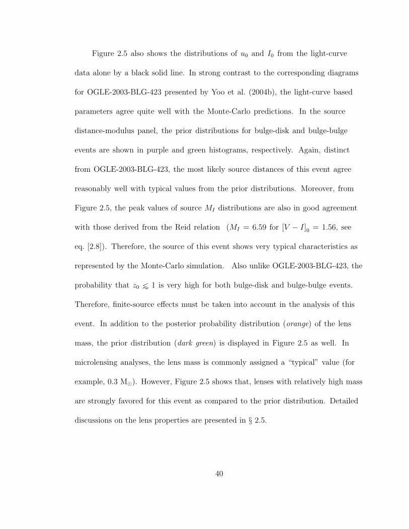
Figure 2.5 also shows the distributions of u0 and I0 from the light-curve

data alone by a black solid line. In strong contrast to the corresponding diagrams

for OGLE-2003-BLG-423 presented by Yoo et al. (2004b), the light-curve based

parameters agree quite well with the Monte-Carlo predictions. In the source

distance-modulus panel, the prior distributions for bulge-disk and bulge-bulge

events are shown in purple and green histograms, respectively. Again, distinct

from OGLE-2003-BLG-423, the most likely source distances of this event agree

reasonably well with typical values from the prior distributions. Moreover, from

Figure 2.5, the peak values of source MI distributions are also in good agreement

with those derived from the Reid relation (MI = 6.59 for [V − I]0 = 1.56, see

eq. [2.8]). Therefore, the source of this event shows very typical characteristics as

represented by the Monte-Carlo simulation. Also unlike OGLE-2003-BLG-423, the

probability that z0 ∼< 1 is very high for both bulge-disk and bulge-bulge events.

Therefore, finite-source effects must be taken into account in the analysis of this

event. In addition to the posterior probability distribution (orange) of the lens

mass, the prior distribution (dark green) is displayed in Figure 2.5 as well. In

microlensing analyses, the lens mass is commonly assigned a “typical” value (for

example, 0.3 M⊙). However, Figure 2.5 shows that, lenses with relatively high mass

are strongly favored for this event as compared to the prior distribution. Detailed

discussions on the lens properties are presented in § 2.5.

40

2.4. Detecting Planets

While there are no obvious deviations from point-lens behavior in the light

curve of OGLE-2004-BLG-343 at our adopted threshold of ∆χ2min = 60, planetary

deviations might be difficult to recognize by eye. We must therefore conduct a

systematic search for such deviations. Logically, this search should precede the

second step of testing to determine what planets we could have detected had they

been there. However, as a practical matter it makes more sense to first determine

the range of parameter space for which we are sensitive to planets because it is

only this range that needs to be searched for planets. We therefore begin with this

detection efficiency calculation.

2.4.1. Detection Efficiency

As reviewed in § 2.1.2, a variety of methods have been proposed to calculate

the planetary sensitivities of microlensing events, either in predicting planetary

detection efficiencies theoretically or in analyzing real observational data sets. In

those methods, ∆χ2 is often calculated by subtracting the χ2 of single-lens models

from that of the binary-lens models to evaluate detection sensitivities. However,

the ways in which single-lens and binary-lens models are compared differ from

study to study. As noted by Griest & Safizadeh (1998) and Gaudi & Sackett

(2000), for real planetary light curves, the lens parameters are not known a priori.

41

Therefore, ∆χ2 will generally be exaggerated if one subtracts from the binary lens

model the single-lens model that has the same t0, u0, and tE instead of the best-fit

single-lens model to the binary light curve. One important factor contributing to this

exaggeration is that the center of the magnification pattern (referred to as the center

of the caustic in Yoo et al. 2004b) in the binary-lens case is no longer the position of

the primary star as it is in the single-lens model (Dominik 1999b; An & Han 2002).

Therefore light-curve parameters such as u0 and t0 will shift correspondingly. We

find that by not taking into account this effect and directly comparing the simulated

binary (i.e., planetary) light curve with the best-fit single-lens model to the data,

Abe et al. (2004) exaggerate the planetary sensitivity of MOA 2003-BLG-32/OGLE

2003-BLG-219, although it remains the most sensitive event analyzed to date (see

Appendix B).

Following Gaudi & Sackett (2000), planetary systems are characterized by

a planet-star mass ratio q, planet-star separation in Einstein radius b, and the

angle α of the source trajectory relative to the planet-star axis. In our binary-lens

calculations, u0 and t0 are defined with respect to the center of magnification

discussed above. According to Gaudi & Sackett (2000), the next step is to fit the

data to both PSPL models and binary-lens models with a variety of (b, q, α) and

calculate ∆χ2(b, q, α) = χ2(b, q, α) − χ2PSPL. Then ∆χ2(b, q, α) is compared with a

threshold value χ2thres: if ∆χ2 > χ2

thres then a planet with parameters b, q, and α is

claimed to be excluded while it is detected if ∆χ2 < −χ2thres. The (b, q) detection

42

efficiency is then obtained by integrating Θ(∆χ2 − ∆χ2thres) over α in the exclusion

region at fixed (b, q), where Θ is a step function. However, Gaudi et al. (2002)

point out that for events with poorly constrained light-curve parameters, which is

the case for OGLE-2004-BLG-343, this method will significantly underestimate the

sensitivities since the binary-lens models will minimize the χ2 over the relatively

large available parameter space. As discussed in Yoo et al. (2004b), the detection

efficiency should be evaluated at a series of allowed u0 values. To take finite-source

effects into account, we generate a grid of permitted (u0, ρ∗), and each (u0,m, ρ∗,m) bin

is associated with the probability P [bin(u0,m, ρ∗,m)] obtained using the following

equation:

P [bin(u0,m, ρ∗,m)] ∝∑

j,k

Pm,j,k (2.11)

where

Pm,j,k = (PV −I)j × (PReid)j,k × exp[−∆χ2j,k/2] × BC[bin(u0,mj,k)]

×BC[bin(ρ∗,mj,k)] × Γk (2.12)

If the light-curve parameters were well-constrained, the approaches of Gaudi

& Sackett (2000) and Rhie et al. (2000) would be very nearly equivalent, with the

former retaining a modest philosophical advantage, since it uses only the observed

light curve and does not require construction of light curves for hypothetical events.

43

However, because in our case these parameters are not well constrained, the Gaudi

& Sackett (2000) approach would require integration over all binary-lens parameters

(except Fs and Fb). Regardless of its possible philosophical advantages, this approach

is therefore computationally prohibitive in the present case. We therefore do not

follow Gaudi & Sackett (2000), but instead construct a binary light curve with the

same observational time sequence and photometric errors as the OGLE observations

of OGLE-2004-BLG-343, for each (b, q, α ; u0, ρ∗) combination and the associated

probability-weighted parameters alc: t0, tE, Fs and Fb in the m-th (u0, ρ∗) bin,

alc(weighted),m =

∑

j,kPm,j,kalc,j,k

∑

j,kPm,j,k

. (2.13)

Then each simulated binary light curve (b, q, α ; u0,m, ρ∗,m) is fitted to a

single-lens model with finite-source effects whose best fit yields χ2(b, q, α ; u0,m, ρ∗,m).

Another set of artificial binary light curves is generated under the assumption

that OGLE had triggered a dense series of observations following the internal

alert at HJD′ 3175.54508. These cover the peak of the event with the normal

OGLE frequency and are used to compare results with those obtained from the real

observations.

Magnification calculations for a binary lens with finite-source effects are very

time-consuming. Besides (b, q, α), our calculations are also performed on (u0, ρ∗)

grids, two more dimensions than in any previous search of a grid of models with

finite-source effects included. This makes our computations extremely expensive,

44

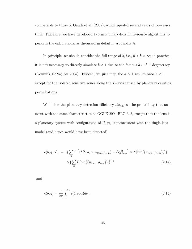
comparable to those of Gaudi et al. (2002), which equaled several years of processor

time. Therefore, we have developed two new binary-lens finite-source algorithms to

perform the calculations, as discussed in detail in Appendix A.

In principle, we should consider the full range of b, i.e., 0 < b < ∞; in practice,

it is not necessary to directly simulate b < 1 due to the famous b ↔ b−1 degeneracy

(Dominik 1999a; An 2005). Instead, we just map the b > 1 results onto b < 1

except for the isolated sensitive zones along the x−axis caused by planetary caustics

perturbations.

We define the planetary detection efficiency ǫ(b, q) as the probability that an

event with the same characteristics as OGLE-2004-BLG-343, except that the lens is

a planetary system with configuration of (b, q), is inconsistent with the single-lens

model (and hence would have been detected),

ǫ(b, q, α) = ∑

m

Θ[

χ2(b, q, α ; u0,m, ρ∗,m) − ∆χ2thres

]

× P [bin(u0,m, ρ∗,m)]

×∑

m

P [bin(u0,m, ρ∗,m)]−1 (2.14)

and

ǫ(b, q) =1

2π

∫ 2π

0ǫ(b, q, α)dα. (2.15)

45

2.4.2. Constraints on Planets

Figure 2.6 shows the planetary detection efficiency of OGLE-2004-BLG-343

for planets with mass ratios q = 10−3, 10−4, and 10−5, as a function of b, the

planet-star separation (normalized to θE), and α, the angle that the moving source

makes with the binary axis passing the primary lens star on its left. Different colors

indicate 10%, 25%, 50%, 75%, 90% and 100% efficiency. Note that the contours are

elongated along an axis that is roughly 60 from the vertical (i.e., the direction of

the impact parameter for α = 0). This reflects the fact that the point closest to

the peak occurs at t = 2453175.77626 when (t − t0)/tE = 2.16u0, and so when the

source-lens separation is at an angle tan−1 2.16 = 65. For q = 10−3, the region

of 100% efficiency extends through 360 within about one octave on either side of

the Einstein ring. However, at lower mass ratios there is 100% efficiency only in

restricted areas close to the Einstein ring and along the above-mentioned principal

axis.

Figure 2.7 summarizes an ensemble of all figures similar to Figure 2.6, but with

q ranging from 10−2.5 to 10−5.0 in 0.1 increments. To place this summary in a single

figure, we integrate over all angles α at fixed b. Comparison of this figure to Figure 8

from Gaudi et al. (2002) shows that the detection efficiency of OGLE-2004-BLG-343

is similar to that of MACHO-1998-BLG-35 and OGLE-1999-BUL-35 despite the fact

that their maximum magnifications are Amax ∼ 100, roughly 30 times lower than

46

OGLE-2004-BLG-343. Of course, part of the reason is that OGLE-2004-BLG-343

did not actually probe as close as u = u0 ∼ 1/3000 because no observations were

taken near the peak. However, observations were made at u ∼ 1/1200, about 12

times closer than in either of the two events analyzed by Gaudi et al. (2002). One

problem is that because the peak was not well covered, there are planet locations

that do not give rise to observed perturbations at all. But this fact only accounts for

the anisotropies seen in Figure 2.6. More fundamentally, even perturbations that do

occur in the regions that are sampled by the data can often be fitted to a point-lens

light curve by “adjusting” the portions of the light curve that are not sampled.

Note the central “spike” of reduced detection efficiency plots near b = 1. As

first pointed out by Bennett & Rhie (1996), this is due to the extreme weakness of

the caustic for nearly resonant (b ∼ 1) small mass-ratio (q ≪ 1) binary lenses.

2.4.3. No Planet Detected

Based on the detection efficiency levels we obtained in § 2.4.2, we fit the

observational data to binary-lens models to search for a planetary signal in the

regions with efficiency greater than zero from q = 10−5 to q = 10−2.5. We find

no binary-lens models satisfying our detection criteria. In fact, the total χ2

contributions to the best-fit single-lens model of the observational points over the

peak ( HJD = 2453175.5 − 2453176.0) are no more than 30, so even if all of these

47

deviations were due to a planetary perturbation, such a binary-lens solution would

not easily satisfy our ∆χ2 = 60 detection criteria. Therefore there are no planet

detections in OGLE-2004-BLG-343 data.

2.4.4. Fake Data

Partly to explore further the issue of imperfect coverage of the peak, and partly

to understand how well present microlensing experiments can probe for planets, we

now ask what would have been the detection efficiency of OGLE-2004-BLG-343 if

the internal alert issued on HJD′ 3175.54508 had been acted upon.

Of course, since the peak was not covered, we do not know exactly what u0

and ρ for this event are. However, for purposes of this exercise, we assume that they

are near the best fit as determined from a combination of the light-curve fitting and

the Galactic Monte Carlo, and for simplicity, we choose u0 = 0.00040, ρ∗ = 0.00040

which is very close to the best-fit combination. We then form a fake light curve

sampled at intervals of 4.3 minutes, starting from the alert and continuing to the

end of the actual observations that night. This sampling reflects the intense rate

of OGLE follow-up observations actually achieved during this event (see § 2.2). We

assume errors similar to those of the actual OGLE data at similar magnifications.

For those points that are brighter than the brightest OGLE point, the minimum

actual photometric errors are assigned. We also assume that the color information is

48

known exactly in this case to be V − I = 2.6. We then analyze these fake data in

exactly the same way that we analyze the real data. In contrast to the real data,

however, we do not find a finite range of z0 ≡ u0/ρ∗ that are consistent with the fake

data. Rather, we find that all consistent parameter combinations have z0 = 1 almost

identically. We therefore consider only a one-dimensional set of (u0, ρ∗) combinations

subject to this constraint.

Figure 2.8 is analogous to Figure 2.6 except that the panels show planet

sensitivities for q = 10−3, 10−4, 10−5, and 10−6, that is, an extra decade. In sharp

contrast to the real data, these sensitivities are basically symmetric in α, except for

the lowest value of q. Sensitivities at all mass ratios are dramatically improved.

For example, at q = 10−3, there is 100% detection efficiency over 1.7 dex in b

(1/7 ∼< b ∼< 7). Even at q = 10−5 (corresponding to an Earth-mass planet around an

M star), there is 100% efficiency over an octave about the Einstein radius.

Figure 2.9 is the fake-data analog of Figure 2.7. It shows that this event would

have been sensitive to extremely low mass-ratios, lower than those accessible to any

other technique other than pulsar timing.

2.4.5. Detection Efficiency in Physical Parameter Space

One of the advantages of the Monte Carlo approach of Yoo et al. (2004b) is

that it permits one to evaluate the planetary detection efficiency in the space of

49

the physical parameters, planet mass and projected physical separation (mp, r⊥),

rather than just the microlensing parameters (b, q). Figures 2.10 and 2.11 show

this detection efficiency for the real and fake data, respectively. The fraction

of Jupiter-mass planets that could have been detected from the actual data

stream is greater than 25% for 0.8AU ∼< r⊥ ∼< 10AU and is greater than 90% for

2AU ∼< r⊥ ∼< 6AU. There is also marginal sensitivity to Neptune-mass planets.

However, the detection efficiencies would have been significantly enhanced had the

FWHM around the peak been observed, as previously discussed by Rattenbury et

al. (2002). For the fake data, more than 90% of Jupiter-mass planets in the range

0.7AU ∼< r⊥ ∼< 20AU and more than 25% with 0.3AU ∼< r⊥ ∼< 30AU would have

been detected. Indeed, some sensitivity would have extended all the way down to

Earth-mass planets.

2.5. Luminous Lens?

Understanding the physical properties of their host stars is a major component

of the study of extra-solar planets. It is especially important to know the mass and

distance of the lens star for planets detected by microlensing because only then

can we accurately determine the planet’s mass and physical separation from the

star. Obtaining similar information for microlensing events that are unsuccessfully

searched for planets enables more precise estimates of the detection efficiency. There

50

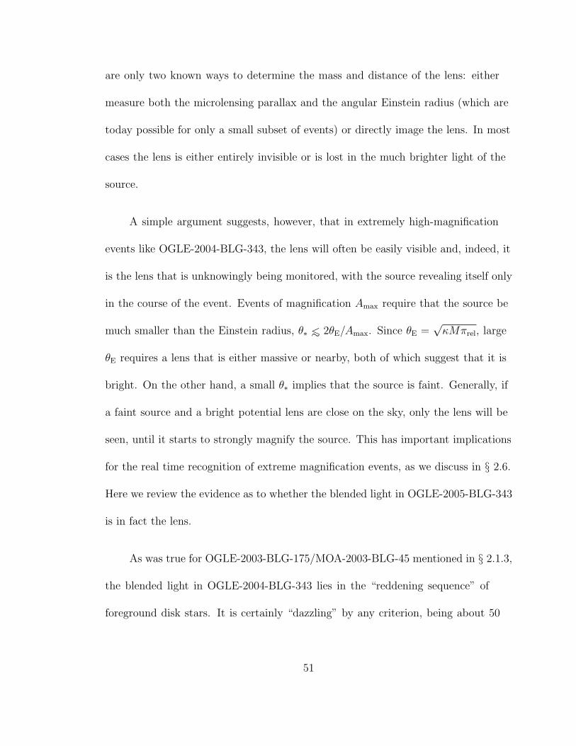
are only two known ways to determine the mass and distance of the lens: either

measure both the microlensing parallax and the angular Einstein radius (which are

today possible for only a small subset of events) or directly image the lens. In most

cases the lens is either entirely invisible or is lost in the much brighter light of the

source.

A simple argument suggests, however, that in extremely high-magnification

events like OGLE-2004-BLG-343, the lens will often be easily visible and, indeed, it

is the lens that is unknowingly being monitored, with the source revealing itself only

in the course of the event. Events of magnification Amax require that the source be

much smaller than the Einstein radius, θ∗ ∼< 2θE/Amax. Since θE =√

κMπrel, large

θE requires a lens that is either massive or nearby, both of which suggest that it is

bright. On the other hand, a small θ∗ implies that the source is faint. Generally, if

a faint source and a bright potential lens are close on the sky, only the lens will be

seen, until it starts to strongly magnify the source. This has important implications

for the real time recognition of extreme magnification events, as we discuss in § 2.6.

Here we review the evidence as to whether the blended light in OGLE-2005-BLG-343

is in fact the lens.

As was true for OGLE-2003-BLG-175/MOA-2003-BLG-45 mentioned in § 2.1.3,

the blended light in OGLE-2004-BLG-343 lies in the “reddening sequence” of

foreground disk stars. It is certainly “dazzling” by any criterion, being about 50

51

times brighter than the source in I and 150 times brighter in V (see Fig. 2.2). Is the

blended light also due to the lens in this case?

There is one argument for this hypothesis and another against. We initiate

the first by estimating the mass and distance to the blend as follows. We

model the extinction due to dust at a distance x along the line of sight by

dAI/dx = 0.4 kpc−1e−qx and set q = 0.26 kpc−1 in order to reproduce the measured

extinction to the bulge AI(8 kpc) = 1.34. Using the Reid (1991) color-magnitude

relation, we then adjust the distance to the blend until it reproduces the observed

color and magnitude of the blend. We find a distance modulus of 12.6 (∼ 3.3 kpc),

and with the aid of the Cox (2000) mass-luminosity relation, we estimate a

corresponding mass Ml = 0.9 M⊙. Inspecting Figure 2.5, we see that this is almost

exactly the peak of the lens-distance distribution function predicted by combining

light-curve information and the Galactic model. This is quite striking because, in the

absence of light-curve information, the lens would be expected to be relatively close

to the source. From our Monte-Carlo simulation toward the line of sight of this

event, the total prior probability of the bulge-bulge events is about 1.5 times higher

than the prior probability of the bulge-disk events, and furthermore, only about 7%

of all events have lenses less than 3.3 kpc away (see green and purple histograms in

source and lens distance modulus panels of Fig. 2.5). It is only because the light

curve lacks obvious finite-source effects (despite its very high-magnification) that one

is forced to consider lenses with large θE, which generally drives one toward nearby

52

lenses in the foreground disk. Based on our experience analyzing many blended

microlensing events, the blended light is most often from a bulge star rather than

a disk star, which simply reflects the higher density of bulge stars. In brief, it is

quite unusual for lenses to be constrained to lie in the disk, and it is quite unusual

for events to be blended with foreground disk stars. This doubly unusual set of

circumstances would be more easily explained if the blend were the lens.

However, if the blend were the lens, then the source and lens would be aligned

to better than 1 mas during the event, and one would therefore expect that the

apparent position of the source would not change as the source first brightened

and then faded. In fact, we find that the apparent position does change by about

73 ± 9 mas. However, since the apparent source (i.e., combined source and blended

light at baseline) has a near neighbor at 830 mas, which is almost as bright as the

source/blend, it is quite possible that the lens actually is the blend, but that this

neighbor is corrupting the astrometry.

Thus, the issue cannot be definitively settled at present. However, it could be

resolved in principle by, for example, obtaining high-resolution images of the field a

decade after the event when the source and lens have separated sufficiently to both

be seen. If the blend is the lens, then they will be seen moving directly apart with

a proper motion given µ = θE/tE, where θE is derived from the estimated mass and

distance to the lens and tE is the event timescale.

53

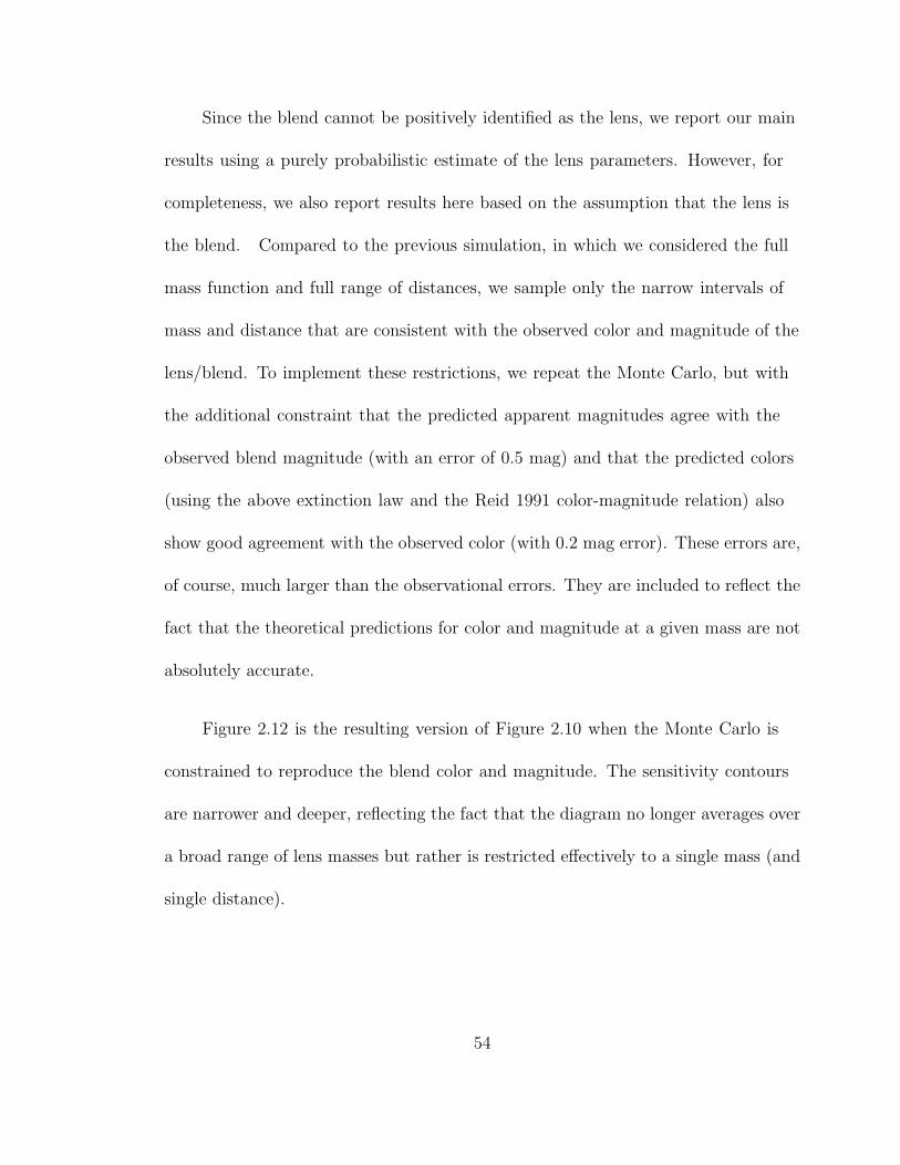
Since the blend cannot be positively identified as the lens, we report our main

results using a purely probabilistic estimate of the lens parameters. However, for

completeness, we also report results here based on the assumption that the lens is

the blend. Compared to the previous simulation, in which we considered the full

mass function and full range of distances, we sample only the narrow intervals of

mass and distance that are consistent with the observed color and magnitude of the

lens/blend. To implement these restrictions, we repeat the Monte Carlo, but with

the additional constraint that the predicted apparent magnitudes agree with the

observed blend magnitude (with an error of 0.5 mag) and that the predicted colors

(using the above extinction law and the Reid 1991 color-magnitude relation) also

show good agreement with the observed color (with 0.2 mag error). These errors are,

of course, much larger than the observational errors. They are included to reflect the

fact that the theoretical predictions for color and magnitude at a given mass are not

absolutely accurate.

Figure 2.12 is the resulting version of Figure 2.10 when the Monte Carlo is

constrained to reproduce the blend color and magnitude. The sensitivity contours

are narrower and deeper, reflecting the fact that the diagram no longer averages over

a broad range of lens masses but rather is restricted effectively to a single mass (and

single distance).

54

2.6. Summary and Discussion

In this paper we present our analysis of microlensing event OGLE-2004-BLG-

343, with the highest peak magnification (Amax = 3000±1100) ever analyzed to date.

The light curve is consistent with the single-lens microlensing model, and no planet

has been detected in this event. We demonstrate that if the peak had been well

covered by the observations, the event would have had the best sensitivity to planets

to date, and it would even have had some sensitivity to Earth-mass planets (§ 2.4.4,

§ 2.4.5). However, this potential has not been fully realized due to human error

(§ 2.2), and OGLE-2004-BLG-343 turns out to be no more sensitive to planets than

a few other high-magnification events analyzed before (§ 2.4.2, § 2.4.5). Thus, while

ground-based microlensing surveys are technically sufficient to detect very low-mass

planets, the relatively short timescale of the sensitive regime of high-magnification

microlensing events demands a rapidity of response that is not consistently being

achieved. In the final paragraph below, we develop several suggestions to rectify this

situation.

In § 2.3 we show that finite-source effects are important in analyzing this

event, so we extend the method of Yoo et al. (2004b) to incorporate such effects in

planetary detection efficiency analysis. Moreover, since magnification calculations

of binary-lens models with finite-source effects are computationally remarkably

expensive, and applying previous finite-source algorithms, it would have taken

55

of order a year of CPU time to do the detection efficiency calculation required

by this event. We therefore develop two new binary-lens finite-source algorithms

(Appendix A) that are considerably more efficient than previous ones. The

“map-making” method (Appendix A.1) is an improvement on the conventional

inverse ray-shooting method, which proves to be especially efficient for use in

detection efficiency calculations, while the “loop-linking” method (Appendix A.2)

is more versatile and could be easily implemented in programs aimed at finding

best-fit finite-source binary-lens solutions. Using these algorithms, we were able to

complete the computations for this paper in about 4 processor-weeks, roughly an

order of magnitude faster than would have been required using previous algorithms.

Finally, we show in § 2.5 that the blend, which is a Galactic disk star, might

very possibly be the lens, and that this case also proves to be highly probable

from the Monte-Carlo simulation. However, it seems to contradict the astrometric

evidence, and we point out that this issue could in principle be solved by future

high-resolution images. Among the high-magnification events discovered by current

microlensing survey groups, it is very likely that the lens star, which is also the

apparent source, of those events is in the Galactic disk. Thus the blended light

is usually far brighter than the source, thereby increasing the difficulty in early

identification of such events. This fact motivates the first of several suggestions

aimed at improving the recognition of very high-magnification events:

56

1) When events are initially alerted they should be accompanied by instrumental

CMD of the surrounding field, with the location of the apparent “source”

highlighted. Events whose apparent sources lie on the “reddening sequence”

of foreground disk stars (see Fig. 2.2) have a high probability to actually be

lenses of more distant (and fainter) bulge sources. These events deserve special

attention even if their initial light curves appear prosaic.

2) For each such event it is possible to measure the color (but not immediately

the magnitude) of the source by the standard technique of obtaining two-band

photometry and measuring the slope of the relative fluxes in the two bands.

If the color is different from that of the apparent “source” at baseline, that

will prove that this baseline light is not primarily due to the source, and it will

increase the probability that this baseline object is the lens. Moreover, if the

source color is relatively red, it will show that the source is probably faint and

so is (1) most likely already fairly highly magnified (thereby making it possible

to detect above the foreground blended light) and (2) capable, potentially at

least, of being magnified to very high magnification (see § 2.5). This would

motivate obtaining more data while the event was still faint to help predict

its future behavior and would enable a guess as to how to “renormalize” the

event’s apparent magnification to its true magnification. This is important

because generally one cannot accurately determine this renormalization until

57

the event is within 0.4 mag (when the event is teff before its peak), at which

point it may well be too late to act on this knowledge.

3) Both survey groups and follow-up groups should issue alerts on suspected

high-magnification events guided by a relatively low threshold of confidence,

recognizing that this will lead to more “false alerts” than at present. If such

alerts are accompanied by a cautionary note, they will promote intergroup

discussions that could lead to more rapid identification of high-magnification

events without compromising the credibility of the group.

58

Fig. 2.1.— Light curve of OGLE-2004-BLG-343 near its peak on 2004 June 19(HJD 2,453,175.7467). Only OGLE I-band data (open circles) are u sed in mostof the analysis, except OGLE V -band data (open triangles) and µFUN H-band data(crosses) are used to constrain the color of the source star. All bands are linearlyrescaled so that Fs and Fb are the same as the OGLE I-band observations. The solidline shows the bes t-fit PSPL model. The upper right inset shows the peak of thelight curve, wit h the range of the simulated data points plotted by the thick line.

59

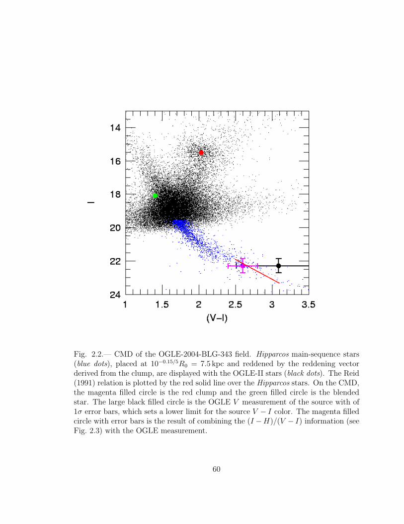
Fig. 2.2.— CMD of the OGLE-2004-BLG-343 field. Hipparcos main-sequence stars(blue dots), placed at 10−0.15/5R0 = 7.5 kpc and reddened by the reddening vectorderived from the clump, are displayed with the OGLE-II stars (black dots). The Reid(1991) relation is plotted by the red solid line over the Hipparcos stars. On the CMD,the magenta filled circle is the red clump and the green filled circle is the blendedstar. The large black filled circle is the OGLE V measurement of the source with of1σ error bars, which sets a lower limit for the source V − I color. The magenta filledcircle with error bars is the result of combining the (I −H)/(V − I) information (seeFig. 2.3) with the OGLE measurement.

60

Fig. 2.3.— (VOGLE − IOGLE)/(IOGLE − H2MASS) color-color diagram. All points arefrom matching 2MASS H-band data with OGLE-II V, I photometry in a field centeredon OGLE-2004-BLG-343. Stars on the giant branch are shown by open circles. Thesolid and dashed vertical lines represent the source IOGLE−H2MASS color transformedfrom its IOGLE−HµFUN value and its 1σ ranges. Their intersections with the diagonaltrack of stars give corresponding VOGLE − IOGLE colors, which are represented by thehorizontal lines.

61

Fig. 2.4.— Likelihood contours (1σ, 2σ, 3σ) for finite-source points-lens modelsrelative to the best-fit PSPL model. Contours with x-axis as log u−1

0 and log Amax

are displayed in solid and dashed lines, respectively.

62

b-b(posterior)b-d(posterior)

bigger finite-sourceeffects

b-b(prior)b-d(prior)

priorposterior

Fig. 2.5.— Probability distributions of u0, dereddened apparent I-band magnitudeof the source I0, proper motion µ, log(z0), source distance modulus, lens distancemodulus, absolute I-band magnitude of the source MI , and lens mass for Monte Carloevents toward the line of sight of OGLE-2004-BLG-343. Blue histograms representthe posterior probability distributions for bulge-disk microlensing events while redones represent the posterior probability distributions for bulge-bulge events. In thesource and lens distance-modulus panels, histograms in purple and green representthe prior probability distributions for bulge-disk and bulge-bulge events, respectively.The black Gaussian curves in the u0 and I0 panels show probability distributions fromPSPL light-curve fitting alone. In the lens mass panel, the dark green histogram showsthe prior probability distribution, while the orange histogram represents the posteriordistribution.

63

Fig. 2.6.— (For real data) Planetary detection efficiency for mass ratios q = 10−3,10−4, and 10−5 for OGLE-2004-BLG-343 as a function of the planet-star separationbx = b× cos α and by = b× sin α in the units of θE where α is the angle of planet-staraxis relative to the source-lens direction of motion. Different colors indicate 10% (red),25% (yellow), 50% (green), 75% (cyan), 90% (blue) and 100% (magenta) efficiency.The black circle is the Einstein ring, i.e., b = 1.

64

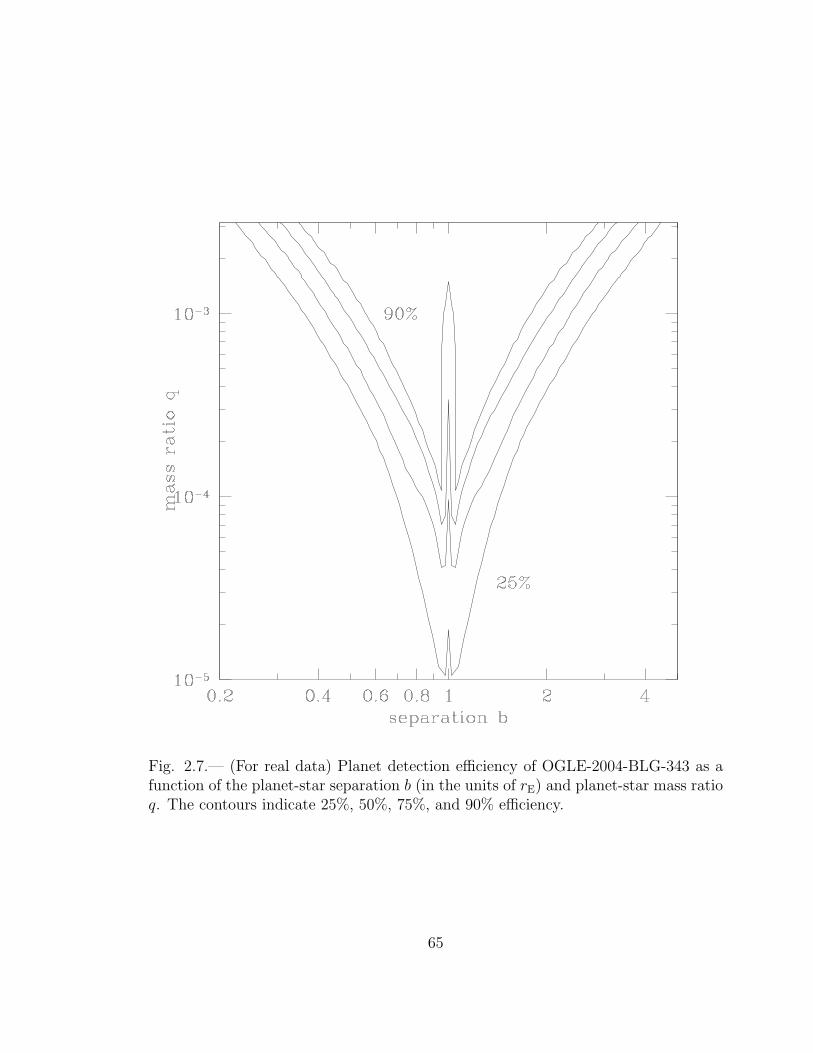
Fig. 2.7.— (For real data) Planet detection efficiency of OGLE-2004-BLG-343 as afunction of the planet-star separation b (in the units of rE) and planet-star mass ratioq. The contours indicate 25%, 50%, 75%, and 90% efficiency.

65

Fig. 2.8.— (For fake data) Planetary detection efficiency for mass ratios q = 10−3,10−4, 10−5 and 10−6 of OGLE-2004-BLG-343 augmented by simulated data pointscovering the peak as a function of the planet-star separation bx and by in the units ofθE. Different colors indicate 10% (red), 25% (yellow), 50% (green), 75% (cyan), 90%(blue) and 100% (magenta) efficiency. The black circle is the Einstein ring, i.e., b = 1.

66

Fig. 2.9.— (For fake data) Planetary detection efficiency of OGLE-2004-BLG-343augmented by simulated data points covering the peak. as a function of the planet-star separation b (in the units of θE) and planet-star mass ratio q. The contoursrepresent 25%, 50%, 75%, and 90% efficiency.

67

Fig. 2.10.— (For real data) Planetary detection efficiency as a function of r⊥, thephysical projected star-planet distance and mp, the planetary mass for OGLE-2004-BLG-343. The contours represent 25%, 50%, 75%, and 90% efficiency.

68

Fig. 2.11.— (For fake data) Planetary detection efficiency as a function of r⊥,the physical projected star-planet distance and mp, the planetary mass for OGLE-2004-BLG-343 augmented by simulated data points covering the peak. The contoursrepresent 25%, 50%, 75%, and 90% efficiency.

69

Fig. 2.12.— Planetary detection efficiency as a function of r⊥, the physical projectedstar-planet distance, and mp, the planetary mass for OGLE-2004-BLG-343, byassuming that the blended light is due to the lens. The contours represent 25%,50%, 75%, and 90% efficiency.

70

t0(HJD’) u0 tE(days) Is Ib χ2 Degree of Freedom

3175.7467 ± 0.0005 0.000333 ± 0.000121 42.5 ± 15.6 22.24 ± 0.40 18.08 ± 0.01 200.1 188

Table 2.1. OGLE-2004-BLG-343 Best-Fit PSPL Model Parameters

71

Chapter 3

Microlensing Event MOA-2007-BLG-400:

Exhuming the Buried Signature of a Cool,

Jovian-Mass Planet

3.1. Introduction

In the currently favored paradigm of planet formation, the location of the snow

line in the protoplanetary disk plays a pivotal role. Beyond the snow line, ices can

condense, and the surface density of solids is expected to be higher by a factor of

several relative to its value just inside this line. As a result of this increased surface

density, planet formation is expected to be most efficient just beyond the snow

line, whereas for increasing distances from the central star the planet formation

efficiency drops, as the surface density decreases and the dynamical time increases

(Lissauer 1987). In this scenario, gas-giant planets must form in the region of the

protoplanetary disk immediately beyond the snow-line, as the higher surface density

is required to build icy protoplanetary cores that are sufficiently massive to accrete

a substantial gaseous envelope while there is remaining nebular gas (Pollack et al.

1996). Low-mass primaries are expected to be much less efficient at forming gas

72

giants because of the longer dynamical times and lower surface densities at the snow

lines of these stars (Laughlin et al. 2004; Ida & Lin 2005; Kennedy & Kenyon 2008).

Migration due to nebular tides and other dynamical processes can then bring the icy

cores or gas giants from their formation sites to orbits substantially interior to the

snow line (Lin et al. 1996; Ward 1997; Rasio & Ford 1996).

The precise location of the snow line in protoplanetary disks is a matter of

some debate (e.g., Lecar et al. 2006), and is even likely to evolve during the epoch

of planet formation, particularly for low-mass stars (Kennedy et al. 2006; Kennedy

& Kenyon 2008). The condensation temperature of water is ∼ 170 K, and a fiducial

value for the location of the snow line in solar-mass stars motivated by observations

in our solar system is ∼ 2.7 AU. This may scale linearly with the stellar mass M ,

since the stellar luminosity during the epoch of planet formation scales as ∼ M2

for stars with M ∼< M⊙ (Burrows et al. 1993, 1997). Whereas the radial velocity

and especially transit methods are most sensitive to planets that are close to their

parent star at distances well inside the snow line, the sensitivity of the microlensing

method peaks at planetary separations near the Einstein ring radius of the primary

lens (Mao & Paczynski 1991; Gould & Loeb 1992), which is ∼ 3.5 AU(M/M⊙)1/2 for

typical lens and source distances of 6 kpc and 8 kpc, respectively. This corresponds

to a peak sensitivity at equilibrium temperatures of Teq ∼ 150 K(M/M⊙) for a

mass-luminosity relation of the form L ∝ M5, and distances relative to the snow line

of ∼ 1.3(M/M⊙)−1/2 if the location of the snow line at the epoch of planet formation

73

scales as M . Thus microlensing is currently the best method of probing planetary

systems in the critical region just beyond the snow line (Gould & Loeb 1992).

Planetary perturbations in microlensing events come in two general classes. The

majority of planetary perturbations are expected to occur when a planet directly

perturbs one of the two images created by the primary lens, as the image sweeps

by the planet during the microlensing event (Gould & Loeb 1992). Although these

perturbations are more common, they are also unpredictable and can occur at any

time during the event. Early microlensing planet searches focused on this class of

perturbations, as it was the first to be identified and explored theoretically (Gould

& Loeb 1992; Bennett & Rhie 1996; Gaudi & Gould 1997). The second class of

planetary perturbations occurs in high-magnification events, in which the source

becomes very closely aligned with the primary lens (Griest & Safizadeh 1998).

In such events, the two primary-lens images become highly distorted and sweep

along nearly the entirety of the Einstein ring (Liebes 1964). These sweeping images

probe subtle distortions of the Einstein ring caused by nearby planets, which will

give rise to perturbations within the full-width half-maximum of the event (Bond

et al. 2002; Rattenbury et al. 2002). Although high-magnification events are rare

and so contribute a minority of the planetary perturbations, they are individually

more sensitive to planets because the images probe nearly the entire Einstein ring.

Furthermore, since the perturbations are localized to the peak of the event which

74

can be predicted beforehand, they can be monitored more efficiently with limited

resources than the more common low-magnification events.

For these reasons, current microlensing planet searches tend to deliberately

focus on high-magnification events. Thus, of the seven prior microlensing planets

discovered to date (Bond et al. 2004; Udalski et al. 2005; Beaulieu et al. 2006;

Gould et al. 2006; Gaudi et al. 2008; Bennett et al. 2008), five have been found

in high-magnification events, with peak magnifications ranging from A = 40 to

A = 800. However, despite the fact that this planet-search strategy has proven

to be so successful, the properties of the planetary perturbations generated in

high-magnification events are less well-understood than those in low-magnification

events.

Most of the studies of the properties of planetary perturbations in high-

magnification events have focused on the properties of the caustics, the locus of

points defining one or more closed curves, upon which the magnification of a point

source is formally infinite. The morphology and extent of the region of significant

perturbation by the planetary companion can be largely understood by the shape and

size of these caustic curves. Planetary perturbations in high-magnification events are

caused by a central caustic located near the position of the primary, and thus several

authors have considered the size and shape of these central caustics as a function

of the parameters of the planet (Griest & Safizadeh 1998; Dominik 1999b; Chung

et al. 2005). These and other authors have identified several potential degeneracies

75

that complicate the unique interpretation of central caustic perturbations. The

first to be identified is a degeneracy such that the caustic structure (and so light

curve morphology) of a planet with mass ratio q ≪ 1 and projected separation in

units of the Einstein ring d not too close to unity is essentially identical under the

transformation d ↔ d−1 (Griest & Safizadeh 1998). A second degeneracy arises

from the fact that very close or very wide roughly equal-mass binaries also produce

perturbations near the peak of the light curves. These give rise to perturbations that

have the same gross observables as planetary perturbations.

The severity of these degeneracies depends on both the specific parameters

of the planetary/binary companion, as well as on the data quality and coverage.

Griest & Safizadeh (1998) and Chung et al. (2005) demonstrated that the d ↔ d−1

degeneracy is less severe for more massive planets with separations closer to the

Einstein ring (d ∼ 1). Empirically, this degeneracy was broken at the ∆χ2 ∼ 4 level

for the relatively large mass-ratio planetary companion OGLE-2005-BLG-071Lb

(Dong et al. 2009), for which the light curve was well-sampled, but was essentially

unresolved for the low mass-ratio planetary companion MOA-2007-BLG-192Lb

(Bennett et al. 2008), for which the planetary perturbation was poorly sampled.

For the planetary/equal-mass binary degeneracy, Han & Gaudi (2008) argued

that, although the gross features of central caustic planetary perturbations can be

reproduced by very close or very wide binary lenses, the morphologies differ in detail,

and thus this degeneracy can be resolved with reasonable light curve coverage and

76

moderate photometric precision. Indeed for every well-sampled high-magnification

event containing a perturbation near the peak (and that is not in the Chang-Refsdal

(1979) limits), this degeneracy has been resolved (Albrow et al. 2002; Gould et

al. 2006; Dong et al. 2009). Even for the relatively poorly-sampled light curve of

MOA-2007-BLG-192Lb, an equal-mass binary model is ruled out at ∆χ2 ∼ 120

(Bennett et al. 2008), although in this case this is partially attributable to the

exquisite photometric precision (< 1%).

One complication with searching for planets in high-magnification events is

that, the higher the magnification, the more likely it is that the primary lens will

transit the source. When this happens, the peak of the event is suppressed and

smoothed out, as the lens strongly magnifies only a small portion of the source.

If the source is also larger than the region of significant perturbations due to a

planetary companion (roughly the size of the central caustic), then the planetary

deviations will also be smoothed out and suppressed (Griest & Safizadeh 1998;

Han 2007). These finite source effects have potential implications for both the

detectability of central caustic perturbations, as well as the ability to uniquely

determine the planetary parameters, and in particular resolve the two degeneracies

discussed above. In practice, the caustic structures of all four high-magnification

planetary events (containing five planets) were larger than the source. Hence,

while there were detectable finite-source effects in all cases (which helped constrain

the angular Einstein radius and so the physical lens parameters), the planetary

77

perturbations were in all four cases quite noticeable. Thus the effect of large sources

on the the detectability and interpretation of central-caustic perturbations has not

been explored in practice.

Theoretical studies of detectability of central caustic perturbations when

considering finite source effects have been performed by Griest & Safizadeh (1998),

Chung et al. (2005), and Han (2007). These authors demonstrated that the

qualitative nature of planetary perturbations from central caustics is dramatically

different for sources that are larger than the caustic. In particular, the detailed

structure of the point-source magnification pattern, which generally follows the shape

of the caustic, is essentially erased or washed out. Rather, the perturbation structure

is characterized by a roughly circular region of very low-level, almost imperceptible

deviation from the single-lens form that is roughly the size of the source and centered

on the primary lens. This region is surrounded by an annular rim of larger deviations

that has a width roughly equal to the width of the caustic (Griest & Safizadeh 1998;

Chung et al. 2005). Finally, there are less pronounced deviations that extend to a

few source radii. Planets are detectable even if their central caustics are quite a bit

smaller than the source, provided that the χ2 deviation is sufficiently high. (Often

∆χ2 > 60 is adopted, although ∆χ2 > 150 may be more realistic.) The magnitude

of these perturbations decrease as the ratio between the source size and caustic size

increases, making it difficult to detect very small planets for large sources (Chung et

al. 2005; Han 2007).

78

Although central caustics may formally be detectable when the source is

substantially larger than the caustic, it remains a significant question whether

these very washed out caustics can be recognized in practice, and even if they can,

whether they can be uniquely interpreted in terms of planetary parameters. Indeed,

it is unknown whether a washed out central caustic due to a planet can actually

be distinguished from one due to a binary companion. This question is especially

important with regard to low-mass planets. The size of the central caustic scales

as the product of the planet/star mass ratio and a definite function of planet-star

separation. Hence, taken as a whole, smaller planets produce smaller caustics,

meaning that events of higher magnification are required to detect them. These are

just the events that are most likely to have their peaks washed out by finite-source

effects.

Here we analyze the first high-magnification event with a buried signature of

a planet, in which the source size is larger than the central caustic of the planet.

The caustic is indeed so washed out that the event appears unperturbed upon

casual inspection. However, the residuals to a point-lens fit are clear and highly

significant. We show that one can infer the planetary (as opposed to binary) nature

of the perturbation from the general pattern of these residuals, and that a detailed

analysis constrains the mass ratio of the planet quite well, but leaves the close/wide

(d ↔ d−1) degeneracy intact. Hence, at least in this case, the fact that the caustic is

79

buried in the source does not significantly hinder one’s ability to uncover the planet

and measure its mass ratio.

3.2. Observations

MOA-2007-BLG-400 [(α, δ)J2000.0 = (18h09m41.s98,−2913′26.95′′),

(l,b)=(2.38,−4.70)] was announced as a probable microlensing event by the

Microlensing Observations in Astrophysics (MOA) collaboration on 5 Sept 2007

(HJD′ ≡ HJD - 2450000 = 4349.1), about 5 days before peak. The source star proves

to be a bulge subgiant and so is somewhat brighter than average, but the event

timescale was relatively short (tE ∼ 15 days) and observations had been interrupted

for 6 days by bad weather. Taken together, the two latter facts account for the

relatively late alert. By coincidence, the triggering observations took place on the

same night that another event, OGLE-2007-BLG-349 (aka MOA-2007-BLG-379),

was peaking at extremely high magnification with an already-obvious planetary

anomaly. After focusing exclusively on the latter event for the first 5 hours of the

night, MOA resumed its normal field rotation for the last 1.5 hours, which led to the

discovery of MOA-2007-BLG-400.

The Microlensing Follow Up Network (µFUN) began observing this as a possible

high-magnification event on 7 Sept, but did not mobilize intensive observations until

UT 08:55 10 Sept, just 15 hours before peak, following a high-mag alert issued

80

by MOA a few minutes earlier. Even at that point, the predicted minimum peak

magnification was only Amax > 90, which would have enabled only modest sensitivity

to planets. Nevertheless, all stops were pulled and it was observed as intensively as

possible from 7 observatories, µFUN CBA Perth (Australia) 0.25m unfiltered, µFUN

Bronberg (South Africa) 0.35m unfiltered, µFUN SMARTS (CTIO, Chile) 1.3m V ,

I, H, µFUN Campo Catino Austral (CAO, Chile) 0.50m unfiltered, µFUN Farm

Cove (New Zealand) 0.35m unfiltered, µFUN Auckland (New Zealand) 0.4m R, and

µFUN Southern Stars (Tahiti) 0.28m unfiltered.

The source star lies just outside one of the OGLE fields (as defined by their

field templates) and for this reason was not recognized as a microlensing event by

the OGLE Early Warning System. However, due to small variations in pointing,

there are a total of 452 OGLE images containing this source. Only two of these are

significantly magnified, ten days and nine days before peak. Hence, the OGLE data

do not help constrain the light curve parameters. However, they are useful to study

of the baseline behavior of the source (see Appendix D).

Essentially all of the “action”, both the peak of the event and the planetary

anomalies, occurred during the µFUN SMARTS (Chile) observations at CTIO,

4354.47 < HJD′ < 4354.69, using the ANDICAM optical/IR dual-channel camera,

and µFUN CAO (Chile) observations 4354.50 < HJD′ < 4354.70. Most (45) of the

optical CTIO observations over the peak were carried out in I band, with a few (8)

taken in V in order to measure the (V − I) color. Each of these was a 5 minute

81

exposure, with approximately 1 minute read-out time between exposures. During

each optical exposure, there were 5 dithered H-band exposures, each of 50 seconds,

almost equally spaced over the 6 minute cycle time. That is, 53 × 5 = 265 H-band

observations in all. Unfortunately, the source became so bright as it transited the

lens (i.e., when the planetary anomalies were the strongest), that 14 I-band images

were affected by non-linearities and saturation in the detector response. We exclude

these 14 I-band data points from analysis. The H-band photometry are not affected

by this problem, therefore, with higher time resolution and more continuous coverage

than the I-band data, the H-band data provide most of the constraining power to

the microlens model.

There were 84 CAO un-filtered observations taken during the peak night.

Unfortunately, the peak of the event was severely saturated and the clock zero point

is not securely known, therefore, these data are not used in the analysis. However,

the exposures during the times of maximum deviation from a point lens (i.e., when

the caustic was crossing the stellar limb) are not saturated, and these qualitatively

confirm the interpretation from the more detailed CTIO data.

The µFUN CTIO and MOA data are used in the analysis since they provide

essentially all the constraints to the microlens model. Data from other µFUN

sites are checked for consistency with the final models, and they are found to be

well fitted by the best-fit model. The MOA data were reduced using the standard

MOA difference imaging analysis (DIA) pipeline. The µFUN CTIO data were

82

reduced using DIA developed by Wozniak (2000). The H-band data are affected

by intrapixel sensitivity variations at the 1% level. Fortunately, the dither pattern

was repeated almost exactly over the night of the peak, so that these variations

follow the 5-element dither pattern quite well. We therefore treat the H-band data

as 5 independent data sets, which reduces χ2 by 180 for 8 degrees of freedom. The

H-band images show a triangular PSF, which is likely to introduce systematic errors

into the photometry. As a crosscheck, we also use the DIA package developed by

Bond et al. (2001) to independently reduce these images.

3.3. Microlens Model

Despite the fact that the peak of MOA-2007-BLG-400 was “flattened” by finite-

source effects, it nevertheless reached a very high peak magnification, Amax = 628.

However, even to the experienced eye, it looks like an ordinary point-lens light curve

with pronounced finite-source effects. More detailed modeling is required to infer

that it actually contains a Jovian mass-ratio planet.

Figure 3.1 shows the light curve together with the best-fit point-lens model

(blue) and planetary model (red). Both include finite-source effects. The most

pronounced features of the point-lens model residuals are a short positive spike on

the rising side and a short negative spike on the falling side, each lasting about 30

minutes, which leave very similar traces in I and H. As displayed in Figure 3.2, these

83

features clearly stand out in the reductions using both the Wozniak (top panel) and

Bond (bottom panel) DIA packages. Each package introduces its own systematic

deviations, but there are no obvious trends besides the above features that are

supported by both reductions. These occur very close to the times that the point

lens begins and ends its transit of the source (within the framework of this model).

The timing of these deviations strongly suggests that they are due to microlensing

rather than stellar variability. There are then two possible explanations: either the

source is actually being transited by a more complicated caustic than a point lens

(due to a binary or planetary companion) or the limb of the source is not being

properly modeled. However, if one assumes a circular source, the latter explanation

would imply symmetric residuals, whereas the actual residuals are closer to being

antisymmetric. (We address the possibility of an elliptical source in Appendix D.)

Indeed, this approximate antisymmetry extends to the less pronounced residual

features, including the sustained deficit prior to the first spike (and sustained excess

following the second one) as well as the declining residuals between the two spikes.

The similarity of the I and H residuals in itself argues that the deviations are due to

microlensing rather than some sort of stellar variability, which would not generally

be expected to be achromatic.

The short durations of the spikes tell us that the central caustic is quite

small, with “caustic width” w ∼ 30 min/15 day = 1.4 × 10−3. This implies that

the companion either has low mass ratio, or is a very wide or very close binary

84

companion. Formally, w is given by equation (12) of Chung et al. (2005) as a very

good approximation to the “short diameter” or “width” of a central caustic (see

Fig. 3.3). However, here the estimate is quite inexact not only because the width of

the spikes is not precisely defined, but also because we do not know, at this point,

the exact orientation of the caustic.

After some algebra, one finds that in two limiting regimes, the Chung et al.

(2005) formula takes the forms,

w(d, q) → 4q

d2(d ≫ 1), w(d, q) → 4qd2 (d ≪ 1), (3.1)

and

w(d, q) →√

27

16

q

|d − 1| (d ∼ 1), (3.2)

where q is the companion/primary mass ratio and d is the separation in units of

the Einstein ring. Note that in the first limit (eq. [3.1]), w → 4γ, where γ is the

shear. The crossover point for these approximations is d = 2.3 (or d = 0.43), at

which point each is in error by about 15%. (For simplicity, we restrict the discussion

here to the case d > 1. There is a well-known d ↔ d−1 degeneracy between the

d ≪ 1 and d ≫ 1 limits, as can be guessed from the forms for w in eq. [3.1]. This

degeneracy will prove to be almost perfect in this case, see § 3.3.3). Hence, in the

first limit, d ∼ 50q1/2, implying that if q were in the “binary range” (| log q| < 1),

then d would be quite large. That is, the central caustic would be generated by a

85

nearly pure shear and therefore would have a nearly symmetric, diamond-shaped,

Chang-Refsdal (1979) form. In the point-lens model, the lens passes almost directly

over the center of the source. For this trajectory, a symmetric caustic would yield

symmetric residuals, in sharp contrast to Figure 3.1. On the other hand, for the

opposite limit, q ∼ 1 × 10−3(d − 1), which lies squarely in the planetary regime.

Thus, simple arguments already argue strongly in favor of a planetary companion

that is fairly near the Einstein ring.

3.3.1. Hybrid Pixel/Ray Map Algorithm

Notwithstanding these arguments, we conduct a massive blind search for

companions over a very broad range of masses using a modified version of the

“magnification map” technique of Dong et al. (2006), which was specifically designed

for high-magnification events. The original approach was, for each given (d, q)

pair, to shoot rays over a fairly narrow annulus (say, 0.01 Einstein radii) around

the Einstein ring in the image plane and to sort these rays in pixels on the source

plane. Then for each source position being modelled (i.e., each data point), one

would identify the pixels that intersected the source and would check each ray

contained in these pixels to determine whether it landed on the source and, if so,

evaluate the source surface brightness at that position. In the initial broad search,

three parameters (d, q, α) are held fixed on a grid of values, while the remaining

parameters (t0, u0, tE, ρ, and possibly others) are varied to minimize χ2 at each grid

86

point. Here, α is the angle of the source trajectory relative to the binary axis, t0 is

the time of closest approach to the adopted center of the lens geometry (usually the

center of mass), u0 is the source-lens separation at this time in units of the Einstein

radius, ρ is the source radius in the same units, and tE is the Einstein crossing time.

This division is efficient because 1) (t0, u0, tE, ρ) are usually approximately known

from the general structure of the light curve, so minimization over these parameters

is straightforward once (d, q, α) are fixed; 2) (d, q) define the map, which naturally

facilitates minimization of other parameters except for α, whose value is not usually

even approximately obvious from the light curve.

The new approach differs principally in that the pixels that are contained

entirely within the source are now evaluated as a whole, i.e., by the total number

of rays in that pixel. Pixels that cross the source boundary are still evaluated

ray-by-ray, as previously. This primary change then leads to several other changes.

First, for each pixel, we record not only the geometric center but also the centroid

of the rays. The surface brightness is then evaluated at the latter position. Second,

the pixels are made much smaller, to minimize both the number of rays that must

be evaluated individually and the surface-brightness variations across the pixel

(which are corrected only to first order by the ray-centroid scheme just mentioned).

Typically, there are a few hundreds of pixels per source. Third, the pixels are

hexagonal, since this is the most compact tiling possible, i.e., the closest tile shape

to a circle. Fourth, the source positions outside the map region are evaluated using

87

the hexadecapole and quadrupole approximation of Gould (2008) (see also Pejcha &

Heyrovsky 2008). Finally, we use Markov chain Monte Carlo (MCMC) for the χ2

minimization.

3.3.2. The (w, q) Grid of Lens Geometries

The initial search for solutions is conducted over a rectilinear grid in (w, q)

rather (d, q). Since the short diameter, or “caustic width”, w, is a monotonic

function of the star-planet separation d (at fixed planet/star mass ratio q), these

formulations are in some sense equivalent. However, for many events (including the

present one) the short diameter w can be estimated by simple examination of the

data. In these cases, the search space is both more regular and easier to define in

terms of the (w, q) grid. In particular, equation (3.2) shows that at fixed w, d moves

very close to 1 for very low q.

3.3.3. Best-Fit Model

We consider short diameters w over the range −3.5 ≤ log w ≤ −2 and

companion mass ratios −4 ≤ log q ≤ 0, focusing on the regime d ≥ 1. We find that

there is only one local minimum in this range. The range of allowed solutions is well

localized around this minimum, with

q = (2.5+0.5−0.3) × 10−3, d = 2.9 ± 0.2, w = (1.30 ± 0.06) × 10−3, (3.3)

88

with the last quantity being, of course, dependent on the first two. Figure 3.4 shows

the ∆χ2 = 1, 4, 9 contours with respect to the mass ratio q and the projected

planet-star separation d along with the short diameter w. The main point to note

is that these parameters are quite well constrained. Note that, as expected, d and q

are strongly correlated, while w and q are basically uncorrelated. We also perform

similar searches using the alternative H-band reduction by Bond’s DIA package. The

solutions agree with the above to well within one sigma, but the parameters have

larger uncertainties: q = (2.6 ± 0.7) × 10−3, d = 2.9 ± 0.3, w = (1.26 ± 0.09) × 10−3.

We therefore adopt results from the Wozniak-based reductions, noting that they

may subject to systematic errors ∼< 1σ.

Figure 3.3 shows the source trajectory and the central caustics as well as

the differences in magnification between the best-fit planetary model and its

corresponding single-lens model. This geometry nicely accounts for the main features

of the point-lens residuals seen in Figure 3.1. The regions beyond the “back walls”

(long segments) of the caustic are somewhat de-magnified, which accounts for the

initial depression of the light curve. As the source crosses the “back wall” of the

caustic, it spikes. After the source has exited the caustic, it continues to suffer

additional magnification due to the “ridge” of magnification that extends from the

trailing cusp.

We also conducted a similar blind search as above, but concentrating on the

regime d < 1. As expected, we recover the well-known d ↔ d−1 degeneracy, and

89

find a solution with essentially the same mass ratio q = (2.6 ± 0.4) × 10−3, but with

d = 2.9−1 = 0.34+0.03−0.02, and the wide solution is slightly preferred by ∆χ2 = 0.2.

Thus, although each solution is well-localized to its respective minimum, this

discrete degeneracy implies that the projected separation can take on two values

that differ by a factor of ∼ 8.5. The severity of the degeneracy can be traced to

the planetary parameters. Although the planet/star mass ratio is quite large, which

tends to reduce the severity of the degeneracy, the planet lies quite far from the

Einstein ring, which tends to make it more severe. Actually, a better measure of the

overall expected asymmetry between the d and d−1 solutions is the short diameter

w, which in this case is small, implying a severe degeneracy. Indeed, the caustic

structure and magnification pattern of the two solutions are nearly identical. In this

case, the large size of the source has competing influences on the ability to resolve

the degeneracy. On one hand, the large size of the source serves to suppress the

planetary deviations, thus making subtle differences more difficult to distinguish.

On the other hand, the large source implies that a large fraction of the planetary

perturbation region is probed. In this case, the source probes essentially the entire

region of significant planetary perturbation, as can be seen in Figure 3.3. This is

important for distinguishing between the solutions, as the largest difference between

the magnification patterns of the two degenerate solutions occurs in the region near

the tip of the arrow-shaped caustic (Griest & Safizadeh 1998). From Figure 3.3

90

it is clear that this region would have been entirely missed if the source had been

substantially smaller than the caustic.

3.4. Finite-Source Effects

In addition to (d, q), the model also yields the source radius relative to the

Einstein radius,

ρ = θ∗/θE = (3.29 ± 0.08) × 10−3, (3.4)

We then follow the standard (Yoo et al. 2004a) technique to determine the angular

source radius,

θ∗ = 1.05 ± 0.05 µas. (3.5)

That is, we first adopt [(V − I)0, I0]clump = (1.00, 14.32) for the dereddened position

of the clump. We then measure the offset of the source relative to the clump centroid

∆[(V − I), I] = (−0.19, 3.25), to obtain [(V − I)0, I0]s = (0.81, 17.57). See Figure

3.5. The instrumental source color is derived from model-independent regression of

the V and I flux, while the instrumental magnitude is obtained from the light-curve

model. We convert (V − I) to (V − K) using the color-color relations of Bessell &

Brett (1988), yielding (V − K)0 = 1.75, and then obtain equation (3.5) using the

color/surface-brightness relations of Kervella et al. (2004). Combining equations

91

(3.4) and (3.5) gives θE = θ∗/ρ = 0.32 mas. And combining this with the definition

θ2E = κMπrel, where M is the lens mass, πrel is the source-lens relative parallax,

and κ = 4G/c2AU ∼ 8.1 mas M−1⊙ , together with the measured Einstein timescale,

tE = 14.3 ± 0.3days, we obtain

M = 0.10 M⊙

(

πrel

125 µas

)−1

(3.6)

and

µrel =θE

tE= 8 mas yr−1. (3.7)

The relatively high lens-source relative proper motion µrel is mildly suggestive of a

foreground disk lens, but still quite consistent with a bulge lens. Since πrel = 125µas

corresponds to a lens distance DL = 4 kpc (assuming source distance DS = 8 kpc),

equation (3.6) implies that if the lens did lie in the foreground, then it would be a

very low-mass star or a brown dwarf.

Assuming that the source lies at a Galactocentric distance modulus 14.52, its

dereddened color and magnitude imply that [(V − I)0,MI ] = (0.81, 3.07), making it

a subgiant.

92

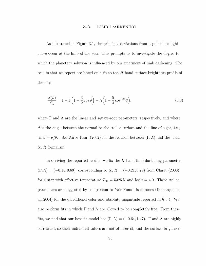
3.5. Limb Darkening

As illustrated in Figure 3.1, the principal deviations from a point-lens light

curve occur at the limb of the star. This prompts us to investigate the degree to

which the planetary solution is influenced by our treatment of limb darkening. The

results that we report are based on a fit to the H-band surface brightness profile of

the form

S(ϑ)

Sλ

= 1 − Γ(

1 − 3

2cos ϑ

)

− Λ(

1 − 5

4cos1/2 ϑ

)

, (3.8)

where Γ and Λ are the linear and square-root parameters, respectively, and where

ϑ is the angle between the normal to the stellar surface and the line of sight, i.e.,

sin ϑ = θ/θ∗. See An & Han (2002) for the relation between (Γ, Λ) and the usual

(c, d) formalism.

In deriving the reported results, we fix the H-band limb-darkening parameters

(Γ, Λ) = (−0.15, 0.69), corresponding to (c, d) = (−0.21, 0.79) from Claret (2000)

for a star with effective temperature Teff = 5325 K and log g = 4.0. These stellar

parameters are suggested by comparison to Yale-Yonsei isochrones (Demarque et

al. 2004) for the dereddened color and absolute magnitude reported in § 3.4. We

also perform fits in which Γ and Λ are allowed to be completely free. From these

fits, we find that our best-fit model has (Γ, Λ) = (−0.64, 1.47). Γ and Λ are highly

correlated, so their individual values are not of interest, and the surface-brightness

93

profiles generated by these two sets of (Γ, Λ) are qualitatively similar. In the present

context, however, the key point is that when we fix the limb-darkening parameters

at the Claret (2000) values, the contours in Figure 3.4 remain essentially identical

and the best fit values change by much less than 1σ.

Because of lower point-density and the aforementioned problems with the

I data over the peak, we only attempt a linear limb-darkening fit, i.e., we use

equation (3.8) with Λ ≡ 0, and we adopt Γ = 0.47 from Claret (2000).

3.6. Blended Light

In the crowded fields of the Galactic bulge, the photometered light of a

microlensing event rarely comes solely from the lensed source. Rather there is

typically additional light that is blended with the source but is not being lensed.

This light can arise from unrelated stars that happen to be projected close enough

to the line of sight to be blended with the source, or it can come from companions

to the source, companions to the lens, or the lens itself. This last possibility is most

interesting because, if the lens flux can be isolated and measured, it provides strong

constraints on the lens properties, and in this case would enable a complete solution

of the lens mass and distance, when combined with the measurement of θE (e.g.,

Bennett et al. 2007).

94

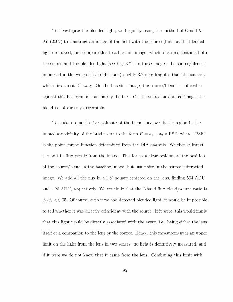
To investigate the blended light, we begin by using the method of Gould &

An (2002) to construct an image of the field with the source (but not the blended

light) removed, and compare this to a baseline image, which of course contains both

the source and the blended light (see Fig. 3.7). In these images, the source/blend is

immersed in the wings of a bright star (roughly 3.7 mag brighter than the source),

which lies about 2′′ away. On the baseline image, the source/blend is noticeable

against this background, but hardly distinct. On the source-subtracted image, the

blend is not directly discernible.

To make a quantitative estimate of the blend flux, we fit the region in the

immediate vicinity of the bright star to the form F = a1 + a2 × PSF, where “PSF”

is the point-spread-function determined from the DIA analysis. We then subtract

the best fit flux profile from the image. This leaves a clear residual at the position

of the source/blend in the baseline image, but just noise in the source-subtracted

image. We add all the flux in a 1.8′′ square centered on the lens, finding 564 ADU

and −28 ADU, respectively. We conclude that the I-band flux blend/source ratio is

fb/fs < 0.05. Of course, even if we had detected blended light, it would be impossible

to tell whether it was directly coincident with the source. If it were, this would imply

that this light would be directly associated with the event, i.e., being either the lens

itself or a companion to the lens or the source. Hence, this measurement is an upper

limit on the light from the lens in two senses: no light is definitively measured, and

if it were we do not know that it came from the lens. Combining this limit with

95

equation (3.6), and assuming the lens is a main-sequence star, it must then be less

massive than M < 0.75 M⊙, and so must have relative parallax πrel > 15 mas. This

implies a lens-source separation DS − DL > 1 kpc, which certainly does not exclude

bulge lenses. Indeed, if the lens were a K dwarf in the Galactic bulge, it would

saturate this limit.

3.7. Discussion

MOA-2007-BLG-400 is the first high-magnification microlensing event for which

the central caustic generated by a planetary companion to the lens is completely

enveloped by the source. As a comparison, the planetary caustic of OGLE-2005-

BLG-390 (Beaulieu et al. 2006) is smaller than its clump-giant source star in angular

size. When the planetary caustics is covered by the source, the finite-source effects

broaden the “classic” Gould & Loeb (1992) planetary perturbation features (Gaudi

& Gould 1997). By contrast, planet-induced deviations in MOA-2007-BLG-400 are

mostly obliterated, rather than being broadened, because the source crosses the

central caustic rather than the planetary caustic. We showed, nevertheless, that the

planetary character of the event can be inferred directly from the light-curve features

and that the standard microlensing planetary parameters (d, q) = (2.9, 2.5 × 10−3)

can be measured with good precision, up to the standard close/wide d ↔ d−1

degeneracy. We demonstrated that, in this case, the close/wide degeneracy is quite

96

severe, and the wide solution is only preferred by ∆χ2 = 0.2. This is unfortunate,

since the separations of the two solutions differ by a factor of ∼ 8.5. We argued that

the severity of this degeneracy was primarily related to the intrinsic parameters of

the planet, rather than being primarily a result of the large source size.

Although the mass ratio alone is of considerable interest for planet formation

theories, one would also like to be able to translate the standard microlensing

parameters to physical parameters, i.e., the planet mass mp = qM , and planet-star

projected separation r⊥ = dθEDL. Clearly this requires measuring the lens mass

M and distance DL. In this case, the pronounced finite source effects have already

permitted a measurement of the Einstein radius θE = 0.32 mas, which gives a relation

between the mass and lens-source relative parallax (eq. [3.6]). This essentially

yields a relation between the lens mass and distance, since the source distance is

close enough to the Galactic center that knowing DL is equivalent to knowing πrel.

Therefore, a complete solution could be determined by measuring either M or DL,

or some combination of the two.

One way to obtain an independent relation between the lens mass and distance

is to measure the microlens parallax, πE. There are two potential ways of measuring

πE. First, one can measure distortions in the light curve arising from the acceleration

of the Earth as it moves along its orbit. Unfortunately, this is out of the question

in this case because the event is so short that these distortions are immeasurably

small. Second, one can measure the effects of terrestrial parallax, which gives

97

rise to differences between the light curves simultaneously observed from two or

more observatories separated by a significant fraction of the diameter of the Earth.

Practically, measuring these differences requires a high-magnification event, which

would appear to make this event quite promising. Unfortunately, although we

obtained simultaneous observations from two observatories separated by several

hundred kilometers during the peak of the event, one of these datasets suffers from

large systematic errors and an unknown time zero point, rendering it unusable for

this purpose.

The only available alternative for breaking the degeneracy between the lens

mass and distance would be to measure the lens flux, either under the glare of the

source or, at a later date, to separately resolve it after it has moved away from the

line of sight to the source (Alcock et al. 2001a; Kozlowski et al. 2007). Panels (e)

and (f) of Figure 3.6 show the Bayesian estimates of the lens brightness in I-band

and H-band, respectively. If the lens flux is at least 2% of the source flux, then the

former kind of measurement could be obtained from a single epoch Hubble Space

Telescope observation, provided it were carried out in the reasonably near future. At

roughly 99% probability, the blended light would be either perfectly aligned with

the source (and so associated with the event) or well separated from it. HST images

can be photometrically aligned to the ground-based images using comparison stars

with an accuracy of better than 1%. Hence, photometry of the source+blend would

detect the blend, unless it were at least 4 mag fainter than the source. In principle,

98

the blend could be a companion to either the source or lens. Various arguments can

be used to constrain either of those scenarios. We do not explore those here, but see

Dong et al. (2009). If the lens is not detectable by current epoch HST observations

(or no HST observations are taken), then it will be detectable by ground-based AO

H-band observations in about 5 years. This is because the lens-source relative proper

motion is measured to be µrel = 8 mas yr−1, and the diffraction limit at H band on

a 10m telescope is roughly 35 mas. If the lens proves to be extremely faint, then a

wider separation (and hence a few years more time baseline) would be required.

In the absence of additional observational constraints, we must rely on a

Bayesian analysis to estimate the properties of the host star and planet, which

incorporates priors on the distribution of lens masses, distances, and velocities

(Dominik 2006; Dong et al. 2006). This is a standard procedure, which we only

briefly summarize here. We adopt a Han & Gould (1995) model for the Galactic

bar, a double-exponential disk with a scale height of 325 pc, and a scale length

of 3.5 kpc, as well as other Galactic model parameters as described in Bennett &

Rhie (2002). We incorporate constraints from our measurement of the lens angular

Einstein radius θE and the event timescale, as well as limits on the microlens parallax

and I-band magnitude of the lens. In practice, only the measurements of θE and tE

provide interesting constraints on these distributions. In addition, we include the

small penalty on the close solution, exp(−∆χ2/2), where the wide solution is favored

99

by ∆χ2 = 0.2. For the estimates of the planet semimajor axis, we assume circular

orbits and that the orbital phases and cos(inclinations) are randomly distributed.

The resulting probability densities for the physical properties of the host

star, as well as selected properties of the planet, are shown in Figure 3.6. The

Bayesian analysis suggests a host star of mass M = 0.30+0.19−0.12M⊙ at distance of

DL = 5.8+0.6−0.8 kpc. In other words, given the available constraints, the host is most

likely an M-dwarf, probably in the foreground Galactic bulge. Given that the

planet/star mass ratio is measured quite precisely, the probability distribution for

the planet mass is essentially just a rescaled version of the probability distribution

for the host star mass. We find mp = 0.83+0.49−0.31 MJup. The close/wide degeneracy

is apparent in the probability distribution for the semimajor axis a. We estimate

aclose = 0.72+0.38−0.16 AU for the close solution, and awide = 6.5+3.2

−1.2 AU for the wide

solution. The equilibrium temperatures for these orbits are Teq.,close = 103+28−26 K and

Teq.,wide = 34 ± 9 K for the close and wide solutions, respectively.

Thus our Bayesian analysis suggests that this system is mostly likely a

bulge mid-M-dwarf, with a Jovian-mass planetary companion. The semimajor

axis of the planetary companion is poorly constrained primarily because of the

close/wide degeneracy, but the implied equilibrium temperatures are cooler than the

condensation temperature of water. Specifically we find that Teq ∼< 173 K at 2σ

level. Alternatively, if we assume the snow line is given by asnow = 2.7 AU(M/M⊙),

we find for this system a snow line distance of ∼ 0.84 AU, essentially the same as

100

the inferred semimajor axis of the close solution. Thus this planet is quite likely to

be located close to or beyond the snow line of the system.

Although we cannot distinguish between the close and wide solutions for the

planet separation, theoretical prejudice in the context of the core-accretion scenario

would suggest that a gas-giant planet would be more likely to form just outside

the snow line, thus preferring the close solution. However, we have essentially no

observational constraints on the frequency and distribution of Jupiter-mass planets

at the separations implied by the wide solution (∼ 5.3 − 9.7 AU), for such low-mass

primaries. Unfortunately, the prospects for empirically resolving the close/wide

degeneracy in the future are poor. The only possible method of doing this would

be to measure the radial velocity signature of the planet. Given the faintness of

the host star (see §3.6 and Fig. 3.6), this will likely be impossible with current or

near-future technology.

The mere existence of a gas-giant planet orbiting a mid-M-dwarf is largely

unexpected in the core-accretion scenario, as formation of such planets is thought

to be inhibited in such low-mass primaries (Laughlin et al. 2004). Observationally,

however, although the frequency of Jovian companions to M-dwarfs with a ∼< 3 AU

does appear to be smaller than the corresponding frequency of such companions

to FGK dwarfs (Endl et al. 2006; Johnson et al. 2007b; Cumming et al. 2008),

several Jovian-mass companions to M dwarfs are known (see Dong et al. 2009 for

a discussion), so this system would not be unprecedented. Furthermore, it must

101

be kept in mind that the estimates of stellar (and so planet) mass depend on the

validity of the priors, and even in this context have considerable uncertainties.

Most of the ambiguities in the interpretation of this event would be removed

with a measurement of the host star mass and distance, which could be obtained by

combining our measurement of θE with a measurement of the lens light as outlined

above. The Bayesian analysis informs the likelihood of success of such an endeavor.

This analysis suggests that, if the host is a main-sequence star, its magnitude will

be IL = 23.9+0.8−1.0 and HL = 21.4+0.7

−1.0, which corresponds to 0.6% and 1.7% of the

source flux, respectively. If initial efforts to detect the lens fail, more aggressive

observations would certainly be warranted: microlensing is the most sensitive

method for detecting planets around very low-mass stars simply because it is the

only method that does not rely on light from the host (or the planet itself) to detect

the planet. And given equation (3.6), even an M dwarf at the very bottom of the

main sequence M = 0.08 M⊙, would lie at DL = 3.5 kpc and so would be H ∼ 24.

102

HJD - 2454354.0

Fig. 3.1.— Top: Lightcurve of MOA-2007-BLG-400 with data from µFUN CTIO(Chile) simultaneously taken in H (cyan), I (DIA, black). Models are shown for apoint lens (blue) and planet-star system (red). There are 5 50-second H exposures foreach 300-second I (or V – not shown) exposure in 6 minutes cycles. Some I-band dataat the peak suffer from saturation, and those points are therefore removed from theanalysis (see text). Middle: Residuals for best-fit point-lens model and its differencewith the planetary model. Note that in the top panel, the H data are shown asobserved, while the I data are aligned. Normally, such alignment is straightforwardbecause microlensing of point sources is achromatic. However, here there is significantchromaticity due to different limb-darkening. The I-band points in the top panel areactually the residuals to the I-band limb-darkened model (middle panel), added tothe H-band model curve (top panel). Bottom: Residuals from a point-lens modelwith the same parameters as the planetary model, which can be directly compared tothe “magnification map” in Fig. 3.3. These “didactic residuals” are naturally morepronounced than those from the best-fit point lens.

103

Fig. 3.2.— Comparisons of residuals to the best-fit point-lens models between twophotometric reductions of µFUN H-band data, using the DIA packages developedby Wozniak (2000) (top) and Bond et al. (2001) (bottom). The red curve in eachpanel represents the difference of the best-fit planetary and point-lens models for thatpanel’s reduction. Both reductions agree on the main planetary features, but eachpackage introduces its own systematics. For example, the systematic deviations fromthe planetary model at HJD ∼ 2454354.57 shown in the top panel are not supportedby the reductions of the Bond’s package. During 2454354.46 < HJD < 2454354.51,most images have low transparency (∼< 50%), which causes relatively large scatter inBond’s DIA reductions. In comparison, the reduction by Wozniak’s DIA has smallerscatter during this period. However, the data exhibit some low-level systematics,which are not supported by the other reduction.

104

Fig. 3.3.— Magnification differences between of best-fit planetary model [(q, d) =(0.0025, 2.9) and (q, d) = (0.0026, 0.34) being nearly identical] and single-lens models,in units of the measured source size, ρ = 0.0033 Einstein radii. Contours show 1%, 2%,3%, and 4%, deviations in the positive (brown) and negative (blue) directions. Toppanel: Single-lens geometry (t0, u0, tE) is taken to be the same as in the planetarymodel, with no finite source effects. Caustic (contour of infinite magnification) isshown in white. The deviations are very pronounced. Bottom Panel: Same as toppanel, but including finite-source effects, which now explain the main features of thelight curve. The trajectory begins with a negative deviation, then hits a narrow“brown ridge” causing the spike seen in the bottom panel of Fig. 3.1, as the edgeof the source first hits the caustic. Then there are essentially no deviations (white)while the source covers the caustic. The caustic exit induces a narrow “blue ridge”corresponding to the negative-deviation spike seen in Fig 3.1. Finally, the source runsalong the long “brown ridge” corresponding to the prolonged post-peak mild excessseen in Fig 3.1.

105

Fig. 3.4.— Contours of ∆χ2 = 1, 4, 9 relative to the minimum as a function of planet-star mass ratio q and projected planet-star separation d (top), as well as “short causticdiameter” (see Fig. 3.3) w (bottom). w (in units of θE) is a function of q and d (seetext). The solution shown here corresponds to q = (2.5+0.5

−0.3)×10−3 and d = 2.9±0.2 (ord = 0.34+0.03

−0.02). These values of d correspond to physical separations and equilibriumtemperatures of ∼ 5.3 − 9.7 AU, ∼ 34 K and ∼ 0.6 − 1.1 AU, ∼ 103 K for the closeand wide solutions, respectively.

106

(V−I) [instrumental]

I [in

stru

men

tal]

−.6 −.4 −.2 0 .2

22

20

18

16

Fig. 3.5.— Instrumental color-magnitude diagram of field containing MOA-2007-BLG-400. The color and magnitude of the source (black filled circle) are derived fromthe fit to the light curve, which also yields an upper limit for the I-band blendedflux (green triangle). The large error bar on the latter point indicates a completelack of information about its V -band flux. The clump centroid is indicated in redsquare. From the source-clump offset, we estimate [I, (V − I)]0,s = (17.57, 0.81),implying it has angular radius θ∗ = 1.05 µas. Assuming the source lies at 8 kpc, ithas [MI , (V − I)]0,s = (3.07, 0.81), making it a subgiant. The lack of blended lightallows us to place an upper limit on the lens flux, which implies that it has massM < 0.75 M⊙. See text.

107

Fig. 3.6.— Bayesian relative probability densities for the physical properties of theplanet MOA-2007-BLG-400Lb and its host star. (a) Mass of the host star. (b) Planetsemimajor axis. (c) Distance to the planet/star system. (d) Equilibrium temperatureof the planet. (e) I-band magnitude of the host star. (f) H-band magnitude of thehost star. In panel (a), we also show the probability density for the planet mass, whichis essentially a rescaling of that of the host star, because the mass ratio is measuredso precisely q = (2.5+0.5

−0.3) × 10−3. In all panels, the solid vertical lines show themedians, and the 68.3% and 95.4% confidence intervals are enclosed in the dark andlight shaded regions, respectively. In panel (b) and (d), the probability distributionsfor wide and close degenerate solutions are computed separately, and then the closesolution is weighted by exp(−∆χ2/2), where ∆χ2 = 0.2 is the difference betweenthem. These distributions are derived assuming priors obtained from standard modelsof the mass, velocity, and density distributions of stars in the Galactic bulge and disk,and include constraints from the measurements of lens angular Einstein radius θE andthe timescale of the event tE, as well as limits on the I-band magnitude of the lens.In practice, only the measurements of θE and tE provide interesting constraints onthese distributions.

108

B) BASELINE A) PEAKPEAK

D) BASELINE - SOURCE C) PEAK - BASELINE

Fig. 3.7.— Constraining the blended flux from CTIO I-band images. A good-seeingbaseline image B (upper right) is subtracted from an image taken at magnification245 (A, upper left), and the resulting image C is shown in the bottom-left panel.The white circles on images A and C indicate the source positions. Then C is scaledby 1/244 in flux and subtracted from image B to generate image D, which has thesource contribution removed from the baseline image. As described in the text, we fitPSF to the stars close to the source, and subtract them from images B and D. Aftersubtraction, the flux sums in a 1.8” square (shown as black boxes on right two panels)are 564 ADU and -28 ADU, respectively. Non-detection of the blend constrains theblend-source flux ratio to be less than 5%.

109

Model1 t0 − tref2 u0 tE d q α3 ρ

day day deg

Close 0.08107 0.00025 14.41 0.34 0.0026 227.06 0.00326

Wide 0.08106 0.00027 14.33 2.87 0.0025 226.99 0.00329

1The wide solution is preferred over best-fit single-lens model by ∆χ2 =

1070.04 and the close solution by ∆χ2 = 1069.84

2tref = HJD 2454354.5 (Sep 11, 2007, 00:00 UT).

3The geometry of the source trajectory is visualized in Figure 3.3, in

which the planet is to the right of the lens star. t0, u0, and α are defined

with respect to the “center of magnification”, which is the center of mass

of the star/planet system for the close model and q/(1 + q)/d away from

the position of the lens star toward the direction of the planet for the wide

model.

Table 3.1. MOA-2007-BLG-400 Best-fit Planetary Models

110

Chapter 4

OGLE-2005-BLG-071Lb, the Most Massive

M-Dwarf Planetary Companion?

4.1. Introduction

Microlensing provides a powerful method to detect extrasolar planets. Although

only six microlens planets have been found to date (Bond et al. 2004; Udalski et al.

2005; Beaulieu et al. 2006; Gould et al. 2006; Gaudi et al. 2008; Dong et al. 2009),

these include two major discoveries. First, two of the planets are “cold Neptunes”,

a high discovery rate in this previously inaccessible region of parameter space,

suggesting this new class of extrasolar planets is common (Gould et al. 2006; Kubas

et al. 2008). Second, the discovery of the first Jupiter/Saturn analog via a very

high-magnification event with substantial sensitivity to multiple planets indicates

that solar system analogs may be prevalent among planetary systems (Gaudi et al.

2008). Recent improvements in search techniques and future major upgrades should

increase the discovery rate of microlensing planets substantially (Gaudi 2008).

111

Routine analysis of planetary microlensing light curves yields the planet/star

mass ratio q and the planet-star projected separation d (in units of the angular

Einstein radius). However, because the lens-star mass M cannot be simply extracted

from the light curve, the planet mass Mp = qM remains, in general, equally

uncertain.

The problem of constraining the lens mass M is an old one. When microlensing

experiments were initiated in the early 1990s, it was generally assumed that

individual mass measurements would be impossible and that only statistical

estimates of the lens mass scale could be recovered. However, Gould (1992) pointed

out that the mass and lens-source relative parallax, πrel ≡ πl − πs, are simply related

to two observable parameters, the angular Einstein radius, θE, and the Einstein

radius projected onto the plane of the observer, rE,

M =θE

κπE

, πrel = θEπE. (4.1)

Here, πE = AU/rE is the “microlens parallax” and κ ≡ 4G/(c2 AU) ∼ 8.1 mas/M⊙.

See Gould (2000b) for an illustrated derivation of these relations.

In principle, θE can be measured by comparing some structure in the light curve

to a “standard angular ruler” on the sky. The best example is light-curve distortions

due to the finite angular radius of the source θ∗ (Gould 1994a), which usually can be

estimated very well from its color and apparent magnitude (Yoo et al. 2004a). While

112

such finite-source effects are rare for microlensing events considered as a whole, they

are quite common for planetary events. The reason is simply that the planetary

distortions of the light curve are typically of similar or smaller scale than θ∗. In fact,

all six planetary events discovered to date show such effects. Combining θE with the

(routinely measurable) Einstein radius crossing time tE yields the relative proper

motion µ in the geocentric frame,

µgeo =θE

tE, (4.2)

From equation (4.1), measurement of θE by itself fixes the product Mπrel = θ2E/κ.

Using priors on the distribution of lens-source relative parallaxes, one can then make

a statistical estimate of the lens mass M and so the planet mass Mp.

To do better, one must develop an additional constraint. This could be

measurement of the microlens parallax πE, but this is typically possible only for long

events. Another possibility is direct detection of the lens, either under the “glare” of

the source during and immediately after the event, or displaced from the source well

after the event is over. Bennett et al. (2006) used the latter technique to constrain the

mass of the first microlensing planet, OGLE-2003-BLG-235/MOA-2003-BLG-53Lb.

They obtained Hubble Space Telescope (HST) Advanced Camera for Surveys (ACS)

images in B, V , and I at an epoch ∆t = 1.78 years after the event. They found

astrometric offsets of the (still overlapping) lens and source light among these images

of up to 0.7 mas. Knowing the lens-source angular separation ∆θ = µ∆t from the

113

already determined values of θE and tE, they were able to use these centroid offsets to

fix the color and magnitude of the lens and so (assuming that it was a main-sequence

star) its mass.

While the planet mass is usually considered to be the most important

parameter that is not routinely derivable from the light curve, the same degeneracy

impacts two other quantities as well, the distance and the transverse velocity of

the lens. Knowledge of these quantities could help constrain the nature of the

lens, that is, whether it belongs to bulge, the foreground disk, or possibly the

thick disk or even the stellar halo. Since microlensing is the only method currently

capable of detecting planets in populations well beyond the solar neighborhood,

extracting such information would be quite useful. Because the mass, distance,

and transverse velocity are all affected by a common degeneracy, constraints on

one quantity are simultaneously constraints on the others. As mentioned above,

simultaneous measurements of θE and πE directly yield the mass. However,

clearly from equation (4.1) they also yield the distance, and hence (from eq. [4.2])

also the transverse velocity. Here, we assemble all available data to constrain

the mass, distance and transverse velocity of the second microlensing planet,

OGLE-2005-BLG-071Lb, whose discovery we previously reported (Udalski et al.

2005, hereafter Paper I).

114

4.2. Overview of Data and Types of Constraints

The light curve consists of 1398 data points from 9 ground-based observatories

(see Fig. 2.1), plus two epochs of HST ACS data in the F814W (I) and F555W

(V ) filters. The primary ground-based addition relative to Paper I is late-time data

from OGLE, which continued to monitor the event down to baseline until HJD

= 2453790.9.

These data potentially provide constraints on several parameters in addition to

those reported in Paper I. First, the light curve shows a clear asymmetry between

the rising and falling parts of the light curve, which is a natural result of microlens

parallax due to the Earth’s accelerated motion around the Sun (see the best-fit

model without parallax effects plotted in dotted line in Fig. 2.1). However, it

is important to keep in mind that such distortions are equally well produced by

“xallarap” due to accelerated motion of the source around a companion. Poindexter

et al. (2005) showed that it can be difficult to distinguish between the two when, as

in the present case, the effect is detected at ∆χ2 <∼ 100.

Second, the two pronounced peaks of the light curve, which are due to “cusp

approaches” (see the bottom inset of Fig. 2.1), are relatively sharp and have good

coverage. These peaks would tend to be “rounded out” by finite-source effects, so

in principle it may be possible to measure ρ (i.e., θ∗ in the units of θE) from these

distortions.

115

Third, the orbital motion of the planet can give rise to two effects: rotation

of the caustic about the center of the mass and distortion of the caustic due to

expansion/contraction of the planet-star axis. The first changes the orientation of

the caustic structure as the event evolves while the second changes its shape. These

effects are expected to be quite subtle because the orbital period is expected to be

of an order of 10 years while the source probes the caustic structure for only about 4

days. Nevertheless, they can be very important for the interpretation of the event.

Finally, the HST data cover two epochs, one at 23 May 2005 (indicated by the

arrow in Fig. 2.1) when the magnification was about A = 2 and the other at 21 Feb

2006 when the event was very nearly at baseline, A ∼ 1. These data could potentially

yield four types of information. First, they can effectively determine whether the

blended light is “associated” with the event or not. The blended light is composed

of sources in the same photometric aperture as the magnified source, but that do

not become magnified during the event. If this light is due to the lens, a companion

to the lens, or a companion to the source, it should fall well within the ACS point

spread function (PSF) of the source. On the other hand, if it is due to a random

interloper along the line of sight, then it should be separately resolved by the ACS

or at least give rise to a distorted PSF. Second, the HST data can greatly improve

the estimate of the color of the blended light. The original model determined the

source fluxes in both OGLE V and I very well, and of course the baseline fluxes

are also quite well determined. So it would seem that the blended fluxes, which are

116

the differences between these two, would also be well determined. This proves to be

the case in the I band. However, while the source flux is derivable solely from flux

differences over the light curve (and so is well determined from OGLE difference

image analysis – DIA – Wozniak 2000), the baseline flux depends critically on the

zero point of PSF-fitting photometry, whose accuracy is fundamentally limited in

very crowded bulge fields. The small zero-point errors turn out to have no practical

impact for the relatively bright I background light, but are important for the V

band. Third, one might hope to measure a centroid shift between the two colors in

the manner of Bennett et al. (2006). Last, one can derive the source proper motion

µs from HST data (at least relative to the mean motion of bulge stars). This is

important, because the event itself yields the source-lens relative proper motion,

µgeo. Hence, precise determination of µl requires knowledge of two proper-motion

differences, first the heliocentric proper motion

µhel = µl − µs, (4.3)

and second, the offset between the heliocentric and geocentric proper motions

µhel − µgeo =v⊕πrel

AU. (4.4)

Here, v⊕ is the velocity of the Earth relative to the Sun at the time of peak

magnification t0. Note that, if the lens-source relative parallax πrel is known, even

117

approximately, then the latter difference can be determined quite well, since its total

magnitude is just 0.6 mas yr−1(πrel/0.17 mas).

4.3. Constraining the Physical Properties of the Lens

and its Planetary Companion

In principle, all the effects summarized in § 4.2 could interact with each

other and with the parameters previously determined, leading potentially to a very

complex analysis. In fact, we will show that most effects can be treated as isolated

from one another, which greatly facilitates the exposition. In the following sections,

we will discuss the higher order microlens effects in the order of their impact on

the ground-based light curve, starting with the strongest, that is, parallax effects

(§ 4.3.1), followed by planetary orbital motion (§ 4.3.2) and finally the weakest,

finite-source effects (§ 4.3.3). To study these effects, we implement Markov chain

Monte Carlo (MCMC) with an adaptive step-size Gaussian sampler (Doran &

Mueller 2003) to perform the model fitting and obtain the uncertainties of the

parameters. The HST astrometry is consistent with no (V − I) color-dependent

centroid shift in the first epoch, while such a shift is seen in the second epoch

observations (§ 4.3.4). In addition, the PSF of the source shows no sign of broadening

due to the blend, suggesting that the blend is associated with the event (§ 4.3.5).

Therefore, the HST observations provide good evidence that the blend is likely due

118

to the lens. In § 4.3.4, it is shown, under such an assumption, how the astrometry

can be used in conjunction with finite-source and microlens parallax measurements

to constrain the angular Einstein radius and proper motion (§ 4.3.4). In § 4.3.5,

we discuss using HST photometric constraints in the form of χ2 penalties to the

MCMC runs to extract the color and brightness of the blend. The results of these

runs, which include all higher order effects of the ground-based light curve and the

HST photometric constraints, are summarized as “MCMC A” in Table 4.1 and

4.2. Subsequently in § 4.3.6, by making the assumption that the blended light seen

by HST is due to the lens, we combine all constraints discussed above to obtain

physical parameters of the lens star and its planet. The corresponding best-fit model

parameters are reported as “MCMC B” in Table 4.3 and 4.4. The results for the

physical parameters from these runs are given in Table 4.5. Finally we discuss some

caveats in the analysis in § 4.3.7 and § 4.3.8.

4.3.1. Microlens Parallax Effects

A point-source static binary-lens model has 6 “geometric-model” parameters:

three “single-lens” parameters (t0, u0, tE), where we define the time of “peak”

magnification (actually lens-source closest approach) t0 and the impact parameter u0

with respect to the center of mass of the planet-star systems; and three “binary-lens”

parameters (q, d, α), where α is the angle between the star-planet axis and the

trajectory of the source relative to the lens. In addition, flux parameters are included

119

to account for light coming from the source star (Fs) and the blend (Fb) for each

dataset. In this paper, we extend the fitting by including microlens parallax, orbital

motion and finite-source effects. Paper I reported that, within the context of the

point-source static binary-lens models, the best-fit wide-binary (d > 1) solution is

preferred by ∆χ2 = 22 over the close-binary (d < 1) solution. Remarkably, when we

take account of parallax, finite-source and orbital effects, this advantage is no longer

as significant. We discuss the wide/close degeneracy with more detail in § 4.3.6.

The microlens parallax effects are parametrized by πE,E and πE,N, following the

geocentric parallax formalism by An et al. (2002) and Gould (2004). To properly

model the parallax effects, we characterize the “constant acceleration degeneracy”

(Smith et al. 2003) by probing models with u0 → −u0 and α → −α. We find that

all other parameters remain essentially unchanged under this form of degeneracy.

In the following sections, if not otherwise specified, parameters from models with

positive u0 are adopted.

As shown in Figure 4.2, microlens parallax is firmly detected in this event at

> 8σ level. Not surprisingly, the error ellipse of πE is elongated toward πE,⊥, i.e., the

direction perpendicular to the position of the Sun at the peak of event, projected

onto the plane of the sky (Gould et al. 1994; Poindexter et al. 2005). As a result,

πE,E is much better determined than πE,N,

πE,E = −0.26 ± 0.05, πE,N = −0.30+0.24−0.28 (wide), (4.5)

120

πE,E = −0.27 ± 0.05, πE,N = −0.36+0.24−0.27 (close). (4.6)

Xallarap (light-curve distortion from reflex motion of the source due to a binary

companion) could provide an alternate explanation of the detected parallax signals.

In § 4.3.8, we find that the best-fit xallarap parameters are consistent with those

derived from the Earth’s orbit, a result that favors the parallax interpretation.

4.3.2. Fitting Planetary Orbital Motion

To model orbital motion, we adopt the simplest possible model, with uniform

expansion rate b in binary separation b and uniform binary rotation rate ω. Because

orbital effects are operative only for about 4 days, while the orbital period is of

order 10 years, this is certainly adequate. Interestingly, the orbital motion is more

strongly detected for the close solutions (at >∼ 5.5σ level) than the wide solutions (at

∼ 3σ level), and as a result, it significantly lessens the previous preference of the

wide solution that was found before orbital motion was taken into account. Further

discussions on planetary orbital motion are given in § 4.3.6.

121

4.3.3. Finite-source effects and Other Constraints on

θE

Color-Magnitude Diagram

We follow the standard procedure to derive dereddened source color and

magnitude from the color-magnitude diagram (CMD) of the observed field.

Figure 4.3 shows the calibrated OGLE CMD (black), with the baseline source

being displayed as a green point. The V − I color of the source can be determined

in a model-independent way from linear regression of the I-band and V -band

observations. The I-band magnitude of the source is also precisely determined from

the microlens model, and it is hardly affected by any higher order effects. The center

of red clump (red) is at (V − I, I)clump = (1.89, 15.67). The Galactic coordinates of

the source are at (l, b) = (355.58,−3.79). Because the Galactic bulge is a bar-like

structure that is inclined relative to the plane of the sky, the red clump density

at this sky position peaks behind the Galactic center by 0.15 mag (Nishiyama

2005). Hence, we derive (V − I, I)0,clump = (1.00, 14.47), by adopting a Galactic

distance R0 = 8 kpc. We thereby obtain the selective and total extinction toward

the source [E(V − I), AI ] = (0.89, 1.20) and thus RV I = AV /E(V − I) = 2.35. The

dereddened color and magnitude of the source is ((V − I), I)s,0 = (0.45, 18.31). From

its dereddened color (V − I)0 = 0.45, as well as its absolute magnitude (assuming it

is in the bulge) MI ∼ 3.65, we conclude that the source is a main-sequence turnoff

122

star. Following the method of Yoo et al. (2004a), we transform (V − I)0 = 0.45 to

(V −K)0 = 0.93 (Bessell & Brett 1988), and based on the empirical relation between

the color and surface brightness for subgiant and main-sequence stars (Kervella et

al. 2004), we obtain the angular size of the source

θ∗ = 0.52 × 100.2(19.51−Is) ± 0.05 µas, (4.7)

where Is is the apparent magnitude of the source in the I band. Other features on

the CMD shown in Figure 4.3 are further discussed in § 4.3.5.

Photometric Systematics of the Auckland Data set

The Auckland data set’s excellent coverage over the two peaks makes it

particularly useful for probing the finite-source effects. Unlike the more drastic

“caustics crossings” that occur in some events, the finite-source effects during “cusp

approaches” are relatively subtle. Hence one must ensure that the photometry is not

affected by systematics at the few percent level when determining ρ = θ∗/θE. The

Auckland photometry potentially suffers from two major systematic effects.

First, the photometry of constant stars reduced by µFUN’s DoPHOT pipeline

are found to show sudden “jumps” of up to ∼ 10% when the field crossed the

meridian each night. The signs and amplitudes of the “jumps” depend on the

stars’ positions on the CCD. The Auckland telescope was on a German equatorial

mount, and hence the camera underwent a meridian flip. Due to scattered light,

123

the flat-fielded images were not uniform in illumination for point sources, an effect

that can be corrected by making “superflats” with photometry of constant stars

(Manfroid 1995). We have constructed such “superflats” for each night of Auckland

observations using 71 bright isolated comparison stars across the frame. The

DoPHOT instrumental magnitude mi,j for star i on frame j is modeled by the

following equation:

mi,j = m0,i − f(xi,j, yi,j) − Zj − fwhmi,j × si (4.8)

where m0,i is the corrected magnitude for star i, f(x, y) is a biquartic illumination

correction as a function of the (x, y) position on the CCD frame with 14 parameters,

Zj is a zero-point parameter associated with each frame (but with Z1 set to be zero),

and si is a linear correlation coefficient for the seeing fwhmi,j. A least-squares fit

that recursively rejects 4-σ outliers is performed to minimize χ2. The best-fit f(x, y)

is dominated by the linear terms and has small quadratic terms, while its cubic and

quartic terms are negligible. The resulting reduced χ2 is close to unity, and the

“jumps” for all stars are effectively eliminated. We apply the biquartic corrections

to the images and then reduce the corrected images using the DIA pipeline. The

resulting DIA photometry of the microlens target is essentially identical (at the

∼ 1% level) to that from the DIA reductions of the original Auckland images.

As we now show, this is because DIA photometry automatically removes any

artifacts produced by the first- and second-order illumination distortions if the

124

sources are basically uniformly distributed across the frame. For the first-order

effect, a meridian flip about the target (which is very close to center of the frame)

will induce a change in the flux from the source, but it will also induce a change in

the mean flux from all other stars in the frame, which for a linear correction will

be the same as the change in position of the “center of light” of the frame light.

If the frame sources are uniformly distributed over the frame, the “center of light”

will be the center of the frame, which is the same position as the source, therefore

introducing no effects. The second-order transformation is even under a rotation of

180 degrees, whereas a meridian flip is odd under this transformation. Hence the flip

has no effects at second order.

Second, the Auckland observations were unfiltered. The amount of atmospheric

extinction differs for stars with different colors. As shown in Figure 4.3, the source is

much bluer than most of the bright stars in the field, which dominate the reference

image. So the amount of extinction for the source is different from the average

extinction over the whole frame. This difference varies as the airmass changes over

time during the observations. Coincidentally, the times of the two peaks were both

near maximum airmass when the “differential extinction” effect is expected to be the

most severe. To investigate this effect, we match the isolated stars in the Auckland

frame with CTIO I and V photometry. We identify 33 bright, reasonably isolated

stars with |(V − I) − (V − I)s| < 0.25. We obtain a “light curve” for each of these

stars, using exactly the same DIA procedure as for the source. We measure the

125

mean magnitude of each of the 33 light curves and subtract this value from each of

the 508 points on each light curve, thereby obtaining residuals that are presumably

due primarily to airmass variation. For each of the 508 epochs, we then take the

mean of all of these residuals. We recursively remove outliers until all the remaining

points are within 3σ of the mean, as defined by the scatter of the remaining points.

Typically, 1 or 2 of the 33 points are removed as outliers. The deviations are well

fitted by a straight line,

dMag

dZ= 0.0347 ± 0.0016 (4.9)

where Z is airmass. The sense of the effect is that stars with the color of the

microlensed source are systematically fainter at high airmass, as expected. (We also

tried fitting the data to a parabola rather than a line, but the additional [quadratic]

parameter was detected at substantially below 1σ.) Finally, we apply these

“differential extinction” corrections to the “superflat”-adjusted DIA photometry to

remove both photometric systematics.

In general, the finite-source effects depend on the limb-darkening profile of the

source star in the observed passbands. We find below that in this case, the impact

proves to be extremely weak. Nevertheless, using the matched Auckland and CTIO

stars, we study the difference between Auckland magnitudes and I-band magnitude

as a function of the V − I color. We find the Auckland clear filter is close to the R

band.

126

Blending in Palomar and MDM Data

Palomar data cover only about 80 minutes, but these include the cresting of

the second peak, from which we derive essentially all information about finite-source

effects. The Palomar data are sensitive to these effects through their curvature.

The curvature derived from the raw data can be arbitrarily augmented in the fit

(and therefore the finite-source effects arbitrarily suppressed) by increasing the

blending. In general, the blending at any observatory is constrained by observations

at substantially different magnifications, typically on different nights. However, no

such constraints are available for Palomar, since observations were carried out on

only one night.

We therefore set the Palomar blending fb = 0.2 fs, that is, similar to the OGLE

blending. That is, we assume that the observed flux variation of 9%, over the Palomar

night, actually reflects a magnification variation of 9%/[1 − fb/Afs] = 9% + 0.026%,

where A ∼ 70 is the approximate magnification on that night. If our estimate of the

blending were in error by of order unity (i.e. either fb = 0 or fb = 0.4 fs), then the

implied error in the magnification difference would be 0.026%, which is more than an

order of magnitude below the measurement errors. Hence, the assumption of fixed

blending does not introduce “spurious information” into the fit even at the 1 σ level.

MDM data cover the second peak for only ∼ 18 minutes. For consistency, we treat

127

its blending in the same way as Palomar, although the practical impact of this data

set is an order of magnitude smaller.

Modeling the Finite-Source Effects

After careful tests that are described immediately below, we determined that

all finite-source calculations can be carried out to an accuracy of 10−4 using the

hexadecapole approximation of Gould (2008) (see also Pejcha & Heyrovsky 2008).

This sped up calculations by several orders of magnitude. We began by conducting

MCMC simulations using the “loop linking” finite-source code described in Appendix

A of Dong et al. (2006). From these simulations, we found the 4.5 σ upper bound

on the finite-source parameter ρ(4.5 σ) = 0.001. We then examined the differences

between loop-linking (set at ultra-high precision) and hexadecapole for light curves at

this extreme limit and found a maximum difference of 10−4. Based on Claret (2000),

we adopt linear limb-darkening coefficients ΓI = 0.35 for the I-band observations and

ΓR = 0.43 for the observations performed in the R-band and the clear filters, where

the local surface brightness is given by S(θ) ∝ 1 − Γ[1 − 1.5(1 − θ2/θ2∗)

1/2]. Ten

additional MCMC runs are performed with ΓI and ΓR that differ from the above

values by 0.1 or 0.2. They result in essentially the same probability distributions of

ρ. Therefore, the choice of limb-darkening parameters has no effect on the results.

The source size is found to be ρ = 3.9+1.8−2.7 for the wide solution and ρ = 3.1+1.7

−2.5 for the

close solution. Solutions with ρ > 0.0009 are ruled out at more than 3σ. The angular

128

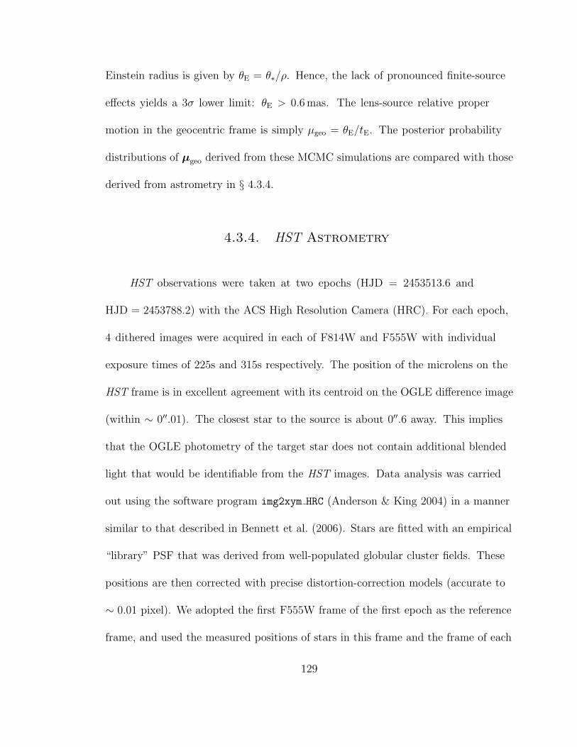
Einstein radius is given by θE = θ∗/ρ. Hence, the lack of pronounced finite-source

effects yields a 3σ lower limit: θE > 0.6 mas. The lens-source relative proper

motion in the geocentric frame is simply µgeo = θE/tE. The posterior probability

distributions of µgeo derived from these MCMC simulations are compared with those

derived from astrometry in § 4.3.4.

4.3.4. HST Astrometry

HST observations were taken at two epochs (HJD = 2453513.6 and

HJD = 2453788.2) with the ACS High Resolution Camera (HRC). For each epoch,

4 dithered images were acquired in each of F814W and F555W with individual

exposure times of 225s and 315s respectively. The position of the microlens on the

HST frame is in excellent agreement with its centroid on the OGLE difference image

(within ∼ 0′′.01). The closest star to the source is about 0′′.6 away. This implies

that the OGLE photometry of the target star does not contain additional blended

light that would be identifiable from the HST images. Data analysis was carried

out using the software program img2xym HRC (Anderson & King 2004) in a manner

similar to that described in Bennett et al. (2006). Stars are fitted with an empirical

“library” PSF that was derived from well-populated globular cluster fields. These

positions are then corrected with precise distortion-correction models (accurate to

∼ 0.01 pixel). We adopted the first F555W frame of the first epoch as the reference

frame, and used the measured positions of stars in this frame and the frame of each

129

exposure to define a linear transformation between the exposure frame and the

reference frame. This allowed us to transform the position of the target star in each

exposure into the reference frame, so that we see how the target star had moved

relative to the other stars. The centroid positions of the target star in each filter

and epoch are shown in Figure 4.4. For convenience, in this figure, the positions are

displayed relative to the average of the centroid positions. The error bars are derived

from the internal scatter of the four dithered images. The probability is P = 38%

of measuring the observed separation (or larger) between F814W and F555W under

the assumption that the true offset is zero. The fact that the blended light is aligned

with the source argues that it is associated with the event (either it is the lens itself

or a companion to the lens or the source). We give a more quantitative statement

of this constraint in § 4.3.5. For the present we simply note that the P = 38%

probability is compatible with the picture that the blend is due to the lens since the

first epoch was only about half of the Einstein-radius crossing time after t0, implying

that the lens-source separation induces only a very small centroid offset, well below

the HST detection limit. For the second epoch, the centroid offset is,

∆rF814W−F555W,East = −0.52 ± 0.20 mas,

∆rF814W−F555W,North = 0.22 ± 0.20 mas. (4.10)

130

We also calculate the error in the centroid offsets from the scatter in such

offsets among all comparison stars with F555W magnitudes within 0.5 mag of the

target and find that it is consistent with the internally-based error quoted above.

At the peak of the event, the angular separation between the lens and the

source was negligible, since u0 ≪ 1. We therefore fix the angular positions of the

lens and source at a common θ0. From the CMD (Fig. 4.3), most of the stars in the

HST field are from the bulge. So we set a reference frame that is fixed with respect

to the bulge field at distance Ds. The source and lens positions at time t are then,

θs(t) = θ0 + µs(t − t0),

θl(t) = θ0 + µl(t − t0) + πrel[s(t) − s(t0)], (4.11)

where s(t) is the Earth-to-Sun vector defined by Gould (2004). Then by applying

equations (4.3) and (4.4), the angular separation between the lens and source is,

θrel(t) = θl(t) − θs(t) = µgeo(t − t0) + πrel∆s(t) (4.12)

where ∆s(t) is given by eq. (5) in Gould (2004).

The centroid of the source images θ′s is displaced from the source position by

(Walker 1995),

131

∆θs(t) = θ′

s(t) − θs(t) =

−θrel(t)

[θrel(t)/θE]2 + 2(4.13)

Therefore, one can obtain the centroid position of the lens and the source at

time t,

θc(t) = [1 − fl(t)][θs(t) + ∆θs(t)] + fl(t)θl(t)

= θ0 + µs(t − t0) + θrel(t)[fl(t) +1 − fl(t)

[θrel(t)/θE]2 + 2] (4.14)

where fl(t) is the fraction of the total flux due to the lens.

The centroid offset between the two passbands, F814W and F555W, is related

to the properties of the system by,

∆θc(t)F814W−F555W = [f(t)l,F814W−f(t)l,F555W]×[1− 1

[θrel(t)/θE]2 + 2]θrel(t).(4.15)

The difference of the blend’s fractional flux between F814W and F555W is obtained

from “MCMC A” described in § 4.3.5. Consequently, under the assumption that the

blend is the lens, we can use the measurement of the second-epoch HST centroid

offset to estimate the relative proper motion from equation (4.15) for a given πrel.

For purposes of illustration, we temporarily adopt πrel = 0.2 when calculating the

probability distribution of µgeo (black contours in the upper panels of Fig. 4.5). The

132

centroid shift generally favors faster relative proper motion than that derived from

the source size measurement (green contours in Fig. 4.5), but the difference is only

at the ∼ 1σ level. We then get a joint probability distribution of µgeo from both

finite-source effects and astrometry, which is shown as the red contours in the upper

panels of Figure 4.5.

We then derive the distribution of the µgeo position angle φµgeo

(North through

East), which is shown by the red histograms in the lower panels of Figure 4.5. Since

the direction of the lens-source relative proper motion µgeo is the same as that of

the microlens parallax πE in the geocentric frame, we have an independent check

on the φµgeo

from our parallax measurements, whose distribution is plotted as blue

histograms in Figure 4.5. Both constraints favor the lens-source proper motion to

be generally West, but they disagree in the North-South component for which both

constraints are weaker. The disagreements between two histograms is at about 2.5σ

level.

4.3.5. “Seeing” the Blend with HST

If the blend were not the lens (or otherwise associated with the event), the

PSF of the source would likely be broadened by the blended star. We examine the

HST F814W images of the target and 45 nearby stars with similar brightness for

each available exposure. We fit them with the library PSF produced by Anderson

133

& King (2004). In order to account for breathing-related changes of focus, we fit

each of these 45 nearby stars with the library PSF, and construct a residual PSF

that can be added to the library PSF to produce a PSF that is tailor-made for

each exposure. For both epochs, the source-blend combination shows no detectable

broadening relative to the PSFs of other isolated stars in the field. From the

ground-based light curve, it is already known that ∼ 16% of this light comes from

the blend. We add simulated stars with the same flux as the blended light from 0

to 2.0 pixels away from the center of the source. We find that the blend would have

produced detectable broadening of the PSF if it were more than 15 mas apart from

the source at the second epoch. Hence, the source-blend separation must then be

less than about 15 mas. From the HST image itself, the density of ambient stars

at similar magnitudes is ∼< 1 arcsec−2. The probability of a chance interloper is

therefore < 0.07%, implying that the blended light is almost certainly associated

with the event, i.e., either the lens itself, a companion to the lens, or a companion

to the source. Both of the latter options are further constrained in § 4.3.7 where, in

particular, we essentially rule out the lens-companion scenario.

As discussed in § 4.2, the blended flux in I is relatively well determined from

the ground-based OGLE data alone, but the blended V flux is poorly determined,

primarily because the systematic uncertainty in the zero point of the baseline flux

(determined from PSF fitting) is of the same order as the blended flux. Because the

HST image is very sparse, there is essentially no zero-point error in the HST V -band

134

flux. The problem is how to divide the baseline V flux into source and blend fluxes,

Fbase = Fs + Fb.

The standard method of doing this decomposition would be to incorporate the

HST V light curve into the overall fit, which would automatically yield the required

decomposition. Since this “light curve” consists of two points, the “fit” can be

expressed analytically

Fs =F (t1) − F (t2)

A1 − 1, Fb = F (t2) − Fs. (4.16)

where we have made the approximation that the second observation is at

baseline. Let us then estimate the resulting errors in Fs and Fb, ignoring for the

moment that there is some uncertainty in A1 due to uncertainties in the general

model. Each of the individual flux measurement is determined from 4 separate

subexposures, and this permits estimates of the errors from the respective scatters.

These are σ1 = 0.01 and σ2 = 0.03 mag. Hence, the fractional error in Fs is

(2.5/ ln 10)σ(Fs)/Fs = [σ21(A1 + r)2 + σ2

2(1 + r)2]1/2/(A1 − 1), where r ≡ Fb/Fs.

Adopting, for purposes of illustration, A1 = 2 and r = 0.1, this implies an error

σ(Vs,HST ) of 0.04 mag. This may not seem very large, but after the subtraction

in equation (4.16), it implies an error σ(Vb,HST ) ∼ σ(Vs,HST )/r ∼ 0.4 mag. And

taking into account of the uncertainties introduced by model fitting in determining

the magnifications, the error is expected to be even larger. Hence, we undertake an

alternate approach.

135

Because the HST and OGLE V filters have very nearly the same wavelength

center, Vs,HST should be nearly identical to Vs,OGLE up to a possible zero-point

offset on their respective magnitude scales. Because the OGLE data contain many

more points during the event, some at much higher magnification than the single

HST event point, Vs,OGLE is determined extremely well (for fixed microlensing

model), much better than the 0.04 mag error for Vs,HST . Thus, if the zero-point

offset between the two systems can be determined to better than 0.04 mag, this

method will be superior. Although the I-band blend is much better measured than

the V -band blend from the ground-based data, for consistency we determine the

zero-point offset in I by the same procedure.

Figure 4.6 shows differences between OGLE and HST V magnitudes for

matched stars in the HST image. The error for each star and observatory is

determined from the scatter among measurements of that star. We consider only

points with V < 19.5 because at fainter magnitudes the scatter grows considerably.

Each star was inspected on the HST images, and those that would be significantly

blended on the OGLE image were eliminated. The remaining points are fit to an

average offset by adding a “cosmic error” in quadrature to the errors shown. We

carry out this calculation twice, once including the “outlier” (shown as a filled

circle) and once with this object excluded. For the V band, we find offsets of

136

VHST − VOGLE = 0.17 ± 0.01 and 0.18 ± 0.01, respectively. We adopt the following

the V -band offset

∆V = VHST − VOGLE = 0.18 ± 0.01. (4.17)

A similar analysis of the I band leads to

∆I = IHST − IOGLE = 0.08 ± 0.01. (4.18)

We find no obvious color terms for either the V -band or I-band transformations. As

a check, we perform linear regression to compare the OGLE and HST (V − I) colors,

and we find they agree within 0.01 mag, which further confirms the color terms are

unlikely to be significant in the above transformations.

We proceed as follows to make HST-based MCMC (“MCMC A”) estimates of

Vb,OGLE and Ib,OGLE that place the blending star on the OGLE-based CMD. Since

flux parameters are linear, they are often left free and fitted by linear least-squares

minimization, which significantly accelerates the computations. However, for

“MCMC A”, the source fluxes from OGLE and HST are treated as independent

MCMC parameters so that they can help align the two photometric systems as

described below. Since HST blended light is not affected by light from ambient

stars (as OGLE is), we also leave HST blended fluxes as independent. Therefore, in

“MCMC A”, we include the following independent MCMC flux parameters, FI,s,OGLE,

FV,s,OGLE, FI,s,HST , FV,s,HST , FI,b,HST , and FV,b,HST , which for convenience we express

137

here as magnitudes. For each model on the chain, we add to the light-curve

based χ2 two additional terms ∆χ2V = (Vs,HST − Vs,OGLE − ∆V )2/[σ(∆V )]2 and

∆χ2I = (Is,HST − Is,OGLE −∆I)2/[σ(∆I)]2 to enforce the measured offset between the

two systems. Finally, we evaluate the V -band blended flux from HST and convert

it to OGLE system, Vb,OGLE/HST = Vs,OGLE − Vs,HST + Vb,HST (and similarly for I

band), where all three terms on the rhs are the individual Monte Carlo realizations

of the respective parameters.

The result is shown in Figure 4.3, in which the blend (magenta) is placed on

the OGLE CMD. Also shown, in cyan points, is HST photometry (aligned to the

OGLE system) of the stars in the ACS subfield of the OGLE field. Although this

field is much smaller, its stars trace the main sequence to much fainter magnitudes.

The blend falls well within the bulge main sequence revealed by the HST stars on

the CMD, so naively the blend can be interpreted as being in the bulge. Hence,

this diagram is, in itself, most simply explained by the blend being a bulge lens or

a binary companion of the source. However, the measurement of V − I color has

relatively large uncertainty, and it is also consistent with the blend being the lens (or

a companion to it) several kpc in front of the bulge, provided the blend is somewhat

redder than indicated by the best-fit value of its color. In the following section, we

assume the blended light seen by HST is the foreground lens star, and the HST

photometry is combined with other information to put constraints on the lens star

under this assumption.

138

4.3.6. Final Physical Constraints on the Lens and

Planet

Constraints on a Luminous Lens

In the foregoing, we have discussed two types of constraints on the host star

properties: the first class of constraints, consisting of independent measurements of

πE, θE and µ, relate the microlens parameters to the physical parameters of the

lens; the second class are HST and ground-based observations that determine the

photometric properties of the blend.

In this section, we first describe a new set of MCMC simulations taking all

these constraints into account. Similarly to what is done to include HST photometry

in the “MCMC A” (see § 4.3.5), we incorporate HST astrometry constraints by

adding χ2 penalties to the fittings. For a given set of microlens parameters, we can

derive the physical parameters, namely, M , πrel, µgeo, and so calculate ρ = θ∗/θE

(from eq. [4.1]) and the F814W − F555W centroid offset (from eq. [4.15]). Then we

assign the χ2 penalties based on the observed centroid offset from § 4.3.4. In this

way, the MCMC simulations simultaneously include all microlens constraints on the

lens properties. The posterior probability distribution of M and πrel are plotted in

Figure 4.7. The πrel determination very strongly excludes a bulge (πrel ∼< 0.05) lens.

139

Note that by incorporating HST astrometry, we implicitly assume that the blend is

the lens.

If the blend is indeed the lens itself, we can also estimate its mass and

distance from the measured color and magnitude of the blend. In doing so, we

use theoretical stellar isochrones (M. Pinsonneault 2007, private communication)

incorporating the color-temperature relation by Lejeune et al. (1997, 1998). We first

use an isochrone that has solar metal abundance, with stellar masses ranging from

0.25M⊙ − 1.0M⊙, and an age of 4 Gyrs. The variation in stellar brightness due to

stellar age is negligible for our purpose. Extinction is modeled as a function of Dl

by dAI/dDl = (0.4 kpc−1) exp(−wDl), where w is set to be 0.31 kpc−1 so that the

observed value AI(8.6 kpc) = 1.20 (as derived from CMD discussed in § 4.3.3) is

reproduced. Again, the distance to the source is assumed to be 8.6 kpc, implying

πs = 0.116 mas, and hence that the lens distance is Dl/kpc = mas/(πrel + πs). In

Figure 4.7, we show the lens mass M and relative parallax πrel derived from the

isochrone that correspond to the observed I-band magnitude I = 21.3 in black

line and a series of V − I values V − I = 1.8 (best estimate), 2.0 (0.5 σ), 2.1 (1 σ),

2.3 (1.5 σ) and 2.6 (2 σ) as black points. The observed color is in modest disagreement

< 2σ with the mass and distance of the lens at solar metallicity. We also show

analogous trajectories for [M/H] = −0.5 (red) and [M/H] = −1.0 (green). The level

of agreement changes only very weakly with metallicity.

140

We then include the isochrone information in a new set of MCMC runs

(“MCMC B”). To do so, the HST blended fluxes in I and V bands can no longer

be treated as independent MCMC parameters. Instead, based on the isochrone

with solar metallicity, the lens V − I color and I magnitude are predicted at the

lens mass and distance determined from MCMC parameters. Then the HST I-band

and V -band fluxes are fixed at the predicted values in the fitting for each MCMC

realization.

Figure 4.8 illustrates the constraints on M and πrel from the MCMC, which are

essentially the same for both wide-binary (solid contours) and close-binary (dashed

contours) solutions:

M = 0.46 ± 0.04 M⊙, πrel = 0.19 ± 0.03 mas. (4.19)

Assuming the source distance at 8.6 kpc, the πrel estimates translate to the following

lens distance measurement:

Dl = 3.2 ± 0.4 kpc. (4.20)

Furthermore, we can derive constraints on the planet mass Mp and the projected

separation between the planet and the lens star r⊥,

Mp = 3.8 ± 0.4MJupiter, r⊥ = 3.6 ± 0.2AU (wide), (4.21)

141

and

Mp = 3.4 ± 0.4MJupiter, r⊥ = 2.1 ± 0.1AU (close). (4.22)

The wide solution is slightly preferred over close solution by ∆χ2 = 2.1.

To examine possible uncertainties in extinction estimates, we reran our MCMC

with AI and AV that are 10% higher and lower than the fiducial values. These runs

result in very similar estimates as when adopting the fiducial values.

From equations (4.14) and (4.13), one can easily obtain the centroid shift

between two epochs in a given passband by ignoring ∆θs(t)1,

θc(t2) − θc(t1) = µs(t2 − t1) + µgeo[fl(t2)(t2 − t0) − fl(t1)(t1 − t0)]

+πrel[fl(t2)∆s(t2) − fl(t1)∆s(t1)] (4.23)

Because µgeo, πrel and fl in a given passband can be extracted from the MCMC

realizations (“MCMC B”), we can use the above equation to measure the source

proper motion by making use of the centroid shift in F814W between two epochs.

1 The angular separations between the source and the lens are ∼ 0.47θE and ∼ 4.4θE for the

two HST epochs, respectively. Thus the angular position offsets between the centroids of the source

images and the source are both ∼ 0.21θE and the directions of the offset relative to the source are

almost the same due to the small impact parameter u0. The difference between lens flux fractions

of the two epochs are about 7% in I band, so the offsets can be confidently ignored in deriving the

source proper motion using the relative astrometry in F814W at two different epochs.

142

The source proper motion with respect to the mean motion of stars in the HST field

is measured to be

µs = (µs,E, µs,N) = (2.0 ± 0.2, −0.5+0.2−0.7) mas yr−1. (4.24)

We obtain similar results with F555W, but with understandably larger errorbars

since the astrometry is more precise for the microlens in F814W.

Combining equations (4.3) and (4.4), the lens proper motion in the heliocentric

frame is therefore

µl = µgeo + µs +v⊕πrel

AU. (4.25)

For each MCMC realization, πrel is known, so we can convert the lens proper motion

to the velocity of the lens in the heliocentric frame vl,hel and also in the frame of

local standard of rest vl,LSR (we ignore the rotation of the galactic bulge). The

lens velocity in the LSR is estimated to be vl,LSR = 103 ± 15 km s−1. This raises

the possibility of the lens being in the thick disk, in which the stars are typically

metal-poor. As shown in Figure 4.7, the constraints we have cannot resolve the

metallicity of the lens star.

143

Planetary Orbital Motion

Wide/Close Degeneracy Binary-lens light curves in general exhibit a

well-known “close-wide” symmetry (Dominik 1999b; An 2005). Even for some

well-covered caustics-crossing events (e.g., Albrow et al. 1999a), there are quite

degenerate sets of solutions between wide and close binaries. In Paper I, we found

that the best-fit point-source wide-binary solution was preferred over close-binary

solutions by ∆χ2 ∼ 22. But this did not necessarily mean that the wide-close binary

degeneracy was broken, since the two classes of binaries may be influenced differently

by higher order effects. We find that the χ2 difference between best-fit wide and

close solutions is within 1 from “MCMC A” and 2.1 (positive u0) or 2.2 (negative

u0) from “MCMC B”.

However, orbital motion of the planet is subject to additional dynamical

constraints: the projected velocity of the planet should be no greater than the escape

velocity of the system: v⊥ ≤ vesc, where,

v⊥ =√

d2 + (ωd)2AU

πl

θE, (4.26)

vesc =

√

2GM

r≤ vesc,⊥ ≡

√

2GM

dθEDl

=

√

πl

2dπE

c, (4.27)

and where r is the instantaneous 3-dimensional planet-star physical separation. Note

that in the last step, we have used equation (4.1).

144

We then calculate the probability distribution of the ratio

v2⊥

v2esc,⊥

= 2AU2

c2

d3[(d/d)2 + ω2]

[πE + (πs/θE)]3πE

θE

(4.28)

for an ensemble of MCMC realizations for both wide and close solutions. Figure 4.9

shows probability distributions of the projected velocity r⊥γ in the units of critical

velocity vc,⊥, where r⊥γ is the instantaneous velocity of the planet on the sky, which

is further discussed in Appendix C and vc,⊥ = vesc,⊥/√

2. The dotted circle encloses

the solutions that are allowed by the escape velocity criteria, and the solutions that

are inside the solid line are consistent with circular orbital motion. We find that the

best-fit close-binary solutions are physically allowed while the best-fit wide-binary

solutions are excluded by these physical constraints at 1.6 σ. The physically excluded

best-fit wide solutions are favored by ∆χ2 = 2.1 (or 2.2) over the close solutions,

so by putting physical constraints, the degenerate solutions are statistically not

distinguishable at 1σ.

Circular Planetary Orbits and Planetary Parameters Planetary deviations

in microlensing light curves are intrinsically short, so in most cases, only the

instantaneous projected distance between the planet and the host star can be

extracted. As shown in § 4.3.6, for this event, we tentatively measure the

instantaneous projected velocity of the planet thanks to the relatively long

(∼ 4 days) duration of the planetary signal. One cannot solve for the full set of

145

orbital parameters just from the instantaneous projected position and velocity.

However, as we show in Appendix C, we can tentatively derive orbital parameters by

assuming that the planet follows a circular orbit around the host star. In Figure 4.10,

we show the probability distributions of the semimajor axis, inclination, amplitude

of radial velocity, and equilibrium temperature of the planet derived from “MCMC

B” for both wide and close solutions. The equilibrium temperature is defined to

be Teq ≡ (Lbol/Lbol,⊙)1/4(2a/R⊙)−1/2T⊙, where Lbol is the bolometric luminosity of

the host, a is the planet semimajor axis, and Lbol,⊙, R⊙, and T⊙ are the luminosity,

radius, and effective temperature of the Sun, respectively. This would give the Earth

an equilibrium temperature of Teq = 285 K. In calculating these probabilities, we

assign a flat (Opik’s Law) prior for the semimajor axis and assume that the orbits

are randomly oriented, that is, with a uniform prior on cos i.

4.3.7. Constraints on a Non-Luminous Lens

In § 4.3.5, we noted that the blended light must lie within 15 mas of the source:

otherwise the HST images would appear extended. We argued that the blended

light must be associated with the event (either the lens itself or a companion to

either the source or lens), since the chance of such an alignment by a random

field star is < 0.07%. In fact, even stronger constraints can be placed on the

blend-source separation using the arguments of § 4.3.4. These are somewhat more

complicated and depend on the blend-source relative parallax, so we do not consider

146

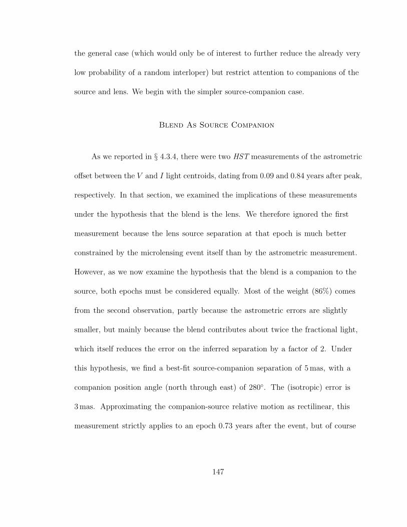
the general case (which would only be of interest to further reduce the already very

low probability of a random interloper) but restrict attention to companions of the

source and lens. We begin with the simpler source-companion case.

Blend As Source Companion

As we reported in § 4.3.4, there were two HST measurements of the astrometric

offset between the V and I light centroids, dating from 0.09 and 0.84 years after peak,

respectively. In that section, we examined the implications of these measurements

under the hypothesis that the blend is the lens. We therefore ignored the first

measurement because the lens source separation at that epoch is much better

constrained by the microlensing event itself than by the astrometric measurement.

However, as we now examine the hypothesis that the blend is a companion to the

source, both epochs must be considered equally. Most of the weight (86%) comes

from the second observation, partly because the astrometric errors are slightly

smaller, but mainly because the blend contributes about twice the fractional light,

which itself reduces the error on the inferred separation by a factor of 2. Under

this hypothesis, we find a best-fit source-companion separation of 5 mas, with a

companion position angle (north through east) of 280. The (isotropic) error is

3 mas. Approximating the companion-source relative motion as rectilinear, this

measurement strictly applies to an epoch 0.73 years after the event, but of course

147

the intrinsic source-companion relative motion must be very small compared to the

errors in this measurement.

There would be nothing unusual about such a source-companion projected

separation, roughly 40 ± 25 AU in physical units. Indeed, the local G-star binary

distribution function peaks close to this value (Duquennoy & Mayor 1991).

The derived separation is also marginally consistent with the companion

generating a xallarap signal that mimics the parallax signal in our dominant

interpretation. The semi-major axis of the orbit would have to be about 0.8 AU to

mimic the 1-year period of the Earth, which corresponds to a maximum angular

separation of about 100 µas, which is compatible with the astrometric measurements

at the 1.6 σ level.

Another potential constraint comes from comparing the color difference with

the magnitude difference of the source and blend. We find that the source is about

0.5 ± 0.5 mag too bright to be on the same main sequence. However, first, this is

only a 1σ difference, which is not significant. Second, both the sign and magnitude

of the difference are compatible with the source being a slightly evolved turnoff star,

which is consistent with its color.

The only present evidence against the source-companion hypothesis is that the

astrometric offset between V and I HST images changes between the two epochs,

and that the direction and amplitude of this change is consistent with other evidence

148

of the proper motion of the lens. Since this is only a P = 1.7% effect, it cannot be

regarded as conclusive. However, additional HST observations at a later epoch could

definitively confirm or rule out this hypothesis.

Blend As A Lens Companion

A similar, but somewhat more complicated line of reasoning essentially rules

out the hypothesis that the blend is a companion to the lens, at least if the lens is

luminous. The primary difference is that the event itself places very strong lower

limits on how close a companion can be to the lens.

A companion with separation (in units of θE) d ≫ 1 induces a Chang-Refsdal

(1979) caustic, which is fully characterized by the gravitational shear γ = q/d2. We

find that the light-curve distortions induced by this shear would be easily noticed

unless γ < 0.0035, that is,

γ =qc

d2c

=qcθ

2E

θ2c

< 0.0035, (4.29)

where qc = Mc/M is the ratio of the companion mass to the lens mass and dc = θc/θE

is the ratio of the lens-companion separation to the Einstein radius. Equivalently,

θc > 19(

qc

1.3

)1/2

θE. (4.30)

149

Here, we have normalized qc to the minimum mass ratio required for the companion

to dominate the light assuming that both are main-sequence stars. (We will also

consider completely dark lenses below).

We now show that equation (4.30) is inconsistent with the astrometric data. If a

lens companion is assumed to generate the blend light, then essentially the same line

of reasoning given in § 4.3.7 implies that 0.73 years after the event, this companion

lies 5 mas from the source, at position angle 280 and with an isotropic error of 3

mas. The one wrinkle is that we should now take account of the relative-parallax

term in equation (4.15), whereas this was identically zero (and so was ignored) for

the source-companion case. However, this term is only about 1.8πrel and hence is

quite small compared to the measurement errors for typical πrel ∼< 0.2mas. We will

therefore ignore this term in the interest of simplicity, except when we explicitly

consider the case of large πrel further below.

Of course, the lens itself moves during this interval. From the parallax

measurement alone (i.e. without attributing the V/I astrometric displacement to

lens motion), it is known that the lens is moving in the same general direction,

i.e., with position angle roughly 210. In assessing the amplitude of this motion we

consider only the constraints from finite-source effects (and ignore the astrometric

displacement). These constraints yield a hard lower limit on θE (from lack of

pronounced finite-source effects) of θE > 0.6 mas, which corresponds to a proper

motion µ = 3.1 mas yr−1. At this extreme value (and allowing for 2σ uncertainty

150

in the direction of lens motion as well in the measurement of the companion

position), the maximum lens-companion separation is 11.4 mas (i.e., 19 θE),

which is just ruled out by equation (4.30). At larger θE, the lens-companion

scenario is excluded more robustly. For example, in the limit of large θE, we have

θc = µ × 0.73 yr = θE(0.73 yr/tE) = 3.9θE, which is clearly ruled out by equation

(4.30).

Then we note that any scenario involving values of πrel that are large enough

that they cannot be ignored in this analysis (πrel ∼> 0.5 mas), must also have very

large θE = πrel/πE ∼> 1 mas, a regime in which the lens-companion is easily excluded.

The one major loophole to this argument is that the lens may be a stellar

remnant (white dwarf, neutron star, or black hole), in which case it could be more

massive than the companion despite the latter’s greater luminosity.

4.3.8. Xallarap Effects and Binary Source

Binary source motion can give rise to distortions of the light curve, called

“xallarap” effects. One can always find a set of xallarap parameters to perfectly

mimic parallax distortions caused by the Earth’s motion (Smith et al. 2003).

However, it is a priori unlikely for the binary source to have such parameters, so

if the parallax signal is real, one would expect the xallarap fits to converge to the

Earth parameters. For simplicity, we assume that the binary source is in circular

151

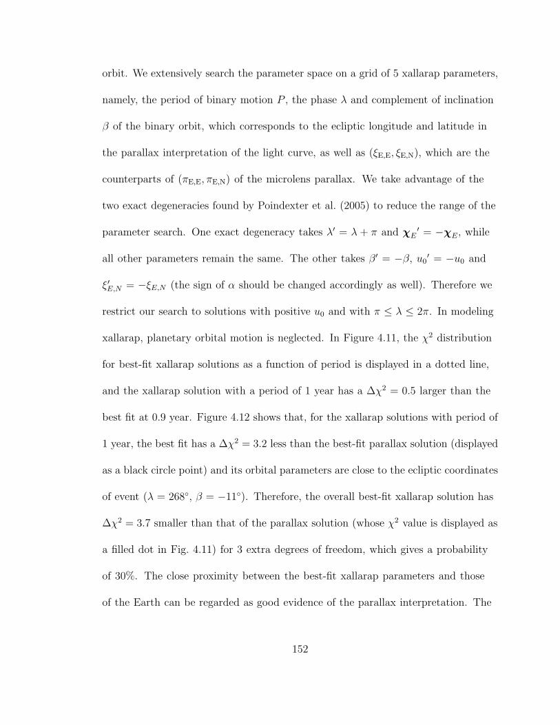
orbit. We extensively search the parameter space on a grid of 5 xallarap parameters,

namely, the period of binary motion P , the phase λ and complement of inclination

β of the binary orbit, which corresponds to the ecliptic longitude and latitude in

the parallax interpretation of the light curve, as well as (ξE,E, ξE,N), which are the

counterparts of (πE,E, πE,N) of the microlens parallax. We take advantage of the

two exact degeneracies found by Poindexter et al. (2005) to reduce the range of the

parameter search. One exact degeneracy takes λ′ = λ + π and χE′ = −χE, while

all other parameters remain the same. The other takes β′ = −β, u0′ = −u0 and

ξ′E,N = −ξE,N (the sign of α should be changed accordingly as well). Therefore we

restrict our search to solutions with positive u0 and with π ≤ λ ≤ 2π. In modeling

xallarap, planetary orbital motion is neglected. In Figure 4.11, the χ2 distribution

for best-fit xallarap solutions as a function of period is displayed in a dotted line,

and the xallarap solution with a period of 1 year has a ∆χ2 = 0.5 larger than the

best fit at 0.9 year. Figure 4.12 shows that, for the xallarap solutions with period of

1 year, the best fit has a ∆χ2 = 3.2 less than the best-fit parallax solution (displayed

as a black circle point) and its orbital parameters are close to the ecliptic coordinates

of event (λ = 268, β = −11). Therefore, the overall best-fit xallarap solution has

∆χ2 = 3.7 smaller than that of the parallax solution (whose χ2 value is displayed as

a filled dot in Fig. 4.11) for 3 extra degrees of freedom, which gives a probability

of 30%. The close proximity between the best-fit xallarap parameters and those

of the Earth can be regarded as good evidence of the parallax interpretation. The

152

slight preference of xallarap could simply be statistical fluctuation or reflect low-level

systematics in the light curve (commonly found in the analysis by Poindexter et al.

2005).

We also devise another test on the plausibility of xallarap. In § 4.3.5, we argued

that the blend is unlikely to be a random interloper unrelated to either the source or

the lens. If the source were in a binary, then the blend would naturally be explained

as the companion of the source star. Then from the blend’s position on the CMD,

its mass would be mc ∼ 0.9 M⊙. By definition, ξE is the size of the source’s orbit as

in the units of rE (the Einstein radius projected on the source plane),

ξE =as

rE

=amc

(mc + ms)rE

, (4.31)

where a is the semimajor axis of the binary orbit, and ms and mc are the masses of

the source and its companion, respectively. Then we apply Kepler’s Third Law:

(

P

yr

)2 m3c

M⊙(mc + ms)2=(

ξErE

AU

)3

. (4.32)

Once the masses of the source and companion are known, the product of ξE and

rE are determined for a given binary orbital period P . And in the present case,

rE/AU = θEDs = θ∗/ρDs = 4.5 × 10−3/ρ. By adopting ms = 1M⊙, mc = 0.9M⊙, for

each set of P and ρ, there is a uniquely determined ξE from equation (4.32). We then

apply this constraint in the xallarap fitting for a series of periods. The minimum χ2s

for each period from the fittings are shown in solid line in Figure 4.11. The best-fit

153

solution has ∆χ2 ∼ 1.0 less than the best-fit parallax solution for two extra degrees

of freedom. Although as compared to the test described in the previous paragraph,

the current test implies a higher probability that the data are explained by parallax

(rather than xallarap) effects, it still does not rule out xallarap.

4.4. Summary and Future Prospects

Our primary interpretation of the OGLE-2005-BLG-071 data assumes that the

light-curve distortions are due to parallax rather than xallarap and that the blended

light is due to the lens itself rather than a companion to the source. Under these

assumptions, the lens is fairly tightly constrained to be a foreground M dwarf, with

mass M = 0.46 ± 0.04 M⊙ and distance Dl = 3.2 ± 0.4 kpc, which has thick-disk

kinematics (vLSR ∼ 103 km s−1). As we discuss below, future observations might

help to constrain its metallicity. The microlens modeling suffers from a well-known

wide-close binary degeneracy. The best-fit wide-binary solutions are slightly favored

over the close-binary solutions, however, from dynamical constraints on planetary

orbital motion, the physically allowed solutions are not distinguishable within 1 σ.

For the wide-binary model, we obtain a planet of mass Mp = 3.8 ± 0.4 MJupiter

at projected separation r⊥ = 3.6 ± 0.2 AU. The planet then has an equilibrium

temperature of about T = 55 K, i.e. similar to Neptune. In the degenerate

154

close-binary solutions, the planet is closer to the star and so hotter, and the

estimates are: Mp = 3.4 ± 0.4 MJupiter, r⊥ = 2.1 ± 0.1 AU and T ∼ 71 K.

As we have explored in considerable detail, it is possible that one or both of

these assumptions is incorrect. However, future astrometric measurements that are

made after the lens and source have had a chance to separate, will largely resolve

both ambiguities. Moreover, such measurements will put much tighter constraints

on the metallicity of the lens (assuming that it proves to be the blended light).

First, the astrometric measurements made 0.84 yr after the event detected

motion suggests that there was still 1.7% chance that the blend did not move relative

to the source. A later measurement that detected this motion at higher confidence

would rule out the hypothesis that the blend is a companion to the source. We

argued in § 4.3.7 that the blend could not be a companion to a main-sequence

lens. Therefore, the only possibilities that would remain are that the lens is the

blend, that the lens is a remnant (e.g., white dwarf), or that the blend is a random

interloper (probability < 10−3). As we briefly summarize below, a future astrometric

measurement could strongly constrain the remnant-lens hypothesis as well.

Of course, it is also possible that future astrometry will reveal that the blend

does not moving with respect to the source, in which case the blend would be a

companion to the source. Thus, either way, these measurements would largely

resolve the nature of the blended light.

155

Second, by identifying the nature of blend, these measurements will largely,

but not entirely, resolve the issue of parallax vs. xallarap. If the blend proves not to

be associated with the source, then any xallarap-inducing companion would have to

be considerably less luminous, and so (unless it were a neutron star) less massive

than the mc = 0.9 M⊙ that we assumed in evaluating equation (4.32). Moreover,

stronger constraints on rE (rhs of eq. [4.32]) would be available from the astrometric

measurements. Hence, the xallarap option would be either excluded or very strongly

constrained by this test.

On the other hand, if the blend were confirmed to be a source companion, then

essentially all higher order constraints on the nature of the lens would disappear.

The parallax “measurement” would then very plausibly be explained by xallarap,

while the “extra information” about θE that is presently assumed to come from the

blend proper-motion measurement would likewise evaporate.

These considerations strongly argue for making a future high-precision

astrometric measurement. Recall that in the HST measurements reported in § 4.3.5,

the source and blend were not separately resolved: the relative motion was inferred

from the offset between the V and I centroids, which are displaced because the source

and blend have different colors. Due to its well-controlled PSF, HST is capable of

detecting the broadening of the PSF even if the separation of the lens and source is

a fraction of the FWHM. Assuming that the proper motion is µgeo ∼ 4.4 mas yr−1,

and based on our simulations in § 4.3.5, such broadening would be confidently

156

detectable about 5 years after the event (see also Bennett et al. 2007 for analytic

PSF broadening estimates). Ten years after the event, the net displacement would

be ∼ 40 mas. This compares to a diffraction limited FWHM of 40 mas for H band on

a ground-based 10m telescope and would therefore enable full resolution. The I −H

color of the source is extremely well determined (0.01 mag) from simultaneous I and

H data taken during the event from the CTIO/SMARTS 1.3m in Chile. Hence,

the flux allocation of the partially or fully resolved blend and source stars would

be known. The direct detection of a partially or fully resolved lens will provide

precise photometric and astrometry measurements (see Kozlowski et al. 2007 for one

such example), which will enable much tighter constraints on the mass, distance

and projected velocity of the lens. It also opens up the possibility of determining

the metallicity of the host star by taking into account both non-photometric and

photometric constraints. If, as indicated by the projected velocity measurement, it

is a thick-disk star, then it will be one of the few such stars found to harbor a planet

(Haywood 2008).

As remarked above, a definitive detection of the blend’s proper motion would

still leave open the possibility that it was a companion to the lens, and not the

lens itself. In this case, the lens would have to be a remnant. Without going into

detail, the astrometric measurement would simultaneously improve the blend color

measurement as well as giving a proper-motion estimate (albeit with large errors

because the blend-source offset at the peak of the event would then not be known).

157

It could then be asked whether the parallax, proper-motion, and photometric

data could be consistently explained by any combination of remnant lens and

main-sequence companion. This analysis would depend critically on the values of

the measurements, so we do not explore it further here. We simply note that this

scenario could also be strongly constrained by future astrometry.

4.5. Discussion

With the measurements presented here, and the precision with which these

measurements allow us to determine the properties of the planet OGLE-2005-BLG-

071Lb and its host, it is now possible to place this system in the context of similar

planetary systems discovered by radial velocity (RV) surveys. Of course, the kind

of information that can be inferred about the planetary systems discovered via RV

differs somewhat from that presented here. For example, for planets discovered via

RV, it is generally only possible to infer a lower limit to the planet mass, unless

the planets happen to transit or produce a detectable astrometric signal. Mutatis

mutandis, for planets discovered via microlensing, it is generally only possible to

measure the projected separation at the time of the event, even in the case for which

the microlensing mass degeneracy is broken as it is here (although see Gaudi et al.

2008).

158

With these caveats in mind, we can compare the properties of OGLE-2005-

BLG-071Lb and its host star with similar RV systems. It is interesting to note that

the fractional uncertainties in the host mass and distance of OGLE-2005-BLG-071Lb

are comparable to those of some of the systems listed in Table 4.6.

OGLE-2005-BLG-071Lb is one of only eight Jovian-mass (0.2MJupiter <

Mp < 13MJupiter) planets that have been detected orbiting M dwarf hosts (i.e.,

M∗ < 0.55 M⊙) (Marcy et al. 1998, 2001; Delfosse et al. 1998; Butler et al. 2006;

Johnson et al. 2007b; Bailey et al. 2008). Table 4.6 summarizes the planetary

and host-star properties of the known M dwarf/Jovian-mass planetary systems.

OGLE-2005-BLG-071Lb is likely the most massive known planet orbiting an M

dwarf.

As suggested by the small number of systems listed in Table 4.6, and shown

quantitatively by several recent studies, the frequency of relatively short-period

P ∼< 2000 days, Jupiter-mass companions to M dwarfs appears to be ∼ 3 − 5 times

lower than such companions to FGK dwarfs (Butler et al. 2006; Endl et al. 2006;

Johnson et al. 2007b; Cumming et al. 2008). This paucity, which has been shown

to be statistically significant, is expected in the core-accretion model of planet

formation, which generally predicts that Jovian companions to M dwarfs should be

rare, since for lower mass stars, the dynamical time at the sites of planet formation is

longer, whereas the amount of raw material available for planet formation is smaller

(Laughlin et al. 2004; Ida & Lin 2005; Kennedy & Kenyon 2008, but see Kornet

159

et al. 2006). Thus, these planets typically do not reach sufficient mass to accrete a

massive gaseous envelope over the lifetime of the disk. Consequently, such models

also predict that in the outer regions of their planetary systems, lower mass stars

should host a much larger population of ‘failed Jupiters,’ cores of mass ∼< 10 M⊕

(Laughlin et al. 2004; Ida & Lin 2005). Such a population was indeed identified

based on two microlensing planet discoveries (Beaulieu et al. 2006; Gould et al.

2006).

Our detection of a ∼ 4 MJupiter companion to an M dwarf may therefore present

a difficulty for the core-accretion scenario. While we do not have a constraint on the

metallicity of the host, the fact that it is likely a member of the thick disk suggests

that its metallicity may be subsolar. If so, this would pose an additional difficulty for

the core-accretion scenario, which also predicts that massive planets should be rarer

around metal-poor stars (Ida & Lin 2004), as has been demonstrated observationally

(Santos et al. 2004; Fischer & Valenti 2005). This might imply that a different

mechanism is responsible for planet formation in the OGLE-2005-BLG-071L system,

such as the gravitational instability mechanism (Boss 2002, 2006).

One way to escape these potential difficulties is if the host lens is actually a

stellar remnant, such as white dwarf. The progenitors of remnants are generally

more massive stars, which are both predicted (Ida & Lin 2005; Kennedy & Kenyon

2008) and observed (Johnson et al. 2007a,b) to have a higher incidence of massive

planets. As we discussed above, future astrometric measurements could constrain

160

both the low-metallicity and remnant-lens hypotheses. These measurements are

therefore critical.

Although it is difficult to draw robust conclusions from a single system,

there are now four published detections of Jovian-mass planetary companions

with microlensing (Bond et al. 2004; Gaudi et al. 2008), and several additional

such planets have been detected that are currently being analyzed. It is therefore

reasonable to expect several detections per year (Gould 2009), and thus that it will

soon be possible to use microlensing to constrain the frequency of massive planetary

companions. These constraints are complementary to those from RV, since the

microlensing detection method is less biased with respect to host star mass (Gould

2000a), and furthermore probes a different region of parameter space, namely cool

planets beyond the snow line with equilibrium temperatures similar to the giant

planets in our solar system (see, e.g. Gould et al. 2007 and Gould 2009).

161

RoboNet FTN R

PLANET Canopus I

MOA I

I

I

Clear

V

I

ClearOGLE V

OGLE I

3479 3480 3481 3482 348316

15.8

15.6

15.4

15.2

15

Fig. 4.1.— Main panel: all available ground-based data of the microlensing eventOGLE-2005-BLG-071. HST ACS HRC observations in F814W and F555W weretaken at two epochs, once when the source was magnified by A ∼ 2 (arrow), andagain at HJD = 2453788.2 (at baseline). Planetary models that include (solid) andexcludes (dotted) microlens parallax are shown. Zoom at bottom: triple-peak featurethat reveals the presence of the planet. Each of the three peaks corresponds to thesource passing by a cusp of the central caustic induced by the planet. Upper inset:trajectory of the source relative to the lens system in the units of angular Einsteinradius θE. The lens star is at (0, 0), and the star-planet axis is parallel to the x-axis.The best-fit angular size of the source star in units of θE is ρ ∼ 0.0006, too small tobe resolved in this figure.

162

Fig. 4.2.— Probability contours (∆χ2 = 1, 4) of microlens parallax parametersderived from MCMC simulations for wide-binary (in solid line) and close-binary (in adashed line) solutions. Fig. 2 and eq. (12) in Gould (2004) imply that πE,⊥ is definedso that πE,‖ and πE,⊥ form a right-handed coordinate system.

163

Fig. 4.3.— CMD for the OGLE-2005-BLG-071 field. Black dots are the stars withthe OGLE I-band and V -band observations. The red point and green points show thecenter of red clump and the source, respectively. The errors in their fluxes and colorsare too small to be visible on the graph. Cyan points are the stars in the ACS field,which are photometrically aligned with OGLE stars using 10 common stars. Themagenta point with error bars show the color and magnitude of the blended light.

164

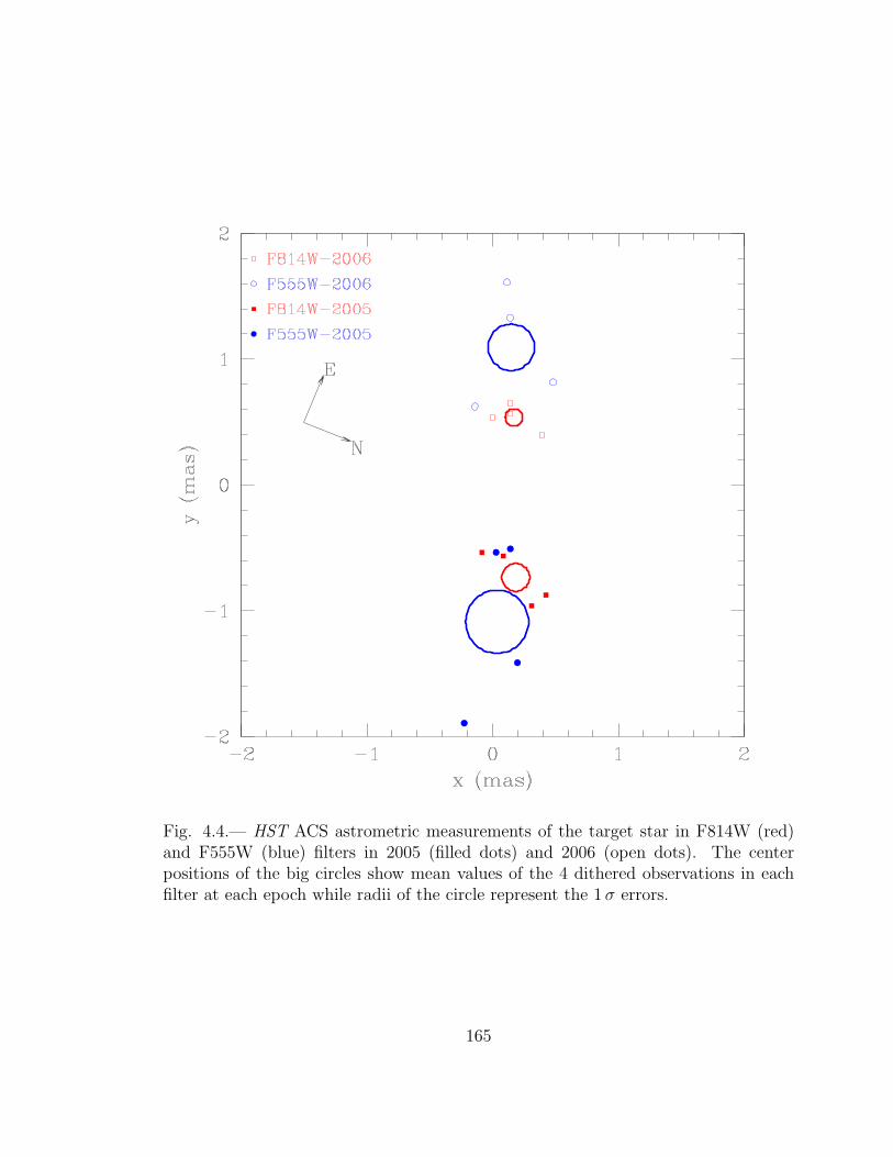
Fig. 4.4.— HST ACS astrometric measurements of the target star in F814W (red)and F555W (blue) filters in 2005 (filled dots) and 2006 (open dots). The centerpositions of the big circles show mean values of the 4 dithered observations in eachfilter at each epoch while radii of the circle represent the 1σ errors.

165

finite-sourceastrometryjoint

wide

wideparallaxjoint

finite-sourceastrometryjoint

close

closeparallaxjoint

Fig. 4.5.— Upper two panels show posterior probability contours at ∆χ2 = 1 (solidline) and 4 (dotted line) for relative lens-source proper motion µgeo. The left panelis for wide-binary solutions and the right one is for close-binary. The green contoursshow the probability distributions constrained by the finite-source effects. The blackcontours are derived from HST astrometry measurements assuming πrel = 0.2 mas.The red contours show the joint probability distributions from both constraints. Thelower two panels show the posterior probability distribution of the position angle φµ

geo

of the relative lens-source proper motion for wide-binary and close-binary solutions,respectively. The histogram in red is derived from the red contours of joint probabilityfor finite source and astrometry constraints in the upper panel. The blue histogramrepresents that of the microlens parallax. They mildly disagree at 2.5σ.

166

Fig. 4.6.— Differences between OGLE V and HST F555W magnitudes for thematched stars are plotted against their V magnitudes measured by OGLE. Tocalculate the offset, we add a 0.017 mag “cosmic error” in quadrature to each point inorder to reduce χ2/dof to unity. The open circles represent the stars used to establishthe final transformation, and the filled point shows an “outlier”.

167

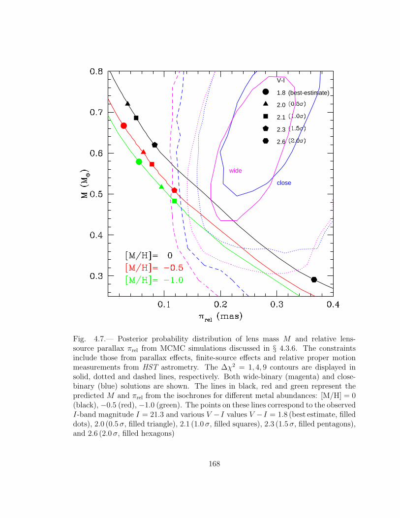
wide

close

V-I

1.8 (best-estimate)

2.0

2.1

2.3

2.6

Fig. 4.7.— Posterior probability distribution of lens mass M and relative lens-source parallax πrel from MCMC simulations discussed in § 4.3.6. The constraintsinclude those from parallax effects, finite-source effects and relative proper motionmeasurements from HST astrometry. The ∆χ2 = 1, 4, 9 contours are displayed insolid, dotted and dashed lines, respectively. Both wide-binary (magenta) and close-binary (blue) solutions are shown. The lines in black, red and green represent thepredicted M and πrel from the isochrones for different metal abundances: [M/H] = 0(black), −0.5 (red), −1.0 (green). The points on these lines correspond to the observedI-band magnitude I = 21.3 and various V −I values V −I = 1.8 (best estimate, filleddots), 2.0 (0.5 σ, filled triangle), 2.1 (1.0 σ, filled squares), 2.3 (1.5 σ, filled pentagons),and 2.6 (2.0 σ, filled hexagons)

168

Fig. 4.8.— Posterior probability distribution of lens mass M and relative lens-sourceparallax πrel from MCMC simulations assuming that the blended light comes fromthe lens star. The ∆χ2 = 1, 4 contours are displayed in a solid line for wide solutions,and in a dotted line for close solutions.

169

Fig. 4.9.— Probability contours of projected velocity r⊥γ (defined in Appendix C)in the units of vc,⊥ for both close-binary (upper panel) and wide-binary (lower panel)solutions. All the solutions that are outside the dotted circle are physically rejected asthe velocities exceed the escape velocity of the system. The boundary in a solid lineinside the dotted circle encloses the solutions for which circular orbits are allowed.

170

Fig. 4.10.— Probability distributions of planetary parameters (semimajor axis a,equilibrium temperature, cosine of the inclination, and amplitude of radial velocity ofthe lens star) from MCMC realizations assuming circular orbital motion. Histogramsin black and red represent the close-binary and wide-binary solutions, respectively.Dotted and dashed histograms represent the two degenerate solutions for each MCMCrealization discussed in Appendix C.

171

Fig. 4.11.— χ2 distributions for best-fit xallarap solutions at fixed binary-sourceorbital periods P . The solid and dotted lines represent xallarap fits with and withoutdynamical constraints described in § 4.3.8. The best-fit parallax solution is shown asa filled dot at period of 1 year. All of the fits shown in this figure assume no planetaryorbital motion.

172

Fig. 4.12.— Results of xallarap fits by fixing binary orbital phase λ and complementof inclination β at period P = 1 yr and u0 > 0. The plot is color-coded for solutionswith ∆χ2 within 1 (black), 4 (red), 9 (green), 16 (blue), 25 (magenta), 49 (yellow)of the best fit. The Earth parameters are indicated by black circles. Because of aperfect symmetry (u0 → −u0 and α → −α), the upper black circle represents Earthparameter (λ = 268, β = −11) for the case u0 < 0. Comparison of parallax withxallarap must be made with the better of the two, that is, the lower one.

173

Model t0 u0 tE d q α ρ πE,N πE,E ω d/d

χ2 (HJD’) (day) ×103 (deg) ×104 (yr−1) (yr−1)

Wide+ 3480.7024 0.0282 71.1 1.306 7.5 273.63 3.9 -0.30 -0.26 -1.328 -0.256

1345.0 +0.0058−0.0054

+0.0008−0.0009

+2.3−2.4

+0.002−0.004 ±0.2 +0.16

−0.15+1.8−2.7

+0.24−0.28 ±0.05 +0.274

−0.165+0.134−0.129

Wide− 3480.7028 -0.0283 70.6 1.307 7.5 86.21 3.9 -0.34 -0.26 1.117 -0.277

1345.3 +0.0054−0.0056

+0.0010−0.0008 ±2.2 +0.003

−0.004 ±0.3 +0.13−0.16

+1.8−2.6

+0.30−0.23 ±0.05 +0.130

−0.293+0.152−0.113

Close+ 3480.6789 0.0239 70.1 0.763 6.9 274.27 3.1 -0.36 -0.27 0.301 0.502

1345.8 +0.0055−0.0043

+0.0009−0.0007

+2.1−2.4

+0.004−0.006 ±0.3 +0.25

−0.36+1.7−2.5

+0.24−0.27 ±0.05 +0.486

−0.788+0.148−0.101

Close− 3480.6799 -0.0241 69.2 0.762 6.9 85.53 2.7 -0.33 -0.26 -0.405 0.528

1345.2 +0.0042−0.0051

+0.0009−0.0007

+2.3−1.9

+0.004−0.006 ±0.3 +0.39

−0.26 ±2.2 +0.28−0.26 ±0.05 +0.696

−0.622+0.127−0.118

Table 4.1. OGLE-2005-BLG-071 Light Curve Parameter Estimations From Markov chain Monte

Carlo Simulations A (Part 1).

174

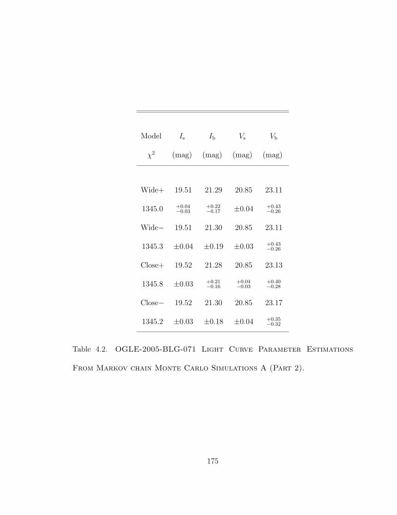
Model Is Ib Vs Vb

χ2 (mag) (mag) (mag) (mag)

Wide+ 19.51 21.29 20.85 23.11

1345.0 +0.04−0.03

+0.22−0.17 ±0.04 +0.43

−0.26

Wide− 19.51 21.30 20.85 23.11

1345.3 ±0.04 ±0.19 ±0.03 +0.43−0.26

Close+ 19.52 21.28 20.85 23.13

1345.8 ±0.03 +0.21−0.16

+0.04−0.03

+0.40−0.28

Close− 19.52 21.30 20.85 23.17

1345.2 ±0.03 ±0.18 ±0.04 +0.35−0.32

Table 4.2. OGLE-2005-BLG-071 Light Curve Parameter Estimations

From Markov chain Monte Carlo Simulations A (Part 2).

175

Model t0 u0 tE d q α ρ πE,N πE,E ω d/d

χ2 (HJD’) (day) ×103 (deg) ×104 (yr−1) (yr−1)

Wide+ 3480.7015 0.0287 69.3 1.305 7.7 273.67 6.1 -0.02 -0.22 -1.242 -0.283

1353.4 +0.0050−0.0059 ±0.0007 +1.6

−1.7+0.003−0.005 ±0.2 +0.17

−0.11 ±0.4 ±0.12 ±0.03 +0.321−0.125 ±0.129

Wide− 3480.7012 -0.0287 69.2 1.305 7.7 86.29 6.0 0.02 -0.21 1.193 -0.293

1353.3 +0.0052−0.0060 ±0.0007 +1.7

−1.8+0.002−0.005 ±0.2 +0.12

−0.15+0.5−0.3

+0.10−0.13 ±0.03 +0.127

−0.342+0.131−0.121

Close+ 3480.6792 0.0245 68.3 0.763 7.0 274.38 6.0 -0.01 -0.22 0.415 0.569

1355.5 +0.0041−0.0051

+0.0005−0.0006 ±1.6 +0.003

−0.006+0.3−0.2

+0.23−0.39 ±0.4 +0.12

−0.15 ±0.02 +0.503−0.744

+0.112−0.130

Close− 3480.6793 -0.0245 68.2 0.762 7.1 85.63 6.0 0.04 -0.22 -0.179 0.561

1355.5 +0.0042−0.0051 ±0.0006 +1.8

−1.5+0.004−0.006 ±0.3 +0.46

−0.24 ±0.4 +0.09−0.16 ±0.03 +0.703

−0.722+0.126−0.112

Table 4.3. OGLE-2005-BLG-071 Light Curve Parameter Estimations From Markov chain Monte

Carlo Simulations B (Part 1).

176

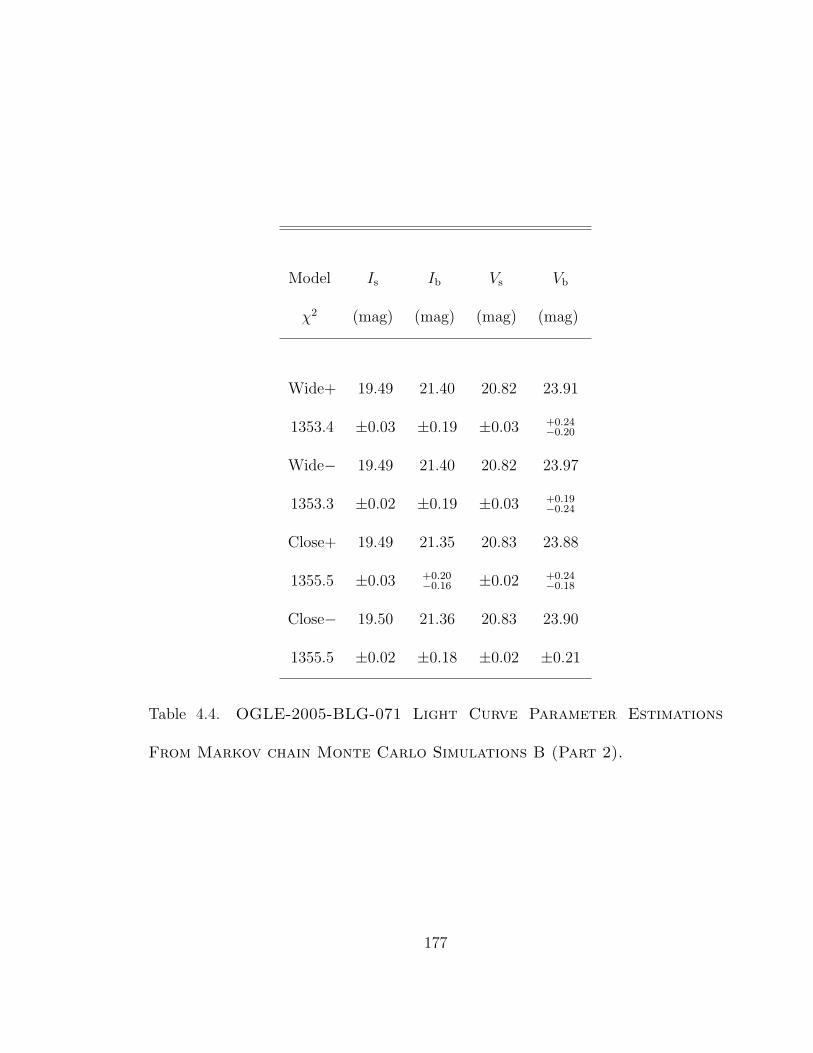
Model Is Ib Vs Vb

χ2 (mag) (mag) (mag) (mag)

Wide+ 19.49 21.40 20.82 23.91

1353.4 ±0.03 ±0.19 ±0.03 +0.24−0.20

Wide− 19.49 21.40 20.82 23.97

1353.3 ±0.02 ±0.19 ±0.03 +0.19−0.24

Close+ 19.49 21.35 20.83 23.88

1355.5 ±0.03 +0.20−0.16 ±0.02 +0.24

−0.18

Close− 19.50 21.36 20.83 23.90

1355.5 ±0.02 ±0.18 ±0.02 ±0.21

Table 4.4. OGLE-2005-BLG-071 Light Curve Parameter Estimations

From Markov chain Monte Carlo Simulations B (Part 2).

177

Model M πrel Dl µN µE θE Mp r⊥

χ2 M⊙ mas kpc mas yr−1 mas yr−1 mas MJupiter AU

Wide+ 0.46 0.19 3.2 -0.4 -4.3 0.84 3.8 3.6

1353.4 ±0.04 ±0.04 ±0.4 +2.7−3.1 ±0.3 +0.06

−0.04+0.3−0.4 ±0.2

Wide− 0.46 0.19 3.2 0.3 -4.3 0.85 3.8 3.6

1353.3 ±0.04 +0.04−0.03 ±0.4 +2.3

−3.6+0.3−0.2 ±0.05 +0.3

−0.4 ±0.2

Close+ 0.46 0.19 3.1 -2.6 -4.4 0.86 3.4 2.1

1355.5 ±0.04 +0.04−0.03 ±0.4 +4.8

−1.1 ±0.3 ±0.05 +0.3−0.4 ±0.1

Close− 0.46 0.20 3.1 -0.2 -4.4 0.87 3.4 2.1

1355.5 ±0.04 ±0.04 ±0.3 +3.6−3.4 ±0.3 ±0.04 ±0.3 ±0.1

Table 4.5. OGLE-2005-BLG-071 Derived Physical Parameters

178

Name M∗ Metallicity Dist. Mp P a Ref.

(M⊙) (pc) (MJup) (days) (AU)

GJ 876c 0.32 −0.12 4.660 0.6− 30.340 0.13030 1,2,3

±0.03 ±0.12 ±0.004 0.8 ±0.013

GJ 876b – – – 1.9− 60.940 0.20783 –

2.5 ±0.013

GJ 849b 0.49 0.16 8.8 0.82/ sin i 1890 2.35 4

±0.05 ±0.2 ±0.2 ±130

GJ 317b 0.24 −0.23 9.2 1.2/ sin i 692.9 0.95 5

±0.04 ±0.2 ±1.7 ±4

GJ 832b 0.45 ∼ −0.7 ∼ 4.93 0.64/ sin i 3416 3.4 6

±0.05 /-0.3 ±131 ±0.4

OGLE-2006 0.50 ? 1490 0.71 1830 2.3 7

-BLG-109Lb ±0.05 ? ±130 ±0.08 ±370 ±0.2

OGLE-2006 – – – 0.27 5100 4.6 –

-BLG-109Lc ±0.03 ±730 ±0.5

(cont’d)

Table 4.6. Jovian-mass Companions to M Dwarfs (M∗ < 0.55 M⊙)

179

Table 4.6—Continued

Name M∗ Metallicity Dist. Mp P a Ref.

(M⊙) (pc) (MJup) (days) (AU)

OGLE-2005 0.46 Subsolar?a 3300 3.8b – 3.6b,c This

-BLG-071Lb ±0.04 ±300 ±0.4 ±0.2 Paper

aWhile the metallicity of the OGLE-2005-BLG-071Lb host star is not directly

constrained by our data, its kinematics indicate it is likely a member of the metal-

poor thick disk.

bWe give the planet mass and projected separation for the wide solution, which

is favored by ∆χ2 = 2.1. The second, close solution has Mp = 3.4 ± 0.3 MJupiter

and r⊥ = 2.1 ± 0.1 AU.cWe give the the projected separation between the host and planet at the

time of event, which is the orbital parameter most directly constrained by our

observations. However, assuming a circular orbit, we infer that the semi-major

axis is likely only ∼ 10 − 20% larger [a(wide) ∼ 4.1AU, a(close) ∼ 2.5AU].

References. — (1)Rivera et al. 2005; (2)Bean et al. 2006; (3)Benedict et al.

2002; (4)Butler et al. 2006; (5) Johnson et al. 2007b (6) Bailey et al. 2008 (7)

Gaudi et al. 2008

180

Chapter 5

First Space-Based Microlens Parallax

Measurement: Spitzer Observations of

OGLE-2005-SMC-001

5.1. Introduction

In a visionary paper written more than 40 years ago, Refsdal (1966) argued

that two important but otherwise unmeasurable parameters of microlensing events

could be determined by simultaneously observing the event from the Earth and a

satellite in solar orbit. In modern language, these are the Einstein radius projected

onto the observer plane, rE, and the direction of lens-source relative proper motion.

Since the Einstein timescale, tE, is routinely measured for all events, these parameter

determinations are equivalent to knowing the projected relative velocity, v, whose

magnitude is simply v ≡ rE/tE. Here, rE ≡ AU/πE, tE = θE/µ, and

πE =

√

πrel

κM, θE =

√

κMπrel, (5.1)

181

where πE is the microlens parallax, M is the mass of the lens, θE is the angular

Einstein radius, πrel and µ are the lens-source relative parallax and proper motion,

respectively, and κ ≡ 4G/(c2AU).

The practical importance of this suggestion became clear when the MACHO

(Alcock et al. 1993) and EROS (Aubourg et al. 1993) collaborations reported the

detection of microlensing events toward the Large Magellanic Cloud (LMC). Over

the course of time, MACHO (Alcock et al. 1997, 2000) has found about 15 such

events and argued that these imply that about 20% of the Milky Way dark halo

is composed of compact objects (“MACHOs”), while EROS (Afonso et al. 2003;

Tisserand et al. 2006) has argued that their relative lack of such detections was

consistent with all the events being due to stars in the Milky Way disk or the

Magellanic Clouds (MCs) themselves. For any given individual event, it is generally

impossible to tell (with only a measurement of tE) where along the line of sight the

lens lies, so one cannot distinguish among the three possibilities: Milky Way disk,

Milky Way halo, or “self-lensing” in which the source and lens both lie in the same

external galaxy.

However, as Boutreux & Gould (1996) argued, measurement of v might allow

one to distinguish among these populations with good confidence: disk, halo, and

MC lenses typically have v values of 50, 300, and 2000 km s−1, respectively. The high

projected speed of MC lenses derives from the long “lever arm” that multiplies their

182

small local transverse speed by the ratio of the distances from the observer and the

lens to the source.

There are serious obstacles, both practical and theoretical to measuring v. One

obvious practical problem is simply launching a spacecraft with a suitable camera

into solar orbit. But the theoretical difficulties also place significant constraints on

the characteristics of that spacecraft. To understand these properly, one should

think in terms of the “microlens parallax” πE, whose magnitude is πE ≡ AU/rE

and whose direction is the same as v. Choosing a coordinate system whose x-axis

is aligned with the Earth-satellite separation at the peak of the event, we can write

πE = (πE,τ , πE,β). Then to good approximation,

πE = (πE,τ , πE,β) =AU

d⊥

(

∆t0tE

, ∆u0

)

, (5.2)

where d⊥ is the Earth-satellite separation (projected onto the plane of the sky), ∆t0

is the difference in time of event maximum as seen from the Earth and satellite,

and ∆u0 is the difference in dimensionless impact parameter (determined from the

maximum observed magnification).

Refsdal (1966) already realized that equation (5.2) implicitly contains a

four-fold degeneracy: while ∆t0/tE is unambiguously determined, there are four

different values of ∆u0 that depend on whether the individual impact parameters are

positive or negative (on one side of the lens or the other; see Fig. 2 of Gould 1994b).

183

In fact, the situation is considerably worse than this. While t0 is usually measured

very precisely in individual microlensing events, u0 typically has much larger errors

because it is strongly correlated with three other parameters, the timescale, tE, the

source flux fs, and the blended flux, fb. For a satellite separated by d⊥ ∼ 0.2 AU, and

a projected Einstein radius rE ∼ 5 AU, errors in the impact-parameter determinations

of only σ(u0) ∼ 2% would lead to fractional errors σ(πE)/πE ∼√

2σ(u0)rE/d⊥ ∼ 70%.

However, Gould (1995) showed that if the two cameras had essentially identical

spectral responses and similar point-spread-functions, so that one knew a priori that

the blended light was virtually identical for the Earth and satellite measurements,

then the error in ∆u0 would be reduced far below the individual errors in u0, making

the parallax determination once again feasible.

Unfortunately, this trick cannot be used on Spitzer, the first general purpose

camera to be placed in solar orbit. The shortest wavelength at which Spitzer operates

is the L band (3.6 µm), implying that the camera’s sensitivity cannot be duplicated

from the ground, because of both higher background and different throughput as a

function of wavelength.

In principle, microlens parallaxes can also be measured from the ground.

As with space-based parallaxes, one component of πE can generally be measured

much more precisely than the other. For most events, tE ≪ yr, and for these the

Earth’s acceleration can be approximated as constant during the event. To the

degree that this acceleration is aligned (anti-aligned) with the lens-source relative

184

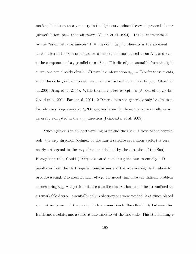
motion, it induces an asymmetry in the light curve, since the event proceeds faster

(slower) before peak than afterward (Gould et al. 1994). This is characterized

by the “asymmetry parameter” Γ ≡ πE · α = πE,‖α, where α is the apparent

acceleration of the Sun projected onto the sky and normalized to an AU, and πE,‖

is the component of πE parallel to α. Since Γ is directly measurable from the light

curve, one can directly obtain 1-D parallax information πE,‖ = Γ/α for these events,

while the orthogonal component πE,⊥ is measured extremely poorly (e.g., Ghosh et

al. 2004; Jiang et al. 2005). While there are a few exceptions (Alcock et al. 2001a;

Gould et al. 2004; Park et al. 2004), 2-D parallaxes can generally only be obtained

for relatively long events tE ∼> 90 days, and even for these, the πE error ellipse is

generally elongated in the πE,⊥ direction (Poindexter et al. 2005).

Since Spitzer is in an Earth-trailing orbit and the SMC is close to the ecliptic

pole, the πE,τ direction (defined by the Earth-satellite separation vector) is very

nearly orthogonal to the πE,‖ direction (defined by the direction of the Sun).

Recognizing this, Gould (1999) advocated combining the two essentially 1-D

parallaxes from the Earth-Spitzer comparison and the accelerating Earth alone to

produce a single 2-D measurement of πE. He noted that once the difficult problem

of measuring πE,β was jettisoned, the satellite observations could be streamlined to

a remarkable degree: essentially only 3 observations were needed, 2 at times placed

symmetrically around the peak, which are sensitive to the offset in t0 between the

Earth and satellite, and a third at late times to set the flux scale. This streamlining is

185

important from a practical point of view because Target-of-Opportunity (ToO) time

on Spitzer incurs a large penalty. Gould (1999) noted that the components of πE

measured by the two techniques were not exactly orthogonal but argued (incorrectly

as it turns out) that this had no significant consequences for the experiment. We

return to this point below.

Here we analyze Spitzer and ground-based observations of the microlensing

event OGLE-2005-SMC-001 to derive the first microlens parallax measurement using

this technique.

5.2. Observations

On 2005 July 9 (HJD′ ≡ HJD-2450000 = 3561.37), the OGLE-III Early

Warning System (EWS, Udalski 2003) alerted the astronomical community that

OGLE-2005-SMC-001 (αJ2000.0 = 0h40m28.s5, δJ2000.0 = −7344′46.1′′) was a probable

microlensing event, approximately 23 days (and seven observations) into the 2005

OGLE-III observing season for the SMC. In fact, the EWS issued an internal alert

five days earlier, when there were only three 2005 points, but the OGLE team reacted

cautiously because of the high rate of questionable alerts toward the SMC and

because the source lies projected against a background galaxy, making it a potential

supernova candidate. However, the event shows a modest, but unambiguous rise 140

days earlier, at the end of the 2004 season, which is inconsistent with a supernova,

186

and the unmagnified source sits right in the middle of the red giant clump on

the color-magnitude diagram (CMD), with (V − I, I) = (0.92, 18.4). Moreover,

the light curve is achromatic. These factors convinced us that this was genuine

microlensing, leading us to exercise our Spitzer ToO option, which consisted of

three 2-hr observations: two placed symmetrically around the peak and one at the

baseline. Once this decision was made, OGLE increased its density of coverage to

3–5 I-band observations per clear night. OGLE observations were obtained using

the 1.3 m Warsaw telescope at Las Campanas Observatory in Chile, operated by

the Carnegie Institution of Washington. The photometry was reduced using the

standard OGLE-III data pipeline (Udalski 2003) based on the image subtraction

technique, DIA (Wozniak 2000). Also many V -band observations were obtained

during the event for monitoring achromaticity. There are Spitzer observations at

four epochs (not three, as originally envisaged). These were centered at 2005 July

15 UT 20:02:40, 2005 August 25 UT 12:44:25, 2005 September 15 UT 20:13:53,

and 2005 November 29 UT 10:24:40. The first, third, and fourth observations each

lasted 2 hr and consisted of two sets of about 100 dithered exposures, each of 26.8

s. The second observation (in August) was 1 hr, consisting of one set of 99 dithered

exposures, each of 26.8 s. It was obtained with director’s discretionary time (DDT).

All four were carried out simultaneously at 3.6 and 5.8 µm. However, the third

observation (which took place at relatively high magnification) was supplemented by

30 minutes of very short exposures in all four Infrared Array Camera (IRAC) filters

187

to probe the detailed spectral energy distribution of the source. The reason for the

additional DDT observation is discussed in detail in § 5.3.

As originally conceived, the experiment was to consist only of OGLE and

Spitzer observations. However, unexpected complications led us to take additional

data from other ground-based observatories as well as the Hubble Space Telescope

(HST).

Initially, we obtained some data using the 1.3 m SMARTS (former Two Micron

All Sky Survey [2MASS]) telescope at the Cerro Tololo Inter-American Observatory

(CTIO) in Chile simply as a precaution against possible future problems with the

OGLE telescope. (In order to align different light curves, it is generally necessary

that they have some overlap; one cannot wait for the problems to arise before

beginning to take data.) However, as the event approached peak, we found that it

could not be fit with a classical Paczynski (1986) model, even when augmented by

parallax. We therefore began to intensively observe the event from both the OGLE

and SMARTS telescopes in the hopes of obtaining enough data to determine the

nature of the light curve anomaly. Similar considerations led us to begin observations

using the 0.35m Nustrini telescope at the Auckland Observatory in New Zealand,

which lies at a substantially different longitude and suffers from substantially

different weather patterns from those experienced by the two Chile telescopes.

188

Additionally, several high-dispersion spectra were obtained at Las Campanas

Observatory using 6.5 m Magellan and 2.5 m du Pont telescopes with echelle

spectrographs at different magnifications in order to check for potential radial-

velocity variations in the spectra of the magnified source.

Finally, the anomalous behavior made it prudent to get high-resolution images

using HST, both to improve the modeling of blended light in the ground-based and

Spitzer images, and to determine whether the apparent ground-based source could

actually be resolved into multiple sources. We had HST ToO time to complement

low-resolution space-based microlensing parallax observations, which was originally

to be applied to observations by Deep Impact. With the probability low that these

would be triggered as originally planned, we applied this time to obtain two orbits

of observations of OGLE-2005-SMC-001. There were two epochs of (V, I, J,H,K)

exposures, on 2005 October 1 and 2006 May 17/18, with exposure times of (300,

200, 351, 351, and 639) seconds. The infrared observations were then repeated on

2006 June 25.

5.2.1. Error Rescaling

Errors from each ground-based observatory are rescaled to force χ2 per degree

of freedom close to unity. For the OGLE data, we find by inspecting the cumulative

distribution of the normalized residuals (δ/σ)2, that the rescaling factor is not

189

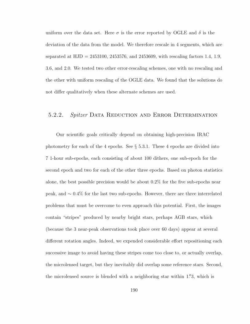
uniform over the data set. Here σ is the error reported by OGLE and δ is the

deviation of the data from the model. We therefore rescale in 4 segments, which are

separated at HJD = 2453100, 2453576, and 2453609, with rescaling factors 1.4, 1.9,

3.6, and 2.0. We tested two other error-rescaling schemes, one with no rescaling and

the other with uniform rescaling of the OGLE data. We found that the solutions do

not differ qualitatively when these alternate schemes are used.

5.2.2. Spitzer Data Reduction and Error Determination

Our scientific goals critically depend on obtaining high-precision IRAC

photometry for each of the 4 epochs. See § 5.3.1. These 4 epochs are divided into

7 1-hour sub-epochs, each consisting of about 100 dithers, one sub-epoch for the

second epoch and two for each of the other three epochs. Based on photon statistics

alone, the best possible precision would be about 0.2% for the five sub-epochs near

peak, and ∼ 0.4% for the last two sub-epochs. However, there are three interrelated

problems that must be overcome to even approach this potential. First, the images

contain “stripes” produced by nearby bright stars, perhaps AGB stars, which

(because the 3 near-peak observations took place over 60 days) appear at several

different rotation angles. Indeed, we expended considerable effort repositioning each

successive image to avoid having these stripes come too close to, or actually overlap,

the microlensed target, but they inevitably did overlap some reference stars. Second,

the microlensed source is blended with a neighboring star within 1.′′3, which is

190

easily resolved in HST images and clearly resolved in OGLE images as well. Third,

this problem is significantly complicated by the well-known fact that IRAC 3.6 µm

images are undersampled.

We apply the procedures of Reach et al. (2005) to perform aperture photometry

on the Basic Calibrated Data (BCD), which includes array-location-dependent and

“pixel-phase” photometric corrections at the few percent level. We choose 7 bright

and isolated stars, which we select from the OGLE images. The HST frames are

of course even better resolved, but they are too small to contain a big enough

sample of reference stars. The centroid position of the target-star aperture on each

of the (roughly 100) BCD dithers is determined by aligning the comparison stars

with the OGLE coordinates. We determine the “internal error” for the target star

and the comparison stars at each sub-epoch from the internal scatters in their

measurements. This is typically very close to the photon limit. However, we find

that the epoch-to-epoch scatter in the comparison stars is about 0.7%. While in

principle this could be due to intrinsic variability, such variability is unlikely to be

so pervasive at this level, particularly since any star showing variability in the I

band over several years was excluded as a reference star. Hence, we attribute this

variation to unknown epoch-to-epoch systematics, and we assume that these affect

the target in the same way that they affect the reference stars. Hence, we adopt

0.7% as our photometric error for each of the 7 Spitzer sub-epochs.

191

We also attempted to do point-spread-function (rather than aperture)

photometry, making use of “Point Response Functions” available at the Spitzer

Science Center Web site. However, we found that the reference stars showed greater

scatter between sub-epochs with this approach and so adopted the results from

aperture photometry.

5.3. Complications Alter Strategy and Analysis

Figure 5.1 shows the ground-based light curve with a fit to a standard

(Paczynski 1986) model. The residuals are severe. The model does not include

parallax. However, models that include parallax are quite similar. In the period

before the peak, we were constantly refitting the light curve with every new night’s

data in order to be able to predict the time of peak and thus the time of the second

ToO observation (which was supposed to be symmetric around the peak with the

first). It became increasingly clear that the event was not standard microlensing,

and we began to consider alternate possibilities, including binary source (also called

“xallarap”), binary lens, and variable source. The last was especially alarming

because if the variability were irregular, it would be almost impossible to model at

the high precision required to carry out this experiment, particularly because the

source might vary differently at I and L. Our concern about xallarap led us to

obtain radial-velocity measurements at several epochs near the peak. These turned

192

out to be the same within less than 1 km s−1, which ruled out xallarap for all but

the most pathologically face-on orbits. But regardless of the nature of the anomaly,

it could potentially cause serious problems because much more and better data are

required to accurately model complicated light curves compared to simple ones.

Hence, as described in § 5.2, recognition of the anomaly caused us to significantly

intensify our ground-based observations. Moreover, it also caused us to think more

carefully about how we would extract parallax information from a more complicated

light curve, and this led us to recognize a complication that affects even light curves

that do not suffer from additional anomalies.

5.3.1. Need for Additional Spitzer Observation

Recall that πE,τ is derived from the different peak time t0 as seen from Earth

and Spitzer: if the two Spitzer observations are timed so that the fluxes seen at

Earth are equal to each other (one on the rising and one on the falling wing of the

light curve), then the Spitzer fluxes will nevertheless be different, the first one being

higher if the event peaks at Spitzer before the Earth. However, the two Spitzer fluxes

may differ not only because Spitzer is displaced from the Earth along the direction

of lens-source relative motion, but also if it is displaced in the orthogonal direction

by different amounts at the two epochs. Gould (1999) recognized this possibility,

but argued that the amplitude of this displacement could be determined from the

measurement of πE,‖, which is derived from the ground-based parallax measurement

193

(i.e., from the asymmetry of the light curve). Hence, he argued that it would be

possible to correct for this additional offset and still obtain a good measurement of

πE,τ . Unfortunately, while it is true that the amplitude can be so derived, the sign of

this correction is more difficult to determine.

The problem can be understood by considering the work of Smith et al. (2003),

who showed that ground-based microlensing parallaxes are subject to a two-fold

degeneracy, essentially whether the source passes the lens on the same or opposite

side of the Earth compared to the Sun. Within the geocentric formalism of Gould

(2004), this amounts to switching the sign of the impact parameter u0 (which

by convention is normally positive) and leaving all other parameters essentially

unchanged. Smith et al. (2003) derived this degeneracy under the assumption that

the Earth accelerates uniformly during the course of the event. This is a reasonable

approximation for short events, but is grossly incorrect for OGLE-2005-SMC-001,

with its timescale of tE ∼ 0.5 yr. Nevertheless, this degeneracy can hold remarkably

well even for relatively long events, particularly for |u0| ≪ 1. The sign of the

correction to πE,τ depends essentially on whether the absolute value of the impact

parameter as seen from Spitzer is higher or lower than that seen from Earth. While

the algebraic displacement of Spitzer along this direction can be predicted from the

ground-based measurement of the parallax asymmetry (just as Gould 1999 argued),

its effect on the absolute value of u0 depends on whether u0 is positive or negative.

194

If the parallax is sufficiently large, then the ground-based light curve alone can

determine the sign of u0, and if it is sufficiently small, the difference between the two

solutions is also very small and may not be significant. However, for intermediate

values of the parallax, this degeneracy can be important. To understand how

an additional Spitzer observation can help, consider an idealized set of four

observations, one at peak, one at baseline, and two symmetrically timed around

peak (as seen from Earth). Call these fluxes fP , fb, f−, and f+. Consider now

the ratio [fP − fb]/[(f− + f+)/2 − fb]. If the impact parameter seen from Spitzer

is higher than that from Earth, this ratio will be lower for the Spitzer data than

for the ground-based data. (Note that blended light, which may be different for

the two sets of observations, cancels out of this expression.) In practice, we found

from simulations that it was not necessary to have the three observations timed

so perfectly. Hence, it was possible to plan both the additional DDT observation,

as well as the second ToO observation to occur during regularly scheduled IRAC

campaigns, so there was no 6.5 hour penalty for either observation. Hence, the net

cost to Spitzer time was less than would have been the case for a single precisely

timed ToO observation.

In brief, the above considerations demonstrate that the Gould (1999) technique

requires a total of four observations, not three as originally proposed. Moreover,

these observations do not have to be so precisely timed as Gould (1999) originally

imagined. See Figure 5.2 for a visual explanation of these arguments.

195

5.3.2. Eight-fold Way

Ultimately, we found that the anomaly was caused by a binary lens. Binary

lenses are subject to their own discrete degeneracies. This means that analysis of

the event is impacted by two distinct classes of discrete degeneracies: those due to

parallax and thoese due to binarity. The discrete parallax degeneracy, as summarized

in § 5.3.1, takes the impact parameter u0 → −u0 and (because u0 ≪ 1) leaves other

parameters changed by very little (see Gould 2004).

The discrete binary degeneracy is between wide and close binaries. Here “wide”

means b ≫ 1 and “close” means b ≪ 1, where b is the angular separation between the

two binary components in units of θE, (for which we give and justify our convention

in § 5.4.1). It gives (bc, qc) → (bw, qw),

bw =1 + qc

1 − qc

b−1c , qw =

qc

(1 − qc)2(5.3)

and leaves other parameters roughly unchanged. Here q is the mass ratio of the lens,

with the convention that for qw, the component closer to the source trajectory goes

in the denominator of the ratio. In both cases, the central magnification pattern is

dominated by a 4-cusp caustic.

This degeneracy was first discovered empirically by Albrow et al. (1999b) and

theoretically by Dominik (1999b) and can be incredibly severe despite the fact that

196

the two caustics are far from identical: the solutions can remain indistinguishable

even when there are two well-observed caustic crossings (An 2005).

In the present case, the deviations from a simple lens are not caused by caustic

crossings, but rather by a close approach to a cusp, which makes this degeneracy

even more severe. In fact, the caustic is symmetric enough that the approach may

almost equally well be to either of two adjacent cusps. That is, the cusp degeneracy

would be “perfect” if the cusp were four-fold symmetric, and it is only the deviation

from this symmetry that leads to distinct solutions for different cusp approaches.

In brief, the lens geometry is subject to an 8-fold discrete degeneracy, 2-fold for

parallax, 2-fold for wide/close binary, and 2-fold for different cusp approaches.

5.4. Binary Orbital Motion

Of course all binaries are in Kepler orbits, but it is usually possible to ignore

this motion in binary-lens analyses. Stated less positively, it is rarely possible to

constrain any binary orbital parameters from microlensing light curves. In the few

known exceptions, (Albrow et al. 2000a; An et al. 2002), the light curve contained

several well-measured caustic crossings that pinned down key times in the trajectory

to O(10−5) of an Einstein crossing time. Hence, we did not expect to measure binary

rotation in the present case in which there are no such crossings.

197

We were nevertheless led to investigate rotation by the following circumstance.

When we initially analyzed the event using only ground-based data, we found that

the best fit (for all 8 discrete solutions) had negative blended light, roughly −10%

of the source light, but with large errors and thus consistent with zero at the 1.5 σ

level. This was not unexpected. As mentioned in § 5.1, the component of the

microlens parallax perpendicular to the Sun, πE,⊥, is generally poorly constrained

by ground-based data alone. The reason for this is that small changes in πE,⊥, the

Einstein timescale tE, the impact parameter u0, the source flux fs, and the blended

flux, fb, all induce distortions in the light curve that are symmetric about the

peak, and hence all these parameters are correlated. Thus, the large errors (and

consequent possible negative values) of fb are just the obverse of the large errors in

πE,⊥. Indeed, this is the reason for adding in Spitzer observations.

However, we found that when the Spitzer observations were added, the blending

errors were indeed reduced, but the actual value of the blending remained highly

negative, near −10%. This prompted us to look for other physical effects that could

induce distortions in the light curve that might masquerade as negative blending.

First among these was binary orbital motion. Before discussing this motion, we first

review microlensing by static binaries.

198

5.4.1. Static Binary Lens Parameters

Point-lens microlensing is described by three geometric parameters, the impact

parameter u0 (smallest lens-source angular separation in units of θE), the time

at which the separation reaches this minimum t0, and the Einstein crossing time

tE = θE/µ, where µ is the lens-source relative proper motion.

In binary lensing, there are three additional parameters, the projected

separation of the components (in units of θE) b, the mass ratio of the components q,

and the angle of the source-lens trajectory relative to the binary axis, φ. Moreover

the first three parameters now require more precise definition because there is no

longer a natural center to the system. One must therefore specify where the center

of the system is. Then u0 becomes the closest approach to this center and t0 the

time of this closest approach. Finally, tE is usually taken to be the time required to

cross the Einstein radius defined by the combined mass of the two components.

In fact, while computer programs generally adopt some fairly arbitrary point

(such as the midpoint between the binaries or the binary center of mass), the

symmetries of individual events can make other choices much more convenient. That

is certainly the case here. Moreover, symmetry considerations that are outlined

below will also lead us to adopt a somewhat non-standard tE for the wide-binary

case, namely the timescale associated with the mass that is closer to the source

trajectory, rather than the total mass. To be consistent with this choice, we also

199

express b as the separation between wide components in units of the Einstein radius

associated with the nearest mass (rather than the total mass).

As is clear from Figure 5.1, the light curve is only a slightly perturbed version

of standard (point-lens) microlensing, which means that it is generated either by the

source passing just outside the central caustic of a close binary (that surrounds both

components) or just outside one of the two caustics of a wide binary (each associated

with one component). In either case, the standard point-lens parameters u0 and t0

will be most closely reproduced if the lens center is placed at the so-called “center

of magnification”. For close binaries this lies at the binary center of mass. For wide

binaries, it lies q(1 + q)−1/2b−1 from the component that is closer to the trajectory.

Hence, it is separated by approximately bq/(1 + q) from the center of mass. This will

be important in deriving equation (5.4), below.

For light curves passing close to the diamond caustic of a close binary, the

standard Einstein timescale (corresponding to the total mass) will be very close to

the timescale derived from the best-fit point lens of the same total mass. However,

for wide binaries, the standard Einstein timescale is longer by a factor (1 + q)1/2,

where q is the ratio of companion (whether heavier or lighter) to the component that

is approached most closely. This is because the magnification is basically due just

to this latter component (with the companion contributing only minor deviations

via its shear), while the usual Einstein radius is based on the total mass. For wide

200

binaries, we therefore adopt an Einstein radius and Einstein timescale reduced by

this same factor.

The advantage of adopting these parameter definitions is that, being fairly well

fixed by the empirical light curve, they are only weakly correlated with various other

parameters, some of which are relatively poorly determined.

5.4.2. Binary Orbital Parameters

While close and wide binaries can be (and in the present case are) almost

perfectly degenerate in the static case, binary orbital motion has a radically different

effect on their respective light curves. Note first that while 7 parameters would be

required to fully describe the binary orbital motion, even in the best of cases it has

not proven possible to constrain more than 4 of them (Albrow et al. 2000a; An et al.

2002). Two of these have already been mentioned, i.e., b and q, from the static case.

For the two binaries for which additional parameters have been measured, these have

been taken to be a uniform rotation rate ω and a uniform binary-expansion rate b.

This choice is appropriate for close binaries because for these, the center of

mass is the same as the center of magnification. Hence the primary effects of binary

motion are rotation of the magnification pattern around the center of magnification

and the change of the magnification pattern due to changing separation. Both

201

of these changes may be (probably are) nonuniform, but as the light curves are

insensitive to such subtleties, the simplest approximation is uniform motion.

However, the situation is substantially more complicated for wide binaries,

consideration of which leads to a different parameterization. Recall that the

wide-binary center of magnification is not at the center of mass, and indeed is close

to one of the components. Hence, as the binary rotates, the center of magnification

rotates basically with that component. Nominally, the biggest effect of this rotation

is the resulting roughly linear motion of the lens center of magnification relative to

the source. However, the linear component of this motion, i.e., the first derivative of

the motion at the peak of the event, is already subsumed in the source-lens relative

motion in the static-binary fit. The first new piece of information about the binary

orbital motion is the second derivative of this motion, i.e., the acceleration. Note

that the direction of this acceleration is known: it is along the binary axis. Moreover,

for wide binaries, Kepler’s Third Law predicts that the periods will typically be

much longer than the Einstein timescale, so to a reasonable approximation, this

direction remains constant during the event. We designate the acceleration (in

Einstein radii per unit time squared) as αb.

The parameter αb is related to the distance to the lens in a relatively

straightforward way. For simplicity, assume for the moment that the center of

magnification is right at the position of the component that is closer to the source

trajectory (instead of just near it). The 3-dimensional acceleration of the component

202

is a = GM2/(brE csc i)2, where M2 is the mass of the companion to the closer

component, rE is the physical Einstein radius, and i is the angle between the binary

axis and the line of sight. Hence, αb = a sin i/rE = (q/b2)GM1 sin3 i/r3E, where M1

is the mass of the closer component. This can be simplified with the aid of the

following three identities: 1) 4GM1/c2 = rEθE, 2) rE = DLθE, 3) rE/rE = DLS/DS.

Here DL and DS are the distances to the lens and source, and DLS = DS − DL. We

then find,

αb

πE

=γc2 sin3 i

4DLAU

D2S

D2LS

, (5.4)

where γ ≡ q/b2 is the shear. Note that the shear determines the size of the caustic

and so is one of the parameters that is most robustly determined from the light curve.

If we were to take account of the offset between M1 and the center of magnification,

the r.h.s. of equation (5.4) would change fractionally by the order of b−2.

5.4.3. Summary of Parameters

Thus, the model requires a total of 10 geometrical parameters in addition

to the 8 flux parameters (fs and fb for each of the 3 ground-based observatories

plus Spitzer). These are the three standard microlensing parameters, t0, u0, tE

(the time of closest approach, separation at closest approach in units of θE, and

Einstein timescale), the three additional static-binary parameters b, q, φ (the binary

separation in units of θE, the binary mass ratio, and the angle of the source trajectory

203

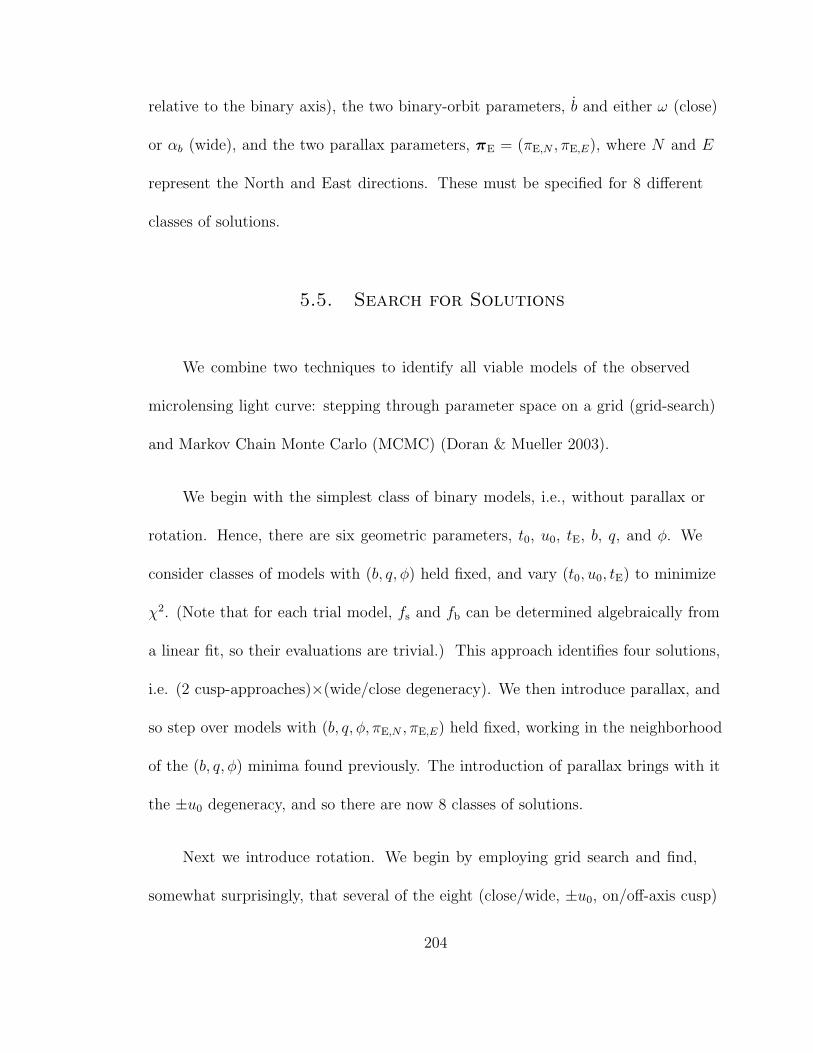
relative to the binary axis), the two binary-orbit parameters, b and either ω (close)

or αb (wide), and the two parallax parameters, πE = (πE,N , πE,E), where N and E

represent the North and East directions. These must be specified for 8 different

classes of solutions.

5.5. Search for Solutions

We combine two techniques to identify all viable models of the observed

microlensing light curve: stepping through parameter space on a grid (grid-search)

and Markov Chain Monte Carlo (MCMC) (Doran & Mueller 2003).

We begin with the simplest class of binary models, i.e., without parallax or

rotation. Hence, there are six geometric parameters, t0, u0, tE, b, q, and φ. We

consider classes of models with (b, q, φ) held fixed, and vary (t0, u0, tE) to minimize

χ2. (Note that for each trial model, fs and fb can be determined algebraically from

a linear fit, so their evaluations are trivial.) This approach identifies four solutions,

i.e. (2 cusp-approaches)×(wide/close degeneracy). We then introduce parallax, and

so step over models with (b, q, φ, πE,N , πE,E) held fixed, working in the neighborhood

of the (b, q, φ) minima found previously. The introduction of parallax brings with it

the ±u0 degeneracy, and so there are now 8 classes of solutions.

Next we introduce rotation. We begin by employing grid search and find,

somewhat surprisingly, that several of the eight (close/wide, ±u0, on/off-axis cusp)

204

classes of solutions have more than one minimum in (ω, b) for close binaries or (αb, b)

for wide binaries. We then use each of these solutions as seeds for MCMC and find

several additional minima that were too close to other minima to show up in the

grid search. Altogether there are 20 separate minima, 12 for close binaries and 8 for

wide binaries.

We use MCMC to localize our solutions accurate to about 1σ and to determine

the covariance matrix of the parameters. In MCMC, one moves randomly from one

point in parameter space to another. If the χ2 is lower, the new point is added to

the “chain”. If not, one draws a random number and adds the new point only if

this number is lower than relative probability (exp(−∆χ2/2)). If the parameters

are highly correlated (as they are in microlensing) and the random trial points are

chosen without reference (or without proper reference) to these covariances, then the

overwhelming majority of trial points are rejected. We therefore sample parameter

space based on the covariance matrix drawn from the previous “links” in the chain.

During the initial ”burning in” stage of the MCMC, we frequently evaluate the

covariance matrix (every 100 “links”) until it stabilizes. Then we hold the covariance

matrix fixed in the simulation (Doran & Mueller 2003). From the standpoint of

finding the best χ2, one can combine linear fits for the flux parameters fs and fb with

MCMC for the remaining parameters. However, since part of our MCMC objective

is to find the covariances, we treat (fs, fb)OGLE as MCMC parameters while fitting

for the remaining four flux parameters analytically.

205

In order to reduce the correlations among search parameters, we introduce

the following parameter combinations into the search: teff ≡ u0tE, fbase = fs + fb,

fmax ≡ fs/u0, and γ ≡ q/b2 (wide) or Q ≡ b2q/(1 + q)2 (close). Because these are

directly related to features in the light curve, they are less prone to variation than

the naive model parameters. The effective timescale teff is 1/√

12 of the full-width

at half-maximum, fbase is just the flux at baseline, and fmax is the flux at maximum.

The scale of the Chang-Refsdal (1979, 1984) distortion (which governs the binary

perturbation) is given by the shear γ for wide binaries and by the quadrupole Q for

close binaries.

The MCMC “chain” automatically samples points in the neighborhood of the

minimum with probability density proportional to their likelihoods, exp(−χ2/2).

Somewhat paradoxically, this means that for higher-dimensional problems, it does

not actually get very close to the minimum. Specifically, for a chain of length

N sampling an m-dimensional space, there will be only one point for which ∆χ2

(relative to the minimum) obeys ∆χ2 < Y , where P [χ2(m dof) < Y ] = N−1. Hence,

for m ≫ 1 one requires a chain of length N ∼ e1/2(m/2)!2m/2 to reach 1σ above

the true minimum, or N ∼ 104.9 for m = 12. Further improvements scale only

as ∼ N1/m. Hence, to find the true minimum, we construct chains in which the

rejection criterion is calculated based on exp(−25χ2/2) rather than exp(−χ2/2).

However, when calculating error bars and covariances, or when integrating over the

MCMC, we use the exp(−χ2/2) chain.

206

5.5.1. Convergence

A general problem in MCMC fitting is to determine how well the solution

“converges”, that is, how precisely the “best fit” solution is reproduced when the

initial seed solution is changed. In our case, the problem is the opposite: MCMC

clearly does not converge to a single minimum, and the challenge is to find all the

local minima. We described our procedure for meeting this challenge above, first

by identifying 8 distinct regions of parameter space semi-analytically, and then

exploring these with different MCMC seeds. This procedure led to well-defined

minima (albeit a plethora of them), whose individual structures were examined by

putting boundaries into the MCMC code that prevented the chain from “drifting”

into other minima. We halted our subdivision of parameter space when the structure

on the χ2 surface fell to of order ∆χ2 ∼ 1, regarding the ∆χ2 ∼< 1 region as the zone

of convergence. As mentioned above, we located the final minimum by artificially

decreasing the errors by a factor of 5, again making certain that the resulting

(exaggerated) χ2 surface was well behaved.

5.6. Solution Triage

Table 1 gives parameter values and errors for a total of 20 different discrete

solutions, which are labeled by (C/W) for close/wide binary, (+/−) for the sign

of u0, (‖/⊥) for solutions that are approximately parallel or perpendicular to the

207

binary axis, and then by alphabetical sequential for different viable combinations of

rotation parameters. In Table 1, we allow a free fit to blending.

Note that some solutions have severe negative blending. While it is possible in

principle that these are due to systematic errors, the fact that other solutions have

near-zero blending and low χ2 implies that the negative-blending solutions probably

have lens geometries that do not correspond to the actual lens. Other solutions have

relatively high χ2 and so are also unlikely. Solutions with χ2 that is less than 9 above

the minimum have their χ2 displayed in boldface, while the remaining solutions are

shown in normal type.

There are several reasons to believe that the blending is close to zero. First, the

source appears isolated on our K-band NICMOS HST images, implying that if it is

blended, this blended light must be within of order 100 mas of the source. As the

density of sources in the HST images is low, this is a priori very unlikely unless the

blended light comes from a companion to the source or the lens. Moreover, all the

near neighbors of the source on the HST image are separately resolved by the OGLE

photometry, so if there is blended light in the OGLE photometry then it must also

be blended in the HST images. Second, the V − I color of the source, which can be

derived by a model-independent regression of V flux on I flux, is identical within

measurement error to the color of the baseline light from the combined source and

(possible) blend. This implies that either 1) the source is unblended, 2) it is blended

by another star of nearly the same color as the source, or 3) it is blended by a star

208

that is so faint that it hardly contributes to the color of the blend. The second

possibility is strongly circumscribed by the following argument. The source is a

clump star. On the SMC CMD, there are first ascent giants of color similar to the

source from the clump itself down to the subgiant branch about 2.5 mag below the

clump. Thus, in principle, the blended light could lie in the range 0.1 ∼< fb/fs ∼< 1

without causing the baseline color to deviate from the source color. However, there

are no solutions in Table 1 with blending this high. There is one low-χ2 solution

with fb/fs ∼ 0.06, but this would be 3 mag below the clump and so below the

subgiant branch. If we restrict the blend to turnoff colors, i.e., V − I = 0.6, then

the color constraint implies fb/fs = 0.01 ± 0.01, which is negligibly small from our

perspective. Thus, while it is possible in principle that the source is blended with

a reddish subgiant, the low stellar density in the HST image, the low frequency of

such subgiants on the CMD, and the difficulty of matching color constraints even

with such a star, combine to make this a very unlikely possibility. We therefore

conduct the primary analysis assuming zero blending, as listed in Table 2. Again,

the ∆χ2 < 9 solutions are marked in boldface. Note that most solutions in Table

1 are reasonably consistent with zero blending, which is the expected behavior for

the true solution provided it is not corrupted by systematic errors. For these, the χ2

changes only modestly from Table 1 to Table 2. However, several solutions simply

disappear from Table 2. This is because, in some cases, forcing the blending to zero

has the effect of merging two previously distinct binary-rotation minima.

209

The main parameters of interests are πE and the closely related quantity v.

However, for reasons that will be explained below, v can be reliably calculated only

for the close solutions, but not the wide solutions. Hence, we focus first on πE.

Figure 5.3 shows error ellipses for all solutions, color-coded by according to ∆χ2

relative to the global minimum. The right-hand panels show the solutions presented

in Tables 1 and 2, which include the Spitzer data. The left-hand panels exclude these

data. The upper panels are based on a free fit for blending whereas the lower panels

are constrained to zero blending for the OGLE dataset. Comparing the two upper

panels, it is clear that when blending is a fitted parameter, the Spitzer data reduce

the errors in the πE,⊥ direction by about a factor of 3. However, once the blending is

fixed (lower panels), the Spitzer data have only a modest additional effect. This is

expected since πE,⊥ is correlated with blending and one can simultaneously constrain

both parameters either by constraining πE,⊥ with Spitzer data or just by fixing the

blending by hand. Figure 5.4 shows the best overall zero-blending fit to the data.

5.6.1. Wide-Binary Solutions

All eight wide solutions are effectively excluded. When a free fit to blending is

allowed, their χ2 values are already significantly above the minimum. When zero

blending is imposed, only five independent solutions survive and those that have

negative blending are driven still higher. In all five cases to ∆χ2 > 16.

210

5.6.2. Close-Binary Solutions

Eight Of the 11 close solutions survive the imposition of zero blending. Of

these, only one has ∆χ2 < 4, and only another two have ∆χ2 < 8.7 relative to

the best zero-blending solution. We focus primarily on these three, which all have

best-fit parallaxes in the range 0.030 < πE < 0.047 and projected velocities in the

range 210 km s−1 < v < 330 km s−1. These projected velocities are of the order

expected for halo lenses but are about 1 order of magnitude smaller than those

expected for SMC self lensing. Note that because there are multiple solutions, the

errors in v are highly non-Gaussian and are best judged directly from Figures 5.5

and 5.6 (below) rather than quoting a formal error bar.

5.7. Lens Location

When Alcock et al. (1995) made the first measurement of microlensing parallax,

they developed a purely kinematic method of estimating the lens distance (and thus

mass) based on comparison of the measured value of v with the expected kinematic

properties of the underlying lens population. Starting from this same approach,

Assef et al. (2006) devised a test that uses the microlens parallax measurement to

assign relative probabilities to different lens populations (e.g., SMC, Galactic halo,

Galactic disk) based solely on the kinematic characteristics of these populations, and

without making prior assumptions about either the mass function or the density

211

normalization of any population. This is especially useful because, while a plausible

guess can be given for the mass function and normalization of SMC lenses, nothing is

securely known about a putative Galactic halo population. In the present case, the

high projected velocity v immediately rules out Galactic-disk lenses, so we restrict

consideration to the other two possibilities.

We begin by recapitulating the Assef et al. (2006) test in somewhat more

general form. The differential rate of microlensing events of fixed mass M (per

steradian) is

d(6)Γ(M) ≡ d6Γ(M)

d2vL d2vSdDLdDS

= fL(vL)fS(vS)D2SνS(DS)νL(DL)2vrE

D2LS

D2S

, (5.5)

where fL(vL) and fS(vS) are the two-dimensional normalized velocity distributions

of the lenses and sources, νL and νS are the density distributions of the lenses and

sources, v is an implicit function of (DL, DS,vL,vS), and rE is an implicit function

of (DL, DS,M). The method is simply to evaluate the likelihood

L =

∫

d2vL d2vSdDLdDS d(6)Γ(M) exp[−∆χ2(v)/2]∫

d2vL d2vSdDLdDS d(6)Γ(M)(5.6)

for each population separately, and then take the ratio of likelihoods for the two

populations: Lratio ≡ Lhalo/LSMC. Here, ∆χ2(v) is the difference of χ2 relative to

the global minimum that is derived from the microlensing light curve. Note that all

212

dependence on M disappears from L. Equation (5.6) can be simplified in different

ways for each population. In both cases, we express the result in terms of Λ,

Λ ≡ v

v2=

πEtEAU

, (5.7)

rather than v, because it is better behaved in the neighborhood of Λ = 0, just as

trigonometric parallax is better behaved near zero than its inverse, distance.

5.7.1. Halo Lenses

For halo lenses, the depth of the SMC is small compared to DLS and the internal

dispersion of SMC sources is small compared to the bulk motion of the SMC. Hence,

one can essentially drop the three integrations over SMC sources, implying

v =DS

DLS

vL − v⊕ − DL

DLS

vSMC, (5.8)

where vL, v⊕, and vSMC are the velocities of the lens, the “geocentric frame”, and the

SMC (all in the Galactic frame) projected on the plane of the sky. The “geocentric

frame” is the frame of the Earth at the time of the peak of the event. It is the most

convenient frame for analyzing microlensing parallax (Gould 2004) and for this event

is offset from the heliocentric frame by

(v⊙,N, v⊙,E) − (v⊕,N, v⊕,E) = (−24.9,−15.5) km s−1. (5.9)

213

We assume an isotropic Gaussian velocity dispersion for the lenses with

σhalo = vrot/√

2, where vrot = 220 km s−1. After some manipulations (and dropping

constants that would cancel out between the numerator and denominator) we obtain

Lhalo =

∫

exp[−∆χ2(Λ)/2]ghalo(Λ, DL)dDLdΛNorthdΛEast∫

ghalo(Λ, DL)dDLdΛNorthdΛEast

, (5.10)

where

ghalo(Λ, DL) = exp(−v2L/2σ2

halo)νhalo(DL)Λ−5D7/2LS D

1/2L , (5.11)

and where vL is an implicit function of Λ through equations (5.7) and (5.8). We adopt

νhalo(r) = const/(a2halo + r2), where ahalo = 5 kpc and the Galactocentric distance is

R0 = 7.6 kpc. We adopt v⊙ = (10.1, 224, 6.7) km s−1 in Galactic coordinates, which

leads to a 2-dimensional projected velocity of (v⊙,N, v⊙,E) = (126,−126) km s−1

toward the SMC source. From our assumed distances DSMC = 60 kpc and the SMC’s

measured proper motion of (−1.17± 0.18, +1.16± 0.18) (Kallivayalil et al. 2006), we

obtain,

(vSMC,N, vSMC,E) − (v⊙,N, v⊙,E) = (−333, 330) km s−1. (5.12)

214

5.7.2. SMC Lenses

For the SMC, we begin by writing

v =vL/DL − vS/DS

D−1L − D−1

S

= vS +DS

DLS

∆v → vSMC − v⊕ +DSMC

DLS

∆v, (5.13)

where vL and vS are now measured in the geocentric frame and ∆v ≡ vL − vS.

The last step in equation (5.13) is an appropriate approximation because the SMC

velocity dispersion is small compared to its bulk velocity and DLS ≪ DS.

We now assume that the sources and lenses are drawn from the same population,

which implies that the dispersion of ∆v is larger than those of vL and vS by 21/2.

We assume that this is isotropic with Gaussian dispersion σSMC. Again making

the approximation DS → DSMC, we can factor the integrals in equation (5.6) by

evaluating the density integral

η(DLS) =∫

dDLν(DL)ν(DL + DLS), (5.14)

where ν = νL = νS. We then obtain

LSMC =

∫

exp[−∆χ2(Λ)/2]gSMC(Λ, DLS)dDLSdΛNorthdΛEast∫

gSMC(Λ, DLS)dDLSdΛNorthdΛEast

, (5.15)

where

gSMC(Λ, DL) = exp[−(∆v)2/4σ2SMC]η(DLS)D

7/2LS Λ−5, (5.16)

215

and where ∆v is an implicit function of Λ through equations (5.7) and (5.13).

5.7.3. SMC Structure

In order to evaluate equation (5.16) one must estimate σSMC as well as the

SMC density ν along the line of sight, which is required to compute η(DLS). This

requires an investigation of the structure of the SMC.

In sharp contrast to its classic “Magellanic irregular” appearance in blue light,

the SMC is essentially a dwarf elliptical galaxy whose old population is quite regular

in both its density (Zaritsky et al. 2000) and velocity (Harris & Zaritsky 2006)

distributions. Harris & Zaritsky (2006) find that after removing an overall gradient

(more below), the observed radial velocity distribution is well fit by a Gaussian with

σ = 27.5 km s−1, which does not vary significantly over their 4 × 2 (RA,Dec) field.

We adopt the following SMC parameters for the 1-dimensional dispersion

σSMC, the tidal radius rt, and the density profile (along the line of sight),

ν(r) = const/(a2SMC + r2)n/2,

σSMC = 25.5 km s−1, rt = 6.8 kpc, aSMC = 1 kpc, n = 3.3, (5.17)

as we now justify.

The σ = 27.5 km s−1 dispersion reported by Harris & Zaritsky (2006) includes

measurement errors. When the reported errors (typically 10 km s−1 per star) are

216

included in the fit, this is reduced to σSMC = 24.5 km s−1. However, these reported

errors may well be too generous: the statistical errors (provided by D. Zaritsky 2006,

private communication) are typically only 2–3 km s−1, the reported errors being

augmented to account for systematic errors. If the statistical errors are used, we

find σSMC = 26.5 km s−1. D. Zaritsky (2006, private communication) advocates an

intermediate value for this purpose, which leads to σSMC = 25.5 km s−1.

The old stellar population in the SMC is rotating at most very slowly. Harris

& Zaritsky (2006) report a gradient across the SMC of 8.3 km s−1 deg−1, which

they note is a combination of the traverse velocity of the SMC and the solid-body

component of internal bulk motion. As the SMC proper motion was poorly

determined at the time, Harris & Zaritsky (2006) did not attempt to disentangle

these two. However, Kallivayalil et al. (2006) have now measured the SMC proper

motion to be (µN, µE) = (−1.16 ± 0.18, 1.17 ± 0.18) mas yr−1. We refit the Harris

& Zaritsky (2006) data and find ∇vr = (−10.5 ± 1.4, 5.0 ± 0.7) km s−1 deg−1.

Subtracting these two measurements (including errors and covariances) we obtain a

net internal rotation of 5.2 ± 1.6 km s−1 deg−1 with a position angle of 183 ± 30.

Since this rotation is due north-south (within errors), a direction for which the data

have a baseline of only ∼ ±1, and since solid-body rotation is unlikely to extend

much beyond the core, it appears that the amplitude of rotational motion is only

about 5 km s−1, which is very small compared to the dispersion, σSMC. Hence, we

ignore it. In addition, we note that this rotation is misaligned with the HI rotation

217

axis (Stanimirovic et al. 2004) by about 120, so its modest statistical significance

may indicate that it is not real.

As we describe below, our likelihood estimates are fairly sensitive to the tidal

radius rt of the SMC. Proper determination of the tidal radius is a complex problem.

Early studies, made before dark matter was commonly accepted, were carried out for

Kepler potentials and in analogy with stellar and solar-system problems (e.g. King

1962). Read et al. (2006) have calculated tidal radii for a range of potentials and also

for an orbital parameter α that ranges from −1 for retrograde to +1 for prograde.

We choose α = 0 as representative and evaluate their expression for an isothermal

potential and for the satellite being close to pericenter (as is appropriate for the

SMC):

rt

D=

σsat

σhost

(

1 +2 ln ξ

1 − ξ−2

)−1/2

. (5.18)

Here, ξ is the ratio of the apocenter to the pericenter of the satellite orbit, D is the

pericenter distance, and σsat and σhost are the respective halo velocity dispersions.

Because we adopt an n = 3.3 profile, the SMC halo velocity dispersion is larger than

its stellar dispersion by (3.3/2)1/2, implying that σsat/σhost = 3.31/2σSMC/vrot = 0.21.

We adopt ξ = 3 based on typical orbits found by Kallivayalil et al. (2006), which

yields rt = 0.107 DSMC = 6.8 kpc. Note, moreover, that at ξ = 3, d ln rt/d ln ξ ∼ 0.24,

so the tidal radius is not very sensitive to the assumed properties of the orbit.

218

The most critical input to the likelihood calculation is the stellar density along

the line of sight. Of course, images of the SMC give direct information only about

its surface density as a function of position. One important clue to how the two

are related comes from the HI velocity map of Stanimirovic et al. (2004), which

shows an inclined rotating disk with the receding side at a position angle of ∼ 60

(north through east). This is similar to the ∼ 48 position angle of the old-star

optical profile found by Harris & Zaritsky (2006) based on data from Zaritsky et

al. (2000). Hence, the spheroidal old-stellar population is closely aligned to the HI

disk, although (as argued above) the stars in the SMC are pressure- rather than

rotationally-supported. Our best clue to the line-of-sight profile is the major-axis

profile exterior to the position of the source, which lies about 1 kpc to the southwest

of the Galaxy center, roughly along the apparent major axis. The projected surface

density is falling roughly as r−2.3 over the ∼ 1 kpc beyond the source position, from

which we derive a deprojected exponent of n = 3.3. This is similar to the exponent

for Milky Way halo stars. While there is a clear core in the star counts, this may be

affected by crowding, and the core seems to have little impact on the counts beyond

the source position (which is what is relevant to the density profile along the line of

sight). Hence, we adopt aSMC = 1 kpc.

The likelihood ratio is most sensitive to the assumptions made about the

stellar density in the outskirts of the SMC, hence to the power law and tidal radius

adopted. This seems strange at first sight because the densities in these outlying

219

regions are certainly extremely small, whatever their exact values. This apparent

paradox can be understood as follows. For DLS ∼< rt, the leading term in η is

η(DLS) ∼ [D2LS + 4(b2 + a2

SMC)]−n/2, where b = 1.0 kpc is the impact parameter.

In the outskirts, this implies η(DLS) ∼ D−nLS . The integrand in the numerator of

equation (5.15) then scales as exp−[∆v(Λ, DLS)]2/4σ2

SMCD7/2−nLS . For fixed Λ, ∆v

is a rising function of DLS, and so for sufficiently large DLS, the exponential will

eventually cut off the integral. However, for the measured value of Λ (corresponding

to ∆v ≡ |Λ/Λ2 − (vSMC − v⊙)| ∼ 300 km s−1, the cutoff does not occur until

DLS ∼ (2σSMC/v)DSMC ∼ 10 kpc. Thus, as long as the density exponent remains

n ∼< 3.5 and as long as the density is not actually cut off by rt, the integral keeps

growing despite the very low density. On the other hand, a parallel analysis shows

that the denominator in equation (5.15) is quite insensitive to assumptions about

the outer parts of the SMC.

5.7.4. Likelihood Ratios

Using our adopted SMC parameters (eq. [5.17]), we find Lratio ≡ Lhalo/LSMC =

27.4. As discussed in § 5.7.3, this result is most sensitive to the outer SMC density

profile, set by the exponent n and the cutoff rt. If the tidal radius is increased from

rt = 6.8 kpc to rt = 10 kpc and other parameters are held fixed, Lratio = 30.3. If the

exponent is reduced from n = 3.3 to n = 2.7, then Lratio = 29.1. Hence, halo lensing

220

is strongly favored in any case, but by an amount that would vary noticeably if any

of our key model parameters were markedly off.

In carrying out these evaluations, we integrated equations (5.10) and (5.15) over

all solutions with ∆χ2 < 9. These solutions are grouped around three close-binary

minima shown in Table 2. We carried out the integration in two different ways:

over the discrete ensemble of solutions found by the Markov chains and uniformly

over the three error ellipses that were fit to these chains. The results do not differ

significantly. Figures 5.5 and 5.6 show Λ for the Markov-chain solutions superposed

on likelihood contours for SMC and halo lenses respectively.

5.7.5. Kepler Constraints for Close Binaries

Binaries move in Kepler orbits. In principle, if we could measure all the Kepler

parameters then these, together with the measured microlens parallax πE (and

the approximately known source distance DS), would fix the mass and distance to

the lens. While the two orbital parameters that we measure are not sufficient to

determine the lens mass and distance, they do permit us to put constraints on these

quantities.

Consider first the special case of a face-on binary in a circular orbit. Kepler’s

Third Law implies that GM/(brE)3 = ω2 where M is the mass of the lens, b is the

221

binary separation in units of the local Einstein radius rE, and ω is the measured

rotation parameter. Since rE = (DLS/DS)rE, this implies,

c2

4rEb3

D2S

DLD2LS

= ω2 (face − on circular) (5.19)

If one considers other orientations but remains restricted to face-on orbits, then

this equation becomes a (“greater than”) inequality because at fixed projected

separation, the apparent angular speed can only decrease.

Further relaxing to the case of non-circular orbits but with b/b = 0 (i.e., the

event takes place at pericenter), the rhs of equation (5.19) is halved, ω2 → ω2/2,

because escape speed (appropriate for near-parabolic orbits) is√

2 larger than

circular speed. Finally, after some algebra, and again working in the parabolic limit,

one finds that including non-zero radial motion leads to ω2/2 → [ω2 + (b/b)2/4]/2,

and thus to

DLD2LS

D2S

≤ c2

2rEb3

[

ω2 +(b/b)2

4

]−1

. (5.20)

If the rhs of this equation is sufficiently small, then only lenses that are near

the Sun (DL ≪ DS) or near the SMC (DLS ≪ DS) will satisfy it. In practice, we

find that this places no constraint on SMC lenses, but does restrict halo lenses to

be relatively close to the Sun, with the limit varying from ∼ 2 kpc to ∼ 10 kpc

depending on the particular solution being probed and the MCMC realization of

222

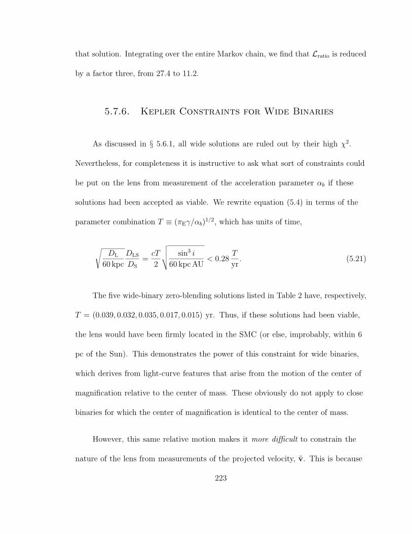
that solution. Integrating over the entire Markov chain, we find that Lratio is reduced

by a factor three, from 27.4 to 11.2.

5.7.6. Kepler Constraints for Wide Binaries

As discussed in § 5.6.1, all wide solutions are ruled out by their high χ2.

Nevertheless, for completeness it is instructive to ask what sort of constraints could

be put on the lens from measurement of the acceleration parameter αb if these

solutions had been accepted as viable. We rewrite equation (5.4) in terms of the

parameter combination T ≡ (πEγ/αb)1/2, which has units of time,

√

DL

60 kpc

DLS

DS

=cT

2

√

√

√

√

sin3 i

60 kpc AU< 0.28

T

yr. (5.21)

The five wide-binary zero-blending solutions listed in Table 2 have, respectively,

T = (0.039, 0.032, 0.035, 0.017, 0.015) yr. Thus, if these solutions had been viable,

the lens would have been firmly located in the SMC (or else, improbably, within 6

pc of the Sun). This demonstrates the power of this constraint for wide binaries,

which derives from light-curve features that arise from the motion of the center of

magnification relative to the center of mass. These obviously do not apply to close

binaries for which the center of magnification is identical to the center of mass.

However, this same relative motion makes it more difficult to constrain the

nature of the lens from measurements of the projected velocity, v. This is because

223

the parallax measurement directly yields only the projected velocity of the center of

magnification, whereas models of the lens populations constrain the motion of the

center of mass. If b is measured, it is straight forward to determine the component

of the difference between these two that is parallel to the binary axis, namely

∆v‖ =b

1 + q

AU

πE

. (5.22)

On the other hand, the measurement of αb indicates that there is motion in the

transverse direction, but specifies neither the amplitude nor sign. For example, for

circular motion with the line of nodes perpendicular to the binary axis,

∆v⊥ = ±√

αbb

1 + q

AU

πE

csc i, (5.23)

and hence,

∆v⊥v

= ±√

αbb

1 + qtE csc i, (5.24)

If this ratio (modulo the csc i term) is small, then the internal motion can be ignored

(assuming the inclination is not unluckily low). In the present case, the quantity

[αbb/(1 + q)]1/2tE for the five respective wide-binary solutions shown in Table 2 is

(0.23,0.36,0.25,1.04,0.77), implying that constraints arising from measurement of v

would be significantly weakened.

Again, however, since the wide solutions are in fact ruled out, all of these

results are of interest only for purposes of illustration.

224

5.7.7. Constraints From (Lack of) Finite-Source Effects

Finite source effects are parameterized by ρ ≡ θ∗/θE, where θ∗ is the angular

size of the source. Equivalently, ρ = (DL/DLS)(r∗/rE), where r∗ = DSθ∗ is the

physical source radius. Since the source is a clump giant, with r∗ ∼ 0.05 AU, this

implies

ρ = 0.021DL

60 kpc

5 kpc

DLS

πE

0.035(5.25)

All models described above assume ρ = 0. Since the impact parameter is u0 ∼ 0.08

and the semi-diameter of the caustic is 2Q ∼ 0.02, finite source effects should be

pronounced for ρ ∼> u0 − 2Q ∼ 0.06. In fact, we find that zero-blending models with

ρ ∼< 0.05 are contraindicated by ∆χ2 ∼ (ρ/0.0196)4. This further militates against

SMC lenses, which predict acceptable values of ρ only for relatively large source-lens

separations. If we penalize solutions with finite source effects by ∆χ2 = (ρ/0.0196)2,

we find that Lratio rises from 11.2 to 20.3.

5.8. Discussion

By combining ground-based and Spitzer data, we have measured the

microlensing parallax accurate to 0.003 units, by far the best parallax measurement

yet for an event seen toward the Magellanic Clouds. Our analysis significantly favors

225

a halo location for the lens over SMC self lensing. It excludes altogether lensing by

Galactic disk stars. Of course, with only one event analyzed using this technique, an

SMC location cannot be absolutely excluded based on the ∼ 5% probability that we

have derived. The technique must be applied to more events before firm conclusions

can be drawn. Spitzer itself could be applied to this task. Even better would be

observations by the Space Interferometry Mission (SIM) (Gould & Salim 1999), for

which time is already allocated for 5 Magellanic Cloud events. SIM would measure

both πE and θE and so determine (rather than statistically constrain) the position

of the lens.

Assuming that the lens is in the halo, what are its likely properties? The mass

is

M = 10.0 M⊙

(

πE

0.047

)−2 πrel

180 µas, (5.26)

where the fiducial πE is the best-fit value and the fiducial πrel is for a “typical”

halo lens, which (after taking account of the constraint developed in § 5.7.5) would

lie at about 5 kpc. In the best-fit model, the mass ratio is q = 2.77, which would

imply primary and secondary masses of 7.3 and 2.7 M⊙ respectively. The projected

separation would be b = 0.22 Einstein radii, i.e., 4.7 AU(DLS/DS). Note that at

these relatively close distances, main-sequence stars in this mass range would shine

far too brightly to be compatible with the strict constraints on blended light. Hence,

the lenses would have to be black holes.

226

We must emphasize that the test carried out here uses only kinematic attributes

of the lens populations and assumes no prior information about their mass functions.

Note, in particular, that if we were to adopt as a priori the lens mass distribution

inferred by the MACHO experiment (Alcock et al. 2000), then the MACHO

hypothesis would be strongly excluded. Recall from § 5.7.5 (eq. [5.20]), that the

lens is either very close to the SMC or within 10 kpc of the Sun. However, from

equation (5.26), for DL < 10 kpc, we have M ∼> 4.6 M⊙, and hence a primary mass

Mq/(1 + q) ∼> 3.4 M⊙. From Figures 12–14 of Alcock et al. (2000), such masses are

strongly excluded as the generators of the microlensing events they observed toward

the LMC.

Hence, if the MACHO hypothesis favored by this single event is correct, the

MACHO population must have substantially different characteristics from those

inferred by Alcock et al. (2000), in particular, as mentioned above, a mass scale of

order 10M⊙ or perhaps more. Alcock et al. (2001b) limit the halo fraction of such

objects to < 30% at M = 10 M⊙ and to < 100% at M = 30 M⊙. At higher masses,

the sensitivity of microlensing surveys deteriorates drastically. However, Yoo et al.

(2004c) derived important limits in this mass range from the distribution of wide

binaries in the stellar halo, putting an upper limit at 100% for M = 40 M⊙ and at

20% for M > 200 M⊙. Thus, if the MACHO hypothesis is ultimately confirmed,

this would be a new population in the mass “window” identified in Figure 7 of Yoo

et al. (2004c) between the limits set by microlensing and wide-binary surveys. This

227

again argues for the importance of obtaining space-based parallaxes on additional

microlensing events.

As we discussed in some detail in § 5.7.3 (particularly the last paragraph) our

conclusion regarding the relatively low probability of the lens being in the SMC

rests critically on the assumption that the SMC lens population falls off relatively

rapidly along the line of sight. (We adopted an n = 3.3 power law.) This is because

equation (5.16) scales ∝ D7/2−nLS . If the SMC had a halo lens population with a

much shallower falloff than we have assumed, this term could dominate the integral

in equation (5.15) even if the overall normalization of the halo were relatively low.

Hence, Magellanic Cloud halo lensing could provide an alternate explanation both

for this SMC event and the events seen by MACHO toward the LMC (Calchi

Novati et al. 2006). As mentioned above, SIM could easily distinguish between this

conjecture and the halo-lens hypothesis.

Finally, we remark that analysis of this event was extraordinarily difficult

because it was a “weak” (i.e., non-caustic-crossing) binary. If it had been either

a single-mass lens or a caustic-crossing binary, it would have been much easier to

analyze and the inferences regarding its location (in the halo or the SMC) would

have been much more transparent. We therefore look forward to applying this same

technique to more typical events.

228

Model t0 u0 tE q Q : γ φ πE,N πE,E ω : α1/2b b/b Fb/Fbase

χ2 (day) (×100) (day) (×100) (deg) (yr−1) (yr−1)

C-‖a 3593.751 −8.729 174.17 2.77 0.980 21.70 −0.0342 0.0319 0.073 5.60 0.003

1455.40 0.040 0.532 8.13 0.33 0.066 1.10 0.0076 0.0047 0.047 0.46 0.061

C+‖a 3593.687 7.763 190.03 2.15 0.850 19.34 −0.0120 0.0236 −0.141 5.83 0.115

1475.74 0.033 0.351 6.58 0.26 0.046 1.26 0.0039 0.0035 0.027 0.48 0.040

C-‖b 3593.560 −9.567 160.61 0.98 0.999 9.23 −0.0069 0.0298 0.331 0.40 −0.101

1462.89 0.036 0.509 6.69 0.25 0.063 1.89 0.0068 0.0049 0.032 0.61 0.060

C+‖b 3593.643 9.321 163.41 1.11 1.002 11.24 −0.0068 0.0199 −0.167 1.33 −0.071

1466.84 0.040 0.346 4.52 0.15 0.046 1.12 0.0036 0.0032 0.029 0.26 0.040

(cont’d)

Table 5.1. OGLE-2005-SMC-001 Light Curve Models: Free Blending.

229

Table 5.1—Continued

Model t0 u0 tE q Q : γ φ πE,N πE,E ω : α1/2b b/b Fb/Fbase

χ2 (day) (×100) (day) (×100) (deg) (yr−1) (yr−1)

C-‖c 3593.473 −9.020 171.06 0.29 0.837 −3.34 0.0070 0.0069 0.746 −3.87 −0.030

1463.52 0.042 0.352 5.89 0.04 0.041 1.31 0.0051 0.0039 0.069 0.44 0.043

C+‖c 3593.460 9.207 167.46 0.29 0.853 −3.78 0.0038 0.0029 −0.743 −3.92 −0.053

1465.15 0.042 0.276 4.15 0.03 0.035 1.24 0.0032 0.0031 0.070 0.41 0.033

C-‖d 3593.639 −9.831 157.29 0.90 1.052 8.53 −0.0121 0.0166 0.146 −0.04 −0.131

1464.13 0.058 0.480 6.18 0.15 0.062 1.18 0.0067 0.0062 0.096 0.27 0.057

C+‖d 3593.676 9.406 162.74 0.79 1.001 7.86 −0.0042 0.0135 −0.144 −0.12 −0.080

1467.70 0.056 0.333 4.42 0.14 0.043 1.47 0.0036 0.0043 0.048 0.50 0.040

(cont’d)

230

Table 5.1—Continued

Model t0 u0 tE q Q : γ φ πE,N πE,E ω : α1/2b b/b Fb/Fbase

χ2 (day) (×100) (day) (×100) (deg) (yr−1) (yr−1)

C+‖e 3593.655 9.161 165.60 1.10 0.983 11.36 −0.0055 0.0197 −0.162 1.50 −0.051

1474.32 0.047 0.498 7.24 0.20 0.060 1.42 0.0038 0.0045 0.038 0.74 0.058

C+‖f 3593.769 7.516 194.33 1.86 0.826 19.21 −0.0078 0.0170 −0.018 5.94 0.140

1474.40 0.038 0.372 7.10 0.33 0.048 1.46 0.0042 0.0038 0.041 0.72 0.042

C-⊥a 3593.251 −8.026 176.25 1.74 0.719 280.21 −0.0101 0.0309 0.758 1.10 0.061

1457.55 0.030 0.370 6.94 0.20 0.041 0.53 0.0054 0.0043 0.049 0.34 0.046

C+⊥a 3593.272 7.900 177.32 1.40 0.752 280.03 −0.0079 0.0198 −0.599 1.45 0.073

1470.74 0.035 0.298 5.33 0.25 0.052 0.58 0.0035 0.0038 0.084 0.32 0.037

(cont’d)

231

Table 5.1—Continued

Model t0 u0 tE q Q : γ φ πE,N πE,E ω : α1/2b b/b Fb/Fbase

χ2 (day) (×100) (day) (×100) (deg) (yr−1) (yr−1)

W-‖a 3593.708 −8.470 170.22 2.49 0.936 6.38 0.0073 0.0041 0.241 0.49 −0.004

1471.32 0.037 0.306 5.70 0.40 0.036 0.51 0.0056 0.0033 0.175 0.02 0.038

W+‖a 3593.703 8.568 167.72 2.48 0.950 6.37 0.0050 0.0017 0.273 0.49 −0.016

1471.29 0.035 0.273 4.70 0.40 0.034 0.49 0.0033 0.0029 0.174 0.02 0.033

W-⊥a 3593.562 −8.666 174.41 2.28 1.154 279.74 −0.0039 0.0180 0.841 −0.75 0.009

1474.79 0.067 0.361 6.31 1.03 0.048 0.61 0.0057 0.0054 0.385 0.06 0.043

W+⊥a 3593.641 9.281 165.12 7.39 1.158 279.74 −0.0036 0.0148 0.804 −0.23 −0.060

1480.79 0.062 0.293 4.04 5.71 0.048 0.60 0.0036 0.0042 0.339 0.18 0.034

(cont’d)

232

Table 5.1—Continued

Model t0 u0 tE q Q : γ φ πE,N πE,E ω : α1/2b b/b Fb/Fbase

χ2 (day) (×100) (day) (×100) (deg) (yr−1) (yr−1)

W-⊥b 3593.570 −9.209 166.04 3.21 1.207 279.24 −0.0074 0.0204 0.909 −0.16 −0.054

1475.50 0.062 0.385 5.83 1.92 0.053 0.58 0.0056 0.0051 0.360 0.18 0.046

W+⊥b 3593.659 8.897 171.08 5.28 1.125 280.32 −0.0023 0.0112 0.826 −0.77 −0.016

1480.16 0.068 0.255 3.89 3.53 0.042 0.61 0.0035 0.0046 0.305 0.06 0.030

W-⊥c 3593.492 −9.443 163.30 2.20 1.291 278.45 −0.0108 0.0195 1.094 0.49 −0.086

1474.90 0.046 0.329 5.24 0.51 0.052 0.48 0.0053 0.0050 0.244 0.05 0.040

W+⊥c 3593.534 9.492 162.68 2.96 1.267 278.50 −0.0050 0.0155 1.054 0.44 −0.091

1486.02 0.049 0.249 3.70 0.69 0.043 0.49 0.0035 0.0051 0.252 0.05 0.030

233

Model t0 u0 tE q Q : γ φ πE,N πE,E ω : α1/2b b/b

χ2 (day) (×100) (day) (×100) (deg) (yr−1) (yr−1)

C-‖a 3593.751 −8.755 173.72 2.77 0.984 21.69 −0.0347 0.0316 0.075 5.59

1455.38 0.039 0.028 0.88 0.32 0.018 1.15 0.0027 0.0048 0.047 0.29

C+‖a 3593.648 8.728 171.75 1.42 0.940 14.45 −0.0063 0.0245 −0.191 3.21

1474.91 0.041 0.025 0.58 0.24 0.019 1.51 0.0037 0.0042 0.039 0.59

C-‖b 3593.612 −8.708 173.51 0.85 0.898 9.17 0.0026 0.0300 0.368 1.04

1463.48 0.028 0.020 0.48 0.18 0.017 1.68 0.0021 0.0046 0.030 0.59

(cont’d)

Table 5.2. OGLE-2005-SMC-001 Light Curve Models: Zero Blending.

234

Table 5.2—Continued

Model t0 u0 tE q Q : γ φ πE,N πE,E ω : α1/2b b/b

χ2 (day) (×100) (day) (×100) (deg) (yr−1) (yr−1)

C+‖b 3593.687 8.711 172.11 0.93 0.924 10.57 −0.0008 0.0180 −0.172 1.39

1469.51 0.034 0.021 0.45 0.11 0.016 1.08 0.0016 0.0030 0.028 0.29

C-‖c 3593.488 −8.769 175.52 0.28 0.813 −3.31 0.0103 0.0074 0.753 −3.89

1464.10 0.038 0.023 0.63 0.03 0.017 1.34 0.0019 0.0039 0.062 0.47

C+‖c 3593.493 8.770 174.27 0.27 0.809 −3.67 0.0084 0.0040 −0.735 −3.88

1467.54 0.038 0.023 0.67 0.03 0.017 1.22 0.0015 0.0030 0.065 0.43

(cont’d)

235

Table 5.2—Continued

Model t0 u0 tE q Q : γ φ πE,N πE,E ω : α1/2b b/b

χ2 (day) (×100) (day) (×100) (deg) (yr−1) (yr−1)

C+‖b 3593.687 8.711 172.11 0.93 0.924 10.57 −0.0008 0.0180 −0.172 1.39

1469.51 0.034 0.021 0.45 0.11 0.016 1.08 0.0016 0.0030 0.028 0.29

C+‖d 3593.751 8.725 172.80 0.65 0.919 7.20 0.0025 0.0115 −0.137 −0.11

1470.98 0.051 0.027 0.50 0.10 0.015 1.47 0.0015 0.0041 0.047 0.55

C-⊥a 3593.233 −8.524 166.86 1.77 0.762 279.76 −0.0168 0.0310 0.746 0.73

1460.01 0.031 0.019 0.49 0.23 0.030 0.48 0.0020 0.0049 0.055 0.25

(cont’d)

236

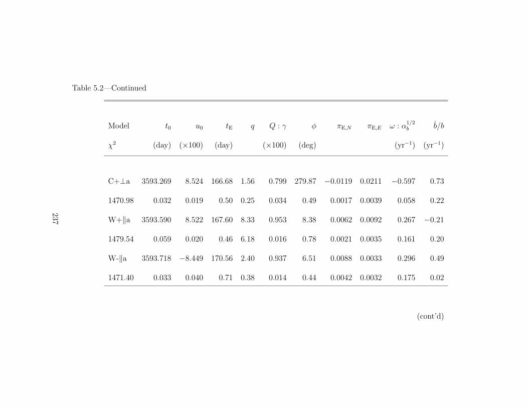
Table 5.2—Continued

Model t0 u0 tE q Q : γ φ πE,N πE,E ω : α1/2b b/b

χ2 (day) (×100) (day) (×100) (deg) (yr−1) (yr−1)

C+⊥a 3593.269 8.524 166.68 1.56 0.799 279.87 −0.0119 0.0211 −0.597 0.73

1470.98 0.032 0.019 0.50 0.25 0.034 0.49 0.0017 0.0039 0.058 0.22

W+‖a 3593.590 8.522 167.60 8.33 0.953 8.38 0.0062 0.0092 0.267 −0.21

1479.54 0.059 0.020 0.46 6.18 0.016 0.78 0.0021 0.0035 0.161 0.20

W-‖a 3593.718 −8.449 170.56 2.40 0.937 6.51 0.0088 0.0033 0.296 0.49

1471.40 0.033 0.040 0.71 0.38 0.014 0.44 0.0042 0.0032 0.175 0.02

(cont’d)

237

Table 5.2—Continued

Model t0 u0 tE q Q : γ φ πE,N πE,E ω : α1/2b b/b

χ2 (day) (×100) (day) (×100) (deg) (yr−1) (yr−1)

W+‖b 3593.709 8.427 170.01 2.41 0.931 6.54 0.0055 0.0021 0.210 0.50

1471.49 0.034 0.037 0.90 0.37 0.014 0.44 0.0030 0.0028 0.163 0.02

W-⊥a 3593.552 −8.742 173.11 2.20 1.169 279.61 −0.0051 0.0179 0.880 −0.73

1474.83 0.067 0.028 1.11 0.97 0.038 0.59 0.0030 0.0055 0.398 0.25

W+⊥a 3593.642 8.759 172.88 4.51 1.115 280.27 −0.0010 0.0126 0.769 −0.76

1480.41 0.069 0.025 1.15 2.76 0.036 0.62 0.0025 0.0051 0.359 0.21

238

OGLE-2005-SMC-001

OGLE I

OGLE V

CTIO I

AUCKLAND

CTIO V

SPITZER

3560 3580 3600 3620 364017

16.5

16

15.5

15

3560 3580 3600 3620 36400.06

0.04

0.02

0

-0.02

-0.04

-0.06

Fig. 5.1.— Standard (Paczynski 1986) microlensing fit to the light curve of OGLE-2005-SMC-001, with data from OGLE I and V in Chile, µFUN I and V in Chile,Auckland clear-filter in New Zealand, and the Spitzer satellite 3.6 µm at ∼ 0.2 AUfrom Earth. The data are binned by the day. All data are photometrically alignedwith the (approximately calibrated) OGLE data. The residuals are severe indicatingthat substantial physical effects are not being modeled. The models do not includeparallax, but when parallax is included, the resulting figure is essentially identical.

239

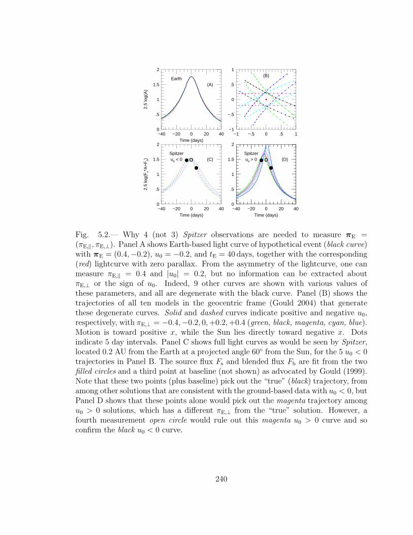
−1 −.5 0 .5 1−1

−.5

0

.5

1(B)

Time (days)2.

5 lo

g(A

)

−40 −20 0 20 400

.5

1

1.5

2

(A)Earth

Time (days)

2.5

log(

Fs*

A+

Fb)

−40 −20 0 20 400

.5

1

1.5

2

(C)Spitzeru0 < 0

Time (days)−40 −20 0 20 400

.5

1

1.5

2

(D)Spitzeru0 > 0

Fig. 5.2.— Why 4 (not 3) Spitzer observations are needed to measure πE =(πE,‖, πE,⊥). Panel A shows Earth-based light curve of hypothetical event (black curve)with πE = (0.4,−0.2), u0 = −0.2, and tE = 40 days, together with the corresponding(red) lightcurve with zero parallax. From the asymmetry of the lightcurve, one canmeasure πE,‖ = 0.4 and |u0| = 0.2, but no information can be extracted aboutπE,⊥ or the sign of u0. Indeed, 9 other curves are shown with various values ofthese parameters, and all are degenerate with the black curve. Panel (B) shows thetrajectories of all ten models in the geocentric frame (Gould 2004) that generatethese degenerate curves. Solid and dashed curves indicate positive and negative u0,respectively, with πE,⊥ = −0.4,−0.2, 0, +0.2, +0.4 (green, black, magenta, cyan, blue).Motion is toward positive x, while the Sun lies directly toward negative x. Dotsindicate 5 day intervals. Panel C shows full light curves as would be seen by Spitzer,located 0.2 AU from the Earth at a projected angle 60 from the Sun, for the 5 u0 < 0trajectories in Panel B. The source flux Fs and blended flux Fb are fit from the twofilled circles and a third point at baseline (not shown) as advocated by Gould (1999).Note that these two points (plus baseline) pick out the “true” (black) trajectory, fromamong other solutions that are consistent with the ground-based data with u0 < 0, butPanel D shows that these points alone would pick out the magenta trajectory amongu0 > 0 solutions, which has a different πE,⊥ from the “true” solution. However, afourth measurement open circle would rule out this magenta u0 > 0 curve and soconfirm the black u0 < 0 curve.

240

Fig. 5.3.— Parallax πE = (πE,N , πE,E) 1 σ error ellipses for all discrete solutions forOGLE-2005-SMC-001. The left-hand panels show fits excluding the Spitzer data,while the right-hand panels include these data. The upper panels show fits withblending as a free parameter whereas the lower panels fix the OGLE blending at zero.The ellipses are coded by ∆χ2 (relative to each global minimum), with ∆χ2 < 1 (red),1 < ∆χ2 < 4 (green), 4 < ∆χ2 < 9 (cyan), 9 < ∆χ2 < 16 (magenta), ∆χ2 > 16(blue). Close- and wide-binary solutions are represented by bold and dashed curves,respectively. Most of the “free-blend, no-Spitzer” solutions are highly degeneratealong the πE,⊥ direction (33 north through east), as predicted from theory, becauseonly the orthogonal (πE,‖) direction is well constrained from ground-based data. Atseen from the two upper panels, the Spitzer observations reduce the errors in the πE,⊥

direction by a factor ∼ 3 when the blending is a free parameter. However, fixing theblending (lower panels) already removes this freedom, so Spitzer observations thenhave only a modest additional effect.

241

OGLE-2005-SMC-001

OGLE I

OGLE V

CTIO I

AUCKLAND

CTIO V

SPITZER

1.5

2

2.5

3

3560 3580 3600 3620 364017

16.5

16

15.5

15

3560 3580 3600 3620 36400.06

0.04

0.02

0

-0.02

-0.04

-0.06

Fig. 5.4.— Best-fit binary microlensing model for OGLE-2005-SMC-001 togetherwith the same data shown in Fig. 5.1. The model includes microlens parallax (twoparameters) and binary rotation (two parameters). The models for ground-basedand Spitzer observations are plotted in blue and red, respectively. All data arein the units of 2.5 log(A), where A is the magnification. Ground-based data arealso photometrically aligned with the (approximately calibrated) OGLE data. Theresiduals show no major systematic trends.

242

6 4 2 0 -2 -4 -6-6

-4

-2

0

2

4

6

Fig. 5.5.— Likelihood contours of the inverse projected velocity Λ ≡ v/v2 for SMClenses together with Λ values for light-curve solutions found by MCMC. The latterare color-coded for solutions with ∆χ2 within 1, 4, and 9 of the global minimum. Thelikelihood contours are spaced by factors of 5.

243

6 4 2 0 -2 -4 -6-6

-4

-2

0

2

4

6

Fig. 5.6.— Likelihood contours of the inverse projected velocity Λ ≡ v/v2 for halolenses together with Λ values for light-curve solutions found by MCMC. Similar toFigure 5.5 except in this case the contours are color coded, with black, red, yellow,green, cyan, blue, magenta, going from highest to lowest.

244

Chapter 6

Probing ∼ 100AU Intergalactic Mg II Absorbing

“Cloudlets” with Quasar Microlensing

6.1. Introduction

Mg II absorbers toward quasar sight lines have been systematically studied since

Lanzetta et al. (1987) (for more recent studies, see Zibetti et al. 2005 and references

therein). Similar Mg II absorbers were subsequently seen in gamma-ray burst (GRB)

spectra. Prochter et al. (2006) compared strong Mg II absorbers toward GRB and

quasar sight lines, and found a significantly higher incidence toward the former.

They proposed three possible effects to explain this discrepancy: (1) obscuration

of faint quasars by dust associated with the absorbers; (2) Mg II absorbers being

intrinsic to GRBs; (3) gravitational lensing of the GRB by the absorbers. However,

they concluded that none of these effects provide a satisfactory explanation.

Frank et al. (2006) proposed a simple geometric solution to this puzzle. They

argued that if Mg II absorption systems are fragmented on scales ∼< 1016cm, similar

to the beam sizes of GRBs, then the observed difference in the frequency of Mg II

245

absorbers would simply reflect the difference in the average beam sizes between

GRBs and quasars, with quasars being several times larger. This explanation

predicts that absorption features due to intervening Mg II cloud fragments should

evolve as the size of GRB afterglow changes, an effect that has now been observed

by Hao et al. (2006). However, the structures of Mg II absorbers down to scales of

∼ 1016cm cannot be directly inferred from their spectral features. Rauch et al. (2002)

put the strongest upper limits on Mg II absorber sizes to date. They observed the

spectra of three images of Q2237+0305 (Huchra et al. 1985) and found that each line

of sight contained individual Mg II absorbers at approximately the same redshift,

but with distinct spectral features. Thus these absorbers are part of a complex that

extends at least ∼ 500pc, but the sizes of the individual “cloudlets” must be smaller

than 200 − 300pc, corresponding to the separations of the macro-images.

Some, if not all, strongly lensed quasars are also gravitationally microlensed

by compact stellar-mass objects in the lensing galaxy (Wambsganss 2006), and

Q2237+0305 was the first lensed quasar found to exhibit significant microlensing

variability (Corrigan et al. 1991; Wozniak et al. 2000). The macro-image of a

microlensed quasar is split into many micro-images, and when the source moves over

the caustic networks induced by the microlenses, those micro-images expand, shrink,

appear, disappear and experience drastic astrometric shifts over timescales of months

or years (Treyer & Wambsganss 2004). The angular sizes of major micro-images are

usually of the same order as those of the quasars, and during the shape and position

246

changes of these images, absorption structures of similar scale along their sight lines

will likely imprint significant variations on the spectrum.

Brewer & Lewis (2005) pioneered the theoretical investigation of quasar

microlensing as a probe of the sub-parsec structure of intergalactic absorption

systems. They concluded that variation in the strength of the absorption lines over

timescales of years or decades caused by microlensing can be used to probe the

structures of Lyman α clouds and associated metal-line absorption systems on scales

∼< 0.1pc. However, as I will show, they significantly underestimated the relevant

timescales for spectral variability given the sizes of the systems they considered.

Thus, they substantially overestimated the scales of absorption structures that

microlensing can effectively probe.

In § 6.2, I lay out the basic theoretical framework of the method. Then in

§ 6.3, I present a numerical simulation of the microlensing of Q2237+0305. I show

that micro-images of this quasar can be used to probe structures of Mg II and other

metal-line absorbing clouds on scales of ∼ 1014 − 1016cm by monitoring the spectral

variations of absorption lines over months or years. Finally in § 6.4, I summarize the

results and discuss their implications.

247

6.2. Varying Microlensed Quasar Image as A “Ruler”

I begin with a brief summary of notation. Subscripts “l”, “s”, “o” and “c”

refer to the lens, source, observer and absorption cloud planes, respectively. The

superscript “ray” is used to refer to the light ray on the cloud plane to distinguish it

from the cloud. The angular diameter distance between object x and y is denoted

Dxy and is always positive regardless of which is closer; in particular, Dx refers to the

angular diameter distance between the observer and object x. The vector angular

position of object x is denoted θx, while its redshift is denoted zx.

Consider an absorbing cloud that is confronted with a “bundle of light rays”

making their way from the source to the lens to the observer. Let rrayc be the position

vector of a point on the plane of the cloud. The line depth 〈Aλ〉 of an absorption

line centered at wavelength λ is given by:

〈Aλ〉 =∫

σλ(rrayc )Aλ(r

rayc )d2rray

c

/∫

σλ(rrayc )d2rray

c (6.1)

where σλ(rrayc ) is the surface density of the “ray bundles” on the plane of the

absorption cloud with the rays weighted by the surface brightness profile of the

quasar and Aλ(rrayc ) is the absorption fraction at rray

c for light of wavelength λ

(Brewer & Lewis 2005).

248

6.2.1. Basic Geometric Configurations and Motions

The absorption cloud can be located either between the lens and observer or

between the lens and source. In the former case, the angular position of the light ray

at the cloud plane is θrayc = θi, so rray

c = θiDc. The projected light rays on the cloud

plane maintain the exact shapes of the quasar images, and their physical extents are

proportional to the distance to the observer.

If the cloud is between the lens and the source, it can be easily shown that θrayc

is given by (Brewer & Lewis 2005):

θrayc =

(

1 − DlcDs

DlsDc

)

θi +DlcDs

DlsDc

θs, (6.2)

so

rrayc =

(

Dc −Dlc

Dls

Ds

)

θi +Dlc

Dls

rs. (6.3)

The lens-source relative proper motion, with time as measured by the observer, is

given (in other notation) by Kayser et al. (1986),

µls =1

1 + zs

vs

Ds

− 1

1 + zl

vl

Dl

+1

1 + zl

voDls

DlDs

(6.4)

where vs, vl, vo are the transverse velocities of the source, lens and observer, relative

to the cosmic microwave background (CMB). In particular,

vo = vCMB − (vCMB · z)z, (6.5)

249

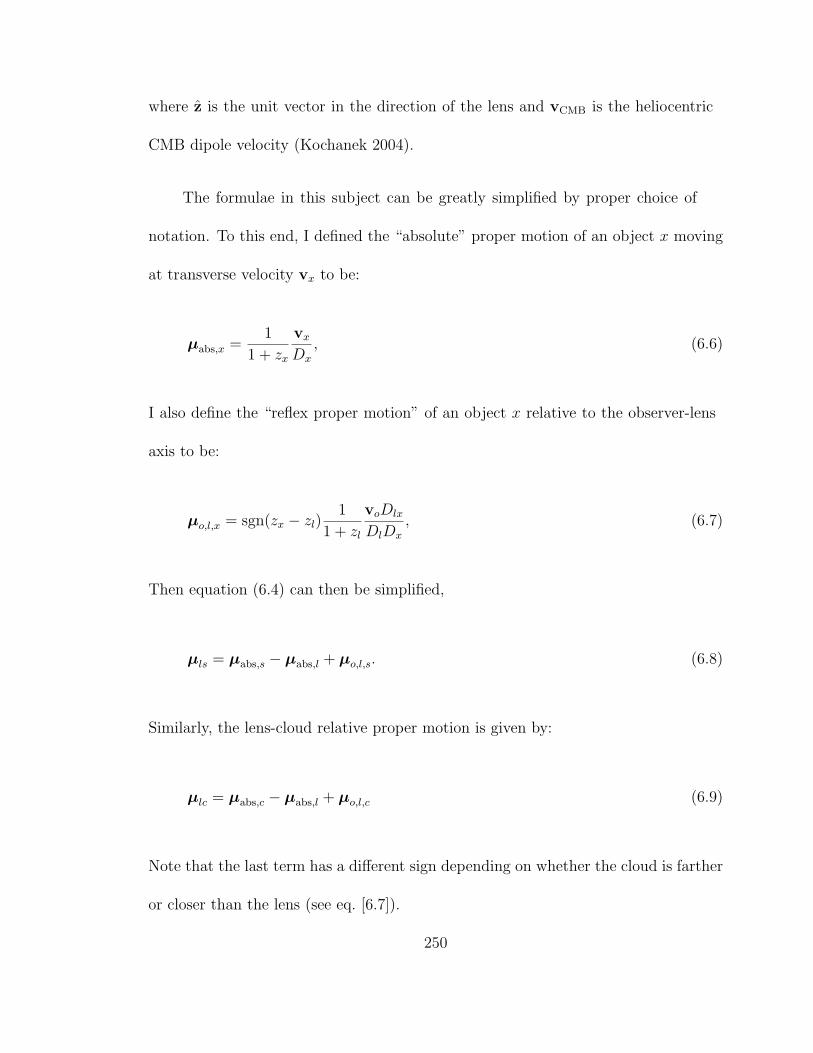
where z is the unit vector in the direction of the lens and vCMB is the heliocentric

CMB dipole velocity (Kochanek 2004).

The formulae in this subject can be greatly simplified by proper choice of

notation. To this end, I defined the “absolute” proper motion of an object x moving

at transverse velocity vx to be:

µabs,x =1

1 + zx

vx

Dx

, (6.6)

I also define the “reflex proper motion” of an object x relative to the observer-lens

axis to be:

µo,l,x = sgn(zx − zl)1

1 + zl

voDlx

DlDx

, (6.7)

Then equation (6.4) can then be simplified,

µls = µabs,s − µabs,l + µo,l,s. (6.8)

Similarly, the lens-cloud relative proper motion is given by:

µlc = µabs,c − µabs,l + µo,l,c (6.9)

Note that the last term has a different sign depending on whether the cloud is farther

or closer than the lens (see eq. [6.7]).

250

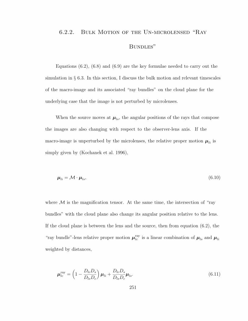
6.2.2. Bulk Motion of the Un-microlensed “Ray

Bundles”

Equations (6.2), (6.8) and (6.9) are the key formulae needed to carry out the

simulation in § 6.3. In this section, I discuss the bulk motion and relevant timescales

of the macro-image and its associated “ray bundles” on the cloud plane for the

underlying case that the image is not perturbed by microlenses.

When the source moves at µls, the angular positions of the rays that compose

the images are also changing with respect to the observer-lens axis. If the

macro-image is unperturbed by the microlenses, the relative proper motion µli is

simply given by (Kochanek et al. 1996),

µli = M · µls, (6.10)

where M is the magnification tensor. At the same time, the intersection of “ray

bundles” with the cloud plane also change its angular position relative to the lens.

If the cloud plane is between the lens and the source, then from equation (6.2), the

“ray bundle”-lens relative proper motion µraylc is a linear combination of µls and µli

weighted by distances,

µraylc =

(

1 − DlcDs

DlsDc

)

µli +DlcDs

DlsDc

µls. (6.11)

251

Substituting equation (6.10) into equation (6.11) yields the bulk proper motion of

the un-microlensed “ray bundle” relative to the lens,

µraylc,bulk =

[(

1 − DlcDs

DlsDc

)

M +DlcDs

DlsDc

I]

· µls. (6.12)

where I is the unit tensor.

When the “ray bundles” are between the source and the lens, their relative bulk

proper motion is simply,

µraylc,bulk = µli = M · µls. (6.13)

There are two major effects that may induce variability of absorption lines

toward a lensed quasar. One is the creation, destruction, distortion and astrometric

shifts of micro-images, which probe structures similar to the size of the micro-images.

The other is the bulk motion of the “ray bundles” relative to the cloud. On the

cloud plane, this motion has an angular speed of ∆µlc,bulk = µraylc,bulk − µlc, and the

time tcc required for the “ray bundles” to cross a cloud of transverse size Rc is,

tcc =Rc

Dc|∆µbulk,lc|=

Rc

Dc|µraybulk,lc − µlc|

. (6.14)

6.3. Application to Q2237+0305

In October 1998, Rauch et al. (2002) obtained high-resolution Keck spectra of

images A, B and C of Q2237+0305. They found Mg II absorption lines at redshifts

252

of z = 0.5656 and z = 0.827 in the spectra of all three images, but absorption profiles

of the individual sight lines differed (e.g., Figs. 6 and 10 of their paper). Therefore,

they concluded that the Mg II complexes giving rise to these absorption features

must be larger than ∼ 0.5kpc, while the individual Mg II components must be

smaller than ∼ 200 − 300h−150 pc. Q2237+0305 is also one of the most observed and

best studied lensed quasars with obvious microlensing features, and the properties

of the system are well known. These factors make it an ideal object to investigate.

The comprehensive statistical study of this lens by Kochanek (2004) showed

that the size of the quasar is ∼ 1015h−1cm − 1016h−1cm. Mortonson et al. (2005)

demonstrated that the source size has a much more significant effect on microlensing

models than the source brightness profile. For simplicity, in the simulation, I model

the source as uniform disks with four different sizes: 1015h−1cm, 3 × 1015h−1cm,

5 × 1015h−1cm and 1016h−1cm. Uniform grids of rays are traced from the image

plane to the source plane (Wambsganss 1990). Because structures of interest have

similar sizes as the source, finite-source effects must be taken into account. The

grid size used has an angular scale 1/10 of the smallest source. Kochanek (2004)

demonstrated that a Salpeter mass function cannot be distinguished from a uniform

mass distribution and found the mean stellar mass to be 〈M 〉 ∼ 0.037h−1M⊙. For

simplicity, I assign all stars in the simulation the same mass of 0.04h−1M⊙. Rays

are shot from a region extending 47〈θE〉 on each side, where 〈θE〉 is the Einstein

radius of a 0.04h−1M⊙ star. I adopt a convergence and shear for image A of

253

(κ, γ) = (0.394, 0.395) from Kochanek (2004), and set the stellar surface density

κ∗ = κ. Four different trajectories, oriented at 0, 30, 60 and 90 degrees with respect

to the direction of the shear are studied. Positions on both the image plane and the

source plane are recorded once a ray falls within a distance of 2 times the largest

source size from any trajectory on the source plane. A total length of 5〈θE〉 along

each trajectory is considered.

Throughout the paper, I adopt a ΛCDM cosmology with Ωm = 0.3, ΩΛ = 0.7

and H0 = 100h km s−1 Mpc−1. The lens and source are at redshifts

zl = 0.0394 and zs = 1.695 (Huchra et al. 1985). These imply (Ds, Dl, Dls) =

(1223, 113, 1180)h−1 Mpc. Based on Kochanek (2004), I adopt transverse velocities

of the lens, source and observer of (vl, vs, vo) = (300, 140, 62)km s−1. The lens

and source absolute proper motions and the source reflex proper motion are

(µabs,l, µabs,s, µo,l,s) = (0.54, 0.009, 0.11) h µas yr−1. So the lens absolute proper

motion dominates the lens-source relative proper motion. It can easily be shown

that the absolute and reflex proper motions of the cloud are much smaller than the

absolute proper motion of the lens unless the cloud redshift is close to or smaller

than the lens redshift. For Q2237+0305, the lens redshift is very small compared

to the source, so most likely zc ≫ zl. Thus, in following analysis, I focus on clouds

with redshift zc > zl, and ignore the absolute and reflex proper motions of the source

254

and the cloud. Under these assumptions, the source and the cloud share the same

relative proper motion,

µlc = µls = −µabs,l (6.15)

In the simulation, as a practical matter, I hold the positions of the observer,

lens galaxy (as well as its microlensing star field) fixed, and allow the source to move

through the source plane at µls. By equation (6.15), the cloud then has the same

relative proper motion as the source. At any given time, the angular positions of

the “ray bundles” are calculated using equation (6.2). Then by simply subtracting

the angular position of the source at that time, the “ray bundles” positions are

transformed to the reference frame of the cloud.

During short timescales, microlensing causes centroid shifts of the macro-image

(Lewis & Ibata 1998; Treyer & Wambsganss 2004) with respect to the steady bulk

motion of “ray bundles” relative to the cloud, which is described in § 6.2.2. If the

direction of relative lens-source proper motion is the same as the lens shear, then by

subtracting µls from equation (6.12), one finds that the “ray bundles” have their

maximum bulk proper motion relative to the cloud,

∆µbulk,lc,max =(

1 − DlcDs

DlsDc

)

(

1

1 − κ − γ− 1

)

µls

∼ 2(

1 − 1.037Dlc

Dc

)

h µas yr−1. (6.16)

255

If the source moves perpendicular relative to the lens shear, ∆µlc =

[1 − DLCDS/(DLSDC)]|1/(1 − κ + γ) − 1|µls, which is approximately 0 for

the (κ, γ) of image A.

Figures 6.1 and 6.2 show the results for a source trajectory that is parallel

to the shear direction. The bottom panel of Figure 6.1 shows the magnification

pattern on the source plane, with a series of 4 concentric circles centered at 5 source

positions; and the top panels show the images at these positions relative to the

source (which has the same proper motion as the cloud). Different colors represent

different source sizes. The middle panel of Figure 6.1 shows the light curves for the

4 source sizes with the blue dashed lines used to mark the times for the five source

positions. Figure 6.2 shows the “ray bundle” positions in the cloud frame at redshifts

1.69, 0.83, 0.57, 0.1. The 5 different columns show the 5 positions corresponding to

those in Figure 6.1.

In the top row of Figure 6.2, one can see that the “ray bundles” at zc = 1.69,

which is very close to the quasar, have almost exactly the same size and shape

as the source and that the bundles show almost no bulk motion. The density of

“ray bundles” clearly have the imprints from the magnification pattern shown in

the bottom panel of Figure 6.1. So if an absorption cloudlet has a size similar to

or somewhat smaller than a source that is sitting directly behind it, the depth of

its corresponding absorption line will change dramatically as the source crosses the

caustics. The magnification close to a fold caustic is proportional to the inverse

256

square root of the distance from it, so for a cloud with angular size θc < θs, the

fractional change in absorption line depth caused by the caustics scales as (θc/θs)3/4.

Hence, for a cloud close to the quasar redshift, structures on scale ∼ 1014−1016h−1cm

(depending on the source size) will be probed over few-month to few-year timescales

(i.e., the timescale of typical caustics crossings).

The fourth row of panels of Figure 6.2 shows “ray bundles” for zc = 0.1, which

is close to the lens redshift. A distinct difference between these “ray bundles”

and the ones at zc = 1.69 is that they are split into many groups of bundles,

which correspond to the micro-images in the top panel of Figure 6.1. I dub these

groups of “ray bundles” as micro-images in the following discussions. Most of these

micro-images are stretched one-dimensionally, and most rays are concentrated in

a few major micro-images. The micro-images in different columns have drastically

different morphologies and positions. If there are cloudlets of similar size as these

micro-images distributed on the cloud plane, then the absorption spectra will show

multi-component absorption features at any given time. These components will

experience drastic changes in line depth, with some components disappearing and

other new components appearing during the course of months or years, as the source

crosses the microlensing caustics. Another important characteristic is that the bulk

of these micro-images are moving in the same direction as the source. This motion

is described by equation (6.16), which yields ∼ 0.8 h µas yr. So from equation (6.14),

structures as large as ∼ 3.0n × 1016 h−1 cm will be crossed in n × 10 h−1 yr by the

257

bulk motion of the “ray bundles”. Hence, the effects caused by the micro-images

and the bulk motion of the bundles together probe scales of ∼ 1014 − 1016h−1cm on

timescales of months to years.

The second and third row of panels in Figure 6.2 refer to clouds at intermediate

redshifts between the lens and the source. Their redshifts, zc = 0.83 and zc = 0.57,

are close to the Mg II absorption systems observed by Rauch et al. (2002). As

expected, the characteristics of these “ray bundles” are intermediate between those

shown in rows 1 and 4. The overall shapes of the micro-images are close to that

of the source, with magnification patterns imprinted on them. And they also

clearly show multiple components, which appear and disappear as the source crosses

caustics. The angular sizes of the images are close to that of the (unmagnified)

quasar. These micro-images could probe clouds with angular size from a factor of

few smaller to a factor of few larger than the source size, which corresponds to scales

of ∼ 1014 − 1016h−1cm. From equation (6.14) and (6.16), the bulk motion of the

bundles will probe cloud structures ∼ 0.8n × 1016 h−1 cm and ∼ 1.3n × 1016 h−1 cm

during n × 10 h−1 yr for zc = 0.83 and zc = 0.57, respectively.

For a source trajectory that is perpendicular to the shear, the “ray bundles”

will exhibit almost no bulk motion relative to the cloud, while the magnitude

of bulk motion for intermediate trajectories is a fraction that is of the parallel

case, depending on the angles of motion relative to the shear direction. And

the micro-images of these trajectories share similar properties with those of the

258

trajectory that is parallel to the shear. Figure 6.2 shows that micro-image motions

are on the same order of magnitude as the bulk motion of the macro-image over the

timescales considered. Therefore, trajectory direction only has a modest impact on

the scales at which cloud can be probed.

These results are contrast significantly with those of Brewer & Lewis (2005),

who claimed that quasar microlensing for image A of Q2237+0305 can induce

considerable variability of absorption lines associated with structures as large as

0.1pc during the course of years to decades. According to their analysis, the effect is

largest when the cloud is very close to the source, and for example, the timescale of

line strength variation for a 0.1pc cloud very close to the source is given as ∼ 16.2yr.

However, in their analysis, they effectively assumed the relative lens-cloud proper

motion µlc = 0. This would lead to a timescale tcc ∼ RcDl/(vlDs) ∼ 16(Rc/0.1pc)yr

for an absorption cloud near the source redshift (they adopted vl = 600km s−1),

which is in agreement with column 4 of their Table 1. In fact, I showed that, when

peculiar velocities of the source and cloud are ignored, µlc = µls (eq. [6.15]), which

is not negligible. Even considering realistic peculiar motions of the source and the

cloud, it still leads to time scales that are more than one order of magnitude slower

than those predicted for µlc = 0. In addition, when the cloud is close to the source,

the angular sizes of the clouds they considered are orders of magnitudes larger than

their source size, so effects of changes in magnification pattern on the source plane

259

alone have very little impact as well. Therefore, Brewer & Lewis (2005) significantly

overestimated the cloud size to which microlensing is effectively sensitive.

6.4. Discussion and Conclusion

I have shown that there are two effects that might induce variation of

absorption lines along the sight lines to lensed quasars. One effect is caused by

the drastic morphological and positional changes of micro-images when the source

crosses the caustic network. The other effect is due to the bulk motion of the

“ray bundles” relative to the absorption clouds. I have laid out a basic framework

in studying these effects for microlensed quasars in general. And in particular, I

performed numerical simulations to apply the method to image A of Q2237+0305.

I demonstrated that the combinations of these two effects probe 1014 − 1016 h−1 cm

absorption cloudlets between the lens and the source over timescales of months to

years. The existence of these cloudlets will be revealed by either changes in line

depths or appearances/disappearances of multi-absorption components. Spectra

should preferably be taken during the course of caustic crossings, which can be

inferred from photometric monitoring programs of lensed quasars. In fact, the Mg II

lines observed by Rauch et al. (2002) about 8 years ago already show different

multi-components along sight lines to three different macro-images, implying they

might be caused by fragmented cloudlets with similar sizes as the micro-images. A

260

similar high-resolution spectrum taken in the near future would provide a definitive

test of the existence for structures of Mg II or other metal-line absorbers at the scales

of 1014 − 1016 h−1 cm. If the spectral variations are indeed observed, a statistical

study similar to Kochanek (2004) will be required to infer the properties of the

cloudlets. Moreover, a time series of spectra may provide additional constraints to

quasar models that are currently based only on photometric-monitoring data.

261

Fig. 6.1.— Caustics network (bottom panel), light curve (middle panel) and imagesrelative to the source position (top panel) for a source trajectory that is parallel to thelens shear (the direction of x-axis). Different colors represent the 4 different sourcesizes.

262

Fig. 6.2.— Physical positions of “ray bundles” in the frame of cloud at redshifts 0.1,0.57, 0.83 and 1.69. The 5 different columns correspond to the source positions shownin Figure 6.1. x-axis is the direction of the lens shear.

263

Appendix A

Two New Finite-Source Algorithms

To model planetary light curves, we develop two new binary-lens finite-source

algorithms. The first algorithm, called “map-making”, is the main work horse. For

a fixed (b, q) geometry, it can successfully evaluate the finite-source magnification of

almost all data points on the light curve and can robustly identify those points for

which it fails. The second algorithm, called “loop-linking”, is much less efficient than

map-making but is entirely robust. We use loop-linking whenever the map-making

routine decides it cannot robustly evaluate the magnification of a point. In addition,

at the present time, map-making does not work for resonant lensing geometries, i.e.,

geometries for which the caustic has six cusps. For planetary mass ratios, resonant

lensing occurs when the planet is very close to the Einstein radius, b ∼ 1. We use

loop-linking in these cases also.

A.1. Map-Making

Map-making has two components: a core function that evaluates the

magnification and a set of auxiliary functions that test whether the measurement

264

is being made accurately. If a light-curve point fails these tests, it is sent to

loop-linking.

Finite-source effects are important when the source passes over or close to

a caustic. Otherwise, the magnification can be evaluated using the point-source

approximation, which is many orders of magnitude faster than finite-source

evaluations. Hence, the main control issue is to ensure that any point that falls

close to a caustic is evaluated using a finite-source algorithm or at least is tested to

determine whether this is necessary. For very high magnification events, the peak

points will always pass close to the central caustic. Hence, the core function of

map-making is to “map” an Einstein-ring annulus in the image plane that covers

essentially all of the possible images of sources that come close to the central caustic.

The method must also take account of the planetary caustic(s), but we address that

problem further below.

We begin by inverse ray-shooting an annulus defined by APSPL > Amin, where

APSPL is the Paczynski (1986) magnification due to a point source by a point lens

and Amin is a suitably chosen threshold. For OGLE-2000-BLG-343, we find that

Amin = 75 covers the caustic-approaching points in essentially all cases. The choice

of the density of the ray-shooting map is described below. Each such “shot” results

in a four-element vector (xi, yi, xs, ys). We divide the portion of the source plane

covered by this map into a rectangular grid with k = 1, . . . , Ng elements. We choose

the size of each element to be equal to the smallest source radius being evaluated by

265

the map. Hence, each “shot” is assigned to some definite grid element k(xs, ys). We

then sort the “shots” by k. For each light-curve point to be evaluated, we first find

the grid elements that overlap the source. We then read sequentially through the

sorted file1 from the beginning of the element’s “shots” to the end. For each “shot”,

we ask whether its (xs, ys) lies within the source. If so, we weight that point by the

limb-darkened profile of the source at that radius. Note that a source with arbitrary

shape and surface brightness profile would be done just as easily.

For each light-curve point, we first determine whether at least one of the images

of the center of the source lies in the annulus. In practice, for our case, the points

satisfying this condition are just those on the night of the peak, but for other events

this would have to be determined on a point-by-point basis. We divide those points

with images outside the annulus into two classes, depending on whether they lie

inside or outside two or three rectangles that we “draw”, one around each caustic.

Each rectangle is larger than the maximum extent of the caustics by a factor of 1.5 in

each direction. If the source center lies outside all of these rectangles, we assume that

the point-source approximation applies and evaluate the magnification accordingly.

If it lies inside one of the rectangles (and so either near or inside one of the caustics),

we perform the following test to see whether the point-source approximation holds.

1Whether this “file” should actually be an external disk file or an array in internal memory

depends on both the size of the available internal memory and the total number of points evaluated

in each lens geometry. In our case, we used internal arrays.

266

We evaluate the point-source magnifications at five positions, namely, the source

center A(0, 0), two positions along the source x-axis A(±λρ∗, 0), and two positions

along the source y-axis A(0,±λρ∗), where λ ≤ 1 is a parameter. We demand that

∣

∣

∣

∣

A(λρ∗, 0) + A(−λρ∗, 0)

2A(0, 0)− 1

∣

∣

∣

∣

+∣

∣

∣

∣

A(0, λρ∗) + A(0,−λρ∗)

2A(0, 0)− 1

∣

∣

∣

∣

< 4σ, (A.1)

where σ is the maximum permitted error (defined in § A.3). We use a minimum of

five values in order to ensure that the magnification pattern interior to the source is

reasonably well sampled; the precise value is chosen empirically and is a compromise

between computing speed and accuracy. We require the number of values to be at

least 2[ρ∗/√

q] in order to ensure that small, well-localized perturbations interior to

the source caused by low mass ratio companions are not missed.

If a point passes this test, the magnification pattern in the neighborhood of the

point is adequately represented by a gradient and so the point-source approximation

holds. Points failing this test are sent to loop linking.

The remaining points, those with at least one image center lying in the annulus,

are almost all evaluated using the sorted grid as described above. However, we must

ensure that the annulus really covers all of the images. We conduct several tests to

this end.

First, we demand that no more than one of the three or five images of the

source center lie outside the annulus. In a binary lens, there is usually one image

267

that is associated with the companion and that is highly demagnified. Hence, it can

generally be ignored, so the fact that it falls outside the annulus does not present a

problem. If more than one image center lies outside the annulus, the point is sent to

loop-linking. Second, it is possible that an image of the center of the source could

lie inside the annulus, but the corresponding image of another point on the source

lies outside. In this case, there would be some intermediate point that lay directly

on the boundary. To guard against this possibility, we mark the “shots” lying within

one grid step of the boundaries of the annulus, and if any of these boundary “shots”

fall in the source, we send the point to loop-linking. Finally, it is possible that

even though the center of the source lies outside the caustic (and so has only three

images), there are other parts of the source that lie inside the caustic and so have

two additional images. If these images lay entirely outside the annulus, the previous

checks would fail. However, of necessity, some of these source points lie directly on

the caustic, and so their images lie directly on the critical curve. Hence, as long as

the critical curve is entirely covered by the annulus, at least some of each of these

two new images will lie inside the annulus and the “boundary test” just mentioned

can robustly determine whether any of these images extend outside the annulus. For

each (b, q) geometry, we directly check whether the annulus covers the critical curve

associated with the central caustic by evaluating the critical curve locus using the

algorithm of Witt (1990).

268

A.2. Loop-Linking

Loop-linking is a hybrid of two methods: inverse ray-shooting and Stokes’s

theorem. In the first method (which was also used above in “map-making”), one

finds the source location corresponding to each point in the image plane. Those

that fall inside the source are counted (and weighted according to the local surface

brightness), while those that land outside the source are not. The main shortcoming

of inverse ray-shooting is that one must ensure that the ensemble of “shots” actually

covers the entire image of the source without covering so much additional “blank

space” that the method becomes computationally unwieldy.

In the Stokes’s theorem approach, one maps the boundary of (a polygon-

approximation of) the source into the image plane, which for a binary lens yields

either three or five closed polygons. These image polygons form the (interior or

exterior) boundaries of one to five images. If one assumes uniform surface brightness,

the ratio of the combined areas of these images (which can be evaluated using

Stokes’s theorem) to the area of the source polygon is the magnification.

There are two principal problems with the Stokes’s theorem approach. First,

sources generally cannot be approximated as having uniform surface brightness.

This problem can be resolved simply by breaking the source into a set of annuli, each

of which is reasonably approximated as having uniform surface brightness. However,

this multiplies the computation time by the number of annuli. Second, there can

269

be numerical problems of several types if the source boundary passes over or close

to a cusp. First, the lens solver, which returns the image positions given the source

position, can simply fail in these regions. This at least has the advantage that one

can recognize that there is a problem and perhaps try some neighboring points. The

second problem is that even though the boundary of the source passes directly over

a cusp, it is possible that none of the vertices of its polygon approximation lie within

the caustic. The polygonal image boundary will then fail to surround the two new

images of the source that arise inside the caustic, so these will not be included in

the area of the image. Various steps can be taken to mitigate this problem, but the

problem is most severe for very low-mass planets (which are of the greatest interest

in the present context), so complete elimination of this problem is really an uphill

battle.

The basic idea of loop-linking is to map a polygon that is slightly larger than

the source onto the image plane, and then to inverse ray shoot the interior regions

of the resulting image-plane polygons. This minimizes the image-plane region

to be shot compared to other inverse-ray shooting techniques. It is, of course,

more time-consuming than the standard Stokes’s theorem technique, but it can

accommodate arbitrary surface-brightness profiles and is more robust. As we detail

below, loop-linking can fail at any of several steps. However, these failures are

always recognizable, and recovery from them is always possible simply by repeating

the procedure with a slightly larger source polygon.

270

Following Gould & Gaucherel (1997), the vertices of the source polygon are

each mapped to an array of three or five image positions, each with an associated

parity. If the lens solver fails to return three or five image positions, the evaluation is

repeated beginning with a larger source polygon. For each successive pair of arrays,

we “link” the closest pair of images that has the same parity and repeat this process

until all images in these two arrays are linked. An exception occurs when one array

has three images and the other has five images, in which case two images are left

unmatched. Repeating this procedure for all successive pairs of arrays produces a set

of linked “strands”, each with either positive or negative parity. The first element of

positive-parity strands and the last element of negative-element strands are labeled

“beginnings” and the others are labeled “ends”. Then the closest “beginning” and

“end” images are linked and this process is repeated until all “beginnings” and

“ends” are exhausted. The result is a set of two to five linked loops. As with the

standard Stokes’s theorem approach, it is possible that a source-polygon edge crosses

a cusp without either vertex being inside the caustic. Then the corresponding

image-polygon edge would pass inside the image of the source, which would cause

us to underestimate the magnification. We check for this possibility by inverse ray

shooting the image-polygon boundary (sampled with the same linear density as we

later sample the images) back into the source plane. If any of these points land in

the source, we restart the calculation with a larger source polygon.

271

We then use these looped links to efficiently locate the region in the image

plane to do inverse ray shooting. We first examine all of the links to find the largest

difference, ∆ymax, between the y-coordinates of the two vertices of any link. Next, we

sort the m = 1, . . . , n links by the lower y-coordinate of their two vertices, y−m. One

then knows that the upper vertex obeys y+m ≤ y−

m + ∆ymax. Hence, for each y-value

of the inverse ray shooting grid, we know that only links with y−m ≤ y ≤ y−

m + ∆ymax

can intersect this value. These links can quickly be identified by reading through

the sorted list from y−m = y − ∆ymax to y−

m = y. The x value of each of these

crossing links is easily evaluated. Successive pairs of x’s then bracket the regions (at

this value of y) where inverse rays must be shot. As a check, we demand that the

first of each of these bracketing links is an upward-going link and the second is a

downward-going link.

A.3. Algorithm Parameters

Before implementing the two algorithms described above, one must first specify

values for certain parameters. Both algorithms involve inverse ray shooting and

hence require that a sampling density by specified. Let g be the grid size in

units of the Einstein radius. For magnification A ≫ 1, the image can be crudely

approximated as two long strands whose total length is ℓ = 4Aρ∗ and hence of mean

width (πρ2∗A)/ℓ = (π/4)ρ∗. If, for simplicity, we assume that the strand is aligned

272

with the grid, then there will be a total of ℓ/g grid tracks running across the strand.

Each will have two edges, and on each edge there will be an “error” of 12−1/2 in the

“proper” number of grid points due to the fact that this number must be an integer,

whereas the actual distance across the strand is a real number. Hence, the total

number of grid points will be in error by [(2ℓ/g)/12]1/2, while the total number itself

is π(ρ∗/g)2A. This implies a fractional error σ,

σ−2 =[π(ρ∗/g)2A]2

(2ℓ/g)/12=

3π2

2A(ρ∗/g)3. (A.2)

In fact, the error will be slightly smaller than given by equation (A.2) in part

because the strand is not aligned with the grid, so the total number of tracks across

the strands will be lower than 2ℓ/g, and in part because the “discretization errors”

at the boundary take place on limb-darkened parts of the star, which have lower

surface brightness, so fluctuations here have lower impact. Hence, an upper limit to

the grid size required to achieve a fractional error σ is

g

ρ∗

=(

3π2

2

)1/3

σ2/3A1/3. (A.3)

For each loop-linking point, we know the approximate magnification A because

we know the weighted parameters of the single-lens model. We generally set σ at

1/3 of the measurement error, so that the (squared) numerical noise is an order of

magnitude smaller than that due to observational error. Using equation (A.3) we

can then determine the grid size.

273

For the map-making method, the situation is slightly more complicated. Instead

of evaluating one particular point as in the loop-linking method, all of the points on

the source plane with the same (b, q, u0, ρ) are evaluated within one map. Therefore,

the grid size for this map is the minimum value from equation (A.3) to achieve the

required accuracy for all of these points. We derive the following equation from

equation (A.3) to determine the grid size in the map-making method:

g =[

3π2

2

Q(u0)

u0

]1/3

ρ∗ (A.4)

where

Q(u0) = minAi>75

F (ti) − Fb(u0)

Fmax(ti) − Fb(u0)σ2

i

(A.5)

We find that Q(u0) = 2.65×10−7 is independent of u0 for both the observational

and simulated data of OGLE 2004-BLG-343. In principle, one could determine a

minimum g for all (u0, ρ) combinations and generate only one map for a given (b, q)

geometry, but this would render the calculation unnecessarily long for most (u0, ρ)

combinations. Instead we evaluate g for each (u0, ρ) pair and create several maps,

one for each ensemble of (u0, ρ) pairs with similar g’s. The sizes of the ensembles

should be set to minimize the total time spent generating, loading and employing

maps. Hence, they will vary depending on the application.

274

Appendix B

MOA-2003-BLG-32/OGLE-2003-BLG-219

MOA-2003-BLG-32/OGLE-2003-BLG-219, with a peak magnification

Amax = 525 ± 75 is most sensitive to low-mass planets to date (Abe et al. 2004).

However, instead of fitting the simulated binary-lens light curves to single-lens

models, Abe et al. (2004) obtain their ∆χ2 by directly subtracting the χ2 of a

simulated binary-lens light curve from that of the light curve that is the best fit

to the data. Since the source star of this event could reside in the Sagittarius

dwarf galaxy, which makes the Galactic modeling rather complicated, we do not

attempt to apply our entire method to this event. We calculate planet exclusion

regions with the same ∆χ2 thresholds (60 for q = 10−3 and 40 for the q < 10−3) as

Abe et al. (2004) but using our method of obtaining ∆χ2 by fitting the simulated

binary-lens light curves to single-lens models. Figure B.1 shows our results for

the exclusion regions at planet-star mass ratios q = 10−5, 10−4, and 10−3 for

MOA-2003-BLG-32/OGLE-2003-BLG-219. The exclusion region we have obtained

at q = 10−3 is about 1/4 in vertical direction and 1/9 in horizontal direction relative

to the corresponding region in Abe et al. (2004), and the size of our exclusion

region at 10−4 is about 60% in each dimension relative to that in Abe et al. (2004).

275

Although according to our analysis, Abe et al. (2004) overestimate the sensitivity of

MOA-2003-BLG-32/OGLE-2003-BLG-219 to both Jupiter-mass and Neptune-mass

planets, their estimates of sensitivity to Earth-mass planets are basically consistent

with our results and MOA-2003-BLG-32/OGLE-2003-BLG-219 nevertheless retains

the best sensitivity to planets to date.

276

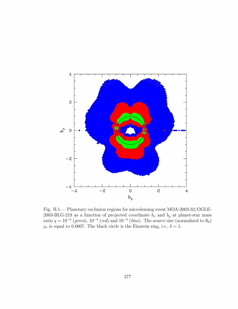
Fig. B.1.— Planetary exclusion regions for microlensing event MOA-2003-32/OGLE-2003-BLG-219 as a function of projected coordinate bx and by at planet-star massratio q = 10−5 (green), 10−4 (red) and 10−3 (blue). The source size (normalized to θE)ρ∗ is equal to 0.0007. The black circle is the Einstein ring, i.e., b = 1.

277

Appendix C

Extracting Orbital Parameters for Circular

Planetary Orbit

OGLE-2005-BLG-071 is the first planetary microlensing event for which the

effects of planetary orbital motion in the light curve have been fully analyzed. The

distortions of the light curve due to the orbital motion are modeled by ω and b as

discussed in § 4.3.2. In addition, the lens mass M and distance Dl are determined,

so we can directly convert the microlens light-curve parameters that are normalized

to the Einstein radius to physical parameters. In this section, we show that under

the assumption of a circular planetary orbit, the planetary orbital parameters can

be deduced from the light-curve parameters. Let r⊥ = DlθEd be the projected

star-planet separation and let r⊥γ be the instantaneous planet velocity in the

plane of the sky, i.e. r⊥γ⊥ = r⊥ω is the velocity perpendicular to this axis and

r⊥γ‖ = r⊥d/d is the velocity parallel to this axis. Let a be the semi-major axis and

define the ı, , k directions as the instantaneous star-planet-axis on the sky plane,

278

the direction into the sky, and k = ı × . Then the instantaneous velocity of the

planet is

v =

√

GM

a[cos θk + sin θ(cos φı − sin φ)], (C.1)

where φ is the angle between star-planet-observer (i.e., r⊥ = a sin φ) and θ is the

angle of the velocity relative to the k direction on the plane that is perpendicular to

the planet-star-axis. We thus obtain

γ⊥ =

√

GM

a3

cos θ

sin φ, γ‖ =

√

GM

a3sin θ cot φ. (C.2)

To facilitate the derivation, we define

A ≡ γ‖

γ⊥

= − tan θ cos φ, B ≡ r3⊥γ2

⊥

GM= cos2 θ sin φ, (C.3)

which yield as an equation for sin φ:

B = F (sin φ); F (x) =x(1 − x2)

A2 + 1 − x2. (C.4)

Note that F ′(sin φ) = 0 when sin2 φ∗ = (3/2)A2 + 1 − |A|√

(9/4)A2 + 2 . So

equation (C.4) has two degenerate solutions when B < F (sin φ∗) and has no

solutions when B > F (sin φ∗). Subsequently, one obtains,

a =r⊥

sin φ, cos i = − sin φ cos θ, K =

√

GM

aq sin i, (C.5)

279

where i is the inclination and K is the amplitude of radial velocity.

The Jacobian matrix used to transform from P (r⊥, γ⊥, γ‖) to P (a, φ, θ) is given

below,

∂(r⊥, γ⊥, γ‖)

∂(a, φ, θ)=

GM

a3

∣

∣

∣

∣

∣

sin φ a cos φ 0

− 32a

cos θsin φ

− cos θ cos φsin2 φ

− sin θsin φ

− 32a

sin θ cot φ − sin θsin2 φ

cos θ cot φ

∣

∣

∣

∣

∣

=GM

a3cot2 φ

(

1

2− sin2 θ tan2 φ

)

. (C.6)

Then for an arbitrary function H(a),

∂(r⊥, γ⊥, γ‖)

∂(H(a), cos φ, θ)=

∂(r⊥, γ⊥, γ‖)

∂(a, φ, θ)× 1

sin φH ′(a), (C.7)

which, for the special case of a flat distribution, H(a) = ln a, yields,

∂(r⊥, γ⊥, γ‖)

∂(ln(a), cos φ, θ)=

GM

r2⊥

cos2 φ

sin φ.(

1

2− sin2 θ tan2 φ

)

(C.8)

280

Appendix D

Failure of Elliptical-Source Models for

MOA-2007-BLG-400

Because MOA-2007-BLG-400 is the first microlensing event with a completely

buried caustic, it is important to rule out other potential causes of the deviations

seen in the light curve (apart from a planetary companion to the lens). The

principal features of these deviations are the twin “spikes” in the residuals, which are

approximately centered on the times when the lens enters and exits the source. In

the model, these crossings occur at about HJD’ = 4354.53 and HJD’ = 4354.63, i.e.,

very close to the spikes in Figure 2.1. In principle, one might be able to induce such

spikes by displacing the model source crossing times from the true times. The only

real way to achieve this (while still optimizing the overall fit parameters) would be if

the source were actually elliptical, but were modeled as a circle (which, of course, is

the norm).

One argument against this hypothesis is the similarity of the I and H residuals

(§ 2.3). If the source were an ellipsoidal variable, then one would expect color

gradients due to “gravity darkening”.

281

Nevertheless, we carried out two types of investigation of this possibility. First,

we modeled the light curve as an elliptical source magnified by a point (non-binary)

lens. In addition to the linear flux parameters (source flux plus blended flux for each

observatory) there are 6 model parameters, the three standard point-lens parameters

(t0, u0, tE), plus the source semimajor and semiminor axes (ρa, ρb) and the angle of

the source trajectory relative to the source major axis, α. We find that the elliptical

source reduces χ2 by about 200, but it does not remove the “spikes” from the

residuals, which was the primary motivation for introducing it. Instead, essentially

all of the χ2 improvement comes from eliminating the asymmetries from the rest

of the light curve. Recall, however, that the planetary model removes both these

asymmetries and the “spikes”. Moreover, the best-fit axis ratio is quite extreme,

ρb/ρa = 0.7, which would produce very noticeable ellipsoidal variations unless the

binary were being viewed pole on.

Next we looked for sinusoidal variations in the baseline light curve. The

individual OGLE errorbars at baseline are smaller than for MOA, and since

ellipsoidal variations are strictly periodic, the longer OGLE baseline (about

T = 2000 days versus T = 800 days for MOA) does a better job of isolating this

signal from various possible systematics. Therefore, for this purpose, the OGLE

data are more suitable than MOA. The OGLE data are essentially all baseline (only

two magnified points out of 452). Their periodogram shows several spikes at the

0.01 mag level, and a maximum ∆χ2 = 20, which are consistent with noise. The

282

width of the spikes is extremely narrow, consistent with the theoretical expectation

for uniformly sampled data of σ(P )/P 2 ∼√

24/∆χ2/(2πT ) ∼ 10−4 day−1, indicating

that the data set is behaving normally.

In brief, our investigation finds no convincing evidence for ellipticity of the

source, certainly not for the several tens of percent deviation from circular that

would be needed to significantly ameliorate the deviations seen near peak in the

light curve. Moreover, even arbitrary source ellipticities cannot reproduce the light

curve’s most striking features: the two “spikes” in the residuals that occur when the

lens crosses the source boundary.

283

BIBLIOGRAPHY

Abe, F., et al. 2004, Science, 305, 1264

Afonso, C., et al. 2000, ApJ, 532, 340

Afonso, C. et al. 2003, A&A, 400, 951

Albrow, M. D., et al. 1998, ApJ, 509, 687

Albrow, M. D., et al. 1999, ApJ, 512, 672

Albrow, M.D. et al. 1999, ApJ, 522, 1022

Albrow, M.D. et al. 2000, ApJ, 534, 894

Albrow, M. D., et al. 2000, ApJ, 535, 176

Albrow, M. D., et al. 2001, ApJ, 556, L113

Albrow, M. D., et al. 2002, ApJ, 572, 1031

Alcock, C. et al. 1993, Nature, 365, 621

Alcock, C. et al. 1995, ApJ, 454, L125

Alcock, C. et al. 1997, ApJ, 491, 436

Alcock, C. et al. 2000, ApJ, 542, 281

Alcock, C., et al. 2001, Nature, 414, 617

Alcock, C. et al. 2001, ApJ, 550, L169

An, J. H. 2005, MNRAS, 356, 1409

An, J. H. & Han, C. 2002, ApJ, 573, 351

An, J. H., et al. 2002, ApJ, 572, 521

284

Anderson, J. & King, I. R. 2004, Hubble Space Telescope Advanced Camera forSurveys Instrument Science Report 04-15

Assef, R. J. et al. 2006, ApJ, 649, 954

Aubourg, E. et al. 1993, Nature, 365, 623

Bailey, J., et al. 2009, ApJ, 690, 743

Bean, J. L., Benedict, G. F., & Endl, M. 2006, ApJ, 653, L65

Beaulieu, J.-P., et al. 2006, Nature, 439, 437

Benedict, G. F., et al. 2002, ApJ, 581, L115

Bennett, D. P., & Rhie, S. H. 1996, ApJ, 472, 660

Bennett, D. P., & Rhie, S. H. 2002, ApJ, 574, 985

Bennett, D. P., et al. 2006, ApJ, 647, L171

Bennett, D. P., Anderson, J., & Gaudi, B. S. 2007, ApJ, 660, 781

Bennett, D. P., et al. 1999, Nature, 402, 57

Bennett, D.P. et al., 2008, ApJ, 684, 663

Bessell, M. S., & Brett, J. M. 1988, PASP, 100, 1134

Bond, I. A., et al. 2001, MNRAS, 327, 868

Bond, I. A., et al. 2002, MNRAS, 333, 71

Bond, I. A., et al. 2004, ApJ, 606, L155

Boss, A. P. 2002, ApJ, 567, L149

Boss, A. P. 2006, ApJ, 643, 501

Boutreux, T. & Gould, A. 1996, ApJ, 462, 705

Brewer, B. J., & Lewis, G. F. 2005, MNRAS, 356, 703

Burrows, A., Hubbard, W. B., Saumon, D., & Lunine, J. I. 1993, ApJ, 406, 158

Burrows, A., et al. 1997, ApJ, 491, 856

Butler, R. P., et al. 2006, PASP, 118, 1685

Carpenter, J. 2001, AJ, 121, 2851

285

Calchi Novati, S., de Luca, F., Jetzer, P., & Scarpetta, G. 2006, A&A, 459, 407‘

Chang, K., & Refsdal, S. 1979, Nature, 282, 561

Chang, K. & Refsdal, S. 1984, A&A, 130, 157

Chung, S.-J., et al. 2005, ApJ, 630, 535

Claret, A. 2000, A&A, 363, 1081

Corrigan, R. T., et al. 1991, AJ, 102, 34

Cox, A. N. 2000, Allen’s Astrophysical Quantities (4th Ed.; New York; Springer)

Cumming, A., et al. 2008, PASP, 120, 531

Delfosse, X., et al. 1998, A&A, 338, L67

Demarque, P., Woo, J.-H., Kim, Y.-C., & Yi, S. K. 2004, ApJS, 155, 667

Dominik, M. 1999a, A&A, 341, 943

Dominik, M. 1999b, A&A, 349, 108

Dominik, M. 2006, MNRAS, 367, 669

Dong, S., et al. 2006, ApJ, 642, 842

Dong, S., et al. 2009, ApJ, 695, 970

Dong, S., et al. 2009, ApJ, 698, 1826

Doran, M., & Mueller, C. M. 2004, Journal of Cosmology and Particle Astrophysics,9, 3

Drake, A. J., Cook, K. H., & Keller, S. C. 2004, ApJ, 607, L29

Duquennoy, A., & Mayor, M. 1991, A&A, 248, 485

Einstein, A. 1936, Science, 84, 506

Eisenhauer, F., et al. 2005, ApJ, submitted (astro-ph/0502129)

Endl, M., et al. 2006, ApJ, 649, 436

European Space Agency, 1997, The Hipparcos and Tycho Catalogues (SP-1200;Noordwijk: ESA)

Fischer, D. A., & Valenti, J. 2005, ApJ, 622, 1102

286

Frank, S. et al. 2007, Astrophysics and Space Science, 312, 3

Gaudi, B. S., & Gould, A. 1997, ApJ, 486, 85

Gaudi, B. S., & Sackett, P. D. 2000, ApJ, 528, 56

Gaudi, B. S., et al. 2002, ApJ, 566, 463

Gaudi, B. S. 2008, Astronomical Society of the Pacific Conference Series, 398, 479,ed. D. Fischer, F. Rasio, S. Thorsett, & A. Wolszczan, Extreme Solar Systems(arXiv:0711.1614)

Gaudi, B. S., Naber, R. M., & Sackett, P. D. 1998, ApJ, 502, L33

Gaudi, B. S., et al. 2008, Science, 319, 927

Ghosh, H., et al. 2004, ApJ, 615, 450

Gould, A. 1992, ApJ, 392, 442

Gould, A. 1994a, ApJ, 421, L71

Gould, A. 1994b, ApJ, 421, L75

Gould, A. 1995, ApJ, 441, L21

Gould, A. 1999, ApJ, 514, 869

Gould, A. 2000a, ApJ, 535, 928

Gould, A. 2000b, ApJ, 542, 785

Gould, A. 2004, ApJ, 606, 319

Gould, A. 2008, ApJ, 681, 1593

Gould, A. 2009, Astronomical Society of the Pacific Conference Series, 403, 86,ed. K.Z. Stanek, The Variable Universe: A Celebration of Bohdan Paczynski(arXiv:0803.4324)

Gould, A. & An, J.H. 2002, ApJ, 565, 1381

Gould, A. & Gaucherel, C. 1997, ApJ, 477, 580

Gould, A., & Loeb, A. 1992, ApJ, 396, 104

Gould, A. & Salim, S. 1999 ApJ, 524, 794

Gould, A., Miralda-Escude, J., & Bahcall, J. N. 1994, ApJ, 423, L105

287

Gould, A., Stutz, A., & Frogel, J. A. 2001, ApJ, 547, 590

Gould, A., Bennett, D. P., & Alves, D. R., 2004, ApJ, 614, 404

Gould, A. et al. 2006, ApJ, 644, L37

Gould, A., Gaudi, B. S., & Bennett, D. P. 2007, NASA/NSF Exoplanet Task ForceWhite Paper (arXiv:0704.0767)

Gould, A., et al. 2009, ApJ, 698, L147

Griest, K. & Safizadeh, N. 1998, ApJ, 500, 37

Han, C. 2007, ApJ, 661, 1202

Han, C., & Gould, A. 1995, ApJ, 447, 53

Han, C. & Gould, A. 1996, ApJ, 467, 540

Han, C. & Gould, A. 2003, ApJ, 592, 172

Han, C., & Gaudi, B. S. 2008, ApJ, 689, 53

Hao, H., et al. 2007, ApJ, 659, 99

Harris, J. & Zaritsky, D. 2006, AJ, 131, 2514

Hauschildt, P. H., Allard, F., & Baron, E. 1999, ApJ, 512, 377

Haywood, M. 2008, A&A, 482, 673

Huchra, J. et al. 1985, AJ, 90, 691

Ida, S., & Lin, D. N. C. 2004, ApJ, 616, 567

Ida, S., & Lin, D. N. C. 2005, ApJ, 626, 1045

Jiang, G. et al. 2005, ApJ, 617, 1307

Johnson, J. A., et al. 2007a, ApJ, 665, 785

Johnson, J. A., et al. 2007b, ApJ, 670, 833

Kallivayalil, N., van der Marel, R. P., & Alcock, C. 2006, ApJ, 652, 1213

Kayser, R. et al. 1986, A&A, 166, 36

Kennedy, G. M., Kenyon, S. J., & Bromley, B. C. 2006, ApJ, 650, L139

Kennedy, G. M., & Kenyon, S. J. 2008, ApJ, 673, 502

288

Kervella, P., et al. 2004, A&A, 426, 297

King, I. 1962, AJ, 67, 471

Kiraga, M., & Paczynski, B. 1994, ApJ, 430, L101

Kochanek, C. S. 1996, ApJ, 473, 610

Kochanek, C. S. 2004, ApJ, 605, 58

Kornet, K., Wolf, S., & Rozyczka, M. 2006, A&A, 458, 661

Kozlowski, S., Wozniak, P. R., Mao, S., & Wood, A. 2007, ApJ, 671, 420

Kubas, D., et al. 2008, A&A, 483, 317

Lanzetta, K. M. et al. 1987, ApJ, 322, 739

Laughlin, G., Bodenheimer, P., & Adams, F. C. 2004, ApJ, 612, L73

Lecar, M., Podolak, M., Sasselov, D., & Chiang, E. 2006, ApJ, 640, 1115

Lejeune, T., Cuisinier, F., & Buser, R. 1997, A&AS, 125, 229

Lejeune, T., Cuisinier, F., & Buser, R. 1998, A&AS, 130, 65

Lewis, G. F., & Ibata, R. A. 1998, ApJ, 501, 478

Liebes, S., Jr. 1964, Phys.Rev., 133, 835

Lin, D. N. C., Bodenheimer, P., & Richardson, D. C. 1996, Nature, 380, 606

Lissauer, J. J. 1987, Icarus, 69, 249

Manfroid, J. 1995, A&AS, 113, 587

Mao, S., & Paczynski, B. 1991, ApJ, 374, L37

Marcy, G. W., et al 1998, ApJ, 505, L147

Marcy, G. W., et al 2001, ApJ, 556, 296

Mao, S. & Paczynski, B. 1991, ApJ, 374, L37

Mortonson, M. J. et al. 2005, ApJ, 628, 594

Nishiyama, S., et al. 2005, ApJ, 621, L105

Paczynski, B. 1986, ApJ, 304, 1

289

Park, B.-G. et al. 2004, ApJ, 609, 166

Park, B.-G., Jeon, Y.-B., Lee, C.-U., & Han, C. 2006, ApJ, 643, 1233

Pejcha, O., & Heyrovsky, D. 2009, ApJ, 690, 1772

Pollack, J. B., Hubickyj, O., Bodenheimer, P., Lissauer, J. J., Podolak, M., &Greenzweig, Y. 1996, Icarus, 124, 62

Poindexter, S. et al. 2005, ApJ, 633, 914

Prochter, G. E., et al. 2006, ApJ, 648, L93

Rasio, F. A., & Ford, E. B. 1996, Science, 274, 954

Rattenbury, N. J., Bond, I. A., Skuljan, J., & Yock, P. C. M. 2002, MNRAS, 335,159

Rauch, M. et al. 2002, ApJ, 576, 45

Reach, W. T., et al. 2005, PASP, 117, 978

Read, J.I., Wilkinson, M.I., Evans, N.W., Gilmore, G., Kleyna, J.T. 2006, MNRAS,366, 429

Refsdal, S. 1966, MNRAS, 134, 315

Reid, N. 1991, AJ, 102, 1428

Rhie, S. H., et al. 2000, ApJ, 533, 378

Rivera, E. J., et al. 2005, ApJ, 634, 625

Sackett, P. D. 1997, ESO Document: SPG-VLTI-97/002 (astro-ph/9709269)

Sahu, K. C., et al. 2001, Nature, 411, 1022

Sahu, K. C., Anderson, J., & King, I. R. 2002, ApJ, 565, L21

Santos, N. C., Israelian, G., & Mayor, M. 2004, A&A, 415, 1153

Schechter, P.L., Mateo, M. & Saha, A. 1993, PASP, 105 1342

Smith, M. C., Mao, S., & Paczynski, B. 2003, MNRAS, 339, 925

Stanek, K. Z., et al. 1997, ApJ, 477, 163

Stanimirovic, S. Staveley-Smith, L., & Jones, P.A. ApJ, 604, 176

Sumi, T. 2004, MNRAS, 349, 193

290

Tisserand, P. et al. 2007, A&A, 469, 387

Treyer, M., & Wambsganss, J. 2004, A&A, 416, 19

Udalski, A. 2003, Acta Astron., 53, 291

Udalski, A., et al. 1993, Acta Astronomica, 43, 289

Udalski, A., et al. 2005, ApJ, 628, L109

Walker, M. A. 1995, ApJ, 453, 37

Wambsganss, J. 1990, Ph.D. Thesis

Wambsganss, J. 2006, Saas-Fee Advanced Course 33: Gravitational Lensing: Strong,Weak and Micro, 453

Ward, W. R. 1997, Icarus, 126, 261

Witt, H. J. 1990, A&A, 236, 311

Wolszczan, A., & Frail, D. A. 1992, Nature, 355, 145

Wozniak, P. R. 2000, Acta Astron., 50, 421

Wozniak, et al. 2000, ApJ, 529, 88

Yoo, J., et al. 2004a, ApJ, 603, 139

Yoo, J., et al. 2004b, ApJ, 616, 1204

Yoo, J., Chaname, J., & Gould, A. 2004, ApJ, 601, 311

Zaritsky, D., Harris, J., Grebel, E.K., & Thompson, I.B. 2000, ApJ, 534, L53

Zibetti, S., et al. 2005, ApJ, 631, L105

291