Embed Size (px)
Citation preview
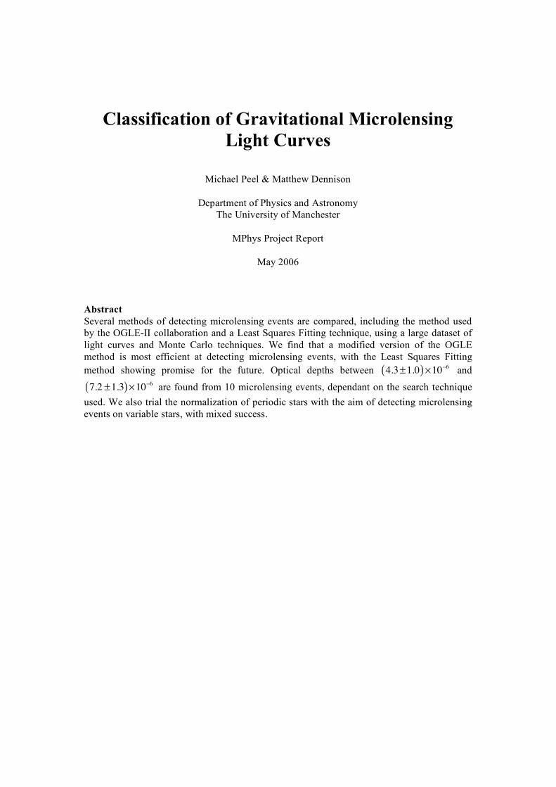
Classification of Gravitational Microlensing Light Curves
Michael Peel & Matthew Dennison
Department of Physics and Astronomy The University of Manchester
MPhys Project Report
May 2006
Abstract Several methods of detecting microlensing events are compared, including the method used by the OGLE-II collaboration and a Least Squares Fitting technique, using a large dataset of light curves and Monte Carlo techniques. We find that a modified version of the OGLE method is most efficient at detecting microlensing events, with the Least Squares Fitting method showing promise for the future. Optical depths between 4.3±1.0( )!10"6 and
7.2 ±1.3( )!10"6 are found from 10 microlensing events, dependant on the search technique used. We also trial the normalization of periodic stars with the aim of detecting microlensing events on variable stars, with mixed success.

Classification of Gravitational Microlensing Light Curves
2
1. Introduction Gravitational microlensing is the lensing of the light emitted from a source – either a star or another body emitting radiation – by an object with mass in the range of
10
!6M!" m "10
6M!
(Wambsganss 2004), where M!
is the solar mass, which passes through the line of sight between the source and Earth. The odds of a microlensing event occurring to a star within our galaxy at a particular time (known as the optical depth) is of the order of a million to one. This means that to have a reasonable chance of detecting a microlensing event, millions of stars have to be monitored. In the last decade, several groups have done this by regularly imaging crowded star fields such as the Galactic Bulge or the Large Magellanic Cloud, creating light curves of individual light sources within the star field, and searching through these light curves looking for signatures of microlensing events. This has resulted in thousands of microlensing events being detected. See section 3 of Wambsganss (2004) for a list and details of observing groups. In this project, we have used a data set of 174,693 light curves taken by the OGLE-III collaboration at 161 times between the 4th August 2001 and the 23rd September 2003. Woźniak (2000) provides details of the process used to obtain the light curve data from the raw CCD data. In the following Section, the theory of Gravitational Microlensing will be covered, and the equations used to model microlensing events and calculate the optical depth of microlensing will be given. Section 3 discusses the method of fitting this model to a microlensing event. Section 4 covers variable stars, and methods to remove the effects of variability. Section 5 covers the various methods used to identify microlensing events within the data set. Section 6 gives details of the microlensing events detected in the dataset. Section 7 concludes this report, and looks at future directions. A set of appendices are given at the end of this report, which contain the differentials used in the fitting methods (Appendix A), flow charts of the program structure (Appendix B) and a discussion of systematic errors (Appendix C). A DVD is also included with this report, which contains the data set used as well as graphs for each light curve, the program code and flow charts, and digital copies of the data presented in this report.
Classification of Gravitational Microlensing Light Curves
3
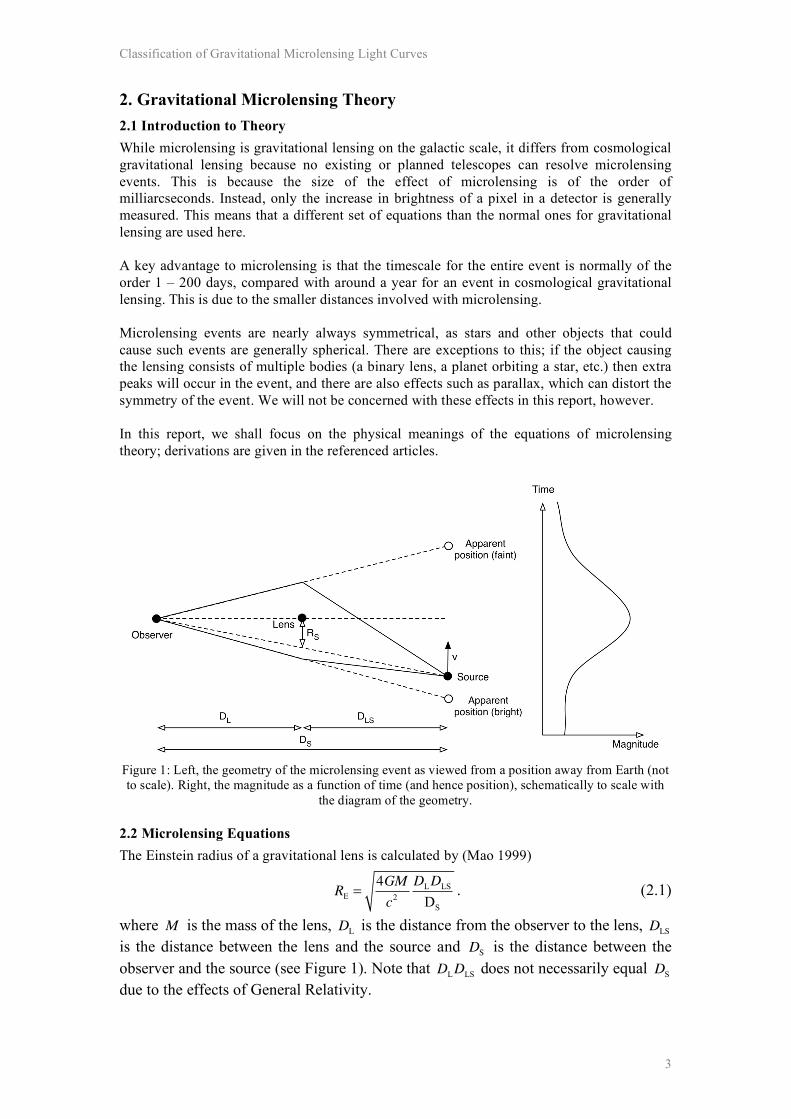
2. Gravitational Microlensing Theory 2.1 Introduction to Theory While microlensing is gravitational lensing on the galactic scale, it differs from cosmological gravitational lensing because no existing or planned telescopes can resolve microlensing events. This is because the size of the effect of microlensing is of the order of milliarcseconds. Instead, only the increase in brightness of a pixel in a detector is generally measured. This means that a different set of equations than the normal ones for gravitational lensing are used here. A key advantage to microlensing is that the timescale for the entire event is normally of the order 1 – 200 days, compared with around a year for an event in cosmological gravitational lensing. This is due to the smaller distances involved with microlensing. Microlensing events are nearly always symmetrical, as stars and other objects that could cause such events are generally spherical. There are exceptions to this; if the object causing the lensing consists of multiple bodies (a binary lens, a planet orbiting a star, etc.) then extra peaks will occur in the event, and there are also effects such as parallax, which can distort the symmetry of the event. We will not be concerned with these effects in this report, however. In this report, we shall focus on the physical meanings of the equations of microlensing theory; derivations are given in the referenced articles.
Figure 1: Left, the geometry of the microlensing event as viewed from a position away from Earth (not to scale). Right, the magnitude as a function of time (and hence position), schematically to scale with
the diagram of the geometry. 2.2 Microlensing Equations The Einstein radius of a gravitational lens is calculated by (Mao 1999)
RE=
4GM
c2
DLD
LS
DS
. (2.1)
where M is the mass of the lens, DL
is the distance from the observer to the lens, DLS
is the distance between the lens and the source and D
S is the distance between the
observer and the source (see Figure 1). Note that D
LD
LS does not necessarily equal
D
S
due to the effects of General Relativity.
Classification of Gravitational Microlensing Light Curves
4
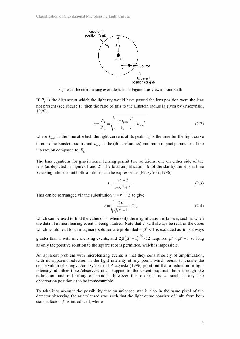
Figure 2: The microlensing event depicted in Figure 1, as viewed from Earth
If
R
S is the distance at which the light ray would have passed the lens position were the lens
not present (see Figure 1), then the ratio of this to the Einstein radius is given by (Paczyński, 1996).
r !RS
R E
=t " tpeak
tE
#
$%&
'(
2
+ umin
2 , (2.2)
where tpeak is the time at which the light curve is at its peak,
t
E is the time for the light curve
to cross the Einstein radius and u
min is the (dimensionless) minimum impact parameter of the
interaction compared to R
E.
The lens equations for gravitational lensing permit two solutions, one on either side of the lens (as depicted in Figures 1 and 2). The total amplification µ of the star by the lens at time t , taking into account both solutions, can be expressed as (Paczyński ,1996)
µ =r2+ 2
r r2+ 4
. (2.3)
This can be rearranged via the substitution v = r2 + 2 to give
r =2µ
µ2!1
! 2 , (2.4)
which can be used to find the value of r when only the magnification is known, such as when the data of a microlensing event is being studied. Note that r will always be real, as the cases which would lead to an imaginary solution are prohibited – µ2
<1 is excluded as µ is always
greater than 1 with microlensing events, and 2µ µ2!1( )
!12 < 2 requires µ2
< µ2!1 so long
as only the positive solution to the square root is permitted, which is impossible. An apparent problem with microlensing events is that they consist solely of amplification, with no apparent reduction in the light intensity at any point, which seems to violate the conservation of energy. Jaroszyński and Paczyński (1996) point out that a reduction in light intensity at other times/observers does happen to the extent required, both through the redirection and redshifting of photons, however this decrease is so small at any one observation position as to be immeasurable. To take into account the possibility that an unlensed star is also in the same pixel of the detector observing the microlensed star, such that the light curve consists of light from both stars, a factor
fl is introduced, where
Classification of Gravitational Microlensing Light Curves
5
fl=
Fl
Ful+ F
l
, (2.5)
in which F
l is the flux from the lensed star, and
F
ul the flux from the unlensed star. The
actual increase in luminosity measured by the pixel at time t is then
µB=µF
l+ F
ul
Fl+ F
ul
= µF
l
Fl+ F
ul
+F
ul
Fl+ F
ul
!
"#$
%&= µ f
l+ 1' f
l( ) , (2.6)
which goes to µ
B= µ when
fl= 1 , i.e. there is no unlensed star present.
Finally, the change in apparent magnitude of the star is given by
m = m
b! 2.5 log10 µB
, (2.7)
where m
b is the unlensed magnitude.
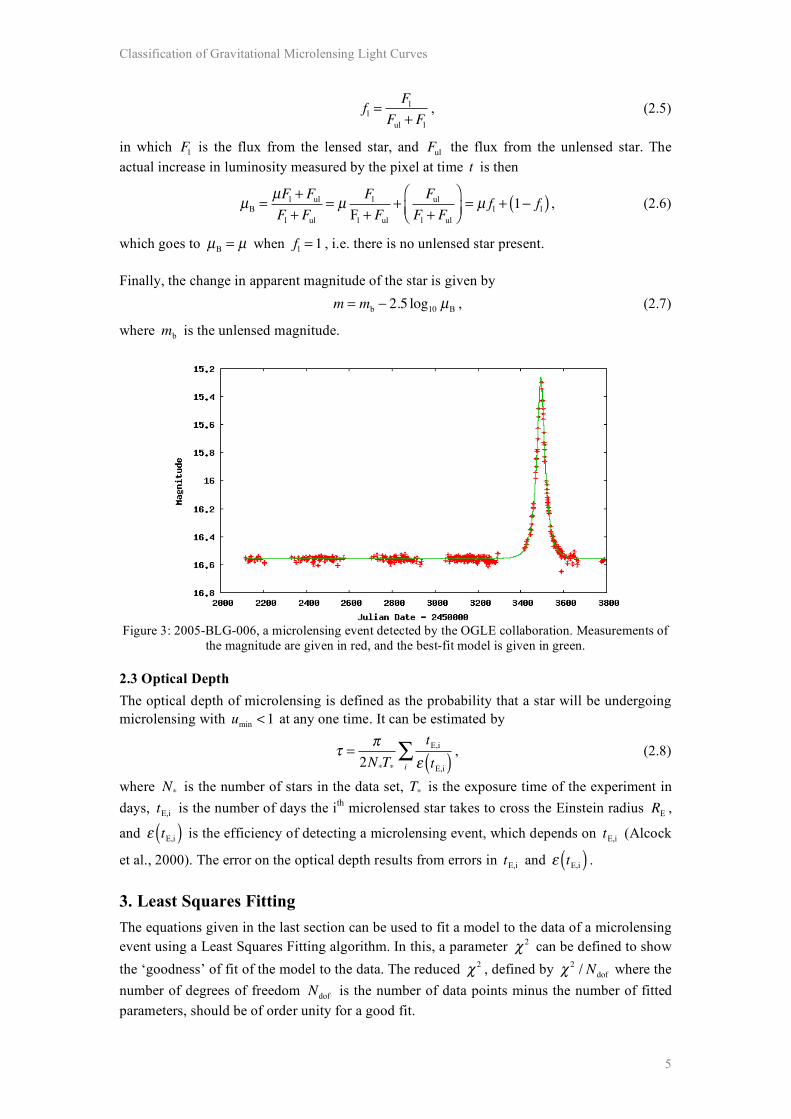
Figure 3: 2005-BLG-006, a microlensing event detected by the OGLE collaboration. Measurements of
the magnitude are given in red, and the best-fit model is given in green. 2.3 Optical Depth The optical depth of microlensing is defined as the probability that a star will be undergoing microlensing with
u
min<1 at any one time. It can be estimated by
! ="
2N*T*
tE,i
# tE,i( )i
$ , (2.8)
where N* is the number of stars in the data set, T
* is the exposure time of the experiment in
days, t
E,i is the number of days the ith microlensed star takes to cross the Einstein radius R
E,
and ! t
E,i( ) is the efficiency of detecting a microlensing event, which depends on t
E,i (Alcock
et al., 2000). The error on the optical depth results from errors in t
E,i and ! t
E,i( ) . 3. Least Squares Fitting
The equations given in the last section can be used to fit a model to the data of a microlensing event using a Least Squares Fitting algorithm. In this, a parameter ! 2 can be defined to show the ‘goodness’ of fit of the model to the data. The reduced ! 2 , defined by ! 2
/ Ndof
where the number of degrees of freedom
N
dof is the number of data points minus the number of fitted
parameters, should be of order unity for a good fit.
Classification of Gravitational Microlensing Light Curves
6
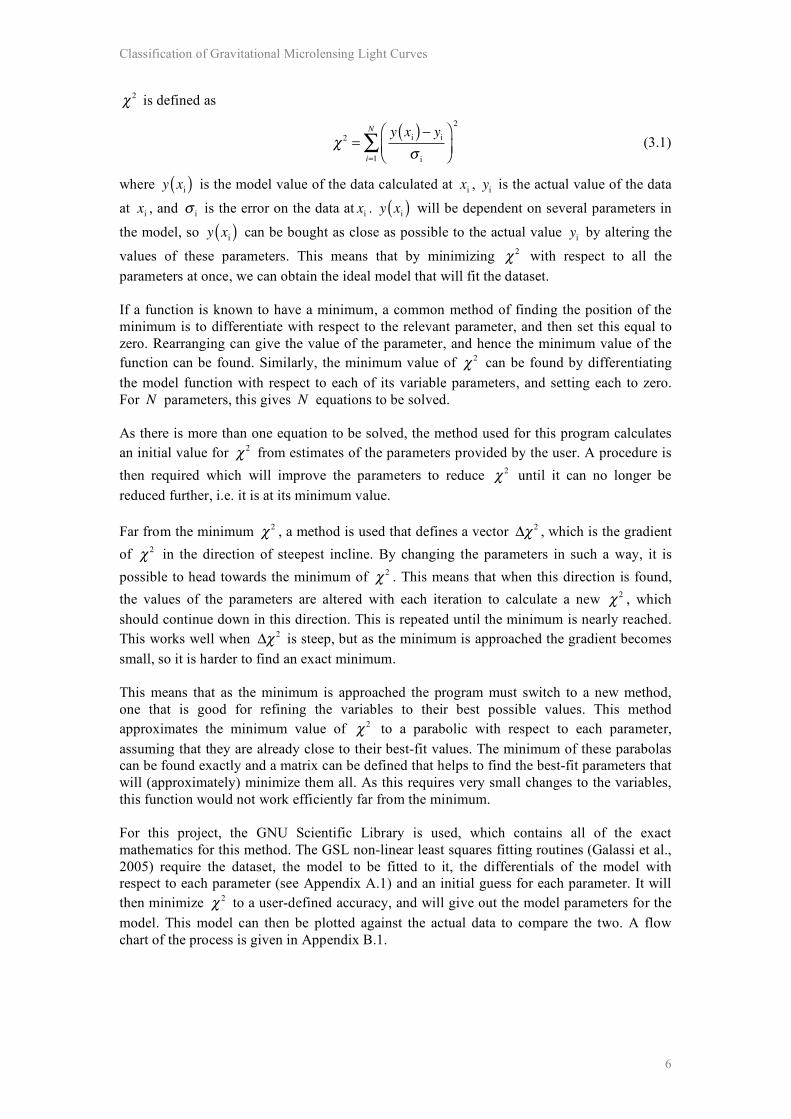
! 2 is defined as
! 2=
y xi( )" yi
#i
$
%&'
()
2
i=1
N
* (3.1)
where y x
i( ) is the model value of the data calculated at x
i,
y
i is the actual value of the data
at xi, and
!
i is the error on the data at x
i.
y x
i( ) will be dependent on several parameters in
the model, so y x
i( ) can be bought as close as possible to the actual value y
i by altering the
values of these parameters. This means that by minimizing ! 2 with respect to all the parameters at once, we can obtain the ideal model that will fit the dataset. If a function is known to have a minimum, a common method of finding the position of the minimum is to differentiate with respect to the relevant parameter, and then set this equal to zero. Rearranging can give the value of the parameter, and hence the minimum value of the function can be found. Similarly, the minimum value of ! 2 can be found by differentiating the model function with respect to each of its variable parameters, and setting each to zero. For N parameters, this gives N equations to be solved. As there is more than one equation to be solved, the method used for this program calculates an initial value for ! 2 from estimates of the parameters provided by the user. A procedure is then required which will improve the parameters to reduce ! 2 until it can no longer be reduced further, i.e. it is at its minimum value. Far from the minimum ! 2 , a method is used that defines a vector !" 2 , which is the gradient of ! 2 in the direction of steepest incline. By changing the parameters in such a way, it is possible to head towards the minimum of ! 2 . This means that when this direction is found, the values of the parameters are altered with each iteration to calculate a new ! 2 , which should continue down in this direction. This is repeated until the minimum is nearly reached. This works well when !" 2 is steep, but as the minimum is approached the gradient becomes small, so it is harder to find an exact minimum. This means that as the minimum is approached the program must switch to a new method, one that is good for refining the variables to their best possible values. This method approximates the minimum value of ! 2 to a parabolic with respect to each parameter, assuming that they are already close to their best-fit values. The minimum of these parabolas can be found exactly and a matrix can be defined that helps to find the best-fit parameters that will (approximately) minimize them all. As this requires very small changes to the variables, this function would not work efficiently far from the minimum. For this project, the GNU Scientific Library is used, which contains all of the exact mathematics for this method. The GSL non-linear least squares fitting routines (Galassi et al., 2005) require the dataset, the model to be fitted to it, the differentials of the model with respect to each parameter (see Appendix A.1) and an initial guess for each parameter. It will then minimize ! 2 to a user-defined accuracy, and will give out the model parameters for the model. This model can then be plotted against the actual data to compare the two. A flow chart of the process is given in Appendix B.1.
Classification of Gravitational Microlensing Light Curves
7
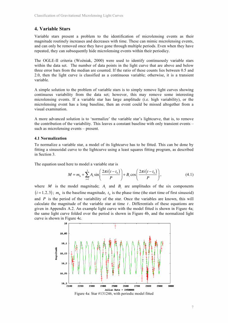
4. Variable Stars Variable stars present a problem to the identification of microlensing events as their magnitude routinely increases and decreases with time. These can mimic microlensing events, and can only be removed once they have gone through multiple periods. Even when they have repeated, they can subsequently hide microlensing events within their periodicy. The OGLE-II criteria (Woźniak, 2000) were used to identify continuously variable stars within the data set. The number of data points in the light curve that are above and below three error bars from the median are counted. If the ratio of these counts lies between 0.5 and 2.0, then the light curve is classified as a continuous variable; otherwise, it is a transient variable. A simple solution to the problem of variable stars is to simply remove light curves showing continuous variability from the data set; however, this may remove some interesting microlensing events. If a variable star has large amplitude (i.e. high variability), or the microlensing event has a long baseline, then an event could be missed altogether from a visual examination. A more advanced solution is to ‘normalize’ the variable star’s lightcurve, that is, to remove the contribution of the variability. This leaves a constant baseline with only transient events – such as microlensing events – present. 4.1 Normalization To normalize a variable star, a model of its lightcurve has to be fitted. This can be done by fitting a sinusoidal curve to the lightcurve using a least squares fitting program, as described in Section 3. The equation used here to model a variable star is
M = mb+ A
isin
2!i t " t0( )
P
#
$%&
'(+ B
icos
2!i t " t0( )
P
#
$%&
'(i=1
3
) , (4.1)
where M is the model magnitude; A
i and
B
i are amplitudes of the six components
i = 1,2, 3( ) ; m
b is the baseline magnitude, t
0 is the phase time (the start time of first sinusoid) and P is the period of the variability of the star. Once the variables are known, this will calculate the magnitude of the variable star at time t . Differentials of these equations are given in Appendix A.2. An example light curve with the model fitted is shown in Figure 4a; the same light curve folded over the period is shown in Figure 4b, and the normalized light curve is shown in Figure 4c.
Figure 4a: Star #131246, with periodic model fitted
Classification of Gravitational Microlensing Light Curves
8
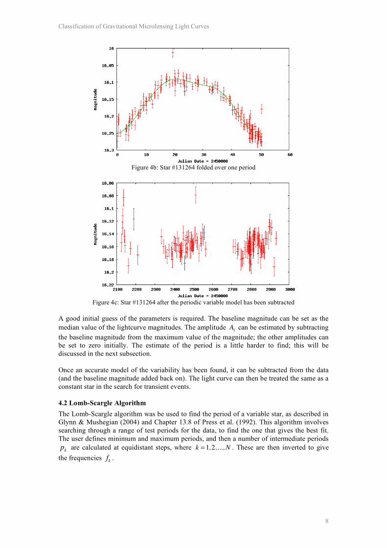
Figure 4b: Star #131264 folded over one period
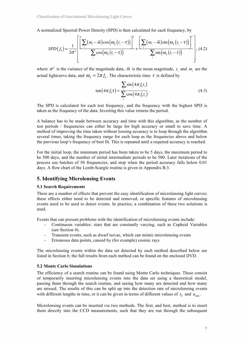
Figure 4c: Star #131264 after the periodic variable model has been subtracted
A good initial guess of the parameters is required. The baseline magnitude can be set as the median value of the lightcurve magnitudes. The amplitude A
1 can be estimated by subtracting
the baseline magnitude from the maximum value of the magnitude; the other amplitudes can be set to zero initially. The estimate of the period is a little harder to find; this will be discussed in the next subsection. Once an accurate model of the variability has been found, it can be subtracted from the data (and the baseline magnitude added back on). The light curve can then be treated the same as a constant star in the search for transient events. 4.2 Lomb-Scargle Algorithm The Lomb-Scargle algorithm was be used to find the period of a variable star, as described in Glynn & Mushegian (2004) and Chapter 13.8 of Press et al. (1992). This algorithm involves searching through a range of test periods for the data, to find the one that gives the best fit. The user defines minimum and maximum periods, and then a number of intermediate periods pk are calculated at equidistant steps, where k = 1,2,...,N . These are then inverted to give
the frequencies fk .
Classification of Gravitational Microlensing Light Curves
9
A normalized Spectral Power Density (SPD) is then calculated for each frequency, by
SPD fk( ) =
1
2! 2
mi" m( )cos #k
ti"$( )( )
i
%&
'(
)
*+
2
cos #kt
i"$( )( )
i
%+
mi" m( )sin #
kt
i"$( )( )
i
%&
'(
)
*+
2
sin #kt
i"$( )( )
i
%
&
'
(((((
)
*
+++++
, (4.2)
where ! 2 is the variance of the magnitude data, m is the mean magnitude, t
i and
m
i are the
actual lightcurve data, and ! k = 2" fk . The characteristic time ! is defined by
tan 4! fk"( ) =
sin 4! fkt
i( )i
#
cos 4! fkt
i( )i
#. (4.3)
The SPD is calculated for each test frequency, and the frequency with the highest SPD is taken as the frequency of the data. Inverting this value returns the period. A balance has to be made between accuracy and time with this algorithm, as the number of test periods / frequencies can either be large for high accuracy or small to save time. A method of improving the time taken without loosing accuracy is to loop through the algorithm several times, taking the frequency range for each loop as the frequencies above and below the previous loop’s frequency of best fit. This is repeated until a required accuracy is reached. For the initial loop, the minimum period has been taken to be 5 days, the maximum period to be 500 days, and the number of initial intermediate periods to be 500. Later iterations of the process use batches of 50 frequencies, and stop when the period accuracy falls below 0.01 days. A flow chart of the Lomb-Scargle routine is given in Appendix B.3. 5. Identifying Microlensing Events 5.1 Search Requirements There are a number of effects that prevent the easy identification of microlensing light curves; these effects either need to be detected and removed, or specific features of microlensing events need to be used to detect events. In practice, a combination of these two solutions is used. Events that can present problems with the identification of microlensing events include:
- Continuous variables: stars that are constantly varying, such as Cepheid Variables (see Section 4).
- Transient events, such as dwarf novae, which can mimic microlensing events - Erroneous data points, caused by (for example) cosmic rays
The microlensing events within the data set detected by each method described below are listed in Section 6; the full results from each method can be found on the enclosed DVD. 5.2 Monte Carlo Simulations The efficiency of a search routine can be found using Monte Carlo techniques. These consist of temporarily inserting microlensing events into the data set using a theoretical model, passing them through the search routine, and seeing how many are detected and how many are missed. The results of this can be split up into the detection rate of microlensing events with different lengths in time, or it can be given in terms of different values of
t
E and
u
min.
Microlensing events can be inserted via two methods. The first, and best, method is to insert them directly into the CCD measurements, such that they are run through the subsequent
Classification of Gravitational Microlensing Light Curves
10
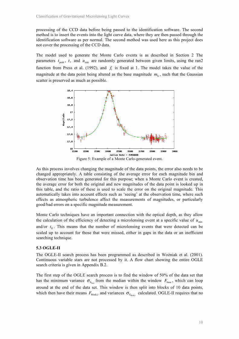
processing of the CCD data before being passed to the identification software. The second method is to insert the events into the light curve data, where they are then passed through the identification software as per normal. The second method was used here as this project does not cover the processing of the CCD data. The model used to generate the Monte Carlo events is as described in Section 2 The parameters
tpeak ,
t E and u
min are randomly generated between given limits, using the ran2
function from Press et al. (1992), and fl is fixed at 1. The model takes the value of the
magnitude at the data point being altered as the base magnitude m
b, such that the Gaussian
scatter is preserved as much as possible.
Figure 5: Example of a Monte Carlo-generated event.
As this process involves changing the magnitude of the data points, the error also needs to be changed appropriately. A table consisting of the average error for each magnitude bin and observation time has been generated for this purpose; when a Monte Carlo event is created, the average error for both the original and new magnitudes of the data point is looked up in this table, and the ratio of these is used to scale the error on the original magnitude. This automatically takes into account effects such as ‘seeing’ at the observation time, where such effects as atmospheric turbulence affect the measurements of magnitudes, or particularly good/bad errors on a specific magnitude measurement. Monte Carlo techniques have an important connection with the optical depth, as they allow the calculation of the efficiency of detecting a microlensing event at a specific value of u
min
and/or tE
. This means that the number of microlensing events that were detected can be scaled up to account for those that were missed, either in gaps in the data or an inefficient searching technique. 5.3 OGLE-II The OGLE-II search process has been programmed as described in Woźniak et al. (2001). Continuous variable stars are not processed by it. A flow chart showing the entire OGLE search criteria is given in Appendix B.2. The first step of the OGLE search process is to find the window of 50% of the data set that has the minimum variance
!
Fbase
from the median within the window F
base, which can loop
around at the end of the data set. This window is then split into blocks of 10 data points, which then have their means
F
block,i and variances !
Fblock,i calculated. OGLE-II requires that no
Classification of Gravitational Microlensing Light Curves
11
more than 2 of the block means can lie outside !
Fbase
of F
base (requirement 1), and that the
mean of the block variances is less than half of !
Fbase
(requirement 2),
!Fbase,i
i
"
N<1
2!
Fbase. (5.1)
Next, the number of data points within the whole data set that are within 1 sigma from the median, N
0!1", is counted, as well as the number of data points between 1 and 3 sigma,
N
1-3!.
For a Gaussian distribution around the median, which should be the case if the star’s luminosity is constant, these should have the relation
N1-3!
N0-1!
"32
68. (5.2)
If they do not, then this is an indication that some variability is occurring. This ratio is used to define a threshold ! ,
! = " Fbase#max
N1-3" / N0-1"
32 / 68,1
$%&
'()#max
" Fbase
" ph
,1$%*
&*
'(*
)*. (5.3)
In the program described in this report, the last term has been ignored as the value of ! ph -
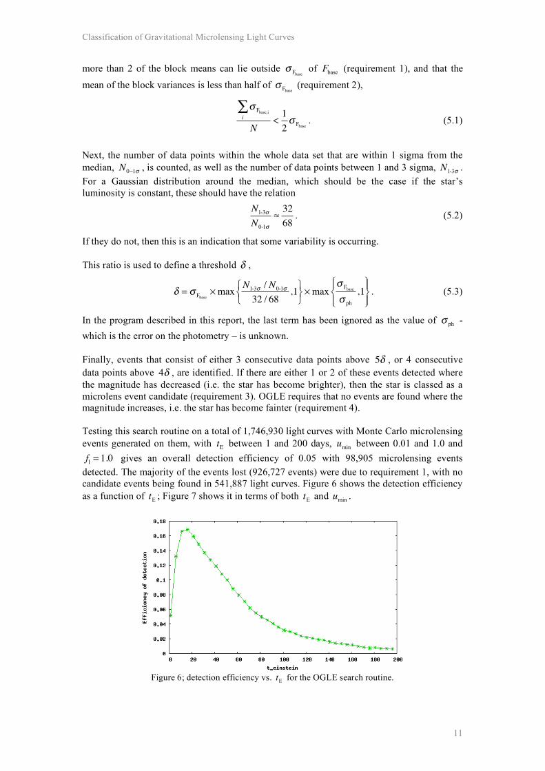
which is the error on the photometry – is unknown. Finally, events that consist of either 3 consecutive data points above 5! , or 4 consecutive data points above 4! , are identified. If there are either 1 or 2 of these events detected where the magnitude has decreased (i.e. the star has become brighter), then the star is classed as a microlens event candidate (requirement 3). OGLE requires that no events are found where the magnitude increases, i.e. the star has become fainter (requirement 4). Testing this search routine on a total of 1,746,930 light curves with Monte Carlo microlensing events generated on them, with t
E between 1 and 200 days, u
min between 0.01 and 1.0 and
fl= 1.0 gives an overall detection efficiency of 0.05 with 98,905 microlensing events
detected. The majority of the events lost (926,727 events) were due to requirement 1, with no candidate events being found in 541,887 light curves. Figure 6 shows the detection efficiency as a function of
t
E; Figure 7 shows it in terms of both
t
E and
u
min.
Figure 6; detection efficiency vs.
t
E for the OGLE search routine.
Classification of Gravitational Microlensing Light Curves
12
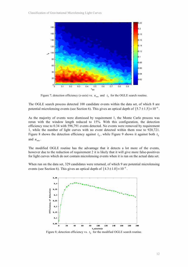
Figure 7; detection efficiency (z-axis) vs. u
min and
t
E for the OGLE search routine.
The OGLE search process detected 100 candidate events within the data set, of which 8 are potential microlensing events (see Section 6). This gives an optical depth of 5.7 ±1.5( )!10"6 . As the majority of events were dismissed by requirement 1, the Monte Carlo process was rerun with the window length reduced to 15%. With this configuration, the detection efficiency rose to 0.34 with 596,791 events detected. No events were removed by requirement 1, while the number of light curves with no event detected within them rose to 920,721. Figure 8 shows the detection efficiency against
t
E, while Figure 9 shows it against both
t
E
and umin
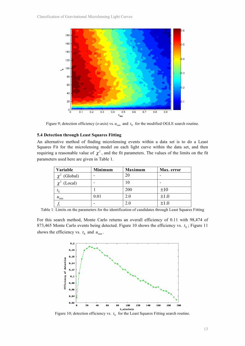
. The modified OGLE routine has the advantage that it detects a lot more of the events, however due to the reduction of requirement 2 it is likely that it will give more false-positives for light curves which do not contain microlensing events when it is run on the actual data set. When run on the data set, 329 candidates were returned, of which 9 are potential microlensing events (see Section 6). This gives an optical depth of 4.3±1.0( )!10"6 .
Figure 8; detection efficiency vs. t
E for the modified OGLE search routine.
Classification of Gravitational Microlensing Light Curves
13
Figure 9; detection efficiency (z-axis) vs. u
min and t
E for the modified OGLE search routine.
5.4 Detection through Least Squares Fitting An alternative method of finding microlensing events within a data set is to do a Least Squares Fit for the microlensing model on each light curve within the data set, and then requiring a reasonable value of ! 2 , and the fit parameters. The values of the limits on the fit parameters used here are given in Table 1.
Variable Minimum Maximum Max. error ! 2 (Global) - 20 -
! 2 (Local) - 10 -
t
E 1 200 ±10
u
min 0.01 2.0 ±1.0
fl - 2.0 ±1.0
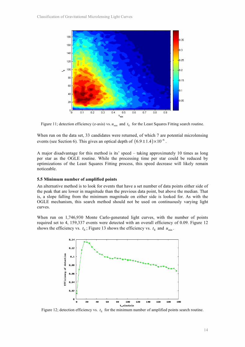
Table 1: Limits on the parameters for the identification of candidates through Least Squares Fitting For this search method, Monte Carlo returns an overall efficiency of 0.11 with 98,474 of 873,465 Monte Carlo events being detected. Figure 10 shows the efficiency vs. t
E; Figure 11
shows the efficiency vs. tE
and umin
.
Figure 10; detection efficiency vs. t
E for the Least Squares Fitting search routine.
Classification of Gravitational Microlensing Light Curves
14
Figure 11; detection efficiency (z-axis) vs. u
min and t
E for the Least Squares Fitting search routine.
When run on the data set, 33 candidates were returned, of which 7 are potential microlensing events (see Section 6). This gives an optical depth of 6.9 ±1.4( )!10"6 . A major disadvantage for this method is its’ speed – taking approximately 10 times as long per star as the OGLE routine. While the processing time per star could be reduced by optimizations of the Least Squares Fitting process, this speed decrease will likely remain noticeable. 5.5 Minimum number of amplified points An alternative method is to look for events that have a set number of data points either side of the peak that are lower in magnitude than the previous data point, but above the median. That is, a slope falling from the minimum magnitude on either side is looked for. As with the OGLE mechanism, this search method should not be used on continuously varying light curves. When run on 1,746,930 Monte Carlo-generated light curves, with the number of points required set to 4, 159,337 events were detected with an overall efficiency of 0.09. Figure 12 shows the efficiency vs. t
E; Figure 13 shows the efficiency vs. t
E and u
min.
Figure 12; detection efficiency vs. t
E for the minimum number of amplified points search routine.
Classification of Gravitational Microlensing Light Curves
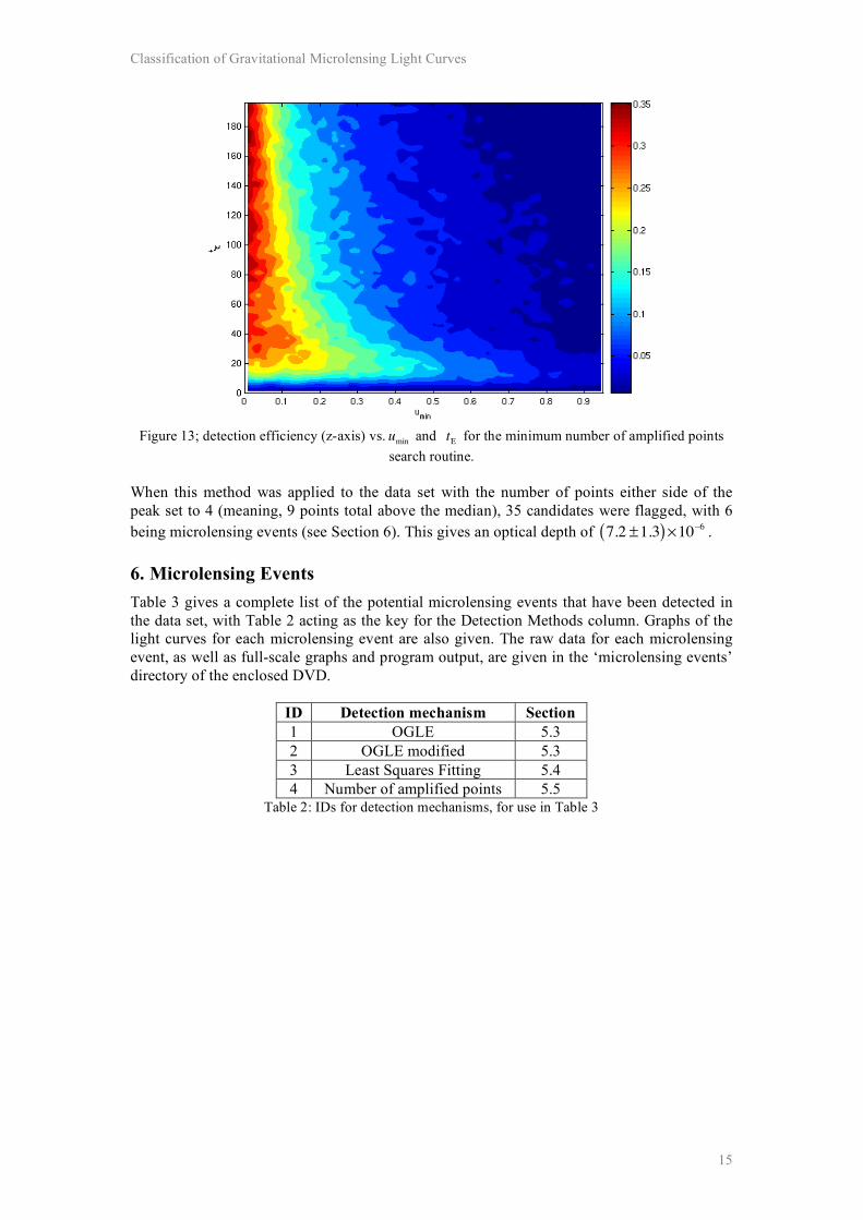
15
Figure 13; detection efficiency (z-axis) vs. u
min and t
E for the minimum number of amplified points
search routine. When this method was applied to the data set with the number of points either side of the peak set to 4 (meaning, 9 points total above the median), 35 candidates were flagged, with 6 being microlensing events (see Section 6). This gives an optical depth of 7.2 ±1.3( )!10"6 . 6. Microlensing Events Table 3 gives a complete list of the potential microlensing events that have been detected in the data set, with Table 2 acting as the key for the Detection Methods column. Graphs of the light curves for each microlensing event are also given. The raw data for each microlensing event, as well as full-scale graphs and program output, are given in the ‘microlensing events’ directory of the enclosed DVD.
ID Detection mechanism Section 1 OGLE 5.3 2 OGLE modified 5.3 3 Least Squares Fitting 5.4 4 Number of amplified points 5.5
Table 2: IDs for detection mechanisms, for use in Table 3