A&A 564, A109 (2014)DOI: 10.1051/0004-6361/201322430c© ESO 2014

Astronomy&

Astrophysics

MyGIsFOS: an automated code for parameter determinationand detailed abundance analysis in cool stars�

L. Sbordone1,2, E. Caffau1,2,��, P. Bonifacio2, and S. Duffau1

1 Zentrum für Astronomie der Universität Heidelberg, Landessternwarte, Königstuhl 12, 69117 Heidelberg, Germanye-mail: lsbordon@lsw.uni-heidelberg.de

2 GEPI, Observatoire de Paris, CNRS, Université Paris Diderot, place Jules Janssen, 92190 Meudon, France

Received 2 August 2013 / Accepted 20 November 2013

ABSTRACT

Context. The current and planned high-resolution, high-multiplexity stellar spectroscopic surveys, as well as the swelling amount ofunderutilized data present in public archives, have led to an increasing number of efforts to automate the crucial but slow process ofretrieving stellar parameters and chemical abundances from spectra.Aims. We present MyGIsFOS1, a code designed to derive atmospheric parameters and detailed stellar abundances from medium- tohigh-resolution spectra of cool (FGK) stars. We describe the general structure and workings of the code, present analyses of a numberof well-studied stars representative of the parameter space MyGIsFOS is designed to cover, and give examples of the exploitation ofMyGIsFOS very fast analysis to assess uncertainties through Monte Carlo tests.Methods. MyGIsFOS aims to reproduce a “traditional” manual analysis by fitting spectral features for different elements against aprecomputed grid of synthetic spectra. The lines of Fe i and Fe ii can be employed to determine temperature, gravity, microturbulence,and metallicity by iteratively minimizing the dependence of Fe i abundance from line lower energy and equivalent width, and imposingFe i-Fe ii ionization equilibrium. Once parameters are retrieved, detailed chemical abundances are measured from lines of otherelements.Results. MyGIsFOS replicates closely the results obtained in similar analyses on a set of well-known stars. It is also quite fast,performing a full parameter determination and detailed abundance analysis in about two minutes per star on a mainstream desktopcomputer. Currently, its preferred field of application are high-resolution and/or large spectral coverage data (e.g., UVES, X-shooter,HARPS, Sophie).

Key words. methods: data analysis – techniques: spectroscopic – stars: fundamental parameters – stars: abundances

1. Introduction

The availability of several high-efficiency, high-multiplexityspectrographs has brought about the need to perform accurateabundance analysis on large sets of stellar spectra of low tohigh resolution. The problem has been tackled in many dif-ferent ways, one may roughly divide the methods into global,which make use of the whole spectrum (e.g., Katz et al. 1998;Allende Prieto et al. 2000; Bailer-Jones 2000; Recio-Blancoet al. 2006) and local, that make use only of selected sections ofthe spectrum (e.g., Erspamer & North 2002; Bonifacio & Caffau2003; Barklem et al. 2005; Boeche et al. 2011; Posbic et al.2012; Mucciarelli et al. 2013; Magrini et al. 2013). A few in-termediate cases exist, most notably SME (Spectroscopy MadeEasy, Valenti & Piskunov 1996; Barklem et al. 2005), underlin-ing perhaps the difficulty of coming up with a clear-cut classifi-cation scheme. Complex pipelines, like that of the Sloan DigitalSky Survey (Allende Prieto et al. 2008), use multiple meth-ods whose results are then suitably combined. Among the localcodes one may distinguish between those that rely on equivalentwidths (EWs) measured by automatic codes such as fitline(François et al. 2003), DAOSPEC (Stetson & Pancino 2008) orARES (Sousa et al. 2007) to determine stellar parameters andabundances (GALA, FAMA, Mucciarelli et al. 2013; Magriniet al. 2013), and those that rely on line fitting (Erspamer & North2002; Bonifacio & Caffau 2003; Barklem et al. 2005; Boecheet al. 2011; Posbic et al. 2012; Van der Swaelmen et al. 2013).

� My God It’s Full Of Stars, http://mygisfos.obspm.fr�� Gliese Fellow.

Allende Prieto (2004) argued that EW based analysis should beabandoned; see also Bonifacio (2005) on EWs and line fitting.

We present in this paper the code MyGIsFOS that usesa local approach to treat large numbers of medium- to high-resolution spectra. Among the local codes MyGIsFOS, Abbo(Bonifacio & Caffau 2003), and the RAVE pipeline of Boecheet al. (2011) are the only ones, to our knowledge, that do notperform on-the-fly line transfer computations, but rely only on aprecomputed grid. In the Boeche et al. (2011) pipeline, a libraryof synthetic curves of growth are compared to the measured EWof the chosen observed lines. In this sense, this code is closer toEW-based codes as far as line selection criteria, advantages, andlimitations are concerned, but faster than most EW-based codessince no on-the-fly line transfer is performed.

On the other hand, MyGIsFOS and Abbo directly fit the syn-thetic profile of each chosen feature against the observed one.As such, they allow us to circumvent some of the limitations ofEW-based codes (see, e.g., Sect. 5.1), while, at the same time,maintaining the speed advantage of codes not performing on-the-fly calculations.

At the same time, the RAVE pipeline, MyGIsFOS, and Abbosuffer limitations inherent to the use of pre-computed grids.Namely, these grids can become exceedingly large, or must belimited in parameter space range. Moreover, precomputed gridsare by their nature rigid: their computation is resource intensive,and recomputation for the purpose of changing, for instance, theoscillation strengths of a couple of lines might not be a desirableoption.

Article published by EDP Sciences A109, page 1 of 15

A&A 564, A109 (2014)

For all these reasons, such codes are optimized to analyzea large number of stars that span a limited range in metallicity,effective temperature, and surface gravity.

MyGIsFOS specifically targets the treatment of largeamounts of data, through a local approach, based on spectrumsynthesis, line profile fitting, and a precomputed synthetic spec-trum grid. Although other procedures exist that incorpoaratethese features, none exists that uses all of these features at thesame time. In this case we believe MyGIsFOS is unique andinnovative.

2. The purpose of MyGIsFOS

MyGIsFOS is built on the foundation of our previous au-tomatic abundance analysis code Abbo (Bonifacio & Caffau2003). Although we have completely rewritten the code with adifferent input-output system, and it is now considerably morepowerful and faster, the scope of the code is unchanged withrespect to Abbo. Broadly speaking, we compare the observedspectrum against a suitable grid of synthetic stellar spectra whichwe computed at varying Teff , log g, Vturb, [Fe/H], and [α/Fe].Selected Fe i, Fe ii, and α-elements features are used to itera-tively estimate the best values for each parameter, after whichfeatures for other elements are fitted to derive the correspondingabundances.

MyGIsFOS is conceived to strictly replicate a classical ormanual procedure to derive stellar atmospheric parameters anddetailed chemical abundances from high-resolution stellar spec-tra of cool stars. As such, its most typical usage can be summa-rized as follows:

– For each star to be analyzed, the user provides input observedspectrum and a set of first guess parameters.

– The user provides the code a feature list, i.e., a list of spectralintervals for the grid to be fitted against the observed spec-trum. In the most general case, the feature list will includecontinuum intervals for pseudonormalization and signal-to-noise ratio (S/N) estimation, intervals corresponding to Fe i,Fe ii, and α-element lines for atmospheric parameter andmetallicity ([Fe/H]) determination, and intervals correspond-ing to lines of other elements for the determination of de-tailed abundances.

– Teff is determined from a set of isolated Fe i lines imposingthe linear fit of the transition lower energy vs. line abundanceto have null slope (for brevity, we will henceforth refer to thisquantity as lower energy abundance slope, or LEAS).

– Vturb is determined by imposing null slope for the EW vs.abundance relation of isolated Fe i lines.

– log g is determined from Fe i–Fe ii ionization equilibrium.– Fe abundance is determined from Fe i lines only.– [α/Fe] is determined by measuring lines of various α el-

ements, and using their average [X/Fe] as an estimate of[α/Fe].

– Vturb, log g, and [α/Fe] are estimated iteratively, in a nestedfashion, [α/Fe] being the outermost “shell”, Vturb the inner-most. For a given set of current guesses of Teff, log g, and αenhancement, Vturb is determined, then the code proceeds toupdate the gravity estimate: if the current one is not appropri-ate, a new one is guessed, Vturb is redetermined by assumingthe new gravity and the existing estimates for the other pa-rameters, then gravity is tested again. When a satisfactoryestimate is reached for both Vturb and log g, [α/Fe] is tested,and if changed, a recalculation of Vturb and log g is triggered.

– Teff is evaluated in a slightly different fashion: initially, theaforementioned analysis is repeated to full convergence as-suming a set of different temperatures, and in each case, theLEAS is derived. This intial mapping is used to fit the Teff-LEAS relationship and to look for a zero-slope temperature,which is then used to repeat the Vturb, log g, [α/Fe] determi-nation. The LEAS is evaluated again and the estimated slopeis added to the Teff-LEAS relationship fitting sample. A zerois searched again and so on, until convergence is reached.

– Any of the aforementioned parameters can be either derivedas described from the spectrum, or kept fixed at a user-defined value. MyGIsFOS will, of course, refrain from al-tering parameters for which the corresponding estimator isabsent (e.g., gravity will not be estimated if no Fe ii featuresare successfully measured). Thus, the user does not need toprovide features for any parameter he/she is not planning toalter, the only exception being Fe i features, which shouldalways be present ([Fe/H] cannot be kept fixed).

– The whole analysis is executed in a fully automated way forall the stars in the input list and the output is stored in a sepa-rate directory for each star. The input star list should containdata of similar quality and spectral range (e.g., UVES red-arm spectra with S /N ∼ 50−100; for a description of UVES,see Dekker et al. 2000), and of objects of comparable char-acteristics (say, metal-rich FGK dwarfs) because feature list,general running parameters (e.g., fit rejection tolerances) andsynthetic spectra grid are common to the input star list andshould thus be appropriate for all the objects. The constraintson S/N, spectral type and metallicity, are not very tight.Experiments with real UVES spectra have shown that if thefeature list has been optimized for S/N in the range 50−100 itcan work well for S/N in the ratio 15−300. At a low S/N mostof the selected features are not detected because they are tooweak and the user has to switch to a selection of strong, sat-urated lines. At the high S/N end it is useful to add manyweak lines that are not detectable at lower S/N. For atmo-spheric parameters, the main constraint is metallicity, sincefeatures that are heavily blended become much cleaner andare usable at lower metallicity; at the same time, features thatare saturated in the high-metallicity regime reach the linearpart of the curve of growth at lower metallicity. The switch-over between a metal-rich and metal-weak regime happenssomewhere between [M/H] −0.5 and −1.0. MyGIsFOS isdesigned to analyze data sets for which we have some pre-vious knowledge (colors, metallicity estimates, membershipto a cluster or dwarf galaxy). Our experience is that in thesecases the stars that need to be rerun a second time becausethey are initially misclassified are less than 5% of the total.

It is then clear that the ideal application of MyGIsFOS is thedetermination of detailed chemical abundances from high- tointermediate-resolution spectra of cool stars with basically thesame limitations and strengths as a traditional manual analy-sis: the results will be of higher quality if the spectral cover-age is large, if S/N is good, and if clean, unblended features arechosen. Few, noisy, or unreliable Fe ii lines will make gravityestimation difficult, the quality of the adopted atomic data im-pacts the precision of any abundance derived, and so on. Onthe other hand, MyGIsFOS results are immediately compara-ble with the results derived from a traditional abundance anal-ysis. Uncertainties, limitations, and dependence on the assump-tion made in atmosphere modeling and spectrosynthesis are wellknown, and researchers in the field are long since used to dealingwith them. This makes MyGIsFOS output easy to test, interpret,

A109, page 2 of 15

L. Sbordone et al.: A code for automatic abundance analysis

Table 1. The MyGIsFOS grids computed with SYNTHE and ATLAS 12 models employed for the present paper.

Grid Teff log g Vturb [Fe/H] [α/Fe] Number ofname range range range range range models

[K] [c.g.s.] [km s−1]Metal poor cool dwarfs 5000 to 6000 3 to 5 0 to 3 –4 to –0.5 –0.4 to 0.8 3840(MPCD) step 200 K step 0.5 step 1 step 0.5 step 0.4

Metal rich cool dwarfs 5000 to 6000 3 to 5 0 to 3 –1 to 0.75 –0.4 to 0.8 3840(MRCD) step 200 K step 0.5 step 1 step 0.25 step 0.4

Metal poor giants 4200 to 5600 1 to 3 1 to 3 –4 to –0.5 –0.4 to 0.4 2880(MPG) step 200 K step 0.5 step 1 step 0.5 step 0.4

Metal rich giants 4200 to 5600 1 to 3 1 to 3 –1 to 0.5 –0.4 to 0.4 2520(MRG) step 200 K step 0.5 step 1 step 0.25 step 0.4

and compare with the results from previous works, which areadvantages that MyGIsFOS shares with EW-based automationschemes such as FAMA or GALA.

MyGIsFOS produces an extensive output (in ASCII format)for each star to allow for critical examination of the analysisoutcome. Included is detailed information on each feature fit-ted (best fitting line profile, abundance, EW, rejection flags andquality-of-fit estimators), pseudonormalized input spectra andbest-fitting synthetic spectra, as well as averaged abundancesand parameters in tabular form, and a full listing of all the in-put parameters, employed grid characteristics, and code version.Also, all output files from the same run share a timestamp to easetracking.

Thanks to the use of a fully precomputed synthetic grid,MyGIsFOS is remarkably fast: a typical run on a standard desk-top computer, with full parameter determination and ∼20 el-ement abundances, for 200 nm high-resolution optical spectratakes about 120 s per star (see Sect. 8 for more details).

3. The synthetic spectra grid

MyGIsFOS works by comparing selected spectral features witha grid of synthetic stellar spectra with varying Teff , log g, Vturb,[Fe/H], and [α/Fe]. The grid is provided as an unformatted bi-nary file that reduces physical size and read-in time. The gridcontains a header containing a comment, the grid metrics (start-ing point, step, and number of steps in each parameter), the as-sumed solar abundances, the elements affected by α enhance-ment and the assumed grid instrumental broadening. The gridshould be fed to MyGIsFOS already broadened as needed by thespectrograph resolution. The grid is divided into several spectralranges or frames. This is foreseen to handle situations in whichonly limited, noncontiguous spectral ranges are needed, such aswhen treating data from different settings of single-order, high-multiplexity spectrographs such as VLT/FLAMES1 (Pasquiniet al. 2002). If this is not needed, the grid might contain a singleframe covering the needed spectral range. The frame subdivisionis also indicated in the grid header, which contains all the infor-mation needed by MyGIsFOS to read in the grid data withoutuser intervention. The grid should be passed to MyGIsFOS athigh sampling (Δλ/λ > 100 000) to prevent the introduction

1 Apart from the savings in file size, this allows the user to apply dif-ferent instrumental broadening values to each frame as they are needed,e.g., for different VLT/FLAMES settings or VLT/X-shooter spectralarms.

of artifacts when it is resampled over the actual observed datapoints.

For all the tests presented in this paper, we computed a setof model atmospheres and synthetic spectra appropriate for theanalysis of FGK stars, both dwarfs and giants, over a wide rangeof metallicities. The atmospheric models were computed withthe Linux version of ATLAS 12, while synthetic spectra cover-ing the UVES RED 580 setting (approx 480 to 680 nm) werecomputed by means of SYNTHE (Kurucz 2005; Castelli 2005;Sbordone et al. 2004; Sbordone 2005). Parameter space cover-age of the used grids to date are listed in Table 1. We computedmodels and syntheses in a self-consistent way, i.e. by includ-ing changes in Vturb and [α/Fe] already in the opacity computa-tion during model calculation. We took solar abundances fromCaffau et al. (2011b) for the elements there analyzed, and fromLodders et al. (2009) for the remaining species. The grids usedare part of a larger set currently being prepared for publication(Sbordone et al., in prep.). Synthetic grids are computed withsampling Δλ/λ = 300 000 in the 460−690 nm range, and take intheir binary packaged version between 1.5 and 2.2 GB of space.

4. The MyGIsFOS workflow in detail

As stated above, MyGIsFOS replicates classical manual abun-dance analysis workflow. User defined parameters are read froman ASCII parameter file. A flowchart of the process for a singlestar is shown in Fig.1, while an example of the result is given inFig. 2. The workflow can be summarized as follows:

1. The observed spectrum (or spectra) is pseudonormalized byevaluating the pseudo-median of each continuum interval2.A continuum value is then calculated for each observed pixelby computing a spline through all the continuum intervals.Also, from every continuum interval the local S/N is esti-mated. The whole synthetic grid is pseudonormalized in thesame way. The pseudonormalization is kept fixed throughoutthe analysis of the star.

2 Given a vector of N values, the median is defined as the value at theN/2-th element of the sorted vector. The pesudomedian employed byMyGIsFOS is instead the value at the N/a-th element of the sorted vec-tor. It is thus equivalent to the true median for a = 2, but the most typicalvalues employed in MyGIsFOS are in the range a = 1.25−1.66: this isdone to account for the fact that in most cases the chosen continuumintervals correspond more exactly to pseudocontinua, where weak linesare buried into the noise so that the use of a straight average or medianwould underestimate the continuum value. It is left to the user to fix theproper pseudomedian factor a by visually inspecting the spectra.

A109, page 3 of 15

A&A 564, A109 (2014)

Fig. 1. A schematic flowchart of MyGIsFOS. Numbers in rectangles refer to the MyGIsFOS phases enumeration given in Sect. 4.

Fig. 2. A small section of the S /N = 50 solar spectrum presented in 6.1 with overplotted MyGIsFOS features and fitting result as produced by theancillary plotting package SQUID. From left to right: a rejected Na i line (rejected due to EW exceeding the applied maximum EW constraint,gray shaded box); a Ti i feature (green box); a continuum interval (gray box); a Si i feature (green box again); another continuum (gray); aFe i features (blue box). The observed spectrum (black line) appears as renormalized by MyGIsFOS. The gray dashed horizontal line representsthe continuum level, each feature is superimposed with the best fit synthetic (magenta), the best fit continuum (magenta continuous horizontalline), 1σ and 3σ values of the noise (horizontal dashed and dotted magenta lines), and markers of best fit doppler shift for the feature (magentavertical continuous and dashed lines).

2. The synthetic grid is then resampled at the wavelengths ofeach observed pixel.

3. The first value for effective temperature estimation is cho-sen. If Teff is kept fixed for the star, said value is the ini-tial guess provided as input, and is never changed afterward.Otherwise, MyGIsFOS begins scanning the Teff-LEAS rela-tionship. This can be performed in two modes: either eachTeff in the grid is tried (full scan mode), or only a fewhundred Ks around the initial estimate are tried (local scanmode). To do so, for each temperature probed log g, Vturb,

[Fe/H], and [α/Fe] are determined (Steps between 4 and 8below), then the LEAS is determined (Step 9 below). Theoperation is repeated for each Teff to be scanned. After thescan is completed, MyGIsFOS begins to refine its tempera-ture estimate by fitting the Teff-LEAS relationship with a 2ndorder polynomial and estimating the zero-LEAS Teff value.Each new attempt is added to the sample, the fit repeated,and the new zero determined. The search stops when step-to-step Teff change is less than a threshold parameter value(typically, 50 K).

A109, page 4 of 15

L. Sbordone et al.: A code for automatic abundance analysis

4. At the beginning of the actual line measurement stage, thesynthetic grid is interpolated at current guess values for Teff ,log g, Vturb, and [α/Fe]. As a consequence, it is now reducedto a set of synthetic spectra with equal atmosphere parame-ters, but varying metallicity.

5. A set of Fe i lines is measured: for each feature, the set ofsynthetic spectra at varying metallicity is compared to theobserved spectrum and the best fit determined by χ2 mini-mization allowing three free parameters: metallicity, a small3

radial velocity shift, and a small deviation from the estab-lished continuum value, never to surpass a given fraction ofthe local S/N. Local S/N is evaluated by fitting a third orderpolynomial to all the S/N estimates in the relevant observedframe. Also, EW is determined for both the observed andbest fitting synthetic feature by direct integration under thepseudocontinuum. We use EWs in some of the line rejec-tion criteria, and in the search for the best microturbulence,see below. Measurement for each feature is kept if a num-ber of criteria are met: i) the fit probability should exceed agiven threshold; ii) the EW of the observed and fitted syn-thetic line should not differ by more than a given threshold;iii) both the observed and the synthetic EWs should exceed agiven value; iv) both EWs should exceed a certain number oftimes the EW of a noise-dominated line4; and v) EW shouldnot exceed a user-defined maximum value EWmax, to avoidusing heavily saturated lines. If any of the above tests fails,the feature is marked for rejection. The same rejection cri-teria will also be applied to features for every other elementlater on in the analysis.

6. Once all the assigned Fe i features are measured, the averageof their abundance is computed, and σ-clipping performed(every feature deviating more than nσ from the average isrejected, n being set as one of MyGIsFOS input parame-ters). After the σ-clipping phase, a linear fit is performed inthe EW-A(Fe) plane to determine microturbulence. Steps 5and 6 are performed at least four times: the first time mea-suring Fe i lines at the grid’s lowest microturbulence value,the second time at the highest, the third at the zero of thelinear fit of the first two, the fourth at the zero of the 2ndorder fit of the first three. In a fashion similar to what is de-scribed for Teff in step 3 every time a new Vturb is evaluated,it is added to the sample and a 2nd order polynomial is fittedagain to the whole set. We do not seek the minimum slopeof the linear EW-A(Fe) relationship, but when it is smallerthan the threshold set in the parameter file, microturbulenceis considered determined, as well as Fe i abundance.

7. Step 4 is repeated again at the established microturbulence,and Fe ii lines are measured. Their average, σ-clipped abun-dance is compared with the average Fe i abundance. If theirdiscrepancy exceeds the threshold set in the parameter file,a new gravity is estimated from the size of said discrepancyand Steps 4–6 are repeated until a new value of microtur-bulence and Fe i abundance are found with the new gravity.The Fe i and Fe ii abundances are compared again and theprocess is repeated until convergence is reached.

8. With the current estimates of microturbulence and gravity,lines are measured for all the α element ions chosen to

3 Currently, one quarter of synthetic grid broadening. E.g., 1.75 km s−1

for a grid broadened to 7 km s−1.4 The EW of a noise-dominated line is computed as the EW of a tri-angular line whose depth corresponds to the local 1σ S/N, and whoseFWHM is the same as either the grid instrumental broadening, or a user-provided value.

estimate α enhancement (we speak of ions because, for in-stance, one might choose to estimate α enhancement fromMg i and Ti ii). Average, σ-clipped abundances for each ionare determined, and their respective [X/Fe] are averaged toestimate [α/Fe]. Steps 4 to 7 are repeated and all the parame-ters are established again at the newly estimated α enhance-ment. The α enhancement itself is computed again and com-pared with the previous value. The process is iterated untilthe difference is below the threshold set in the parameter file.

9. The LEAS is determined with the current parameters, andMyGIsFOS goes back to Step 3 if Teff is being derived.

10. The full set of atmospheric parameters is established, andabundances are measured for all the features of all the otherions given in the linelists but not yet measured, again byχ2 fitting of the line profiles. When more than one featrureis available for a ion they are averaged, σ-clipped, and aver-aged again to determine the final value of the abundance ofthat ion.

11. Output files are created, and MyGIsFOS moves on to analyzethe next star.

Summarizing the procedure is composed of several blocks thathave to be iterated: Steps 3−9 can be viewed as the temperatureblock, Steps 5, 6 are the metallicity block, Step 6 is the micro-turbulence block, Steps 5−7 are the gravity block and Steps 5−8are the alpha-enhancement block.

4.1. Comments on the MyGIsFOS workflow

The method for fixing the microturbulence is essentially thesame as in Mucciarelli et al. (2013). The advantage of autom-atizing a “classical” approach, rather than a global χ2 minimiza-tion, such as in SME (Valenti & Piskunov 1996) or TGMET(Katz et al. 1998) is that in the classical approach the differ-ent diagnostics (for Teff , log g, microturbulence, abundances) arekept separate, in a global χ2 minimization they are all consid-ered together, and it is diffcult to break degeneracies. When in-formation other than the spectra can be used (e.g., distances),some parameters can be easily and neatly fixed in the clas-sical approach, less so in a global approach. MyGIsFOS hasthe same advantage over other, non χ2 based, global methods(Allende Prieto et al. 2000; Bailer-Jones 2000; Recio-Blancoet al. 2006) that are indeed very fast, but cannot easily breakdegeneracies. Van der Swaelmen et al. (2013) do not use χ2 fit-ting, but minimize another quantity, that is similar to χ2 (see theirSect. 4.1), as a consequence they cannot use the theorems of χ2

to estimate the goodness of fit.

5. Specifics and limitations

5.1. Features vs. lines

MyGIsFOS operates on spectral features rather than spectrallines. Technically, the fitter at its core compares an observedspectral range to a set of synthetic profiles of the same rangevarying in [Fe/H] (more on this in Sect. 5.2), and determines the[Fe/H] value for which the fit is the best. As such, MyGIsFOScan fit blended features without any problem, but, at the sametime, it is unable to perform deblending.

The first characteristic comes in handy, e. g., when the userwants to derive an overall metallicity from low-resolution spec-tra because complex blends can be used as metallicity indica-tors. Another example is the case in which important lines (e. g.,the only line available for an element one wants to measure) are

A109, page 5 of 15

A&A 564, A109 (2014)

blended with some other feature. And of course, MyGIsFOS hasno problem fitting lines affected by hyper fine splitting (HFS),provided HFS was included when the synthetic grid was com-puted. Naturally, the quality of the fit of a blend depends on howwell the atomic data of all the relevant features are known. It isalso important to keep in mind that element-to-element ratios arekept fixed to the ones set in the grid (with the relevant exceptionof [α/Fe]), which could skew the result of fitting a blend if thetwo elements involved are not present in the star’s atmospherewith a ratio similar to the one assumed in the grid.

The inability to perform deblending is relevant in any sit-uation where the EW of a line is important, the most obviouscase being Vturb determination, which uses the EW of Fe i lines.MyGIsFOS determines two EWs for each feature it measures:one for the observed spectrum feature, and one for the best-fitting synthetic. Both are computed by direct integration un-der the local continuum value, and their difference is among thecriteria used to reject a fit (see Sect. 4, point 5). For Fe i fea-tures, EW is then used to estimate Vturb. However, if a featureis a blend, its total EW will be too large in comparison to theassociated abundance, skewing the Vturb fit. For this reason, theuser can decide which Fe i features to use for Vturb estimation,and must exercise restraint to use only features corresponding tobona fide isolated Fe i lines.

In a similar fashion, the user indicates which Fe i lines toemploy for Teff estimation. In a blend of two Fe i features, forinstance, the user might not meaningfully associate one singlelower energy value. Also, it is customary to refrain from usinglow excitation lines in Teff estimation, given their general ten-dency to be prone to stronger departures from local thermody-namical equilibrium (LTE). In diagnostic plots for the test stars(Sect. 6, Figs. 5 through 10), lines used or rejected in the Teff andVturb fitting are clearly indicated.

5.2. Metallicity vs. abundance in line fitting

MyGIsFOS computes abundances for lines of all elements bymeans of a grid that has only two degrees of freedom in chem-ical composition: metallicity and α enhancement. In fact, ev-ery line is fitted only against metallicity. Since all abundancesscale the same way with metallicity in the grid (with the excep-tion of α enhancement), MyGIsFOS interprets the result of thefit as due only to the change in the abundance of the specificion producing the feature. By doing so, MyGIsFOS assumesthat varying [Fe/H], but keeping [X/Fe] constant produces thesame effect on the line profile than varying [X/Fe] while keep-ing [Fe/H] constant, or, in other words, it neglects the effect onthe atmospheric structure of varying the overall star metallic-ity. This allows MyGIsFOS to drastically reduce the number ofdegrees of freedom in the grid, while still being able to mea-sure abundances for an arbitrary number of ions. Otherwise, thegrid should grow one dimension for every element that can bemeasured. This would either require that we use grids with aquite limited parameter span that is undesirable when searchingfor optimal atmospheric parameters, or that we use much largergrids, which are expensive to calculate, read in, and process in-side MyGIsFOS. Moreover, with memory requirements beingthe bottleneck in running the code (see Sect. 8), such very largegrids would rapidly become unwieldy.

The MyGIsFOS approximation thus remains valid as longas the measured abundance does not depart much from the gridsolar-scaled composition, since this implies that the syntheticline profile is computed on the basis of an atmosphere that is notmuch different from the one providing the overall best parameter

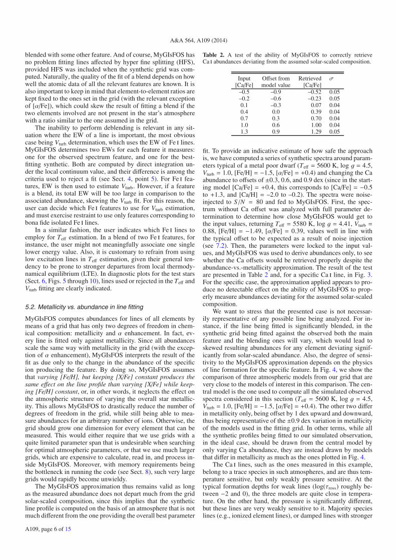
Table 2. A test of the ability of MyGIsFOS to correctly retrieveCa i abundances deviating from the assumed solar-scaled composition.

Input Offset from Retrieved σ[Ca/Fe] model value [Ca/Fe]

–0.5 –0.9 –0.52 0.05–0.2 –0.6 –0.23 0.050.1 –0.3 0.07 0.040.4 0.0 0.39 0.040.7 0.3 0.70 0.041.0 0.6 1.00 0.041.3 0.9 1.29 0.05

fit. To provide an indicative estimate of how safe the approachis, we have computed a series of synthetic spectra around param-eters typical of a metal poor dwarf (Teff = 5600 K, log g = 4.5,Vturb = 1.0, [Fe/H] = −1.5, [α/Fe] = +0.4) and changing the Caabundance to offsets of ±0.3, 0.6, and 0.9 dex (since in the start-ing model [Ca/Fe] = +0.4, this corresponds to [Ca/Fe] = −0.5to +1.3, and [Ca/H] = –2.0 to –0.2). The spectra were noise-injected to S /N = 80 and fed to MyGIsFOS. First, the spec-trum without Ca offset was analyzed with full parameter de-termination to determine how close MyGIsFOS would get tothe input values, returning Teff = 5580 K, log g = 4.41, Vturb =0.88, [Fe/H] = −1.49, [α/Fe] = 0.39, values well in line withthe typical offset to be expected as a result of noise injection(see 7.2). Then, the parameters were locked to the input val-ues, and MyGIsFOS was used to derive abundances only, to seewhether the Ca offsets would be retrieved properly despite theabundance-vs.-metallicity approximation. The result of the testare presented in Table 2 and, for a specific Ca i line, in Fig. 3.For the specific case, the approximation applied appears to pro-duce no detectable effect on the ability of MyGIsFOS to prop-erly measure abundances deviating for the assumed solar-scaledcomposition.

We want to stress that the presented case is not necessar-ily representative of any possible line being analyzed. For in-stance, if the line being fitted is significantly blended, in thesynthetic grid being fitted against the observed both the mainfeature and the blending ones will vary, which would lead toskewed resulting abundances for any element deviating signif-icantly from solar-scaled abundance. Also, the degree of sensi-tivity to the MyGIsFOS approximation depends on the physicsof line formation for the specific feature. In Fig. 4, we show thecomparison of three atmospheric models from our grid that arevery close to the models of interest in this comparison. The cen-tral model is the one used to compute all the simulated observedspectra considered in this section (Teff = 5600 K, log g = 4.5,Vturb = 1.0, [Fe/H] = −1.5, [α/Fe] = +0.4). The other two differin metallicity only, being offset by 1 dex upward and downward,thus being representative of the ±0.9 dex variation in metallicityof the models used in the fitting grid. In other terms, while allthe synthetic profiles being fitted to our simulated observation,in the ideal case, should be drawn from the central model byonly varying Ca abundance, they are instead drawn by modelsthat differ in metallicity as much as the ones plotted in Fig. 4.

The Ca i lines, such as the ones measured in this example,belong to a trace species in such atmospheres, and are thus tem-perature sensitive, but only weakly pressure sensitive. At thetypical formation depths for weak lines (log(τross) roughly be-tween −2 and 0), the three models are quite close in tempera-ture. On the other hand, the pressure is significantly different,but these lines are very weakly sensitive to it. Majority specieslines (e.g., ionized element lines), or damped lines with stronger

A109, page 6 of 15

L. Sbordone et al.: A code for automatic abundance analysis

Fig. 3. The Ca i 559.19 nm line in the case of the two most extreme off-sets described in Sect. 5.2 and in the no-offset case, with their respectivebest fitting synthetic value (magenta profiles). The magenta horizontallines represent local continuum, one-σ, and three-σ of the local simu-lated noise. [Ca/H] is the input value, [Ca/H]best the best fit value for theline.

pressure sensitivity, are likely to display stronger departures inthis situation. As such, we suggest that users verify the abun-dances derived by MyGIsFOS for species that depart heavilyfrom grid solar-scaled values. However, since significant differ-ences might arise only for species strongly departing from solarabundance ratios, the detection of abundance anomalies throughMyGIsFOS is to be considered robust, and only the exact amountof the abundance departure might be in need of verification.

6. Tests on reference stars

As an assessment of MyGIsFOS performance, in this sectionwe present parameter determination and chemical analysis fora few representative stars. To reproduce typical data characteris-tics, very high S/N, high-resolution spectra of five well-studied

Fig. 4. Comparison of Atlas 12 atmosphere models with Teff = 5600log g = 4.5, Vturb = 1.0, [α/Fe] = +0.4 and [Fe/H] = −2.5 (blue lineand triangles), [Fe/H] = −1.5 (black line), and [Fe/H] = −0.5 (red lineand diamonds). Top to bottom: temperature for the three models, tem-perature difference (red line, [Fe/H] = −0.5 – [Fe/H] = −1.5; blue line,[Fe/H] = −2.5 – [Fe/H] = −1.5), pressure in g cm−2, pressure difference,all plotted vs. τross.

stars have been noise-injected at typical real world values andanalyzed using synthetic grids and feature lists appropriate forthe four main broad spectra type: metal rich dwarf/subgiantstars (the Sun, see Sect. 6.1), metal poor dwarf/subgiants(HD 126681, Sect. 6.3, and HD 140283, Sect. 6.4), metal richgiants (Arcturus, Sect. 6.2), and metal poor giants (HD 26297,Sect. 6.5). Given the coverage provided by the available syn-thetic grid, we performed the analysis has been using rangesroughly corresponding to UVES red 580 nm setting, i.e., twoframes covering 480 to 580 nm, and 580 to 680 nm. For eachstar, Tables 3 and 4 report the final determined parameters, plusdetailed abundances for a few chemical species, along with thenumber of lines used and line-to-line scatter, when more thanone line was measured.

A109, page 7 of 15

A&A 564, A109 (2014)

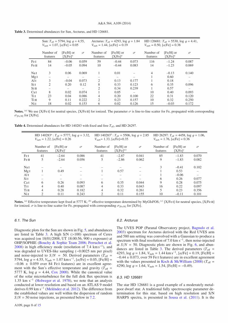
Table 3. Determined abundances for Sun, Arcturus, and HD 126681.

Sun: Teff = 5794, log g = 4.55, Arcturus: Teff = 4293, log g = 1.84 HD 126681: Teff = 5530, log g = 4.41,Vturb = 1.07, [α/Fe] = 0.05 Vturb = 1.44, [α/Fe] = 0.19 Vturb = 0.50, [α/Fe] = 0.38

Number of [Fe/H] or σ Number of [Fe/H] or σ Number of [Fe/H] or σfeatures [X/Fe]a features [X/Fe]a features [X/Fe]a

Fe i 84 –0.06 0.059 59 –0.44 0.073 116 –1.24 0.087Fe ii 14 –0.05 0.094 10 –0.44 0.083 14 –1.23 0.069

Na i 3 0.06 0.069 1 0.01 – 4 –0.13 0.140Mg i – – – – – – 1 0.60 –Al i 3 –0.04 0.073 2 0.13 0.177 1 0.18 –Si i 2 0.20 0.12 8 0.33 0.123 6 0.35 0.096Si ii – – – 2 0.34 0.239 1 0.57 –Ca i 8 0.02 0.074 1 0.05 – 10 0.40 0.093Ti i 23 0.04 0.086 4 0.20 0.100 22 0.31 0.120Ti ii 9 0.11 0.222 2 0.23 0.157 10 0.32 0.250Ni i 18 0.02 0.153 6 0.02 0.126 15 –0.03 0.172

Notes. (a) We use [X/Fe i] for neutral species, [X/Fe ii] for ionized. The parameter σ is line-to-line scatter for Fe, propagated with correspondingσ[Fe/H] for [X/Fe].

Table 4. Determined abundances for HD 140283 with fixed and free Teff , and HD 26297.

HD 140283a : Teff = 5777, log g = 3.32, HD 140283b : Teff = 5506, log g = 2.85 HD 26297: Teff = 4458, log g = 1.06,Vturb = 1.22, [α/Fe] = 0.26 Vturb= 1.33, [α/Fe]=0.35 Vturb = 1.76, [α/Fe] = 0.36

Number of [Fe/H] or σ Number of [Fe/H] or σ Number of [Fe/H] or σfeatures [X/Fe]c features [X/Fe](c) features [X/Fe]c

Fe i 41 –2.64 0.086 41 –2.87 0.041 85 –1.83 0.070Fe ii 5 –2.64 0.056 5 –2.86 0.062 9 –1.83 0.082

Na i – – – – – – 3 –0.41 0.102Mg i 1 0.49 – 1 0.57 – 1 0.53 –Al i – – – – – – 1 –0.06 –Si i – – – – – – 6 0.26 0.077Ca i 6 0.26 0.093 6 0.35 0.044 9 0.28 0.075Ti i 4 0.40 0.087 4 0.33 0.043 16 0.22 0.097Ti ii 4 0.28 0.182 4 0.32 0.261 5 0.23 0.356Ni i 2 0.11 0.243 2 0.11 0.155 10 –0.11 0.101

Notes. (a) Effective temperature kept fixed at 5777 K; (b) effective temperature determined by MyGIsFOS; (c) [X/Fe i] for neutral species, [X/Fe ii]for ionized. σ is line-to-line scatter for Fe, propagated with corresponding σ[Fe/H] for [X/Fe].

6.1. The Sun

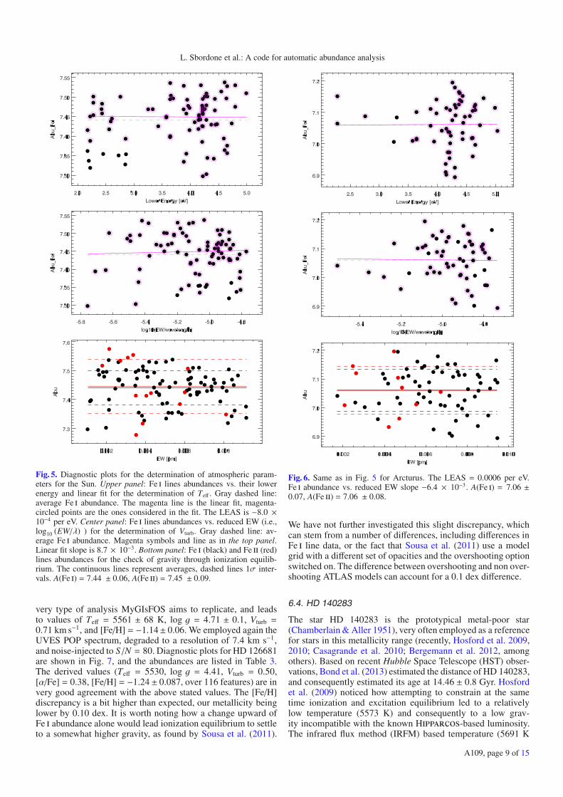
Diagnostic plots for the Sun are shown in Fig. 5, and abundancesare listed in Table 3. A high S/N (>100) spectrum of Cereswas acquired (on 18/01/2008, UT 18:00:56, 900 s exposure) atOHP/SOPHIE (Bouchy & Sophie Team 2006; Perruchot et al.2008) in high efficiency mode (resolution of 7.4 km s−1), andwas degraded to UVES-like sampling (∼0.0025 nm per pixel)and noise-injected to S /N = 50. Derived parameters (Teff =5794, log g = 4.55, Vturb = 1.07 km s−1, [α/Fe] = 0.05, [Fe/H] =−0.06 ± 0.059 over 84 Fe i features) are in excellent agree-ment with the Sun’s effective temperature and gravity (Teff =5777 K, log g = 4.44, Cox 2000). While the canonical valueof the solar microturbulence for the full disk flux spectrum is1.35 km s−1 (Holweger et al. 1978), we note that an analysisconducted at lower resolution and based on an ATLAS 9 modelderives 0.99 km s−1 (Meléndez et al. 2012). The difference fromthe established values are well within the dispersion of randomS /N = 50 noise injections, as presented below in 7.2.

6.2. Arcturus

The UVES POP (Paranal Observatory project, Bagnulo et al.2003) spectrum for Arcturus derived with the Red UVES armand 580 nm setting was convolved with a Gaussian to produce aspectrum with final resolution of 7.0 km s−1, then noise-injectedat S /N = 50. Diagnostic plots are shown in Fig. 6, and abun-dances are listed in Table 3. The derived parameters (Teff =4293, log g = 1.84, Vturb = 1.44 km s−1, [α/Fe] = 0.19, [Fe/H] =−0.44 ± 0.073, over 59 Fe i features) are in excellent agreementwith the values presented in Koch & McWilliam (2008) (Teff =4290, log g = 1.64, Vturb = 1.54, [Fe/H] = −0.49).

6.3. HD 126681

The star HD 126681 is a good example of a moderately metal-poor dwarf star. A traditional fully spectroscopic parameter de-termination for this star, based on high resolution and S/NHARPS spectra, is presented in Sousa et al. (2011). It is the

A109, page 8 of 15

L. Sbordone et al.: A code for automatic abundance analysis

Fig. 5. Diagnostic plots for the determination of atmospheric param-eters for the Sun. Upper panel: Fe i lines abundances vs. their lowerenergy and linear fit for the determination of Teff . Gray dashed line:average Fe i abundance. The magenta line is the linear fit, magenta-circled points are the ones considered in the fit. The LEAS is −8.0 ×10−4 per eV. Center panel: Fe i lines abundances vs. reduced EW (i.e.,log10 (EW/λ) ) for the determination of Vturb. Gray dashed line: av-erage Fe i abundance. Magenta symbols and line as in the top panel.Linear fit slope is 8.7 × 10−3. Bottom panel: Fe i (black) and Fe ii (red)lines abundances for the check of gravity through ionization equilib-rium. The continuous lines represent averages, dashed lines 1σ inter-vals. A(Fe i) = 7.44 ± 0.06, A(Fe ii) = 7.45 ± 0.09.

very type of analysis MyGIsFOS aims to replicate, and leadsto values of Teff = 5561 ± 68 K, log g = 4.71 ± 0.1, Vturb =0.71 km s−1, and [Fe/H] = −1.14± 0.06. We employed again theUVES POP spectrum, degraded to a resolution of 7.4 km s−1,and noise-injected to S /N = 80. Diagnostic plots for HD 126681are shown in Fig. 7, and the abundances are listed in Table 3.The derived values (Teff = 5530, log g = 4.41, Vturb = 0.50,[α/Fe] = 0.38, [Fe/H] = −1.24± 0.087, over 116 features) are invery good agreement with the above stated values. The [Fe/H]discrepancy is a bit higher than expected, our metallicity beinglower by 0.10 dex. It is worth noting how a change upward ofFe i abundance alone would lead ionization equilibrium to settleto a somewhat higher gravity, as found by Sousa et al. (2011).

Fig. 6. Same as in Fig. 5 for Arcturus. The LEAS = 0.0006 per eV.Fe i abundance vs. reduced EW slope −6.4 × 10−3. A(Fe i) = 7.06 ±0.07, A(Fe ii) = 7.06 ± 0.08.

We have not further investigated this slight discrepancy, whichcan stem from a number of differences, including differences inFe i line data, or the fact that Sousa et al. (2011) use a modelgrid with a different set of opacities and the overshooting optionswitched on. The difference between overshooting and non over-shooting ATLAS models can account for a 0.1 dex difference.

6.4. HD 140283

The star HD 140283 is the prototypical metal-poor star(Chamberlain & Aller 1951), very often employed as a referencefor stars in this metallicity range (recently, Hosford et al. 2009,2010; Casagrande et al. 2010; Bergemann et al. 2012, amongothers). Based on recent Hubble Space Telescope (HST) obser-vations, Bond et al. (2013) estimated the distance of HD 140283,and consequently estimated its age at 14.46 ± 0.8 Gyr. Hosfordet al. (2009) noticed how attempting to constrain at the sametime ionization and excitation equilibrium led to a relativelylow temperature (5573 K) and consequently to a low grav-ity incompatible with the known Hipparcos-based luminosity.The infrared flux method (IRFM) based temperature (5691 K

A109, page 9 of 15

A&A 564, A109 (2014)

Fig. 7. Same as in Fig. 5 for HD 126681. LEAS = −0.0002 per eV. Fe iabundance vs. reduced EW slope 8.0 × 10−4. A(Fe i) = 6.26 ± 0.09,A(Fe ii) = 6.27 ± 0.07.

Alonso et al. 1996; 5755 K González Hernández & Bonifacio2009; 5777 K Casagrande et al. 2010) delivers a more satis-factory ionization equilibrium when gravity is derived from theHipparcos luminosity, but this is at the expense of inducing asizeable LEAS (see Tables 2, 3, and Fig. 11 in Bergemann et al.2012). According to Hosford et al. (2010), treating the line trans-fer for Fe i lines in NLTE solves this discrepancy and provides anexcitation temperature of 5838 K, in reasonable agreement withthe IRFM temperatures. Bergemann et al. (2012) disagree withthis finding. What is relevant in the present context is that solv-ing for both excitation and ionization equilibria of iron in LTEfor HD 140283 leads to low temperature and gravity; Hosfordet al. (2009) and Bergemann et al. (2012) agree with this issue.

We employed the UVES POP red arm 580 nm spectra, with-out adding instrumental broadening or injecting noise: due to thehigh resolution of the spectra, stellar rotation and macroturbu-lence might require a broadening of the grid above what is nec-essary to take the instrumental resolution into account. We ad-justed the grid broadening until we obtained satisfactory fits onseveral isolated lines. The final grid broadening employed was5.5 km s−1. We ran MyGIsFOS on this star twice, once leaving

Fig. 8. Same as in Fig. 5 for HD 140283 with the temperature locked atTeff = 5777 K. LEAS = −0.0534 per eV. The Fe i abundance vs. reducedEW slope is 2.3 × 10−3. A(Fe i) = 4.86 ± 0.09, A(Fe ii) = 4.86 ± 0.06.

the code free to constrain all the parameters, and once lockingTeff to 5777 K. Diagnostic plots for HD 140283 are shown inFigs. 8 and 9, and the abundances are listed in Table 4. Whenleaving MyGIsFOS free to set Teff, it falls to 5506 K, reason-ably close to the excitation temperature found by Hosford et al.(2009) also driving down [Fe/H] to −2.87, and log g to 2.86.When fixing Teff at 5777 K, instead, the derived gravity (3.32)is in reasonable agreement with the Hipparcos value (3.73),and Vturb is also very close to the value derived in Bergemannet al. (2012) in the LTE case (1.22 km s−1 vs. 1.27). However,we derive a metallicity lower by about 0.22 dex ([Fe/H] = −2.64vs. −2.42).

6.5. HD 26297

The star HD 26297 is a moderately metal-poor giant star. A spec-troscopic abundance analysis similar to the one MyGIsFOS per-forms is presented in Fulbright (2000) (Teff = 4500 K, log g =1.2, [Fe/H] = −1.72), while Gratton et al. (2000) obtain sim-ilar values (Teff = 4450 K, log g = 1.18, [Fe/H] = −1.68,

A109, page 10 of 15

L. Sbordone et al.: A code for automatic abundance analysis

Fig. 9. Same as in Fig. 5 for HD 140283 with temperature iterated.LEAS = −0.0008 per eV. The Fe i abundance vs. reduced EW slopeis 4.3 × 10−3. A(Fe i) = 4.63 ± 0.04, A(Fe ii) = 4.64 ± 0.06.

Vturb = 1.62 km s−1) but derive temperature and gravity fromphotometric calibrations (Fe ionization equilibrium is very wellsatisfied for this star). A more recent analysis, presented inPrugniel et al. (2011), uses a χ2 minimization algorithm insteadto fit the target spectrum against the empirical ELODIE library(see Wu et al. 2011), and delivers Teff = 4479 K, log g = 1.05,[Fe/H] = −1.78.

We downloaded archival UVES red 580 spectra forHD 26297 (taken on 20/11/2004, 01:39:42 UT, prog. id 074.B-0639). The data were taken with slit width of 0.9′′ and havea good S/N (>100). No additional noise was injected. Theywere analyzed by broadening the synthetic grid to 7.5 km s−1.Diagnostic plots are shown in Fig. 10, and the abundances arelisted in Table 4. We derive Teff = 4458, log g = 1.06, Vturb =1.76, [α/Fe] = 0.36, [Fe/H] = −1.83± 0.07, over 83 Fe i lines, inexcellent agreement with all the cited sources.

7. Monte Carlo simulations

One attractive possibility opened by fully automated abundanceanalysis codes such as MyGIsFOS is to comprehensively assess

Fig. 10. Same as in Fig. 5 for HD 26297. LEAS = 0.0009 per eV. TheFe i abundance vs. reduced EW slope is −5.6 × 10−3. A(Fe i) = 5.67 ±0.07, A(Fe ii) = 5.67 ± 0.08.

the error budget by means of Monte Carlo simulations, sincelarge number of test events can be processed through the code invery little time.

7.1. Impact of S/N: internal errors

To assess the size of MyGIsFOS internal errors, as well as theextent to which the code is affected by spectrum noise, we em-ployed a synthetic spectrum extracted from the MPD grid atTeff = 5400 K, log g = 4.5, Vturb = 1.0 km s−1, [Fe/H] = −1.0,[α/Fe] = +0.4, and processed it to MyGIsFOS after broadening itto a resolution of 7.4 km s−1, and resampling it to typical UVESpixel size. We first processed it without injecting noise to ensurethe absence of systematics, and subsequently produced 1000 in-dependent Poisson noise realizations at S /N = 80, 50, 20, for atotal of 3000 noise realizations, which were fed to MyGIsFOS,set to derive Teff , log g, Vturb, [Fe/H], and [α/Fe]. The results ofthe noiseless test, as well as derived average values and 1σ dis-persions for the noise-injection Monte Carlo tests are listed inTable 5.

A109, page 11 of 15

A&A 564, A109 (2014)

Table 5. Average parameter values and 1σ intervals for the Monte Carlo tests described in Sect. 7.

Test type Teff σ log g σ [Fe/H] σ Vturb σK cm s−1 km s−1

Synthetic noiseless 5403 – 4.51 – –1.00 – 0.97 –

Synthetic S /N = 80 5409 31 4.51 0.06 –1.01 0.02 1.05 0.07Synthetic S /N = 50 5419 36 4.54 0.08 –1.00 0.03 1.04 0.09Synthetic S /N = 20 5461 80 4.57 0.18 –0.95 0.06 0.94 0.22

HD 126681 S /N = 80 5536 36 4.42 0.07 –1.24 0.03 0.58 0.16HD 126681 S /N = 50 5499 46 4.34 0.10 –1.24 0.03 0.47 0.19HD 126681 S /N = 20 5422 87 4.10 0.20 –1.22 0.07 0.39 0.28HD 126681 fixed Teff , S /N = 80 5552 150 4.43 0.29 –1.24 0.12 0.77 0.22

Notes. In order, the result of the analysis of the noiseless synthetic spectrum, of the three 1000 noise realization runs on the synthetic (for both see7.1), of the three 1000 noise realization runs on HD 126681, and of the “photometric Teff” run on HD 126681 (for both see 7.2). In the last row,Teff and its σ are in boldface to indicate they are not results, but the fixed input Teff distribution.

Fig. 11. Histograms of MyGIsFOS parameter determination output in aMonte Carlo simulation of 1000-events noise injection at S /N = 80 ona spectrum of HD 126681. Top to bottom: determined Teff (mean and σ,continuous and dashed red lines, respectively, all values in Table 5),log g, [Fe/H], Vturb.

It is worth noticing how the errors displayed by MyGIsFOSin the synthetic test closely match the ones in the case ofHD126681. One might have expected that feeding MyGIsFOSa spectrum of the same grid used for the analysis would have ledto the code snapping on the right parameters, leading to lower-than-realistic errors. However, MyGIsFOS only compares thegrid and the observed spectrum on a line-by-line basis, and pa-rameters are all derived by indirect methods. Moreover, the ini-tial temperature scan is purposefully performed at steps differentfrom the grid step, so that the comparison is always performedaway from gridpoints, removing any grid snapping effect.

7.2. Impact of S/N: HD 126681

To assess the impact of external error sources we have re-peated the above described test on the very high S/N spectrumof HD126681 described in Sect. 6.3. Again, 1000 independentPoisson noise realizations were produced for S /N = 80, 50,20 each. Derived average values and 1σ dispersions are listedin Table 5, the histograms of the parameters are presented inFigs. 11 through 13.

MyGIsFOS is not allowed to try to bring stellar parametersto convergence indefinitely. After a set number of cycles it stops,declares the star non-converging and moves on to the next one. Itis worth noticing here that, while S /N = 80 and 50 Monte Carlotests had every single star reaching satisfactory convergence, inthe S /N = 20 case convergence was reached in 943 over 1000 re-alizations (a failure rate of 5.7%). Unsurprisingly, at such lowS/N the difficulty of measuring weak lines, needed especiallyfor Vturb determination, begins to take its toll. Moreover, Vturb isestimated at 0 km s−1 for 138 converging stars, a clearly visiblepeak in Fig. 13. This is just the natural consequence of a Vturb dis-tribution centered at 0.39 km s−1 with a σ of 0.28: in a relevantnumber of stars the specific set of Fe i lines used would push fora negative Vturb, which MyGIsFOS forbids as unphysical.

The presented test is a simplified one and the resulting un-certainties are possibly somewhat underestimated. In particular,the injection of Poisson noise is a somewhat optimistic way tosimulate real observed spectrum noise degradation, since it lacksa number of realistic outstanding defects real, low S/N spectrapresent (cosmic ray hits, poor order tracing in low S/N cases,increased noise at order merging points...). Also, noise was in-jected here to produce constant S/N through the range, which isnot the case in practice, often with lower S/N in the bluer part ofthe range, where most of the atomic lines are concentrated.

A109, page 12 of 15

L. Sbordone et al.: A code for automatic abundance analysis

Fig. 12. As in Fig. 11 but now with S /N = 50.

7.3. Impact of predetermined parameters: photometric Teff

Most abundance analysis works typically assess the impact oferrors on atmospheric parameters on derived abundances by as-suming said errors are independent. This is often performed bypicking a representative star in the sample, and repeating theabundance determination by varying one parameter at a timeby an amount considered to be the typical uncertainty on thatparameter. This quick way of estimating parameter uncertaintiesis, however, conceptually flawed in the sense that atmosphericparameters correlate in a fashion that is, ultimately, dependenton the specific way they are derived. For instance, if gravity isdetermined from Fe i-Fe ii ionization equilibrium, varying Teffby 150 K will lead to a different gravity too: repeating the anal-ysis with a different temperature but the same gravity will not be

Fig. 13. As in Fig. 11, but now with S /N = 20.

representative of which effect a 150 K Teff error would have in areal world case.

A fairly common case in which such issue is of importanceis the one in which effective temperatures are derived indepen-dently from the spectra, e.g., from photometry. In this case, er-rors in the other parameters cascade from whatever error is madein Teff , in a systematic way. MyGIsFOS allows us to estimatethe effect through a Monte Carlo test set. We again constructeda 1000-events test set but, in contrast to what we did in 7.2, wehave now analyzed one single realization of S /N = 80 noiseinjection, starting from the same HD 126681 high-S/N spec-trum. We now constructed the test set by drawing 1000Teff val-ues from a Gaussian distribution centered at 5552 K and with a σof 150 K, and having MyGIsFOS run with fixed Teff. The result-ing histograms are shown in Fig. 14, the resulting distributions in

A109, page 13 of 15

A&A 564, A109 (2014)

Fig. 14. Histograms of MyGIsFOS parameter determination output ina 1000-events Monte Carlo simulation with fixed Teff , on a S /N = 80spectrum of HD 126681. Panels as in Fig. 11.

the other parameters and metallicity are again listed in Table 5.Although we do not present it here, a more detailed species-by-species error estimate is of course possible, thus allowingto properly assess parameter-related uncertainties on any abun-dance. The same kind of procedure is, of course, possible whenmore than one parameter is kept fixed (e.g., the case of photo-metric Teff and log g derived from isochrones).

8. Performance, system requirements,and availability

MyGIsFOS is written in Fortran 90 with Intel extensions. Sofar it has been compiled and run under Linux and Mac OS X.

MyGIsFOS synthetic grids can grow to significant sizes whencovering large spectral ranges and a large parameter space. Asan example, we consider the grid employed in Sects. 6.3, 6.4,and 7, intended to handle UVES RED 580 spectra of metal poor,cool turn off and dwarf stars. It is composed of two frames (460to 590, and 560 to 690 nm) synthesized (from ATLAS12 atmo-sphere models and by using SYNTHE, see Sbordone et al. 2004;Castelli 2005; Kurucz 2005; Sbordone 2005) with velocity-equispaced, R = 300 000 sampling. The spectra are computedfor 3840 parameter values5. The binary packaged grid has a sizeof about 2.2 GB. The size of the grid sets the main resourcerequirement, since the grid is twice resident in memory (themaster copy read in at the beginning of the run, and the one,smaller, resampled to the observed pixels of the star being cur-rently processed). Also, grid resampling at observed spectrumpixel wavelengths is usually the longest operation in the pro-cessing of a star. For both these reasons, it is always advisable touse the smallest desirable grid both in terms of parameter spaceand spectrum coverage.

As a benchmarking and resource consumption reference, weuse typical values for one of the S/N Monte Carlo runs describedin Sect. 7.2. The run was executed on a quad-core Intel XeonE31245, 3.3 GHz, machine with 11.6 GB of RAM, runningopenSUSE 12.3 with 3.7.10 64 bit kernel. Employing the griddescribed above in this same section, peak MyGIsFOS mem-ory consumption was 3.5 GB, with an average processing timeper star (over 1000 stars) of 119 s, running on a single core6.These values are to be considered upper limits. In the describedcase, the resampling of ∼74 700 synthetic grid “pixels” over the∼71 000 observed ones takes somewhat more of 50% of the to-tal per-star processing time, almost all the rest being taken bythe ∼280 parameter-finding iterations needed to determine Teff ,log g Vturb, [Fe/H], and [α/Fe]. At the other extreme, determin-ing only [Fe/H], [α/Fe], and detailed abundances at predefinedatmospheric parameters on data constituted by two FLAMEShigh-resolution settings takes less than 10 s per star, thanksequally to the lack of parameter iteration and to the small num-ber of pixels over which grid resampling should be performed.

For the time being, MyGIsFOS is available on a collabora-tion basis only. A website has been set up to make detailed codedocumentation available to interested parties, so that they canassess whether it can be of use to them before contacting us.

9. Conclusions

We have presented MyGIsFOS, an automatic code for the deter-mination of atmospheric parameters and detailed chemical abun-dances in cool stars. Replicating as closely as possible a tradi-tional manual abundance analysis technique for these types ofstars, MyGIsFOS derives results directly and quickly compara-ble with well-known analysis techniques. Currently, MyGIsFOShas been employed on the same type of data that are best suitedfor the manual techniques it replicates, i.e., those character-ized by high-resolution and/or broad spectral coverage, such asthe ones delivered by UVES, X-shooter (Vernet et al. 2011),

5 Listing start, end, step, and number of steps. Teff[K]: 5000, 6000,200, 6; log g[cm s−1]: 3.0, 5.0, 0.5, 5; Vturb[km s−1]: 0.0, 3.0, 1.0, 4;[Fe/H]: −4.0, −0.5, 0.5, 8; [α/Fe]: −0.4, 0.8, 0.4, 4.6 MyGIsFOSis not currently written or compiled to use more than onethread. This would surely speed up the execution significantly, but wedo not see it as a priority, since the code is already fast enough that theactual bottleneck is the “human time” to prepare the input and checkthe results, rather than the processor time.

A109, page 14 of 15

L. Sbordone et al.: A code for automatic abundance analysis

HARPS, Sophie (Caffau et al. 2011a; Bonifacio et al. 2012;Caffau et al. 2012, 2013; Duffau et al., in prep.). Its very fastoperation (two minutes or less per star on a mainstream personalcomputer) is useful in a number of circumstances. For instance,it is convenient when analyzing large datasets of (broadly) ho-mogeneous data in the context of large scale spectroscopic sur-veys, for instance, the Gaia-ESO Public Survey (UVES data,see Gilmore et al. 2012). It can also be used when screeninglarge amounts of low-intermediate resolution spectra for inter-esting candidates to be followed up. While MyGIsFOS deliversits full capability for high-resolution (R ≥ 25 000), large spectralcoverage data, it can be effectively used to derive global metal-licity from low-resolution spectra, once parameters can be in-ferred from other sources. In this context Abbo (Bonifacio &Caffau 2003), the code MyGIsFOS has been derived from, hasbeen employed to select extremely metal poor turn off candidatesfrom low-resolution SDSS-SEGUE (York et al. 2000; Yannyet al. 2009) spectra, which were then followed up at high resolu-tion, showing a remarkable selection success rate (e.g., Caffauet al. 2012; Bonifacio et al. 2012; Caffau et al. 2011a), andMyGIsFOS is currently used in the same capacity in the contextof the TOPoS ESO Large Program (Turn-Off Primordial Stars,Caffau et al. 2013). It can also be very useful to extend preexist-ing literature datasets with new data: when adding new stars topre-existing samples of abundances derived in previous papers,it is usually impractical to reanalize the existing corpus of data,so homogeneity issues arise because of differences, e.g., in atmo-sphere modeling, or atomic data choices. The very fast process-ing of MyGIsFOS permits, on the other hand, repeated analysisof the whole sample in a fully homogeneous way every time.As a matter of fact, fully parallel analyses can be conducted,e. g., with different atmospheric parameter choices, with prac-tically no time penalty. Also, MyGIsFOS allows to consistentlytackle error propagation through the analysis pipeline by meansof Monte Carlo simulations, as presented in Sect. 7.3 for pho-tometric effective temperatures. This is almost never done dueto the very high time cost it would usually imply, but it wouldbe of great importance since errors in atmospheric parametersand abundances are, in general, strongly correlated, and methoddependent.

Acknowledgements. L.S., E.C., and S.D. aknowledge the support ofSonderforschungsbereich SFB 881 “The Milky Way System” (subprojectsA4 and A5) of the German Research Foundation (DFG). P.B. acknowledgessupport from the Conseil Scientifique de l’Observatoire de Paris and from theProgramme National de Cosmologie et Galaxies of the Institut National desSciences de l’Univers of CNRS. This research has made use of the SIMBADdatabase, operated at CDS, Strasbourg, France, and of NASA’s AstrophysicsData System, and is partly based on data obtained from the ESO ScienceArchive Facility.

ReferencesAllende Prieto, C. 2004, Astron. Nachr., 325, 604Allende Prieto, C., Rebolo, R., García López, R. J., et al. 2000, AJ, 120, 1516Allende Prieto, C., Sivarani, T., Beers, T. C., et al. 2008, AJ, 136, 2070Alonso, A., Arribas, S., & Martinez-Roger, C. 1996, A&AS, 117, 227

Bagnulo, S., Jehin, E., Ledoux, C., et al. 2003, The Messenger, 114, 10Bailer-Jones, C. A. L. 2000, A&A, 357, 197Barklem, P. S., Christlieb, N., Beers, T. C., et al. 2005, A&A, 439, 129Bergemann, M., Lind, K., Collet, R., Magic, Z., & Asplund, M. 2012, MNRAS,

427, 27Boeche, C., Siebert, A., Williams, M., et al. 2011, AJ, 142, 193Bond, H. E., Nelan, E. P., VandenBerg, D. A., Schaefer, G. H., & Harmer, D.

2013, ApJ, 765, L12Bonifacio, P. 2005, Mem. Soc. Astron. It. Suppl., 8, 114Bonifacio, P., & Caffau, E. 2003, A&A, 399, 1183Bonifacio, P., Sbordone, L., Caffau, E., et al. 2012, A&A, 542, A87Bouchy, F., & Sophie Team 2006, in Tenth Anniversary of 51 Peg-b: Status of

and prospects for hot Jupiter studies (Paris: Frontier Group), 319Caffau, E., Bonifacio, P., François, P., et al. 2011a, Nature, 477, 67Caffau, E., Ludwig, H.-G., Steffen, M., Freytag, B., & Bonifacio, P. 2011b,

Sol. Phys., 268, 255Caffau, E., Bonifacio, P., François, P., et al. 2012, A&A, 542, A51Caffau, E., Bonifacio, P., Sbordone, L., et al. 2013, A&A, 560, A71Casagrande, L., Ramírez, I., Meléndez, J., Bessell, M., & Asplund, M. 2010,

A&A, 512, A54Castelli, F. 2005, Mem. Soc. Astron. It. Suppl., 8, 25Chamberlain, J. W., & Aller, L. H. 1951, ApJ, 114, 52Cox, A. N. 2000, Allen’s Astrophysical Quantities (Springer)Dekker, H., D’Odorico, S., Kaufer, A., Delabre, B., & Kotzlowski, H. 2000,

Proc. SPIE, 4008, 534Erspamer, D., & North, P. 2002, A&A, 383, 227François, P., Depagne, E., Hill, V., et al. 2003, A&A, 403, 1105Fulbright, J. P. 2000, AJ, 120, 1841Gilmore, G., Randich, S., Asplund, M., et al. 2012, The Messenger, 147, 25González Hernández, J. I., & Bonifacio, P. 2009, A&A, 497, 497Gratton, R. G., Sneden, C., Carretta, E., & Bragaglia, A. 2000, A&A, 354, 169Holweger, H., Gehlsen, M., & Ruland, F. 1978, A&A, 70, 537Hosford, A., Ryan, S. G., García Pérez, A. E., Norris, J. E., & Olive, K. A. 2009,

A&A, 493, 601Hosford, A., García Pérez, A. E., Collet, R., et al. 2010, A&A, 511, A47Katz, D., Soubiran, C., Cayrel, R., Adda, M., & Cautain, R. 1998, A&A, 338,

151Koch, A., & McWilliam, A. 2008, AJ, 135, 1551Kurucz, R. L. 2005, Mem. Soc. Astron. It. Suppl., 8, 14Lodders, K., Plame, H., & Gail, H.-P. 2009, Landolt-Börnstein – Group VI

Astronomy and Astrophysics Numerical Data and Functional Relationshipsin Science and Technology, Solar System, ed. J. E. Trümper, 4, 44

Meléndez, J., Bergemann, M., Cohen, J. G., et al. 2012, A&A, 543, A29Magrini, L., Randich, S., Friel, E., et al. 2013, A&A, 558, A38Mucciarelli, A., Pancino, E., Lovisi, L., Ferraro, F. R., & Lapenna, E. 2013, ApJ,

766, 78Pasquini, L., Avila, G., Blecha, A., et al. 2002, The Messenger, 110, 1Perruchot, S., Kohler, D., Bouchy, F., et al. 2008, Proc. SPIE, 7014,Posbic, H., Katz, D., Caffau, E., et al. 2012, A&A, 544, A154Prugniel, P., Vauglin, I., & Koleva, M. 2011, A&A, 531, A165Recio-Blanco, A., Bijaoui, A., & de Laverny, P. 2006, MNRAS, 370, 141Sbordone, L. 2005, Mem. Soc. Astron. It. Suppl., 8, 61Sbordone, L., Bonifacio, P., Castelli, F., & Kurucz, R. L. 2004, Mem. Soc.

Astron. It. Suppl., 5, 93Sousa, S. G., Santos, N. C., Israelian, G., Mayor, M., & Monteiro, M. J. P. F. G.

2007, A&A, 469, 783Sousa, S. G., Santos, N. C., Israelian, G., Mayor, M., & Udry, S. 2011, A&A,

533, A141Stetson, P. B., & Pancino, E. 2008, PASP, 120, 1332Valenti, J. A., & Piskunov, N. 1996, A&AS, 118, 595Van der Swaelmen, M., Hill, V., Primas, F., & Cole, A. A. 2013, A&A, 560,

A44Vernet, J., Dekker, H., D’Odorico, S., et al. 2011, A&A, 536, A105Wu, Y., Singh, H. P., Prugniel, P., Gupta, R., & Koleva, M. 2011, A&A, 525,

A71Yanny, B., Rockosi, C., Newberg, H. J., et al. 2009, AJ, 137, 4377York, D. G., Adelman, J., Anderson, John, E., Jr., et al. 2000, AJ, 120, 1579

A109, page 15 of 15