ASSAM SCIENCE AND TECHNOLOGY UNIVERSITY

COURSE STRUCTURE

Semester – IV/ Electronics and Communication Engineering/B Tech

Sl.

No.

Sub Code Subject L T P Credit

Theory

1 MA131401 Numerical Methods and Computing 3 2 0 4

2 EC131402 Analog Electronic Circuits 3 2 0 4

3 EC131403 Digital Electronics 3 0 0 3

4 EC131404 Signals and Systems 3 0 0 3

5 EC131405 Random Variables and Stochastic process 3 0 0 3

6 HS131406 Economics and Accountancy 4 0 0 4

Practical

7 MA131411 Numerical Methods and Computation Lab 0 0 2 1

8 EC131412 Analog Electronics Lab 0 0 2 1

8 EC131413 Digital Electronics Lab 0 0 2 1

9 EC131414 Signals and Systems Lab 0 0 2 1

Total 19 4 8 25

Total Contact Hours = 31

Total Credits = 25

Course Title: NUMERICAL METHODS AND COMPUTATION

Course Code: MA131401

L-T-P:C 3-2-0-4

Abstract:

This course is introduced in degree program to identify and classify numerical problems and

also can give an idea about the use of different numerical problems. Different numerical

methods are included here so that one can model (mathematical modelling) practical

problems and can solve using a definite method by seeing mathematical model.

Prerequisites: Mathematics III (MA131301)

Course Outcomes:

Can identify and classify the numerical problem to be solved.

Can choose the most appropriate numerical method for its solution based on

characteristics of the problem.

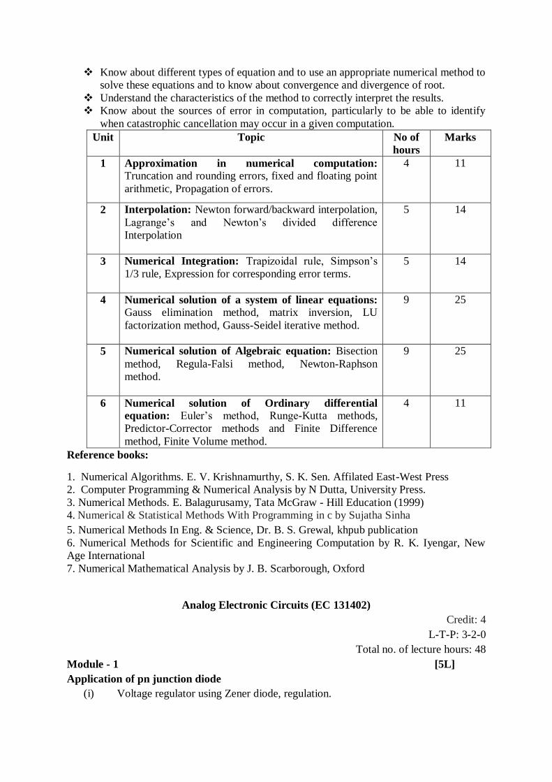
Know about different types of equation and to use an appropriate numerical method to

solve these equations and to know about convergence and divergence of root.

Understand the characteristics of the method to correctly interpret the results.

Know about the sources of error in computation, particularly to be able to identify

when catastrophic cancellation may occur in a given computation.

Unit Topic No of

hours

Marks

1 Approximation in numerical computation:

Truncation and rounding errors, fixed and floating point

arithmetic, Propagation of errors.

4 11

2 Interpolation: Newton forward/backward interpolation,

Lagrange’s and Newton’s divided difference

Interpolation

5 14

3 Numerical Integration: Trapizoidal rule, Simpson’s

1/3 rule, Expression for corresponding error terms.

5 14

4 Numerical solution of a system of linear equations:

Gauss elimination method, matrix inversion, LU

factorization method, Gauss-Seidel iterative method.

9 25

5 Numerical solution of Algebraic equation: Bisection

method, Regula-Falsi method, Newton-Raphson

method.

9 25

6 Numerical solution of Ordinary differential

equation: Euler’s method, Runge-Kutta methods,

Predictor-Corrector methods and Finite Difference

method, Finite Volume method.

4 11

Reference books:

1. Numerical Algorithms. E. V. Krishnamurthy, S. K. Sen. Affilated East-West Press

2. Computer Programming & Numerical Analysis by N Dutta, University Press.

3. Numerical Methods. E. Balagurusamy, Tata McGraw - Hill Education (1999)

4. Numerical & Statistical Methods With Programming in c by Sujatha Sinha

5. Numerical Methods In Eng. & Science, Dr. B. S. Grewal, khpub publication

6. Numerical Methods for Scientific and Engineering Computation by R. K. Iyengar, New

Age International

7. Numerical Mathematical Analysis by J. B. Scarborough, Oxford

Analog Electronic Circuits (EC 131402)

Credit: 4

L-T-P: 3-2-0

Total no. of lecture hours: 48

Module - 1 [5L]

Application of pn junction diode

(i) Voltage regulator using Zener diode, regulation.

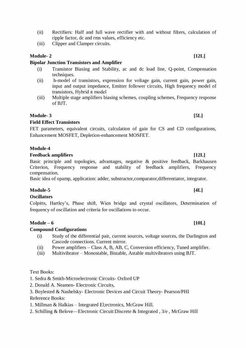
(ii) Rectifiers: Half and full wave rectifier with and without filters, calculation of

ripple factor, dc and rms values, efficiency etc.

(iii) Clipper and Clamper circuits.

Module- 2 [12L]

Bipolar Junction Transistors and Amplifier

(i) Transistor Biasing and Stability, ac and dc load line, Q-point, Compensation

techniques.

(ii) h-model of transistors, expression for voltage gain, current gain, power gain,

input and output impedance, Emitter follower circuits, High frequency model of

transistors, Hybrid π model

(iii) Multiple stage amplifiers biasing schemes, coupling schemes, Frequency response

of BJT.

Module- 3 [5L]

Field Effect Transistors

FET parameters, equivalent circuits, calculation of gain for CS and CD configurations,

Enhancement MOSFET, Depletion-enhancement MOSFET.

Module-4

Feedback amplifiers [12L]

Basic principle and topologies, advantages, negative & positive feedback, Barkhausen

Criterion, Frequency response and stability of feedback amplifiers, Frequency

compensation.

Basic idea of opamp, application: adder, substractor,comparator,differentiator, integrator.

Module-5 [4L]

Oscillators

Colpitts, Hartley’s, Phase shift, Wien bridge and crystal oscillators, Determination of

frequency of oscillation and criteria for oscillations to occur.

Module – 6 [10L]

Compound Configurations

(i) Study of the differential pair, current sources, voltage sources, the Darlington and

Cascode connections. Current mirror.

(ii) Power amplifiers – Class A, B, AB, C, Conversion efficiency, Tuned amplifier.

(iii) Multivibrator – Monostable, Bistable, Astable multivibrators using BJT.

Text Books:

1. Sedra & Smith-Microelectronic Circuits- Oxford UP

2. Donald A. Neamen- Electronic Circuits,

3. Boylested & Nashelsky- Electronic Devices and Circuit Theory- Pearson/PHI

Reference Books:

1. Millman & Halkias – Integrated El;ectronics, McGraw Hill.

2. Schilling & Belove—Electronic Circuit:Discrete & Integrated , 3/e , McGraw Hill

3. Malvino—Electronic Principles , 6/e , McGraw Hill

4. Horowitz & Hill- The Art of Electronics; Cambridge University Press.

DIGITAL ELECTRONICS (EC131403)

Credit: 3

L-T-P: 3-0-0

Total no. of lecture hours: 48

Total lecture hours: 48

UNIT 1 FUNDAMENTALS OF DIGITAL TECHNIQUES:

Lecture hours: 8

Review of Number systems: Positional number systems - decimal, binary, octal and

hexadecimal. Number base conversion.Representation of negative binary numbers. Codes -

BCD, Gray, Excess-3.

Digital signal, logic gates: AND. OR, NOT. NAND. NOR- EX-OR, EX-NOR.

UNIT 2 BOOLEAN ALGEBRA AND ITS SIMPLIFICATION:

Lecture hours: 12

Axioms and basic theorems of Boolean algebra. Truth table, logic functions and their

realization, standard representation (canonical forms) of logic functions - SOP and POS

forms. Min terms and Max terms.

Simplification of logic functions: Karnaugh map of 2, 3, 4 and 5 variables. Simplification by

algebra and by map method. Don’t care condition. Quine Mcluskey methods of

simplification.

Synthesis using AND, OR and INVERT and then to convert to NAND or NOR

implementation.

UNIT 3 COMBINATIONAL LOGIC CIRCUIT DESIGN:

Lecture hours:8

Combinational logic circuits and building blocks. Binary adders and subtractors. Carry look

ahead adder. Encoders, decoders, multiplexers, demultiplexers, comparators, parity

generators etc. Realization of logic functions through decoders and multiplexers.

UNIT 4 SEQUENTIAL CIRCUITS:

Lecture hours:12

Flip Flops: truth table and state table S-R- J-K. T. D, race around condition, master-slave,

conversion of flip flops

Sequential shift registers, sequence generators.

Counters: Asynchronous and Synchronous Ring counters and Johnson Counter, up/down

counter, modulo – N counter. Design of Synchronous sequential circuits.

UNIT 5 DIGITAL LOGIC FAMILIES and PROGRAMMABLE LOGIC DEVICES:

Lecture hours:8

Switching mode operation of p-n junction, bipolar and MOS-devices. Bipolar logic families:

RTL, DTL, DCTL. HTL, TTL, ECL, MOS, and CMOS logic families. Tristate logic.

Gate properties fan-in, fanout, propagation delay and power-delay product.

RAM and ROM - their uses ,SSI, MSI LSI and V LSI devices, Introduction to PLA. PAL to

FPGA and CPLDs. Some commonly used digital ICs.

REFERENCE BOOKS:

1. Modem Digital Electronics (Edition III): R. P. Jain; TMH

2. Digital Integrated Electronics: Taub & Schilling: MGH

3. Digital Principles and Applications: Malvino & Leach: McGraw Hill.

4. Digital Design: Morris Mano: PHI,

5. Digital Electronics-Kharate, Oxford University press

6. Digital Electronics- Salivahanan

7. Fundamentals of digital circuits – Anand Kumar.

8. Digital Electronics: Principle and applications- S. Mandal: TMH

Signals and Systems (EC131404)

Credit: 3 L-T-P: 3-0-0

Total no. of lecture hours: 46

Prerequisite:

I. Five year courses

II. Concepts in electrical and electronic circuits (Basic Electrical and

Electronics Engg. I &II)

III. Knowledge in algebra and calculus

IV. Network Analysis

Hrs

Module 1: Introduction to signals and systems 10

Continuous and discrete time signals, Classification of signals and systems, sum elementary

signals, singularity functions: Unit step, Unit Impulse and Unit Ramp functions. Periodic and

aperiodic signals, Even and odd signals, Causal and non-causal signals. Transformation of

independent variable(time): Time shifting, time scaling, time reversal. Basic system

properties: Linear and non-linear systems, time varying and time invariant systems, Causal

and non-causal systems, Stable and unstable systems.

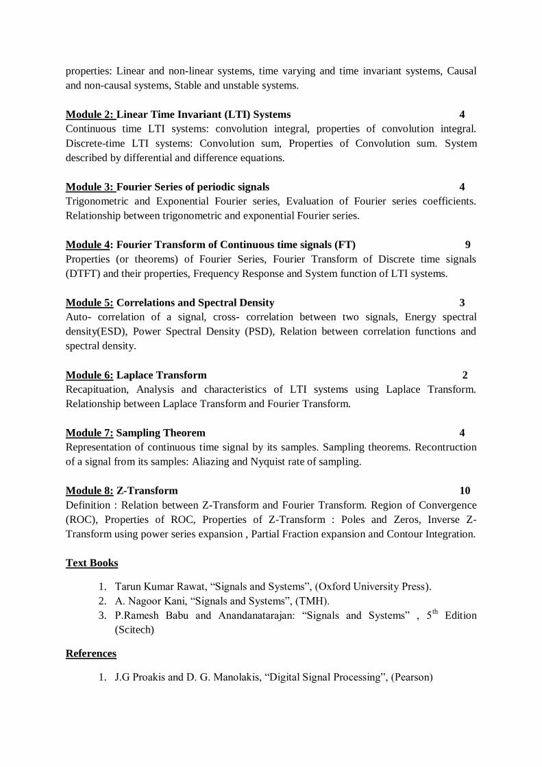
Module 2: Linear Time Invariant (LTI) Systems 4

Continuous time LTI systems: convolution integral, properties of convolution integral.

Discrete-time LTI systems: Convolution sum, Properties of Convolution sum. System

described by differential and difference equations.

Module 3: Fourier Series of periodic signals 4

Trigonometric and Exponential Fourier series, Evaluation of Fourier series coefficients.

Relationship between trigonometric and exponential Fourier series.

Module 4: Fourier Transform of Continuous time signals (FT) 9

Properties (or theorems) of Fourier Series, Fourier Transform of Discrete time signals

(DTFT) and their properties, Frequency Response and System function of LTI systems.

Module 5: Correlations and Spectral Density 3

Auto- correlation of a signal, cross- correlation between two signals, Energy spectral

density(ESD), Power Spectral Density (PSD), Relation between correlation functions and

spectral density.

Module 6: Laplace Transform 2

Recapituation, Analysis and characteristics of LTI systems using Laplace Transform.

Relationship between Laplace Transform and Fourier Transform.

Module 7: Sampling Theorem 4

Representation of continuous time signal by its samples. Sampling theorems. Recontruction

of a signal from its samples: Aliazing and Nyquist rate of sampling.

Module 8: Z-Transform 10

Definition : Relation between Z-Transform and Fourier Transform. Region of Convergence

(ROC), Properties of ROC, Properties of Z-Transform : Poles and Zeros, Inverse Z-

Transform using power series expansion , Partial Fraction expansion and Contour Integration.

Text Books

1. Tarun Kumar Rawat, ―Signals and Systems‖, (Oxford University Press).

2. A. Nagoor Kani, ―Signals and Systems‖, (TMH).

3. P.Ramesh Babu and Anandanatarajan: ―Signals and Systems‖ , 5th Edition

(Scitech)

References

1. J.G Proakis and D. G. Manolakis, ―Digital Signal Processing‖, (Pearson)

2. B.P. Lathi, ―Principles of Linear Systems and Signals‖ , 2e, (Oxford University

Press)

3. M. H. Hayes, ― Digital Signal Processing‖( Schaum’s Outline, TMH)

4. L.F. Chaparro, ―Signals and Systems using MATLAB‖ (Elsevier)

5. Hsu, ―Signals and Systems‖ ( Schaum’s Outline, TMH)

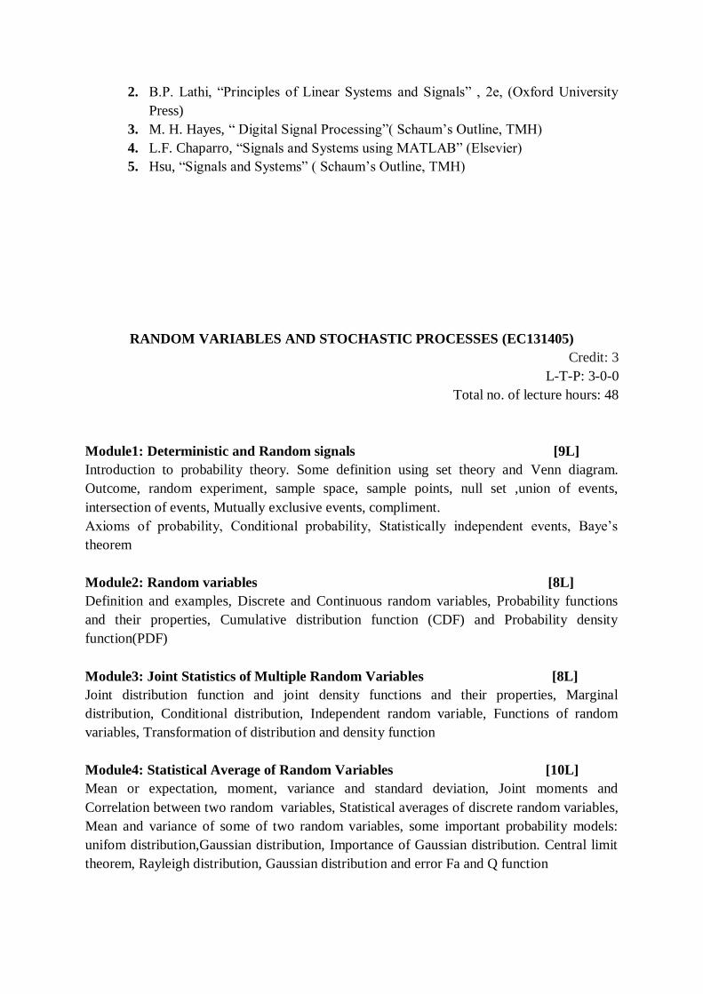
RANDOM VARIABLES AND STOCHASTIC PROCESSES (EC131405)

Credit: 3

L-T-P: 3-0-0

Total no. of lecture hours: 48

Module1: Deterministic and Random signals [9L]

Introduction to probability theory. Some definition using set theory and Venn diagram.

Outcome, random experiment, sample space, sample points, null set ,union of events,

intersection of events, Mutually exclusive events, compliment.

Axioms of probability, Conditional probability, Statistically independent events, Baye’s

theorem

Module2: Random variables [8L]

Definition and examples, Discrete and Continuous random variables, Probability functions

and their properties, Cumulative distribution function (CDF) and Probability density

function(PDF)

Module3: Joint Statistics of Multiple Random Variables [8L]

Joint distribution function and joint density functions and their properties, Marginal

distribution, Conditional distribution, Independent random variable, Functions of random

variables, Transformation of distribution and density function

Module4: Statistical Average of Random Variables [10L]

Mean or expectation, moment, variance and standard deviation, Joint moments and

Correlation between two random variables, Statistical averages of discrete random variables,

Mean and variance of some of two random variables, some important probability models:

unifom distribution,Gaussian distribution, Importance of Gaussian distribution. Central limit

theorem, Rayleigh distribution, Gaussian distribution and error Fa and Q function

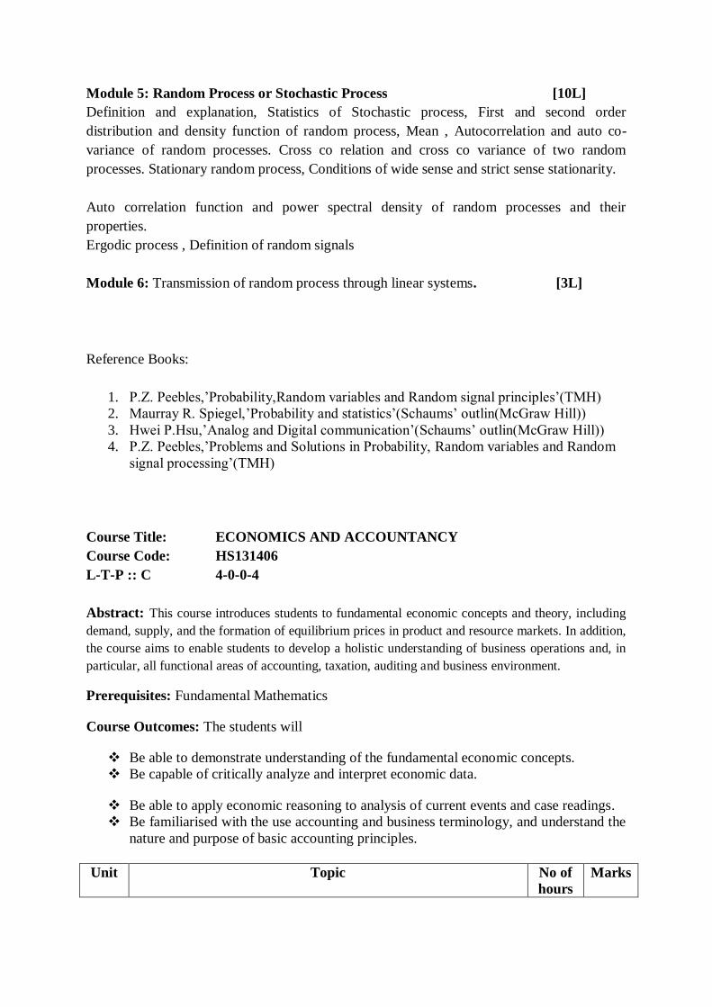
Module 5: Random Process or Stochastic Process [10L]

Definition and explanation, Statistics of Stochastic process, First and second order

distribution and density function of random process, Mean , Autocorrelation and auto co-

variance of random processes. Cross co relation and cross co variance of two random

processes. Stationary random process, Conditions of wide sense and strict sense stationarity.

Auto correlation function and power spectral density of random processes and their

properties.

Ergodic process , Definition of random signals

Module 6: Transmission of random process through linear systems. [3L]

Reference Books:

1. P.Z. Peebles,’Probability,Random variables and Random signal principles’(TMH)

2. Maurray R. Spiegel,’Probability and statistics’(Schaums’ outlin(McGraw Hill))

3. Hwei P.Hsu,’Analog and Digital communication’(Schaums’ outlin(McGraw Hill))

4. P.Z. Peebles,’Problems and Solutions in Probability, Random variables and Random

signal processing’(TMH)

Course Title: ECONOMICS AND ACCOUNTANCY

Course Code: HS131406

L-T-P :: C 4-0-0-4

Abstract: This course introduces students to fundamental economic concepts and theory, including

demand, supply, and the formation of equilibrium prices in product and resource markets. In addition,

the course aims to enable students to develop a holistic understanding of business operations and, in

particular, all functional areas of accounting, taxation, auditing and business environment.

Prerequisites: Fundamental Mathematics

Course Outcomes: The students will

Be able to demonstrate understanding of the fundamental economic concepts.

Be capable of critically analyze and interpret economic data.

Be able to apply economic reasoning to analysis of current events and case readings.

Be familiarised with the use accounting and business terminology, and understand the

nature and purpose of basic accounting principles.

Unit Topic No of

hours

Marks

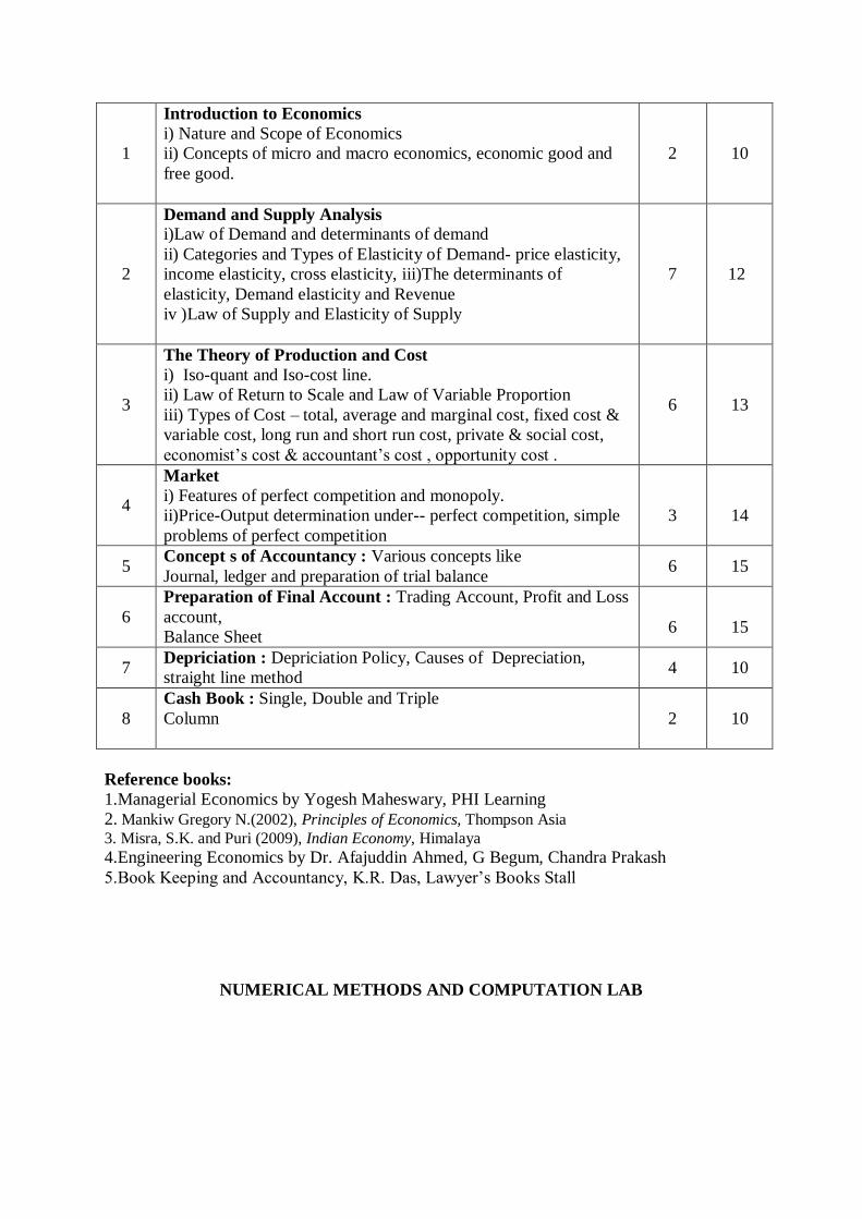
1

Introduction to Economics

i) Nature and Scope of Economics

ii) Concepts of micro and macro economics, economic good and

free good.

2 10

2

Demand and Supply Analysis

i)Law of Demand and determinants of demand

ii) Categories and Types of Elasticity of Demand- price elasticity,

income elasticity, cross elasticity, iii)The determinants of

elasticity, Demand elasticity and Revenue

iv )Law of Supply and Elasticity of Supply

7

12

3

The Theory of Production and Cost

i) Iso-quant and Iso-cost line.

ii) Law of Return to Scale and Law of Variable Proportion

iii) Types of Cost – total, average and marginal cost, fixed cost &

variable cost, long run and short run cost, private & social cost,

economist’s cost & accountant’s cost , opportunity cost .

6

13

4

Market

i) Features of perfect competition and monopoly.

ii)Price-Output determination under-- perfect competition, simple

problems of perfect competition

3

14

5 Concept s of Accountancy : Various concepts like

Journal, ledger and preparation of trial balance 6 15

6

Preparation of Final Account : Trading Account, Profit and Loss

account,

Balance Sheet

6

15

7 Depriciation : Depriciation Policy, Causes of Depreciation,

straight line method 4 10

8

Cash Book : Single, Double and Triple

Column

2

10

Reference books:

1.Managerial Economics by Yogesh Maheswary, PHI Learning

2. Mankiw Gregory N.(2002), Principles of Economics, Thompson Asia

3. Misra, S.K. and Puri (2009), Indian Economy, Himalaya 4.Engineering Economics by Dr. Afajuddin Ahmed, G Begum, Chandra Prakash

5.Book Keeping and Accountancy, K.R. Das, Lawyer’s Books Stall

NUMERICAL METHODS AND COMPUTATION LAB

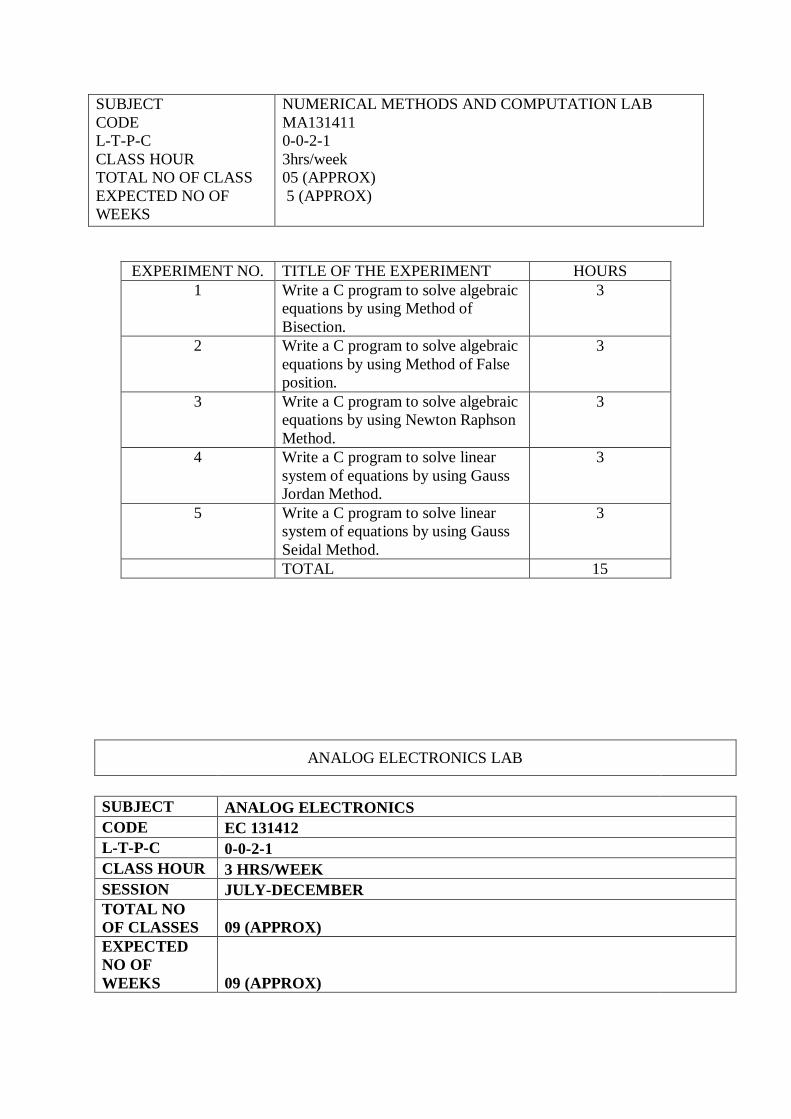
SUBJECT

CODE

L-T-P-C

CLASS HOUR

TOTAL NO OF CLASS

EXPECTED NO OF

WEEKS

NUMERICAL METHODS AND COMPUTATION LAB

MA131411

0-0-2-1

3hrs/week

05 (APPROX)

5 (APPROX)

EXPERIMENT NO. TITLE OF THE EXPERIMENT HOURS

1 Write a C program to solve algebraic

equations by using Method of

Bisection.

3

2 Write a C program to solve algebraic

equations by using Method of False

position.

3

3 Write a C program to solve algebraic

equations by using Newton Raphson

Method.

3

4 Write a C program to solve linear

system of equations by using Gauss

Jordan Method.

3

5 Write a C program to solve linear

system of equations by using Gauss

Seidal Method.

3

TOTAL 15

ANALOG ELECTRONICS LAB

SUBJECT ANALOG ELECTRONICS

CODE EC 131412

L-T-P-C 0-0-2-1

CLASS HOUR 3 HRS/WEEK

SESSION JULY-DECEMBER

TOTAL NO

OF CLASSES 09 (APPROX)

EXPECTED

NO OF

WEEKS 09 (APPROX)

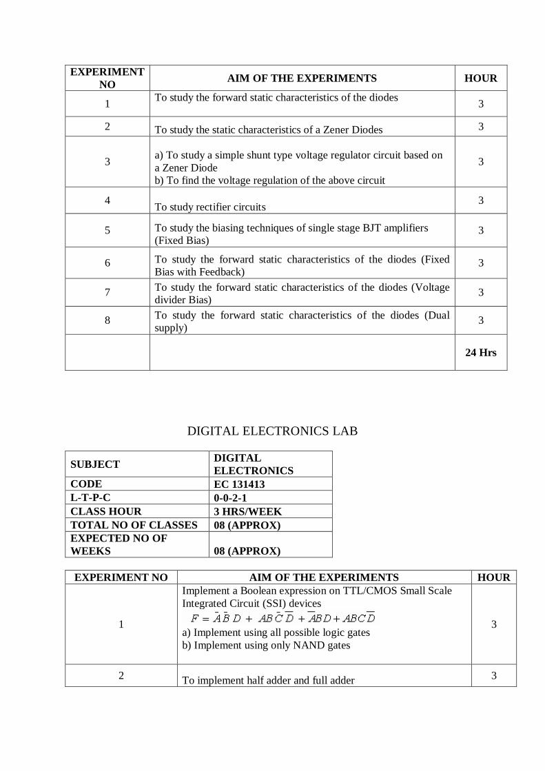
EXPERIMENT

NO AIM OF THE EXPERIMENTS HOUR

1 To study the forward static characteristics of the diodes

3

2 To study the static characteristics of a Zener Diodes 3

3 a) To study a simple shunt type voltage regulator circuit based on

a Zener Diode

b) To find the voltage regulation of the above circuit

3

4 To study rectifier circuits

3

5 To study the biasing techniques of single stage BJT amplifiers

(Fixed Bias) 3

6 To study the forward static characteristics of the diodes (Fixed

Bias with Feedback) 3

7 To study the forward static characteristics of the diodes (Voltage

divider Bias) 3

8 To study the forward static characteristics of the diodes (Dual

supply) 3

24 Hrs

DIGITAL ELECTRONICS LAB

SUBJECT DIGITAL

ELECTRONICS

CODE EC 131413

L-T-P-C 0-0-2-1

CLASS HOUR 3 HRS/WEEK

TOTAL NO OF CLASSES 08 (APPROX)

EXPECTED NO OF

WEEKS 08 (APPROX)

EXPERIMENT NO AIM OF THE EXPERIMENTS HOUR

1

Implement a Boolean expression on TTL/CMOS Small Scale

Integrated Circuit (SSI) devices

a) Implement using all possible logic gates

b) Implement using only NAND gates

3

2 To implement half adder and full adder 3

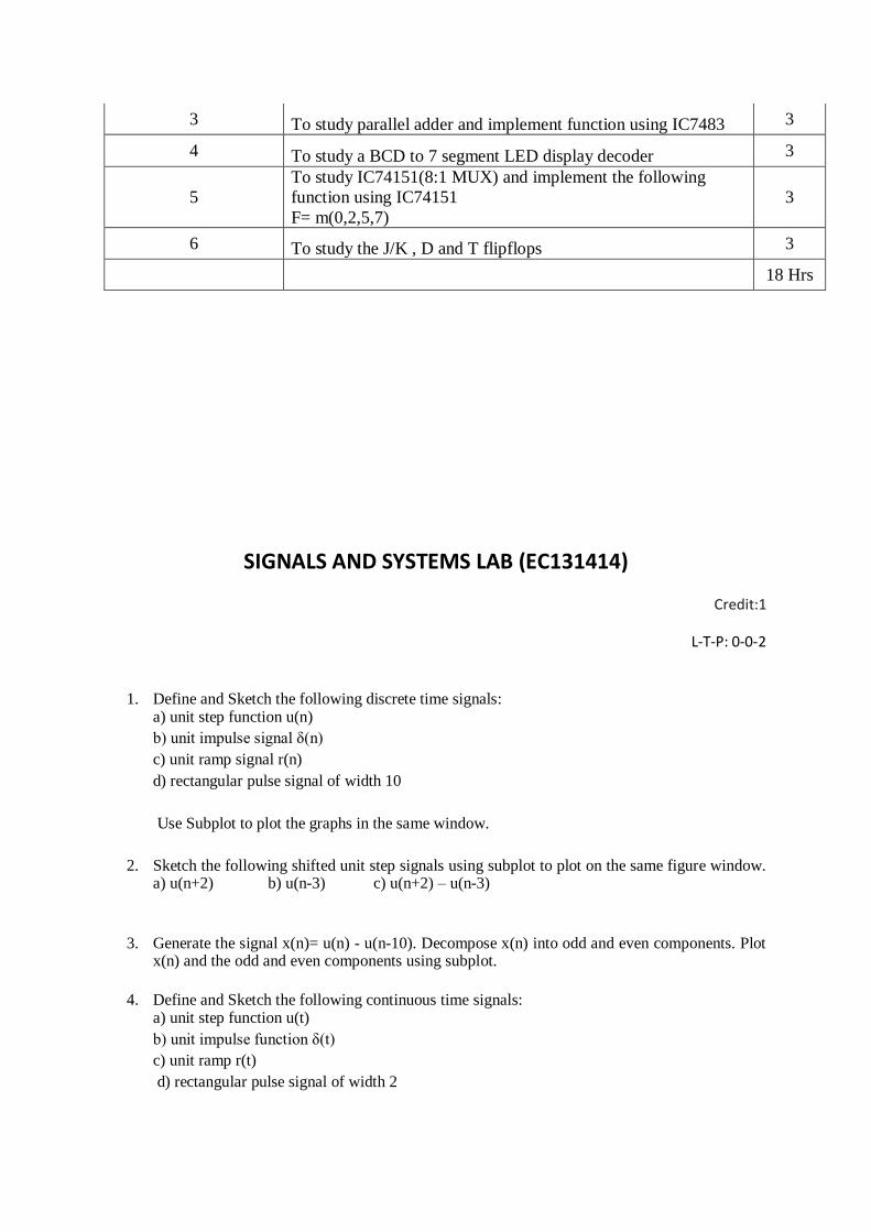
3 To study parallel adder and implement function using IC7483 3

4 To study a BCD to 7 segment LED display decoder 3

5

To study IC74151(8:1 MUX) and implement the following

function using IC74151

F= m(0,2,5,7)

3

6 To study the J/K , D and T flipflops 3

18 Hrs

SIGNALS AND SYSTEMS LAB (EC131414)

Credit:1

L-T-P: 0-0-2

1. Define and Sketch the following discrete time signals: a) unit step function u(n)

b) unit impulse signal δ(n)

c) unit ramp signal r(n)

d) rectangular pulse signal of width 10

Use Subplot to plot the graphs in the same window.

2. Sketch the following shifted unit step signals using subplot to plot on the same figure window. a) u(n+2) b) u(n-3) c) u(n+2) – u(n-3)

3. Generate the signal x(n)= u(n) - u(n-10). Decompose x(n) into odd and even components. Plot x(n) and the odd and even components using subplot.

4. Define and Sketch the following continuous time signals: a) unit step function u(t)

b) unit impulse function δ(t)

c) unit ramp r(t)

d) rectangular pulse signal of width 2

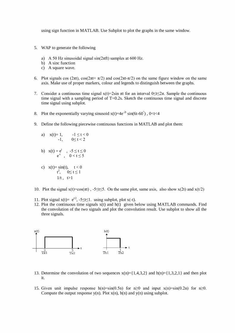
using sign function in MATLAB. Use Subplot to plot the graphs in the same window.

5. WAP to generate the following

a) A 50 Hz sinusoidal signal sin(2πft) samples at 600 Hz. b) A sinc function c) A square wave.

6. Plot signals cos (2πt), cos(2πt+ π/2) and cos(2πt-π/2) on the same figure window on the same axis. Make use of proper markers, colour and legends to distinguish between the graphs.

7. Consider a continuous time signal x(t)=2sin πt for an interval 0≤t≤2π. Sample the continuous time signal with a sampling period of T=0.2s. Sketch the continuous time signal and discrete time signal using subplot.

8. Plot the exponentially varying sinusoid x(t)=4e-2t

sin(6t-60°) , 0<t<4

9. Define the following piecewise continuous functions in MATLAB and plot them:

a) x(t)= 1, -1 ≤ t < 0 -1, 0≤ t < 2

b) x(t) = et , -5 ≤ t ≤ 0

e-t , 0 < t ≤ 5

c) x(t)= sin(t), t < 0 t

2, 0≤ t ≤ 1

1/t , t>1

10. Plot the signal x(t)=cos(πt) , -5≤t≤5. On the same plot, same axis, also show x(2t) and x(t/2)

11. Plot signal x(t)= et/2

, -5≤t≤1. using subplot, plot x(-t). 12. Plot the continuous time signals x(t) and h(t) given below using MATLAB commands. Find

the convolution of the two signals and plot the convolution result. Use subplot to show all the three signals.

13. Determine the convolution of two sequences x(n)={1,4,3,2} and h(n)={1,3,2,1} and then plot it.

15. Given unit impulse response h(n)=sin(0.5n) for n≥0 and input x(n)=sin(0.2n) for n≥0. Compute the output response y(n). Plot x(n), h(n) and y(n) using subplot.

16. Write a function to plot the unit step function and using that function plot

a) u(n), -7<n<7

b) u(n-3), -10<n<10

c) u(n+2), -6<n<6

17. WAP to find the Laplace transform of the following signals

a) t b) te-at

c) tn-1

/(n-1)! d) 3 sin(2t) + 3 cos(2t)

18. WAP to find the inverse Laplace transform of the following s-domain signals

a) 2/s(s+1)(s+2) b) 1/(s2+s+1)(s+2)

19. WAP to find the convolution of signals x(t)=t2-3t and h(t)=t using Laplace transform.

20. WAP to find the Z transform of the following signals

a) n b)an c) e

-anT d) 1+n(0.4)

n-1

21. WAP to find the inverse Z transform of the following signals

a) 1/(1-1.5z-1

+ 0.5 z-2

) b) 1/(1+z-1

)(1-z-1

)2

22. WAP to perform the convolution of the following signals x(n)=(0.4)n u(n) and h(n)=(0.5)

nu(n)

using z transform.

***************