Embed Size (px)
Citation preview

ASPRS Positional Accuracy Standards for Digital Geospatial Data
DRAFT FOR SECOND PUBLIC REVIEWDRAFT REVISION 5, VERSION 1
JULY 10, 2014
Developed by:ASPRS Map Accuracy Working Grouphttp://www.asprs.org/PAD-Division/Map-Accuracy-Standards-Working-Group.html
Comments are requested by September 15, 2014
Submit comments to: [email protected]

Rev.5 Ver.1 DRAFT – For Review Only July 10, 2014
Contents
1 Purpose1.1 Scope and applicability.................................................................................................11.2 Limitations...................................................................................................................... 11.3 Structure and format.....................................................................................................2
2 Conformance........................................................................................................................... 2
3 References............................................................................................................................... 2
4 Authority.................................................................................................................................. 3
5 Terms and definitions.............................................................................................................3
6 Symbols, abbreviated terms, and notations.........................................................................5
7 Specific requirements.............................................................................................................67.1 Check point accuracy and placement requirements..................................................77.2 Check point density and distribution...........................................................................77.3 Statistical assessment of horizontal and vertical accuracies....................................77.4 Assumptions regarding systematic errors and acceptable mean error...................77.5 Accuracy requirements for aerial triangulation and INS-based
sensor orientation of digital imagery..........................................................................87.6 Accuracy requirements for ground control used for aerial triangulation.................87.7 Horizontal accuracy requirements for digital orthoimagery......................................87.8 Horizontal accuracy requirements for digital planimetric data.................................97.9 Vertical accuracy requirements for elevation data...................................................117.10 Horizontal accuracy requirements for elevation data.............................................127.11 Low confidence areas for elevation data.................................................................137.12 Relative accuracy of lidar and IFSAR data...............................................................137.13 Reporting....................................................................................................................13
Annex A - Background (informative)......................................................................................15
Annex B - Data Accuracy and Quality Examples (normative)..............................................17B.1 Aerial Triangulation and Ground Control Accuracy Examples...............................17B.2 Digital Orthoimagery Accuracy Examples................................................................17B.3 Planimetric Data Accuracy Examples........................................................................19B.4 Relationship to the 1990 ASPRS Standards for Large Scale Maps.........................20B.5 Elevation Data Vertical Accuracy Examples.............................................................20B.6 Horizontal Accuracy Examples for Lidar Data..........................................................22B.7 Elevation Data Accuracy versus Elevation Data Quality..........................................22
Annex C - Accuracy Testing and Reporting Guidelines........................................................24C.1 Check Point Requirements.........................................................................................24C.2 Number of Check Points Required............................................................................24C.3 Distribution of Vertical Check Points across Land Cover Types............................25C.4 NSSDA Methodology for Check Point Distribution
(Horizontal and Vertical Testing) ..............................................................................26C.5 Vertical Check Point Accuracy...................................................................................26C.6 Testing and Reporting of Horizontal Accuracies......................................................26C.7 Testing and Reporting of Vertical Accuracies..........................................................26C.8 Low Confidence Areas................................................................................................27C.9 Erroneous Check Points.............................................................................................29C.10 Relative Accuracy Comparison Point Location and Criteria for Lidar Swath-to-Swath Accuracy Assessment.....................................................29
iiDRAFT – For Review Only
123456789
10111213141516171819202122232425262728293031323334353637383940414243444546474849505152535455565758

Rev.5 Ver.1 DRAFT – For Review Only July 10, 2014
Annex D - Accuracy Statistics and Example..........................................................................31D.1 NSSDA Reporting Accuracy Statistics......................................................................31D.2 Comparison with NDEP Vertical Accuracy Statistics...............................................36D.3 Computation of Percentile..........................................................................................38
FiguresFigure D.1 Error Histogram of Typical Elevation Data Set, Showing Two Outliers in Vegetated Areas...............................................................36
TablesTable 7.1 Horizontal Accuracy Standards for Digital Orthoimagery...............................9Table 7.2 Horizontal Accuracy Standards for Digital Planimetric Data.........................10Table 7.3 Vertical Accuracy Standards for Digital Elevation Data.................................11Table B.1 Aerial Triangulation and Ground Control Accuracy Requirements,
Orthophoto and/or Planimetric Data Only.................................................................17Table B.2 Aerial Triangulation and Ground Control Accuracy Requirements,
Orthophoto and/or Planimetric Data AND Elevation Data........................................17Table B.3 Horizontal Accuracy/Quality Examples for Digital Orthoimagery.................18Table B.4 Horizontal Accuracy/Quality Examples for Digital Planimetric Data............19Table B.5 Comparison of ASPRS Accuracy Standards for Planimetric Maps
at 1:1200 Scale and Digital Orthophotos with 15 cm Pixels....................................20Table B.6 Vertical Accuracy Standards for Digital Elevation Data................................20Table B.7 Lidar Density and Supported Contour Intervals for
Digital Elevation Data 22Table B.8 Expected horizontal errors (RMSEr) in Terms of Flying Altitude..................22Table C.1 Recommended Number of check Points Based on Area...............................25Table C.2 Low Confidence Areas......................................................................................29Table D.1 NSSDA Accuracy Statistics for Example Data Set with 3D Coordinates..........................................................................................................26Table D.2 Traditional Error Statistics for Example Elevation Data Set..........................43Table D.3 Comparison of NSSDA, NDEP and ASPRS Statistics
for Example Elevation Data Set...........................................................................43
iiiDRAFT – For Review Only
596061626364656667686970717273747576777879808182838485868788899091

Rev.5 Ver.1 DRAFT – For Review Only July 10, 2014
Forward
The goal of American Society for Photogrammetry and Remote sensing (ASPRS) is to advance the science of photogrammetry and remote sensing: to educate individuals in the science of photogrammetry and remote sensing; to foster the exchange of information pertaining to the science of photogrammetry and remote sensing; to develop, place into practice and maintain standards and ethics applicable to aspects of the science; to provide a means for the exchange of ideas among those interested in the sciences; to encourage, publish and distribute books, periodicals, treatises, and other scholarly and practical works to further the science of photogrammetry and remote sensing.
This standard was developed by the ASPRS Map Accuracy Standards Working Group, a joint committee under the Photogrammetric Applications Division, Primary Data Acquisition Division and Lidar Division, which was formed for the purpose of reviewing and updating ASPRS map accuracy standards to reflect current technologies. Detailed background information can be found on the Map Accuracy Working Group web page: http://www.asprs.org/PAD-Division/Map-Accuracy-Standards-Working-Group.html
ivDRAFT – For Review Only
9293949596979899
100101102103104105106

Rev.5 Ver.1 DRAFT – For Review Only July 10, 2014
ASPRS Positional Accuracy Standards for Digital Geospatial Data
1 Purpose
The objective of the ASPRS Positional Accuracy Standards for Digital Geospatial Data is to replace the existing ASPRS Accuracy Standards for Large-Scale Maps (1990), and the ASPRS Guidelines, Vertical Accuracy Reporting for Lidar Data (2004) to better address current technologies.
This standard includes positional accuracy thresholds for digital orthoimagery and digital elevation data, which are independent of published map scale or contour interval. Accuracy thresholds for planimetric data are linked to a map scale factor that which is based on the target map scale the data are designed to support. Accuracy classes have been revised and upgraded from the 1990 standard to address the higher accuracies achievable with newer technologies. The standard also includes additional accuracy measures, such as orthoimagery seam lines, aerial triangulation accuracy, lidar relative swath-to-swath accuracy, recommended minimum Nominal Pulse Density (NPD), horizontal accuracy of elevation data, delineation of low confidence areas for vertical data, and the required number and spatial distribution of QA/QC check points based on project area.
1.1 Scope and applicability
This standard addresses geo-location accuracies of geospatial products and it is not intended to cover classification accuracy of thematic maps. Further, the standard does not specify the best practices or methodologies needed to meet the accuracy thresholds stated herein. Specific requirements for the testing methodologies are specified as are some of the key elemental steps that are critical to the development of data if they are to meet these standards. However, it is the responsibility of the data provider to establish all final project design parameters, implementation steps and quality control procedures necessary to ensure the data meets final accuracy requirements.
The standard is intended to be used by geospatial data providers and users to specify the positional accuracy requirements for final geospatial products.
1.2 Limitations
This standard is limited in scope to addressing accuracy thresholds and testing methodologies for the most common mapping applications and to meet immediate shortcomings in the outdated 1990 and 2004 standards referenced above. While the standard is intended to be technology independent and broad based, there are several specific accuracy assessment needs which that were identified but are not addressed herein at this time, . These includinge:
1) Methodologies for accuracy assessment of linear features (as opposed to well defined points);
2) Rigorous total propagated uncertainty (TPU) modeling (as opposed to -- or in addition to -- ground truthing against independent data sources);
3) Robust statistics for data sets that do not meet the criteria for normally distributed data and therefore cannot be rigorously assessed using the statistical methods specified herein;
4) Image quality factors, such as edge definition and other characteristics;
5) Robust assessment of check point distribution and density;
6) Alternate methodologies to TIN interpolation for vertical accuracy assessment.
1DRAFT – For Review Only
107
108
109
110111112
113114115116117118119120121
122
123124125126127128129
130131
132
133134135136137
138
139140
141142
143
144
145

Rev.5 Ver.1 DRAFT – For Review Only July 10, 2014
This standard is intended to be the initial component upon which future work can build. Additional supplemental standards or modules should be pursued and added by subject matter experts in these fields as they are developed and approved by the ASPRS.
1.3 Structure and format
The standard is structured as follows: The primary terms and definitions, references and requirements are stated within the main body of the standard, according to the ASPRS standards template, without extensive explanation or justification. A published draft version of this standard, which includes more detailed background information and represents the critical and extensive effort and review upon which this standard was developed, was presented in narrative form in the December 2013 issue of PE&RS, pp 1073-1085, ASPRS Accuracy Standards for Digital Geospatial Data. Detailed supporting guidelines and background information are attached as Annexes A-E. Annex A provides a background summary of other standards, specifications and/or guidelines relevant to ASPRS but which do not satisfy current requirements for digital geospatial data. Annex B provides accuracy/quality examples and overall guidelines for implementing the standard. Annex C provides guidelines for accuracy testing and reporting. Annex D provides guidelines for statistical assessment and examples for computing vertical accuracy in vegetated and non-vegetated terrain.
2. Conformance
No conformance requirements are established for this standard.
3. References
American Society for Photogrammetry and Remote Sensing (ASPRS), ASPRS Accuracy Standards for Digital Geospatial Data (DRAFT), PE&RS, December 2013, pp 1073-1085
American Society for Photogrammetry and Remote Sensing (ASPRS). (1990). ASPRS Accuracy Standards for Large-Scale Maps,http://www.asprs.org/a/society/committees/standards/1990_jul_1068-1070.pdf
American Society for Photogrammetry and Remote Sensing (ASPRS), ASPRS Guidelines, Vertical Accuracy Reporting for Lidar Data, http://www.asprs.org/a/society/committees/standards/Vertical_Accuracy_Reporting_for_Lidar_Data.pdf
Dieck, R.H. (2007). Measurement uncertainty: methods and applications. Instrument Society of America, Research Triangle Park, North Carolina, 277 pp.
Federal Geographic Data Committee. (1998). FGDC-STD-007.2-1998, Geospatial Positioning Accuracy Standards, Part 2: Standards for Geodetic Networks, FGDC, c/o U.S. Geological Survey, https://www.fgdc.gov/standards/projects/FGDC-standards-projects/accuracy/part2/chapter2
Federal Geographic Data Committee. (1998). FGDC-STD-007.3-1998, Geospatial Positioning Accuracy Standards, Part 3: National Standard for Spatial Data Accuracy (NSSDA), FGDC, c/o U.S. Geological Survey, https://www.fgdc.gov/standards/projects/FGDC-standards-projects/accuracy/part3/chapter3
National Digital Elevation Program (NDEP). May 2004. NDEP Guidelines for Digital Elevation Data, http://www.ndep.gov/NDEP_Elevation_Guidelines_Ver1_10May2004.pdf
2DRAFT – For Review Only
146147148
149
150151152153154155156157158159160161
162163164165166
167168
169170171172173174175176177178179180181182183184185186187188189190

Rev.5 Ver.1 DRAFT – For Review Only July 10, 2014
National Geodetic Survey (NGS). November, 1997. NOAA Technical Memorandum NOS NGS-58, V. 4.3: Guidelines for Establishing GPS-Derived Ellipsoid Heights (Standards: 2 cm and 5 cm), https://www.ngs.noaa.gov/PUBS_LIB/NGS-58.html
Additional informative references for other relevant and related guidelines and specifications are included in Annex A.
4. Authority
The responsible organization for preparing, maintaining, and coordinating work on this guideline is the American Society for Photogrammetry and Remote Sensing (ASPRS), Map Accuracy Standards Working Group, a joint committee formed by the Photogrammetric Applications Division, Primary Data Acquisition Division and Lidar Division. For further information, contact the Division Directors using the contact information posted on the APSRS web-site, www.asprs.org.
5. Terms and definitions
absolute accuracy – A measure that accounts for all systematic and random errors in a data set.
accuracy – The closeness of an estimated value (for example, measured or computed) to a standard or accepted (true) value of a particular quantity. Not to be confused with precision.
bias – A systematic error inherent in measurements due to some deficiency in the measurement process or subsequent processing.
blunder – A mistake resulting from carelessness or negligence.
confidence level – The percentage of points within a data set that are estimated to meet the stated accuracy; e.g., accuracy reported at the 95% confidence level means that 95% of the positions in the data set will have an error with respect to true ground position that are equal to or smaller than the reported accuracy value.
consolidated vertical accuracy (CVA) – Replaced by the term Vegetated Vertical Accuracy (VVA) in this standard, CVA is the term used by the NDEP guidelines for vertical accuracy at the 95th percentile in all land cover categories combined.
fundamental vertical accuracy (FVA) – Replaced by the term Non-vegetated Vertical Accuracy (NVA), in this standard, FVA is the term used by the NDEP guidelines for vertical accuracy at the 95% confidence level in open terrain only where errors should approximate a normal error distribution.
ground sample distance (GSD) – The linear dimension of a sample pixel’s footprint on the ground. Within this document GSD is used when referring to the collection GSD of the raw image, assuming near-vertical imagery. The actual GSD of each pixel is not uniform throughout the raw image and varies significantly with terrain height and other factors. Within this document, GSD is assumed to be the value computed using the calibrated camera focal length and camera height above average horizontal terrain.
horizontal accuracy The horizontal (radial) component of the positional accuracy of a data set with respect to a horizontal datum, at a specified confidence level.
kurtosis – The measure of relative “peakedness” or flatness of a distribution compared with a normally distributed data set. Positive kurtosis indicates a relatively peaked distribution near the mean while negative kurtosis indicates a flat distribution near the mean.
local accuracy – The uncertainty in the coordinates of points with respect to coordinates of other directly connected, adjacent points at the 95% confidence level.
3DRAFT – For Review Only
191192193194195196
197
198199200201202
203
204
205206
207208
209
210211212213
214215216
217218219
220221222223224
225226
227228229
230231

Rev.5 Ver.1 DRAFT – For Review Only July 10, 2014
mean error – The average error in a set of values, obtained by adding all errors (in x, y or z) together and then dividing by the total number of errors for that dimension.
network accuracy – The uncertainty in the coordinates of mapped points with respect to the geodetic datum at the 95% confidence level.
non-vegetated vertical accuracy (NVA) – The vertical accuracy at the 95% confidence level in non-vegetated open terrain, where errors should approximate a normal distribution.
percentile – A measure used in statistics indicating the value below which a given percentage of observations (absolute values of errors) in a group of observations fall. For example, the 95th percentile is the value (or score) below which 95 percent of the observations may be found.
precision (repeatability) – The closeness with which measurements agree with each other, even though they may all contain a systematic bias.
pixel resolution or pixel size – As used within this document, pixel size is the ground size of a pixel in a digital orthoimagery product, after all rectifications and resampling procedures.
positional error – The difference between data set coordinate values and coordinate values from an independent source of higher accuracy for identical points.
positional accuracy – The accuracy at the 95% confidence level of the position of features, including horizontal and vertical positions, with respect to horizontal and vertical datums.
relative accuracy – A measure of variation in point-to-point accuracy in a data set.
resolution – The smallest unit a sensor can detect or the smallest unit an orthoimage depicts. The degree of fineness to which a measurement can be made.
root-mean-square error (RMSE) – The square root of the average of the set of squared differences between data set coordinate values and coordinate values from an independent source of higher accuracy for identical points.
skew – A measure of symmetry or asymmetry within a data set. Symmetric data will have skewness towards zero.
standard deviation – A measure of spread or dispersion of a sample of errors around the sample mean error. It is a measure of precision, rather than accuracy; the standard deviation does not account for uncorrected systematic errors.
supplemental vertical accuracy (SVA) – Merged into the Vegetated Vertical Accuracy (VVA) in this standard, SVA is the NDEP guidelines term for reporting the vertical accuracy at the 95th percentile in each separate land cover category where vertical errors may not follow a normal error distribution.
systematic error – An error whose algebraic sign and, to some extent, magnitude bears a fixed relation to some condition or set of conditions. Systematic errors follow some fixed pattern and are introduced by data collection procedures, processing or given datum.
uncertainty (of measurement) – a parameter that characterizes the dispersion of measured values, or the range in which the “true” value most likely lies. It can also be defined as an estimate of the limits of the error in a measurement (where “error” is defined as the difference between the theoretically-unknowable “true” value of a parameter and its measured value).Standard uncertainty refers to uncertainty expressed as a standard deviation.
4DRAFT – For Review Only
232233
234235
236237
238239240
241242
243244
245246
247248
249
250251
252253254
255256
257258259
260261262
263264265
266267268269270

Rev.5 Ver.1 DRAFT – For Review Only July 10, 2014
vegetated vertical accuracy (VVA) – An estimate of the vertical accuracy, based on the 95th percentile, in vegetated terrain where errors do not necessarily approximate a normal distribution.
vertical accuracy – The measure of the positional accuracy of a data set with respect to a specified vertical datum, at a specified confidence level or percentile.
For additional terms and more comprehensive definitions of the terms above, reference is made to the Glossary of Mapping Sciences.
6. Symbols, abbreviated terms, and notations
ACCr – the horizontal (radial) accuracy at the 95% confidence level
ACCz – the vertical linear accuracy at the 95% confidence level
ASPRS – American Society for Photogrammetry and Remote Sensing
CVA – Consolidated Vertical Accuracy
FVA – Fundamental Vertical Accuracy
GSD – Ground Sample Distance
GNSS - Global Navigation Satellite System
GPS – Global Positioning System
IMU – Inertial Measurement Unit
INS – Inertial Navigation System
NGPS Nominal Ground Point Spacing
NPD Nominal Pulse Density
NPS Nominal Pulse Spacing
NSSDA National Standard for Spatial Data Accuracy
NVA Non-vegetated Vertical Accuracy
QA/QC – Quality Assurance and Quality Control
RMSEr the horizontal linear RMSE in the radial direction that includes both x- and y-coordinate errors.
RMSEx the horizontal linear RMSE in the X direction (Easting)
RMSEy the horizontal linear RMSE in the Y direction (Northing)
RMSEz the vertical linear RMSE in the Z direction (Elevation)
RMSE Root Mean Square Error
RMSDz root-mean-square-difference in elevation (z)
5DRAFT – For Review Only
271272
273274
275276
277
278
279
280
281
282
283
284
285
286
287
288
289
290
291
292
293
294295
296
297
298
299
300

Rev.5 Ver.1 DRAFT – For Review Only July 10, 2014
SVA – Supplemental Vertical Accuracy
TIN – Triangulated Irregular Network
VVA Vegetated Vertical Accuracy
x sample mean error, for x
ѕ sample standard deviation
γ1 sample skewness
γ2 sample kurtosis
7. Specific requirements
This standard defines specific accuracy classes and associated RMSE thresholds for digital orthoimagery, digital planimetric data, and digital elevation data.
Testing is always recommended, but may not be required for all data sets; specific requirements must be addressed in the project specifications.
When testing is required, horizontal accuracy shall be tested by comparing the planimetric coordinates of well-defined points in the data set with coordinates of the same points from an independent source of higher accuracy. Vertical accuracy shall be tested by comparing the elevations in the data set with elevations of the same points as determined from an independent source of higher accuracy.
All accuracies are assumed to be relative to the published datum and ground control network used for the data set and as specified in the metadata. Unless specified to the contrary, it is expected that all ground control and check points should normally follow the guidelines for network accuracy as detailed in the Geospatial Positioning Accuracy Standards, Part 2: Standards for Geodetic Networks, Federal Geodetic Control Subcommittee, Federal Geographic Data Committee (FGDC-STD-007.2-1998). When local control is needed to meet specific accuracies or project needs, it must be clearly identified both in the project specifications and the metadata.
7.1 Check point accuracy and placement requirements
The independent source of higher accuracy for QA/QC check points should be at least three times more accurate than the required accuracy of the geospatial data set being tested.
A well-defined point represents a feature for which the horizontal position is known to a high degree of accuracy and position with respect to the geodetic datum. For the purpose of accuracy testing, well-defined points must be easily visible or recoverable on the ground, on the independent source of higher accuracy, and on the product itself. For testing orthoimagery, unless specifically testing for near “true-ortho” accuracies, well-defined points should not be selected on features elevated with respect to the ground surface DTM.
Elevation data sets normally do not include clearly-defined point features. Vertical accuracies are to be tested using elevations interpolated from a Triangulated Irregular Network (TIN) generated from the elevation data set. Data set elevations for testing are to be interpolated at the horizontal coordinates of the vertical check points.
6DRAFT – For Review Only
301
302
303
304
305
306
307
308309310311312313314315316317318319320321322323324325326327328329330331332333334335336337338339340341342343344345

Rev.5 Ver.1 DRAFT – For Review Only July 10, 2014
Vertical check points should be surveyed on flat or uniformly-sloped terrain, with slopes of 10% or less in order to minimize interpolation errors.
7.2 Check point density and distribution
When testing is to be performed, the distribution of the check points will be project specific and must be determined by mutual agreement between the data provider and the end user. In no case shall an NVA, digital orthophoto accuracy or planimetric data accuracy be based on less than 20 check points.
A methodology to provide quantitative characterization and specification of the spatial distribution of check points across the project extents, accounting for land cover type and project shape, is both realistic and necessary. But until such a methodology is developed and accepted, check point density and distribution will be based primarily on empirical results and simplified area based methods.
Annex C, Accuracy Testing and Reporting Guidelines, provides details on the recommended check point density and distribution. The requirements in Annex C may be superseded and updated as newer methods for determining the appropriate distribution of check points are established and approved.
7.3 Statistical assessment of horizontal and vertical accuracies
Horizontal accuracy is to be assessed using root-mean-square-error (RMSE) statistics. Vertical accuracy is to be assessed using RMSE statistics in non-vegetated terrain and 95th percentile statistics in vegetated terrain. Elevation data sets shall also be assessed for horizontal accuracy where possible, as outlined in Section 7.10.
With the exception of vertical data in vegetated terrain, error thresholds stated in this standard are presented in terms of the acceptable RMSE value. Corresponding estimates of accuracy at the 95% confidence level values are computed using National Standard for Spatial Data Accuracy NSSDA methodologies according to the assumptions and methods outlined in Annex D, Accuracy Statistics and Examples.
7.4 Assumptions regarding systematic errors and acceptable mean error
With the exception of vertical data in vegetated terrain, the assessment methods outlined in this standard, and in particular those related to computing NSSDA 95% confidence level estimates, assume that the data set errors are normally distributed and that any significant systematic errors or biases have been removed. It is the responsibility of the data provider to test and verify that the data meets those requirements. This includingrequirements includinges an evaluation of statistical parameters such as the kurtosis, skew and mean error, as well as removal of systematic errors or biases in order to achieve an acceptable mean error prior to delivery.
The exact specification of an acceptable value for mean error may vary by project and should be negotiated between the data provider and the client. These standards recommend that the mean error be less than 25% of the specified RMSE value for the project. If a larger mean error is negotiated as acceptable, this should be documented in the metadata. In any case, mean errors that are greater than 25% of the target RMSE, whether identified pre-delivery or post-delivery, should be investigated to determine the cause and what actions, if any, should be taken, and then. This should be documented in the metadata.
Where RMSE testing is performed, discrepancies between the x, y or z coordinates of the ground point, as determined from the data set and by the check survey, that exceed three times the specified RMSE
7DRAFT – For Review Only
346347348349350
351352353
354355356357358359360361362363364365366367368369370371372373374375376377378379380381382383384385386387388389390391392393394395

Rev.5 Ver.1 DRAFT – For Review Only July 10, 2014
error threshold shall be interpreted as blunders and should be investigated and either corrected or explained before the map is considered to meet this standard. Blunders may not be discarded without proper investigation and explanation.
7.5 Accuracy requirements for aerial triangulation and INS-based sensor orientation of digital imagery
The quality and accuracy of the aerial triangulation (if performed) and/or the Inertial Navigation System –based (INS-based) sensor orientation play a key role in determining the accuracy of final mapping products derived from digital imagery. For all photogrammetric data sets, the accuracy of the aerial triangulation or INS orientation (if used for direct orientation of the camera) should be higher than the accuracy of derived products, as evaluated at higher accuracy check points using stereo photogrammetric measurements. The standard recognizes two different criteria for aerial triangulation accuracy depending on the final derived products, those are:
Accuracy of aerial triangulation designed for digital planimetric data (orthophoto and/or digital planimetric map) only:
RMSEx(AT) or RMSEy(AT) = ½ * RMSEx(Map) or RMSEy(Map)
RMSEz(AT) = RMSEx(Map) or RMSEy(Map) of orthophoto
Accuracy of aerial triangulation designed for elevation data, or planimetric data (orthophoto and/or digital planimetric map) and elevation data production:
RMSEx(AT), RMSEy(AT)or RMSEz(AT) = ½ * RMSEx(Map), RMSEy(Map)or RMSEz(DEM)
Annex B, Data Accuracy and Quality Examples, provides practical examples of these requirements.
7.6 Accuracy requirements for ground control used for aerial triangulation
Ground controls points used for aerial triangulation should have higher accuracy than the expected accuracy of derived products according to the following two categories:
Accuracy of ground controls designed for digital orthophoto and/or digital planimetric data production only:
RMSEx or RMSEy = ¼ * RMSEx or RMSEy, respectively, of orthophoto or planimetric data
RMSEz = ½ * RMSEx or RMSEy of orthophoto
Accuracy of ground controls designed for elevation data, or orthophoto and elevation data production:
RMSEx, RMSEy or RMSEz= ¼ * RMSEx, RMSEy or RMSEz, respectively, of elevation data
Annex B, Data Accuracy and Quality Examples, provides practical examples of these requirements.
7.7 Horizontal accuracy requirements for digital orthoimagery
Table 7.1 specifies three primary standard horizontal accuracy classes (Class 0, Class 1, and Class 2) applicable to digital orthoimagery. These are general classifications are used to distinguish the different
8DRAFT – For Review Only
396397398399400401402403404405406407408409410411412
413
414
415416
417
418419420421422423424425426
427
428
429430431432433434
435436437438439

Rev.5 Ver.1 DRAFT – For Review Only July 10, 2014
levels of accuracy achievable for a specific pixel size. Class 0 relates to the highest accuracy attainable with current technologies and requires specialized consideration related to ground control density, ground control accuracies and overall project design. Class 1 relates to the standard level of accuracy achievable using industry standard design parameters. Class 2 applies when less stringent design parameters are implemented (for cost savings reasons) and when higher accuracies are not needed. Classes 2 and higher are typically used for visualization-grade geospatial data. Class “N” in the table applies to any additional accuracy classes that may be needed for lower accuracy projects.
Table 7.1 Horizontal Accuracy Standards for Digital Orthoimagery
Horizontal Data
Accuracy Class
RMSEx
and RMSEy
Orthophoto Mosaic Seamline Maximum
Mismatch
0 Pixel size *1.0 Pixel size * 2.0
1 Pixel size * 2.0 Pixel size * 4.0
2 Pixel size * 3.0 Pixel size * 6.0
3 Pixel size * 4.0 Pixel size * 8.0
… … …N Pixel size *(N+1) Pixel size * 2*(N+1)
It is tThe pixel size of the final digital orthoimagery is being tested, not the Ground Sample Distance (GSD) of the raw image, that is used to establish the horizontal accuracy class.
When producing digital orthoimagery, the GSD as acquired by the sensor (and as computed at mean average terrain) should not be more than 95% of the final orthoimagery pixel size. In extremely steep terrain, additional consideration may need to be given to the variation of the GSD across low lying areas in order to ensure that the variation in GSD across the entire image does not significantly exceed the target pixel size.
As long as proper low-pass filtering1 is performed prior to decimation (reduction of the sampling rate), orthophotos can be down-sampled (meaning increasing the pixel size) from the raw image GSD to any ratio that is agreed upon between the data provider and the data user, such as when imagery with 15 cm GSD is used to produce orthophotos with 30 cm pixels.
Annex B, Data Accuracy and Quality Examples, provides horizontal accuracy examples and other quality criteria for digital orthoimagery for a range of common pixel sizes.
7.8 Horizontal accuracy requirements for digital planimetric data
Table 7.2 specifies three primary ASPRS horizontal accuracy classes (Class 0, Class 1 and Class 2) applicable to planimetric maps compiled at any target map scale.
Accuracies are based on the Map Scale Factor, which is defined as the reciprocal of the ratio used to specify the metric map scale for which the data are intended to be used. Class 0 accuracies were established as 1.25% of the Map Scale Factor (or 0.0125 * Map Scale Factor). These requirements reflect accuracies achievable with current digital imaging, triangulation, and geopositioning technologies.
1 Digital sampling requires that a signal be “band-limited” prior to sampling to prevent aliasing (blending or “folding” high frequencies into the desired lower frequency). This band limiting is accomplished by employing a frequency limiting (low pass) filter.
9DRAFT – For Review Only
440441442443444445446447448
449450451452453454455456457458459460461462463464465466467468469470471472473474475
123

Rev.5 Ver.1 DRAFT – For Review Only July 10, 2014
Accuracies for subsequent accuracy classes are a direct multiple of the Class 0 values (e.g., Class 1 accuracies are two times the Class 0 value, Class 2 accuracies are three times the Class 0 value, etc.).
Table 7.2 Horizontal Accuracy Standards for Digital Planimetric Data
Horizontal Data Accuracy Class
RMSEx and RMSEy(cm)
0 0.0125 * Map Scale Factor
1 0.025 * Map Scale Factor
2 0.0375 * Map Scale Factor
3 0.05 * Map Scale Factor
... …
N (N+1)* 0.0125 *Map Scale Factor
While it is true that digital data can be plotted or viewed at any scale, map scale as used in these standards refers specifically to the target map scale that the project was designed to support. For example, if a map was compiled for use or analysis at a scale of 1:1,200 or 1/1,200, the Map Scale Factor is 1,200. RMSE in X or Y (cm) = 0.0125 times the Map Scale Factor, or 1,200 * 0.0125 = 15 cm.
The 0.0125, 0.025 and 0.0375 multipliers in Table 7.2 are not unit-less; they apply only to RMSE values computed in centimeters. Appropriate conversions must be applied to compute RMSE values in other units.
The source imagery, control and data compilation methodology will determine the level of map scale detail and accuracy that can be achieved. Factors will include sensor type, imagery GSD, control, and aerial triangulation methodologies. Multiple classes are provided for situations where a high level of detail can be resolved at a given GSD, but the sensor and/or control utilized will only support a lower level of accuracy.
As related to planimetric accuracy classes, Class 0, Class 1 and Class 2 are general classifications used to distinguish the different levels of accuracy achievable for a specific project design map scale. Class 0 relates to the highest accuracy attainable with current technologies and requires specialized consideration related to ground control density, ground control accuracies and overall project design. Class 1 relates to the standard level of accuracy achievable using industry standard design parameters. Class 2 accuracy class applies when less stringent design parameters are implemented for cost savings reasons and when higher accuracies are not needed. Classes 2 and higher are typically used for inventory level, generalized planimetry.
Although these standards are intended to primarily pertain to planimetric data compiled from stereo photogrammetry, they are equally relevant to planimetric maps produced using other image sources and technologies.
Annex B provides examples of horizontal accuracy for planimetric maps compiled at a range of common map scales.
10DRAFT – For Review Only
476477478479480
481482483484485486487488489
490491492493494
495496497498499500501502
503504505
506507

Rev.5 Ver.1 DRAFT – For Review Only July 10, 2014
7.9 Vertical accuracy requirements for elevation data
Vertical accuracy is computed using RMSE statistics in non-vegetated terrain and 95th percentile statistics in vegetated terrain. The naming convention for each vertical accuracy class is directly associated with the RMSE expected from the product. Table 7.3 provides the vertical accuracy classes naming convention for any digital elevation data. Horizontal accuracy requirements for elevation data are specified and reported independent of the vertical accuracy requirements. Section 7.10 outlines the horizontal accuracy requirements for elevation data.
Table 7.3 Vertical Accuracy Standards for Digital Elevation Data
Vertical Accuracy
Class
Absolute Accuracy Relative Accuracy (where applicable)
RMSEz
Non-Vegetated
(cm)
NVA2 at 95%
Confidence Level(cm)
VVA3 at 95th
Percentile(cm)
Within- Swath
Hard Surface Repeatability
(Max Diff)(cm)
Swath-to-Swath
Non-Vegetated Terrain(RMSDz)
(cm)
Swath-to-Swath
Non-Vegetated Terrain
(Max Diff)(cm)
X-cm ≤X ≤1.96*X ≤3.00*X ≤0.60*X ≤0.80*X ≤1.60*X
Annex B includes a discussion and listing of the applications and typical uses for each of 10 representative vertical accuracy classes. Tables B.6 and B.7 in Annex B provides vertical accuracy examples and other quality criteria for digital elevation data for those classes.
Although this standard defines the vertical accuracy independent from the contour interval measure, appropriate contour intervals are given in Table B.7 so that users can easily see the contour intervals that could be legitimately mapped from digital elevation data with the RMSEz values stated. In all cases demonstrated in Table B.7, the appropriate contour interval is three times larger than the RMSEz value, consistent with ASPRS’ 1990 standard.
The Non-vegetated Vertical Accuracy (NVA), the vertical accuracy at the 95% confidence level in non-vegetated terrain, is approximated by multiplying the RMSEz by 1.9600. This calculation includes survey check points located in traditional open terrain (bare soil, sand, rocks, and short grass) and urban terrain (asphalt and concrete surfaces). The NVA, based on an RMSEz multiplier, should be used only in non-vegetated terrain where elevation errors typically follow a normal error distribution. RMSEz-based statistics should not be used to estimate vertical accuracy in vegetated terrain or where elevation errors often do not follow a normal distribution.
2 Statistically, in non-vegetated terrain and elsewhere when elevation errors follow a normal distribution, 68.27% of errors are within one standard deviation (s) of the mean error, 95.45% of errors are within (2 * s) of the mean error, and 99.73% of errors are within (3 * s) of the mean error. The equation (1.9600 * s) is used to approximate the maximum error either side of the mean that applies to 95% of the values. Standard deviations do not account for systematic errors in the data set that remain in the mean error. Because the mean error rarely equals zero, this must be accounted for. Based on empirical results, if the mean error is small, the sample size sufficiently large and the data is normally distributed, 1.9600 * RMSEz is often used as a simplified approximation to compute the NVA at a 95% confidence level. This approximation tends to overestimate the error range as the mean error increases. A precise estimate requires a more robust statistical computation based on the standard deviation and mean error. ASPRS encourages standard deviation, mean error, skew, kurtosis and RMSE to all be computed in error analyses in order to more fully evaluate the magnitude and distribution of the estimated error.
3VVA standards do not apply to areas previously defined as low confidence areas and delineated with a low confidence polygon (see Appendix C). If VVA accuracy is required for the full data set, supplemental field survey data may be required within low confidence areas where VVA accuracies cannot be achieved by the remote sensing method being used for the primary data set.
11DRAFT – For Review Only
508
509510511512513514
515
516517518519520521522523
524525526527528529530531532533
456789
10111213
141516
17

Rev.5 Ver.1 DRAFT – For Review Only July 10, 2014
The Vegetated Vertical Accuracy (VVA), an estimate of vertical accuracy at the 95% confidence level in vegetated terrain, is computed as the 95th percentile of the absolute value of vertical errors in all vegetated land cover categories combined, . This includinges tall weeds and crops, brush lands, and fully forested areas. For all vertical accuracy classes, the VVA is 3.0 times the RMSEz.
Both the RMSEz and 95th percentile methodologies specified above are currently widely accepted in standard practice and have been proven to work well for typical elevation data sets derived from current technologies. However, both methodologies have limitations, particularly when the number of check points is small. As more robust statistical methodsthey are developed and accepted, more robust statistical methodsthey will be added as new Annexes to supplement and/or supersede these existing methodologies.
7.10 Horizontal accuracy requirements for elevation data
This standard specifies horizontal accuracy thresholds for two types of digital elevation data with different horizontal accuracy requirements:
Photogrammetric elevation data: For elevation data derived using stereo photogrammetry, the horizontal accuracy equates to the horizontal accuracy class that would apply to planimetric data or digital orthophotos produced from the same source imagery, using the same aerial triangulation/INS solution.
Lidar elevation data: Horizontal error in lidar derived elevation data is largely a function of positional error (as derived from the Global Navigation Satellite System (GNSS)), attitude (angular orientation) error (as derived from the INS) and flying altitude;, and can be estimated based on these parameters. The following equation45 provides an estimate for the horizontal accuracy for the lidar-derived data set assuming that the positional accuracy of the GNSS, the attitude accuracy of the Inertial Measurement Unit (IMU) and the flying altitude are known:
Lidar Horizontal Error (RMSE r )≈ (GNSS positional error )2+( tan( IMU error )0.55894170x flying altitude)
2
The above equation considers flying altitude (in meters), GNSS errors (radial, in cm), IMU errors (in decimal degrees), and other factors such as ranging and timing errors (which is estimated to be equal to 25% of the orientation errors). In the above equation, the values for the “GNSS positional error” and the “IMU error” can be derived from published manufacturer specifications for both the GNSS receiver and the IMU.
If the desired horizontal accuracy figure for lidar data is agreed upon, then the following equation can be used to estimate the flying altitude:
Flying Altitude ≈ 0.55894170tan ( IMU error) √(Lidar Horizontal Error (RMSEr ))2−(GNSS positional error )2
Table B.8 can be used as a guide to determine the horizontal errors to be expected from lidar data at various flying altitudes, based on estimated GNSS and IMU errors.
4The method presented here is one approach; there other methods for estimating the horizontal accuracy of lidar data sets, which are not presented herein.5Abdullah, Q., 2014, unpublished data
12DRAFT – For Review Only
534535536537538539540541542543544545546547548549550551552553554555556557558559560561562
563
564565566567568
569570571
572
573574575576
181920

Rev.5 Ver.1 DRAFT – For Review Only July 10, 2014
Guidelines for testing the horizontal accuracy of elevation data sets derived from lidar are outlined in Annex C.
Horizontal accuracies at the 95% confidence level, using NSSDA reporting methods for either “produced to meet” or “tested to meet” specifications should be reported for all elevation data sets.
For technologies or project requirements other than as specified above for photogrammetry and airborne lidar, appropriate horizontal accuracies should be negotiated between the data provider and the client. Specific error thresholds, accuracy thresholds or methods for testing will depend on the technology used and project design. It is tThe data provider has the’s responsibility to establish appropriate methodologies, applicable to the technologies used, to verify that horizontal accuracies meet the stated project requirements.
7.11 Low confidence areas for elevation data
If the VVA standard cannot be met, low confidence area polygons should be developed and explained in the metadata. For elevation data derived from imagery, the low confidence areasthis would include vegetated areas where the ground is not visible in stereo. For elevation data derived from lidar, the low confidence areasis would include dense cornfields, mangrove or similar impenetrable vegetation. The low confidence area polygonss areThis is the digital equivalent to how using dashed contours have been used in past standards and practice. Although optional, ASPRS strongly recommends the development and delivery of low confidence polygons on all lidar projects. Annex C, Accuracy Testing and Reporting Guidelines, outlines specific guidelines for implementing low confidence area polygons.
7.12 Relative accuracy of lidar and IFSAR data
For lidar and IFSAR collections, relative accuracy between swaths (inter-swath) in overlap areas is a measure of the quality of the system calibration/bore-sighting and airborne GNSS trajectories. For lidar collections, the relative accuracy within swath (intra-swath) is a measure of the repeatability of the lidar system when detecting flat, hard surfaces. The relative accuracy within swath It is also an indication of the internal stability of the instrument. Acceptable limits for relative accuracy are stated in Table 7.3.
The requirements for relative accuracy are more stringent than those for absolute accuracy.Inter-swath relative accuracy is computed as a root-mean-square-difference (RMSDz) because neither swath represents an independent source of higher accuracy (as used in RMSEz calculations). In comparing overlapping swaths, users are comparing RMS differences rather than RMS errors. Intra-swath accuracy is computed by comparing the minimum and maximum raster elevation surfaces taken over small areas of relatively flat, hard surfaces.
Annex C, Accuracy Testing and Reporting Guidelines, outlines specific criteria for selecting check point locations for inter-swath accuracies. The requirements in the annex may be superseded and updated as newer methods for determining the swath-to-swath accuracies are established and approved.
7.13 Reporting
Horizontal accuracies and NVA should be reported at the 95% confidence level according to NSSDA methodologies. VVA should be reported at the 95th percentile.
If testing is performed, accuracy statements should specify that the data are “tested to meet” the stated accuracy.
13DRAFT – For Review Only
577578579580581582583584585586587588589590591592593594595596597598599600601602603604605606607608609610611612613614615616617618
619620621622623
624625

Rev.5 Ver.1 DRAFT – For Review Only July 10, 2014
If testing is not performed, accuracy statements should specify that the data are “produced to meet” the stated accuracy. This “produced to meet” statement is. This is equivalent to the “compiled to meet” statement used by prior standards when referring to cartographic maps. The “produced to meet” method is appropriate for mature or established technologies where established procedures for project design, quality control and the evaluation of relative and absolute accuracies compared to ground control have been shown to produce repeatable and reliable results. Detailed specifications for testing and reporting to meet these requirements are outlined in Annex C.
The horizontal accuracy of digital orthoimagery, planimetric data and elevation data sets must be documented in the metadata in one of the following manners:
“Tested __ (meters, feet) horizontal accuracy at 95% confidence level.”6
“Produced to meet __ (meters, feet) horizontal accuracy at 95% confidence level.”7
The vertical accuracy of elevation data sets must be documented in the metadata in one of the following manners:
“Tested __ (meters, feet) Non-vegetated Vertical Accuracy (NVA) at 95% confidence level in all open and non-vegetated land cover categories combined using RMSEz * 1.9600.” and“Tested __ (meters, feet) Vegetated Vertical Accuracy (VVA) at the 95th percentile in all vegetated land cover categories combined using the absolute value 95th percentile error.”6
“Produced to meet __ (meters, feet) vertical accuracy at 95% confidence level.”7
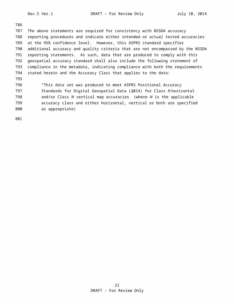
The above statements are required for consistency with NSSDA accuracy reporting procedures and indicate either intended or actual tested accuracies at the 95% confidence level. However, this ASPRS standard specifies additional accuracy and quality criteria that are not encompassed by the NSSDA reporting statements. As such, data that are produced to comply with this geospatial accuracy standard shall also include the following statement of compliance in the metadata, indicating compliance with both the requirements stated herein and the Accuracy Class that applies to the data:
“This data set was produced to meet ASPRS Positional Accuracy Standards for Digital Geospatial Data (2014) for Class N horizontal and/or Class N vertical map accuracies” (where N is the applicable accuracy class and either horizontal, vertical or both are specified as appropriate)
6 “Tested to meet” is to be used only if the data accuracies were verified by testing against independent check points of higher accuracy.
7 “Produced to meet” should be used by the data provider to assert that the data meets the specified accuracies, based on established processes that produce known results, but that independent testing against check points of higher accuracy was not performed.
14DRAFT – For Review Only
626627628629630631632
633634635636637638639640641642643644645646647648649650651652653654655656657658
659
2122
232425

Rev.5 Ver.1 DRAFT – For Review Only July 10, 2014
Annex A — Background
(informative)
Accuracy standards for geospatial data have broad applications nationally and/or internationally, whereas specifications provide technical requirements/acceptance criteria that a geospatial product must conform to in order to be considered acceptable for a specific intended use. Guidelines provide recommendations for acquiring, processing and/or analyzing geospatial data, normally intended to promote consistency and industry best practices.
The following is a summary of standards, specifications and guidelines relevant to ASPRS but which do not fully satisfy current requirements for accuracy standards for digital geospatial data:
The National Map Accuracy Standard (NMAS) of 1947 established horizontal accuracy thresholds for the Circular Map Accuracy Standard (CMAS) as a function of map scale, and vertical accuracy thresholds for the Vertical Map Accuracy Standard (VMAS) as a function of contour interval – both reported at the 90% confidence level. Because NMAS accuracy thresholds are a function of the map scale and/or contour interval of a printed map, they are inappropriate for digital geospatial data where scale and contour interval are changed with a push of a button while not changing the underlying horizontal and/or vertical accuracy.
The ASPRS 1990 Accuracy Standards for Large-Scale Maps established horizontal and vertical accuracy thresholds in terms of RMSE values in X, Y and Z at ground scale. However, because the RMSE thresholds for Class 1, Class 2 and Class 3 products pertain to printed maps with published map scales and contour intervals, these ASPRS standards from 1990 are similarly inappropriate for digital geospatial data.
The National Standard for Spatial Data Accuracy (NSSDA), published by the Federal Geographic Data Committee (FGDC) in 1998, was developed to report accuracy of digital geospatial data at the 95% confidence level as a function of RMSE values in X, Y and Z at ground scale, unconstrained by map scale or contour interval. The NSSDA states, “The reporting standard in the horizontal component is the radius of a circle of uncertainty, such that the true or theoretical location of the point falls within that circle 95% of the time. The reporting standard in the vertical component is a linear uncertainty value, such that the true or theoretical location of the point falls within +/- of that linear uncertainty value 95% of the time. The reporting accuracy standard should be defined in metric (International System of Units, SI) units. However, accuracy will be reported in English units(inches and feet) where point coordinates or elevations are reported in English units …The NSSDA uses root-mean-square error (RMSE) to estimate positional accuracy …Accuracy reported at the 95% confidence level means that 95% of the positions in the data set will have an error with respect to true ground position that is equal to or smaller than the reported accuracy value.” The NSSDA does not define threshold accuracy values, stating, “Agencies are encouraged to establish thresholds for their product specifications and applications and for contracting purposes.” In its Appendix 3-A, the NSSDA provides equations for converting RMSE values in X, Y and Z into horizontal and vertical accuracies at the 95% confidence levels. The NSSDA assumes normal error distributions with systematic errors eliminated as best as possible.
The National Digital Elevation Program (NDEP) published the NDEP Guidelines for Digital Elevation Data in 2004, recognizing that lidar errors of Digital Terrain Models (DTMs) do not necessarily follow a normal distribution in vegetated terrain. The NDEP developed Fundamental Vertical Accuracy (FVA), Supplemental Vertical Accuracy (SVA) and Consolidated Vertical Accuracy (CVA). The FVA is computed in non-vegetated, open terrain only, based on the NSSDA’s RMSEz * 1.9600 because elevation errors in open terrain do tend to follow a normal distribution, especially with a large number of check points. SVA is computed in individual land cover categories, and CVA is computed in all land cover categories combined ─ both based on
15DRAFT – For Review Only
660661
662
663664665666667
668669
670671672673674675676
677678679680681
682683684685686687688689690691692693694695696697698699
700701702703704705706707

Rev.5 Ver.1 DRAFT – For Review Only July 10, 2014
95th percentile errors (instead of RMSE multipliers) because errors in DTMs in other land cover categories, especially vegetated/forested areas, do not necessarily follow a normal distribution. The NDEP Guidelines, while establishing alternative procedures for testing and reporting the vertical accuracy of elevation data sets when errors are not normally distributed, also do not provide accuracy thresholds or quality levels.
The ASPRS Guidelines: Vertical Accuracy Reporting for Lidar Data, published in 2004, essentially endorsed the NDEP Guidelines, to include FVA, SVA and CVA reporting. Similarly, the ASPRS 2004 Guidelines, while endorsing the NDEP Guidelines when elevation errors are not normally distributed, also do not provide accuracy thresholds or quality levels.
Between 1998 and 2010, the Federal Emergency Management Agency (FEMA) published Guidelines and Specifications for Flood Hazard Mapping Partners that included RMSEz thresholds and requirements for testing and reporting the vertical accuracy separately for all major land cover categories within floodplains being mapped for the National Flood Insurance Program (NFIP). With its Procedure Memorandum No. 61 ─ Standards for Lidar and Other High Quality Digital Topography, dated September 27, 2010, FEMA endorsed the USGS Draft Lidar Base Specifications V13, relevant to floodplain mapping in areas of highest flood risk only, with poorer accuracy and point density in areas of lesser flood risks. USGS’ draft V13 specification subsequently became the final USGS Lidar Base Specification V1.0 specification summarized below. FEMA’s Guidelines and Procedures only address requirements for flood risk mapping and do not represent accuracy standards that are universally applicable.
In 2012, USGS published its Lidar Base Specification Version 1.0, which is based on RMSEz of 12.5 cm in open terrain and elevation post spacing no greater than 1 to 2 meters. FVA, SVA and CVA values are also specified. This document is not a standard but a specification for lidar data used to populate the National Elevation Dataset (NED) at 1/9th arc-second post spacing (~3 meters) for gridded Digital Elevation Models (DEMs).
In 2012, USGS also published the final report of the National Enhanced Elevation Assessment (NEEA), which considered five Quality Levels of enhanced elevation data to satisfy nationwide requirements; each Quality Level having different RMSEz and point density thresholds. With support from the National Geospatial Advisory Committee (NGAC), USGS subsequently developed its new 3D Elevation Program (3DEP) based on lidar Quality Level 2 data with 1’ equivalent contour accuracy (RMSEz<10 cm) and point density of 2 points per square meter for all states except Alaska in which IFSAR Quality Level 5 data are specified with RMSEz between 1 and 2 meters and with 5 meter post spacing. The 3DEP lidar data are expected to be high resolution data capable of supporting DEMs at 1 meter resolution. The 3DEP Quality Level 2 and Quality Level 5 products are expected to become industry standards for digital elevation data, respectively replacing the USGS’ 1:24,000-scale topographic quadrangle map series (most of the U.S.) and the 1:63,360-scale topographic quadrangle map series (Alaska), which have been standard USGS products for nearly a century.
16DRAFT – For Review Only
708709710711712
713714715716
717718719720721722723724725726727
728729730731732
733734735736737738739740741742743744745
746

Rev.5 Ver.1 DRAFT – For Review Only July 10, 2014
Annex B — Data Accuracy and Quality Examples
(normative)
B.1 Aerial Triangulation and Ground Control Accuracy Examples
Sections 7.5 and 7.6 describe the accuracy requirements for aerial triangulation, IMU, and ground control points relative to product accuracies. These requirements differ depending on whether the products include elevation data. Tables B.1 and B.2 provide an example of how these requirements are applied in practice.
Table B.1 Aerial Triangulation and Ground Control Accuracy Requirements,Orthophoto and/or Planimetric Data Only
Product Accuracy
(RMSEx, RMSEy)(cm)
A/T Accuracy Ground Control Accuracy
RMSEx and RMSEy(cm)
RMSEz(cm)
RMSEx and RMSEy(cm)
RMSEz(cm)
50 25 50 12.5 25
Table B.2 Aerial Triangulation and Ground Control Accuracy Requirements,Orthophoto and/or Planimetric Data AND Elevation Data
Product Accuracy
(RMSEx, RMSEy,
or RMSEz)(cm)
A/T Accuracy Ground Control Accuracy
RMSEx and RMSEy(cm)
RMSEz(cm)
RMSEx and RMSEy(cm)
RMSEz(cm)
50 25 25 12.5 12.5
B.2 Digital Orthoimagery Accuracy Examples
For Class 0, Class 1 and Class 2 Horizontal Accuracy Classes, Table B.3 provides horizontal accuracy examples and other quality criteria for digital orthoimagery produced from imagery having ten common pixel sizes.
17DRAFT – For Review Only
747
748
749
750
751752753754
755756
757758759760
761762
763
764765766
767

Rev.5 Ver.1 DRAFT – For Review Only July 10, 2014
Table B.3 Horizontal Accuracy/Quality Examples for Digital Orthoimagery8
Orthophoto Pixel Size
Horizontal Data
Accuracy Class
RMSEx
or RMSEy(cm)
RMSEr
(cm)
Orthophoto Mosaic Seamline
Maximum Mismatch (cm)
Horizontal Accuracy at the 95% Confidence
Level9 (cm)
1.25 cm0 1.3 1.8 2.5 3.11 2.5 3.5 5.0 6.12 3.8 5.3 7.5 9.2
2.5 cm0 2.5 3.5 5.0 6.11 5.0 7.1 10.0 12.22 7.5 10.6 15.0 18.4
5 cm0 5.0 7.1 10.0 12.21 10.0 14.1 20.0 24.5
2 15.0 21.2 30.0 36.7
7.5 cm0 7.5 10.6 15.0 18.4
1 15.0 21.2 30.0 36.7
2 22.5 31.8 45.0 55.1
15 cm0 15.0 21.2 30.0 36.7
1 30.0 42.4 60.0 73.4
2 45.0 63.6 90.0 110.1
30 cm0 30.0 42.4 60.0 73.4
1 60.0 84.9 120.0 146.9
2 90.0 127.3 180.0 220.3
60 cm0 60.0 84.9 120.0 146.8
1 120.0 169.7 240.0 293.7
2 180.0 254.6 360.0 440.6
1 meter0 100.0 141.4 200.0 244.7
1 200.0 282.8 400.0 489.5
2 300.0 424.3 600.0 734.3
2 meter0 200.0 282.8 400.0 489.5
1 400.0 565.7 800.0 979.1
2 600.0 848.5 1200.0 1468.6
5 meter0 500.0 707.1 1000.0 1224.0
1 1000.0 1414.2 2000.0 2447.7
2 1500.0 2121.3 3000.0 3671.5
RMSEr equals the horizontal radial RMSE, i.e., √RMSEx2+RMSEy
2. All RMSE values and other accuracy parameters are in the same units as the pixel size. For example, if the pixel size is in cm, then RMSEx, RMSEy, RMSEr, horizontal accuracy at the 95% confidence level, and seamline mismatch are also in centimeters.
8 For Tables B.3, B.4, B.6, and B.7, values were rounded to the nearest mm after full calculations were performed with all decimal places
9 Horizontal (radial) accuracy at the 95% confidence level = RMSEr * 1.7308, as documented in the NSSDA.18
DRAFT – For Review Only
768
769770771772
773
2627
28

Rev.5 Ver.1 DRAFT – For Review Only July 10, 2014
B.3 Planimetric Data Accuracy ExamplesFor Class 0, Class 1 and Class 2 Horizontal Accuracy Classes, Table B.4 provides horizontal accuracy examples and other quality criteria for planimetric maps intended for use at ten common map scales:
Table B.4 Horizontal Accuracy/Quality Examples for Digital Planimetric Data
Map ScaleApproximate
Source Imagery
GSD
Horizontal Data
Accuracy Class
RMSExor
RMSEy(cm)
RMSEr
(cm)
Horizontal Accuracy at the 95% Confidence
Level (cm)
1:50 0.625 cm0 0.6 0.9 1.51 1.3 1.8 3.12 1.9 2.7 4.6
1:100 1.25 cm0 1.3 1.8 3.11 2.5 3.5 6.12 3.8 5.3 9.2
1:200 2.5 cm0 2.5 3.5 6.11 5.0 7.1 12.2
2 7.5 10.6 18.4
1:400 5 cm0 5.0 7.1 12.2
1 10.0 14.1 24.5
2 15.0 21.2 36.7
1:600 7.5 cm0 7.5 10.6 18.41 15.0 21.2 36.72 22.5 31.8 55.1
1:1,200 15 cm0 15.0 21.2 36.71 30.0 42.4 73.42 45.0 63.6 110.1
1:2,400 30 cm0 30.0 42.4 73.41 60.0 84.0 146.9
2 90.0 127.3 220.3
1:4,800 60 cm0 60.0 84.9 146.9
1 120.0 169.7 293.7
2 180.0 254.6 440.6
1:12,000 1 meter0 100.0 141.4 244.81 200.0 282.8 489.52 300.0 424.3 734.3
1:25,000 2 meter0 200.0 282.8 489.51 400.0 565.7 979.12 600.0 848.5 1468.6
Source imagery GSD cannot be universally equated to image resolution or supported accuracy. This The ability to equate GSD to image resolution or supported accuracy will vary widely with different sensors. The GSD values shown in Table B.4 are typical of the GSD required to achieve the level of detail required for the stated map scales. Achievable accuracies for a given GSD will depend upon the sensor capabilities, control, adjustment, and compilation methodologies.
19DRAFT – For Review Only
774775776
777
778
779780781782783

Rev.5 Ver.1 DRAFT – For Review Only July 10, 2014
B.4 Relationship to the 1990 ASPRS Standards for Large Scale Maps
For many, a comparative reference to the previous map standards can make the new standards more understandable. A complete cross-reference would be unwieldy in this document and can readily be compiled by the user; however, Table B.5 provides an example comparison for a single map scale and orthophoto resolution.
Table B.5 Comparison of ASPRS Accuracy Standards for
Planimetric Maps at 1:1200 Scale and Digital Orthophotos with 15 cm Pixels
ASPRS 1990 ASPRS 2014
Class Name RMSEx and RMSEy(cm) Class Name RMSEx and RMSEy
(cm)0 15
1 30 1 302 45
2 60 3 604 75
3 90 5 906 105… …N (N+1) * 15
B.5 Elevation Data Vertical Accuracy Examples
Table B.6 provides vertical accuracy examples and other quality criteria for ten vertical accuracy classes, each with appropriate contour interval supported by the RMSEz values for users that may require contours to be plotted or displayed.
Table B.6 Vertical Accuracy Standards for Digital Elevation Data
Vertical Accuracy
Class
Absolute Accuracy Relative Accuracy (where applicable)
RMSEz
Non-Vegetated
(cm)
NVA2at 95%
Confidence Level(cm)
VVA3at 95th
Percentile(cm)
Within-SwathHard Surface Repeatability
(Max Diff)(cm)
Swath-to-SwathNon-
Vegetated Terrain(RMSDz)
(cm)
Swath-to-SwathNon-
Vegetated Terrain
(Max Diff)(cm)
1-cm 1.0 2.0 3 0.6 0.8 1.6
2.5-cm 2.5 4.9 7.5 1.5 2 4
5-cm 5.0 9.8 15 3 4 8
10-cm 10.0 19.6 30 6 8 16
15-cm 15.0 29.4 45 9 12 24
20-cm 20.0 39.2 60 12 16 32
33.3-cm 33.3 65.3 100 20 26.7 53.3
20DRAFT – For Review Only
784
785
786787788789
790
791
792793794795796797798
799

Rev.5 Ver.1 DRAFT – For Review Only July 10, 2014
66.7-cm 66.7 130.7 200 40 53.3 106.7
100-cm 100.0 196.0 300 60 80 160
333.3-cm 333.3 653.3 1000 200 266.7 533.3
Table B.7 provides other quality criteria for ten vertical accuracy classes, each with appropriate contour interval supported by the RMSEz values for users that may require contours to be plotted or displayed.
Table B.7 Lidar Density and Supported Contour Intervals for Digital Elevation Data
Vertical Accuracy
Class
Absolute AccuracyRecommended
Min NPD10
(Max NPS)(pts/m2 (m))
AppropriateContourInterval
RMSEz
Non-Vegetated(cm)
NVA2at 95%
Confidence Level(cm)
1-cm 1.0 2.0 ≥20 (≤0.22) 3 cm
2.5-cm 2.5 4.9 16 (0.25) 7.5 cm
5-cm 5.0 9.8 8 (0.35) 15 cm
10-cm 10.0 19.6 2 (0.71) 30 cm
15-cm 15.0 29.4 1 (1.0) 45 cm
20-cm 20.0 39.2 0.5 (1.4) 60 cm
33.3-cm 33.3 65.3 0.25 (2.0) 1 meter
66.7-cm 66.7 130.7 0.1 (3.2) 2 meter
100-cm 100.0 196.0 0.05 (4.5) 3 meter
333.3-cm 333.3 653.3 0.01 (10.0) 10 meter
These representative vertical accuracy classes for elevation data were chosen for the following reasons:
1-cm Vertical Accuracy Class, the highest vertical accuracy class, is most appropriate for local accuracy determinations and tested relative to a local coordinate system, rather than network accuracy relative to a national geodetic network.
2.5-cm Vertical Accuracy Class, the second highest vertical accuracy class, could pertain to either local accuracy or network accuracy relative to a national geodetic network.
5 cm-Vertical Accuracy Class is equivalent to 15 cm (~6 inch) contour accuracy and approximates the accuracy class most commonly used for high accuracy engineering applications of fixed wing airborne remote sensing data.
10 cm-Vertical Accuracy Class is equivalent to 1 foot contour accuracy and approximates Quality Level 2 (QL2) from the National Enhanced Elevation Assessment (NEEA) when using airborne lidar point density of 2 points per square meter, and also serves as the basis for USGS’ 3D Elevation Program (3DEP). The NEEA’s Quality Level 1 (QL1) has the same vertical
10 Nominal Pulse Density (NPD) and Nominal Pulse Spacing (NPS) are geometrically inverse methods to measure the pulse density or spacing of a lidar collection. NPD is a ratio of the number of points to the area in which they are contained, and is typically expressed as pulses per square meter (ppsm or pts/m2). NPS is a linear measure of the typical distance between points, and is most often expressed in meters. Although either expression can be used for any data set, NPD is usually used for lidar collections with NPS <1, and NPS is used for those with NPS ≥1. Both measures are based on all 1st (or last)-return lidar point data as these return types each reflect the number of pulses. Conversion between NPD and NPS is accomplished using the equationeequation
NPS=1/√NPD and NPD=1/NPS2. Although typical point densities are listed for specified vertical accuracies, users
may select higher or lower point densities to best fit project requirements and complexity of surfaces to be modeled.21
DRAFT – For Review Only
800801802803804
805806807808809810811812813814815816817818819
2930313233343536
Rev.5 Ver.1 DRAFT – For Review Only July 10, 2014
accuracy as QL2 but with point density of 8 points per square meter. QL2 lidar specifications are found in the USGS Lidar Base Specification, Version 1.1.
15-cm Vertical Accuracy Class is equivalent to 1.5 foot contour accuracy and includes data produced to the USGS Lidar Base Specification, Version 1.0.
20-cm Vertical Accuracy Class is equivalent to 2 foot contour accuracy, approximates Quality Level 3 (QL3) from the NEEA, and covers the majority of legacy lidar data previously acquired for federal, state and local clients.
33.3-cm Vertical Accuracy Class is equivalent to 1 meter contour accuracy and approximates Quality Level 4 (QL4) from the NEEA.
66.7-cm Vertical Accuracy Class is equivalent to 2 meter contour accuracy. 100-cm Vertical Accuracy Class is equivalent to 3 meter contour accuracy, approximates
Quality Level 5 (QL5) from the NEEA, and represents the approximate accuracy of airborne IFSAR.
333.3-cm Vertical Accuracy Class is equivalent to 10 meter contour accuracy and represents the approximate accuracy of elevation data sets produced from some satellite-based sensors.
B.6 Horizontal Accuracy Examples for Lidar Data
As described in section 7.10, the horizontal errors in lidar data are largely a function of GNSS positional error, INS angular error, and flying altitude. Therefore for a given project, if the radial horizontal positional error of the GNSS is assumed to be equal to 0.11314 m (based on 0.08 m in either X or Y) and the IMU error is 0.00427 degree in roll, pitch and heading the following table can be used to estimate the horizontal accuracy of lidar derived elevation data.
Table B.8 provides estimated horizontal errors, in terms of RMSEr, as computed by the equation in section 7.10 for different flying altitudes above mean terrain.
Table B.8 Expected horizontal errors (RMSEr) in terms of flying altitude
Altitude(m)
Positional RMSEr
(cm)Altitude
(m)Positional RMSEr
(cm)500 13.1 3,000 41.6
1,000 17.5 3,500 48.01,500 23.0 4,000 54.52,000 29.0 4,500 61.12,500 35.2 5,000 67.6
Different lidar systems in the market have different specifications for the GNSS and IMU and therefore, the values in Table B.8 should be modified according to the equation in section 7.10.
B.7 Elevation Data Accuracy versus Elevation Data Quality
In aerial photography and photogrammetry, the accuracy of the individual points in a data set is largely dependent on the scale and resolution of the source imagery. Larger scale imagery, flown at a lower altitude, produces smaller GSDs and higher measurement accuracies (both vertical and horizontal). Users have quite naturally come to equate higher density imagery (smaller GSD or smaller pixel sizes) with higher accuracies and higher quality.
In airborne topographic lidar, this is not entirely the case. For many typical lidar collections, the maximum accuracy attainable, theoretically, is now limited by physical error budgets of the different components of the lidar system such as laser ranging, the GNSS, the IMU, and the encoder systems. Increasing the density of points does not change those factors. Beyond the physical error budget limitations, all data must also be properly controlled, calibrated, boresighted, and processed. Errors introduced during any of
22DRAFT – For Review Only
820821822823824825826827828829830831832833834835836
837838839840841
842843
844
845
846847
848
849850851852853
854855856857858

Rev.5 Ver.1 DRAFT – For Review Only July 10, 2014
these steps will affect the accuracy of the data, regardless of how dense the data are. That said, high density lidar data are usually of higher quality than low density data, and the increased quality can manifest as apparently higher accuracy.
In order to accurately represent a complex surface, denser data are necessary to capture the surface details for accurate mapping of small linear features such as curbs and micro drainage features, for example. This The use of denser data for complex surface representation does not make the individual lidar measurements any more accurate, but does improve the accuracy of the derived surface at locations between the lidar measurements (as each reach between points is shorter).
In vegetated areas, where many lidar pulses are fully reflected before reaching the ground, a higher density data set tends to be more accurate because more points will penetrate through vegetation to the ground. More ground points will result in less interpolation between points and improved surface definition because more characteristics of the actual ground surface are being measured, not interpolated. This The use of more ground points is more critical in variable or complex surfaces, such as mountainous terrain, where generalized interpolation between points would not accurately model all of the changes in the surface.
Increased density may not improve the accuracy in flat, open terrain where interpolation between points would still adequately represent the ground surface. However, in areas where denser data may not be necessary to improve the vertical accuracy of data, a higher density data set may still improve the quality of the data by adding additional detail to the final surface model, by better detection of edges for breaklines, and by increasing the confidence of the relative accuracy in swath overlap areas through the reduction of interpolation existing within the data set. When lidar intensity is to be used in product derivation or algorithms, high collection density is always useful.
23DRAFT – For Review Only
859860861
862863864865866
867868869870871872873
874875876877878879880881

Rev.5 Ver.1 DRAFT – For Review Only July 10, 2014
Annex C — Accuracy Testing and Reporting Guidelines
(normative)
When errors are normally distributed, accuracy testing can be performed with RMSE values, standard deviations, mean errors, maximum and minimum errors, and unit-less skew and kurtosis values. When errors are not normally distributed, alternative methods must be used. If the number of test points (check points) is sufficient, testing and reporting can be performed using 95th percentile errors. A percentile rank is the percentage of errors that fall at or below a given value. Errors are visualized with histograms that show the pattern of errors relative to a normal error distribution.
The ability of RMSE, 95th percentile, or any other statistic to estimate accuracy at the 95% confidence level is largely dependent on the number and accuracy of the check points used to test the accuracy of a data set being evaluated. Whereas it is desirable to have 100 or more is a desirable number of check points, that number of check points may be impractical and unaffordable for many projects, especially small project areas.
C.1 Check Point Requirements
Both the total number of points and spatial distribution of check points play an important role in the accuracy evaluation of any geospatial data. Prior guidelines and accuracy standards typically specify the required number of check points and, in some cases, the land-cover types, but there is no requirement for defining and/or characterizing the spatial distribution of the points iwas not required. While characterizing the point distribution it is not a simple process and there is no practical method is available at this time, characterizing the point distribution by some measure and, consequently, providing a quality number is undoubtedly both realistic and necessary. ASPRS encourages research into this topic, peer reviewed and published in Photogrammetric Engineering and Remote Sensing for public testing and comment.
Until a quantitative characterization and specification of the spatial distribution of check points across a project is developed, more general methods of determining an appropriate check point distribution must be implemented. In the interim, this Annex provides general recommendations and guidelines related to the number of check points, distribution of across land cover types and spatial distribution.
C.2 Number of Check Points Required
Table C.1 lists ASPRS recommendations for the number of check points to be used for vertical and horizontal accuracy testing of elevation data sets and for horizontal accuracy testing of digital orthoimagery and planimetric data sets.
Table C.1 Recommended Number of Check Points Based on Area
Project Area (Square
Kilometers)
Horizontal Accuracy Testing of Orthoimagery
and PlanimetricsVertical and Horizontal Accuracy Testing of Elevation
Data sets
Total Number of Static 2D/3D Check Points
(clearly-defined points)
Number of Static 3D Check Points
in NVA11
Number of Static 3D Check Points in VVA
Total Number of Static 3D Check
Points≤500 20 20 5 25
501-750 25 20 10 30751-1000 30 25 15 40
1001-1250 35 30 20 501251-1500 40 35 25 601501-1750 45 40 30 70
11 Although vertical check points are normally not well defined, where feasible, the horizontal accuracy of lidar data sets should be tested by surveying approximately half of all NVA check points at the ends of paint stripes or other point features that are visible and can be measured on lidar intensity returns.
24DRAFT – For Review Only
882
883
884885886887888889
890891892893894
895
896
897898899900901902903904
905906907908
909
910911912
913
373839

Rev.5 Ver.1 DRAFT – For Review Only July 10, 2014
1751-2000 50 45 35 802001-2250 55 50 40 902251-2500 60 55 45 100
Using metric units, ASPRS recommends 100 static vertical check points for the first 2500 square kilometer area within the project. This, which provides a statistically defensible number of samples on which to base a valid vertical accuracy assessment.
For horizontal testing of areas >2500 km2, clients should determine the number of additional horizontal check points, if any, based on criteria such as resolution of imagery and extent of urbanization.
For vertical testing of areas >2500 km2, add 5 additional vertical check points for each additional 500 km2
area. Each additional set of 5 vertical check points for 500 km2 would include 3 check points for NVA and 2 for VVA. The recommended number and distribution of NVA and VVA check points may vary depending on the importance of different land cover categories and client requirements.
C.3 Distribution of Vertical Check Points across Land Cover Types
In contrast to the recommendations in Table C.1, both the 2003 and the current FEMA guidelines reference the five general land cover types, and specify a minimum of 20 check points in each of three to five land cover categories as they exist within the project area, for a total of 60-100 check points. Under the current FEMA guidelines, this quantity applies to each 2000 square mile area, or partial area, within the project.
ASPRS recognizes that some project areas are primarily non-vegetated, whereas other areas are primarily vegetated. For these reasons, the distribution of check points can vary based on the general proportion of vegetated and non-vegetated area in the project. Check points should be distributed generally proportionally among the various vegetated land cover types in the project.
C.4 NSSDA Methodology for Check Point Distribution (Horizontal and Vertical Testing)
The NSSDA offers a method that can be applied to projects that are generally rectangular in shape and are largely non-vegetated. These methods do not apply to the irregular shapes of many projects or to most vegetated land cover types. The NSSDA specifies the following:
“Due to the diversity of user requirements for digital geospatial data and maps, it is not realistic to includinge statements in this standard that specify the spatial distribution of check points is not realistic. Data and/or map producers must determine check point locations.
“Check points may be distributed more densely in the vicinity of important features and more sparsely in areas that are of little or no interest. When data exist for only a portion of the data set, confine test points to that area. When the distribution of error is likely to be nonrandom, it may be desirable to locate check points to correspond to the error distribution.
“For a data set covering a rectangular area that is believed to have uniform positional accuracy, check points may be distributed so that points are spaced at intervals of at least 10% of the diagonal distance across the data set and at least 20% of the points are located in each quadrant of the data set. (FGDC, 1998)”12
12 Federal Geographic Data Committee. (1998). FGDC-STD-007.3-1998, Geospatial Positioning Accuracy Standards, Part 3: National Standard for Spatial Data Accuracy, FGDC, c/o U.S. Geological Survey, www.fgdc.fgdc.gov/standards/documents/standards/accuracy/chapter3.pdf.
25DRAFT – For Review Only
914
915916917
918919
920921922923
924
925926927928929
930931932933
934
935936937
938939940941942943944945946947948949950951952953
404142
43

Rev.5 Ver.1 DRAFT – For Review Only July 10, 2014
ASPRS recommends that, where appropriate and to the highest degree possible, the NSSDA method be applied to the project and incorporated land cover type areas. In some areas, access restrictions may prevent the desired spatial distribution of check points across land cover types; difficult terrain and transportation limitations may make some land cover type areas practically inaccessible. Where it is not geometrically or practically applicable to strictly apply the NSSDA method, data vendors should use their best professional judgment to apply the spirit of that method in selecting locations for check points.
Clearly, the recommendations in sections C.1 through C.3 offer a good deal of discretion in the location and distribution of check points, and this is intentional. It would not be worthwhile to locate 50 vegetated check points in a fully urbanized county such as Orange County, California; 80 non-vegetated check points might be more appropriate. Likewise, projects in areas that are overwhelmingly forested with only a few small towns might support only 20 non-vegetated check points. In some areas, access restrictions may prevent the desired spatial distribution of check points; difficult terrain and transportation limitations may make some land cover type area practically inaccessible. Vendors are expected to use their best professional judgment in determining quantity and locations of check points.
The general location and distribution of check points should be discussed between and agreed upon by the vendor and customer as part of the project plan.
C.5 Vertical Check Point Accuracy
Vertical check points need not be clearly-defined point features. Kinematic check points, which are less accurate than static check points, can be used in any quantity as supplemental data, but the core accuracy assessment must be based on static surveys, consistent with NOAA Technical Memorandum NOS NGS-58, Guidelines for Establishing GPS-Derived Ellipsoid Heights (Standards: 2 cm and 5 cm), or equivalent. NGS-58 establishes ellipsoid height accuracies of 5 cm at the 95% confidence level for network accuracies relative to the geodetic network, as well as ellipsoid height accuracies of 2 cm and 5 cm at the 95% confidence level for accuracies relative to local control.
As with horizontal accuracy testing, vertical QA/QC check points should be three times more accurate than the required accuracy of the elevation data set being tested.
C.6 Testing and Reporting of Horizontal Accuracies
When errors are normally distributed and the mean is small, ASPRS endorses the NSSDA procedures for testing and reporting the horizontal accuracy of digital geospatial data. The NSSDA methodology applies to most digital orthoimagery and planimetric data sets where systematic errors and bias have been appropriately removed. Accuracy statistics and examples are outlined in more detail in Annex D.
Elevation data sets do not always contain the type of well-defined points that are required for horizontal testing to NSSDA specifications. Specific methods for testing and verifying horizontal accuracies of elevation data sets depend on technology used and project design.
For horizontal accuracy testing of lidar data sets, at least half of the NVA vertical check points should be located at the ends of paint stripes or other point features visible on the lidar intensity image, allowing them to double as horizontal check points. The ends of paint stripes on concrete or asphalt surfaces are normally visible on lidar intensity images, as are 90-degree corners of different reflectivity, e.g., a sidewalk corner adjoining a grass surface. It is tThe data provider has the’s responsibility to establish appropriate methodologies, applicable to the technologies used, to verify that horizontal accuracies meet the stated requirements.
The specific testing methodology used should be identified in the metadata.
C.7 Testing and Reporting of Vertical Accuracies
For testing and reporting the vertical accuracy of digital elevation data, ASPRS endorses the NDEP Guidelines for Digital Elevation Data, with slight modifications from FVA, SVA and CVA procedures. This
26DRAFT – For Review Only
954955956957958959
960961962963964965966967
968969
970
971972973974975976977
978979
980
981982983984
985986987
988989990991992993994
995
996
997998

Rev.5 Ver.1 DRAFT – For Review Only July 10, 2014
ASPRS standard reports the Non-vegetated Vertical Accuracy (NVA) at the 95% confidence level in all non-vegetated land cover categories combined and reports the Vegetated Vertical Accuracy (VVA) at the 95th percentile in all vegetated land cover categories combined.
If the vertical errors are normally distributed, the sample size sufficiently large, and the mean error is sufficiently small, ASPRS endorses NSSDA and NDEP methodologies for approximating vertical accuracies at the 95% confidence level. This , which applies to NVA check points in all open terrain (bare soil, sand, rocks, and short grass) as well as urban terrain (asphalt and concrete surfaces) land cover categories.
In contrast, VVA is computed by using the 95th percentile of the absolute value of all elevation errors in all vegetated land cover categories combined, to include tall weeds and crops, brush lands, and lightly-to fully-forested land cover categories. This draws a clear distinction between non-vegetated terrain where errors typically follow a normal distribution suitable for RMSE statistical analyses, and vegetated terrain where errors do not necessarily follow a normal distribution and where the 95th percentile value more fairly estimates vertical accuracy at a 95% confidence level.
C.8 Low Confidence Areas
For stereo-compiled elevation data sets, photogrammetrists should capture two-dimensional closed polygons for “low confidence areas” where the bare-earth DTM may not meet the overall data accuracy requirements. Because photogrammetrists cannot see the ground in stereo beneath dense vegetation, in deep shadows or where the imagery is otherwise obscured, reliable data cannot be collected in those areas. Traditionally, contours within these obscured areas would be published as dashed contour lines. A compiler should make the determination as to whether the data being digitized is within NVA and VVA accuracies or not; areas not delineated by an obscure area polygon are presumed to meet accuracy standards. The extent of photogrammetrically derived obscure area polygons and any assumptions regarding how NVA and VVA accuracies apply to the photogrammetric data set must be clearly documented in the metadata.
Low confidence areas also occur with lidar and IFSAR where heavy vegetation causes poor penetration of the lidar pulse or radar signal. Although costs will be slightly higher, ASPRS recommends that “low confidence areas” for lidar be required and delivered as two-dimensional (2D) polygons based on the following four criteria:
1. Nominal ground point density (NGPD);2. Cell size for the raster analysis;3. Search radius to determine average ground point densities;4. Minimum size area appropriate to aggregate ground point densities and show a generalized low
confidence area (minimum mapping unit).
This approach describes a raster-based analysis where the raster cell size is equal to the Search Radius listed for each Vertical Data Accuracy Class. Raster results are to be converted into polygons for delivery.
This section describes possible methods for the collection or delineation of low confidence areas in elevation data sets being created using two common paradigms. Other methodologies currently exist, and additional techniques will certainly emerge in the future. The data producer may use any method they deem suitable provided the detailed technique is clearly documented in the metadata.
Table C.2 lists the values for the above low confidence area criteria that apply to each vertical accuracy class.
27DRAFT – For Review Only
99910001001
10021003100410051006
100710081009101010111012
1013
1014101510161017101810191020102110221023
1024102510261027
10281029103010311032
103310341035
1036103710381039
104010411042

Rev.5 Ver.1 DRAFT – For Review Only July 10, 2014
Table C.2 Low Confidence Areas
Vertical Accuracy
Class
RecommendedProject
Min NPD (pts/m2)(Max NPS (m))
RecommendedLow Confidence
Min NGPD (pts/m2)(Max NGPS (m))
Search Radius and Cell Size
for Computing NGPD (m)
Low Confidence PolygonsMin Area
(acres(m2))
1-cm ≥20 (≤0.22) ≥5 (≤0.45) 0.67 0.5 (2000)
2.5-cm 16 (0.25) 4 (0.50) 0.75 1 (4000)
5-cm 8 (0.35) 2 (0.71) 1.06 2 (8000)
10-cm 2 (0.71) 0.5 (1.41) 2.12 5 (20,000)
15-cm 1 (1.0) 0.25 (2.0) 3.00 5 (20,000)
20-cm 0.5 (1.4) 0.125 (2.8) 4.24 5 (20,000)
33.3-cm 0.25 (2.0) 0.0625 (4.0) 6.0 10 (40,000)
66.7-cm 0.1 (3.2) 0.025 (6.3) 9.5 15 (60,000)
100-cm 0.05 (4.5) 0.0125 (8.9) 13.4 20 (80,000)
333.3-cm 0.01 (10.0) 0.0025 (20.0) 30.0 25 (100,000)
Low confidence criteria and the values in Table C.2 are based on the following assumptions:
Ground Point Density – Areas with ground point densities less than or equal to ¼ of the recommended nominal pulse density (point per square meter) or twice the nominal pulse spacing are candidates for Low Confidence Areas. For example: a specification requires an NPS of 1 meter (or an NPD of 1 ppsm) but the elevation data in some areas resulted in a nominal ground point density of 0.25 point per square meter (nominal ground point spacing of 2 meters). Such areas are good candidate for “low confidence” areas.
Raster Analysis Cell Size – Because the analysis of ground point density will most likely be raster based, the cell size at which the analysis will be performed needs to be specified. It is The recommendation ised that the cell size be equals to the search radius.
Search Radius for Computing Point Densities – Because point data are being assessed, an area must be specified in order to compute the average point density within this area. The standards recommend a search area with a radius equal to 3 * NPS (not the Low Confidence NGPS). This distance is small enough to allow good definition of low density areas while not being so small as to cause the project to look worse than it really is.
Minimum Size for Low Confidence Polygons – The areas computed with low densities should be aggregated together. Unless specifically requested by clients, structures/buildings and water should be removed from the aggregated low density polygons as these features are not true Low Confidence.
Aggregated polygons greater than or equal to the stated minimum size as provided in Table C.2 should be kept and defined as Low Confidence Polygons. In certain cases, too small an area will ‘checker board’ the Low Confidence Areas; in other cases too large an area will not adequately define Low Confidence Area polygons. These determinations should be a function of the topography, land cover, and final use of the maps.
Acres were should be? used as the unit of measurement for the Low Confidence Area polygons as many agencies (USGS, NOAA, USACE, etc.) use acres as the mapping unit for required polygon collection.
28DRAFT – For Review Only
1043
1044
104510461047104810491050105110521053105410551056105710581059106010611062
10631064106510661067
10681069

Rev.5 Ver.1 DRAFT – For Review Only July 10, 2014
Approximate square meter equivalents are provided for those whose work is exclusively in the metric system. Smoothing algorithms could be applied to the Low Confidence Polygons, if desired.
There are two distinctly different types of low confidence areas:
The first types of low confidence areas are identified by the data producer – in advance – where passable identification of the bare earth is expected to be unlikely or impossible. These are areas where no control or check points should be located and where contours, if produced, should be dashed. They are exempt from accuracy assessment. Mangroves, swamps, and inundated wetland marshes are prime candidates for such advance delineation.
The second types of low confidence areas are valid VVA areas, normally forests that should also be depicted with dashed contours, but where check points should be surveyed and accuracy assessment should be performed. Such low confidence areas are delineated subsequent to classification and would usually be identifiable by the notably reduced density of bare-earth points.
This Providing Low Confidence Area polygons allows lidar data providers to protect themselves from unusable/unfair check points in swamps and protects the customer from data providers who might try to alter their data.
If reliable elevation data in low confidence areas is critical to a project, it is common practice to supplement the remote sensing data with field surveys.
C.9 Erroneous Check Points
Occasionally, a check point may “bust” at no fault of the lidar survey. Such a point may be removed from the accuracy assessment calculation:
if it is demonstrated, with pictures and descriptions, that the check point was improperly located, such as when a vertical check point is on steep terrain or within a few meters of a significant breakline that redefines the slope of the area being interpolated surrounding the check point;
if it is demonstrated and documented that the topography has changed significantly between the time the elevation data were acquired and the time the check point was surveyed; or
if (1) the point is included in the survey and accuracy reports, but not the assessment calculation, with pictures and descriptions; (2) reasonable efforts to correct the discrepancy are documented, e.g., rechecked airborne GNSS and IMU data, rechecked point classifications in the area, rechecked the ground check points; and (3) a defensible explanation is provided for discarding the point.
An explanation that the error exceeds three times the standard deviation (>3 *s) is NOT a defensible explanation.
C.10 Relative Accuracy Comparison Point Location and Criteria for Lidar Swath-to-Swath Accuracy Assessment
To the greatest degree possible, relative accuracy testing locations should meet the following criteria:
1) include all overlap areas (sidelap, endlap, and crossflights);
2) be evenly distributed throughout the full width and length of each overlap area;
3) be located in non-vegetated areas (clear and open terrain and urban areas);
29DRAFT – For Review Only
10701071
1072
10731074107510761077
107810791080108110821083108410851086
10871088
1089
10901091
109210931094
10951096
1097109810991100110111021103
110411051106110711081109111011111112111311141115
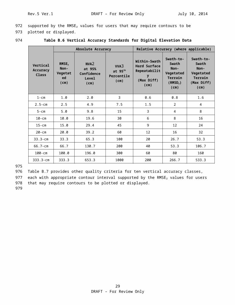
Rev.5 Ver.1 DRAFT – For Review Only July 10, 2014
4) be at least 3 meters away from any vertical artifact or abrupt change in elevation;
5) be on uniform slopes; and,
6) be within the geometrically reliable portion of both swaths (excluding the extreme edge points of the swaths). For lidar sensors with zigzag scanning patterns from oscillating mirrors, the geometrically reliable portion excludes about 5% (2½% on either side); lidar sensors with circular or elliptical scanning patterns are generally reliable throughout.
While the RMSDz value may be calculated from a set of specific test location points, the Maximum Difference requirement is not limited to these locations; it applies to all locations within the entire data set that meet the above criteria.
30DRAFT – For Review Only
1116111711181119112011211122112311241125112611271128
1129
1130
1131
1132
1133

Rev.5 Ver.1 DRAFT – For Review Only July 10, 2014
Annex D — Accuracy Statistics and Example
(normative)
D.1 NSSDA Reporting Accuracy Statistics
The National Standard for Spatial Data Accuracy (NSSDA) documents the equations for computation of RMSEx, RMSEy, RMSEr and RMSEz, as well as horizontal (radial) and vertical accuracies at the 95% confidence levels, Accuracyr and Accuracyz, respectively. These statistics assume that errors approximate a normal error distribution and that the mean error is small relative to the target accuracy.
Example on the NSSDA Accuracy Computations:For the purposes of demonstration, suppose you have five check points to verify the final horizontal and vertical accuracy for a data set (normally a minimum of 20 points would be needed). Table D.1 provides the map-derived coordinates and the surveyed coordinated for the five points. The table also shows the computed accuracy and other necessary statistics. In this abbreviated example, the data are intended to meet Class 0 planimetric accuracies for a 1:1200 target map scale (a maximum RMSEx and RMSEy of 15 cm) and the 10-cm vertical accuracy class..
Table D.1 NSSDA Accuracy Statistics for Example Data set with 3D Coordinates
31DRAFT – For Review Only
1134
1135
1136
11371138
11391140
1141114211431144114511461147
1148
1149
1150

Rev.5 Ver.1 DRAFT – For Review Only July 10, 2014
Computation of Mean Errors in x/y/z:
x= 1(n)∑i=1
n
xi
where: x iis the ith error in the specified directionn is the number of check points tested,i is an integer ranging from 1 to n.
Mean error in Easting:x = −0.140−0.100+0.017−0.070+0.1305 = -0.33 m
Mean error in Northing:y = −0.070−0.100−0.070+0.150+0.1205 = 0.006 m
Mean error in Elevation:z = −0.070+0.010+0.102−0.100+0.0875 = 0.006 m
32DRAFT – For Review Only
1151
1152
1153
1154
1155
1156
1157
1158
1159
1160
1161
1162
1163
1164
1165
11661167
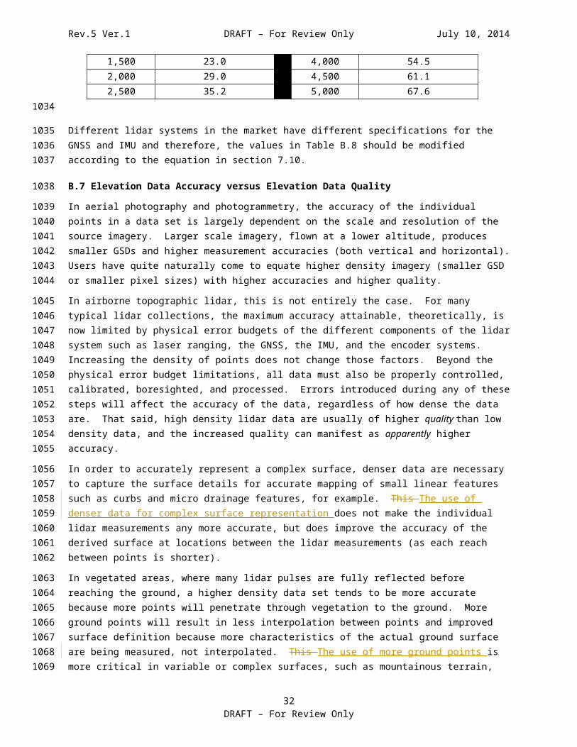
Rev.5 Ver.1 DRAFT – For Review Only July 10, 2014
Computation of Sample Standard Deviation:
sx=√ 1(n−1)∑i=1
n
(x i−x )2
where: x iis the ith error in the specified direction,x is the mean error in the specified direction,n is the number of check points tested,i is an integer ranging from 1 to n.
Sample Standard Deviation in Easting:sx=
√ (−0.140−(−0.033 ) )2+(−0.100−(−0.033 ) )2+(0.017−(−0.033 ) )2+(−0.070− (−0.033 ) )2+(0.130−(−0.033 ) )2
(5−1)
= 0.108 m
Sample Standard Deviation in Northing:sy=√ (−0.070−0.006 )2+ (−0.100−0.006 )2+ (−0.070−0.006 )2+ (0.150−0.006 )2+ (0.120−0.006 )2
(5−1)
= 0.119 m
Sample Standard Deviation in Elevation:sz=√¿¿¿
= 0.091 m
33DRAFT – For Review Only
1168
1169
1170
1171
1172
1173
1174
1175
1176
1177
1178
1179
1180
1181
1182
1183
1184
1185
1186
1187
1188
1189
1190
1191

Rev.5 Ver.1 DRAFT – For Review Only July 10, 2014
Computation of Root Mean Squares Error:
RMSE x=√ 1n∑i=1n
(x i (map)−xi (surveyed ))2
where: x i(map)is the coordinate in the specified direction of the ith check point in the data set,x i(surveyed ) is the coordinate in the specified direction of the ith check point in the independent source of higher accuracy,n is the number of check points tested,i is an integer ranging from 1 to n.
RMSE x =√¿¿¿ = 0.102 m
RMSEy=√¿¿¿ = 0.107 m
RMSE z=√¿¿¿ = 0.081 m
RMSEr=√RMSEx2+RMSEy
2
RMSEr = √¿¿ = 0.147 m
34DRAFT – For Review Only
11921193
1194
1195
1196
11971198
1199
1200
1201
1202
1203
1204
1205
1206
1207
1208
1209
1210
1211
121212131214

Rev.5 Ver.1 DRAFT – For Review Only July 10, 2014
Computation of NSSDA Accuracy at 95% Confidence Level:
(Note: There are no significant systematic biases in the measurements. The mean errors are all smaller than 25% of the specified RMSE in Northing, Easting and Elevation.)
Positional Horizontal Accuracy at 95% Confidence Level =2.4477( RMSEr
1.4142 ) = 1.7308 (RMSEr ) = 1.7308 (0.147) = 0.255 m
Vertical Accuracy at 95% Confidence Level =1.9600 (RMSE z ) = 1.9600(0.081) = 0.160 m
35DRAFT – For Review Only
1215
12161217
1218
1219
1220
1221
1222
1223
1224
1225
1226

Rev.5 Ver.1 DRAFT – For Review Only July 10, 2014
D.2 Comparison with NDEP Vertical Accuracy Statistics
Whereas the NSSDA assumes that systematic errors have been eliminated as best as possible and that all remaining errors are random errors that follow a normal distribution, the ASPRS standard recognizes that elevation errors, especially in dense vegetation, do not necessarily follow a normal error distribution, as demonstrated by the error histogram of 100 check points at Figure D.1 used as an example elevation data set for this Annex.
In vegetated land cover categories, the ASPRS standard (based on NDEP vertical accuracy statistics) uses the 95th percentile errors because a single outlier, when squared in the RMSE calculation, will unfairly distort the tested vertical accuracy statistic at the 95% confidence level. Unless errors can be found in the surveyed check point, or the location of the check point does not comply with ASPRS guidelines for location of vertical check points, such outliers should not be discarded. Instead, such outliers should be included in the calculation of the 95th percentile because: (1) the outliers help identify legitimate issues in mapping the bare-earth terrain in dense vegetation and (2) the 95 th percentile, by definition, identifies that 95% of errors in the data set have errors with respect to true ground elevation that are equal to or smaller than the 95th percentile – the goal of the NSSDA.
Example Elevation Data set
Figure D.1, plus Tables D.2 and D.3, refer to an actual elevation data set tested by prior methods compared to the current ASPRS standard.
Figure D.1 Error Histogram of Typical Elevation Data Set, Showing Two Outliers in Vegetated Areas.
Figure D.1 shows an actual error histogram resulting from 100 check points, 20 each in five land cover categories: (1) open terrain, (2) urban terrain, concrete and asphalt, (3) tall weeds and crops, (4) brush
36DRAFT – For Review Only
1227
12281229123012311232
123312341235123612371238123912401241
1242
12431244
1245
12461247124812491250

Rev.5 Ver.1 DRAFT – For Review Only July 10, 2014
lands and trees, and (5) fully forested. In this lidar example, the smaller outlier of 49 cm is in tall weeds and crops, and the larger outlier of 70 cm is in the fully forested land cover category. The remaining 98 elevation error values appear to approximate a normal error distribution with a mean error close to zero; therefore, the sample standard deviation and RMSE values are nearly identical. When mean errors are not close to zero, the sample standard deviation values will normally be smaller than the RMSE values.
Without considering the 95th percentile errors, traditional accuracy statistics, which preceded these ASPRS Positional Accuracy Standards for Digital Geospatial Data, would be as shown in Table D.2.
Note that the maximum error, skewness (γ1), kurtosis (γ2), standard deviation and RMSEz values are somewhat higher for weeds and crops because of the 49 cm outlier, and they are much higher for the fully forested land cover category because of the 70 cm outlier.
Table D.2 Traditional Error Statistics for Example Elevation Data set
Land Cover
Category
# of Check Points
Min(m)
Max(m)
Mean (m)
Mean Absolute
(m)
Median (m) γ1 γ2 ѕ
(m)RMSEz
(m)
Open Terrain 20 -0.10 0.08 -0.02 0.04 0.00 -0.19 -0.64 0.05 0.05
Urban Terrain 20 -0.15 0.11 0.01 0.06 0.02 -0.84 0.22 0.07 0.07
Weeds & Crops 20 -0.13 0.49 0.02 0.08 -0.01 2.68 9.43 0.13 0.13
Brush Lands 20 -0.10 0.17 0.04 0.06 0.04 -0.18 -0.31 0.07 0.08
Fully Forested 20 -0.13 0.70 0.03 0.10 0.00 3.08 11.46 0.18 0.17
Consoli-dated 100 -0.15 0.70 0.02 0.07 0.01 3.18 17.12 0.11 0.11
The ASPRS standards listed in Table 7.5 define two new terms: Non-vegetated Vertical Accuracy (NVA) based on RMSEz statistics and Vegetated Vertical Accuracy (VVA) based on 95th percentile statistics. The NVA consolidates the NDEP’s non-vegetated land cover categories (open terrain and urban terrain, in this example), whereas the VVA consolidates the NDEP’s vegetated land cover categories (weeds and crops, brush lands, and fully forested, in this example). Table D.3 shows ASPRS statistics and reporting methods compared to both NSSDA and NDEP.
Table D.3 Comparison of NSSDA, NDEP and ASPRS Statistics for Example Elevation Data set
Land Cover Category
NSSDA Accuracyz at 95% confidence level
based onRMSEz * 1.9600 (m)
NDEP FVA, plus SVAs and CVA
based on the 95th
Percentile (m)
NDEP Accuracy
Term
ASPRS Vertical
Accuracy (m)
ASPRS Accuracy
Term
Open Terrain 0.10 0.10 FVA0.12 NVA
Urban Terrain 0.14 0.13 SVAWeeds & Crops 0.25 0.15 SVA
0.167 VVABrush Lands 0.16 0.14 SVAFully Forested 0.33 0.21 SVAConsolidated 0.22 0.13 CVA N/A N/A
37DRAFT – For Review Only
12511252125312541255
12561257
125812591260
1261
1262126312641265126612671268
1269
1270
1271

Rev.5 Ver.1 DRAFT – For Review Only July 10, 2014
D.3 Computation of Percentile
There are different approaches to determining percentile ranks and associated values. This standard recommends the use of the following equations for computing percentile rank and percentile as the most appropriate for estimating the Vegetated Vertical Accuracy.
Note that percentile calculations are based on the absolute values of the errors, as it is the magnitude of the errors, not the sign that is of concern.
The percentile rank (n) is first calculated for the desired percentile using the following equation:
n=((( P100 )∗(N−1 ))+1)
where:n is the rank of the observation that contains the Pth percentile,P is the proportion (of 100) at which the percentile is desired (e.g., 95 for 95th percentile),N is the number of observations in the sample data set.
Once the rank of the observation is determined, the percentile (Qp) can then be interpolated from the upper and lower observations using the following equation:
Q p=( A [nw ]+(nd∗(A [nw+1 ]−A [nw ]) ))where:
Qp is the Pth percentile; the value at rank n,A is an array of the absolute values of the samples, indexed in ascending order from 1 to N,A[i] is the sample value of array A at index i (e.g., nw or nd). i must be an integer between 1 and N,n is the rank of the observation that contains the Pth percentile,nw is the whole number component of n (e.g., 3 of 3.14), nd is the decimal component of n (e.g., 0.14 of 3.14).
38DRAFT – For Review Only
1272
127312741275
12761277
1278
1279
1280
1281
12821283
1284
12851286
1287
1288
1289
12901291
12921293
1294
1295
1296
1297

Rev.5 Ver.1 DRAFT – For Review Only July 10, 2014
Example:
Given a sample data set {X1, X2 … XN} = {7, -33, -9, 5, -16, 22, 36, 37, 39, -11, 45, 28, 45, 19, -46, 10, 48, 44, 51, -27}
(N = 20),calculate the 95th percentile (P = 95):
Step 1: Take the absolute value of each observation:
{7, 33, 9, 5, 16, 22, 36, 37, 39, 11, 45, 28, 45, 19, 46, 10, 48, 44, 51, 27}Step 2: Sort the absolute values in ascending order:
A = {5, 7, 9, 10, 11, 16, 19, 22, 27, 28, 33, 36, 37, 39, 44, 45, 45, 46, 48, 51} Step 3: Compute the percentile rank n for P=95:
n=((( P100 )∗(N−1 ))+1)=((( 95100 )∗(20−1 ))+1)=19.05
The 95th percentile rank (n) of the sample data set is 19.05
Step 4: Compute the percentile value Qp by interpolating between observations 19 and 20:
Q p=(A [nw ]+(nd∗(A [nw+1 ]−A [nw ]) ))=(48+ (0.05∗(51−48 ) ) )=48.15
The 95th percentile (Qp) of the sample data set is 48.15.
39DRAFT – For Review Only
1298
1299
1300
1301
1302
1303
1304
1305
1306
1307
1308
1309
1310
1311
1312
1313
1314
1315
1316