Embed Size (px)
Citation preview

Salt intrusion at a submarine spring in a fringing reef lagoon
Sabrina M. Parra and Arnoldo Valle-Levinson, Engineering School of Sustainable Infrastructure
and Environment, University of Florida, Gainesville, Florida, USA
Ismael Mariño-Tapia, Centro de Investigación y de Estudios Avanzados del Instituto Politécnico
Nacional, Merida, Yucatan, Mexico
Cecilia Enriquez, Universidad Nacional Autónoma de México, Sisal, Yucatán, México
Corresponding author: S. M. Parra, Engineering School of Sustainable Infrastructure and
Environment, University of Florida, Weil Hall 365, Gainesville, Florida 32611, United States
Key Points:
Salt intrusion was observed during high syzygy tides
Salinities and temperatures suggest jet is connected to a stratified cave
A wave setup of 5 cm significantly reduced jet velocities and turbulence
Keywords
Salt intrusion, submarine groundwater discharge, turbulent kinetic energy, karst spring, wave
setup
Index terms: 4528 (Fronts and jets), 4568 (Turbulence), 4217 (Coastal processes), 4560 (surface
waves and tides), 4546 (nearshore processes),
Running header: Salt intrusion at a submarine spring
6 experts for review: Patricia BeddowsMatthew ReidenbachAmatzia GeninFiona WhitakerSamantha Smith
1
1
2
3
4
5
6
7
8
9
10
11
12
13
14
15
16
17
18
19
20212223242526

Acknowledgments
We thank Edgar Escalante, Francisco Ruiz and Roberto Iglesias from the Puerto Morelos
station of the Instituto de Ciencias de Mar y Limnología of Universidad Nacional Autónoma de
México for providing bathymetric and meteorological data and for the support received during
fieldwork, and Emanuel Sanchez for the support in field work. SMP gratefully acknowledges
support from the National Science Foundation’s Bridge to the Doctorate program. This research
was funded by National Science Foundation project OCE-0825876 and Consejo Nacional de
Ciencia y Tecnología, México project #84847. We would like to thank Aslak Grinsted for
allowing us the use of his MATLAB wavelet package.
2
27
28
29
30
31
32
33
34
35

Abstract (246 words)
Variations in discharge and turbulent kinetic energy (TKE) were studied at a point-source
submarine groundwater discharge (SGD), within a fringing reef lagoon, from quadrature (neap)
to syzygy (spring) tides. The principal factors affecting discharge and TKE variations were tides
and waves. Field data indicated discharge and TKE varied with high and low tides, and with
quadrature and syzygy. Maximum discharge and TKE values were observed during low tides
when the hydrostatic pressure over the jet was minimal, while the lowest discharge and TKE
values were found at high tides. Syzygy tides produced consistent saltwater intrusion during high
tides, while quadrature tides produced the greatest TKE values. In general, as the discharge
intensified during low tides, jet temperatures decreased while jet salinities increased. Decreasing
temperatures suggest that waters originated further within the aquifer. Increasing salinities of the
same discharge suggested mixing of aquifer and seawater. Therefore, it is proposed that the jet
conduit is connected to a chamber that is stratified with seawater below brackish water. The
greatest subtidal discharge occurred during quadrature tides. Syzygy produced low subtidal
discharge driven by flow reversals (flow into the aquifer) observed throughout syzygy high tides
in conjunction with the peak wave setup (>5 cm) observed during a storm. While tides were the
primary driving force of the discharge, waves played a non-negligible role. Wave effects on the
discharge were most evident during syzygy high tides combined with a storm, when the subtidal
spring discharge was weakest and salt intrusion developed.
3
36
37
38
39
40
41
42
43
44
45
46
47
48
49
50
51
52
53
54
1 Introduction
Groundwater reserves in coastal regions of the world are being threatened by sea level
rise, pollution, and ever-increasing demands for freshwater. Of special concern are coastal
aquifers because they are hydraulically connected to coastal ocean waters through the seabed.
These connections pose a fragile balance between the aquifer’s hydraulic pressure head and that
of the sea. Higher aquifer water pressure heads relative to the sea level drive submarine
groundwater discharges (SGDs) through bed sediments [Moore, 1996]. These SGDs can be
either slow diffuse sources (on the order of cm day-1) or fast point sources (on the order of m s-1)
of fresh or brackish waters [Zektser and Everett, 2000]. Diffuse (seepage) sources are associated
with low permeability bed sediments such as sandy soils {e.g.[Uchiyama et al., 2000], while
point sources (submarine springs/jets) often occur in karst topography [e.g. Valle-Levinson et al.,
[2011] and on volcanic terrain through lava tubes [e.g. Zektser and Everett, [2000];[Peterson et
al., 2009] ]. Diffuse SGDs have been studied broadly and are relevant to coastal ecosystems
because of their contribution of dissolved nutrients, both natural and anthropogenic [Taniguchi
et al., 2002; Santos et al., 2008; Moore, 2010].
Extensive study of submarine springs, on the other hand, has only occurred recently [e.g.,
[Peterson et al., 2009; Valle-Levinson et al., 2011; Expósito-Díaz et al., 2013]. In karst
topography, SGD can flow through submarine springs that provide a hydraulic connection
between seawater and aquifer water. Karst topography is found in all continents except
Antarctica. It is characterized by limestone or dolomite bedrock, where groundwater flows can
dissolve channels and caves into the predominantly calcium carbonate soil [Fleury et al., 2007].
Coastal karst aquifers also provide necessary freshwater resources to coastal communities around
the world, which are being threatened by saltwater intrusion [e.g. Fitterman, 2014]. Saltwater
4
55
56
57
58
59
60
61
62
63
64
65
66
67
68
69
70
71
72
73
74
75
76
77
intrusion is defined as “the encroachment of saline water into fresh ground water regions in
coastal aquifer settings” [Werner and Simmons, 2009].
Jet and seepage SGD in karst topography depends on the gradient between the
piezometric level and the sea level, and the contrast in densities between the aquifer water and
seawater [Valle-Levinson et al., 2011]. Some combination of these factors is necessary for salt
intrusion to occur. Conditions that affect salt intrusion from the sea include: increased sea levels
caused by storm surges [Hu et al., 2006; Smith et al., 2008], waves and wave setup [Li et al.,
1999; Parra et al., 2014], sea level rise caused by climate change [Werner and Simmons, 2009;
Vera et al., 2012; Gonneea et al., 2013], and tides [Taniguchi, 2002; Valle-Levinson et al., 2011;
Expósito-Díaz et al., 2013]. Factors from land include: seasonal variations in groundwater
recharge rates [Vera et al., 2012; Carretero et al., 2013], groundwater pumping rates from
coastal communities’ consumption [Santos et al., 2009; Ferguson and Gleeson, 2012; Carretero
et al., 2013] and the composition of sediments and porosity of coastal regions [Bakhtyar et al.,
2012]. Valle-Levinson et al., [2011] presented a few instances of salt intrusion into a point-
source SGD occurring only during the highest tides (high tide during syzygy tides). Vera et al.,
[2012] explained a more complex relationship between spring discharge and saltwater intrusion,
suggesting that lower frequency (subtidal) processes are the most influential to salt intrusion.
Additionally, groundwater flows were dominated by tides when the tidal amplitude was greatest,
while barometric pressure changes were more influential than tides during small tidal amplitudes
and relatively calm seas.
While tidal variations in submarine springs have been investigated comprehensively, the
effect of waves through wave pumping have only been quantified for seepage SGD, where wave
pumping refers to the pressure oscillations generated by pressure gradients beneath wave crests
5
78
79
80
81
82
83
84
85
86
87
88
89
90
91
92
93
94
95
96
97
98
99
100

and troughs [McLachlan and Turner, 1994]. Lab experiments showed that wind waves can
“enhance pore water and solute exchange” of diffuse SGD [Precht and Huettel, 2003]. Similar
results were obtained by numerical model results [Bakhtyar et al., 2012; Li et al., 1999]. Wave
setup has been studied in numerical models [Li et al., 1999] and with field observations [Parra
et al., 2014]. Parra et al., [2014] found that wave setup within a fringing reef lagoon acted to
suppress the discharge from a submarine spring. However, the effects of shorter frequency
waves, like wind-waves, on point-source SGD have not been studied with field observations.
Submarine groundwater discharges are known to provide nutrients and pollutant
concentrations to coastal waters and ecosystems, especially in coastal karst aquifers [Hamner
and Wolanski, 1988; Null et al., 2014; Li et al., 1999]. Ecosystems that are especially vulnerable
to and dependent on SGD-derived chemicals are coral reef ecosystems that exist in low nutrient
environments [Hamner and Wolanski, 1988]. The nutrient concentrations and subsequent
nutrient uptake by reef communities is known to depend on turbulent mixing associated with
waves and currents [Patterson et al., 1991]. However, increased pollutant transport originating
from SGD has also been shown to impact the health of coral reef and beds of seagrass worldwide
[e.g. [Metcalfe et al., 2011; Null et al., 2014; Chérubin et al., 2008]. Turbulence emanating from
submarine springs, therefore, could play an important role in nutrient and pollutant mixing, and
advection within coral reef ecosystems. Mixing can act to reduce pollutant and nutrient
concentrations to admissible levels. Understanding the levels of turbulence from point-source
SGD is needed before determining its role on the ecosystems. However, the turbulence
associated with submarine springs has been scantly studied [Parra et al., 2014; Expósito-Díaz et
al., 2013]. Expósito-Díaz et al., [2013] estimated the vertical structure of turbulent properties of
a point-source SGD in a tropical estuary in the Yucatan Peninsula. Results showed maximum
6
101
102
103
104
105
106
107
108
109
110
111
112
113
114
115
116
117
118
119
120
121
122
123

zonal Reynolds stress components, turbulent kinetic energy (TKE) production, and vertical eddy
viscosity at low tides when the greatest discharge rates were observed. Similar results showing
maximum TKE and discharge at low tides were also observed by Parra et al., [2014] at a
submarine spring located within a fringing coral reef lagoon of the Yucatan Peninsula. However,
the two previous studies have only collected 4 and 3 days of data, thus only considering tidal
variations of the discharge. Variations in turbulence at a point-source SGD from quadrature to
syzygy tides have yet to be determined.
In addition to tides and turbulence, previous studies have observed variations in seepage
SGD from syzygy through quadrature tides [Kim and Hwang, 2002; Taniguchi, 2002; Vera et
al., 2012]. Semi-monthly fluctuations in seepage SGD were more significant than originally
thought, with greater variations during syzygy or spring tides [Kim and Hwang, 2002].
Additionally, diurnal oscillations in seepage were more significant during syzygy tides than
quadrature or neap tides. Similarly, Taniguchi, [2002] found that seepage SGD varied semi-
monthly, with maximum discharge rates during syzygy tides and minimum rates during
quadrature tides.
The aim of this study is to describe fortnightly variations at a point source SGD, and to
understand the conditions of tides and waves that favor salt intrusion into the aquifer. This study
extends previous investigations by describing fortnightly variations of TKE and by determining
the additional influence of waves and wave setup on the spring discharge.
2 Methods
2.1 Study site
This study was carried out in the Puerto Morelos coral reef lagoon, located 30 km south
of Cancun on the northeast coast of the Yucatan Peninsula (Figure 1). The Yucatan Peninsula’s
7
124
125
126
127
128
129
130
131
132
133
134
135
136
137
138
139
140
141
142
143
144
145
146

watershed topography is karstic and composed of highly permeable limestone. Because of its
high permeability, rainfall quickly seeps into the aquifer. This explains the absence of surface
rivers in the region [Merino et al., 1990]. Because of the high permeability in the aquifer, the
water table has hydraulic gradients ranging from 7 to 100 mm km-1 and is known to be controlled
by sea level variations and recharge from precipitation [González-Herrera et al., 2002; Beddows
et al., 2007]. The peninsula is peppered with an abundant number of sinkholes (locally known as
cenotes), which make the unconfined aquifer visible from the surface [Vera et al., 2012]. Aquifer
waters flow within a massive network of underground caves and conduits carved through the
limestone. Eventually, aquifer waters flow into the ocean through submarine spring and seepage
discharges all along the Yucatan coast, driven by a hydraulic pressure gradient between the
aquifer and the sea. The Yucatan coastal SGDs are dominated by spring discharges, estimated at
between 78-99 % of total SGD. The Puerto Morelos lagoon has an estimated spring SGD
contribution of 78.5 %, with the remaining 21.5 % coming from seepage at the beach face [Null
et al., 2014]. Therefore, submarine springs are of great importance to the region.
Two distinct weather periods are identified in the Yucatan Peninsula region: dry and wet
(Figure 2). The dry period extends from March through June and the wet period is generally
from July through October. Between December and February, brief (2-5 days) cold fronts
characterized by northerly winds with light rains, locally known as nortes, are common. The
average rainfall is approximately 1,300 mm year-1. The time series of this study was collected
during the wet period, indicating that large aquifer recharge rates (estimated at ~25,300 hm3 year-
1) occurred throughout the watershed during this time period [Vera et al., 2012].
The Puerto Morelos lagoon has a mean water depth of ~3.5 m with a maximum depth of
8 m. It is enclosed by fringing coral reefs that are disrupted by two major and one minor inlet.
8
147
148
149
150
151
152
153
154
155
156
157
158
159
160
161
162
163
164
165
166
167
168
169
The northern inlet, locally known as Boca Grande, is 1200 m wide with a depth of 6 m, while
the central inlet, locally known as Boca Chica, is 300 m wide with a depth of 6 m. The
southern inlet is a navigation channel 400 m wide with a dredged depth of 8 m [Coronado et al.,
2007]. This lagoon is influenced by dominant semidiurnal microtides (≤0.3 m tidal range) and
persistent trade winds that drive onshore wind-waves. The reef region includes shallow
submerged coral banks which can be uncovered during low tides although it is a microtidal
region. Under normal wave conditions it is influenced by incident significant wave heights of 0.8
± 0.4 m [Coronado et al., 2007].
Puerto Morelos lagoon circulation is predominantly influenced by wind forcing and
thermohaline circulations caused by SGD and solar heat fluxes during periods of minimal wave
activity [Enriquez et al., 2012], and wind-waves (wave setup) during periods of energetic wave
conditions [Coronado et al., 2007]. Wave-driven circulation produces outflowing currents >0.5
m s-1 through the inlets, which ensures flushing and a well-mixed water column in the shallow
lagoon [Coronado et al., 2007].
The lagoon is punctuated on its bottom by numerous (10 to 15) buoyant jet discharges,
some of which can feature distinguishable surface expressions during low tides. The submarine
spring discharge of interest in this study is the Pargos spring, named after the large number of
snappers that used to congregate at this location. The spring has estimated discharge rates of
approximately 0.4 m3 s-1. It is located 300 m from shore and 1,200 m west of the central inlet
(Figure 1). The bathymetry at the spring displays an opening to the spring vent that is ~2.5 m in
diameter and extends 2 m below the lagoon floor (Figure 3). The spring vent is ~1.2 m diameter
conduit located at the bottom of the opening at an approximate depth of 7 m.
9
170
171
172
173
174
175
176
177
178
179
180
181
182
183
184
185
186
187
188
189
190
191

2.2 Data collection
In order to study the effects of the variability of tides from quadrature to syzygy and the
influence of wind-waves on the submarine spring discharge, data were collected between 19-30
July 2011, with four instruments fixed on the bed of the lagoon. Instruments were moored at
three locations: the forereef, the middle of the lagoon and at the mouth of the jet associated with
Pargos spring (Figure 1). Hydrographic recorders were moored at the spring and in mid-lagoon,
and single-point acoustic velocimeters were deployed at the spring and the forereef.
A 6 MHz Nortek Vector ADV was moored at the forereef at 2 m depth. The ADV
recorded three-dimensional velocity bottom measurements and pressure in hourly bursts of 2048
measurements at 2 Hz (~17.1 min). The water pressure measurements were used to determine
significant wave heights and corresponding spectral energy at the forereef (Figure 4).
A 6 MHz Nortek Vector acoustic Doppler velocimeter (ADV) and a Schlumberger
conductivity, temperature and depth Diver recorder (CTD) were moored at the mouth of Pargos
spring (Figure 1, 3) and gathered data simultaneously. The ADV was moored in the center of the
vent and oriented downward, while the CT was located ~25 cm above the sampling volume of
the ADV (to avoid disturbing the flow field). The ADV recorded three-dimensional velocity
point measurements and pressure in hourly bursts of 8192 measurements at 8 Hz (~17.1 min).
The water pressure bursts were used to calculate the spectral energy of the signal at the spring
(Figure 5). The three-dimensional velocity measurements were used to estimate TKE at the jet
via velocity anomalies from burst averages (Figure 6). The CTD logged point measurements of
conductivity, temperature and depth from the jet, every 10 minutes (Figure 6). Salinity was
estimated using the CTD data following the thermodynamics equation of seawater (TEOS-10)
[Millero et al., 2008].
10
192
193
194
195
196
197
198
199
200
201
202
203
204
205
206
207
208
209
210
211
212
213
214

In addition, a Sea-Bird SBE-37 conductivity and temperature recorder (CT) was deployed
on the bottom, in the middle of the lagoon (Figure 1). The CT logged measurements of
conductivity, temperature and depth every 10 minutes (Figure 6). Salinity was estimated using
the CT data following the thermodynamic equation of seawater (TEOS-10) [Millero et al., 2008].
Furthermore, hourly wind speeds and direction (Figure 4) were obtained from a meteorological
station located on shore at the Universidad Nacional Autónoma de México (UNAM) Academic
Unit.
2.3 Data processing
Incident waves at the forereef were derived from water pressure measurements (2 Hz)
obtained with an ADV using spectral analysis techniques. Spectral analysis was performed on
the water pressure data for each burst using a fast Fourier transform (FFT). In order to reduce
noise, Hanning windowing was applied to each burst. The water pressure spectra were used to
estimate significant wave heights as:
H s=4 √m0 (1)
where m0 is the zeroth moment of the spectrum based on the energy between 0.05 and 0.5 Hz. In
addition, the peak wave period, T p, was calculated based on the spectral peaks.
In this study turbulence observations were used to quantify the effects of tides and waves
on the energy of the spring discharge. Turbulent kinetic energy, k , was estimated using the
normal components of the Reynolds stress tensor as follows [Pope, 2000; Monismith, 2010]:
k=⟨ui
' 2 ⟩2
=⟨u' 2 ⟩+⟨ v' 2 ⟩+⟨ w '2 ⟩
2(2)
where the prime ( ' ) denotes velocity anomalies from the temporal mean. For example, for the x-
component the anomalies are given by u'=u−⟨U ⟩, where the brackets denote the burst mean.
11
215
216
217
218
219
220
221
222
223
224
225
226
227
228
229
230
231
232
233
234
235
236

The velocities u, v and w represent the instantaneous time series of the east, north and vertical
velocity components, respectively. TKE was calculated to seek relationships between water
surface variations, η, over the spring and spring discharge variations. Wave-turbulence
decomposition in post-processing was not performed as recommended by [Bricker and
Monismith, 2007]. They found that wave bias in turbulent velocity data was related to
uncertainties in instrument orientation (pitch, roll and compass). They recommended performing
wave-turbulence decomposition on data from instruments that do not possess compass, and
pitch/roll sensors. Therefore, data obtained from a velocimeter equipped with reliable compass
and tilt/roll sensors, like the Nortek Vector, do not require wave-turbulence decomposition
because the data produced more reliable power spectra than any method of interpolation or
filtering of the wave frequencies.
Further relationships between water surface variations and spring discharge were further
explored using wavelet analysis techniques. The continuous wavelet transform was used for
signal processing of both stationary and non-stationary datasets [Kang and Lin, 2007]. It is
similar to spectral analysis, in that it describes the contributions of oscillations at different
frequencies. While spectral analysis only considers the total contributions of an assumed-to-be-
stationary dataset, wavelet analysis is “able to determine both the dominant modes of variability
and how those modes vary in time” [Torrence and Compo, 1998]. In order to do this, wavelet
analysis decomposes a non-stationary time series into both time and frequency space. This
decomposition allows the study of both global and local processes, and therefore permits the
analysis of intermittent and aperiodic processes [Baas, 2006]. The continuous wavelet transform
was used to identify statistically significant variations in oscillations at different frequencies of
significant wave height, sea level, jet discharge and TKE throughout the time series. In this
12
237
238
239
240
241
242
243
244
245
246
247
248
249
250
251
252
253
254
255
256
257
258
259

study, a Morlet wavelet (with dimensionless frequency of 6) was used to examine the behavior in
the time-frequency domain of the variables [Torrence and Compo, 1998; Grinsted et al., 2004].
Squared coherences between water level variations and spring velocities were obtained
for a range of 0.01 to 1 Hz. The squared-coherence, γ122 ( f k ), determines the relationship between
two data sets using the cross spectral,G12 ( f k ), and auto-spectral densities,G11 ( f k ) and G22 ( f k ), as
follows [Emery and Thomson, 2001]:
γ122 ( f k )=
|G12 ( f k )|2
G11 ( f k ) G22 ( f k ) (3)
where f k are the frequencies of the squared-coherence. Considering the innate random noise
found and in order to reliably estimate the squared-coherence between two datasets, only the
coherence amplitudes that were above a 99 % confidence level were considered significant. To
reduce noise of the squared-coherence, a Hanning window was applied to the spectral densities.
3 Results
3.1 Winds and waves
During the measurement period, winds exhibited weak, moderate and storm conditions.
Weak winds were predominantly westward at ≤5 m s-1 between 19-23 July 2011 (Figure 4a).
Moderate winds were southwestward on 23-27 and 29-30 July 2011 with increased speeds of ~7
m s-1. Finally, north-northwestward winds with speeds up to 10 m s-1 occurred during a passing
storm on 28 July.
The lagoon’s circulation is known to be dominated by wind-waves (Coronado et al.
2007). The smallest significant wave heights observed at the forereef (~0.4 m) were recorded
during weak winds (Figure 4b). Increased significant wave heights (0.4-0.7 m) were observed as
winds strengthened during moderate conditions. Lastly, significant wave heights reached their
13
260
261
262
263
264
265
266
267
268
269
270
271
272
273
274
275
276
277
278
279
280
281

peak of up to 1 m on 28 July 2011 during the storm. On the other hand, peak wave periods
ranged mainly between 6 and 8 s (seconds) throughout the time series (Figure 4b).
In addition to looking at the wave heights and periods, wave energy at different
frequencies was also determined with a spectral analysis. Wave energy presented minimum
energy during the first four days and maximum energy on 28 July (Figure 4c). During weak
waves, energy was concentrated at frequencies between 0.1 and 0.3 Hz, with minimal activity at
other frequencies. As wave heights increased between 23-26 July, wave energy also increased
with a broader frequency range (0.09-0.35 Hz). Intermittent energy was also detected at lower
frequencies (<0.08 Hz), related to infragravity waves present in the lagoon and forereef (Fig 4c,
5b). Between 28-30 July as the storm passed, wave energy was at its maximum with the greatest
frequency range (0.08-0.4 Hz). Concurrently, the largest infragravity wave energy was observed.
Waves observed at the forereef (Figure 4c) had a very similar spectral signature to those at the jet
(Figure 5b) but were ~4 times greater in magnitude. The spectra of the water surface bursts at the
jet displayed waves between 0.1 and 0.3 Hz, corresponding to wind waves. However, no distinct
period of oscillation greater than the infragravity waves was observed for significant wave
heights at Pargos throughout the time series (Figure 7a).
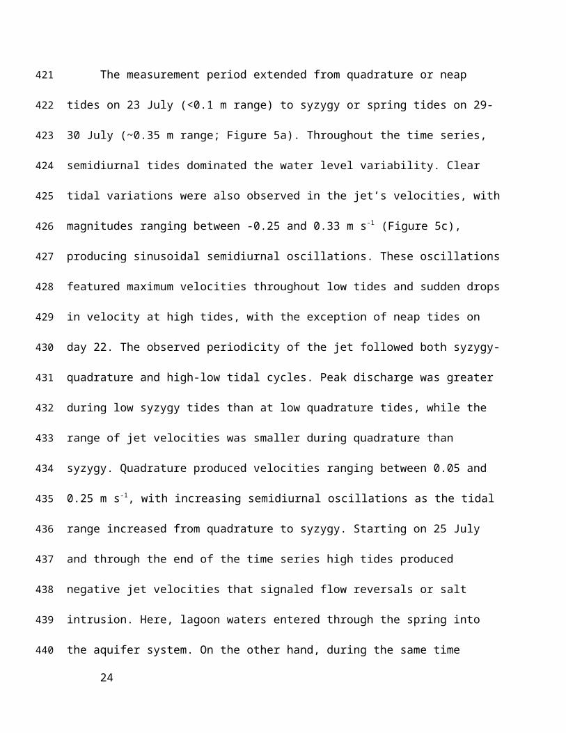
The measurement period extended from quadrature or neap tides on 23 July (<0.1 m
range) to syzygy or spring tides on 29-30 July (~0.35 m range; Figure 5a). Throughout the time
series, semidiurnal tides dominated the water level variability. Clear tidal variations were also
observed in the jet’s velocities, with magnitudes ranging between -0.25 and 0.33 m s-1 (Figure
5c), producing sinusoidal semidiurnal oscillations. These oscillations featured maximum
velocities throughout low tides and sudden drops in velocity at high tides, with the exception of
neap tides on day 22. The observed periodicity of the jet followed both syzygy-quadrature and
14
282
283
284
285
286
287
288
289
290
291
292
293
294
295
296
297
298
299
300
301
302
303
304
high-low tidal cycles. Peak discharge was greater during low syzygy tides than at low quadrature
tides, while the range of jet velocities was smaller during quadrature than syzygy. Quadrature
produced velocities ranging between 0.05 and 0.25 m s-1, with increasing semidiurnal oscillations
as the tidal range increased from quadrature to syzygy. Starting on 25 July and through the end
of the time series high tides produced negative jet velocities that signaled flow reversals or salt
intrusion. Here, lagoon waters entered through the spring into the aquifer system. On the other
hand, during the same time period low tides produced jet velocities >0.3 m s-1. The semidiurnal
oscillations of the jet discharge also appeared in the burst spectral analysis, with relatively high
values throughout the range of spectral frequencies at low tides when the discharge was the
greatest (Figure5d). Conversely, when discharge was low at high tides, the spectral signal
decreased at higher frequencies (>0.1 Hz). The squared-coherence analysis between the water
surface and spring velocities (Figure 5e) showed statistically significant coherence (within the 99
% confidence limit depicted as the black contour line) during periods of negative vertical
(downward) velocities (high tides on 26-29 July). Statistically significant coherences between
water surface and spring velocities on 26-29 July developed at the wind-wave and infragravity
wave frequencies, especially during the storm event of 28 July, revealing that wave oscillations
were observed within the jet discharge. This is known as wave pumping.
To observe the effects of waves on the lagoon circulation and spring discharge, the wave
setup was calculated as the difference between the demeaned water levels at Pargos spring and
the forereef (Figure 6b). Because the circulation in the lagoon is known to be dominated by
waves, it was expected that wave setup depended on significant wave heights. This indeed was
the case, especially during high wave events and could be explained with the following
relationship:
15
305
306
307
308
309
310
311
312
313
314
315
316
317
318
319
320
321
322
323
324
325
326
327

Δ η=0.25 H s , jet (4)
where Δ η is the wave setup between Pargos and the forereef and H s is the significant wave
height measured at the jet (r2=0.51). A greater agreement was observed after 22 July (r2=0.80),
suggesting that setup was correlated with waves only when significant wave heights became >0.4
m. However, when waves at the forereef were < 0.4 m, setup was small and dominated by other
factors.
3.2 Jet turbulent kinetic energy (TKE) and velocities
Semidiurnal variations were also evident in the jet’s turbulent kinetic energy with an
inverse relationship to tides (Figure 6c). Semidiurnal oscillations in TKE occurred throughout
most of the time series. Quadrature tides (22-24 July) allowed development of the highest values
of TKE per unit mass (up to 0.04 m2 s-2), when jet velocities remained ~0.2 m s-1 and significant
wave heights at the forereef were at their lowest (~0.4 m). Subsequent TKE maxima steadily
decreased after their peak on 23 July and as syzygy tides increased their influence on the
discharge by damping TKE development.
3.3 Jet temperature and salinity
While jet velocities and TKE oscillated inversely to the semidiurnal tides, lagoon bottom
temperatures (away from the spring’s influence) showed a diurnal pattern consistent with
atmospheric heat fluxes (Figure 6d). Between 27-29 July 2011, however, lagoon bottom
temperatures did not show diurnal oscillations, but a cooling trend most likely caused by cloud
cover from the storm. On the other hand, lagoon bottom salinities (away from the spring’s
influence) were relatively constant, starting out near 36 g kg-1 and steadily decreasing to 35.3 g
kg-1 toward the end of the time series. This could be attributed to any or a combination of the
16
328
329
330
331
332
333
334
335
336
337
338
339
340
341
342
343
344
345
346
347
348
349

following: stronger water exchange between the lagoon and the sea, decreased evaporation from
increased cloud cover, lower air temperatures, and precipitation caused by the storm (Figure 6e).
During this time of year, aquifer water temperatures are lower than ambient lagoon
temperatures, therefore jet temperatures acted as a tracer of aquifer water discharging into the
lagoon. In contrast to the ambient lagoon temperature variations, jet discharge temperatures were
clearly semidiurnal ranging from 27 to 32 °C (Figure 6d). Semidiurnal oscillations in jet
temperatures differed from quadrature to syzygy tides, with a clear transition in variability
occurring on 24 July. Throughout, high tides coincided with decreased jet flows and relatively
high water temperatures at the jet. Conversely, low tides produced increased jet discharge and
low water temperatures.
Similarly to jet temperatures, jet salinities showed semidiurnal oscillations with low
values during periods of high jet velocities (low tides). Spring salinities were generally lower
than ambient lagoon bottom salinities and also served as a conservative tracer of aquifer waters.
At Pargos spring, salinities ranged between 28 and 36 g kg-1 with clear differences between high
and low tides, and between quadrature and syzygy tides. Spring discharges were brackish,
indicating a subterranean estuary where mixing of recirculated seawater was driven by ‘tidal
pumping’ [Moore, 1999]. Tidal pumping, as defined by Santos et al., [2009], is separated into 3
components: (1) hydraulic gradient between the aquifer and the sea driving outflow during low
tides, (2) seawater recirculation or saltwater intrusion at high tide, and (3) current-driven
recirculation outside the spring. The first two components can be grouped as discharge driven by
oscillations in the water level, with the smallest sea level range at quadrature and greatest range
at syzygy tides.
17
350
351
352
353
354
355
356
357
358
359
360
361
362
363
364
365
366
367
368
369
370
371

4 Discussion
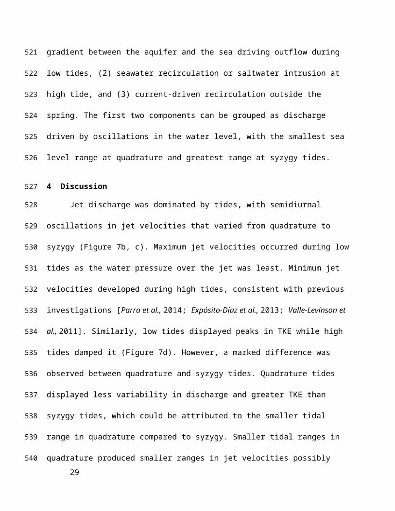
Jet discharge was dominated by tides, with semidiurnal oscillations in jet velocities that
varied from quadrature to syzygy (Figure 7b, c). Maximum jet velocities occurred during low
tides as the water pressure over the jet was least. Minimum jet velocities developed during high
tides, consistent with previous investigations [Parra et al., 2014; Expósito-Díaz et al., 2013;
Valle-Levinson et al., 2011]. Similarly, low tides displayed peaks in TKE while high tides
damped it (Figure 7d). However, a marked difference was observed between quadrature and
syzygy tides. Quadrature tides displayed less variability in discharge and greater TKE than
syzygy tides, which could be attributed to the smaller tidal range in quadrature compared to
syzygy. Smaller tidal ranges in quadrature produced smaller ranges in jet velocities possibly
caused by the fast response of the aquifer to changes in water level. Therefore, an increase in
tidal range produced a subsequent increase in the jet velocity range.
4.1 Salt Intrusion
During high syzygy tides, reversals in jet velocity driven by tidal pumping were observed
from 25 July on to the end of the observation period (Figure 6c). These reversals were associated
with lagoon water flowing into the aquifer. Additionally, salinity and temperature signals at the
jet indicated warm and salty lagoon water entered the spring (concurrent with downward jet
velocities), which also confirmed the occurrence of salt intrusion at high tides (Figure 6d, e).
Instances of salt intrusion have also been observed at submarine springs discharging at the
northern Yucatan Peninsula coast [Valle-Levinson et al., 2011; Vera et al., 2012]. Valle-
Levinson et al., [2011] reported salt intrusion only during the highest water levels, therefore
attributing these cases to increased water pressure over the spring. However, the results in Puerto
Morelos lagoon suggested that the observed saltwater intrusion was caused by a more complex
relationship between tidal pumping and tidal amplitudes as explained below.
18
372
373
374
375
376
377
378
379
380
381
382
383
384
385
386
387
388
389
390
391
392
393
394
395

Flow reversals into the aquifer began on midday 25 July and continued through the end
of the time series (Figure 6c; dashed green line in Figure 6a). These flow reversals depended on
the hydraulic pressure gradient and density differences between the sea and aquifer [Valle-
Levinson et al., 2011]. This relationship can be approximated by using a modified form of the
Bernoulli equation that takes into account an energy balance of the system and includes frictional
losses, assuming the flow within the aquifer was comparable to pipe flow. The friction term
should be included because the flow within the aquifer’s conduits and cave formations is
considered turbulent [Bauer-Gottwein et al., 2011; Beddows et al., 2007]. The jet discharge, U2,
could be approximated as follows:
g ρ1 h1+ρ1 U1
2
2=g ρ2h2+
ρ2U 22
2+ρ jet hL (5)
This equation represents the energy (per unit volume) balance between a cenote (sinkholes) on
land (left hand side) and the submarine spring (right hand side). Friction losses within the
aquifer, hL (m2 s-2), could be defined using the Darcy-Weisbach equation [Okiishi et al., 2006] :
hL=fLU2
2
2 D(6)
where f is the friction factor estimated at 0.016, L is the distance between the cenote and spring
estimated at 2 km and D is the diameter of the spring opening estimated at 1 m. Assuming U 1 at
the cenote is negligible, an inland water level of h1 = 6 cm above sea level, a freshwater density
of ρ1 = 1000 kg m-3, lagoon water density of ρ2 = 1025 kg m-3, and using the sea level
oscillations over the jet as h2, then jet velocities are reasonably predicted by
U 22=
2 g (ρ1 h1−ρ2 h2)
ρ2(1+ fLD
)(7)
19
396
397
398
399
400
401
402
403
404
405
406
407
408
409
410
411
412
413
414
415

as observed in Figure 8b (r2=0.75). Negative velocities were assumed when the right hand side of
the equation became negative. The resulting hydraulic gradient of 30 mm km-1 (¿h1/ L) is within
ranges of 7-10 mm km-1 and 50-100 mm km-1 provided by Beddows et al., [2007] and González-
Herrera et al., [2002], respectively. Jet velocities for hydraulic gradients of 5 and 100 mm km-1
are also plotted, showing the expected discharge during dry and wet periods, respectively. The
dry period jet velocity estimates (red) show average outflow of 0.37 throughout with no periods
of salt intrusion. The wet period jet velocity estimates (green) show predominant salt intrusion
during most high tides, except at the peak of quadrature tides on day 22. This relationship for jet
velocities suggests that density differences, hydraulic gradient and friction losses play an
important role in the dynamics of the system. It also could be used to predict when jet flows
should reverse direction. However, the approximation underestimated the maximum intrusion jet
velocities during syzygy and overestimated them before the peak of neap tides. This suggested
other factors were affecting jet velocities. These factors include a dynamic aquifer water table or
density gradients (equation assumed these to be static), and unknown dynamics within the
aquifer caves and conduits, among others.
Although instantaneous jet velocities during low tides were stronger at syzygy than
quadrature, subtidal velocities were greater in quadrature than syzygy (dashed red line of Figure
6c). This is relevant because previous studies have observed greater SGD seepage discharge rates
in syzygy than in quadrature [Kim and Hwang, 2002; Taniguchi, 2002]. The different reaction
observed at Pargos spring could be attributed to the fact that point-source SGDs have faster
response times to changes in water surface than seepage SGD. Faster responses are caused by the
high hydraulic conductivity (describes water movement through soils) of the Yucatan aquifer
system [Valle-Levinson et al., 2011]. The response time of Pargos spring velocities, U , to
20
416
417
418
419
420
421
422
423
424
425
426
427
428
429
430
431
432
433
434
435
436
437
438

changes in the water surface, η, was 22 min as calculated with a cross-correlation of the two
data sets (r2=0.65). Similarly, Vera et al., [2012] measured the long-term variability of a coastal
karst aquifer in the northern Yucatan Peninsula and found high correlation and phase agreement
between sea level variations and spring discharge. Furthermore, lag times between coastal karst
aquifers and sea level have been studied, specifically during the passage of hurricanes [Vera et
al., 2012]. These authors observed reversals in the flow at a submarine spring in the northern
Yucatan coast during Hurricane Ike. Salt intrusion lasted 2 days as observed at a cenote or
sinkhole just 150 m from shore, and remained for 26 days at a well found 10 km inland. In
contrast, [Smith et al., 2008] observed the effects of the passage of two hurricanes on seepage
SGD on the Florida coast. The hurricanes produced a reversal in the hydraulic gradient that took
80-130 d to dissipate. The large difference between the two locations could be attributed, again,
to the greater hydraulic conductivity of the Yucatan’s aquifer system when compared to
Florida’s aquifer, even though both are of karstic origin.
Moreover, subtidal jet velocities were positive (outflow) throughout with the exception of
midday 28 July 2011 (Figure 6c), which coincided with the peak wave setup (Figure 6b, ~5 cm)
generated by the storm. This was noteworthy because it showed the great vulnerability of the
system to small changes in water level. An increase of only 5 cm in the water level dropped the
subtidal velocities from 8 cm s-1 to zero. Wave setup increased hydrostatic pressure over the
spring, which appeared to inhibit both the discharge and turbulence.
4.2 Turbulent Kinetic Energy (TKE)
Semidiurnal and fortnightly oscillations were also observed in the TKE time series
(Figure 7d). Peaks in the jet’s TKE became more intense as quadrature tides approached,
reaching maximum TKE on 23 July. Thereafter, TKE maxima progressively decreased as tidal
21
439
440
441
442
443
444
445
446
447
448
449
450
451
452
453
454
455
456
457
458
459
460
461

amplitudes increased, pointing to an inverse relationship between the TKE trend and tidal range.
The lowest values of TKE (0.001 m2 s-2) were observed during syzygy tides, suggesting that tidal
pumping during syzygy tides inhibited TKE growth from the jet discharge. Furthermore, wave-
induced setup could have inhibited TKE at the jet, as the greatest significant wave height
coincided with the peak of syzygy tides and the minimum TKE values. A setup of only 5 cm
reduced subtidal TKE by half. Therefore, TKE were primarily driven by semidiurnal tides, with
the tidal range and wave setup acting as a secondary drivers. An exponential equation to explain
the relationship between TKE and sea level variations was proposed by Parra et al., [2014] for a
3 day time series. However, their relationship does not explain the TKE pattern observed here
(r2=0.09) and even the best fit between TKE and water level was not reliable (r2=0.23). The
exponential relationship previously proposed would suggest greater TKE produced during
syzygy when the tidal range was greatest. Yet, TKE decreased with the approach of syzygy. This
suggests that TKE observed at the spring opening could be comprised of turbulence that was
locally-generated and advected from within the aquifer.
Flows in the conduits and caves of the Yucatan aquifer system are known to be
dominated by turbulence [Bauer-Gottwein et al., 2011; Beddows et al., 2007]. Generally,
turbulence is expected to be proportional to mean velocities. However, the maximum TKE at the
jet did not occur at maximum jet velocities (Figure 6c). Consequently, it is postulated that
turbulence intensity was driven by other factors. It could be assumed that the TKE observed at
the jet included two components: turbulence generated locally by jet velocities and turbulence
advected from within the aquifer system. Using this assumption, it can be expected that extended
periods of outflow would produce increasing levels of turbulence within the aquifer. In other
words, we could expect increased TKE when subtidal flows were greatest, and decreased TKE
22
462
463
464
465
466
467
468
469
470
471
472
473
474
475
476
477
478
479
480
481
482
483
484

when subtidal flows were least. This relationship was observed when comparing subtidal TKE
with subtidal jet velocities (Figure 6c). Additionally, maximum TKE on 22 July also coincided
with the minimum jet velocity range. The small jet velocity range produced steady flows within
the aquifer that allowed for the greatest growth of TKE. This explanation is analogous to the
system having “memory” of what previously happened. The “memory” of the aquifer is to
discharge water toward the ocean. The aquifer had the “memory” of previous cycles when
subtidal outflows were maximum (during quadrature), producing the subsequent buildup of
TKE. However, jet flows during syzygy were greatly influenced by pulses of inflow and by
minimum subtidal velocities. During syzygy the system appeared to have lost “memory” of
previous cycles as represented by weakened subtidal outflows and subtidal turbulence. Inflow
pulses effectively disrupted the “memory” of the aquifer. Turbulence within the aquifer is
relevant as it could increase the rate of chemical reactions between saltwater and the karstic
substrate [Clemens et al., 1997; Kaufmann and Braun, 1999; Moore, 1999]. These reactions
could alter the concentrations of nutrients that discharge into the lagoon and affect the coral reefs
and related ecosystems. Future efforts should consider these responses. Furthermore, increased
turbulence in the spring discharge could produce increase rates of mixing between jet and lagoon
waters that could dilute pollutants and increase the exchange rates between reefs and seawater
[Reidenbach et al., 2006].
4.3 Waves
Wind-waves are known to drive circulation within the Puerto Morelos lagoon [Enriquez
et al., 2012; Coronado et al., 2007]. Spectral energy of wind-generated waves observed at the
forereef and over the spring was mostly concentrated within the 0.1-0.3 Hz frequency range
throughout the time series (Figure 4c). Infragravity wave energy (<0.1 Hz) increased during
23
485
486
487
488
489
490
491
492
493
494
495
496
497
498
499
500
501
502
503
504
505
506
507
periods of higher significant wave heights (between 23-26, 28-30 July), and were of greater
relative energy over Pargos spring (Figure 5b) than at the forereef. Therefore, a link was
apparent between increased wave heights and infragravity wave enhancement observed at the
forereef. The presence of infragravity waves in the Puerto Morelos lagoon has been reported
numerically [Torres-Freyermuth et al., 2012]. According to them, these low-frequency pulses
were controlled by offshore wave energy and related to “nonlinear energy transfer from higher
frequencies.” Therefore, greater activity within the infragravity range was to be expected with
increased wave energy from wind forcing, as observed.
On the other hand, the spectral energy of the jet discharge (Figure 5d) was different from
that of the water level (Figure 5b). Jet velocity spectral energy varied with a semidiurnal pattern.
During quadrature tides, elevated spectral energy was observed at all frequencies (e.g., 22 July).
Syzygy tides, however, showed low spectral energy at the highest frequencies during high tides
(e.g., day 28), when the discharge reversed directions. Additionally, a band of high spectral
energy appeared within the wind-wave frequency range (around 0.1 Hz). This indicated that
wind-wave effects could have influenced the jet discharge during syzygy at high tides. Wind-
wave influence on jet discharge was corroborated with the squared-coherence between sea level
and jet discharge at Pargos spring (Figure 5e). Significant squared-coherence (>99 % confidence
limit, bold black contour line) was observed during the second half of the time series within the
0.01-0.3 Hz frequency range that included both wind-waves and infragravity waves. This
showed that waves indeed modulated the discharge through wave pumping. Such observation
can be explained by the fact that the periods of high coherence at the wind-wave and infragravity
frequencies occurred at high tides, when jet velocities had reversed (salt-intrusion). In these
cases, wave influence would be observed as the jet discharge became lagoon water flowing into
24
508
509
510
511
512
513
514
515
516
517
518
519
520
521
522
523
524
525
526
527
528
529
530

the aquifer. When the jet discharge reversed direction during high syzygy tides and 5 cm wave
setup, wind-waves and infragravity waves played a role in modulating the discharge through
wave pumping.
4.4 Jet Temperatures and Salinities
In addition to the effects of tides and waves on the jet discharge, tidal effects were
observed on the jet’s temperature and salinity (Figure 6d, e). Quadrature tides showed starkly
different temperature and salinity oscillations than syzygy tides. At the height of quadrature tides
throughout 22 July, jet temperatures and salinities were practically constant (~27.1 °C, ~29 g kg-
1). The rest of quadrature tides produced triangle-like peaks with sharp increases toward high
tides and more gradual decreases toward low tides. A similar triangular pattern was observed at
this jet in July 2010 [Parra et al., 2014]. In contrast, syzygy tides produced greater temperature
and salinity oscillations between high and low tides (up to 3 °C, 10 g kg-1) than quadrature tides
(≤1 °C, <4 g kg-1). Both temperature and salinity oscillations during syzygy tides exhibited a
rectangular shape with sharp increases as high tides approached, and sudden drops as low tides
were reached. During syzygy high tides, temperatures and salinities at the jet were nearly
equivalent to those observed at the lagoon bottom, suggesting seawater intrusion. Concurrently,
jet velocities were negative, showing flow of water from the lagoon into the aquifer. A similar
rectangular pattern was observed by Expósito-Díaz et al., [2013], although their jet temperatures
were warmer than the ambient during their measurement period (autumn in a mangrove lagoon
some 160 km south of Puerto Morelos) and flow reversals were not observed. Low tides
produced smoothly decreasing jet temperatures. Because the water temperature within the
aquifer remains ~25° C year-round, the decreasing jet temperatures indicated that discharging
spring waters originated from further inland within the aquifer. Inside the Yucatan aquifer
25
531
532
533
534
535
536
537
538
539
540
541
542
543
544
545
546
547
548
549
550
551
552
553

system, a trend of decreasing temperatures from the coast to inland has been previously observed
[Beddows et al., 2007]. However, low tides also displayed increasing jet salinities, which point to
increased mixing of aquifer and sea waters throughout the progression of low tides. These
seemingly contradicting patterns suggested that the jet conduit is connected to a stratified cave
within the aquifer with cool and salty water below cool and fresher waters (Figure 9), as
previously suggested by Parra et al. [2014]. As low tides approached, the first waters to
discharge were from the cool and fresher water layer on top (Figure 9a), corroborated by the
salinity minima observed at the start of outflow at every low tide after 25 July (Figure 6e). Then
as discharge continued, mixing between the two cave-layers increased, producing higher salinity
discharge (Figure 9b). Furthermore, because discharging waters originated from further within
the aquifer as low tide progressed, discharge temperatures also gradually decreased throughout
low tides. Therefore, this aquifer cave system has a vertical salinity gradient and a horizontal
temperature gradient. The Yucatan Peninsula aquifer system is karstic and highly hydraulically
conductive. Cave divers have mapped many miles of submerged caves and tunnels and have
discovered an abundance of stratified caves throughout [Beddows et al., 2007]. Additionally,
unpublished field data show a cavity in the aquifer of 30-50 m height that appears to connect to
Pargos spring (M. Rebolledo-Vieyra pers. comm.) and divers at Pargos have observed the jet
conduit spanning ~10 m, at which point the conduit opened into a large cave. Further fieldwork
is necessary in this particular area to produce more detailed topo-bathymetric and hydrographic
charts of the aquifer cave systems.
A stratified water column within the cave could be expected despite the turbulence
observed in the jet discharge and the inflow of lagoon waters. By considering conservation of
26
554
555
556
557
558
559
560
561
562
563
564
565
566
567
568
569
570
571
572
573
574
575

mass, Q=U1A1, the velocities created by the salt intrusion at the jet into the aquifer cave could be
ascertained.
U 1( π D12
4 )=U 2( π D22
4 ) (8)
U 1 D12=U 2 D2
2 (9)
The observed inflow of lagoon waters at the jet were of 0.2 m s-1 magnitude through an
opening of ~1 m diameter, into a cave of assumed diameter of 30 m would produce a velocity of
0.2 mm s-1 within the cave. These low cave velocities would allow the formation of a stratified
water column, as have been observed throughout the area [Beddows et al., 2007].
5 Conclusion
The jet discharge was primarily modulated by semidiurnal tides and explained by a
relationship including density gradients and hydraulic gradients between the aquifer and jet, and
frictional losses throughout the system. A wave setup of 5 cm within the lagoon reduced subtidal
jet velocities by 8 cm s-1 and subtidal TKE by half. The jet salinity and temperature readings
suggested that the jet conduit was connected to a stratified cave with fresher cool waters
overlaying saltier cool waters (Figure 9).
This expansion in our understanding of the connections between coastal karstic aquifers
and sea level modulations has particular implications for water resource protection. Not only
must we be concerned with the overuse of groundwater reserves, but we should consider how
rising sea levels can also adversely affect this valuable resource. However, rising seas in
conjunction with storm events and syzygy tides can potentially pollute coastal aquifers within a
shorter time scale than previously expected. Additionally, the dynamics of these spring
discharges also have implications for the coastal ecosystems of the area. Therefore, further
27
576
577
578
579
580
581
582
583
584
585
586
587
588
589
590
591
592
593
594
595
596
597

studies are needed to understand these systems through longer temporal scales and including
remote forcing such as variations outside the lagoon in the Yucatan Current.
REFERENCES
Baas, A. C. (2006), Wavelet power spectra of aeolian sand transport by boundary layer
turbulence, Geophys. Res. Lett., 33(5).
Bakhtyar, R., D. A. Barry, and A. Brovelli (2012), Numerical experiments on interactions
between wave motion and variable-density coastal aquifers, Coast. Eng., 60, 95-108.
Bauer-Gottwein, P., B. R. Gondwe, G. Charvet, L. E. Marín, M. Rebolledo-Vieyra, and G.
Merediz-Alonso (2011), Review: The Yucatán Peninsula karst aquifer, Mexico, Hydrogeol.
J., 19(3), 507-524.
Beddows, P. A., P. L. Smart, F. F. Whitaker, and S. L. Smith (2007), Decoupled fresh–saline
groundwater circulation of a coastal carbonate aquifer: spatial patterns of temperature and
specific electrical conductivity, Journal of Hydrology, 346(1), 18-32.
Bricker, J. D. and S. G. Monismith (2007), Spectral wave-turbulence decomposition, J. Atmos.
Ocean. Technol., 24(8), 1479-1487.
Carretero, S., J. Rapaglia, H. Bokuniewicz, and E. Kruse (2013), Impact of sea-level rise on
saltwater intrusion length into the coastal aquifer, Partido de La Costa, Argentina, Cont.
Shelf Res., 61, 62-70.
Chérubin, L., C. Kuchinke, and C. Paris (2008), Ocean circulation and terrestrial runoff
dynamics in the Mesoamerican region from spectral optimization of SeaWiFS data and a
high resolution simulation, Coral Reefs, 27(3), 503-519.
28
598
599
600
601
602
603
604
605
606
607
608
609
610
611
612
613
614
615
616
617
618
619
Clemens, T., D. Hueckinghaus, M. Sauter, R. Liedl, and G. Teutsch (1997), Modelling the
genesis of karst aquifer systems using a coupled reactive network model, IAHS
PUBLICATION(241), 3-10.
Coronado, C., J. Candela, R. Iglesias-Prieto, J. Sheinbaum, M. López, and F. Ocampo-Torres
(2007), On the circulation in the Puerto Morelos fringing reef lagoon, Coral Reefs, 26(1),
149-163.
Emery, W. J. and R. E. Thomson (2001), - Data Analysis Methods in Physical Oceanography,
1st ed., Elsevier.
Enriquez, C., I. Mariño-Tapia, A. Valle-Levinson, A. Torres-Freyermuth, and R. Silva-Casarín
(2012), Mechanisms driving the circulation in a fringing reef lagoon: a numerical study,
Book of Abstracts of the Physics of Estuaries and Coastal Seas Symposium.
Expósito-Díaz, G., M. A. Monreal‐Gómez, A. Valle‐Levinson, and D. A. Salas‐de‐León (2013),
Tidal variations of turbulence at a spring discharging to a tropical estuary, Geophys. Res.
Lett., 40(5), 898-903.
Ferguson, G. and T. Gleeson (2012), Vulnerability of coastal aquifers to groundwater use and
climate change, Nature Climate Change, 2(5), 342-345.
Fitterman, D. V. (2014), Mapping Saltwater Intrusion in the Biscayne Aquifer, Miami-Dade
County, Florida using Transient Electromagnetic Sounding, Journal of Environmental and
Engineering Geophysics, 19(1), 33-43.
Fleury, P., M. Bakalowicz, and G. de Marsily (2007), Submarine springs and coastal karst
aquifers: a review, Journal of Hydrology, 339(1), 79-92.
Gonneea, M. E., A. E. Mulligan, and M. A. Charette (2013), Climate‐driven sea level anomalies
modulate coastal groundwater dynamics and discharge, Geophys. Res. Lett., 40(11), 2701-
2706.
29
620
621
622
623
624
625
626
627
628
629
630
631
632
633
634
635
636
637
638
639
640
641
642
643

González-Herrera, R., I. Sánchez-y-Pinto, and J. Gamboa-Vargas (2002), Groundwater-flow
modeling in the Yucatan karstic aquifer, Mexico, Hydrogeol. J., 10(5), 539-552.
Grinsted, A., J. C. Moore, and S. Jevrejeva (2004), Application of the cross wavelet transform
and wavelet coherence to geophysical time series, Nonlinear processes in geophysics,
11(5/6), 561-566.
Hamner, W. W. and E. E. Wolanski (1988), Hydrodynamic forcing functions and biological
processes on coral reefs: a stus review, Proceedings of the 6th International Coral Reef
Symposium, Townsville, Australia 8-12 August 1988-pages: 1: 103-113.
Hu, C., F. E. Muller‐Karger, and P. W. Swarzenski (2006), Hurricanes, submarine groundwater
discharge, and Florida's red tides, Geophys. Res. Lett., 33(11).
Kang, S. and H. Lin (2007), Wavelet analysis of hydrological and water quality signals in an
agricultural watershed, Journal of Hydrology, 338(1), 1-14.
Kaufmann, G. and J. Braun (1999), Karst aquifer evolution in fractured rocks, Water Resour.
Res., 35(11), 3223-3238.
Kim, G. and D. Hwang (2002), Tidal pumping of groundwater into the coastal ocean revealed
from submarine 222Rn and CH4 monitoring, Geophys. Res. Lett., 29(14), 23-1-23-4.
Li, L., D. Barry, F. Stagnitti, and J. Parlange (1999), Submarine groundwater discharge and
associated chemical input to a coastal sea, Water Resour. Res., 35(11), 3253-3259.
McLachlan, A. and I. Turner (1994), The interstitial environment of sandy beaches, Mar. Ecol.,
15(3‐4), 177-212.
Merino, M., S. Czitrom, E. Jordán, E. Martin, P. Thomé, and O. Moreno (1990), Hydrology and
rain flushing of the Nichupté lagoon system, Cancún, Mexico, Estuar. Coast. Shelf Sci.,
30(3), 223-237.
30
644
645
646
647
648
649
650
651
652
653
654
655
656
657
658
659
660
661
662
663
664
665
666
Metcalfe, C. D., P. A. Beddows, G. G. Bouchot, T. L. Metcalfe, H. Li, and H. Van Lavieren
(2011), Contaminants in the coastal karst aquifer system along the Caribbean coast of the
Yucatan Peninsula, Mexico, Environmental pollution, 159(4), 991-997.
Millero, F. J., R. Feistel, D. G. Wright, and T. J. McDougall (2008), The composition of
Standard Seawater and the definition of the Reference-Composition Salinity Scale, Deep
Sea Research Part I: Oceanographic Research Papers, 55(1), 50-72.
Monismith, S. G. (2010), Mixing in estuaries, Contemporary Issues in Estuarine Physics, edited
by: Valle-Levinson, A, Cambridge University Press, Cambridge, 145-185.
Moore, W. S. (1996), Large groundwater inputs to coastal waters revealed by 226Ra
enrichments, Nature, 380(6575), 612-614.
Moore, W. S. (1999), The subterranean estuary: a reaction zone of ground water and sea water,
Mar. Chem., 65(1), 111-125.
Moore, W. S. (2010), The effect of submarine groundwater discharge on the ocean, Annual
review of marine science, 2, 59-88.
Null, K. A., K. L. Knee, E. D. Crook, N. R. de Sieyes, M. Rebolledo-Vieyra, L. Hernández-
Terrones, and A. Paytan (2014), Composition and fluxes of submarine groundwater along
the Caribbean coast of the Yucatan Peninsula, Cont. Shelf Res., 77, 38-50.
Okiishi, M. Y., B. Munson, and D. Young (2006), Fundamentals of Fluid Mechanics, John
Wiley & Sons, Inc.
Parra, S., I. Mariño-Tapia, C. Enriquez, and A. Valle-Levinson (2014), Variations in turbulent
kinetic energy at a point-source submarine groundwater discharge in a reef lagoon, Ocean
Dynamics.
Patterson, M. R., K. P. Sebens, and R. R. Olson (1991), In situ measurements of flow effects on
primary production and dark respiration in reef corals., Limnol. Oceanogr., 36(3), 936-948.
31
667
668
669
670
671
672
673
674
675
676
677
678
679
680
681
682
683
684
685
686
687
688
689
690
Peterson, R. N., W. C. Burnett, C. R. Glenn, and A. G. Johnson (2009), Quantification of point-
source groundwater discharges to the ocean from the shoreline of the Big Island, Hawaii,
Limnol. Oceanogr., 54(3), 890-904.
Pope, S. B. (2000), Turbulent Flows, Cambridge university press.
Precht, E. and M. Huettel (2003), Advective pore-water exchange driven by surface gravity
waves and its ecological implications, Limnol. Oceanogr., 48(4), 1674-1684.
Reidenbach, M. A., S. G. Monismith, J. R. Koseff, G. Yahel, and A. Genin (2006), Boundary
layer turbulence and flow structure over a fringing coral reef, Limnol. Oceanogr., 51(5),
1956.
Santos, I. R., W. C. Burnett, J. Chanton, N. Dimova, and R. N. Peterson (2009), Land or ocean?:
Assessing the driving forces of submarine groundwater discharge at a coastal site in the Gulf
of Mexico, Journal of Geophysical Research: Oceans (1978–2012), 114(C4).
Santos, I. R., F. Niencheski, W. Burnett, R. Peterson, J. Chanton, C. F. Andrade, I. B. Milani, A.
Schmidt, and K. Knoeller (2008), Tracing anthropogenically driven groundwater discharge
into a coastal lagoon from southern Brazil, Journal of Hydrology, 353(3), 275-293.
Smith, C. G., J. E. Cable, and J. B. Martin (2008), Episodic high intensity mixing events in a
subterranean estuary: Effects of tropical cyclones, Limnol. Oceanogr., 53(2), 666.
Taniguchi, M. (2002), Tidal effects on submarine groundwater discharge into the ocean,
Geophys. Res. Lett., 29(12), 2-1-2-3.
Taniguchi, M., W. C. Burnett, J. E. Cable, and J. V. Turner (2002), Investigation of submarine
groundwater discharge, Hydrol. Process., 16(11), 2115-2129.
Torrence, C. and G. P. Compo (1998), A practical guide to wavelet analysis, Bull. Am. Meteorol.
Soc., 79(1), 61-78.
32
691
692
693
694
695
696
697
698
699
700
701
702
703
704
705
706
707
708
709
710
711
712
713

Torres-Freyermuth, A., I. Marino-Tapia, C. Coronado, P. Salles, G. Medellín, A. Pedrozo-
Acuna, R. Silva, J. Candela, and R. Iglesias-Prieto (2012), Wave-induced extreme water
levels in the Puerto Morelos fringing reef lagoon, Natural Hazards and Earth System
Science, 12(12), 3765-3773.
Uchiyama, Y., K. Nadaoka, P. Rölke, K. Adachi, and H. Yagi (2000), Submarine groundwater
discharge into the sea and associated nutrient transport in a sandy beach, Water Resour.
Res., 36(6), 1467-1479.
Valle-Levinson, A., I. Marino-Tapia, C. Enriquez, and A. F. Waterhouse (2011), Tidal variability
of salinity and velocity fields related to intense point-source submarine groundwater
discharges into the coastal ocean, Limnol. Oceanogr., 56(4), 1213-1224.
Vera, I., I. Mariño-Tapia, and C. Enriquez (2012), Effects of drought and subtidal sea-level
variability on salt intrusion in a coastal karst aquifer, Marine and Freshwater Research,
63(6), 485-493.
Werner, A. D. and C. T. Simmons (2009), Impact of sea‐level rise on sea water intrusion in
coastal aquifers, Groundwater, 47(2), 197-204.
Zektser, I. S. and L. G. Everett (2000), Groundwater and the Environment: Applications for the
Global Community, CRC Press.
33
714
715
716
717
718
719
720
721
722
723
724
725
726
727
728
729
730
731
732

Figure 1. Chart of the Puerto Morelos fringing coral reef lagoon on the eastern Yucatan
Peninsula of Mexico. Circle represents the location of Pargos spring where the Nortek Vector
and CTD were moored, squares represent the locations of the Nortek Vector at the forereef and
of the CTD within the lagoon, and the ‘X’ represents the meteorological station where winds
were recorded (depth and scale in meters).
34
733
734
735
736
737
738
739

Figure 2. Mean precipitation at nearest station in Cancun, Mexico (~30 km north of Puerto
Morelos). Data provided by Meteorological Assimilation Data Ingest System (MADIS) at
National Oceanic and Atmospheric Administration (NOAA).
35
740
741
742
743
744

Figure 3. Schematic of bathymetry at spring opening with approximate dimensions. Triangle
denotes location of ADV and CT moorings. The ADV was moored at the center of the vent (~7
m depth) with downward orientation. The CT was located about 25 cm above the sampling
volume of the ADV, both within the core or outflow.
36
745
746
747
748
749
Figure 4. Winds and waves at Puerto Morelos lagoon. (a) Hourly wind velocity vectors (blue),
and east (black) and north (red) wind components measured at the meteorological station,
showing the direction the wind was blowing; (b) significant wave heights, Hs, (blue) and peak
wave periods (green) at the forereef; and (c) spectral density of the water level bursts at the
forereef.
37
750
751
752
753
754
755

Figure 5. (a) Time series and (b) spectral contours of the hourly sea level bursts at Pargos
spring; (c) time series and (d) spectral contours of the hourly spring discharge velocities; and (e)
squared-coherence spectra between the sea level variations at Pargos and spring discharge bursts,
with the black line representing the 99 % confidence limit. The two black dashed lines represent
instances of peak high and low tides.
38
756
757
758
759
760
761
762
Figure 6. (a) Sea level variations at Pargos (blue) and the forereef (red), the dashed green line
represents the high tide observed during the first flow reversal event on day 25.5; (b) setup (blue)
and significant wave heights (blue) observed at the jet; (c) TKE (blue) and jet discharge
velocities (red) at the jet opening, with the dashed lines representing 30-hour low-pass filter and
the dotted line representing the zero velocity value; (d) temperatures at the jet (blue) and the
lagoon bottom (black); and (e) salinities at the jet (blue) and the lagoon bottom (black). The
black dashed lines represent instances of peak high and low tides.
39
763
764
765
766
767
768
769

Figure 7. Wavelet and time series of significant wave heights (a) at the forereef; (b) water
level at the jet; (c) jet vertical velocities; and (d) TKE at the jet. In the wavelet plots, shaded
regions on both bottom corners indicate the cone of influence, where edge effects become
important and data is less reliable. The bold black contours in wavelet plots encircle regions of
>95 % confidence.
40
770
771
772
773
774
Figure 8. (a) Sea level variations at Pargos spring and (b) actual (bold, black) and estimated jet
discharge velocities for varying hydraulic conductivities: 5 mm km-1(green), 30 mm km-1(blue)
and 100 mm km-1(red). The dotted black line represents the zero velocity mark.
41
775
776
777
778
779

Figure 9. Schematic of proposed aquifer cave system at the (a) start and (b) middle of low
tides in syzygy. The dashed line represents the halocline or interphase between the two water
layers.
42
780
781
782
783
784