Low frequency modes on

two fringing reefs:

Observations & dynamics

A THESIS SUBMITTED TO

THE GLOBAL ENVIRONMENTAL SCIENCE

UNDERGRADUATE DIVISION IN PARTIAL FULFILLMENT

OF THE REQUIREMENTS FOR THE DEGREE OF

Bachelor of Science

in

Global Environmental Science

May 2013

By:

Hyang Yoon

Thesis Advisor:

Janet M. Becker

I certify that I have read this thesis and that, in my opinion, it is

satisfactory in scope and quality as a thesis for the degree of Bachelor

of Science in Global Environmental Science.

Thesis Advisor

Janet M. Becker

Department of Geology & Geophysics

ii

Dedicated to my grandfather

Dr. Jong Teck Kim

October 1929 – December 2010

iii

ACKNOWLEDGMENTS

First and foremost, I would like to express my sincere gratitude to my thesis advisor Janet

Becker for her continuous support, patience, motivation, enthusiasm and extensive knowl-

edge. Her guidance helped me throughout my research and while writing this thesis. I

could not have imagined having a better advisor and mentor for my studies. Besides my

advisor, I would also like to thank all the other professors and staff in the School of Ocean

and Earth Science and Technology. Especially Mark Merrifield for helping me create the

codes that were vital to my research, for his encouragement and for his generous support.

I would also like to thank NSF who funded the research and to the group that set up

and collected the data for this study. If not for these supporters, this research would not

have been possible. My sincere thanks goes to Ricky Fong’s family for supporting my study

through the Ricky Chi Kan Fong Memorial Scholarship. Being an international student is

not easy and their support helped me achieve where I am today.

I send my thanks to my fellow GES members for the stimulating discussions, for the

stress we shared and for all the fun we have had together. I thank my friends, spread all

over the world, for their continuous support. I also thank my second family in Hawai‘i, the

people of the Ohnishi residence. Thank you for supporting me from the first day I arrived

on this island and for providing me a home, miles away from Japan.

Last but not the least, I would like to thank my own family. Especially my parents,

TaeHo Yoon and HyangJa Kim, for supporting me unconditionally throughout my life, and

my older brother Seob Yoon for introducing me to Hawai‘i and, thus, making it possible for

me to study at the University of Hawai‘i at Manoa.

iv

ABSTRACT

Surface gravity waves are an important physical feature of the ocean that affect nearshore

processes, such as coastal inundation. Wave driven inundation results from increased coastal

water levels due to high and low frequency waves, breaking wave set-up and the tide. To

understand and predict wave driven inundation over a fringing reef, it is necessary to relate

incident wave conditions to the response at the coast. In this study, we focus on observations

and dynamics of the high and low frequency waves. Bottom pressure measurements across

two fringing coral reefs in the Republic of the Marshall Islands are analyzed in an effort to

relate incident wave energy measured on the fore reef to the energy at the shoreline. Time

series of significant wave height in the high and low frequency bands are examined, and the

records with large wave energy are identified and analyzed spectrally. The largest observed

shoreline response is due to low frequency motions on the reef flat. Spectral peaks during

the largest events occurred at a period T0 = 4L/√gh which is consistent with the excitation

of a quarter wave length normal mode on the reef flat. The amplitude of this normal mode

increases shoreward leading to enhanced low frequency energy at the shoreline.

v

TABLE OF CONTENTS

Acknowledgments . . . . . . . . . . . . . . . . . . . . . . . . . . . . . . . . . . . . iv

Abstract . . . . . . . . . . . . . . . . . . . . . . . . . . . . . . . . . . . . . . . . . . v

List of Tables . . . . . . . . . . . . . . . . . . . . . . . . . . . . . . . . . . . . . . . viii

List of Figures . . . . . . . . . . . . . . . . . . . . . . . . . . . . . . . . . . . . . . ix

List of Abbreviations and Symbols . . . . . . . . . . . . . . . . . . . . . . . . . xi

Chapter 1 Introduction . . . . . . . . . . . . . . . . . . . . . . . . . . . . . . . . 1

1.1 Infragravity Wave Field Studies . . . . . . . . . . . . . . . . . . . . . . . . . 4

1.2 Laboratory Experiments . . . . . . . . . . . . . . . . . . . . . . . . . . . . . 5

1.3 Numerical Modeling . . . . . . . . . . . . . . . . . . . . . . . . . . . . . . . 6

1.4 Alternative Views . . . . . . . . . . . . . . . . . . . . . . . . . . . . . . . . . 7

Chapter 2 Site Description . . . . . . . . . . . . . . . . . . . . . . . . . . . . . 8

Chapter 3 Data . . . . . . . . . . . . . . . . . . . . . . . . . . . . . . . . . . . . . 10

Chapter 4 Methods . . . . . . . . . . . . . . . . . . . . . . . . . . . . . . . . . . 12

4.1 Wave Characteristics and Properties . . . . . . . . . . . . . . . . . . . . . . 12

4.2 Dispersion Relation . . . . . . . . . . . . . . . . . . . . . . . . . . . . . . . . 13

4.3 Data Processing . . . . . . . . . . . . . . . . . . . . . . . . . . . . . . . . . 15

4.4 Free Surface Elevation . . . . . . . . . . . . . . . . . . . . . . . . . . . . . . 16

4.5 Significant Wave Height . . . . . . . . . . . . . . . . . . . . . . . . . . . . . 19

4.6 Band Pass Filter . . . . . . . . . . . . . . . . . . . . . . . . . . . . . . . . . 20

4.7 Auto Spectrum . . . . . . . . . . . . . . . . . . . . . . . . . . . . . . . . . . 22

4.8 Lower Frequency Limit . . . . . . . . . . . . . . . . . . . . . . . . . . . . . . 23

vi

Chapter 5 Time Domain Analysis . . . . . . . . . . . . . . . . . . . . . . . . . 24

5.1 Cross Shore Transformation . . . . . . . . . . . . . . . . . . . . . . . . . . . 24

5.2 Significant Wave Height . . . . . . . . . . . . . . . . . . . . . . . . . . . . . 25

Chapter 6 Wave Dynamics . . . . . . . . . . . . . . . . . . . . . . . . . . . . . 33

6.1 Long Wave Equations: Normal Modes . . . . . . . . . . . . . . . . . . . . . 33

Chapter 7 Spectral Analysis . . . . . . . . . . . . . . . . . . . . . . . . . . . . . 36

7.1 Cross Shore Transformation . . . . . . . . . . . . . . . . . . . . . . . . . . . 36

7.2 Effect of Water Level . . . . . . . . . . . . . . . . . . . . . . . . . . . . . . . 39

7.3 Effect of Reef Length . . . . . . . . . . . . . . . . . . . . . . . . . . . . . . . 42

7.4 Reef Flat Transformation . . . . . . . . . . . . . . . . . . . . . . . . . . . . 46

Chapter 8 Discussion . . . . . . . . . . . . . . . . . . . . . . . . . . . . . . . . . 49

Appendix A Band Width . . . . . . . . . . . . . . . . . . . . . . . . . . . . . . 52

Appendix B Peak Period Errors . . . . . . . . . . . . . . . . . . . . . . . . . . 54

References . . . . . . . . . . . . . . . . . . . . . . . . . . . . . . . . . . . . . . . . . 58

vii

LIST OF TABLES

Table Page

3.1 Information on the reef profile and sensors used in this research . . . . . . . 10

4.1 Definition of shallow, intermediate and deep water limits . . . . . . . . . . . 14

5.1 High energy events observed at ROI and CMI . . . . . . . . . . . . . . . . . 26

7.1 Observed peak frequency and period compared with the theoretical peak period 40

7.2 Observed peak frequency and period compared with the theoretical peak period 44

A.1 Adjusted band width . . . . . . . . . . . . . . . . . . . . . . . . . . . . . . . 52

B.1 Observed period versus theoretical period at ROI . . . . . . . . . . . . . . . 55

B.2 Observed period versus theoretical period at CMI . . . . . . . . . . . . . . . 56

viii

LIST OF FIGURES

Figure Page

2.1 Map of the Republic of the Marshall Islands . . . . . . . . . . . . . . . . . . 8

2.2 Aerial view of ROI and CMI . . . . . . . . . . . . . . . . . . . . . . . . . . 9

3.1 Reef profile and sensor location of ROI and CMI . . . . . . . . . . . . . . . 11

4.1 Wave properties . . . . . . . . . . . . . . . . . . . . . . . . . . . . . . . . . . 12

4.2 Difference of water particle orbits in deep and shallow water . . . . . . . . . 15

4.3 Pressure response factor . . . . . . . . . . . . . . . . . . . . . . . . . . . . . 17

4.4 Cross shore transition of the free surface elevation at ROI and CMI . . . . . 18

4.5 Significant wave height vs time . . . . . . . . . . . . . . . . . . . . . . . . . 19

4.6 A box car band pass filter . . . . . . . . . . . . . . . . . . . . . . . . . . . . 21

4.7 Cross shore transformation of free surface elevation in SS and IG . . . . . . 22

5.1 Free surface elevation at ROI in SS and IG . . . . . . . . . . . . . . . . . . 25

5.2 Significant wave height at ROI . . . . . . . . . . . . . . . . . . . . . . . . . 27

5.3 Significant wave height at CMI . . . . . . . . . . . . . . . . . . . . . . . . . 28

5.4 Scatter plots of SS wave heights at the shoreline sensor vs the mid reef sensor 30

5.5 Scatter plots of shoreline SS wave heights versus local water level . . . . . . 31

5.6 Scatter plots of IG waves over the reef flat sensors . . . . . . . . . . . . . . 32

6.1 Standing wave in an idealized reef . . . . . . . . . . . . . . . . . . . . . . . 34

7.1 Spectral density of cross shore transformation of wave energy . . . . . . . . 38

7.2 Effect of water level to the peak frequency at ROI and CMI . . . . . . . . . 41

ix

7.3 Effect of reef length on peak frequency . . . . . . . . . . . . . . . . . . . . . 45

7.4 Auto spectra at ROI 1 and ROI 3 for four time series . . . . . . . . . . . . 47

7.5 Auto spectra at CMI 2 and CMI 4 for four time series . . . . . . . . . . . . 48

8.1 Free surface elevation of sea and swell and envelope . . . . . . . . . . . . . . 51

A.1 Differences (Original–(a),(b), or original) . . . . . . . . . . . . . . . . . . . . 53

x

LIST OF ABBREVIATIONS AND SYMBOLS

a Amplitude

CMI Short for College of the Marshall Islands at Majuro Atoll

CMI 2 Sensor 2 on the reef flat at CMI

CMI 4 Sensor 4 on the reef flat at CMI

CMI 7 Sensor 7 one the fore reef at CMI

η Free surface elevation

f Frequency (inverse of the period, 1/T )

fn Modal frequency, where n are non-negative integers

(inverse of the modal period, 1/Tn)

g Gravitation acceleration (9.81 m/s2)

h Water depth/water level

H Wave height

Hz Hertz

IG Infragravity (low frequency)

k Wave number

Kp Pressure response factor

L Cross shore length of the reef flat

λ Wavelength

m Meters

min Minutes

ω Angular frequency (2πf)

P Bottom pressure

ρ Density of water

ROI Short for Roi-Namur at Kwajalein Atoll

ROI 1 Sensor 1 on the reef flat at ROI

ROI 3 Sensor 3 on the reef flat at ROI

ROI 5 Sensor 5 on the fore reef at ROI

sec (or s) Seconds

SS Sea and swell (high frequency)

T Period (inverse of the frequency, 1/f)

Tn Modal period, where n are non-negative integers

(inverse of the modal frequency, 1/fn)

x Cross shore distance

xi

CHAPTER 1: INTRODUCTION

Surface gravity waves are an important physical feature of the ocean that affect nearshore

processes and contribute to coastal inundation. Fringing reefs protect the shoreline by

dissipating wave energy through breaking at the fore reef and additionally through frictional

effects and breaking over the reef flat. Reef fringed islands and atolls, for example the

Okinawa Islands, Guam and the Republic of the Marshall Islands, have been threatened by

inundation due to ocean waves during storm events.

In 1987, a typhoon passing near the Okinawa Islands in Japan caused great coastal

damage due to the rise of the water level from a bore-like surf beat (Nakaza et al., 1990).

When the waves hit the Okinawa Islands, the waves were more than 5 m higher than normal

conditions, damaging the land area near the shoreline (Nakaza et al., 1990). Nakaza et al.

(1990) related their observations to the excitation of the quarter-wavelength normal mode

on the reef flat. Previously, the coral reefs where thought to protect the island from wave

energy, which was been proven otherwise from this 1987 typhoon event at the Okinawa

Islands.

In 1979, near the Republic of the Marshall Islands a high pressure system was generated,

causing the sea level to rise above normal conditions. This also generated storm surge,

causing the sea level to rise over 6 m, resulting in an inundation evert on the East coast of

Majuro Atoll (Spennemann, 1998). This event caused injuries, damage of property, damage

of the sewage infrastructure causing approximately 30 million dollars of damage and having

nearly 5000 people to be relocated (Spennemann, 1998).

1

There was a potential wave driven inundation event in 2008 at the Republic of the

Marshall Islands (Ford et al., n.d.). Unlike the inundation event in 1979, less injuries were

reported. Nevertheless, 300 people were relocated due to the damage of properties (Ford

et al., n.d.). Damages are thought to be limited due to the low tidal levels during this event

(Ford et al., n.d.).

While inundation may occur from different factors including atmospheric disturbances,

this research is focused on wave driven inundation, which occurs when four components

of the ocean wave field add up to exceed the land elevation. The four components are:

high frequency waves (sea and swell), low frequency waves (infragravity), set-up and the

tide. Low lying lands are vulnerable to wave driven inundation since small changes in the

water level may result in inundation as seen in the Okinawa Islands and the Republic of

the Marshall Islands.

The tidal component of the wave driven inundation is as predictable as the tides are

due to astronomical forcing with well understood and predictable patterns. The setup is

the increase of mean water level due to the breaking of the high frequency waves. Setup

on the reef flat is known to decrease during high tide (Gourlay , 1996; Vetter et al., 2010),

therefore, setup and the tide oppose each other. The elevation of water on the reef flat

may be dominated by the setup, as seen during tropical storm Man-Yi over the Ipan reef,

Guam (Pequignet et al., 2009). High frequency waves are the waves that people surf and

this component on the reef flat is highly correlated with the local water level. The higher

the water level on the reef flat, the more high frequency energy is observed on the reef

flat (Vetter et al., 2010). Finally the low frequency wave component may be thought of as

2

the sets or groups of waves that people surf. The low frequency component of wave driven

inundation is the topic of this research and will be analyzed in this study.

Field studies and laboratory experiments have been conducted to better understand

surface waves and their transformation over reefs (e.g., Nakaza et al., 1990; Nakaza and

Hino, 1991; Gourlay , 1996; Pequignet et al., 2009; Nwogu and Demirbilek , 2010; Vetter

et al., 2010; Pomeroy et al., 2012; Pequignet et al., 2011; Van Dongeren et al., 2013).

Reefs of different forms, lengths, widths and reef flat water depths have been examined

in these studies. There have been studies that have focused on the breaking wave setup

(e.g., Gourlay , 1996; Nwogu and Demirbilek , 2010; Vetter et al., 2010; Van Dongeren et al.,

2013) and also the high frequency component of the waves, also known as sea and swell

waves (Pequignet et al., 2011). There also have been studies that focus on low frequency

component of the waves, also known as infragravity waves (e.g., Nakaza et al., 1990; Nakaza

and Hino, 1991; Pequignet et al., 2009; Nwogu and Demirbilek , 2010; Van Dongeren et al.,

2013). Prior studies have found that the infragravity waves may be due to the excitation

of a quarter-wavelength normal mode over the reef depending on the local water level.

The fringing reefs that have been researched in the past often have a lagoon between the

reef flat and the shoreline (Nwogu and Demirbilek , 2010; Pomeroy et al., 2012; Van Dongeren

et al., 2013). In contrast, for Okinawa, Japan studied by Nakaza et al. (1990) and Ipan,

Guam studied by Pequignet et al. (2009) the reefs are directly attached to the shoreline.

This research focuses on the study of infragravity waves and their dynamics over fringing

reefs in the Republic of the Marshall Islands directly attached to the shoreline similar to

the studies of Nakaza et al. (1990) and Pequignet et al. (2009).

3

1.1 INFRAGRAVITY WAVE FIELD STUDIES

Amplification of infragravity waves has been described in terms of open basin normal modes,

related to those that are observed over coastal shelves (Lugo-Fernandez et al., 1998). Lugo-

Fernandez et al. (1998) documented observations of an open basin normal mode over a

coastal shelf of 6 km long, on the Tague reef in St. Croix. Lugo-Fernandez et al. (1998)

concluded from their observations that the quarter-wavelength normal mode is dominant

on continental shelves.

Nakaza et al. (1990) spectrally analyzed pressure observations over a reef in the Okinawa

Islands during a typhoon event and found a distinctive peak in the low frequency spectrum

near the shore. They related this signal to the excitation of the quarter-wavelength normal

mode on the reef flat excited by the incident wave groups.

Pequignet et al. (2009) present results from a field study on Ipan reef, an approximately

450 m long fringing reef, on the southeast coast of Guam. This study demonstrated the

existence of low frequency modes on the reef during a large wave event due to tropical storm

Man-Yi. These modes are not observed on Ipan reef at normal water levels of approximately

0.5 m. Pequignet et al. (2009) observed amplification of infragravity waves, as the breaking

wave setup increased the water level to approximately 2.0 m over the reef. The increased

water depth became the key to the amplified infragravity waves during this wave events.

Nakaza et al. (1990) and Pequignet et al. (2009) concluded from their observations

that the quarter-wavelength normal mode is dominant on the fringing reef under storm

conditions. The quarter-wavelength modal period to which they refer follows the open

4

basin normal modes and is given by T0 = 4L/√gh, where L is the reef length (cross shore),

h is the water depth, and g is the gravitational acceleration (9.81 m/s2). This equation

shows that the modal period depends on the geometry of the reef and the water depth over

the reef.

1.2 LABORATORY EXPERIMENTS

Nakaza et al. (1990) also carried out laboratory experiments in addition to the observa-

tions made at the Okinawa Islands described above. Nakaza and Hino (1991) reported

experiments on a reef flat 4.2 m long, and water depth of 0.04 m. By generating irregular

incident wave events, Nakaza et al. (1990) found that the experimental modes observed

were consistent with the theoretical modes with period T0 = 4L/√gh.

Gourlay (1996) studied the setup of waves experimentally by creating idealized reefs

comparable to real reefs that are found world wide. In this study, Gourlay (1996) found

that, the setup increases as the water level on the reef decreases. There was one exception

however, on the idealized Guam reef when comparing regular and irregular incident waves

in the experiment. The idealized Male reef showed good agreement of submergence and

relative setup when comparing the regular and irregular wave events. However, Gourlay

(1996) found that the regular and irregular wave events did not agree for the idealized Guam

reef. Gourlay (1996) hypothesized that this disagreement was possibly due to the excitation

of the normal mode on the idealized reef which he did not account for his experiment.

Experiments performed by Nwogu and Demirbilek (2010) utilized a typical fringing reef

profile from Southeast Guam. Since the experimental setup was a wave flume, Nwogu and

5

Demirbilek (2010) were able to locate sensors at ideal locations and adjust the time the

sensors were in use. Nwogu and Demirbilek (2010) observed that infragravity energy was

low off shore and high on the reef flat. Moreover, the infragravity energy is documented to

be lowest at the reef crest and increased shoreward (Nwogu and Demirbilek , 2010). Nwogu

and Demirbilek (2010) spectrally analyzed the data by band averaging 30 frequencies to

increase the degrees of freedom and to increase the reliability of the data. Nwogu and

Demirbilek (2010) also analyzed the raw spectrum for maximum frequency resolution. The

raw spectrum for near shore sensors shows the highest infragravity energy at a period of 35

sec, which was consistent with the quarter-wavelength normal mode.

1.3 NUMERICAL MODELING

Recently, researchers have applied numerical models used for coastal shelfs on fringing reefs.

Along with the experimental study, Nwogu and Demirbilek (2010) also used a nonlinear

Boussinesq wave model to futher study wave transformation over a reef. The nonlinear

Boussinesq wave model was able to show that the infragravity energy was dominant at the

reef flat sensors. Nwogu and Demirbilek (2010) found that the model was consistent with the

observations made with their experimental setup, period of 35 sec, and they hypothesized

that the forcing of the infragravity waves could be due to the energy from the dissipation

of the short waves.

Van Dongeren et al. (2013) used the XBeach numerical model to understand the dynam-

ics of the infragravity waves at the Ningaloo reef in Western Australia. Analysis was done

both in a one-dimensional and two-dimensional domian. From this study, Van Dongeren

6

et al. (2013) found that for predicting the transformations of the infragravity waves, the

two-dimensional model was more accurate. From the model, Van Dongeren et al. (2013)

found that the amplitude of the infragravity waves are correlated with the water depth over

the reef flat. Moreover, the infragravity energy was dominant on the reef flat at Ningaloo

reef.

1.4 ALTERNATIVE VIEWS

Although much prior research supports the shelf resonance phenomena on the reef flat,

Pomeroy et al. (2012) did not see the same phenomena on the Ningaloo reef in Western

Australia. The Ningaloo reef is a fringing reef approximately 1.4 km long (Pomeroy et al.,

2012). While Pomeroy et al. (2012) found that the spectra on the reef flat was dominated

by infragravity energy, the observed infragravity wave energy energy was small even when

the incident wave was high. A shoreward increase in infragravity wave energy was not

observed. Rather, saw that the infragravity wave energy decreased as the wave propagated

over the reef flat (Pomeroy et al., 2012). The research by Pomeroy et al. (2012) shows that

normal modes are not observed over some reef flats, and that further study is necessary in

order to understand infragravity energy on the reef flat.

7

CHAPTER 2: SITE DESCRIPTION

The study site of this research is the Republic of the Marshall Islands, specifically two

atolls, Kwajalein Atoll and the Majuro Atoll (Figure 2.1). The Kwajalein array location

is referred to as ROI (short for Roi-Namur), and the Majuro array is referred to as CMI

(short for College of the Marshall Islands) throughout this research.

The fringing reef that was investigated and where the sensors were placed at ROI is on

the northern part of the Kwajalein Atoll in the Roi-Namur area. For CMI, the fringing reef

that has been investigated is on the eastern part of the Majuro Atoll near Dalap. Aerial

views of both ROI and CMI are shown in Figure 2.2.

Figure 2.1: Map of the Republic of the Marshall Islands

8

(a) ROI

(b) CMI

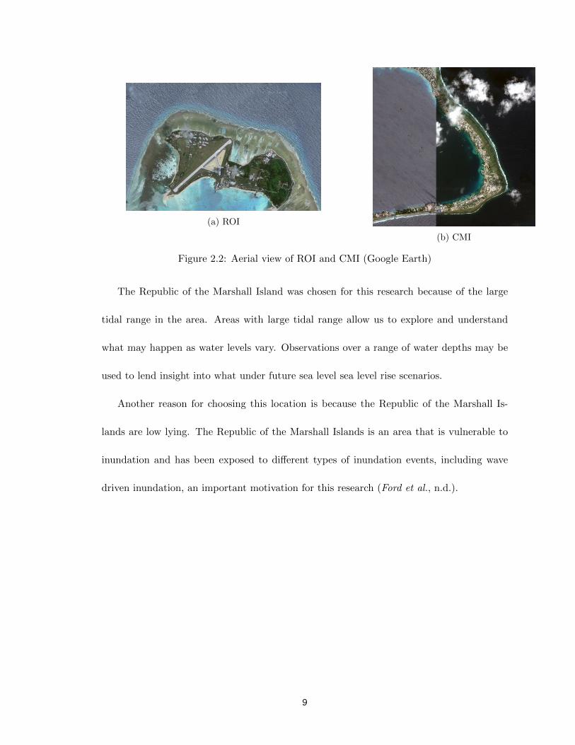
Figure 2.2: Aerial view of ROI and CMI (Google Earth)

The Republic of the Marshall Island was chosen for this research because of the large

tidal range in the area. Areas with large tidal range allow us to explore and understand

what may happen as water levels vary. Observations over a range of water depths may be

used to lend insight into what under future sea level sea level rise scenarios.

Another reason for choosing this location is because the Republic of the Marshall Is-

lands are low lying. The Republic of the Marshall Islands is an area that is vulnerable to

inundation and has been exposed to different types of inundation events, including wave

driven inundation, an important motivation for this research (Ford et al., n.d.).

9

CHAPTER 3: DATA

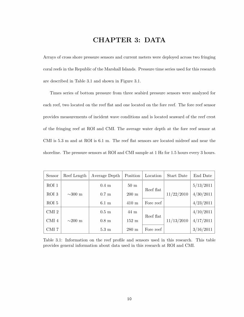
Arrays of cross shore pressure sensors and current meters were deployed across two fringing

coral reefs in the Republic of the Marshall Islands. Pressure time series used for this research

are described in Table 3.1 and shown in Figure 3.1.

Times series of bottom pressure from three seabird pressure sensors were analyzed for

each reef, two located on the reef flat and one located on the fore reef. The fore reef sensor

provides measurements of incident wave conditions and is located seaward of the reef crest

of the fringing reef at ROI and CMI. The average water depth at the fore reef sensor at

CMI is 5.3 m and at ROI is 6.1 m. The reef flat sensors are located midreef and near the

shoreline. The pressure sensors at ROI and CMI sample at 1 Hz for 1.5 hours every 3 hours.

Sensor Reef Length Average Depth Position Location Start Date End Date

ROI 1

∼300 m

0.4 m 50 mReef flat

11/22/2010

5/13/2011

ROI 3 0.7 m 200 m 4/30/2011

ROI 5 6.1 m 410 m Fore reef 4/23/2011

CMI 2

∼200 m

0.5 m 44 mReef flat

11/13/2010

4/10/2011

CMI 4 0.8 m 152 m 4/17/2011

CMI 7 5.3 m 280 m Fore reef 3/16/2011

Table 3.1: Information on the reef profile and sensors used in this research. This tableprovides general information about data used in this research at ROI and CMI.

10

0 50 100 150 200 250 300 350 400 450 500!15

!10

!5

0

5

h(m

)

ROI

1 3

5

Reef flat

Fore reef

0 50 100 150 200 250 300 350 400 450 500!15

!10

!5

0

5

h(m

)

R eef Length (Cross shore) [m]

CMI

2 4

7

Figure 3.1: Reef profile of (top) ROI and (bottom) CMI with the location of the bottompressure sensors. There are two sensors on the reef flat and one on the fore reef at eachcross shore location. For this research, the three seabird sensors at each reef are used.

11

CHAPTER 4: METHODS

4.1 WAVE CHARACTERISTICS AND PROPERTIES

A wave may be described by three main length scales; the wave length, the wave height

and the local water depth. Figure 4.1 shows a two dimensional general representation of a

monochomatic wave.

Figure 4.1: Wave properties. This figure shows general parameters in a simple one-dimensional wave. (Figure 1.1 from Dean and Dalrymple, 1991)

The wavelength, λ, is the horizontal distance between two crests of a wave, or two

troughs of a wave. The wave height, H, is the vertical distance between the crest and the

trough of a wave. Another measure of the vertical distance of a wave is the amplitude, a.

The amplitude is measured from the mean level of the wave to either the crest or the trough

of the wave and a = H/2 for a sinusoidal wave. The water depth, h, is measured from the

bottom of the ocean floor to the mean level of the wave.

12

The wave period is given by

T =2π

ω=

1

f, (4.1)

where f is the frequency and ω is the angular frequency.

The wave number is expressed as

k =2π

λ. (4.2)

Finally η is the free surface elevation of the wave which is a function of time and distance.

The dynamics of free surface elevation will be further discussed in Section 4.4.

4.2 DISPERSION RELATION

The dispersion relation for linear surface gravity waves of angular frequency ω, is defined

by the wave number and water depth, according to

ω =�

gk tanh(kh) (4.3)

where g is the gravitational acceleration.

This dispersion relation may be simplified depending on the water depth. The shallow-

ness of water is defined by the relative depth, related to the wavelength λ and the water

depth h. Shallow water waves have a large wave length with respect to water depth such

that kh � 1. For instance, when the water depth is 1 km and the wavelength, 20 km the

13

wave is considered to be in shallow water. Near the shoreline, the water depth is shallow

enough that the vertical dependence of the pressure is nearly uniform (Figure 4.2b). As the

water depth increases, the vertical dependance of the pressure decays with depth and the

water filters out the waves that are shorter in wavelength (Figure 4.2a).

The dispersion relation in shallow water reduces to

ω ≈�ghk . (4.4)

In the deep water limit, kh � 1 and the wavelength is much smaller than the water

depth. For deep water, the dispersion relation becomes

ω ≈�gk . (4.5)

The dispersion relationship Equation 4.3 describes the transition zone where deep water

waves propagates over an area with decreasing water depth and subsequently into shallow

water. The limits of the shallow water, deep water and for intermediate depths defined by

Dean and Dalrymple (1991) are shown in Table 4.1.

Shallow Water kh < π/10 h/λ < 1/20

Intermediate Depth π/10 < kh < π 1/20 < h/λ < 1/2

Deep Water kh > π h/λ > 1/2

Table 4.1: Definition of shallow, intermediate and deep water limits. (Dean and Dalrymple,1991).

14

(a) Deep Water

(b) Shallow Water

Figure 4.2: Difference of water particle orbits in deep and shallow water. In deep waters,the water particles beneath the waves are circular and decay with depth. For shallow water,the water particles are elliptically shaped. (Figure 7-4 from Pinet , 2009)

To account for intermediate depths, a function was made to solve Equation 4.3 for the

wave number k for given water depth, h, and the frequencies, f , of the wave. The function

is valid for all depths including the intermediate depths. This function is important to

account for the wavelength and water depth when calculating the free surface elevation.

4.3 DATA PROCESSING

For this research, the pressure time series are analyzed using Matlab® in an effort to

relate incident wave energy measured on the fore reef to the energy at the shoreline. The

largest observed shoreline response is due to low frequency motions on the reef flat.

15

The pressure time series are recorded in psi units. First, the raw pressure records are

converted to meters. The assumption is made that the atmospheric pressure is constant

since atmospheric pressure measurements were not taken concurrently.

Following the conversion, the linear trend and the mean are removed from the data by

using the Matlab® detrend function. This is to remove the tide which may be estimated

with a linear trend for the 1.5 hour records considered. The mean water level is removed

to focus on the dynamic pressure due to waves.

4.4 FREE SURFACE ELEVATION

For all sensors at ROI and CMI, the bottom pressure time series that have been detrended

are depth corrected to estimate the free surface elevation. As discussed in Section 4.2, the

waves at the shoreline are shallow water waves with pressure uniform in depth. Therefore,

the bottom pressure time series is a close estimate to the free surface elevation. On the

other hand, for waves in deeper water sites, the bottom pressure time series is no longer a

close estimate to the free surface elevation.

For all water depths, the free surface elevation is related to the bottom pressure, P

according to

η =P

ρgKp(−h), (4.6)

where ρ is the density of water and Kp is the pressure response factor,

16

Kp(−h) =1

cosh(kh). (4.7)

For shallow water (kh � 1)Kp → 1 and η = Pρg .

The function to calculate the dispersion relation, presented in Section 4.2, is used to

calculate the k, for a given water depth and frequency. Therefore, the pressure response

factor may be obtained as a function of frequency at a given sensor location. Since the

pressure response factor depends on the frequency, the high frequency range of the waves

will be amplified more. For the lower frequencies, the pressure response factor will have less

effect on the pressure data.

!0.3 !0.2 !0.1 0 0.1 0.2 0.30

0.2

0.4

0.6

0.8

1

Frequency (Hz)

(a) ROI 1

!0.3 !0.2 !0.1 0 0.1 0.2 0.30

1

2

3

4

5

6

7

8

9

10

11

Frequency (Hz)

(b) ROI 5

Figure 4.3: The pressure response factor for the bottom pressure time series in the frequencydomain for (a) ROI 1 and (b) ROI 5. At ROI 1, the water is nearly depth independent andthe pressure response factor is very close to a boxcar filter. At ROI 5, the higher frequenciescorrespond to waves in intermediate depths with amplitudes that decay with depth.

The pressure response factor is used to depth correct the bottom pressure time series

in the frequency domain. Figure 4.3a and 4.3b are the calculated pressure response factor

of ROI 1 and ROI 5 respectively. The bottom pressure series in the frequency domain

17

are multiplied by the pressure response factor to depth correct the data. As one can see in

Figure 4.3a, the band pass is nearly uniform as expected for nearly depth independent waves

of the reef flat. Also as shown in Figure 4.3b, it is clear that the pressure response factor is

much greater for high frequency waves as the deeper locations (Compare to Figure 4.3a).

ROI 1 and CMI 2 are in shallow water; therefore, the depth correction was assumed

to be small. However, by applying the depth correction to ROI 1 and CMI 2 it becomes

apparent that the depth correction creates slight structure. Therefore to be consistent, the

shallow water sensors are also treated with the depth correction factor.

Figure 4.4 shows the progression of the time series of free surface elevation at (a) ROI

and (b) CMI across the array. At both ROI and CMI, the figures clearly show there is an

overall decrease in the high frequency energy as the wave propagate shoreward. At ROI

and CMI, the low frequency component appears to increase shoreward.

03:00 03:05 03:10 03:15

!2

!1

0

1

2

03:00 03:05 03:10 03:15

!2

!1

0

1

2

Fre

e S

urf

ace

Ele

vatio

n (!

)

03:00 03:05 03:10 03:15

!2

!1

0

1

2

Time (min)

(a) ROI

09:00 09:05 09:10 09:15

!2

!1

0

1

2

09:00 09:05 09:10 09:15

!2

!1

0

1

2

09:00 09:05 09:10 09:15

!2

!1

0

1

2

Time (min)

(b) CMI

Figure 4.4: Fifteen minute free surface elevation time series and its cross shore transitionfrom off shore (top) to shore (bottom) of the free surface elevation at ROI and CMI. Thefore reef sensors at ROI and CMI show energetic high frequency motions. The sensors onthe reef flat show low frequency motions.

18

4.5 SIGNIFICANT WAVE HEIGHT

The measured time series are superpositions of waves of different amplitudes and frequencies.

Significant wave height is a statistical measure defined as the average of the highest 1/3

waves for a random wave field. For this research, the significant wave height is is calculated

by taking the standard deviation of the free surface elevation and multiplying by 4.

Figure 4.5 shows the significant wave height of ROI 1 and ROI 5 on a single figure.

Significant wave height of both ROI 1 and ROI 5 have several noticeable peaks. Being

relevant to inundation, these high peaks were identified for further analysis.

Dec Jan Feb Mar Apr0

0.5

1

1.5

2

2.5

3

Time (month)

Signifi

cantW

aveHeight(m

)

ROI 5ROI 1

Figure 4.5: Plot of significant wave height at ROI 1 (blue) and ROI 5 (black) against timeat ROI. The data with local water depth less than 10 cm are omitted from the analysis.High significant wave height shows energetic events and are the focus of this research.

19

4.6 BAND PASS FILTER

In order to look at the data in greater detail, the original 1.5 hour pressure time series

are reshaped into 900 second records. Similar to the initial data processing, the data is

converted into meters and the linear trend is removed. The linear trend here is removed

from each 900 second records. Moreover, the significant wave height is estimated for the

900 second record.

To further understand what is generating the high significant wave heights, the free

surface elevation is separated into two dynamically different frequency bands. First, the

pressure time series is Fourier transformed, and the data is then band pass filtered.

The two dynamically different frequency wave bands are the sea and swell frequency

band and the infragravity frequency band. For ROI and CMI, the sea and swell frequency

band 1/30 Hz < f < 0.35 Hz includes waves that are driven both by local and distant winds

and are energetic on the fore reef prior to wave breaking. The infragravity band 1/900 Hz <

f ≤ 1/30 Hz includes motions that are energetic on the reef flat. See Appendix A for more

information on the sensitivity of the significant wave height estimate due to the change in

band width for the sea and swell band and the infragravity band.

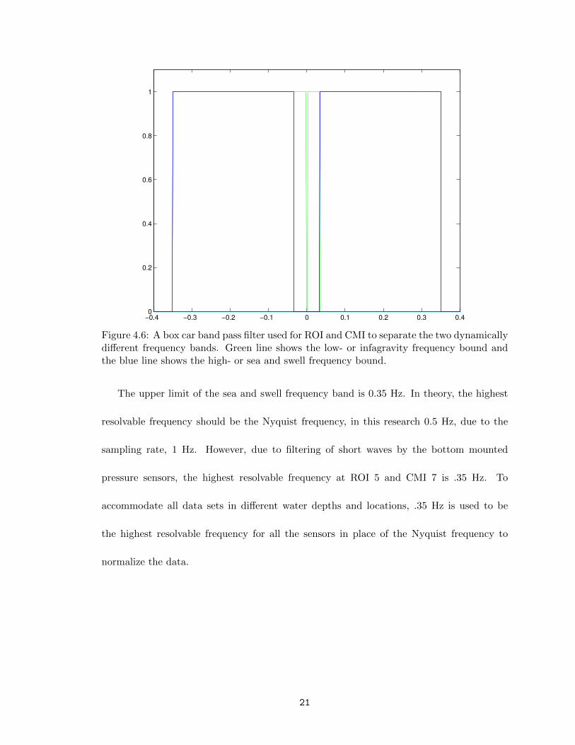
A boxcar band pass filter is created (Figure 4.6). After the array for the band pass

filter has been created, it is applied to the frequency domain pressure data to eliminate

the unwanted frequencies and separate the frequencies into the sea and swell band and the

infragravity band.

20

!0.4 !0.3 !0.2 !0.1 0 0.1 0.2 0.3 0.40

0.2

0.4

0.6

0.8

1

Figure 4.6: A box car band pass filter used for ROI and CMI to separate the two dynamicallydifferent frequency bands. Green line shows the low- or infagravity frequency bound andthe blue line shows the high- or sea and swell frequency bound.

The upper limit of the sea and swell frequency band is 0.35 Hz. In theory, the highest

resolvable frequency should be the Nyquist frequency, in this research 0.5 Hz, due to the

sampling rate, 1 Hz. However, due to filtering of short waves by the bottom mounted

pressure sensors, the highest resolvable frequency at ROI 5 and CMI 7 is .35 Hz. To

accommodate all data sets in different water depths and locations, .35 Hz is used to be

the highest resolvable frequency for all the sensors in place of the Nyquist frequency to

normalize the data.

21

03:00 03:05 03:10 03:15

!2

!1

0

1

2

Senso

r 5

03:00 03:05 03:10 03:15

!2

!1

0

1

2

Senso

r 3

03:00 03:05 03:10 03:15

!2

!1

0

1

2

Time (min)

Senso

r 1

(a) ROI: Sea and Swell (JAN 21, 2011)

03:00 03:05 03:10 03:15!0.4

!0.2

0

0.2

0.4

03:00 03:05 03:10 03:15!0.4

!0.2

0

0.2

0.4

03:00 03:05 03:10 03:15!0.4

!0.2

0

0.2

0.4

Time (min)

(b) ROI: Infragravity (JAN 21, 2011)

09:00 09:05 09:10 09:15!2

!1

0

1

2

Senso

r 7

09:00 09:05 09:10 09:15!2

!1

0

1

2

Time (min)

Senso

r 2

09:00 09:05 09:10 09:15!2

!1

0

1

2

Senso

r 4

(c) CMI: Sea and Swell (DEC 07,2010)

09:00 09:05 09:10 09:15!0.5

0

0.5

09:00 09:05 09:10 09:15!0.5

0

0.5

Time (min)

09:00 09:05 09:10 09:15!0.5

0

0.5

(d) CMI: Infragravity (DEC 07,2010)

Figure 4.7: Cross shore transformation of the free surface elevation at ROI in the (a)sea and swell frequency band and (b) infragravity frequency band and CMI (c) sea andswell frequency band and (d) infragravity frequency band. At both locations the fore reefsensor shows more energy in the sea and swell band, losing energy as the wave propagatesshoreward. The infragravity band shows more energy on the reef flat compared to the forereef.

4.7 AUTO SPECTRUM

To spectrally analyze the data, the free surface elevation estimated in Section 4.4 is Fourier

transformed into the frequency domain. One-sided spectra are calculated, where the nega-

tive frequencies are combined with the equivalent positive frequencies. Moreover, there is

22

no energy at f > 0.35 Hz, therefore the high frequency limit for this research, explained in

Section 4.5, is 0.35 Hz.

Without averaging the data, the spectral estimates have only two degrees of freedom,

thus the statistical reliability of the data is very low. Therefore, both band averaging and

ensemble averaging were tested on the spectral estimates to increase the degrees of freedom

of the data. For this research, band averaging of the data was found suitable to increase the

degrees of freedom to increase the reliability of the data. All of the data is averaged over 5

frequency bands, hence increasing the degrees of freedom to 10 to gain reliability and keep

sufficient frequency resolution.

4.8 LOWER FREQUENCY LIMIT

The record length of the data controls the low frequency limit. A longer record length will

result in a spectrum where the lower frequencies are better resolved. For ROI and CMI, the

lower frequencies were predominantly in the first bin after the mean, 1/T , when the record

is separated in 900 second record lengths. Therefore, analysis is done with the full record

length, which is 5400 seconds to increase the lower frequency resolution of the data.

23

CHAPTER 5: TIME DOMAIN ANALYSIS

The general characteristics of wave transformation over the reefs at ROI and CMI appear

similar. The majority of the energy in the free surface elevation is contained in the high

frequencies on the fore reef, whereas the free surface elevation on the reef flat near the

shoreline is dominated by low frequency energy. Finally, the free surface elevation at mid

reef is dominated by the low frequency energy; however, the high frequency energy is larger

at mid reef than near the shoreline.

5.1 CROSS SHORE TRANSFORMATION

The transformation of waves from the fore reef to the near shore is shown clearly in Fig-

ure 5.1. Figure 5.1a shows that the energy at the fore reef is dominantly in the sea and

swell frequencies. The amplitude of the sea and swell energy is much larger compared to

the infragravity energy, shown as the solid red line. This figure shows that the infragravity

energy is a small contribution to the wave energy at the fore reef.

On the other hand, the infragravity waves are dominant at the shoreline at ROI 1

(Figure 5.1b). In the 900 second wave burst, shown in Figure 5.1b, approximately two

oscillations of the infragravity wave are visually present, making the low frequency wave

period approximately 7.5 min. Moreover, the amplitudes of the infragravity waves are much

larger than those of the sea and swell waves. The sea and swell energy decreases greatly as

the wave propagates shoreward, and only provides a small contribution to the total energy

near the shoreline.

24

22:05 22:10 22:15!3

!2

!1

0

1

2

3

!(m

)

ROI: FEB 27, 2011

(a) ROI 5

22:05 22:10 22:15

!0.5

!0.4

!0.3

!0.2

!0.1

0

0.1

0.2

0.3

0.4

0.5

Time

!(m

)

ROI 1: FEB 27, 2011

(b) ROI 1

Figure 5.1: Free surface elevation at ROI in two dynamically different frequency bandswhere the red are the infragravity waves and the blue are the sea and swell waves at (a)ROI 5 and (b) ROI 1. This figure shows that ROI 5 is sea and swell wave dominant, whereasROI 1 is infragravity wave dominant.

5.2 SIGNIFICANT WAVE HEIGHT

At ROI, eight 1.5 hour time series of high significant wave height have been analyzed spec-

trally (Figure 5.2a). High significant wave height shows that the wave events are energetic.

Also, most of the high significant wave heights at ROI 5 are consistent with the peaks at

the shoreline sensor ROI 1. Five 1.5 hour time series of high significant wave height at CMI

are analyzed spectrally (Figure 5.3a) during the largest wave events.

25

Event Name Record No. Date

ROI

ROIe1 302 NOV 28, 2010

ROIe2 769 DEC 08, 2011

ROIe3 1147 DEC 16, 2010

ROIe4 2065 JAN 04, 2011

ROIe5 2635 JAN 16, 2011

ROIe6 2886 JAN 21, 2011

ROIe7 4697 FEB 27, 2011

ROIe8 5873 MAR 24, 2011

CMI

CMIe1 259 NOV 18, 2010

CMIe2 731 NOV 28, 2010

CMIe3 1875 DEC 22, 2010

CMIe4 3391 JAN 22, 2011

CMIe5 5116 FEB 27, 2011

Table 5.1: High energy events observed at ROI and CMI.

26

Dec

Jan

Feb

Mar

Ap

r0

0.51

1.52

2.53

Tim

e(m

onth

)

SignificantWaveHeight(m)

RO

I 5

RO

I 1

(a)

Dec

Jan

Feb

Mar

Apr

0

0.51

1.52

2.53

Tim

e(m

onth

s)

SignificantWaveHeight(m)

ROI:

Sea

andSwell

(b)

Dec

Jan

Feb

Mar

Apr

0

0.1

0.2

0.3

0.4

0.5

0.6

0.7

0.8

0.9

Tim

e(m

onth

s)

SignificantWaveHeight(m)

ROI:

Infragra

vity

(c)

Figure

5.2:

Significant

waveheigh

tat

ROIfor(a)allfrequen

cies

andfor(b)seaan

dsw

ellan

d(c)infrag

ravity

separately.

Thetotal

sign

ificant

waveheigh

tis

usedto

pickou

ten

ergeticevents

toan

alyzefurther.Theban

dpassedsign

ificant

waveheigh

tshow

sthat

the

seaan

dsw

ellen

ergy

isalwaysdom

inan

tat

ROI5,

andtheinfrag

ravity

energy

istypically

dom

inan

tat

ROI1.

27

Dec

Jan

Feb

Mar

0

0.51

1.52

2.5

Tim

e(m

onth

)

SignificantWaveHeight(m)

CM

I 7

CM

I 2

(a)

Dec

Jan

Feb

Mar

0

0.51

1.52

2.5

Tim

e(m

onth

s)

SignificantWaveHeight(m)

CMI:

Sea

andSwell

(b)

Dec

Jan

Feb

Mar

0

0.2

0.4

0.6

0.81

Tim

e(m

onth

s)

SignificantWaveHeight(m)

CMI:

Infragra

vity

(c)

Figure

5.3:

Significant

waveheigh

tat

CMIfor(a)allfrequen

cies

andfor(b)seaan

dsw

ellan

d(c)infrag

ravity

separately.

Thetotal

sign

ificant

waveheigh

tis

usedto

pickou

ten

ergeticevents

toan

alyzefurther.Theban

dpassedsign

ificant

waveheigh

tshow

sthat

the

seaan

dsw

ellen

ergy

isalwaysdom

inan

tat

CMI7,

andtheinfrag

ravity

energy

istypically

dom

inan

tat

CMI2.

28

Figure 5.2b, 5.2c, 5.3b and 5.3c shows how the sea and swell and the infragravity energy

transforms cross shore. These figures show the cross shore transformation over a larger time

period compared to Figure 5.1. The sea and swell plots show that there is a lot of energy

in the sea and swell frequency band at the fore reef before the waves break. On the other

hand, the infragravity bands at ROI and CMI shows that there more infragravity energy

on the reef flat compared to the fore reef. These plots show that the sea and swell energy

decreases shoreward, and the infragravity energy increases shoreward.

Further, the data are analyzed using scatter plots (Figure 5.5, 5.4 and 5.6). Figure 5.4a

is a scatter plot of 15 minute sea and swell significant wave height at ROI on the mid reef

versus shoreline, and colored with the local water level. This plot shows that the sea and

swell significant wave height is always lower at the shoreline (ROI 1) compared to mid reef

(ROI 3). Also the local water level color scale shows that there is more sea and swell energy

on the reef flat when there is more water on the reef flat. Therefore, the sea and swell

energy is predictable accordingly with the water level on the reef flat (Figure 5.5a). This

also is true at CMI. Figures 5.4b and 5.5b are equivalent to Figures 5.4a and 5.5a, but only

with the data collected at CMI. The two figures are very similar, and they both show that

the sea and swell energy decreases shoreward on the reef flat, and that sea and swell wave

height at the reef flat is an increasing function of water level.

On the other hand, the scatter plot of the infragravity energy at the shoreline versus

mid reef shows that there are times when the energy increased shoreward on the reef flat,

at both at ROI and CMI (Figure 5.6a and 5.6b). Both at ROI and CMI, the infragravity

energy increased shoreward on the reef flat when the local water level was high. The effect

29

of local water level on the infragravity energy is less evident than for the sea and swell,

however, higher water levels on the reef flat do allow more infragravity energy to reach the

shoreline. This does not mean that the infragravity waves are always large when the water

level is high. There are events that show high local water level but the infragravity energy

at ROI 1 and CMI 2 are lower than seen at ROI 3 and CMI 4.

For the infragravity energy, the scatter plot is also presented colored with the significant

wave height at the fore reef sensors (Figure 5.6). These plots show the relation of the energy

distribution on the reef flat depending on the energy seen on the fore reef. These plots show

that both at ROI and CMI, the infragravity energy content on the reef flat depends on the

energy at the fore reef sensor. Typically, more energy seen on the fore reef results in more

infragratity energy on the reef flat.

0 0.1 0.2 0.3 0.4 0.50

0.1

0.2

0.3

0.4

0.5

ROI 1

ROI3

ROI : SS Significant Wave Height (m)

LocalW

ate

rLevel(m

)

0.2

0.4

0.6

0.8

1

1.2

(a) ROI SS: Comparing reef flat sensors

0 0.1 0.2 0.3 0.4 0.5 0.6 0.70

0.1

0.2

0.3

0.4

0.5

0.6

CMI 2

CMI4

CMI : SS Significant Wave Height (m)

LocalW

ate

rLevel(m

)

0.2

0.4

0.6

0.8

1

1.2

(b) CMI SS: Comparing reef flat sensors

Figure 5.4: Scatter plots of sea and swell wave heights at the shoreline sensor versus themid reef sensor at (a) ROI and (b) CMI colored by local water level showing that sea andswell energy decays shoreward. Observations h < 0.1 m are omitted fro this analysis.

30

0 0.2 0.4 0.6 0.8 1 1.2 1.40

0.05

0.1

0.15

0.2

0.25

0.3

0.35

0.4

0.45

ROI : Significant Wave Height vs Water Leve l

Water Leve l (m)

ROI1:SS

(a) ROI SS: Comparing reef flat sensors

0 0.5 1 1.50

0.1

0.2

0.3

0.4

0.5

CMI : Significant Wave Height vs Water Leve l

Water Leve l (m)

CMI2:SS

(b) CMI SS: Comparing reef flat sensors

Figure 5.5: Scatter plots of shoreline sea and swell wave heights at (a) ROI and (b) CMIversus local water level. This figure shows clearly that the sea and swell waves, both at ROIand CMI are highly correlated with the local water depth.

31

0 0.2 0.4 0.6 0.8 10

0.1

0.2

0.3

0.4

0.5

0.6

0.7

0.8

ROI 1

ROI3

ROI : IG Significant Wave Height (m)

LocalW

ate

rLevel(m

)

0.2

0.4

0.6

0.8

1

1.2

(a) ROI IG: Local Water Level

0 0.2 0.4 0.6 0.8 1 1.20

0.1

0.2

0.3

0.4

0.5

0.6

0.7

0.8

CMI 2

CMI4

CMI : IG Significant Wave Height (m)

LocalW

ate

rLevel(m

)

0.2

0.4

0.6

0.8

1

1.2

(b) CMI IG: Local Water Level

0 0.2 0.4 0.6 0.8 10

0.1

0.2

0.3

0.4

0.5

0.6

0.7

0.8

ROI 1

ROI3

ROI : IG Significant Wave Height (m)

ROI5(S

S)

0.8

1

1.2

1.4

1.6

1.8

2

2.2

2.4

2.6

2.8

(c) ROI IG: Significant Wave Height ROI 5

0 0.2 0.4 0.6 0.8 1 1.20

0.1

0.2

0.3

0.4

0.5

0.6

0.7

0.8

CMI 2

CMI4

CMI : Significant Wave Height (m)

CMI7(S

S)

0.6

0.8

1

1.2

1.4

1.6

1.8

2

2.2

(d) CMI IG: Significant Wave Height CMI 7

Figure 5.6: Scatter plots of infragravity waves over the reef flat sensors at (a, c) ROI and(b, d) CMI. Figures show the relation with the (a, b) local water level or (c, d) the energyat the fore reef compared to the energy at the reef flat depending on the location of thesensors in the infragravity frequency band.

32

CHAPTER 6: WAVE DYNAMICS

6.1 LONG WAVE EQUATIONS: NORMAL MODES

On the reef flat, shallow water waves are also known as long waves. The free surface

elevation of a shallow water wave obeys the wave equation,

∂2η

∂t2= c

2 ∂2η

∂x2, (6.1)

where the speed of waves is c2 = gh, t is the time and x is the cross shore direction.

When the time dependance of η as expressed as a complex exponential,

η = η(x)eiωt , (6.2)

we find that the wave equation becomes an ordinary differential equation for the spatially

dependant amplitude of the free surface elevation

d2η

dx2+

ω2

ghη = 0 . (6.3)

Equation 6.3 is solved given the boundary conditions of dηdx = 0 at x = 0, and η = 0 at

x = L (Figure 6.1).

The general solution of Equation 6.3 is,

η = A cos(kx) +B sin(kx) . (6.4)

33

h

L

x = Lx = 0

Figure 6.1: Standing wave in an idealized reef where h is the water depth and L is the crossshore reef length.

At the antinode, where x = 0, dηdx = 0, we find that B = 0. At the node, where x = L,

η = 0, we find that η = A cos(kL) = 0; hence, knL = (2n+1)π2 .

The solution of Equation 6.3 and the boundary conditions is

η = A cos(2n+ 1)π

2Lx . (6.5)

The dispersion relation of long waves relate the frequency and wave number,

ωn =�ghkn (6.6a)

which may be rearranged to yield,

kn =ωn√gh

. (6.6b)

34

In Equation 6.5, kn is shown to be equal to (2n+1)π2L . From this and applying the

dispersion relation,

kn =(2n+ 1)π

2L=

ωn√gh

. (6.7)

or

ωn =�

gh(2n+ 1)π

2L(6.8)

The angular frequency is related to the period of oscillation,T , according to

ω =2π

T(6.9)

hence

Tn =4L

(2n+ 1)√gh

. (6.10a)

Letting n = 0, the period of the gravest mode, T0, is

T0 =4L√gh

. (6.10b)

35

CHAPTER 7: SPECTRAL ANALYSIS

By computing the auto spectra of different wave bursts during events with enhanced in-

fragravity energy on the reef flat, we find the observed frequency and spatial structure are

consistent with that of the gravest normal mode.

7.1 CROSS SHORE TRANSFORMATION

The cross shore transformation of the wave field shows energetic sea and swell at the fore

reef sensor that decays shoreward. Infragravity waves may be more energetic than the depth

limited sea and swell waves on the reef flat. Figure 7.1a is a log-log plot of the spectral

density of a 1.5 hour wave burst at ROI on February 27th, 2011. This figure shows this

cross shore transformation is consistent with the time domain analysis if Section 5.1. ROI

5 shows that the fore reef energy is largest in the sea and swell band. The energy in the

infragravity band at the fore reef sensor is significantly smaller than the energy in the sea

and swell band. The reef flat sensors, ROI 1 and 3, show a spectral peak frequency is at

3.15 × 10−3 Hz (T0 = 318 sec). There is more energy at the peak frequency at ROI 1, the

closest to the shoreline compared to ROI 3 on the mid reef consistent infragravity energy

increasing shoreward (Section 5.1 and Figure 5.1b).

The observations made at CMI are consistent with the observation at ROI. The spectral

transformation of Figure 7.1b is similar to Figure 7.1a. Again, at CMI 7, there is more energy

in the sea and swell band than in the infragravity band. Moreover, the peak frequencies at

CMI 4 and CMI 2 are 2.22×10−3 Hz (T0 = 450 sec) and the amplitude of this spectral peak

36

also is increasing shoreward. Again, this is consistent with observed increase in infragrativy

energy shoreward presented in Section 5.1 and Figure 5.1b.

37

10

!3

10

!2

10

!1

10

!4

10

!3

10

!2

10

!1

10

0

10

1

log(F

requen

cy)[H

z]

log(|X|2

!f)

ROI:

FEB

27,2011

95%

RO

I 1

RO

I 3

RO

I 5

(a)ROI

10

!3

10

!2

10

!1

10

!4

10

!3

10

!2

10

!1

10

0

10

1

log(F

requen

cy)[H

z]

log(|X|2

!f)

CMI:

FEB

27,2011

95%

CM

I 2

CM

I 4

CM

I 7

(b)CMI

Figure

7.1:

Spectral

den

sity

ofcrossshoretran

sformationof

waveen

ergy

at(a)ROIan

d(b)CMIwherethegreenlineis

thefore

reef

sensor,

theredlineis

themid-reefsensoran

dthebluelinethenearshoresensorplotted

onalog-logscale.

Thesefigu

resareban

daverag

edwith10

degrees

offreedom

.AtbothROIan

dCMIthereef

flat

sensors

havemoreen

ergy

intheinfrag

ravity

waveban

ds,where

thesensoron

theshorelinebeingmoreen

ergetic.

Ontheother

han

d,thefore

reef

sensors

havemoreen

ergy

intheseaan

dsw

ellwave

ban

d,an

dlittle

energy

intheinfrag

ravity

waveban

d.

38

7.2 EFFECT OF WATER LEVEL

In this section, we examine water level effects on the observed peak frequency of the waves

on the reef flat. Equation 6.10 shows that the water depth, h, on the reef flat affects the

peak frequency. At ROI, three 1.5 hour time series with average reef water levels (defined as

the average water level at the shoreline and the mid reef sensors) of 0.64 m, 0.93 m and 1.2

m are examined spectrally. Figure 7.2a is a plot of the spectral density of the free surface

time series for the different water levels. At 1.2 m water level, the observed peak frequency

is at 3.06×10−3 Hz (T0 = 327 sec). At 1.0 m, the observed peak frequency is 2.50×10−3 Hz

(T0 = 400 sec). Finally at 0.64 m, the peak frequency is at 1.76−3 Hz (T0 = 480 sec). The

observed decrease in peak frequency with water depth is consistent with Equation 6.10.

Similar to ROI, at CMI the observed spectral peak frequency increases as the water

level increases (Figure 7.2b). When the water level dependance is plotted at CMI, the peak

frequency at water level 1.2 m is 3.80× 10−3 Hz (T0 = 263 sec). At water level 1.0 m, the

peak frequency is at 3.61× 10−3 Hz (T0 = 277 sec). Finally at water level 0.91 m the peak

frequency is 2.31× 10−3 Hz (T0 = 432 sec), again consistent with Equation 6.10.

Table 7.1 also includes the theoretical peak period of the gravest mode calculated from

T0 = 4L/√gh. The theoretical peak period is similar to the observed peak period. Sources

of error in T0 are discussed in Appendix B. The dependance of theoretical period, on the

water level is consistent with the observations. Both at ROI and CMI, the peak period

is smaller when the water level on the reef flat is higher consistent with, T0 ∝ 1/√gh

(Equation 6.10).

39

Observed

Peak

Observed

Peak

TheoreticalPeak

RecordNo.

Date

Water

Level

(m)

Frequ

ency

(×10

−3Hz)

Period(sec)

Period(sec)

Con

stan

treef

lengthof

∼30

0m

(ROI)

2886

JAN

21,20

111.2

3.06

327

350

302

NOV

28,20

101.0

2.50

400

383

4697

FEB

27,20

110.64

1.76

568

480

Con

stan

treef

lengthof

∼20

0m

(CMI)

1875

DEC

22,20

101.2

3.80

263

219

731

NOV

28,20

101.0

3.61

277

260

259

NOV

18,20

100.91

2.31

432

279

Tab

le7.1:

Observed

peakfrequen

cyan

dperiodfrom

thespectral

analysis

described

inSection

7.2compared

withthetheoreticalpeak

period(E

quation6.10

).

40

12

34

56

7

x 1

0!

3

0

0.51

1.52

2.53

3.54

4.5

Frequen

cy(H

z)

|X|2

!f

ROI:

WaterLev

elDep

endance

1.2

m

1.0

m

0.6

4 m

(a)ROIwithdifferentwater

levels.Blueat

1.2m

,redat

0.93m

and

greenat

0.64

m.

12

34

56

7

x 1

0!

3

0

0.51

1.52

2.5

CMI:

WaterLev

elDep

endance

Frequen

cy(H

z)|X|2

!f

1.2

m

1.0

m

0.9

1 m

(b)CMIwithdifferentwater

levels.Blueat

1.2m

,redat

1.0m

and

greenat

0.90

m.

Figure

7.2:

Effectof

water

levelon

peakfrequen

cy.Auto

spectraof

thefree

surfaceelevationat

theshorelineat

(a)ROIan

d(b)CMI

forreef

flat

water

levelof

(blue)

∼1.2m

and(red

)∼1.0m

and(green

)∼0.64

mat

(a)ROIan

d∼0.91

mat

(b)CMI.Notehow

thepeak

frequen

cyat

higher

water

levels

arehigher

than

atlower

water

levels.

41

7.3 EFFECT OF REEF LENGTH

ROI and CMI are both fringing reefs but with different reef lengths. ROI has a reef length

of approximately 300 m and CMI has a reef length of approximately 200 m. The peak

frequency at ROI is lower compared to CMI for similar reef flat water levels. Figure 7.3a

shows a plot of the spectral density of ROI and CMI for a 1.5 hour free surface elevation

time series when the water level was approximately 1.0 m. The peak frequency at ROI is

2.50 × 10−3 Hz (T0 = 400 sec). Comparing the peak frequency to the peak frequency at

CMI, 3.61× 10−3 Hz (T0 = 260 sec), shows that the peak frequency is located at a higher

frequency compared to ROI.

At approximately 1.2 m water level (Figure 7.3b), we find that the observed peak fre-

quency at ROI 1 is 2.69× 10−3 Hz (T0 = 356 sec). At CMI 2, the observed peak frequency

is 3.80× 10−3 Hz (T0 = 219 sec). The larger observed peak period at ROI 1 versus CMI 2

is consistent with the reef length at ROI being larger than the reef length at CMI. These

findings show that the peak frequency is dependent on the geometry of the reef structure,

specifically the length of the reef. For the same reef flat water level, shorter reef have smaller

peak periods.

Moreover, the reef length ratio of the reef length at ROI to CMI (300 m/200 m) is 1.5,

and the observed peak periods also follow this ratio. In approximately 1.0 m depth, the

ratio is 400 sec/ 260 sec ∼1.5. In 1.2 m depth, the ratio is 356 sec/ 219 sec ∼1.6.

42

Table 7.2 also includes the theoretical peak period calculated from T0 = 4L/√gh. Again,

similar to Section 7.2 the theoretical peak period is similar to the observed peak period (See

Appendix B for errors).

43

Observed

Peak

Observed

Peak

TheoreticalPeak

RecordNo.

Date

ReefLength(m

)Frequ

ency

(×10

−3Hz)

Period(sec)

Period(sec)

Water

level∼

1.0m

302

NOV

28,2010

∼300(R

OI)

2.50

400

383

731

NOV

28,2010

∼200(C

MI)

3.61

277

260

Water

level∼

1.2m

2065

JAN

04,2011

∼300(R

OI)

2.69

372

356

1875

DEC

22,2010

∼200(C

MI)

3.80

263

219

Tab

le7.2:

Observed

peakfrequen

cyan

dperiodfrom

thespectral

analysis

described

inSection

7.3compared

withthetheoreticalpeak

period(E

quation6.10

).

44

12

34

56

7

x 1

0!

3

0

0.51

1.52

2.53

3.54

Frequen

cy(H

z)

|X|2

!f

WaterLev

el:!1.0m

CM

I

RO

I

(a)Effectof

chan

gein

reef

lengthat

∼1.0m

water

level

12

34

56

7

x 1

0!

3

0

0.51

1.52

2.5

Frequen

cy(H

z)|X|2

!f

WaterLev

el:!1.2m

CM

I

RO

I

(b)Effectof

chan

gein

reef

lengthat

∼1.2m

water

level

Figure

7.3:

Effectof

reef

lengthon

peakfrequen

cy.Auto

spectraof

thefree

surfaceelevationat

theshorelineat

(red

)CMIan

d(blue)

ROIforreef

flat

water

levelof

(a)∼1.0m

and(b)∼1.2m.Notehow

thepeakfrequen

cyat

ROIislower

than

atCMIforagivenwater

levelconsistentwiththelarger

reef

lengthat

ROI.

45

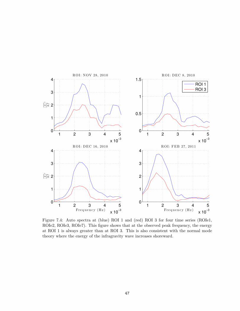
7.4 REEF FLAT TRANSFORMATION

By comparing different time series across the reef flat at ROI and CMI, we are able to

see how the infragravity energy transforms over the reef flat. At ROI 1 and ROI 3, when

the time series are spectrally analyzed, the spatial structure of the infragravity energy is

clear. Figure 7.4 shows the auto spectra for four 1.5 hour time series at ROI to compare the

amount of energy near the observed peak frequency at the shoreline (ROI 1) and mid reef

(ROI 3). The figures makes it clear that ROI 1 always has more energy near the observed

peak frequency compared to ROI 3. This is consistent with our results for Section 7.1 with

infragravity energy increasing shoreward and also from Equation 6.5 (n = 0) that describes

the spatial structure of the quarter-wavelength normal mode.

Figure 7.5 also shows four 1.5 hour time series spectrally analyzed, at CMI 2 and CMI

4. These figures show consistency with ROI, where the energy of the infragravity near the

observed peak frequency at CMI 2 is larger compared to CMI 4. This again is consistent

with what we expect to see in the quarter-wavelength normal mode (Equation 6.5, n = 0).

As the wave gets closer to the shoreline, the infragravity energy is larger than at the mid

reef sensors.

46

1 2 3 4 5

x 10!3

0

1

2

3

4

|X|2

!f

ROI : NOV 28, 2010

1 2 3 4 5

x 10!3

0

0.5

1

1.5

ROI : DEC 8, 2010

1 2 3 4 5

x 10!3

0

1

2

3

4

Freq uency (Hz )

|X|2

!f

ROI : DEC 16, 2010

1 2 3 4 5

x 10!3

0

1

2

3

4

Fre q uency (Hz )

ROI : FEB 27, 2011

ROI 1

ROI 3

Figure 7.4: Auto spectra at (blue) ROI 1 and (red) ROI 3 for four time series (ROIe1,ROIe2, ROIe3, ROIe7). This figure shows that at the observed peak frequency, the energyat ROI 1 is always greater than at ROI 3. This is also consistent with the normal modetheory where the energy of the infragravity wave increases shoreward.

47

2 4 6 8

x 10!3

0

0.5

1

1.5

2

2.5

|X|2

!f

CMI : NOV 28, 2010

2 4 6 8

x 10!3

0

0.5

1

1.5

2

CMI : DEC 22, 2010

2 4 6 8

x 10!3

0

0.5

1

1.5

Freq uency (Hz )

|X|2

!f

CMI : JAN 22, 2011

2 4 6 8

x 10!3

0

2

4

6

Freq uency (Hz )

CM I : FEB 27, 2011

CMI 2

CMI 4

Figure 7.5: Auto spectra at (blue) CMI 2 and (red) CMI 4 for four time series (CMIe2,CMIe3, CMIe4, CMIe5). This figure shows that at the observed peak frequency, the energyat CMI 2 is always greater than at CMI 4.

48

CHAPTER 8: DISCUSSION

The observations of infragravity wave events on the reef flat are consistent with the exci-

tation of a quarter-wavelength normal mode (Chapter 6). This normal mode infragravity

frequency and period depends on the water level and the reef length according to Equa-

tion 6.10. Section 7.2 and Table 7.1 show that the observed peak frequency depends on

the water level on the reef flat. Observations show that the peak frequency increases as the

water level increases over the reef flat.

Observations on two reefs of different lengths allowed us to test the theoretical depen-

dance of peak frequency on reef length. Section 7.3 and Table 7.2 shows the dependance

of the peak frequency due to the reef length. Comparing observations of peak period from

the ROI and CMI reefs, which have approximately 100 m difference in length, shows that

when the reef length is shorter, the peak frequency is larger, consistent with the theoretical

peak frequency Equation 6.10.

By comparing infragravity energy at the mid reef sensor and near shore sensor at ROI

and CMI, we found that the energy near the peak frequency increased shoreward consistent

with the excitation of a quarter-wavelength normal mode.

The modal excitation on the reef flat observed at ROI and CMI are consistent with the

studies of Nakaza et al. (1990) and Pequignet et al. (2009). The first modal period is given

by T0 = 4L/√gh. This equation shows that when the period is proportional to the reef

length, the period is also inversely proportional to the square root water level. These were

dependancies observed both at ROI and CMI.

49

For this research, we have omitted dissipation from Equation 6.1. Dissipation includes

the effects of friction over the reef flat. Dissipation may be important on reefs with longer

cross shore length, and also for shallow water depths over the reef flat, and is the topic of

further study.

An open question is how is the energy at the fore reef excites the normal modes on the

reef flat. Preliminarily, there have been studies that suggest that the forcing connected to

the infragravity energy is related to the envelope of the waves at the fore reef (Nakaza et al.,

1990; Nakaza and Hino, 1991; Gourlay , 1996; Pequignet et al., 2009; Nwogu and Demirbilek ,

2010; Van Dongeren et al., 2013). Nakaza et al. (1990) and Pequignet et al. (2009) related

the forcing of the infragravity waves on the reef flat to the wave envelope. The envelope of

the wave is energetic at frequencies similar to the normal modes (Figure 8.1).

A potential issue that may arise in the future is if the reef flat water level rises due

to sea level increases. It is well documented that large parts of the western pacific are

experiencing sea level rise (e.g., Merrifield and Maltrud , 2011; Perrette et al., 2013). This

research demonstrated that the increase in water level will decrease the period of a normal

mode. On the fringing reefs that Pequignet et al. (2009) and Pomeroy et al. (2012) studied,

they did not see modal excitation of infragravity waves over the reef flat during normal

conditions or at all. Sea level rise has the potential to increase the water level over these

shallow and long fringing reefs, which may facilitate the excitation of similar to what was

seen during Man-Yi at the Ipan reef (Pequignet et al., 2009).

Under elevated water levels, the potential for normal modes to be excited may increase.

The findings from this research suggests that the infragravity waves are and may become

50

22:05 22:10 22:15!2

!1.5

!1

!0.5

0

0.5

1

1.5

2

Time

!(m

)

ROI: FEB 27, 2011

ROI 5: Sea and SwellROI 5: EnvelopeROI 1: Infragravity

Figure 8.1: Free surface elevation of (blue) sea and swell component of the wave at ROI 5,the (black) envelope of the sea and swell component at ROI 5 and (red) the infragravitywave at ROI 1. This figure shows that the time scale of the envelope at ROI 5 and theinfragravity wave at ROI 1 are similar.

an increasingly more important component in wave driven inundation. Low lying areas

are already affected by sea level rise, just for the simple reason of the level of the land is

close to sea level. This research suggests that the risk of wave driven inundation also may

increase as sea level rise continues. Areas such as the Ipan reef under elevated water levels

may experience modal excitation on the reef as commonly as the Republic of the Marshall

Islands. These hypotheses are made under the assumption that the coral growth will be

limited and will not grow fast enough to maintain the current water level over the reef flat.

The forcing of these normal modes should be clarified to understand the infragravity waves

further in order to evaluate the risk and vulnerability of the low lying areas world wide.

51

APPENDIX A: BAND WIDTH

The sensitivity of the frequency limits of the band pass filter is considered here. The

appropriate frequency band of the infragravity and sea and swell depends on the spectral

content of the observations. This also means that the frequency limits of the bands are not

universal. Tests were conducted with different boundaries of the band pass filter. Table A.1

shows how the width of the band pass filter were arranged.

All (Hz) Infragravity (Hz) Sea and swell (Hz)

Original 1/900 < f < 0.35 1/900 < f ≤ 1/30 1/30 < f < 0.35

IG1/25 1/900 < f < 0.35 1/900 < f ≤ 1/25 1/25 < f < 0.35

IG1/20 1/900 < f < 0.35 1/900 < f ≤ 1/20 1/20 < f < 0.35

Table A.1: Data on the band width of the band pass filters used in this study.

The total band width has not been changed; however, the infragravity and sea and

swell band widths have been varied to determine their effects on significant wave height.

The assumption is that there will be more energy in the infragravity band, since more

frequencies have been added. Figure A.1 shows the difference in significant wave height due

to the change in the size of the band pass.

The figures makes it clear that the difference the width of the band pass filter is negligible

for this data set. There are some visible peaks seen in Figure A.1, however, the percentage

difference in the estimated significant wave height is negligible.

52

Nov

Dec

Jan

Feb

Mar

Apr

May

Jun

!101

All

Nov

Dec

Jan

Feb

Mar

Apr

May

Jun

0

0.0

2

0.0

4In

fragra

vity

Nov

Dec

Jan

Feb

Mar

Apr

May

Jun

!0.0

4

!0.0

20S

ea a

nd S

well

changed b

and (

b)

changed b

and (

a)

origin

al

(a)ROI1

Nov

Dec

Jan

Feb

Mar

Apr

May

!101

All

Nov

Dec

Jan

Feb

Mar

Apr

May

0

0.2

0.4

Infr

agra

vity

Nov

Dec

Jan

Feb

Mar

Apr

May

!0.1

!0.0

50S

ea a

nd S

well

chaned d

ata

(b)

changed d

ata

(a)

origin

al

(b)ROI5

Figure

A.1:Thedifferen

cesof

theban

dwidth

areexam

ined

withthesign

ificant

waveheigh

t.

53

APPENDIX B: PEAK PERIOD ERRORS

Theoretically, the peak period on the fringing reef is estimated from the quarter-wavelength

normal mode, formula T0 = 4L/√gh. When the theoretical period is calculated, the reef

length and the water level are the only two variables that affect the peak frequency. There-

fore the inaccuracy of the reef length will contribute to an error in estimating the theoretical

peak period.

Also, another error that may affect the theoretical peak period is the estimated water

level. For the time series analyzed here, the water level is gradually increasing or decreasing

due to the tidal effect. The water level is estimated by averaging the water depth during

the chosen time series at the two sensors on the reef flat. Therefore, when the time series

shows a tidally dependent water level, using a constant water level in the theoretical peak

period is questionable.

The theoretical period for the events selected for investigation shown in Figure 5.2a and

5.3a is compared with the observed peak period at ROI and CMI in Tables B.1 and B.2.

Due to the record length of the data, the frequency resolution at low frequency is limited.

Given the uncertainty of the water depth, the inaccuracy of the reef length and resolution

of the observed peak frequency, we find reasonable agreement between theoretical and peak

periods in Table B.1 and B.2.

54

Observed

Peak

Observed

Peak

TheoreticalPeak

RecordNo.

Date

Water

Level

(m)

Frequ

ency

(×10

−3Hz)

Period(sec)

Period(sec)

4697

FEB

27,20

110.64

1.76

568

480

1147

DEC

16,20

100.82

2.31

432

423

2635

JAN

16,20

110.84

3.06

372

417

769

DEC

08,20

110.93

2.50

400

397

302

NOV

28,20

101.0

2.50

400

383

2065

JAN

04,20

111.2

2.69

372

356

2886

JAN

21,20

111.2

3.06

327

350

Tab

leB.1:Observed

periodversustheoreticalperiodat

ROI.Bycomparingtheob

served

andtheoreticalpeakperiod,theperiodsshow

betterag

reem

entwhen

thewater

levels

arehigher.

55

Observed

Peak

Observed

Peak

TheoreticalPeak

RecordNo.

Date

Water

Level

(m)

Frequ

ency

(×10

−3Hz)

Period(sec)

Period(sec)

5116

MAR

08,20

110.84

2.31

432

279

259

NOV

27,20

100.91

2.31

432

268

731

DEC

07,20

101.0

3.61

277

260

1875

DEC

31,20

101.2

3.80

263

219

3391

JAN

31,20

111.2

3.06

327

227

Tab

leB.2:Observed

periodversustheoreticalperiodat

CMI.

56

REFERENCES

Dean, R. G., and R. A. Dalrymple (1991), Water wave mechanics for engineers andscientists, Advanced Series on Ocean Engineering, vol. 2, World Scientific Publishing CoInc.

Ford, M., J. M. Becker, and M. A. Merrifield (n.d.), Case studies of atoll islandinundation, Majuro Atoll, Republic of the Marshall Islands, Unpublished Draft.

Gourlay, M. R. (1996), Wave set-up on coral reefs. 2. Set-up on reefs with various profiles,Coastal Engineering, pp. 17–55.

Lugo-Fernandez, A., H. H. Roberts, and W. J. Wiseman, Jr (1998), Water level andcurrents of tidal and infragravity periods at Tague Reef, St. Croix (USVI), Coral Reefs.

Merrifield, M. A., and M. E. Maltrud (2011), Regional sea level trends due to a Pacifictrade wind intensification, Geophysical Research Letters, 38, doi:10.1029/2011GL049576.

Nakaza, E., and M. Hino (1991), Bore-like surf beat in a reef zone caused by wave groupsof incident short period waves, Fluid Dynamics Research, 7 (2), 89–100,doi:10.1016/0169-5983(91)90062-N.

Nakaza, E., S. Tsukayama, and M. Hino (1990), Bore-like surf beat on reef coasts, CoastalEngineering.

Nwogu, O., and Z. Demirbilek (2010), Infragravity wave motions and runup over shallowfringing reefs, Journal of Waterway, Port, Coastal, and Ocean Engineering.

Pequignet, A. C., J. M. Becker, M. A. Merrifield, and S. J. Boc (2011), The dissipation ofwind wave energy across a fringing reef at Ipan, Guam, Coral Reefs, 30 (S1), 71–82,doi:10.1007/s00338-011-0719-5.

Pequignet, A. C. N., J. M. Becker, M. A. Merrifield, and J. Aucan (2009), Forcing ofresonant modes on a fringing reef during tropical storm Man-Yi, Geophysical ResearchLetters, 36 (3), doi:10.1029/2008GL036259.

Perrette, M., F. Landerer, R. Riva, K. Frieler, and M. Meinshausen (2013), A scalingapproach to project regional sea level rise and its uncertainties, Earth SystemDynamics, 4 (1), 11–29, doi:10.5194/esd-4-11-2013.

Pinet, P. R. (2009), Essential invitation to oceanography, Burlington, MA : Jones &Bartlett Learning.

Pomeroy, A., R. Lowe, G. Symonds, C. Moore, and A. van Dongeren (2012), Thedynamics of infragravity wave transformation over a fringing reef, Journal ofGeophysical Research, 117 (C11), doi:10.1029/2012JC008310.

Spennemann, D. H. R. (1998), Non-traditional settlement patterns and typhoon hazard oncontemporary Majuro Atoll, Republic of the Marshall Islands.

Van Dongeren, A., R. Lowe, A. Pomeroy, D. M. Trang, D. Roelvink, G. Symonds, andR. Ranasinghe (2013), Numerical modeling of low-frequency wave dynamics over afringing coral reef, Coastal Engineering, 73, 178–190.

57

Vetter, O., J. M. Becker, M. A. Merrifield, A. C. Pequignet, J. Aucan, S. J. Boc, andC. E. Pollock (2010), Wave setup over a Pacific Island fringing reef, Journal ofGeophysical Research, 115 (C12), doi:10.1029/2010JC006455.

58